Embed Size (px)
Citation preview
Carbon dating is a method used to
determine the ages of archeological
artifacts up to 50,000 years old. For
example, archeologists are using
carbon dating to determine the ages
of the great pyramids of Egypt.
217
SELECTED APPLICATIONS
Exponential and logarithmic functions have many real-life applications. The applications listed below
represent a small sample of the applications in this chapter.
• Computer Virus,
Exercise 65, page 227
• Data Analysis: Meteorology,
Exercise 70, page 228
• Sound Intensity,
Exercise 90, page 238
• Galloping Speeds of Animals,
Exercise 85, page 244
• Average Heights,
Exercise 115, page 255
• Carbon Dating,
Exercise 41, page 266
• IQ Scores,
Exercise 47, page 266
• Forensics,
Exercise 63, page 268
• Compound Interest,
Exercise 135, page 273
3.1 Exponential Functions and Their Graphs
3.2 Logarithmic Functions and Their Graphs
3.3 Properties of Logarithms
3.4 Exponential and Logarithmic Equations
3.5 Exponential and Logarithmic Models
Exponential and
Logarithmic Functions 33©
Sy
lva
in G
ran
da
da
m/G
ett
y I
ma
ge
s
218 Chapter 3 Exponential and Logarithmic Functions
What you should learn
• Recognize and evaluate expo-
nential functions with base a.
• Graph exponential functions
and use the One-to-One
Property.
• Recognize, evaluate, and graph
exponential functions with
base e.
• Use exponential functions to
model and solve real-life
problems.
Why you should learn it
Exponential functions can be
used to model and solve real-life
problems. For instance, in
Exercise 70 on page 228, an
exponential function is used to
model the atmospheric pressure
at different altitudes.
Exponential Functions and Their Graphs
© Comstock Images/Alamy
3.1
Exponential Functions
So far, this text has dealt mainly with algebraic functions, which include poly-
nomial functions and rational functions. In this chapter, you will study two types
of nonalgebraic functions—exponential functions and logarithmic functions.
These functions are examples of transcendental functions.
The base is excluded because it yields This is a constant
function, not an exponential function.
You have evaluated for integer and rational values of For example, you
know that and However, to evaluate for any real number
you need to interpret forms with irrational exponents. For the purposes of this
text, it is sufficient to think of
(where )
as the number that has the successively closer approximations
Evaluating Exponential Functions
Use a calculator to evaluate each function at the indicated value of
Function Value
a.
b.
c.
Solution
Function Value Graphing Calculator Keystrokes Display
a. 2 3.1 0.1166291
b. 2 0.1133147
c. .6 3 2 0.4647580
Now try Exercise 1.
When evaluating exponential functions with a calculator, remember to
enclose fractional exponents in parentheses. Because the calculator follows the
order of operations, parentheses are crucial in order to obtain the correct result.
ENTERf s32d 5 s0.6d3y2
ENTERpf spd 5 22p
ENTERf s23.1d 5 223.1
x 532f sxd 5 0.6x
x 5 pf sxd 5 22x
x 5 23.1f sxd 5 2x
x.
a1.4, a1.41, a1.414, a1.4142, a1.41421, . . . .
!2 < 1.41421356a!2
x,4x41y2 5 2.43 5 64
x.ax
f sxd 5 1x
5 1.a 5 1
Definition of Exponential Function
The exponential function with base is denoted by
where and is any real number.xa > 0, a Þ 1,
f sxd 5 ax
af
x2c>
x2c>> dx 4
Example 1
The HM mathSpace® CD-ROM andEduspace® for this text contain additional resources related to the concepts discussed in this chapter.
Section 3.1 Exponential Functions and Their Graphs 219
x
g(x) = 4x
f(x) = 2x
y
−1−2−3−4 1 2 3 4−2
2
4
6
8
10
12
16
14
FIGURE 3.1
x
y
−1−2−3−4 1 2 3 4−2
4
6
8
10
12
14
16
G(x) = 4−x
F(x) = 2−x
FIGURE 3.2
Graphs of Exponential Functions
The graphs of all exponential functions have similar characteristics, as shown in
Examples 2, 3, and 5.
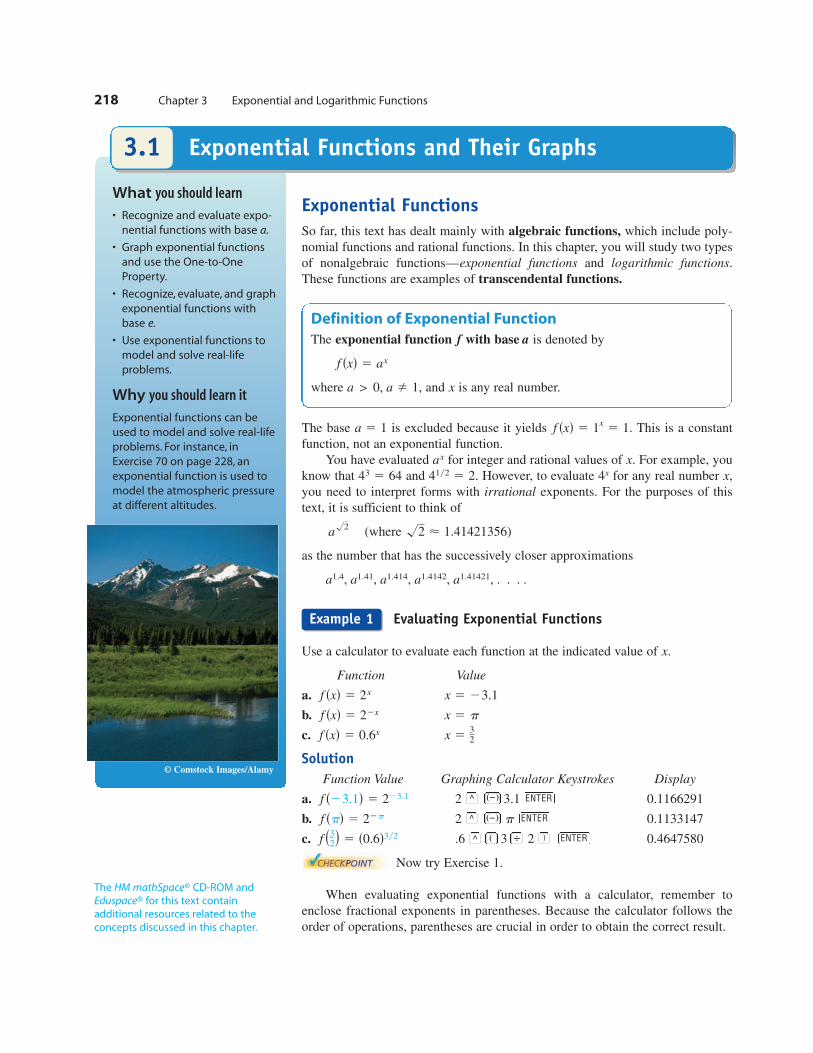
Graphs of y ax
In the same coordinate plane, sketch the graph of each function.
a. b.
Solution
The table below lists some values for each function, and Figure 3.1 shows the
graphs of the two functions. Note that both graphs are increasing. Moreover, the
graph of is increasing more rapidly than the graph of
Now try Exercise 11.
The table in Example 2 was evaluated by hand. You could, of course, use a
graphing utility to construct tables with even more values.
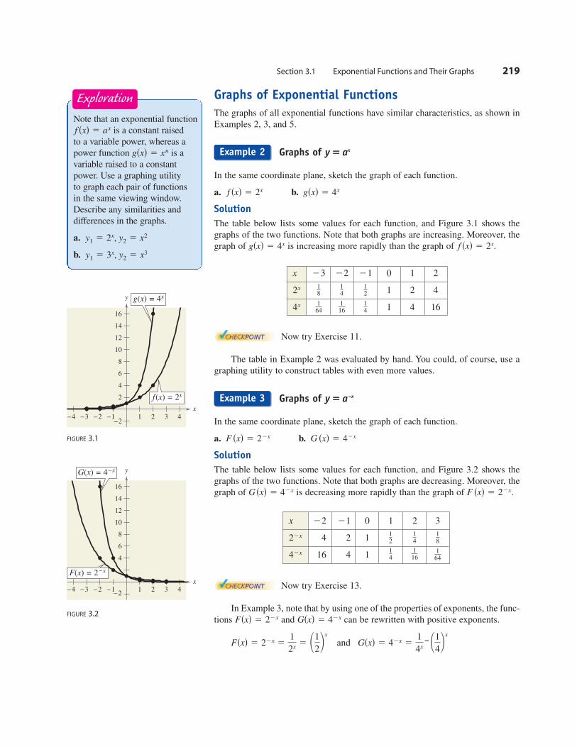
Graphs of y a–x
In the same coordinate plane, sketch the graph of each function.
a. b.
Solution
The table below lists some values for each function, and Figure 3.2 shows the
graphs of the two functions. Note that both graphs are decreasing. Moreover, the
graph of is decreasing more rapidly than the graph of
Now try Exercise 13.
In Example 3, note that by using one of the properties of exponents, the func-
tions and can be rewritten with positive exponents.
and Gsxd 5 42x 51
4x511
42x
Fsxd 5 22x 51
2x5 11
22x
Gsxd 5 42xFsxd 5 22x
F sxd 5 22x.Gsxd 5 42x
G sxd 5 42xF sxd 5 22x
5
f sxd 5 2x.gsxd 5 4x
gsxd 5 4xf sxd 5 2x
5
x 0 1 2
1 2 4
1 4 1614
116
1644x
12
14
182x
212223
x 0 1 2 3
4 2 1
16 4 1164
116
1442x
18
14
1222x
2122
Example 2
Example 3
Note that an exponential function
is a constant raised
to a variable power, whereas a
power function is a
variable raised to a constant
power. Use a graphing utility
to graph each pair of functions
in the same viewing window.
Describe any similarities and
differences in the graphs.
a.
b. y1 5 3x, y2 5 x3
y1 5 2x, y2 5 x2
gsxd 5 xn
f sxd 5 ax
Exploration
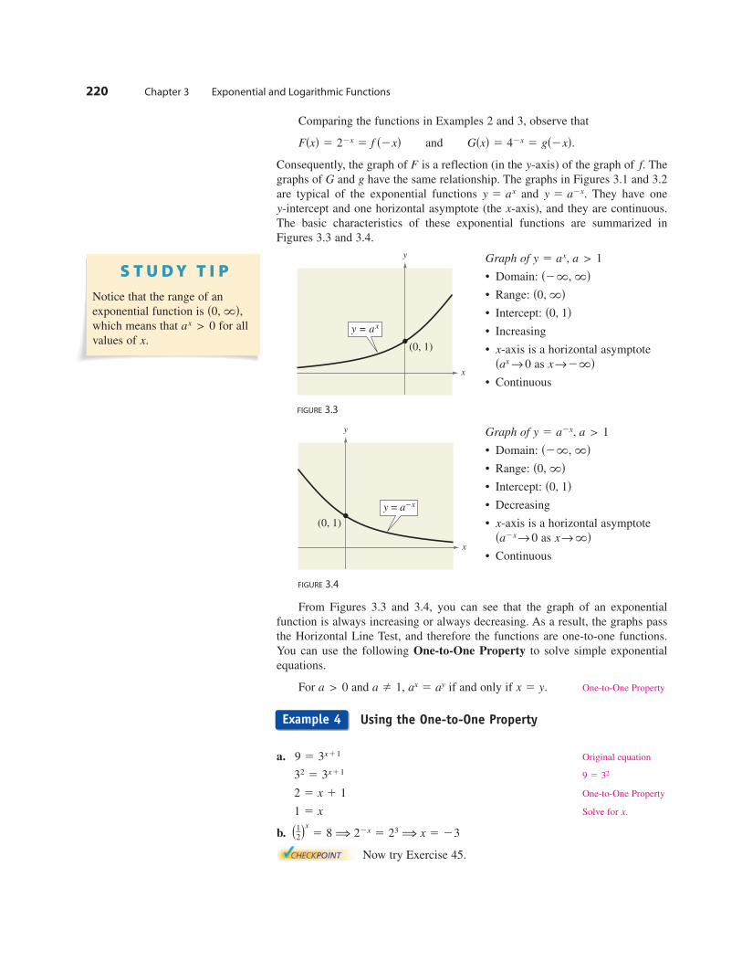
Comparing the functions in Examples 2 and 3, observe that
and
Consequently, the graph of is a reflection (in the -axis) of the graph of The
graphs of and have the same relationship. The graphs in Figures 3.1 and 3.2
are typical of the exponential functions and They have one
-intercept and one horizontal asymptote (the -axis), and they are continuous.
The basic characteristics of these exponential functions are summarized in
Figures 3.3 and 3.4.
Graph of
• Domain:
• Range:
• Intercept:
• Increasing
• -axis is a horizontal asymptote
as
• Continuous
Graph of
• Domain:
• Range:
• Intercept:
• Decreasing
• -axis is a horizontal asymptote
as
• Continuous
From Figures 3.3 and 3.4, you can see that the graph of an exponential
function is always increasing or always decreasing. As a result, the graphs pass
the Horizontal Line Test, and therefore the functions are one-to-one functions.
You can use the following One-to-One Property to solve simple exponential
equations.
For and if and only if One-to-One Property
Using the One-to-One Property
a. Original equation
One-to-One Property
Solve for
b.
Now try Exercise 45.
s12d
x
5 8 ⇒ 22x 5 23 ⇒ x 5 23
x. 1 5 x
2 5 x 1 1
9 5 32 32 5 3x11
9 5 3x11
x 5 y.ax 5 aya Þ 1,a > 0
x→`dsa2x→ 0
x
s0, 1d
s0, `d
s2`, `d
y 5 a2x, a > 1
x→2`dsax→ 0
x
s0, 1d
s0, `d
s2`, `d
y 5 ax, a > 1
xy
y 5 a2x.y 5 ax
gG
f.yF
Gsxd 5 42x 5 gs2xd.Fsxd 5 22x 5 f s2xd
220 Chapter 3 Exponential and Logarithmic Functions
Notice that the range of an
exponential function is
which means that for all
values of x.
ax> 0
s0, `d,
x
y = ax
(0, 1)
y
FIGURE 3.3
x
(0, 1)
y
y = a−x
FIGURE 3.4
Example 4
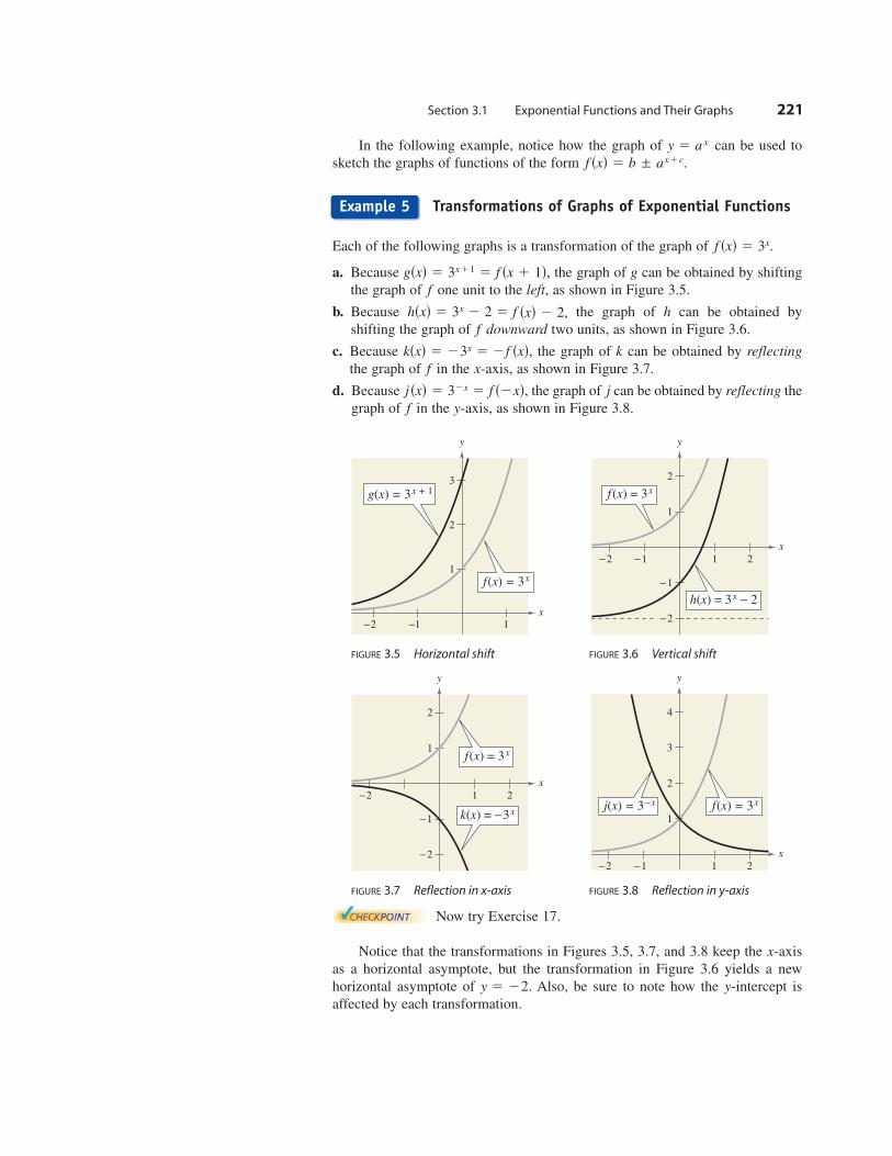
In the following example, notice how the graph of can be used to
sketch the graphs of functions of the form
Transformations of Graphs of Exponential Functions
Each of the following graphs is a transformation of the graph of
a. Because the graph of can be obtained by shifting
the graph of one unit to the left, as shown in Figure 3.5.
b. Because the graph of can be obtained by
shifting the graph of downward two units, as shown in Figure 3.6.
c. Because the graph of can be obtained by reflecting
the graph of in the -axis, as shown in Figure 3.7.
d. Because the graph of can be obtained by reflecting the
graph of in the -axis, as shown in Figure 3.8.
FIGURE 3.5 Horizontal shift FIGURE 3.6 Vertical shift
FIGURE 3.7 Reflection in x-axis FIGURE 3.8 Reflection in y-axis
Now try Exercise 17.
Notice that the transformations in Figures 3.5, 3.7, and 3.8 keep the -axis
as a horizontal asymptote, but the transformation in Figure 3.6 yields a new
horizontal asymptote of Also, be sure to note how the -intercept is
affected by each transformation.
yy 5 22.
x
x
f(x) = 3xj(x) = 3−x
21−1−2
1
2
3
4
y
x
f(x) = 3x
k(x) = −3x
21−2
1
−1
−2
2
y
x
21−1−2
1
−1
2
y
f (x) = 3x
h(x) = 3x − 2
−2x
−1−2 1
1
2
3
g(x) = 3x + 1
f(x) = 3x
y
yf
jjsxd 5 32x 5 f s2xd,xf
kksxd 5 23x 5 2f sxd,f
hhsxd 5 3x 2 2 5 f sxd 2 2,
f
ggsxd 5 3x11 5 f sx 1 1d,
f sxd 5 3x.
f sxd 5 b ± ax1c.
y 5 a x
Section 3.1 Exponential Functions and Their Graphs 221
Example 5
222 Chapter 3 Exponential and Logarithmic Functions
x
1−1−2
2
3
(0, 1)
(1, e)
(−1, e−1)
(−2, e−2)
f(x) = ex
y
FIGURE 3.9
x
4−4 3−3 2−2 1−1
f(x) = 2e0.24x
1
3
4
5
6
7
8
y
FIGURE 3.10
x
−4 −2 −1−3 4321
g(x) = e−0.58x
1
3
2
4
5
6
7
8
12
y
FIGURE 3.11
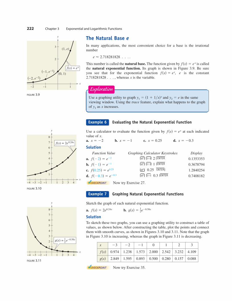
The Natural Base e
In many applications, the most convenient choice for a base is the irrational
number
This number is called the natural base. The function given by is called
the natural exponential function. Its graph is shown in Figure 3.9. Be sure
you see that for the exponential function is the constant
whereas is the variable.
Evaluating the Natural Exponential Function
Use a calculator to evaluate the function given by at each indicated
value of
a. b. c. d.
Solution
Function Value Graphing Calculator Keystrokes Display
a. 2 0.1353353
b. 1 0.3678794
c. 0.25 1.2840254
d. 0.3 0.7408182
Now try Exercise 27.
Graphing Natural Exponential Functions
Sketch the graph of each natural exponential function.
a. b.
Solution
To sketch these two graphs, you can use a graphing utility to construct a table of
values, as shown below. After constructing the table, plot the points and connect
them with smooth curves, as shown in Figures 3.10 and 3.11. Note that the graph
in Figure 3.10 is increasing, whereas the graph in Figure 3.11 is decreasing.
Now try Exercise 35.
gsxd 512e20.58xf sxd 5 2e0.24x
ENTERf s20.3d 5 e20.3
ENTERf s0.25d 5 e0.25
ENTERf s21d 5 e21
ENTERf s22d 5 e22
x 5 20.3x 5 0.25x 5 21x 5 22
x.
f sxd 5 ex
x2.718281828 . . . ,
ef sxd 5 ex,
f sxd 5 e x
e < 2.718281828 . . . .
ex
ex
ex
ex
x2c
x2c
x2c
x 0 1 2 3
0.974 1.238 1.573 2.000 2.542 3.232 4.109
2.849 1.595 0.893 0.500 0.280 0.157 0.088gsxd
f sxd
212223
Use a graphing utility to graph and in the same
viewing window. Using the trace feature, explain what happens to the graph
of as increases.xy1
y2 5 ey1 5 s1 1 1yxdx
Exploration
Example 6
Example 7
Applications
One of the most familiar examples of exponential growth is that of an investment
earning continuously compounded interest. Using exponential functions, you can
develop a formula for interest compounded times per year and show how it
leads to continuous compounding.
Suppose a principal is invested at an annual interest rate compounded
once a year. If the interest is added to the principal at the end of the year, the new
balance is
This pattern of multiplying the previous principal by is then repeated each
successive year, as shown below.
Year Balance After Each Compounding
0
1
2
3
To accommodate more frequent (quarterly, monthly, or daily) compounding
of interest, let be the number of compoundings per year and let be the num-
ber of years. Then the rate per compounding is and the account balance after
years is
Amount (balance) with compoundings per year
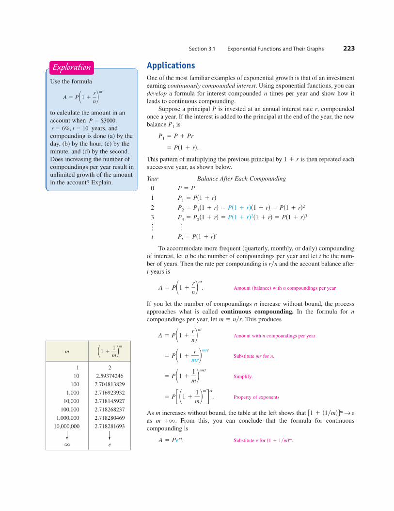
If you let the number of compoundings increase without bound, the process
approaches what is called continuous compounding. In the formula for
compoundings per year, let This produces
Amount with compoundings per year
Substitute for
Simplify.
Property of exponents
As increases without bound, the table at the left shows that
as From this, you can conclude that the formula for continuous
compounding is
Substitute for s1 1 1ymdm.eA 5 Pert.
m →`.
f1 1 s1ymdgm → em
5 P311 11
m2m
4rt
.
5 P11 11
m2mrt
n.mr 5 P11 1r
mr2mrt
n A 5 P11 1r
n2nt
m 5 nyr.
n
n
nA 5 P11 1r
n2nt
.
t
ryn
tn
Pt 5 Ps1 1 rdtt
. .
.. . .
P3 5 P2s1 1 rd 5 Ps1 1 rd2s1 1 rd 5 Ps1 1 rd3
P2 5 P1s1 1 rd 5 Ps1 1 rds1 1 rd 5 Ps1 1 rd2
P1 5 Ps1 1 rdP 5 P
1 1 r
5 Ps1 1 rd.
P1 5 P 1 Pr
P1
r,P
n
Section 3.1 Exponential Functions and Their Graphs 223
1 2
10 2.59374246
100 2.704813829
1,000 2.716923932
10,000 2.718145927
100,000 2.718268237
1,000,000 2.718280469
10,000,000 2.718281693
e`
11 11
m2m
m
Use the formula
to calculate the amount in an
account when
years, and
compounding is done (a) by the
day, (b) by the hour, (c) by the
minute, and (d) by the second.
Does increasing the number of
compoundings per year result in
unlimited growth of the amount
in the account? Explain.
r 5 6%, t 5 10
P 5 $3000,
A 5 P11 1r
n2nt
Exploration
Compound Interest
A total of $12,000 is invested at an annual interest rate of 9%. Find the balance
after 5 years if it is compounded
a. quarterly.
b. monthly.
c. continuously.
Solution
a. For quarterly compounding, you have So, in 5 years at 9%, the
balance is
Formula for compound interest
Substitute for and
Use a calculator.
b. For monthly compounding, you have So, in 5 years at 9%, the
balance is
Formula for compound interest
Substitute for and
Use a calculator.
c. For continuous compounding, the balance is
Formula for continuous compounding
Substitute for and
Use a calculator.
Now try Exercise 53.
In Example 8, note that continuous compounding yields more than quarterly
or monthly compounding. This is typical of the two types of compounding. That
is, for a given principal, interest rate, and time, continuous compounding will
always yield a larger balance than compounding times a year.n
< $18,819.75.
t.r,P, 5 12,000e0.09(5)
A 5 Pert
< $18,788.17.
t.n,r,P, 5 12,00011 10.09
12 212(5)
A 5 P11 1r
n2nt
n 5 12.
< $18,726.11.
t.n,r,P, 5 12,00011 10.09
4 24(5)
A 5 P11 1r
n2nt
n 5 4.
224 Chapter 3 Exponential and Logarithmic Functions
Formulas for Compound Interest
After years, the balance in an account with principal and annual
interest rate (in decimal form) is given by the following formulas.
1. For compoundings per year:
2. For continuous compounding: A 5 Pe rt
A 5 P11 1r
n2nt
n
r
PAt
Example 8
Be sure you see that the annual
interest rate must be written in
decimal form. For instance, 6%
should be written as 0.06.
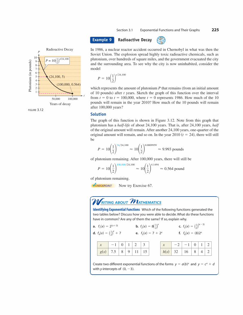
Radioactive Decay
In 1986, a nuclear reactor accident occurred in Chernobyl in what was then the
Soviet Union. The explosion spread highly toxic radioactive chemicals, such as
plutonium, over hundreds of square miles, and the government evacuated the city
and the surrounding area. To see why the city is now uninhabited, consider the
model
which represents the amount of plutonium that remains (from an initial amount
of 10 pounds) after years. Sketch the graph of this function over the interval
from to where represents 1986. How much of the 10
pounds will remain in the year 2010? How much of the 10 pounds will remain
after 100,000 years?
Solution
The graph of this function is shown in Figure 3.12. Note from this graph that
plutonium has a half-life of about 24,100 years. That is, after 24,100 years, half
of the original amount will remain. After another 24,100 years, one-quarter of the
original amount will remain, and so on. In the year 2010 there will still
be
of plutonium remaining. After 100,000 years, there will still be
of plutonium remaining.
Now try Exercise 67.
< 0.564 pound< 1011
224.1494
P 5 1011
22100,000y24,100
< 9.993 pounds< 1011
220.0009959
P 5 1011
2224y24,100
st 5 24d,
t 5 0t 5 100,000,t 5 0
t
P
P 5 1011
22ty24,100
Section 3.1 Exponential Functions and Their Graphs 225P
luto
niu
m (
in p
ounds)
Years of decay
t
PRadioactive Decay
1
2P = 10
t/24,100( (
50,000 100,000
1
2
3
4
5
6
7
8
9
10
(24,100, 5)
(100,000, 0.564)
FIGURE 3.12
W RITING ABOUT MATHEMATICS
Identifying Exponential Functions Which of the following functions generated the
two tables below? Discuss how you were able to decide. What do these functions
have in common? Are any of them the same? If so, explain why.
a. b. c.
d. e. f.
Create two different exponential functions of the forms and
with y-intercepts of s0, 23d.
y 5 cx 1 dy 5 asbdx
f6sxd 5 s8d2xf5sxd 5 7 1 2xf4sxd 5 s 1
2dx1 7
f3sxd 5 s 1
2d(x23)f2sxd 5 8s
1
2dxf1sxd 5 2(x13)
Example 9
x 0 1 2 3
7.5 8 9 11 15gsxd
21 x 0 1 2
32 16 8 4 2hsxd
2122
In Exercises 1– 6, evaluate the function at the indicated
value of Round your result to three decimal places.
Function Value
1.
2.
3.
4.
5.
6.
In Exercises 7–10, match the exponential function with its
graph. [The graphs are labeled (a), (b), (c), and (d).]
(a) (b)
(c) (d)
7. 8.
9. 10.
In Exercises 11–16, use a graphing utility to construct a
table of values for the function. Then sketch the graph of
the function.
11. 12.
13. 14.
15. 16.
In Exercises 17–22, use the graph of to describe the
transformation that yields the graph of
17.
18.
19.
20.
21.
22.
In Exercises 23–26, use a graphing utility to graph the
exponential function.
23. 24.
25. 26.
In Exercises 27–32, evaluate the function at the indicated
value of Round your result to three decimal places.
Function Value
27.
28.
29.
30.
31.
32. x 5 20f sxd 5 250e0.05x
x 5 6f sxd 5 5000e0.06x
x 5 240f sxd 5 1.5exy2
x 5 10f sxd 5 2e25x
x 5 3.2f sxd 5 ex
x 534hsxd 5 e2x
x.
y 5 4x11 2 2y 5 3x22 1 1
y 5 32|x|y 5 22x 2
gsxd 5 20.3x 1 5f sxd 5 0.3x,
gsxd 5 2s72d2x16
f sxd 5 s72dx
,
gsxd 5 102 x13f sxd 5 10x,
gsxd 5 5 2 2xf sxd 5 22x,
gsxd 5 4x 1 1f sxd 5 4x,
gsxd 5 3x24f sxd 5 3x,
g.
f
f sxd 5 4x23 1 3f sxd 5 2x21
f sxd 5 6xf sxd 5 62x
f sxd 5 s12d2x
f sxd 5 s12dx
f sxd 5 2x22f sxd 5 22x
f sxd 5 2x 1 1f sxd 5 2x
4
2
6
4
−2
−2 2−4
x
y
4
6
4−2
−2 2−4
x
y
4
2
6
4
−2
−2 2 6x
y
4
6
42
−2
−2−4
x
y
x 5 24f sxd 5 200s1.2d12x
x 5 21.5gsxd 5 5000s2xdx 5
310f sxd 5 s2
3d5x
x 5 2pf sxd 5 5x
x 532f sxd 5 2.3x
x 5 5.6f sxd 5 3.4x
x.
226 Chapter 3 Exponential and Logarithmic Functions
Exercises 3.1 The HM mathSpace® CD-ROM and Eduspace® for this text contain step-by-step solutions to all odd-numbered exercises. They also provide Tutorial Exercises for additional help.
VOCABULARY CHECK: Fill in the blanks.
1. Polynomials and rational functions are examples of ________ functions.
2. Exponential and logarithmic functions are examples of nonalgebraic functions, also called ________ functions.
3. The exponential function given by is called the ________ ________ function, and the base
is called the ________ base.
4. To find the amount in an account after years with principal and an annual interest rate compounded
times per year, you can use the formula ________.
5. To find the amount in an account after years with principal and an annual interest rate compounded
continuously, you can use the formula ________.
PREREQUISITE SKILLS REVIEW: Practice and review algebra skills needed for this section at www.Eduspace.com.
rPtA
n
rPtA
ef sxd 5 ex
Section 3.1 Exponential Functions and Their Graphs 227
In Exercises 33–38, use a graphing utility to construct a
table of values for the function. Then sketch the graph of
the function.
33. 34.
35. 36.
37. 38.
In Exercises 39– 44, use a graphing utility to graph the
exponential function.
39. 40.
41. 42.
43. 44.
In Exercise 45–52, use the One-to-One Property to solve the
equation for
45. 46.
47. 48.
49. 50.
51. 52.
Compound Interest In Exercises 53–56, complete the
table to determine the balance for dollars invested at
rate for years and compounded times per year.
53. years
54. years
55. years
56. years
Compound Interest In Exercises 57– 60, complete the
table to determine the balance for $12,000 invested at
rate for years, compounded continuously.
57. 58.
59. 60.
61. Trust Fund On the day of a child’s birth, a deposit of
$25,000 is made in a trust fund that pays 8.75% interest,
compounded continuously. Determine the balance in this
account on the child’s 25th birthday.
62. Trust Fund A deposit of $5000 is made in a trust fund
that pays 7.5% interest, compounded continuously. It is
specified that the balance will be given to the college from
which the donor graduated after the money has earned
interest for 50 years. How much will the college receive?
63. Inflation If the annual rate of inflation averages 4% over
the next 10 years, the approximate costs of goods or
services during any year in that decade will be modeled by
where is the time in years and is the
present cost. The price of an oil change for your car is
presently $23.95. Estimate the price 10 years from now.
64. Demand The demand equation for a product is given by
where is the price and is the number of units.
(a) Use a graphing utility to graph the demand function for
and
(b) Find the price for a demand of units.
(c) Use the graph in part (a) to approximate the greatest
price that will still yield a demand of at least 600 units.
65. Computer Virus The number of computers infected by
a computer virus increases according to the model
where is the time in hours. Find (a)
(b) and (c)
66. Population The population (in millions) of Russia
from 1996 to 2004 can be approximated by the model
where represents the year, with
corresponding to 1996. (Source: Census Bureau,
International Data Base)
(a) According to the model, is the population of Russia
increasing or decreasing? Explain.
(b) Find the population of Russia in 1998 and 2000.
(c) Use the model to predict the population of Russia in
2010.
67. Radioactive Decay Let represent a mass of radioactive
radium (in grams), whose half-life is 1599 years.
The quantity of radium present after years is
(a) Determine the initial quantity (when ).
(b) Determine the quantity present after 1000 years.
(c) Use a graphing utility to graph the function over the
interval to
68. Radioactive Decay Let represent a mass of carbon
(in grams), whose half-life is 5715 years. The quan-
tity of carbon 14 present after years is
(a) Determine the initial quantity (when ).
(b) Determine the quantity present after 2000 years.
(c) Sketch the graph of this function over the interval
to t 5 10,000.
t 5 0
t 5 0
Q 5 10s12dty5715
.t
14 s14CdQ
t 5 5000.t 5 0
t 5 0
Q 5 25s12dty1599
.
t
s226RadQ
t 5 6tP 5 152.26e20.0039t,
P
Vs2d.Vs1.5d,Vs1d,tVstd 5 100e4.6052t,
V
x 5 500p
p > 0.x > 0
xp
p 5 500011 24
4 1 e20.002x2
PtCstd 5 Ps1.04dt,
C
r 5 3.5%r 5 6.5%
r 5 6%r 5 4%
tr
A
P 5 $1000, r 5 6%, t 5 40
P 5 $2500, r 5 3%, t 5 20
P 5 $1000, r 5 4%, t 5 10
P 5 $2500, r 5 2.5%, t 5 10
ntr
PA
ex216 5 e5xex2
23 5 e2x
e2x21 5 e4e3x12 5 e3
11
52x11
5 1252x22 51
32
2x23 5 163x11 5 27
x.
hsxd 5 e x22gsxd 5 1 1 e2x
sstd 5 3e20.2tsstd 5 2e0.12t
y 5 1.085xy 5 1.0825x
f sxd 5 2 1 e x25f sxd 5 2ex22 1 4
f sxd 5 2e20.5xf sxd 5 3ex14
f sxd 5 e2xf sxd 5 ex
n 1 2 4 12 365 Continuous
A
t 10 20 30 40 50
A
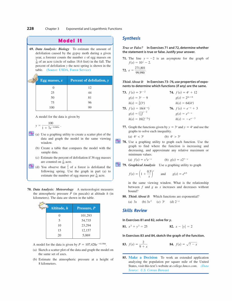
70. Data Analysis: Meteorology A meteorologist measures
the atmospheric pressure (in pascals) at altitude (in
kilometers). The data are shown in the table.
A model for the data is given by
(a) Sketch a scatter plot of the data and graph the model on
the same set of axes.
(b) Estimate the atmospheric pressure at a height of
8 kilometers.
Synthesis
True or False? In Exercises 71 and 72, determine whether
the statement is true or false. Justify your answer.
71. The line is an asymptote for the graph of
72.
Think About It In Exercises 73–76, use properties of expo-
nents to determine which functions (if any) are the same.
73. 74.
75. 76.
77. Graph the functions given by and and use the
graphs to solve each inequality.
(a) (b)
78. Use a graphing utility to graph each function. Use the
graph to find where the function is increasing and
decreasing, and approximate any relative maximum or
minimum values.
(a) (b)
79. Graphical Analysis Use a graphing utility to graph
and
in the same viewing window. What is the relationship
between and as increases and decreases without
bound?
80. Think About It Which functions are exponential?
(a) (b) (c) (d)
Skills Review
In Exercises 81 and 82, solve for .
81. 82.
In Exercises 83 and 84, sketch the graph of the function.
83. 84.
85. Make a Decision To work an extended application
analyzing the population per square mile of the United
States, visit this text’s website at college.hmco.com. (Data
Source: U.S. Census Bureau)
f sxd 5 !7 2 xf sxd 52
9 1 x
x 2 |y| 5 2x 2 1 y 2 5 25
y
22x3x3x 23x
xgf
gsxd 5 e0.5f sxd 5 11 10.5
x 2x
gsxd 5 x232xf sxd 5 x 2e2x
4x> 3x4x
< 3x
y 5 4xy 5 3x
hsxd 5 2ex23hsxd 5 16s222xdgsxd 5 e32xgsxd 5 s 1
4dx22
f sxd 5 e2x 1 3f sxd 5 16s42xdhsxd 5 64s4xdhsxd 5
19s3xd
gsxd 5 22x16gsxd 5 3x 2 9
f sxd 5 4x 1 12f sxd 5 3x22
e 5271,801
99,990.
f sxd 5 10x 2 2.
y 5 22
P 5 107,428e 20.150h.
hP
228 Chapter 3 Exponential and Logarithmic Functions
69. Data Analysis: Biology To estimate the amount of
defoliation caused by the gypsy moth during a given
year, a forester counts the number of egg masses on
of an acre (circle of radius 18.6 feet) in the fall. The
percent of defoliation the next spring is shown in the
table. (Source: USDA, Forest Service)
A model for the data is given by
(a) Use a graphing utility to create a scatter plot of the
data and graph the model in the same viewing
window.
(b) Create a table that compares the model with the
sample data.
(c) Estimate the percent of defoliation if 36 egg masses
are counted on acre.
(d) You observe that of a forest is defoliated the
following spring. Use the graph in part (a) to
estimate the number of egg masses per acre.140
23
140
y 5100
1 1 7e20.069x .
y
140
x
Model It
Egg masses, x Percent of defoliation, y
0 12
25 44
50 81
75 96
100 99
Altitude, h Pressure, P
0 101,293
5 54,735
10 23,294
15 12,157
20 5,069

Section 3.2 Logarithmic Functions and Their Graphs 229
Logarithmic Functions
In Section 1.9, you studied the concept of an inverse function. There, you learned
that if a function is one-to-one—that is, if the function has the property that no
horizontal line intersects the graph of the function more than once—the function
must have an inverse function. By looking back at the graphs of the exponential
functions introduced in Section 3.1, you will see that every function of the form
passes the Horizontal Line Test and therefore must have an inverse
function. This inverse function is called the logarithmic function with base a.
The equations
and
are equivalent. The first equation is in logarithmic form and the second is in
exponential form. For example, the logarithmic equation can be
rewritten in exponential form as The exponential equation can
be rewritten in logarithmic form as
When evaluating logarithms, remember that logarithm is an exponent.
This means that is the exponent to which must be raised to obtain For
instance, because 2 must be raised to the third power to get 8.
Evaluating Logarithms
Use the definition of logarithmic function to evaluate each logarithm at the indi-
cated value of
a. b.
c. d.
Solution
a. because
b. because
c. because
d. because
Now try Exercise 17.
1022 51
102 51
100.f s 1100d 5 log10
1100 5 22
41y2 5 !4 5 2.f s2d 5 log4 2 512
30 5 1.f s1d 5 log3 1 5 0
25 5 32.f s32d 5 log2 32 5 5
x 51
100f sxd 5 log10 x,x 5 2f sxd 5 log4 x,
x 5 1f sxd 5 log3 x,x 5 32f sxd 5 log2 x,
x.
log2 8 5 3
x.aloga x
a
log5 125 5 3.
53 5 1259 5 32.
2 5 log3 9
x 5 a yy 5 loga x
f sxd 5 ax
What you should learn
• Recognize and evaluate loga-
rithmic functions with base a.
• Graph logarithmic functions.
• Recognize, evaluate, and graph
natural logarithmic functions.
• Use logarithmic functions to
model and solve real-life
problems.
Why you should learn it
Logarithmic functions are often
used to model scientific obser-
vations. For instance, in Exercise
89 on page 238, a logarithmic
function is used to model
human memory.
Logarithmic Functions and Their Graphs
© Ariel Skelley/Corbis
3.2
Remember that a logarithm is
an exponent. So, to evaluate the
logarithmic expression
you need to ask the question,
“To what power must be
raised to obtain ”x?
a
loga x,
Definition of Logarithmic Function with Base a
For and
if and only if
The function given by
Read as “log base of ”
is called the logarithmic function with base a.
x.af sxd 5 loga x
x 5 ay.y 5 loga x
a Þ 1,a > 0,x > 0,
Example 1
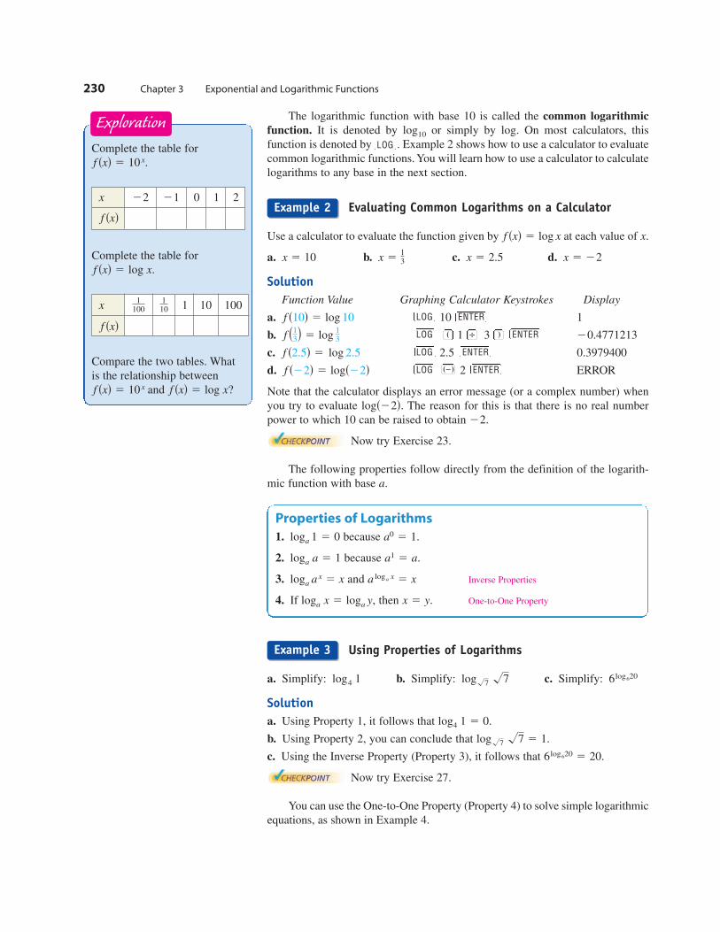
230 Chapter 3 Exponential and Logarithmic Functions
Complete the table for
Complete the table for
Compare the two tables. What
is the relationship between
and f sxd 5 log x?f sxd 5 10 x
f sxd 5 log x.
f sxd 5 10 x.
Exploration
x 0 1 2
f sxd
2122
x 1 10 100
f sxd
110
1100
The logarithmic function with base 10 is called the common logarithmic
function. It is denoted by or simply by log. On most calculators, this
function is denoted by . Example 2 shows how to use a calculator to evaluate
common logarithmic functions. You will learn how to use a calculator to calculate
logarithms to any base in the next section.
Evaluating Common Logarithms on a Calculator
Use a calculator to evaluate the function given by at each value of
a. b. c. d.
Solution
Function Value Graphing Calculator Keystrokes Display
a. 10 1
b. 1 3
c. 2.5 0.3979400
d. 2 ERROR
Note that the calculator displays an error message (or a complex number) when
you try to evaluate The reason for this is that there is no real number
power to which 10 can be raised to obtain
Now try Exercise 23.
The following properties follow directly from the definition of the logarith-
mic function with base
Using Properties of Logarithms
a. Simplify: b. Simplify: c. Simplify:
Solution
a. Using Property 1, it follows that
b. Using Property 2, you can conclude that
c. Using the Inverse Property (Property 3), it follows that
Now try Exercise 27.
You can use the One-to-One Property (Property 4) to solve simple logarithmic
equations, as shown in Example 4.
6log620 5 20.
log!7 !7 5 1.
log4 1 5 0.
6log620log!7 !7log4 1
a.
22.
logs22d.
ENTERLOGf s22d 5 logs22dENTERLOGf s2.5d 5 log 2.5
20.4771213ENTERLOGf s13d 5 log
13
ENTERLOGf s10d 5 log 10
x 5 22x 5 2.5x 513x 5 10
x.f sxd 5 log x
LOG
log10
Properties of Logarithms
1. because
2. because
3. and Inverse Properties
4. If then One-to-One Propertyx 5 y.loga x 5 loga y,
a loga x 5 xloga ax 5 x
a1 5 a.loga a 5 1
a0 5 1.loga 1 5 0
x2c
cx 4
Example 2
Example 3
Section 3.2 Logarithmic Functions and Their Graphs 231
x
−2 2 4 6 8 10
−2
2
4
6
8
10
g(x) = log2 x
f(x) = 2xy
y = x
FIGURE 3.13
x
1 2 3 4 5 6 7 8 9 10−1
−2
1
2
3
4
5
y
f(x) = log x
Vertical asymptote: x = 0
FIGURE 3.14
Using the One-to-One Property
a. Original equation
One-to-One Property
b.
c.
Now try Exercise 79.
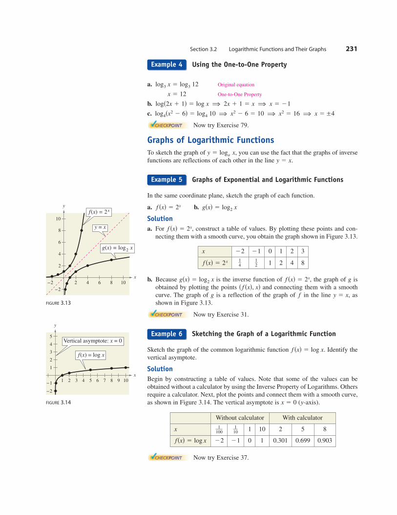
Graphs of Logarithmic Functions
To sketch the graph of you can use the fact that the graphs of inverse
functions are reflections of each other in the line
Graphs of Exponential and Logarithmic Functions
In the same coordinate plane, sketch the graph of each function.
a. b.
Solution
a. For construct a table of values. By plotting these points and con-
necting them with a smooth curve, you obtain the graph shown in Figure 3.13.
b. Because is the inverse function of the graph of is
obtained by plotting the points and connecting them with a smooth
curve. The graph of is a reflection of the graph of in the line as
shown in Figure 3.13.
Now try Exercise 31.
Sketching the Graph of a Logarithmic Function
Sketch the graph of the common logarithmic function Identify the
vertical asymptote.
Solution
Begin by constructing a table of values. Note that some of the values can be
obtained without a calculator by using the Inverse Property of Logarithms. Others
require a calculator. Next, plot the points and connect them with a smooth curve,
as shown in Figure 3.14. The vertical asymptote is ( -axis).
Now try Exercise 37.
yx 5 0
f sxd 5 log x.
y 5 x,fg
s f sxd, xdgf sxd 5 2x,gsxd 5 log2 x
f sxd 5 2x,
gsxd 5 log2 xf sxd 5 2x
y 5 x.
y 5 loga x,
log4sx2 2 6d 5 log4 10 ⇒ x2 2 6 5 10 ⇒ x2 5 16 ⇒ x 5 ±4
logs2x 1 1d 5 log x ⇒ 2x 1 1 5 x ⇒ x 5 21
x 5 12
log3 x 5 log3 12
Without calculator With calculator
x 1 10 2 5 8
0 1 0.301 0.699 0.9032122fsxd 5 log x
110
1100
x 0 1 2 3
1 2 4 812
14f sxd 5 2x
2122
Example 4
Example 5
Example 6
232 Chapter 3 Exponential and Logarithmic Functions
You can use your understanding
of transformations to identify
vertical asymptotes of logarith-
mic functions. For instance,
in Example 7(a) the graph of
shifts the graph
of one unit to the right. So,
the vertical asymptote of is
one unit to the right of
the vertical asymptote of the
graph of f sxd.
x 5 1,
gsxdf sxd
gsxd 5 f sx 2 1d
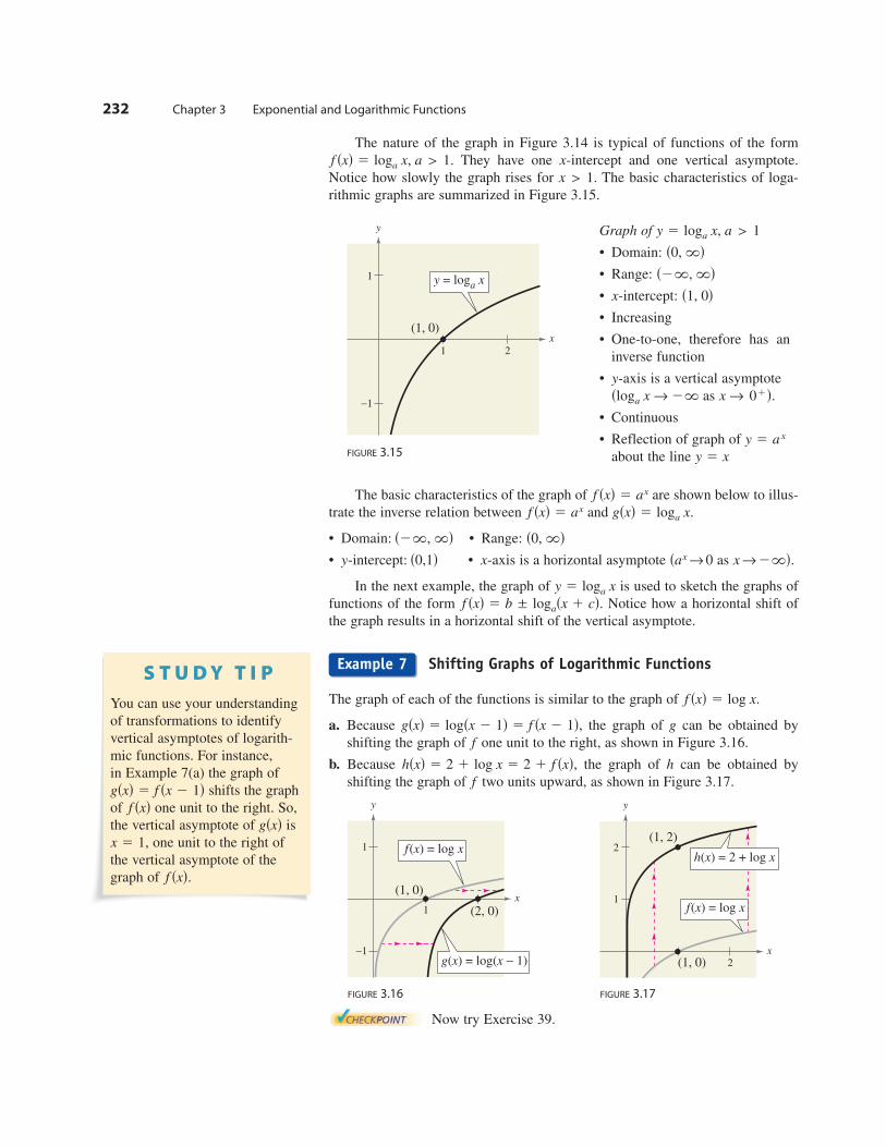
The nature of the graph in Figure 3.14 is typical of functions of the form
They have one -intercept and one vertical asymptote.
Notice how slowly the graph rises for The basic characteristics of loga-
rithmic graphs are summarized in Figure 3.15.
The basic characteristics of the graph of are shown below to illus-
trate the inverse relation between and
• Domain: • Range:
• -intercept: • -axis is a horizontal asymptote as
In the next example, the graph of is used to sketch the graphs of
functions of the form Notice how a horizontal shift of
the graph results in a horizontal shift of the vertical asymptote.
Shifting Graphs of Logarithmic Functions
The graph of each of the functions is similar to the graph of
a. Because the graph of can be obtained by
shifting the graph of one unit to the right, as shown in Figure 3.16.
b. Because the graph of can be obtained by
shifting the graph of two units upward, as shown in Figure 3.17.
FIGURE 3.16 FIGURE 3.17
Now try Exercise 39.
x
(1, 0)
(1, 2)
1
2
2
y
h(x) = 2 + log x
f(x) = log xx
(1, 0)
(2, 0)1
1
−1
y
f(x) = log x
g(x) = log(x − 1)
f
hhsxd 5 2 1 log x 5 2 1 f sxd,f
ggsxd 5 logsx 2 1d 5 f sx 2 1d,
f sxd 5 log x.
f sxd 5 b ± logasx 1 cd.y 5 loga x
x → 2`d.sax → 0xs0,1dy
s0, `ds2`, `d
gsxd 5 loga x.f sxd 5 ax
f sxd 5 ax
x > 1.
xf sxd 5 loga x, a > 1.
x
1
−1
1 2
(1, 0)
y
y = loga x
FIGURE 3.15
Graph of
• Domain:
• Range:
• -intercept:
• Increasing
• One-to-one, therefore has an
inverse function
• -axis is a vertical asymptote
as
• Continuous
• Reflection of graph of
about the line y 5 x
y 5 a x
01d.x →sloga x → 2`y
s1, 0dx
s2`, `ds0, `d
y 5 loga x, a > 1
Example 7
Section 3.2 Logarithmic Functions and Their Graphs 233
x
32−1−2
3
2
−1
−2
(e, 1)
( )(1, 0)
1e( )−1,
g(x) = f −1(x) = ln x
(1, e)
(0, 1)
y = x
y
, −11e
f(x) = ex
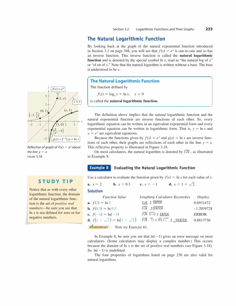
Reflection of graph of about
the line
FIGURE 3.18
y 5 x
f sxd 5 ex
Notice that as with every other
logarithmic function, the domain
of the natural logarithmic func-
tion is the set of positive real
numbers—be sure you see that
ln is not defined for zero or for
negative numbers.
x
The Natural Logarithmic Function
By looking back at the graph of the natural exponential function introduced
in Section 3.1 on page 388, you will see that is one-to-one and so has
an inverse function. This inverse function is called the natural logarithmic
function and is denoted by the special symbol ln read as “the natural log of ”
or “el en of ” Note that the natural logarithm is written without a base. The base
is understood to be
The definition above implies that the natural logarithmic function and the
natural exponential function are inverse functions of each other. So, every
logarithmic equation can be written in an equivalent exponential form and every
exponential equation can be written in logarithmic form. That is, and
are equivalent equations.
Because the functions given by and are inverse func-
tions of each other, their graphs are reflections of each other in the line
This reflective property is illustrated in Figure 3.18.
On most calculators, the natural logarithm is denoted by , as illustrated
in Example 8.
Evaluating the Natural Logarithmic Function
Use a calculator to evaluate the function given by for each value of
a. b. c. d.
Solution
Function Value Graphing Calculator Keystrokes Display
a. 2 0.6931472
b. .3 –1.2039728
c. 1 ERROR
d. 1 2 0.8813736
Now try Exercise 61.
In Example 8, be sure you see that gives an error message on most
calculators. (Some calculators may display a complex number.) This occurs
because the domain of ln is the set of positive real numbers (see Figure 3.18).
So, is undefined.
The four properties of logarithms listed on page 230 are also valid for
natural logarithms.
lns21dx
lns21d
ENTERLNf s1 1 !2 d 5 lns1 1 !2 dENTERLNf s21d 5 lns21d
ENTERLNf s0.3d 5 ln 0.3
ENTERLNf s2d 5 ln 2
x 5 1 1 !2x 5 21x 5 0.3x 5 2
x.f sxd 5 ln x
LN
y 5 x.
gsxd 5 ln xf sxd 5 e x
x 5 e y
y 5 ln x
e.
x.
xx,
f sxd 5 ex
The Natural Logarithmic Function
The function defined by
is called the natural logarithmic function.
f sxd 5 loge x 5 ln x, x > 0
x2c
dx ! 1
Example 8
234 Chapter 3 Exponential and Logarithmic Functions
Using Properties of Natural Logarithms
Use the properties of natural logarithms to simplify each expression.
a. b. c. d.
Solution
a. Inverse Property b. Inverse Property
c. Property 1 d. Property 2
Now try Exercise 65.
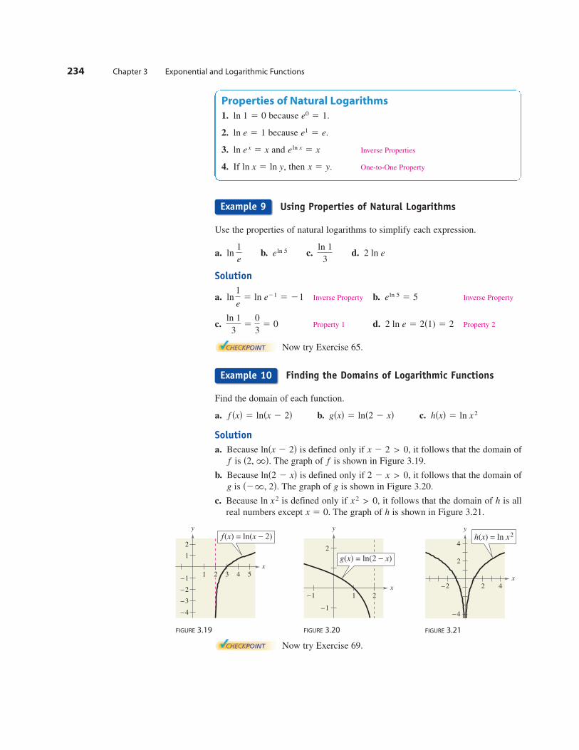
Finding the Domains of Logarithmic Functions
Find the domain of each function.
a. b. c.
Solution
a. Because is defined only if it follows that the domain of
is The graph of is shown in Figure 3.19.
b. Because is defined only if it follows that the domain of
is The graph of is shown in Figure 3.20.
c. Because is defined only if it follows that the domain of is all
real numbers except The graph of is shown in Figure 3.21.
Now try Exercise 69.
hx 5 0.
hx2> 0,ln x2
gs2`, 2d.g
2 2 x > 0,lns2 2 xdfs2, `d.f
x 2 2 > 0,lnsx 2 2d
hsxd 5 ln x2gsxd 5 lns2 2 xdf sxd 5 lnsx 2 2d
2 ln e 5 2s1) 5 2ln 1
35
0
35 0
eln 5 5 5ln 1
e5 ln e21 5 21
2 ln eln 1
3eln 5ln
1
e
x
2
−1g(x) = ln(2 − x)
y
−1
−1
1 2
FIGURE 3.20
x
y
f(x) = ln(x − 2)
1
1
−1
−2
−3
−4
2
3 4 52
FIGURE 3.19
x
y
h(x) = ln x2
−2 2 4
2
−4
4
FIGURE 3.21
Properties of Natural Logarithms
1. because
2. because
3. and Inverse Properties
4. If then One-to-One Propertyx 5 y.ln x 5 ln y,
eln x 5 xln e x 5 x
e1 5 e.ln e 5 1
e0 5 1.ln 1 5 0
Example 9
Example 10
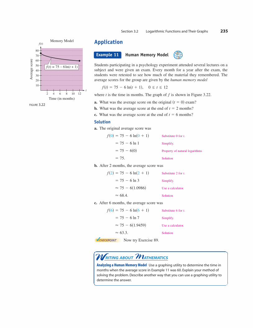
Application
Human Memory Model
Students participating in a psychology experiment attended several lectures on a
subject and were given an exam. Every month for a year after the exam, the
students were retested to see how much of the material they remembered. The
average scores for the group are given by the human memory model
where is the time in months. The graph of is shown in Figure 3.22.
a. What was the average score on the original exam?
b. What was the average score at the end of months?
c. What was the average score at the end of months?
Solution
a. The original average score was
Substitute 0 for
Simplify.
Property of natural logarithms
Solution
b. After 2 months, the average score was
Substitute 2 for
Simplify.
Use a calculator.
Solution
c. After 6 months, the average score was
Substitute 6 for
Simplify.
Use a calculator.
Solution
Now try Exercise 89.
< 63.3.
< 75 2 6s1.9459d
5 75 2 6 ln 7
t.f s6d 5 75 2 6 lns6 1 1d
< 68.4.
< 75 2 6s1.0986d
5 75 2 6 ln 3
t.f s2d 5 75 2 6 lns2 1 1d
5 75.
5 75 2 6s0d
5 75 2 6 ln 1
t.f s0d 5 75 2 6 lns0 1 1d
t 5 6
t 5 2
st 5 0d
ft
f std 5 75 2 6 lnst 1 1d, 0 ≤ t ≤ 12
Section 3.2 Logarithmic Functions and Their Graphs 235
Time (in months)
Aver
age
score
t
f t( )
2 4 6 8 10 12
10
20
30
40
50
60
70
80
f(t) = 75 − 6 ln(t + 1)
Memory Model
FIGURE 3.22
Example 11
W RITING ABOUT MATHEMATICS
Analyzing a Human Memory Model Use a graphing utility to determine the time in
months when the average score in Example 11 was 60. Explain your method of
solving the problem. Describe another way that you can use a graphing utility to
determine the answer.

236 Chapter 3 Exponential and Logarithmic Functions
Exercises 3.2
In Exercises 1– 8, write the logarithmic equation in
exponential form. For example, the exponential form of
is
1. 2.
3. 4.
5. 6.
7. 8.
In Exercises 9 –16, write the exponential equation in
logarithmic form. For example, the logarithmic form of
is
9. 10.
11. 12.
13. 14.
15. 16.
In Exercises 17–22, evaluate the function at the indicated
value of without using a calculator.
Function Value
17.
18.
19.
20.
21.
22.
In Exercises 23–26, use a calculator to evaluate
at the indicated value of Round your result to three
decimal places.
23. 24.
25. 26.
In Exercises 27–30, use the properties of logarithms to
simplify the expression.
27. 28.
29. 30.
In Exercises 31–38, find the domain, -intercept, and
vertical asymptote of the logarithmic function and sketch
its graph.
31. 32.
33. 34.
35. 36.
37. 38.
In Exercises 39– 44, use the graph of to
match the given function with its graph. Then describe the
relationship between the graphs of and [The graphs
are labeled (a), (b), (c), (d), (e), and (f).]
(a) (b)
(c) (d)
–2 –1 1 2 3
–2
–1
1
2
3
x
y
–1 1 2 3 4–1
1
2
3
4
x
y
–3–4 –2 –1 1
–2
–1
1
2
3
x
y
–3 1
–2
–1
2
3
x
y
g.f
gxxc 5 log3 x
y 5 logs2xdy 5 log1x
52y 5 log5sx 2 1d 1 4f sxd 5 2log6sx 1 2d
hsxd 5 log4sx 2 3dy 5 2log3 x 1 2
gsxd 5 log6 xf sxd 5 log4 x
x
9log915logp p
log1.5 1log3 34
x 5 75.25x 5 12.5
x 51
500x 545
x.
f xxc 5 log x
x 5 b23gsxd 5 logb x
x 5 a2gsxd 5 loga x
x 5 10f sxd 5 log x
x 5 1f sxd 5 log7 x
x 5 4f sxd 5 log16 x
x 5 16f sxd 5 log2 x
x
10235 0.00170
5 1
4235
164622
5136
93y25 27811y4
5 3
825 6453
5 125
log2 8 5 3.235 8
log8 4 523log36 6 5
12
log16 8 534log32 4 5
25
log 1
1000 5 23log7 149 5 22
log3 81 5 4log4 64 5 3
525 25.log5 25 5 2
VOCABULARY CHECK: Fill in the blanks.
1. The inverse function of the exponential function given by is called the ________ function with base
2. The common logarithmic function has base ________ .
3. The logarithmic function given by is called the ________ logarithmic function and has base ________.
4. The Inverse Property of logarithms and exponentials states that and ________.
5. The One-to-One Property of natural logarithms states that if then ________.
PREREQUISITE SKILLS REVIEW: Practice and review algebra skills needed for this section at www.Eduspace.com.
ln x 5 ln y,
loga ax
5 x
fsxd 5 ln x
a.fsxd 5 ax

Section 3.2 Logarithmic Functions and Their Graphs 237
(e) (f)
39. 40.
41. 42.
43. 44.
In Exercises 45–52, write the logarithmic equation in expo-
nential form.
45. 46.
47. 48.
49. 50.
51. 52.
In Exercises 53– 60, write the exponential equation in loga-
rithmic form.
53. 54.
55. 56.
57. 58.
59. 60.
In Exercises 61–64, use a calculator to evaluate the function
at the indicated value of Round your result to three
decimal places.
Function Value
61.
62.
63.
64.
In Exercises 65– 68, evaluate at the indicated
value of without using a calculator.
65. 66.
67. 68.
In Exercises 69–72, find the domain, -intercept, and vertical
asymptote of the logarithmic function and sketch its graph.
69. 70.
71. 72.
In Exercises 73–78, use a graphing utility to graph the
function. Be sure to use an appropriate viewing window.
73. 74.
75. 76.
77. 78.
In Exercises 79–86, use the One-to-One Property to solve
the equation for
79. 80.
81. 82.
83. 84.
85. 86. lnsx22 xd 5 ln 6lnsx2
2 2d 5 ln 23
lnsx 2 4d 5 ln 2lnsx 1 2d 5 ln 6
logs5x 1 3d 5 log 12logs2x 1 1d 5 log 15
log2sx 2 3d 5 log2 9log2sx 1 1d 5 log2 4
x.
fsxd 5 3 ln x 2 1fsxd 5 ln x 1 2
fsxd 5 lnsx 1 2dfsxd 5 lnsx 2 1d
fsxd 5 logsx 2 1dfsxd 5 logsx 1 1d
f sxd 5 lns3 2 xdgsxd 5 lns2xd
hsxd 5 lnsx 1 1df sxd 5 lnsx 2 1d
x
x 5 e25y2x 5 e22y3
x 5 e22x 5 e3
x
gxxc 5 ln x
x 512gsxd 5 2ln x
x 5 0.75gsxd 5 2 ln x
x 5 0.32f sxd 5 3 ln x
x 5 18.42f sxd 5 ln x
x.
e2x5 3ex
5 4
e24.15 0.0165 . . .e20.5
5 0.6065 . . .
e1y35 1.3956 . . .e1y2
5 1.6487 . . .
e25 7.3890 . . .e3
5 20.0855 . . .
ln e 5 1ln 1 5 0
ln 679 5 6.520 . . .ln 250 5 5.521 . . .
ln 10 5 2.302 . . .ln 4 5 1.386 . . .
ln 25 5 20.916 . . .ln
12 5 20.693 . . .
f sxd 5 2log3s2xdf sxd 5 log3s1 2 xd
f sxd 5 log3sx 2 1df sxd 5 2log3sx 1 2d
f sxd 5 2log3 xf sxd 5 log3 x 1 2
–1 1 3 4
–2
–1
1
2
3
x
y
–1 1 2 3 4
–2
–1
1
2
3
x
y
87. Monthly Payment The model
approximates the length of a home mortgage of
$150,000 at 8% in terms of the monthly payment. In the
model, is the length of the mortgage in years and is
the monthly payment in dollars (see figure).
(a) Use the model to approximate the lengths of a
$150,000 mortgage at 8% when the monthly pay-
ment is $1100.65 and when the monthly payment is
$1254.68.
(b) Approximate the total amounts paid over the term
of the mortgage with a monthly payment of
$1100.65 and with a monthly payment of $1254.68.
(c) Approximate the total interest charges for a
monthly payment of $1100.65 and for a monthly
payment of $1254.68.
(d) What is the vertical asymptote for the model?
Interpret its meaning in the context of the problem.
x
Monthly payment (in dollars)
Len
gth
of
mort
gag
e
(in y
ears
)
4,000 8,0002,000 6,000 10,000
5
15
20
25
30
10
t
xt
x > 1000t 5 12.542 ln1 x
x 2 10002,
Model It
88. Compound Interest A principal invested at and
compounded continuously, increases to an amount times
the original principal after years, where is given by
(a) Complete the table and interpret your results.
(b) Sketch a graph of the function.
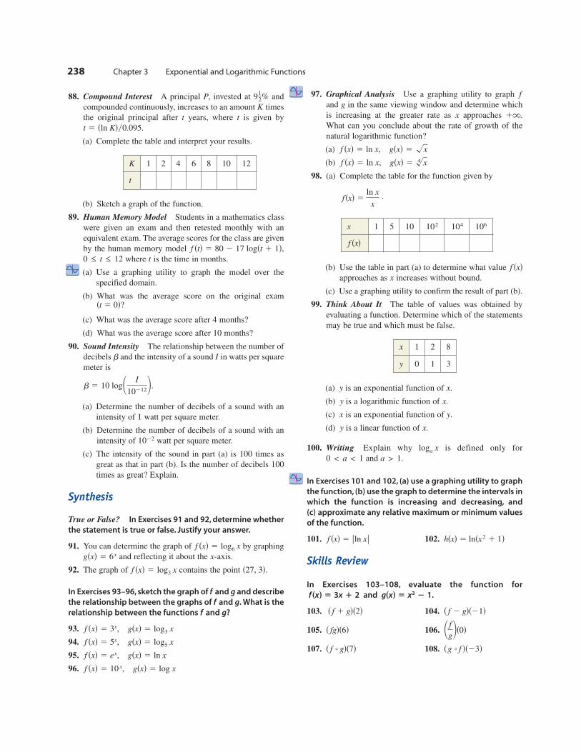
89. Human Memory Model Students in a mathematics class
were given an exam and then retested monthly with an
equivalent exam. The average scores for the class are given
by the human memory model
where is the time in months.
(a) Use a graphing utility to graph the model over the
specified domain.
(b) What was the average score on the original exam
(c) What was the average score after 4 months?
(d) What was the average score after 10 months?
90. Sound Intensity The relationship between the number of
decibels and the intensity of a sound in watts per square
meter is
(a) Determine the number of decibels of a sound with an
intensity of 1 watt per square meter.
(b) Determine the number of decibels of a sound with an
intensity of watt per square meter.
(c) The intensity of the sound in part (a) is 100 times as
great as that in part (b). Is the number of decibels 100
times as great? Explain.
Synthesis
True or False? In Exercises 91 and 92, determine whether
the statement is true or false. Justify your answer.
91. You can determine the graph of by graphing
and reflecting it about the -axis.
92. The graph of contains the point
In Exercises 93–96, sketch the graph of and and describe
the relationship between the graphs of and What is the
relationship between the functions and
93.
94.
95.
96.
97. Graphical Analysis Use a graphing utility to graph
and in the same viewing window and determine which
is increasing at the greater rate as approaches
What can you conclude about the rate of growth of the
natural logarithmic function?
(a)
(b)
98. (a) Complete the table for the function given by
(b) Use the table in part (a) to determine what value
approaches as increases without bound.
(c) Use a graphing utility to confirm the result of part (b).
99. Think About It The table of values was obtained by
evaluating a function. Determine which of the statements
may be true and which must be false.
(a) is an exponential function of
(b) is a logarithmic function of
(c) is an exponential function of
(d) is a linear function of
100. Writing Explain why is defined only for
and
In Exercises 101 and 102, (a) use a graphing utility to graph
the function, (b) use the graph to determine the intervals in
which the function is increasing and decreasing, and
(c) approximate any relative maximum or minimum values
of the function.
101. 102.
Skills Review
In Exercises 103–108, evaluate the function for
and
103. 104.
105. 106.
107. 108. sg 8 f ds23ds f 8 gds7d
1 f
g2s0ds fgds6d
s f 2 gds21ds f 1 gds2d
gxxc 5 x32 1.f xxc 5 3x 1 2
hsxd 5 lnsx2 1 1df sxd 5 |ln x|
a > 1.0 < a < 1
loga x
x.y
y.x
x.y
x.y
x
f sxd
fsxd 5ln x
x .
gsxd 5 4!xf sxd 5 ln x,
gsxd 5 !xf sxd 5 ln x,
1 .̀x
g
f
gsxd 5 log xf sxd 5 10 x,
gsxd 5 ln xf sxd 5 ex,
gsxd 5 log5 xf sxd 5 5x,
gsxd 5 log3 xf sxd 5 3x,
g?f
g.f
gf
s27, 3d.f sxd 5 log3 x
xgsxd 5 6x
f sxd 5 log6 x
1022
b 5 10 log1 I
102122.
Ib
st 5 0d?
t0 ≤ t ≤ 12
f std 5 80 2 17 logst 1 1d,
t 5 sln Kdy0.095.
tt
K
912%P,
238 Chapter 3 Exponential and Logarithmic Functions
x 1 5 10
f sxd
106104102
x 1 2 8
y 0 1 3
K 1 2 4 6 8 10 12
t
Section 3.3 Properties of Logarithms 239
Change of Base
Most calculators have only two types of log keys, one for common logarithms
(base 10) and one for natural logarithms (base ). Although common logs and
natural logs are the most frequently used, you may occasionally need to evaluate
logarithms to other bases. To do this, you can use the following change-of-base
formula.
One way to look at the change-of-base formula is that logarithms to base
are simply constant multiples of logarithms to base The constant multiplier is
Changing Bases Using Common Logarithms
a.
Use a calculator.
Simplify.
b.
Now try Exercise 1(a).
Changing Bases Using Natural Logarithms
a.
Use a calculator.
Simplify.
b.
Now try Exercise 1(b).
log2 12 5ln 12
ln 2<
2.48491
0.69315< 3.5850
< 2.3219
<3.21888
1.38629
loga x 5ln x
ln a log4 25 5
ln 25
ln 4
log2 12 5log 12
log 2<
1.07918
0.30103< 3.5850
< 2.3219
<1.39794
0.60206
loga x 5log x
log a log4 25 5
log 25
log 4
1yslogbad.b.
a
e
What you should learn
• Use the change-of-base
formula to rewrite and evalu-
ate logarithmic expressions.
• Use properties of logarithms
to evaluate or rewrite logarith-
mic expressions.
• Use properties of logarithms
to expand or condense
logarithmic expressions.
• Use logarithmic functions
to model and solve real-life
problems.
Why you should learn it
Logarithmic functions can be
used to model and solve real-life
problems. For instance, in
Exercises 81–83 on page 244, a
logarithmic function is used to
model the relationship between
the number of decibels and the
intensity of a sound.
Properties of Logarithms
AP Photo/Stephen Chernin
3.3
Change-of-Base Formula
Let and be positive real numbers such that and Then
can be converted to a different base as follows.
Base b Base 10 Base e
loga x 5ln x
ln aloga x 5
log x
log aloga x 5
logb x
logb a
loga x
b Þ 1.a Þ 1xb,a,
Example 1
Example 2
Properties of Logarithms
You know from the preceding section that the logarithmic function with base
is the inverse function of the exponential function with base So, it makes sense
that the properties of exponents should have corresponding properties involving
logarithms. For instance, the exponential property has the corresponding
logarithmic property
For proofs of the properties listed above, see Proofs in Mathematics on page
278.
Using Properties of Logarithms
Write each logarithm in terms of ln 2 and ln 3.
a. ln 6 b.
Solution
a. Rewrite 6 as
Product Property
b. Quotient Property
Rewrite 27 as
Power Property
Now try Exercise 17.
Using Properties of Logarithms
Find the exact value of each expression without using a calculator.
a. b.
Solution
a.
b.
Now try Exercise 23.
ln e6 2 ln e2 5 lne6
e25 ln e4 5 4 ln e 5 4s1d 5 4
log5 3!5 5 log5 5
1y3 513 log5 5 5
13 s1d 5
13
ln e6 2 ln e2log5 3!5
5 ln 2 2 3 ln 3
33. 5 ln 2 2 ln 33
ln2
275 ln 2 2 ln 27
5 ln 2 1 ln 3
2 ? 3.ln 6 5 lns2 ? 3d
ln 2
27
loga1 5 0.
a0 5 1
a.
a
240 Chapter 3 Exponential and Logarithmic Functions
There is no general property
that can be used to rewrite
Specifically,
is not equal to
loga u 1 loga v.
logasu 1 vdlogasu ± vd.
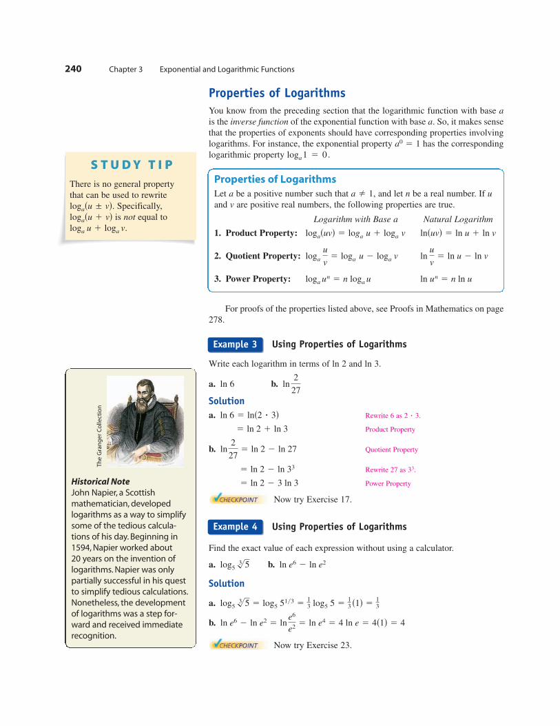
Historical Note
John Napier, a Scottish
mathematician, developed
logarithms as a way to simplify
some of the tedious calcula-
tions of his day. Beginning in
1594, Napier worked about
20 years on the invention of
logarithms. Napier was only
partially successful in his quest
to simplify tedious calculations.
Nonetheless, the development
of logarithms was a step for-
ward and received immediate
recognition.
Th
e G
ran
ge
r C
olle
ctio
n
Properties of Logarithms
Let be a positive number such that and let be a real number. If
and are positive real numbers, the following properties are true.
Logarithm with Base a Natural Logarithm
1. Product Property:
2. Quotient Property:
3. Power Property: ln un 5 n ln uloga un 5 n loga u
ln u
v5 ln u 2 ln vloga
u
v5 loga u 2 loga v
lnsuvd 5 ln u 1 ln vlogasuvd 5 loga u 1 loga v
v
una Þ 1,a
Example 3
Example 4
Rewriting Logarithmic Expressions
The properties of logarithms are useful for rewriting logarithmic expressions in
forms that simplify the operations of algebra. This is true because these proper-
ties convert complicated products, quotients, and exponential forms into simpler
sums, differences, and products, respectively.
Expanding Logarithmic Expressions
Expand each logarithmic expression.
a. b.
Solution
a. Product Property
Power Property
b.
Quotient Property
Power Property
Now try Exercise 47.
In Example 5, the properties of logarithms were used to expand logarithmic
expressions. In Example 6, this procedure is reversed and the properties of loga-
rithms are used to condense logarithmic expressions.
Condensing Logarithmic Expressions
Condense each logarithmic expression.
a. b.
c.
Solution
a. Power Property
Product Property
b. Power Property
Quotient Property
c. Product Property
Power Property
Rewrite with a radical.
Now try Exercise 69.
5 log2 3!xsx 1 1d
5 log2fxsx 1 1dg1y3
13 flog2 x 1 log2sx 1 1dg 5
13Hlog2fxsx 1 1dgJ
5 ln sx 1 2d2
x
2 lnsx 1 2d 2 ln x 5 lnsx 1 2d2 2 ln x
5 logf!xsx 1 1d3g 12 log x 1 3 logsx 1 1d 5 log x
1y2 1 logsx 1 1d3
13 flog2 x 1 log2sx 1 1dg
2 lnsx 1 2d 2 ln x12 log x 1 3 logsx 1 1d
51
2 lns3x 2 5d 2 ln 7
5 lns3x 2 5d1y2 2 ln 7
ln !3x 2 5
75 ln
s3x 2 5d1y2
7
5 log4 5 1 3 log4 x 1 log4 y
log4 5x3y 5 log4 5 1 log4 x3 1 log4 y
ln !3x 2 5
7log4 5x3y
Section 3.3 Properties of Logarithms 241
Use a graphing utility to graph
the functions given by
and
in the same viewing window.
Does the graphing utility show
the functions with the same
domain? If so, should it?
Explain your reasoning.
y2 5 ln x
x 2 3
y1 5 ln x 2 lnsx 2 3d
Exploration
Rewrite using rationalexponent.
Example 5
Example 6
242 Chapter 3 Exponential and Logarithmic FunctionsP
erio
d (
in y
ears
)
Mean distance
(in astronomical units)
5
10
15
20
25
30
4 6 8 10x
y
Mercury
Earth
Venus
Mars
Jupiter
Saturn
Planets Near the Sun
2
FIGURE 3.23
ln x
Venus
EarthMars
Jupiter
Saturn
31 2
1
2
3
ln y = ln x3
2
ln y
Mercury
FIGURE 3.24
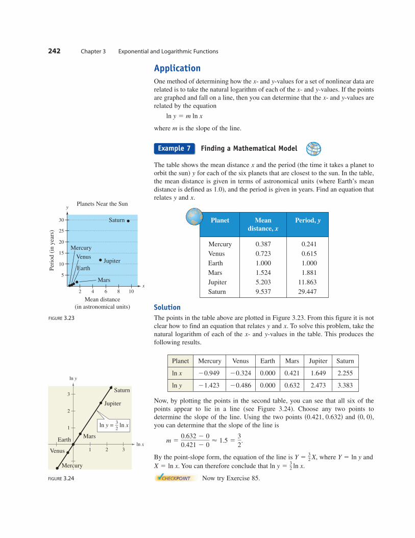
Application
One method of determining how the - and -values for a set of nonlinear data are
related is to take the natural logarithm of each of the - and -values. If the points
are graphed and fall on a line, then you can determine that the - and -values are
related by the equation
where is the slope of the line.
Finding a Mathematical Model
The table shows the mean distance and the period (the time it takes a planet to
orbit the sun) for each of the six planets that are closest to the sun. In the table,
the mean distance is given in terms of astronomical units (where Earth’s mean
distance is defined as 1.0), and the period is given in years. Find an equation that
relates and
Solution
The points in the table above are plotted in Figure 3.23. From this figure it is not
clear how to find an equation that relates and To solve this problem, take the
natural logarithm of each of the - and -values in the table. This produces the
following results.
Now, by plotting the points in the second table, you can see that all six of the
points appear to lie in a line (see Figure 3.24). Choose any two points to
determine the slope of the line. Using the two points and
you can determine that the slope of the line is
By the point-slope form, the equation of the line is where and
You can therefore conclude that
Now try Exercise 85.
ln y 532 ln x.X 5 ln x.
Y 5 ln yY 532 X,
m 50.632 2 0
0.421 2 0< 1.5 5
3
2.
s0, 0d,s0.421, 0.632d
yx
x.y
x.y
y
x
m
ln y 5 m ln x
yx
yx
yx
Planet Mercury Venus Earth Mars Jupiter Saturn
0.000 0.421 1.649 2.255
0.000 0.632 2.473 3.38320.48621.423ln y
20.32420.949ln x
Planet Mean Period, y
distance, x
Mercury 0.387 0.241
Venus 0.723 0.615
Earth 1.000 1.000
Mars 1.524 1.881
Jupiter 5.203 11.863
Saturn 9.537 29.447
Example 7

Section 3.3 Properties of Logarithms 243
Exercises 3.3
In Exercises 1–8, rewrite the logarithm as a ratio of (a) com-
mon logarithms and (b) natural logarithms.
1. 2.
3. 4.
5. 6.
7. 8.
In Exercises 9–16, evaluate the logarithm using the
change-of-base formula. Round your result to three
decimal places.
9. 10.
11. 12.
13. 14.
15. 16.
In Exercises 17–22, use the properties of logarithms to
rewrite and simplify the logarithmic expression.
17. 18.
19. 20.
21. 22.
In Exercises 23–38, find the exact value of the logarithmic
expression without using a calculator. (If this is not possi-
ble, state the reason.)
23. 24.
25. 26.
27. 28.
29. 30.
31.
32.
33.
34.
35.
36.
37.
38.
In Exercises 39–60, use the properties of logarithms to
expand the expression as a sum, difference, and/or constant
multiple of logarithms. (Assume all variables are positive.)
39. 40.
41. 42.
43. 44.
45. 46.
47. 48.
49. 50.
51. 52.
53. 54.
55. 56.
57. 58.
59. 60. ln!x2sx 1 2dln 4!x3sx21 3d
log10 xy4
z5log5
x2
y2z3
log2 !x y4
z4ln
x4!y
z5
ln!x2
y3ln 3!x
y
ln 6
!x21 1
log2
!a 2 1
9, a > 1
ln1x22 1
x3 2, x > 1ln zsz 2 1d2, z > 1
log 4x2 yln xyz2
ln 3!tln !z
log6 1
z3log5
5
x
log10 y
2log8 x
4
log3 10zlog4 5x
log4 2 1 log4 32
log5 75 2 log5 3
2 ln e62 ln e5
ln e21 ln e5
ln 4!e3
ln 1
!e
3 ln e4
ln e4.5
log2s216dlog3s29dlog3 8120.2log4 161.2
log6 3!6log2
4!8
log5 1
125log3 9
ln 6
e2lns5e6d
log 9
300log5 1
250
log2s42? 34dlog4 8
log3 0.015log15 1250
log20 0.125log9 0.4
log1y4 5log1y2 4
log7 4log3 7
log7.1 xlog2.6 x
logx 34logx
310
log1y3 xlog1y5 x
log3 xlog5 x
VOCABULARY CHECK:
In Exercises 1 and 2, fill in the blanks.
1. To evaluate a logarithm to any base, you can use the ________ formula.
2. The change-of-base formula for base is given by ________.
In Exercises 3–5, match the property of logarithms with its name.
3. (a) Power Property
4. (b) Quotient Property
5. (c) Product Property
PREREQUISITE SKILLS REVIEW: Practice and review algebra skills needed for this section at www.Eduspace.com.
loga
u
v5 loga u 2 loga v
ln un5 n ln u
logasuvd 5 loga u 1 loga v
loga x 5e
In Exercises 61–78, condense the expression to the
logarithm of a single quantity.
61.
62.
63.
64.
65.
66.
67.
68.
69.
70.
71.
72.
73.
74.
75.
76.
77.
78.
In Exercises 79 and 80, compare the logarithmic quantities.
If two are equal, explain why.
79.
80.
Sound Intensity In Exercises 81–83, use the following
information. The relationship between the number of deci-
bels and the intensity of a sound in watts per square
meter is given by
81. Use the properties of logarithms to write the formula in
simpler form, and determine the number of decibels of a
sound with an intensity of watt per square meter.
82. Find the difference in loudness between an average office
with an intensity of watt per square meter and
a broadcast studio with an intensity of watt
per square meter.
83. You and your roommate are playing your stereos at the
same time and at the same intensity. How much louder is
the music when both stereos are playing compared with
just one stereo playing?
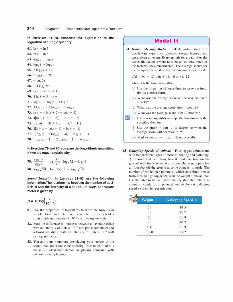
85. Galloping Speeds of Animals Four-legged animals run
with two different types of motion: trotting and galloping.
An animal that is trotting has at least one foot on the
ground at all times, whereas an animal that is galloping has
all four feet off the ground at some point in its stride. The
number of strides per minute at which an animal breaks
from a trot to a gallop depends on the weight of the animal.
Use the table to find a logarithmic equation that relates an
animal’s weight (in pounds) and its lowest galloping
speed (in strides per minute).y
x
3.16 3 1025
1.26 3 1027
1026
b 5 10 log_ I
10212+.
Ib
log7!70, log7 35, 12 1 log7 !10
log2 32
log2 4, log2
32
4, log2 32 2 log2 4
12flog4sx 1 1d 1 2 log4sx 2 1dg 1 6 log4 x
13flog8 y 1 2 log8sy 1 4dg 2 log8sy 2 1d2f3 ln x 2 lnsx 1 1d 2 lnsx 2 1dg
13f2 lnsx 1 3d 1 ln x 2 lnsx2
2 1dg4fln z 1 lnsz 1 5dg 2 2 lnsz 2 5dln x 2 4flnsx 1 2d 1 lnsx 2 2dg3 log3 x 1 4 log3 y 2 4 log3 z
log x 2 2 log y 1 3 log z
2 ln 8 1 5 lnsz 2 4dln x 2 3 lnsx 1 1d24 log6 2x
14 log3 5x
23 log7sz 2 2d2 log2sx 1 4dlog5 8 2 log5 t
log4 z 2 log4 y
ln y 1 ln t
ln x 1 ln 3
244 Chapter 3 Exponential and Logarithmic Functions
84. Human Memory Model Students participating in a
psychology experiment attended several lectures and
were given an exam. Every month for a year after the
exam, the students were retested to see how much of
the material they remembered. The average scores for
the group can be modeled by the human memory model
where is the time in months.
(a) Use the properties of logarithms to write the func-
tion in another form.
(b) What was the average score on the original exam
(c) What was the average score after 4 months?
(d) What was the average score after 12 months?
(e) Use a graphing utility to graph the function over the
specified domain.
(f) Use the graph in part (e) to determine when the
average score will decrease to 75.
(g) Verify your answer to part (f) numerically.
st 5 0d?
t
0 ≤ t ≤ 12f std 5 90 2 15 logst 1 1d,
Model It
Weight, x Galloping Speed, y
25 191.5
35 182.7
50 173.8
75 164.2
500 125.9
1000 114.2
Section 3.3 Properties of Logarithms 245
86. Comparing Models A cup of water at an initial tempera-
ture of is placed in a room at a constant temperature
of The temperature of the water is measured every 5
minutes during a half-hour period. The results are record-
ed as ordered pairs of the form where is the time (in
minutes) and is the temperature (in degrees Celsius).
(a) The graph of the model for the data should be
asymptotic with the graph of the temperature of the
room. Subtract the room temperature from each of the
temperatures in the ordered pairs. Use a graphing
utility to plot the data points and
(b) An exponential model for the data is given
by
Solve for and graph the model. Compare the result
with the plot of the original data.
(c) Take the natural logarithms of the revised temperatures.
Use a graphing utility to plot the points
and observe that the points appear to be linear. Use the
regression feature of the graphing utility to fit a line to
these data. This resulting line has the form
Use the properties of the logarithms to solve for
Verify that the result is equivalent to the model in
part (b).
(d) Fit a rational model to the data. Take the reciprocals of
the -coordinates of the revised data points to generate
the points
Use a graphing utility to graph these points and observe
that they appear to be linear. Use the regression feature
of a graphing utility to fit a line to these data. The
resulting line has the form
Solve for and use a graphing utility to graph the
rational function and the original data points.
(e) Write a short paragraph explaining why the transforma-
tions of the data were necessary to obtain each model.
Why did taking the logarithms of the temperatures lead
to a linear scatter plot? Why did taking the reciprocals
of the temperature lead to a linear scatter plot?
Synthesis
True or False? In Exercises 87–92, determine whether the
statement is true or false given that Justify your
answer.
87.
88.
89.
90.
91. If then
92. If then
93. Proof Prove that
94. Proof Prove that
In Exercises 95–100, use the change -of-base formula to
rewrite the logarithm as a ratio of logarithms. Then use a
graphing utility to graph both functions in the same
viewing window to verify that the functions are equivalent.
95. 96.
97. 98.
99. 100.
101. Think About It Consider the functions below.
Which two functions should have identical graphs? Verify
your answer by sketching the graphs of all three functions
on the same set of coordinate axes.
102. Exploration For how many integers between 1 and 20
can the natural logarithms be approximated given that
and
Approximate these logarithms (do not use a calculator).
Skills Review
In Exercises 103–106, simplify the expression.
103. 104.
105. 106.
In Exercises 107–110, solve the equation.
107. 108.
109. 110.5
x 2 15
2x
3
2
3x 1 15
x
4
4x2 2 5x 1 1 5 03x2 1 2x 2 1 5 0
xysx21 1 y21d21s18x3y4d23s18x3y4d3
12x2
3y 22324xy22
16x23y
1.6094?ln 5 <ln 2 < 0.6931, ln 3 < 1.0986,
f sxd 5 ln x
2, gsxd 5
ln x
ln 2, hsxd 5 ln x 2 ln 2
f sxd 5 log12.4 xf sxd 5 log11.8 x
f sxd 5 log1y4 xf sxd 5 log1y2 x
f sxd 5 log4 xf sxd 5 log2 x
logb un 5 n logb u.
logb u
v5 logb u 2 logb v.
0 < x < 1.f sxd < 0,
v 5 u2.f sud 5 2 f svd,!f sxd 5
12 f sxd
x > 2f sx 2 2d 5 f sxd 2 f s2d,a > 0, x > 0f saxd 5 f sad 1 f sxd,
f s0d 5 0
f xxc 5 ln x.
T,
1
T 2 215 at 1 b.
1t, 1
T 2 212.
y
T.
lnsT 2 21d 5 at 1 b.
st, lnsT 2 21dd
T
T 2 21 5 54.4s0.964dt.
st, T 2 21dst, T 2 21d.st, Td
s30, 39.68ds25, 42.48d,s20, 46.38d,s15, 51.28d,s10, 57.58d,s5, 66.08d,s0, 78.08d,
T
tst, Td,
218 C.
788 C

Introduction
So far in this chapter, you have studied the definitions, graphs, and properties of
exponential and logarithmic functions. In this section, you will study procedures
for solving equations involving these exponential and logarithmic functions.
There are two basic strategies for solving exponential or logarithmic
equations. The first is based on the One-to-One Properties and was used to solve
simple exponential and logarithmic equations in Sections 3.1 and 3.2. The
second is based on the Inverse Properties. For and the following
properties are true for all and for which and are defined.
One-to-One Properties
if and only if
if and only if
Inverse Properties
Solving Simple Equations
Original Rewritten
Equation Equation Solution Property
a. One-to-One
b. One-to-One
c. One-to-One
d. Inverse
e. Inverse
f. Inverse
Now try Exercise 13.
The strategies used in Example 1 are summarized as follows.
x 5 1021 511010 log x 5 1021log x 5 21
x 5 e23e ln x 5 e23ln x 5 23
x 5 ln 7ln e x 5 ln 7e x 5 7
x 5 2232x 5 32s13dx
5 9
x 5 3ln x 5 ln 3ln x 2 ln 3 5 0
x 5 52x 5 252x 5 32
loga ax 5 x
aloga x 5 x
x 5 y.loga x 5 loga y
x 5 y.a x 5 a y
loga yloga xyx
a Þ 1,a > 0
246 Chapter 3 Exponential and Logarithmic Functions
What you should learn
• Solve simple exponential
and logarithmic equations.
• Solve more complicated
exponential equations.
• Solve more complicated
logarithmic equations.
• Use exponential and logarith-
mic equations to model and
solve real-life problems.
Why you should learn it
Exponential and logarithmic
equations are used to model
and solve life science applica-
tions. For instance, in Exercise
112, on page 255, a logarithmic
function is used to model the
number of trees per acre given
the average diameter of the
trees.
Exponential and Logarithmic Equations
© James Marshall/Corbis
3.4
Strategies for Solving Exponential and LogarithmicEquations
1. Rewrite the original equation in a form that allows the use of the
One-to-One Properties of exponential or logarithmic functions.
2. Rewrite an exponential equation in logarithmic form and apply the
Inverse Property of logarithmic functions.
3. Rewrite a logarithmic equation in exponential form and apply the Inverse
Property of exponential functions.
Example 1
Solving Exponential Equations
Solving Exponential Equations
Solve each equation and approximate the result to three decimal places if
necessary.
a. b.
Solution
a. Write original equation.
One-to-One Property
Write in general form.
Factor.
Set 1st factor equal to 0.
Set 2nd factor equal to 0.
The solutions are and Check these in the original equation.
b. Write original equation.
Divide each side by 3.
Take log (base 2) of each side.
Inverse Property
Change-of-base formula
The solution is Check this in the original equation.
Now try Exercise 25.
In Example 2(b), the exact solution is and the approximate
solution is An exact answer is preferred when the solution is an
intermediate step in a larger problem. For a final answer, an approximate solution
is easier to comprehend.
Solving an Exponential Equation
Solve and approximate the result to three decimal places.
Solution
Write original equation.
Subtract 5 from each side.
Take natural log of each side.
Inverse Property
The solution is ln 55 . Check this in the original equation.
Now try Exercise 51.
< 4.007x 5
x 5 ln 55 < 4.007
ln ex 5 ln 55
e x 5 55
e x 1 5 5 60
e x 1 5 5 60
x < 3.807.
x 5 log2 14
x 5 log2 14 < 3.807.
x 5ln 14
ln 2< 3.807
x 5 log2 14
log2 2x 5 log2 14
2 x 5 14
3s2 xd 5 42
x 5 4.x 5 21
sx 2 4d 5 0 ⇒ x 5 4
sx 1 1d 5 0 ⇒ x 5 21
sx 1 1dsx 2 4d 5 0
x2 2 3x 2 4 5 0
2x2 5 23x 2 4
e2x2
5 e23x24
3s2 xd 5 42e2x25 e23x24
Section 3.4 Exponential and Logarithmic Equations 247
Remember that the natural loga-
rithmic function has a base of e.
Example 2
Example 3

Solving an Exponential Equation
Solve and approximate the result to three decimal places.
Solution
Write original equation.
Add 4 to each side.
Divide each side by 2.
Take log (base 3) of each side.
Inverse Property
Add 5 to each side.
Divide each side by 2.
Use a calculator.
The solution is Check this in the original equation.
Now try Exercise 53.
When an equation involves two or more exponential expressions, you can
still use a procedure similar to that demonstrated in Examples 2, 3, and 4.
However, the algebra is a bit more complicated.
t 552 1
12 log3 7.5 < 3.417.
t < 3.417
t 55
21
1
2 log3 7.5
2t 5 5 1 log3 7.5
2t 2 5 5 log3 15
2
log3 32t25 5 log3
15
2
32t25 515
2
2s32t25d 5 15
2s32t25d 2 4 5 11
2s32t25d 2 4 5 11
248 Chapter 3 Exponential and Logarithmic Functions
Example 4
Remember that to evaluate a
logarithm such as you
need to use the change-of-base
formula.
log3 7.5 5ln 7.5
ln 3< 1.834
log3 7.5,
Solving an Exponential Equation of Quadratic Type
Solve e2x 2 3e x 1 2 5 0.
Example 5
Algebraic Solution
Write original equation.
Write in quadratic form.
Factor.
Set 1st factor equal to 0.
Solution
Set 2nd factor equal to 0.
Solution
The solutions are and Check
these in the original equation.
Now try Exercise 67.
x 5 0.x 5 ln 2 < 0.693
x 5 0
e x 2 1 5 0
x 5 ln 2
e x 2 2 5 0
se x 2 2dse x 2 1d 5 0
se xd2 2 3e x 1 2 5 0
e2x 2 3e x 1 2 5 0
Graphical Solution
Use a graphing utility to graph Use the
zero or root feature or the zoom and trace features of the
graphing utility to approximate the values of for which
In Figure 3.25, you can see that the zeros occur at
and at So, the solutions are and
FIGURE 3.25
3
−1
3
3y = e2x − 3ex + 2
x < 0.693.
x 5 0x < 0.693.x 5 0
y 5 0.
x
y 5 e2x 2 3ex 1 2.

Solving Logarithmic Equations
To solve a logarithmic equation, you can write it in exponential form.
Logarithmic form
Exponentiate each side.
Exponential form
This procedure is called exponentiating each side of an equation.
Solving Logarithmic Equations
a. Original equation
Exponentiate each side.
Inverse Property
b. Original equation
One-to-One Property
Add and 1 to each side.
Divide each side by 4.
c. Original equation
Quotient Property of Logarithms
One-to-One Property
Cross multiply.
Isolate
Divide each side by
Now try Exercise 77.
Solving a Logarithmic Equation
Solve and approximate the result to three decimal places.
Solution
Write original equation.
Subtract 5 from each side.
Divide each side by 2.
Exponentiate each side.
Inverse Property
Use a calculator.
Now try Exercise 85.
x < 0.607
x 5 e21y2
eln x 5 e21y2
ln x 5 21
2
2 ln x 5 21
5 1 2 ln x 5 4
5 1 2 ln x 5 4
27. x 5 2
x. 27x 5 214
3x 1 14 5 10x
3x 1 14
55 2x
log613x 1 14
5 2 5 log6 2x
log6s3x 1 14d 2 log6 5 5 log6 2x
x 5 2
2x 4x 5 8
5x 2 1 5 x 1 7
log3s5x 2 1d 5 log3sx 1 7d
x 5 e2
e ln x 5 e2
ln x 5 2
x 5 e3
eln x 5 e3
ln x 5 3
Section 3.4 Exponential and Logarithmic Equations 249
Example 6
Example 7
Remember to check your solu-
tions in the original equation
when solving equations to verify
that the answer is correct and to
make sure that the answer lies
in the domain of the original
equation.
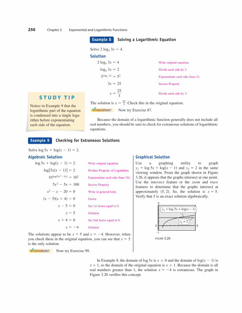
Solving a Logarithmic Equation
Solve 2
Solution
Write original equation.
Divide each side by 2.
Exponentiate each side (base 5).
Inverse Property
Divide each side by 3.
The solution is Check this in the original equation.
Now try Exercise 87.
Because the domain of a logarithmic function generally does not include all
real numbers, you should be sure to check for extraneous solutions of logarithmic
equations.
x 5253 .
x 525
3
3x 5 25
5 log5 3x 5 52
log5 3x 5 2
2 log5 3x 5 4
log5 3x 5 4.
250 Chapter 3 Exponential and Logarithmic Functions
Example 8
Notice in Example 9 that the
logarithmic part of the equation
is condensed into a single loga-
rithm before exponentiating
each side of the equation.
In Example 9, the domain of is and the domain of is
so the domain of the original equation is Because the domain is all
real numbers greater than 1, the solution is extraneous. The graph in
Figure 3.26 verifies this concept.
x 5 24
x > 1.x > 1,
logsx 2 1dx > 0log 5x
Checking for Extraneous Solutions
Solve log 5x 1 logsx 2 1d 5 2.
Example 9
Algebraic Solution
Write original equation.
Product Property of Logarithms
Exponentiate each side (base 10).
Inverse Property
Write in general form.
Factor.
Set 1st factor equal to 0.
Solution
Set 2nd factor equal to 0.
Solution
The solutions appear to be and However, when
you check these in the original equation, you can see that
is the only solution.
Now try Exercise 99.
x 5 5
x 5 24.x 5 5
x 5 24
x 1 4 5 0
x 5 5
x 2 5 5 0
sx 2 5dsx 1 4d 5 0
x2 2 x 2 20 5 0
5x2 2 5x 5 100
10 logs5x225xd 5 102
logf5xsx 2 1dg 5 2
log 5x 1 logsx 2 1d 5 2
Graphical Solution
Use a graphing utility to graph
and in the same
viewing window. From the graph shown in Figure
3.26, it appears that the graphs intersect at one point.
Use the intersect feature or the zoom and trace
features to determine that the graphs intersect at
approximately So, the solution is
Verify that 5 is an exact solution algebraically.
FIGURE 3.26
0
−1
9
y1 = log 5x + log(x − 1)
y2 = 2
5
x 5 5.s5, 2d.
y2 5 2y1 5 log 5x 1 logsx 2 1d

Applications
Doubling an Investment
You have deposited $500 in an account that pays 6.75% interest, compounded
continuously. How long will it take your money to double?
Solution
Using the formula for continuous compounding, you can find that the balance in
the account is
To find the time required for the balance to double, let and solve the
resulting equation for
Let
Divide each side by 500.
Take natural log of each side.
Inverse Property
Divide each side by 0.0675.
Use a calculator.
The balance in the account will double after approximately 10.27 years. This
result is demonstrated graphically in Figure 3.27.
FIGURE 3.27
Now try Exercise 107.
In Example 10, an approximate answer of 10.27 years is given. Within the
context of the problem, the exact solution, years, does not make
sense as an answer.
sln 2dy0.0675
t
Time (in years)
(0, 500)
(10.27, 1000)
Acc
ount
bal
ance
(in
doll
ars)
100
300
500
700
900
1100
108642
A
THE UNITED STATES OF AMERICA
THE UNITED STATES OF AMERICA
THE UNITED STATES OF AMERICA
WA
SHIN
GTON
WASHINGTON, D.C.
AC 4
C 31
1
1
1
1SERIES
1993
Doubling an Investment
A = 500e0.0675t
t < 10.27
t 5ln 2
0.0675
0.0675t 5 ln 2
ln e0.0675t 5 ln 2
e0.0675t 5 2
A 5 1000. 500e0.0675t 5 1000
t.
A 5 1000
A 5 500e0.0675t.
A 5 Pert
Section 3.4 Exponential and Logarithmic Equations 251
Example 10
The effective yield of a savings
plan is the percent increase in
the balance after 1 year. Find
the effective yield for each
savings plan when $1000 is
deposited in a savings account.
a. 7% annual interest rate,
compounded annually
b. 7% annual interest rate,
compounded continuously
c. 7% annual interest rate,
compounded quarterly
d. 7.25% annual interest rate,
compounded quarterly
Which savings plan has the
greatest effective yield? Which
savings plan will have the
highest balance after 5 years?
Exploration
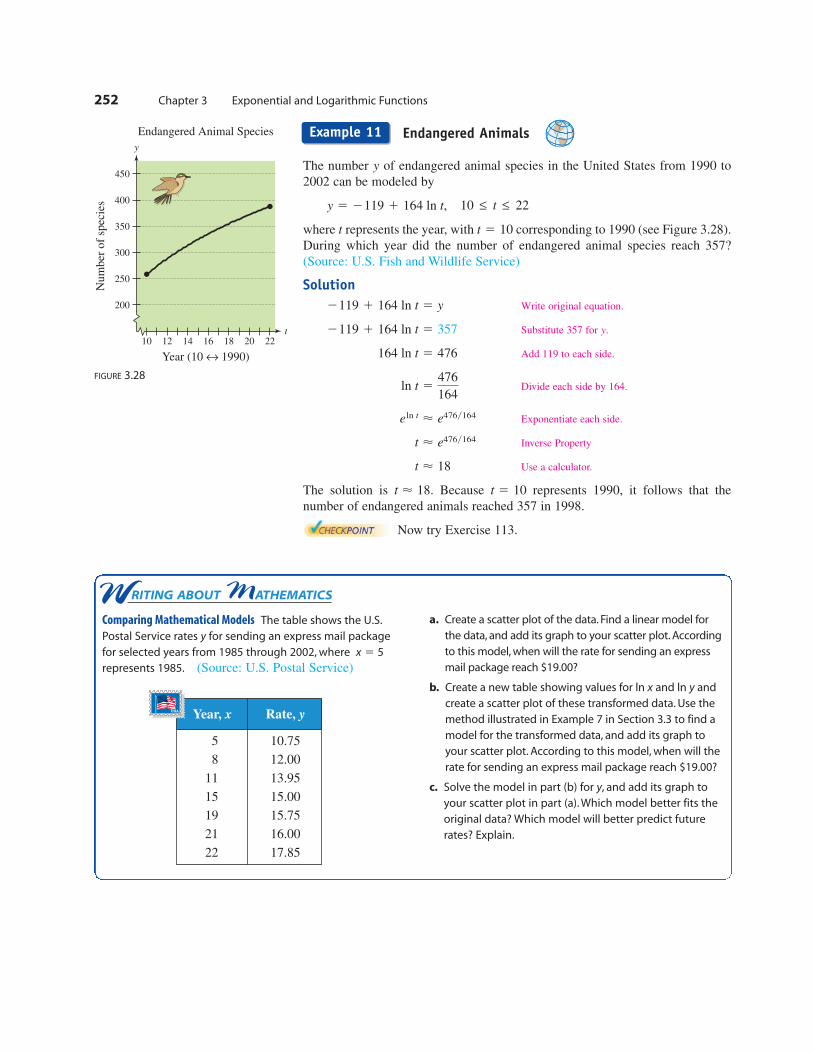
W RITING ABOUT MATHEMATICS
Endangered Animals
The number of endangered animal species in the United States from 1990 to
2002 can be modeled by
where represents the year, with corresponding to 1990 (see Figure 3.28).
During which year did the number of endangered animal species reach 357?
(Source: U.S. Fish and Wildlife Service)
Solution
Write original equation.
Substitute 357 for
Add 119 to each side.
Divide each side by 164.
Exponentiate each side.
Inverse Property
Use a calculator.
The solution is Because represents 1990, it follows that the
number of endangered animals reached 357 in 1998.
Now try Exercise 113.
t 5 10t < 18.
t < 18
t < e476y164
eln t < e476y164
ln t 5476
164
164 ln t 5 476
y. 2119 1 164 ln t 5 357
2119 1 164 ln t 5 y
t 5 10t
10 ≤ t ≤ 22y 5 2119 1 164 ln t,
y
252 Chapter 3 Exponential and Logarithmic Functions
Example 11
10 12 14 16 18 20 22
200
250
300
350
400
450
t
y
Endangered Animal Species
Num
ber
of
spec
ies
Year (10 ↔ 1990)
FIGURE 3.28
Comparing Mathematical Models The table shows the U.S.
Postal Service rates y for sending an express mail package
for selected years from 1985 through 2002, where
represents 1985. (Source: U.S. Postal Service)
a. Create a scatter plot of the data. Find a linear model for
the data, and add its graph to your scatter plot. According
to this model, when will the rate for sending an express
mail package reach $19.00?
b. Create a new table showing values for ln x and ln y and
create a scatter plot of these transformed data. Use the
method illustrated in Example 7 in Section 3.3 to find a
model for the transformed data, and add its graph to
your scatter plot. According to this model, when will the
rate for sending an express mail package reach $19.00?
c. Solve the model in part (b) for y, and add its graph to
your scatter plot in part (a). Which model better fits the
original data? Which model will better predict future
rates? Explain.
x 5 5
Year, x Rate, y
5 10.75
8 12.00
11 13.95
15 15.00
19 15.75
21 16.00
22 17.85

Section 3.4 Exponential and Logarithmic Equations 253
Exercises 3.4
In Exercises 1–8, determine whether each -value is a
solution (or an approximate solution) of the equation.
1. 2.
(a) (a)
(b) (b)
3.
(a)
(b)
(c)
4.
(a)
(b)
(c)
5.
(a)
(b)
(c)
6.
(a)
(b)
(c)
7.
(a)
(b)
(c)
8.
(a)
(b)
(c)
In Exercises 9–20, solve for
9. 10.
11. 12.
13. 14.
15. 16.
17. 18.
19. 20.
In Exercises 21–24, approximate the point of intersection
of the graphs of and Then solve the equation
algebraically to verify your approximation.
21. 22.
23. 24.
x
−4
8 12
4
8
12
fg
y
xf
g
y
4 8 12
4
gsxd 5 0gsxd 5 2
f sxd 5 lnsx 2 4df sxd 5 log3 x
x−8 −4
−4
4 8
4
8
12
f
g
y
x−8 −4
−4
4 8
4
12
f
g
y
gsxd 5 9gsxd 5 8
f sxd 5 27xf sxd 5 2x
f xxc 5 gxxcg.f
log5 x 5 23log4 x 5 3
ln x 5 27ln x 5 21
ex 5 4ex 5 2
ln x 2 ln 5 5 0ln x 2 ln 2 5 0
s14dx
5 64s12dx
5 32
3x 5 2434x 5 16
x.
x 5 1 1 ln 3.8
x < 45.701
x 5 1 1 e3.8
lnsx 2 1d 5 3.8
x < 163.650
x 512s23 1 e5.8d
x 512s23 1 ln 5.8d
lns2x 1 3d 5 5.8
x 5 102 2 3
x 5 17
x 5 1021
log2sx 1 3d 5 10
x 5643
x 5 24
x < 21.333
log4s3xd 5 3
x < 20.0416
x 5ln 6
5 ln 2
x 515s22 1 ln 6d
2e5x12 5 12
x < 1.219
x 5 22 1 ln 25
x 5 22 1 e25
3ex12 5 75
x 5 2x 5 2
x 5 21x 5 5
23x11 5 3242x27 5 64
x
VOCABULARY CHECK: Fill in the blanks.
1. To ________ an equation in means to find all values of for which the equation is true.
2. To solve exponential and logarithmic equations, you can use the following One-to-One and Inverse Properties.
(a) if and only if ________.
(b) if and only if ________.
(c) ________
(d) ________
3. An ________ solution does not satisfy the original equation.
PREREQUISITE SKILLS REVIEW: Practice and review algebra skills needed for this section at www.Eduspace.com.
loga ax 5
aloga x 5
loga x 5 loga y
ax 5 ay
xx
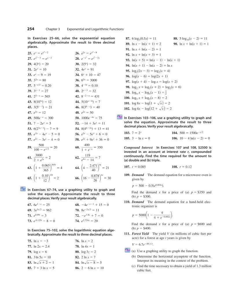
In Exercises 25–66, solve the exponential equation
algebraically. Approximate the result to three decimal
places.
25. 26.
27. 28.
29. 30.
31. 32.
33. 34.
35. 36.
37. 38.
39. 40.
41. 42.
43. 44.
45. 46.
47. 48.
49. 50.
51. 52.
53. 54.
55. 56.
57. 58.
59. 60.
61. 62.
63. 64.
65. 66.
In Exercises 67–74, use a graphing utility to graph and
solve the equation. Approximate the result to three
decimal places. Verify your result algebraically.
67. 68.
69. 70.
71. 72.
73. 74.
In Exercises 75–102, solve the logarithmic equation alge-
braically. Approximate the result to three decimal places.
75. 76.
77. 78.
79. 80.
81. 82.
83. 84.
85. 86.
87. 88.
89. 90.
91.
92.
93.
94.
95.
96.
97.
98.
99.
100.
101.
102.
In Exercises 103–106, use a graphing utility to graph and
solve the equation. Approximate the result to three
decimal places. Verify your result algebraically.
103. 104.
105. 106.
Compound Interest In Exercises 107 and 108, $2500 is
invested in an account at interest rate compounded
continuously. Find the time required for the amount to
(a) double and (b) triple.
107. 108.
109. Demand The demand equation for a microwave oven is
given by
Find the demand for a price of (a) and
(b)
110. Demand The demand equation for a hand-held elec-
tronic organizer is
Find the demand for a price of (a) and
(b)
111. Forest Yield The yield (in millions of cubic feet per
acre) for a forest at age years is given by
(a) Use a graphing utility to graph the function.
(b) Determine the horizontal asymptote of the function.
Interpret its meaning in the context of the problem.
(c) Find the time necessary to obtain a yield of 1.3 million
cubic feet.
V 5 6.7e248.1yt.
t
V
p 5 $400.
p 5 $600x
p 5 500011 24
4 1 e20.002x2.
p 5 $300.
p 5 $350x
p 5 500 2 0.5se0.004xd.
r 5 0.12r 5 0.085
r,
10 2 4 lnsx 2 2d 5 03 2 ln x 5 0
500 5 1500e2xy27 5 2x
log 4x 2 logs12 1 !x d 5 2
log 8x 2 logs1 1 !x d 5 2
log3 x 1 log3sx 2 8d 5 2
log4 x 2 log4sx 2 1d 512
log2 x 1 log2sx 1 2d 5 log2sx 1 6dlogsx 1 4d 2 log x 5 logsx 1 2dlogsx 2 6d 5 logs2x 1 1dlog2s2x 2 3d 5 log2sx 1 4dlnsx 1 1d 2 lnsx 2 2d 5 ln x
lnsx 1 5d 5 lnsx 2 1d 2 lnsx 1 1dln x 1 lnsx 1 3d 5 1
ln x 1 lnsx 2 2d 5 1
ln x 1 lnsx 1 1d 5 1ln x 2 lnsx 1 1d 5 2
5 log10sx 2 2d 5 116 log3s0.5xd 5 11
2 2 6 ln x 5 107 1 3 ln x 5 5
ln!x 2 8 5 5ln!x 1 2 5 1
2 ln x 5 73ln 5x 5 10
log 3z 5 2log x 5 6
ln 4x 5 1ln 2x 5 2.4
ln x 5 2ln x 5 23
e2.724x 5 29e 0.125t 2 8 5 0
2e1.8x 1 7 5 0e0.09t 5 3
8e22xy3 5 113e3xy2 5 962
24e2x21 1 15 5 06e12x 5 25
116 20.878
26 23t
5 3011 10.10
12 212t
5 2
14 22.471
40 29t
5 2111 10.065
365 2365t
5 4
119
e6x 2 145 7
3000
2 1 e2x5 2
400
1 1 e2x5 350
500
100 2 ex/25 20
e2x 1 9ex 1 36 5 0e2x 2 3ex 2 4 5 0
e2x 2 5ex 1 6 5 0e2x 2 4ex 2 5 5 0
8s4622xd 1 13 5 416s23x21d 2 7 5 9
214 1 3ex 5 117 2 2ex 5 5
1000e24x 5 75500e2x 5 300
e2x 5 50e3x 5 12
8s362xd 5 403s5x21d 5 21
5s10 x26d 5 78s103xd 5 12
8222x 5 431232x 5 565
2x23 5 323x21 5 27
423t 5 0.1052ty2 5 0.20
65x 5 300032x 5 80
6x 1 10 5 47ex 2 9 5 19
4ex 5 912ex 5 10
2s5xd 5 324s3xd 5 20
e2x25 ex2
22xex223 5 ex22
e2x 5 ex228ex 5 ex2
22
254 Chapter 3 Exponential and Logarithmic Functions

Section 3.4 Exponential and Logarithmic Equations 255
112. Trees per Acre The number of trees of a given
species per acre is approximated by the model
where is the average
diameter of the trees (in inches) 3 feet above the ground.
Use the model to approximate the average diameter of the
trees in a test plot when
113. Medicine The number of hospitals in the United
States from 1995 to 2002 can be modeled by
where represents the year, with corresponding to
1995. During which year did the number of hospitals
reach 5800? (Source: Health Forum)
114. Sports The number of daily fee golf facilities in the
United States from 1995 to 2003 can be modeled by
where represents
the year, with corresponding to 1995. During which
year did the number of daily fee golf facilities reach
9000? (Source: National Golf Foundation)
115. Average Heights The percent of American males
between the ages of 18 and 24 who are no more than
inches tall is modeled by
and the percent of American females between the ages of
18 and 24 who are no more than inches tall is modeled
by
(Source: U.S. National Center for Health Statistics)
(a) Use the graph to determine any horizontal asymptotes
of the graphs of the functions. Interpret the meaning
in the context of the problem.
(b) What is the average height of each sex?
116. Learning Curve In a group project in learning theory, a
mathematical model for the proportion of correct
responses after trials was found to be
(a) Use a graphing utility to graph the function.
(b) Use the graph to determine any horizontal asymptotes
of the graph of the function. Interpret the meaning of
the upper asymptote in the context of this problem.
(c) After how many trials will 60% of the responses be
correct?
P 50.83
1 1 e20.2n.
n
P
Height (in inches)
Per
cen
t o
f
po
pu
lati
on
x
f(x)
m(x)20
40
60
80
100
55 60 65 70 75
f sxd 5100
1 1 e20.66607sx264.51d.
x
f
msxd 5100
1 1 e20.6114sx269.71d
x
m
t 5 5
t5 ≤ t ≤ 13y 5 4381 1 1883.6 ln t,
y
t 5 5t
y 5 7312 2 630.0 ln t, 5 ≤ t ≤ 12
y
N 5 21.
x5 ≤ x ≤ 40N 5 68s1020.04xd,
N
x 0.2 0.4 0.6 0.8 1.0
y
117. Automobiles Automobiles are designed with crum-
ple zones that help protect their occupants in crashes.
The crumple zones allow the occupants to move short
distances when the automobiles come to abrupt stops.
The greater the distance moved, the fewer g’s the crash
victims experience. (One g is equal to the acceleration
due to gravity. For very short periods of time, humans
have withstood as much as 40 g’s.) In crash tests with
vehicles moving at 90 kilometers per hour, analysts
measured the numbers of g’s experienced during
deceleration by crash dummies that were permitted to
move meters during impact. The data are shown in
the table.
A model for the data is given by
where is the number of g’s.
(a) Complete the table using the model.
(b) Use a graphing utility to graph the data points and
the model in the same viewing window. How do
they compare?
(c) Use the model to estimate the distance traveled
during impact if the passenger deceleration must
not exceed 30 g’s.
(d) Do you think it is practical to lower the number of
g’s experienced during impact to fewer than 23?
Explain your reasoning.
y
y 5 23.00 1 11.88 ln x 136.94
x
x
Model It
x g’s
0.2 158
0.4 80
0.6 53
0.8 40
1.0 32
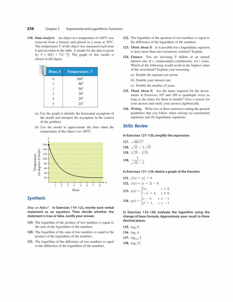
118. Data Analysis An object at a temperature of 160 C was
removed from a furnace and placed in a room at 20 C.
The temperature of the object was measured each hour
and recorded in the table. A model for the data is given
by The graph of this model is
shown in the figure.
(a) Use the graph to identify the horizontal asymptote of
the model and interpret the asymptote in the context
of the problem.
(b) Use the model to approximate the time when the
temperature of the object was 100 C.
Synthesis
True or False? In Exercises 119–122, rewrite each verbal
statement as an equation. Then decide whether the
statement is true or false. Justify your answer.
119. The logarithm of the product of two numbers is equal to
the sum of the logarithms of the numbers.
120. The logarithm of the sum of two numbers is equal to the
product of the logarithms of the numbers.
121. The logarithm of the difference of two numbers is equal
to the difference of the logarithms of the numbers.
122. The logarithm of the quotient of two numbers is equal to
the difference of the logarithms of the numbers.
123. Think About It Is it possible for a logarithmic equation
to have more than one extraneous solution? Explain.
124. Finance You are investing dollars at an annual
interest rate of compounded continuously, for years.
Which of the following would result in the highest value
of the investment? Explain your reasoning.
(a) Double the amount you invest.
(b) Double your interest rate.
(c) Double the number of years.
125. Think About It Are the times required for the invest-
ments in Exercises 107 and 108 to quadruple twice as
long as the times for them to double? Give a reason for
your answer and verify your answer algebraically.
126. Writing Write two or three sentences stating the general
guidelines that you follow when solving (a) exponential
equations and (b) logarithmic equations.
Skills Review
In Exercises 127–130, simplify the expression.
127.
128.
129.
130.
In Exercises 131–134, sketch a graph of the function.
131.
132.
133.
134.
In Exercises 135–138, evaluate the logarithm using the
change-of-base formula. Approximate your result to three
decimal places.
135.
136.
137.
138. log8 22
log3y4 5
log3 4
log6 9
gsxd 5 5x 2 3,
x2 1 1,
x ≤ 21
x > 21
gsxd 5 52x,
2x2 1 4,
x < 0
x ≥ 0
f sxd 5 |x 1 2| 2 8
f sxd 5 |x| 1 9
3
!10 2 2
3!25 ? 3!15
!32 2 2!25
!48x2y 5
tr,
P
T
h
Tem
per
atu
re
(in
deg
rees
Cel
siu
s)
20
40
60
80
100
120
140
160
1 2 3 4 5 6 7 8
Hour
8
T 5 20 f1 1 7s22hdg.h
T
8
8
256 Chapter 3 Exponential and Logarithmic Functions
Hour, h Temperature, T
0
1
2
3
4
5 248
298
388
568
908
1608
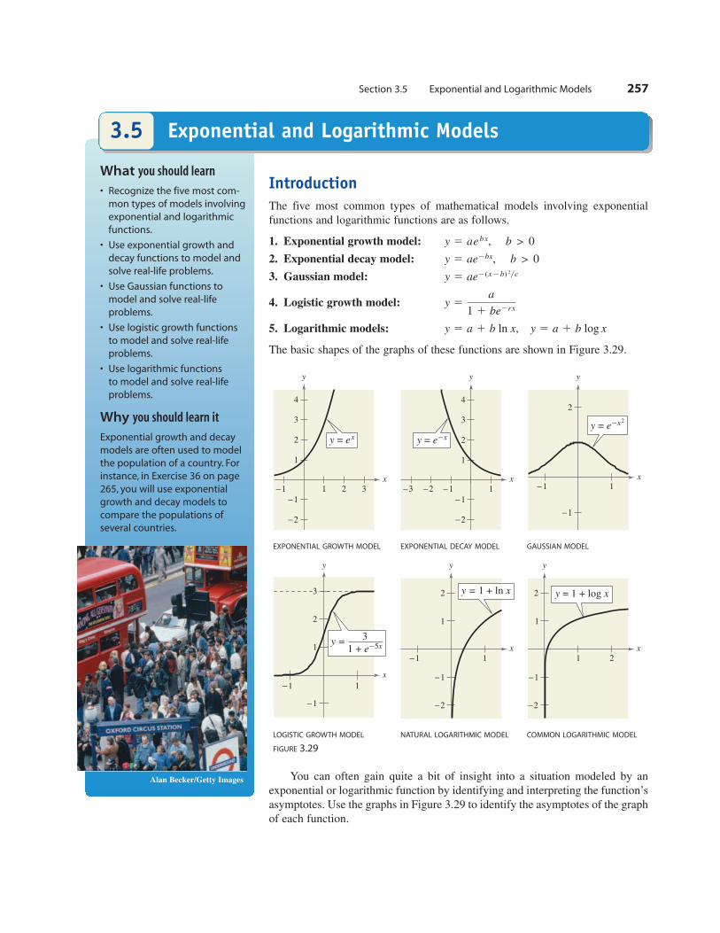
Section 3.5 Exponential and Logarithmic Models 257
Introduction
The five most common types of mathematical models involving exponential
functions and logarithmic functions are as follows.
1. Exponential growth model:
2. Exponential decay model:
3. Gaussian model:
4. Logistic growth model:
5. Logarithmic models:
The basic shapes of the graphs of these functions are shown in Figure 3.29.
EXPONENTIAL GROWTH MODEL EXPONENTIAL DECAY MODEL GAUSSIAN MODEL
LOGISTIC GROWTH MODEL NATURAL LOGARITHMIC MODEL COMMON LOGARITHMIC MODEL
FIGURE 3.29
You can often gain quite a bit of insight into a situation modeled by an
exponential or logarithmic function by identifying and interpreting the function’s
asymptotes. Use the graphs in Figure 3.29 to identify the asymptotes of the graph
of each function.
x
1 2
−1
−2
2
1
y = 1 + log x
y
x
−1 1
−1
−2
2
1
y = 1 + ln x
y
x
y
−1 1
−1
1
2
3
y = 3
1 + e−5x
x−1 1
−1
2
y
y = e−x2
x
−1 1−2−3
−1
−2
1
2
3
4
y
y = e−x
x
−1 21 3
−1
−2
1
2
3
4
y
y = ex
y 5 a 1 b ln x, y 5 a 1 b log x
y 5a
1 1 be2rx
y 5 ae2(x2b)2yc
y 5 ae2bx, b > 0
y 5 aebx, b > 0
What you should learn
• Recognize the five most com-
mon types of models involving
exponential and logarithmic
functions.
• Use exponential growth and
decay functions to model and
solve real-life problems.
• Use Gaussian functions to
model and solve real-life
problems.
• Use logistic growth functions
to model and solve real-life
problems.
• Use logarithmic functions
to model and solve real-life
problems.
Why you should learn it
Exponential growth and decay
models are often used to model
the population of a country. For
instance, in Exercise 36 on page
265, you will use exponential
growth and decay models to
compare the populations of
several countries.
Exponential and Logarithmic Models
Alan Becker/Getty Images
3.5
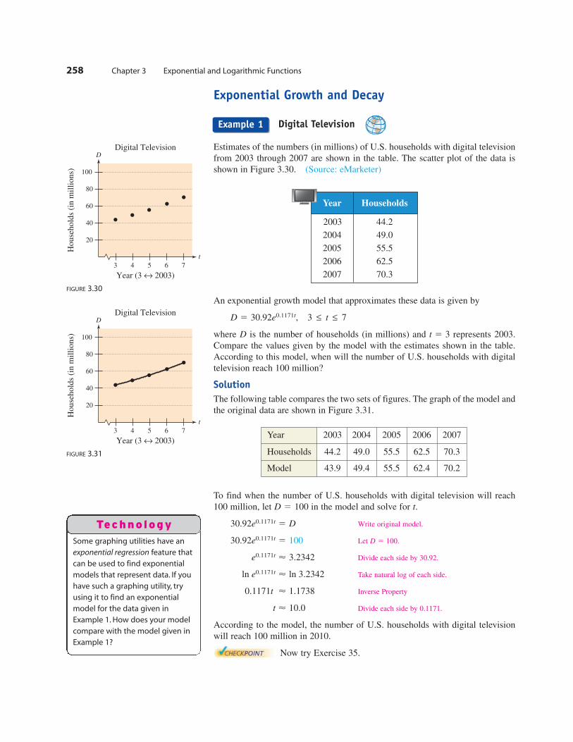
Exponential Growth and Decay
Digital Television
Estimates of the numbers (in millions) of U.S. households with digital television
from 2003 through 2007 are shown in the table. The scatter plot of the data is
shown in Figure 3.30. (Source: eMarketer)
An exponential growth model that approximates these data is given by
where is the number of households (in millions) and represents 2003.
Compare the values given by the model with the estimates shown in the table.
According to this model, when will the number of U.S. households with digital
television reach 100 million?
Solution
The following table compares the two sets of figures. The graph of the model and
the original data are shown in Figure 3.31.
To find when the number of U.S. households with digital television will reach
100 million, let in the model and solve for
Write original model.
Let
Divide each side by 30.92.
Take natural log of each side.
Inverse Property
Divide each side by 0.1171.
According to the model, the number of U.S. households with digital television
will reach 100 million in 2010.
Now try Exercise 35.
t < 10.0
0.1171t < 1.1738
ln e0.1171t < ln 3.2342
e0.1171t < 3.2342
D 5 100. 30.92e0.1171t 5 100
30.92e0.1171t 5 D
t.D 5 100
t 5 3D
D 5 30.92e0.1171t, 3 ≤ t ≤ 7
258 Chapter 3 Exponential and Logarithmic Functions
Example 1
t
D
Year (3 ↔ 2003)
Digital Television
House
hold
s (i
n m
illi
ons)
3 4 5 6 7
20
40
60
80
100
FIGURE 3.30
t
D
Year (3 ↔ 2003)
Digital Television
House
hold
s (i
n m
illi
ons)
3 4 5 6 7
20
40
60
80
100
FIGURE 3.31
Year Households
2003 44.2
2004 49.0
2005 55.5
2006 62.5
2007 70.3
Year 2003 2004 2005 2006 2007
Households 44.2 49.0 55.5 62.5 70.3
Model 43.9 49.4 55.5 62.4 70.2
Some graphing utilities have an
exponential regression feature that
can be used to find exponential
models that represent data. If you
have such a graphing utility, try
using it to find an exponential
model for the data given in
Example 1. How does your model
compare with the model given in
Example 1?
Techno logy
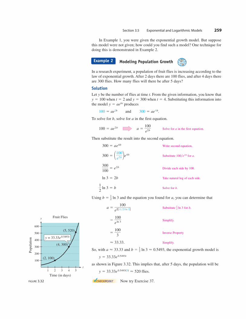
In Example 1, you were given the exponential growth model. But suppose
this model were not given; how could you find such a model? One technique for
doing this is demonstrated in Example 2.
Modeling Population Growth
In a research experiment, a population of fruit flies is increasing according to the
law of exponential growth. After 2 days there are 100 flies, and after 4 days there
are 300 flies. How many flies will there be after 5 days?
Solution
Let be the number of flies at time From the given information, you know that
when and when . Substituting this information into
the model produces
and
To solve for solve for in the first equation.
Solve for a in the first equation.
Then substitute the result into the second equation.
Write second equation.
Substitute 100 for a.
Divide each side by 100.
Take natural log of each side.
Solve for b.
Using and the equation you found for you can determine that
Substitute for b.
Simplify.
Inverse Property
Simplify.
So, with and the exponential growth model is
as shown in Figure 3.32. This implies that, after 5 days, the population will be
Now try Exercise 37.
y 5 33.33e0.5493s5d < 520 flies.
y 5 33.33e0.5493t
b 512 ln 3 < 0.5493,a < 33.33
< 33.33.
5100
3
5100
e ln 3
12 ln 3 a 5
100
e2fs1y2d ln 3g
a,b 512 ln 3
1
2 ln 3 5 b
ln 3 5 2b
300
1005 e2b
ye2b 300 5 1100
e2b 2e4b
300 5 ae4b
a 5100
e2b100 5 ae2b
ab,
300 5 ae4b.100 5 ae2b
y 5 aebt
t 5 4y 5 300t 5 2y 5 100
t.y
Section 3.5 Exponential and Logarithmic Models 259
Time (in days)
Popula
tion
y
t
(2, 100)
(4, 300)
(5, 520)
y = 33.33e0.5493t
Fruit Flies
1 2 3 4 5
100
200
300
400
500
600
FIGURE 3.32
Example 2
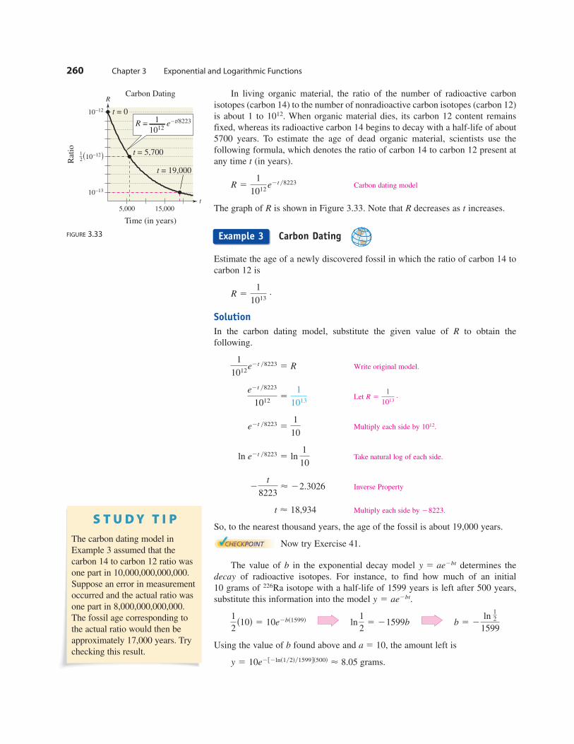
In living organic material, the ratio of the number of radioactive carbon
isotopes (carbon 14) to the number of nonradioactive carbon isotopes (carbon 12)
is about 1 to When organic material dies, its carbon 12 content remains
fixed, whereas its radioactive carbon 14 begins to decay with a half-life of about
5700 years. To estimate the age of dead organic material, scientists use the
following formula, which denotes the ratio of carbon 14 to carbon 12 present at
any time (in years).
Carbon dating model
The graph of is shown in Figure 3.33. Note that decreases as increases.
Carbon Dating
Estimate the age of a newly discovered fossil in which the ratio of carbon 14 to
carbon 12 is
Solution
In the carbon dating model, substitute the given value of to obtain the
following.
Write original model.
Let
Multiply each side by
Take natural log of each side.
Inverse Property
Multiply each side by 8223.
So, to the nearest thousand years, the age of the fossil is about 19,000 years.
Now try Exercise 41.
The value of in the exponential decay model determines the
decay of radioactive isotopes. For instance, to find how much of an initial
10 grams of isotope with a half-life of 1599 years is left after 500 years,
substitute this information into the model
Using the value of found above and 10, the amount left is
y 5 10e2f2lns1y2dy1599gs500d < 8.05 grams.
a 5b
b 5 2ln
12
1599ln
1
25 21599b
1
2s10d 5 10e2bs1599d
y 5 ae2bt.
226Ra
y 5 ae2btb
2 t < 18,934
2t
8223< 22.3026
ln e2t y8223 5 ln 1
10
1012. e2t y8223 51
10
R 51
1013 .
e2t y8223
10125
1
1013
1
1012e2t y8223 5 R
R
R 51
1013.
tRR
R 51
1012e2t y8223
t
1012.
260 Chapter 3 Exponential and Logarithmic Functions
5,000 15,000
R
t
Time (in years)
10−13
10−12
10−12( )12R
atio t = 5,700
Carbon Dating
t = 0
t = 19,000
R = e−t/8223 1012
1
FIGURE 3.33 Example 3
The carbon dating model in
Example 3 assumed that the
carbon 14 to carbon 12 ratio was
one part in 10,000,000,000,000.
Suppose an error in measurement
occurred and the actual ratio was
one part in 8,000,000,000,000.
The fossil age corresponding to
the actual ratio would then be
approximately 17,000 years. Try
checking this result.
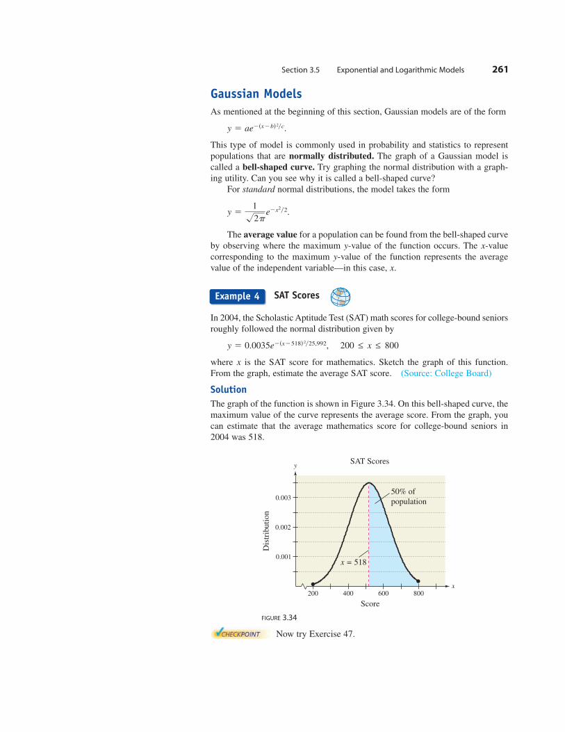
Gaussian Models
As mentioned at the beginning of this section, Gaussian models are of the form
This type of model is commonly used in probability and statistics to represent
populations that are normally distributed. The graph of a Gaussian model is
called a bell-shaped curve. Try graphing the normal distribution with a graph-
ing utility. Can you see why it is called a bell-shaped curve?
For standard normal distributions, the model takes the form
The average value for a population can be found from the bell-shaped curve
by observing where the maximum value of the function occurs. The -value
corresponding to the maximum value of the function represents the average
value of the independent variable—in this case,
SAT Scores
In 2004, the Scholastic Aptitude Test (SAT) math scores for college-bound seniors
roughly followed the normal distribution given by
where is the SAT score for mathematics. Sketch the graph of this function.
From the graph, estimate the average SAT score. (Source: College Board)
Solution
The graph of the function is shown in Figure 3.34. On this bell-shaped curve, the
maximum value of the curve represents the average score. From the graph, you
can estimate that the average mathematics score for college-bound seniors in
2004 was 518.
FIGURE 3.34
Now try Exercise 47.
Dis
trib
uti
on
Score
200 400 600 800
0.001
0.003
x
y
x = 518
0.002
SAT Scores
50% of
population
x
y 5 0.0035e2sx2518d2y25,992, 200 ≤ x ≤ 800
x.
y-
xy-
y 51
!2pe2x2y2.
y 5 ae2sx2bd2yc.
Section 3.5 Exponential and Logarithmic Models 261
Example 4

Logistic Growth Models
Some populations initially have rapid growth, followed by a declining rate of
growth, as indicated by the graph in Figure 3.35. One model for describing this
type of growth pattern is the logistic curve given by the function
where is the population size and is the time. An example is a bacteria culture
that is initially allowed to grow under ideal conditions, and then under less
favorable conditions that inhibit growth. A logistic growth curve is also called a
sigmoidal curve.
Spread of a Virus
On a college campus of 5000 students, one student returns from vacation with a
contagious and long-lasting flu virus. The spread of the virus is modeled by
where is the total number of students infected after days. The college will
cancel classes when 40% or more of the students are infected.
a. How many students are infected after 5 days?
b. After how many days will the college cancel classes?
Solution
a. After 5 days, the number of students infected is
b. Classes are canceled when the number infected is
So, after about 10 days, at least 40% of the students will be infected, and the
college will cancel classes. The graph of the function is shown in Figure 3.36.
Now try Exercise 49.
t < 10.1
t 5 21
0.8 ln
1.5
4999
20.8t 5 ln 1.5
4999
ln e20.8t 5 ln 1.5
4999
e20.8t 51.5
4999
1 1 4999e20.8t 5 2.5
2000 55000
1 1 4999e20.8t
s0.40ds5000d 5 2000.
< 54.55000
1 1 4999e24y 5
5000
1 1 4999e20.8s5d
ty
y 55000
1 1 4999e20.8t, t ≥ 0
xy
y 5a
1 1 be2r x
262 Chapter 3 Exponential and Logarithmic Functions
Example 5
Stu
den
ts i
nfe
cted
Time (in days)
2 4 6 8 10
500
1000
1500
2000
2500
y
(10.1, 2000)
(5, 54)t
12 14
Flu Virus
FIGURE 3.36
x
Decreasing
rate of
growth
Increasing
rate of
growth
y
FIGURE 3.35
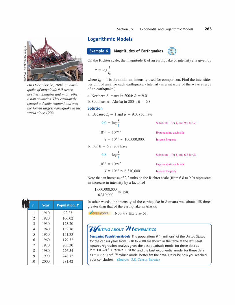
Logarithmic Models
Magnitudes of Earthquakes
On the Richter scale, the magnitude of an earthquake of intensity is given by
where is the minimum intensity used for comparison. Find the intensities
per unit of area for each earthquake. (Intensity is a measure of the wave energy
of an earthquake.)
a. Northern Sumatra in 2004:
b. Southeastern Alaska in 2004:
Solution
a. Because and you have
Substitute 1 for and 9.0 for
Exponentiate each side.
Inverse Property
b. For you have
Substitute 1 for and 6.8 for
Exponentiate each side.
Inverse Property
Note that an increase of 2.2 units on the Richter scale (from 6.8 to 9.0) represents
an increase in intensity by a factor of
In other words, the intensity of the earthquake in Sumatra was about 158 times
greater than that of the earthquake in Alaska.
Now try Exercise 51.
1,000,000,000
6,310,000< 158.
I 5 106.8 < 6,310,000.
106.8 5 10log I
R.I0 6.8 5 log
I
1
R 5 6.8,
I 5 109.0 < 100,000,000.
109.0 5 10log I
R.I0 9.0 5 log I
1
R 5 9.0,I0 5 1
R 5 6.8
R 5 9.0
I0 5 1
R 5 logI
I0
IR
Section 3.5 Exponential and Logarithmic Models 263
Example 6
W RITING ABOUT MATHEMATICS
Comparing Population Models The populations P (in millions) of the United States
for the census years from 1910 to 2000 are shown in the table at the left. Least
squares regression analysis gives the best quadratic model for these data as
and the best exponential model for these data
as Which model better fits the data? Describe how you reached
your conclusion. (Source: U.S. Census Bureau)
P 5 82.677e0.124t.
P 5 1.0328t 2 1 9.607t 1 81.82,
On December 26, 2004, an earth-
quake of magnitude 9.0 struck
northern Sumatra and many other
Asian countries. This earthquake
caused a deadly tsunami and was
the fourth largest earthquake in the
world since 1900.
BA
Y IS
MO
YO
/AF
P/G
ett
y Im
ag
es
t Year Population, P
1 1910 92.23
2 1920 106.02
3 1930 123.20
4 1940 132.16
5 1950 151.33
6 1960 179.32
7 1970 203.30
8 1980 226.54
9 1990 248.72
10 2000 281.42
264 Chapter 3 Exponential and Logarithmic Functions
Exercises 3.5
In Exercises 1–6, match the function with its graph. [The
graphs are labeled (a), (b), (c), (d), (e), and (f ).]
(a) (b)
(c) (d)
(e) (f )
1. 2.
3. 4.
5. 6.
Compound Interest In Exercises 7–14, complete the table
for a savings account in which interest is compounded
continuously.
Initial Annual Time to Amount After
Investment % Rate Double 10 Years
7. $1000 3.5%
8. $750
9. $750
10. $10,000 12 yr
11. $500 $1505.00
12. $600 $19,205.00
13. 4.5% $10,000.00
14. 2% $2000.00
Compound Interest In Exercises 15 and 16, determine the
principal that must be invested at rate compounded
monthly, so that $500,000 will be available for retirement
in years.
15. 16.
Compound Interest In Exercises 17 and 18, determine the
time necessary for $1000 to double if it is invested at
interest rate compounded (a) annually, (b) monthly,
(c) daily, and (d) continuously.
17. 18.
19. Compound Interest Complete the table for the time
necessary for dollars to triple if interest is compounded
continuously at rate
20. Modeling Data Draw a scatter plot of the data in
Exercise 19. Use the regression feature of a graphing
utility to find a model for the data.
r.
P
t
r 5 1012%r 5 11%
r
r 5 12%, t 5 40r 5 712%, t 5 20
t
r,P
jj
jj
jj
jj
jj
j734 yrj
jj1012%
jj
y 54
1 1 e22xy 5 lnsx 1 1d
y 5 3e2sx22d2y5y 5 6 1 logsx 1 2d
y 5 6e2xy4y 5 2e xy4
−2
4
x2 4
6
2
−2
y
−6−12 6 12
6
x
y
x
y
−2 2 4 6
2
4
−4−8 4 8
8
12
4
x
y
x2 4 6
2
4
8
y
−4
x2 4 6
2
4
6
−2
y
VOCABULARY CHECK: Fill in the blanks.
1. An exponential growth model has the form ________ and an exponential decay model has the form ________.
2. A logarithmic model has the form ________ or ________.
3. Gaussian models are commonly used in probability and statistics to represent populations that are ________ ________.
4. The graph of a Gaussian model is ________ shaped, where the ________ ________ is the maximum -value of the graph.
5. A logistic curve is also called a ________ curve.
PREREQUISITE SKILLS REVIEW: Practice and review algebra skills needed for this section at www.Eduspace.com.
y
r 2% 4% 6% 8% 10% 12%
t
Section 3.5 Exponential and Logarithmic Models 265
21. Compound Interest Complete the table for the time
necessary for dollars to triple if interest is compounded
annually at rate
22. Modeling Data Draw a scatter plot of the data in
Exercise 21. Use the regression feature of a graphing utili-
ty to find a model for the data.
23. Comparing Models If $1 is invested in an account over a
10-year period, the amount in the account, where repre-
sents the time in years, is given by or
depending on whether the account pays simple
interest at or continuous compound interest at 7%.
Graph each function on the same set of axes. Which grows
at a higher rate? (Remember that is the greatest integer
function discussed in Section 1.6.)
24. Comparing Models If $1 is invested in an account over a
10-year period, the amount in the account, where repre-
sents the time in years, is given by
or
depending on whether the account pays simple interest at
6% or compound interest at compounded daily. Use a
graphing utility to graph each function in the same viewing
window. Which grows at a higher rate?
Radioactive Decay In Exercises 25–30, complete the table
for the radioactive isotope.
Half-life Initial Amount After
Isotope (years) Quantity 1000 Years
25. 1599 10 g
26. 1599 1.5 g
27. 5715 2 g
28. 5715 3 g
29. 24,100 2.1 g
30. 24,100 0.4 g
In Exercises 31–34, find the exponential model
that fits the points shown in the graph or table.
31. 32.
33. 34.
35. Population The population (in thousands) of
Pittsburgh, Pennsylvania from 2000 through 2003 can be
modeled by where represents the year,
with corresponding to 2000. (Source: U.S. Census
Bureau)
(a) According to the model, was the population of
Pittsburgh increasing or decreasing from 2000 to 2003?
Explain your reasoning.
(b) What were the populations of Pittsburgh in 2000 and
2003?
(c) According to the model, when will the population be
approximately 2.3 million?
t 5 0
tP 5 2430e20.0029t,
P
x
1 2 3 4
2
4
6
8
(4, 5)
( )12
0,
y
x
1 2 3 4 5
2
4
6
8
10 (3, 10)
(0, 1)
y
y 5 aebx
j239Pu
j239Pu
j14C
j14C
j226Ra
j226Ra
512%
A 5 11 10.055
365 2v365tb
A 5 1 1 0.06 v t b
t
vtb
712%
A 5 e0.07t
A 5 1 1 0.075v t bt
r.
P
t
r 2% 4% 6% 8% 10% 12%
t
x 0 4
y 5 1
x 0 3
y 1 14
36. Population The table shows the populations (in
millions) of five countries in 2000 and the projected
populations (in millions) for the year 2010. (Source:
U.S. Census Bureau)
(a) Find the exponential growth or decay model
or for the population of each
country by letting correspond to 2000. Use
the model to predict the population of each country
in 2030.
(b) You can see that the populations of the United
States and the United Kingdom are growing at
different rates. What constant in the equation
is determined by these different growth
rates? Discuss the relationship between the different
growth rates and the magnitude of the constant.
(c) You can see that the population of China is
increasing while the population of Bulgaria is
decreasing. What constant in the equation
reflects this difference? Explain.
y 5 aebt
y 5 aebt
t 5 0
y 5 ae2bty 5 aebt
Model It
Country 2000 2010
Bulgaria 7.8 7.1
Canada 31.3 34.3
China 1268.9 1347.6
United Kingdom 59.5 61.2
United States 282.3 309.2
37. Website Growth The number of hits a new search-
engine website receives each month can be modeled by
where represents the number of months the website has
been operating. In the website’s third month, there were
10,000 hits. Find the value of and use this result to
predict the number of hits the website will receive after
24 months.
38. Value of a Painting The value (in millions of dollars)
of a famous painting can be modeled by
where represents the year, with corresponding to
1990. In 2004, the same painting was sold for $65 million.
Find the value of and use this result to predict the value
of the painting in 2010.
39. Bacteria Growth The number of bacteria in a culture
is modeled by
where is the time in hours. If when esti-
mate the time required for the population to double in size.
40. Bacteria Growth The number of bacteria in a culture
is modeled by
where is the time in hours. If when
estimate the time required for the population to double in
size.
41. Carbon Dating
(a) The ratio of carbon 14 to carbon 12 in a piece of wood
discovered in a cave is Estimate the age of
the piece of wood.
(b) The ratio of carbon 14 to carbon 12 in a piece of paper
buried in a tomb is Estimate the age of the
piece of paper.
42. Radioactive Decay Carbon 14 dating assumes that the
carbon dioxide on Earth today has the same radioactive
content as it did centuries ago. If this is true, the amount of
absorbed by a tree that grew several centuries ago
should be the same as the amount of absorbed by a tree
growing today. A piece of ancient charcoal contains only
15% as much radioactive carbon as a piece of modern
charcoal. How long ago was the tree burned to make the
ancient charcoal if the half-life of is 5715 years?
43. Depreciation A 2005 Jeep Wrangler that costs $30,788
new has a book value of $18,000 after 2 years.
(a) Find the linear model
(b) Find the exponential model
(c) Use a graphing utility to graph the two models in the
same viewing window. Which model depreciates faster
in the first 2 years?
(d) Find the book values of the vehicle after 1 year and
after 3 years using each model.
(e) Explain the advantages and disadvantages of using
each model to a buyer and a seller.
44. Depreciation A Dell Inspiron 8600 laptop computer that
costs $1150 new has a book value of $550 after 2 years.
(a) Find the linear model
(b) Find the exponential model
(c) Use a graphing utility to graph the two models in the
same viewing window. Which model depreciates faster
in the first 2 years?
(d) Find the book values of the computer after 1 year and
after 3 years using each model.
(e) Explain the advantages and disadvantages to a buyer
and a seller of using each model.
45. Sales The sales (in thousands of units) of a new CD
burner after it has been on the market for years are
modeled by
Fifteen thousand units of the new product were sold the
first year.
(a) Complete the model by solving for
(b) Sketch the graph of the model.
(c) Use the model to estimate the number of units sold
after 5 years.
46. Learning Curve The management at a plastics factory
has found that the maximum number of units a worker can
produce in a day is 30. The learning curve for the number
of units produced per day after a new employee has
worked days is modeled by
After 20 days on the job, a new employee produces 19
units.
(a) Find the learning curve for this employee (first, find the
value of ).
(b) How many days should pass before this employee is
producing 25 units per day?
47. IQ Scores The IQ scores from a sample of a class of
returning adult students at a small northeastern college
roughly follow the normal distribution
where is the IQ score.
(a) Use a graphing utility to graph the function.
(b) From the graph in part (a), estimate the average IQ
score of an adult student.
x
70 ≤ x ≤ 115y 5 0.0266e2sx2100d2y450,
k
N 5 30s1 2 ekt d.
t
N
k.
Sstd 5 100s1 2 ektd.
t
S
V 5 aekt.
V 5 mt 1 b.
V 5 aekt.
V 5 mt 1 b.
14C
14C
14C
R 5 1y1311.
R 5 1y814.
t 5 10,N 5 280t
N 5 250ekt
N
t 5 5,N 5 300t
N 5 100ekt
N
k,
t 5 0t
V 5 10ekt
V
k,
t
y 5 4080ekt
y
266 Chapter 3 Exponential and Logarithmic Functions
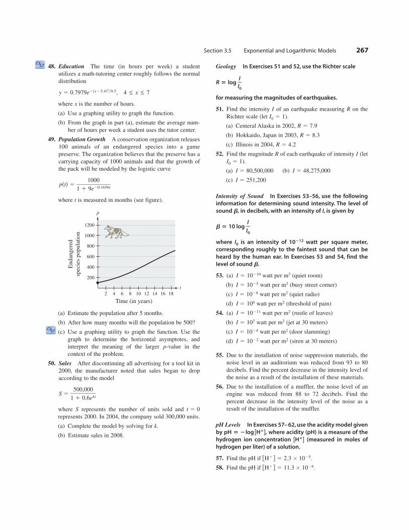
Section 3.5 Exponential and Logarithmic Models 267
48. Education The time (in hours per week) a student
utilizes a math-tutoring center roughly follows the normal
distribution
where is the number of hours.
(a) Use a graphing utility to graph the function.
(b) From the graph in part (a), estimate the average num-
ber of hours per week a student uses the tutor center.
49. Population Growth A conservation organization releases
100 animals of an endangered species into a game
preserve. The organization believes that the preserve has a
carrying capacity of 1000 animals and that the growth of
the pack will be modeled by the logistic curve
where is measured in months (see figure).
(a) Estimate the population after 5 months.
(b) After how many months will the population be 500?
(c) Use a graphing utility to graph the function. Use the
graph to determine the horizontal asymptotes, and
interpret the meaning of the larger -value in the
context of the problem.
50. Sales After discontinuing all advertising for a tool kit in
2000, the manufacturer noted that sales began to drop
according to the model
where represents the number of units sold and
represents 2000. In 2004, the company sold 300,000 units.
(a) Complete the model by solving for
(b) Estimate sales in 2008.
Geology In Exercises 51 and 52, use the Richter scale
for measuring the magnitudes of earthquakes.
51. Find the intensity of an earthquake measuring on the
Richter scale (let ).
(a) Centeral Alaska in 2002,
(b) Hokkaido, Japan in 2003,
(c) Illinois in 2004,
52. Find the magnitude of each earthquake of intensity (let
).
(a) (b)
(c)
Intensity of Sound In Exercises 53–56, use the following
information for determining sound intensity. The level of
sound in decibels, with an intensity of , is given by
where is an intensity of watt per square meter,
corresponding roughly to the faintest sound that can be
heard by the human ear. In Exercises 53 and 54, find the
level of sound
53. (a) watt per (quiet room)
(b) watt per (busy street corner)
(c) watt per (quiet radio)
(d) watt per (threshold of pain)
54. (a) watt per (rustle of leaves)
(b) watt per (jet at 30 meters)
(c) watt per (door slamming)
(d) watt per (siren at 30 meters)
55. Due to the installation of noise suppression materials, the
noise level in an auditorium was reduced from 93 to 80
decibels. Find the percent decrease in the intensity level of
the noise as a result of the installation of these materials.
56. Due to the installation of a muffler, the noise level of an
engine was reduced from 88 to 72 decibels. Find the
percent decrease in the intensity level of the noise as a
result of the installation of the muffler.
pH Levels In Exercises 57– 62, use the acidity model given
by where acidity (pH) is a measure of the
hydrogen ion concentration (measured in moles of
hydrogen per liter) of a solution.
57. Find the pH if
58. Find the pH if fH1g 5 11.3 3 1026.
fH1g 5 2.3 3 1025.
[H1]
pH 5 2log [H1],
m2I 5 1022
m2I 5 1024
m2I 5 102
m2I 5 10211
m2I 5 100
m2I 5 1028
m2I 5 1025
m2I 5 10210
b.
10212I0
b 5 10 log I
I0
Ib,
I 5 251,200
I 5 48,275,000I 5 80,500,000
I0 5 1
IR
R 5 4.2
R 5 8.3
R 5 7.9
I0 5 1
RI
R 5 log I
I0
k.
t 5 0S
S 5500,000
1 1 0.6ekt
p
Time (in years)
En
dan
ger
ed
spec
ies
po
pu
lati
on
2 4 6 8 10 12 14 16 18
200
400
600
800
1000
1200
t
p
t
pstd 51000
1 1 9e20.1656t
x
4 ≤ x ≤ 7y 5 0.7979e2sx25.4d2y0.5,
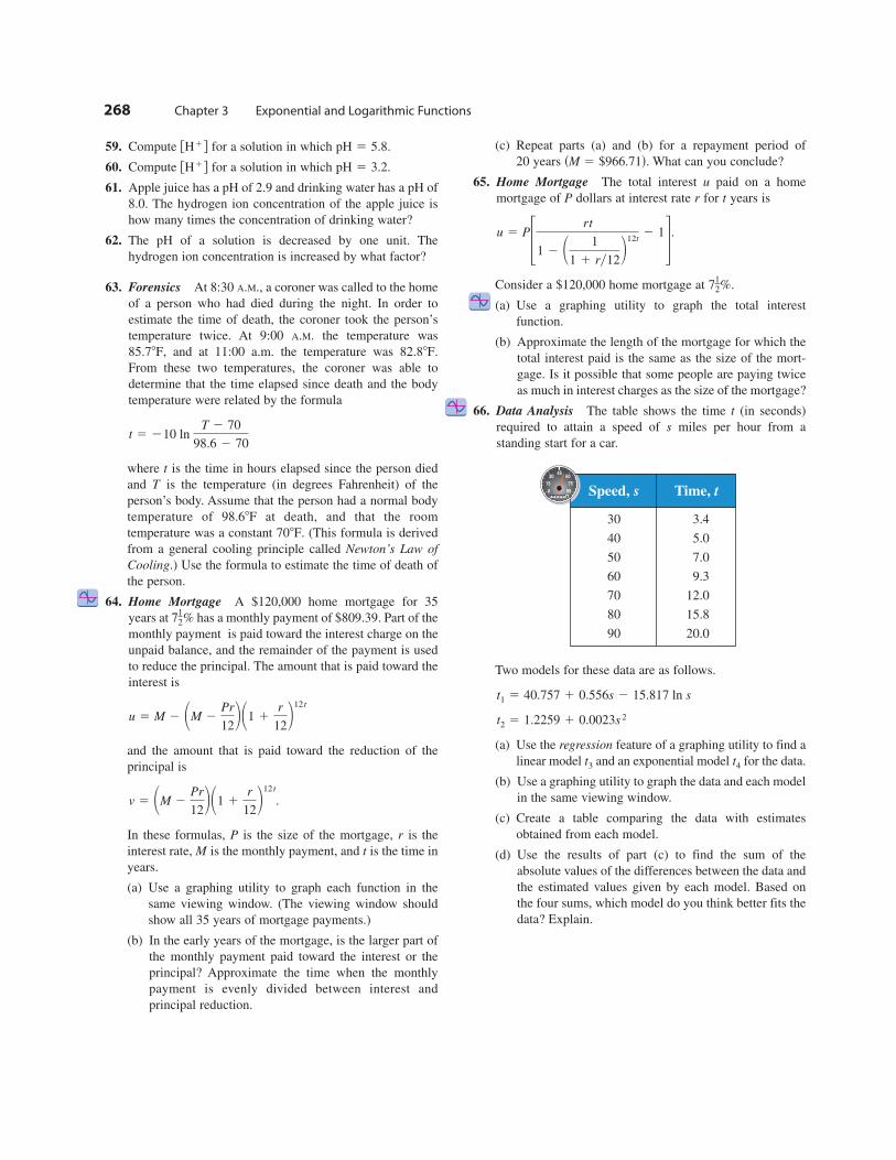
59. Compute for a solution in which pH 5.8.
60. Compute for a solution in which pH 3.2.
61. Apple juice has a pH of 2.9 and drinking water has a pH of
8.0. The hydrogen ion concentration of the apple juice is
how many times the concentration of drinking water?
62. The pH of a solution is decreased by one unit. The
hydrogen ion concentration is increased by what factor?
63. Forensics At 8:30 A.M., a coroner was called to the home
of a person who had died during the night. In order to
estimate the time of death, the coroner took the person’s
temperature twice. At 9:00 A.M. the temperature was
and at 11:00 a.m. the temperature was
From these two temperatures, the coroner was able to
determine that the time elapsed since death and the body
temperature were related by the formula
where is the time in hours elapsed since the person died
and is the temperature (in degrees Fahrenheit) of the
person’s body. Assume that the person had a normal body
temperature of at death, and that the room
temperature was a constant (This formula is derived
from a general cooling principle called Newton’s Law of
Cooling.) Use the formula to estimate the time of death of
the person.
64. Home Mortgage A $120,000 home mortgage for 35
years at has a monthly payment of $809.39. Part of the
monthly payment is paid toward the interest charge on the
unpaid balance, and the remainder of the payment is used
to reduce the principal. The amount that is paid toward the
interest is
and the amount that is paid toward the reduction of the
principal is
In these formulas, is the size of the mortgage, is the
interest rate, is the monthly payment, and is the time in
years.
(a) Use a graphing utility to graph each function in the
same viewing window. (The viewing window should
show all 35 years of mortgage payments.)
(b) In the early years of the mortgage, is the larger part of
the monthly payment paid toward the interest or the
principal? Approximate the time when the monthly
payment is evenly divided between interest and
principal reduction.
(c) Repeat parts (a) and (b) for a repayment period of
20 years What can you conclude?
65. Home Mortgage The total interest paid on a home
mortgage of dollars at interest rate for years is
Consider a $120,000 home mortgage at
(a) Use a graphing utility to graph the total interest
function.
(b) Approximate the length of the mortgage for which the
total interest paid is the same as the size of the mort-
gage. Is it possible that some people are paying twice
as much in interest charges as the size of the mortgage?
66. Data Analysis The table shows the time (in seconds)
required to attain a speed of miles per hour from a
standing start for a car.
Two models for these data are as follows.
(a) Use the regression feature of a graphing utility to find a
linear model and an exponential model for the data.
(b) Use a graphing utility to graph the data and each model
in the same viewing window.
(c) Create a table comparing the data with estimates
obtained from each model.
(d) Use the results of part (c) to find the sum of the
absolute values of the differences between the data and
the estimated values given by each model. Based on
the four sums, which model do you think better fits the
data? Explain.
t4t3
t2 5 1.2259 1 0.0023s 2
t1 5 40.757 1 0.556s 2 15.817 ln s
s
t
712%.
u 5 P3rt
1 2 1 1
1 1 ry12212t
2 14.
trP
u
sM 5 $966.71d.
tM
rP
v 5 1M 2Pr
12211 1r
12212t
.
u 5 M 2 1M 2Pr
12211 1r
12212t
712%
708F.
98.68F
T
t
t 5 210 ln T 2 70
98.6 2 70
82.88F.85.78F,
5fH1g5fH1g
268 Chapter 3 Exponential and Logarithmic Functions
Speed, s Time, t
30 3.4
40 5.0
50 7.0
60 9.3
70 12.0
80 15.8
90 20.0
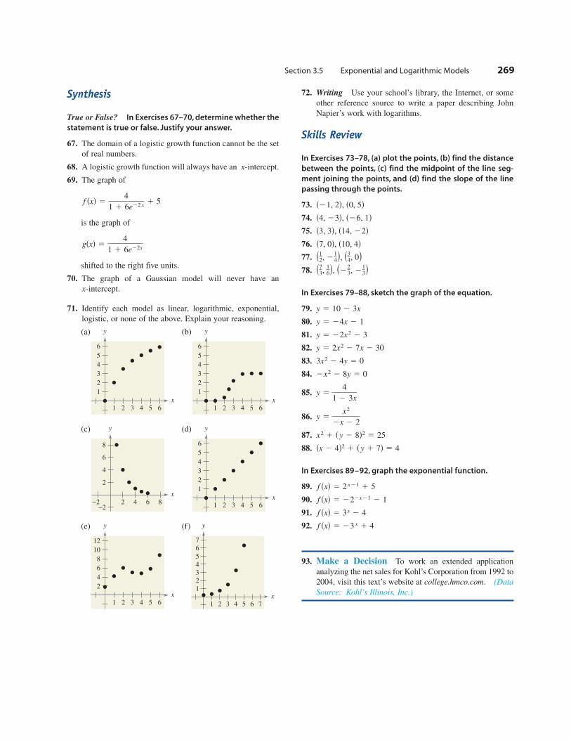
Section 3.5 Exponential and Logarithmic Models 269
Synthesis
True or False? In Exercises 67–70, determine whether the
statement is true or false. Justify your answer.
67. The domain of a logistic growth function cannot be the set
of real numbers.
68. A logistic growth function will always have an -intercept.
69. The graph of
is the graph of
shifted to the right five units.
70. The graph of a Gaussian model will never have an
-intercept.
71. Identify each model as linear, logarithmic, exponential,
logistic, or none of the above. Explain your reasoning.
(a) (b)
(c) (d)
(e) (f)
72. Writing Use your school’s library, the Internet, or some
other reference source to write a paper describing John
Napier’s work with logarithms.
Skills Review
In Exercises 73–78, (a) plot the points, (b) find the distance
between the points, (c) find the midpoint of the line seg-
ment joining the points, and (d) find the slope of the line
passing through the points.
73.
74.
75.
76.
77.
78.
In Exercises 79–88, sketch the graph of the equation.
79.
80.
81.
82.
83.
84.
85.
86.
87.
88.
In Exercises 89–92, graph the exponential function.
89.
90.
91.
92.
93. Make a Decision To work an extended application
analyzing the net sales for Kohl’s Corporation from 1992 to
2004, visit this text’s website at college.hmco.com. (Data
Source: Kohl’s Illinois, Inc.)
f sxd 5 23 x 1 4
f sxd 5 3x 2 4
f sxd 5 222x21 2 1
f sxd 5 2 x21 1 5
sx 2 4d2 1 sy 1 7d 5 4
x2 1 sy 2 8d2 5 25
y 5x2
2x 2 2
y 54
1 2 3x
2x2 2 8y 5 0
3x2 2 4y 5 0
y 5 2x2 2 7x 2 30
y 5 22x2 2 3
y 5 24x 2 1
y 5 10 2 3x
s73,
16d, s22
3, 213d
s12, 2
14d, s3
4, 0ds7, 0d, s10, 4ds3, 3d, s14, 22ds4, 23d, s26, 1ds21, 2d, s0, 5d
1 2 3 4 5 6 7
1234567
x
y
1 2 3 4 5 6
2
4
6
8
10
12
x
y
1 2 3 4 5 6
1
2
3
4
5
6
x
y
2−2 4 6 8
2
−2
4
6
8
x
y
1 2 3 4 5 6
1
2
3
4
5
6
x
y
1 2 3 4 5 6
1
2
3
4
5
6
x
y
x
gsxd 54
1 1 6e22x
f sxd 54
1 1 6e22 x1 5
x

270 Chapter 3 Exponential and Logarithmic Functions
Chapter Summary3
What did you learn?
Section 3.1 Review Exercisesh Recognize and evaluate exponential functions with base a (p. 218). 1–6
h Graph exponential functions and use the One-to-One Property (p. 219). 7–26
h Recognize, evaluate, and graph exponential functions with base e (p. 222). 27–34
h Use exponential functions to model and solve real-life problems (p. 223). 35–40
Section 3.2h Recognize and evaluate logarithmic functions with base a (p. 229). 41–52
h Graph logarithmic functions (p. 231). 53–58
h Recognize, evaluate, and graph natural logarithmic functions (p. 233). 59–68
h Use logarithmic functions to model and solve real-life problems (p. 235). 69, 70
Section 3.3h Use the change-of-base formula to rewrite and evaluate logarithmic expressions (p. 239). 71–74
h Use properties of logarithms to evaluate or rewrite logarithmic expressions (p. 240). 75–78
h Use properties of logarithms to expand or condense logarithmic expressions (p. 241). 79–94
h Use logarithmic functions to model and solve real-life problems (p. 242). 95, 96
Section 3.4h Solve simple exponential and logarithmic equations (p. 246). 97–104
h Solve more complicated exponential equations (p. 247). 105–118
h Solve more complicated logarithmic equations (p. 249). 119–134
h Use exponential and logarithmic equations to model and solve 135, 136
real-life problems (p. 251).
Section 3.5h Recognize the five most common types of models involving exponential 137–142
and logarithmic functions (p. 257).
h Use exponential growth and decay functions to model and solve 143–148
real-life problems (p. 258).
h Use Gaussian functions to model and solve real-life problems (p. 261). 149
h Use logistic growth functions to model and solve real-life problems (p. 262). 150
h Use logarithmic functions to model and solve real-life problems (p. 263). 151, 152
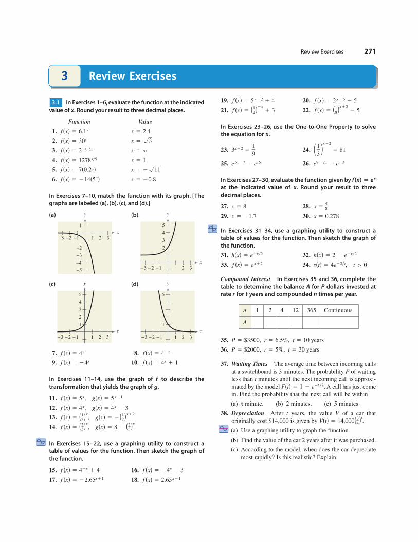
Review Exercises 271
In Exercises 1–6, evaluate the function at the indicated
value of Round your result to three decimal places.
Function Value
1.
2.
3.
4.
5.
6.
In Exercises 7–10, match the function with its graph. [The
graphs are labeled (a), (b), (c), and (d).]
(a) (b)
(c) (d)
7. 8.
9. 10.
In Exercises 11–14, use the graph of to describe the
transformation that yields the graph of
11.
12.
13.
14.
In Exercises 15–22, use a graphing utility to construct a
table of values for the function. Then sketch the graph of
the function.
15. 16.
17. 18.
19. 20.
21. 22.
In Exercises 23–26, use the One-to-One Property to solve
the equation for
23. 24.
25. 26.
In Exercises 27–30, evaluate the function given by
at the indicated value of Round your result to three
decimal places.
27. 28.
29. 30.
In Exercises 31–34, use a graphing utility to construct a
table of values for the function. Then sketch the graph of
the function.
31. 32.
33. 34.
Compound Interest In Exercises 35 and 36, complete the
table to determine the balance for dollars invested at
rate for years and compounded times per year.
35.
36.
37. Waiting Times The average time between incoming calls
at a switchboard is 3 minutes. The probability of waiting
less than minutes until the next incoming call is approxi-
mated by the model A call has just come
in. Find the probability that the next call will be within
(a) minute. (b) 2 minutes. (c) 5 minutes.
38. Depreciation After years, the value of a car that
originally cost $14,000 is given by
(a) Use a graphing utility to graph the function.
(b) Find the value of the car 2 years after it was purchased.
(c) According to the model, when does the car depreciate
most rapidly? Is this realistic? Explain.
Vstd 5 14,000s34dt
.
Vt
12
Fstd 5 1 2 e2t y3.
t
F
P 5 $2000, r 5 5%, t 5 30 years
P 5 $3500, r 5 6.5%, t 5 10 years
ntr
PA
t > 0sstd 5 4e22yt,f sxd 5 e x12
hsxd 5 2 2 e2xy2hsxd 5 e2xy2
x 5 0.278x 5 21.7
x 558x 5 8
x.
f xxc 5 ex
e822x 5 e23e5x27 5 e15
11
32x22
5 813x12 51
9
x.
f sxd 5 s18dx12
2 5f sxd 5 s12d2x
1 3
f sxd 5 2 x26 2 5f sxd 5 5 x22 1 4
f sxd 5 2.65x21f sxd 5 22.65x11
f sxd 5 24x 2 3f sxd 5 42x 1 4
gsxd 5 8 2 s23dx
f sxd 5 s23dx
,
gsxd 5 2s12dx12
f sxd 5 s12dx
,
gsxd 5 4x 2 3f sxd 5 4x,
gsxd 5 5x21f sxd 5 5x,
g.
f
f sxd 5 4x 1 1f sxd 5 24x
f sxd 5 42xf sxd 5 4x
−3 −1−2 3x
21
1
5
y
3x
2
1
2
3
4
5
y
−3 −1−2 1
−3 −1−2 3x
2
2
3
4
5
y
−3 −1 1−2 3x
2
1
−2
−3
−4
−5
y
x 5 20.8 f sxd 5 214s5xdx 5 2!11 f sxd 5 7s0.2xdx 5 1 f sxd 5 1278xy5
x 5 p f sxd 5 220.5x
x 5 !3 f sxd 5 30x
x 5 2.4 f sxd 5 6.1x
x.
3.1
Review Exercises3
n 1 2 4 12 365 Continuous
A
39. Trust Fund On the day a person is born, a deposit of
$50,000 is made in a trust fund that pays 8.75% interest,
compounded continuously.
(a) Find the balance on the person’s 35th birthday.
(b) How much longer would the person have to wait for
the balance in the trust fund to double?
40. Radioactive Decay Let represent a mass of plutonium
241 (in grams), whose half-life is 14.4 years. The
quantity of plutonium 241 present after years is given by
(a) Determine the initial quantity (when ).
(b) Determine the quantity present after 10 years.
(c) Sketch the graph of this function over the interval
to
In Exercises 41– 44, write the exponential equation in
logarithmic form.
41. 42.
43. 44.
In Exercises 45– 48, evaluate the function at the indicated
value of without using a calculator.
Function Value
45.
46.
47.
48.
In Exercises 49–52, use the One-to-One Property to solve
the equation for
49. 50.
51. 52.
In Exercises 53–58, find the domain, -intercept, and vertical
asymptote of the logarithmic function and sketch its graph.
53. 54.
55. 56.
57. 58.
In Exercises 59–64, use a calculator to evaluate the function
given by at the indicated value of Round your
result to three decimal places if necessary.
59. 60.
61. 62.
63. 64.
In Exercises 65–68, find the domain, -intercept, and vertical
asymptote of the logarithmic function and sketch its graph.
65. 66.
67. 68.
69. Antler Spread The antler spread (in inches) and
shoulder height (in inches) of an adult male American elk
are related by the model
Approximate the shoulder height of a male American elk
with an antler spread of 55 inches.
70. Snow Removal The number of miles of roads cleared
of snow is approximated by the model
where is the depth of the snow in inches. Use this model
to find when inches.
In Exercises 71–74, evaluate the logarithm using the
change-of-base formula. Do each exercise twice, once with
common logarithms and once with natural logarithms.
Round your the results to three decimal places.
71. 72.
73. 74.
In Exercises 75–78, use the properties of logarithms to
rewrite and simplify the logarithmic expression.
75. 76.
77. 78.
In Exercises 79–86, use the properties of logarithms to
expand the expression as a sum, difference, and/or
constant multiple of logarithms. (Assume all variables are
positive.)
79. 80.
81. 82.
83. 84.
85. 86.
In Exercises 87–94, condense the expression to the
logarithm of a single quantity.
87. 88.
89. 90.
91. 92.
93.
94. 5 lns x 2 2d 2 lns x 1 2d 2 3 lnx
12 lns2x 2 1d 2 2 lns x 1 1d
22 log x 2 5 logsx 1 6d13 log8sx 1 4d 1 7 log8 y
3 ln x 1 2 lnsx 1 1dln x 214 ln y
log6 y 2 2 log6 zlog2 5 1 log2 x
y > 1ln1y 2 1
4 22
,ln1x 1 3
xy 2ln 3xy2ln x2y2z
log7 !x
4log3
63!x
log 7x4log5 5x 2
lns3e24dln 20
log2s 112dlog 18
log3 0.28log1y2 5
log12 200log4 9
3.3
h 5 10s
h
2 ≤ h ≤ 15s 5 25 213 lnshy12d
ln 3,
s
h 5 116 logsa 1 40d 2 176.
h
a
f sxd 514 ln xhsxd 5 lnsx2d
f sxd 5 lnsx 2 3df sxd 5 ln x 1 3
x
x 5!3
8x 5 !7 1 5
x 5 e7x 5 e212
x 5 0.98x 5 22.6
x.f xxc 5 ln x
f sxd 5 logsx 2 3d 1 1 f sxd 5 4 2 logsx 1 5d
f sxd 5 6 1 log x f sxd 5 log1x
32gsxd 5 log5 xgsxd 5 log7 x
x
lns2x 2 1d 5 ln 11lnsx 1 9d 5 ln 4
log8s3x 2 10d 5 log8 5log4sx 1 7d 5 log4 14
x.
x 514f sxd 5 log4 x
x 518gsxd 5 log2 x
x 5 3gsxd 5 log9 x
x 5 1000f sxd 5 log x
x
e05 1e0.8
5 2.2255 . . .
253y25 12543
5 64
3.2
t 5 100.
t 5 0
t 5 0
Q 5 100s12dty14.4
.
t
s241PudQ
272 Chapter 3 Exponential and Logarithmic Functions
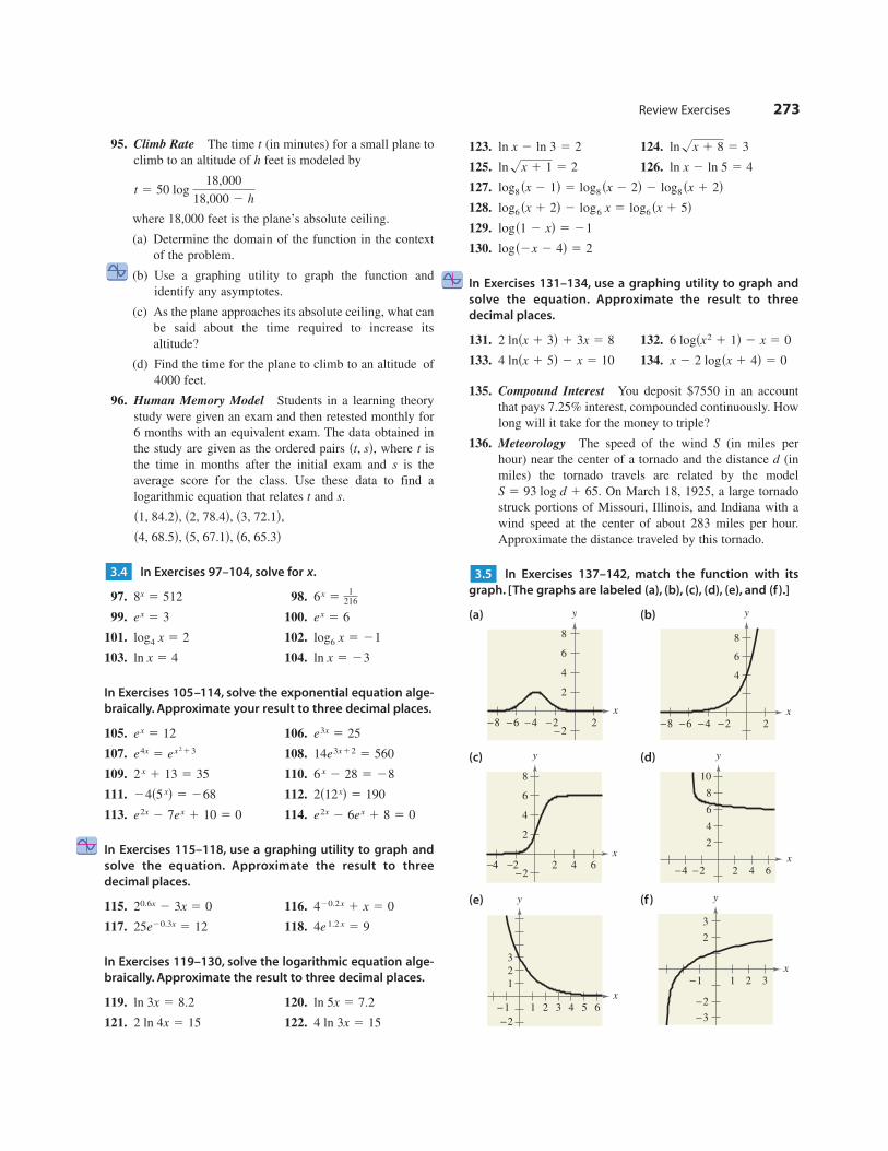
Review Exercises 273
95. Climb Rate The time (in minutes) for a small plane to
climb to an altitude of feet is modeled by
where 18,000 feet is the plane’s absolute ceiling.
(a) Determine the domain of the function in the context
of the problem.
(b) Use a graphing utility to graph the function and
identify any asymptotes.
(c) As the plane approaches its absolute ceiling, what can
be said about the time required to increase its
altitude?
(d) Find the time for the plane to climb to an altitude of
4000 feet.
96. Human Memory Model Students in a learning theory
study were given an exam and then retested monthly for
6 months with an equivalent exam. The data obtained in
the study are given as the ordered pairs where is
the time in months after the initial exam and is the
average score for the class. Use these data to find a
logarithmic equation that relates and
In Exercises 97–104, solve for
97. 98.
99. 100.
101. 102.
103. 104.
In Exercises 105–114, solve the exponential equation alge-
braically. Approximate your result to three decimal places.
105. 106.
107. 108.
109. 110.
111. 112.
113. 114.
In Exercises 115–118, use a graphing utility to graph and
solve the equation. Approximate the result to three
decimal places.
115. 116.
117. 118.
In Exercises 119–130, solve the logarithmic equation alge-
braically. Approximate the result to three decimal places.
119. 120.
121. 122.
123. 124.
125. 126.
127.
128.
129.
130.
In Exercises 131–134, use a graphing utility to graph and
solve the equation. Approximate the result to three
decimal places.
131. 132.
133. 134.
135. Compound Interest You deposit $7550 in an account
that pays 7.25% interest, compounded continuously. How
long will it take for the money to triple?
136. Meteorology The speed of the wind (in miles per
hour) near the center of a tornado and the distance (in
miles) the tornado travels are related by the model
On March 18, 1925, a large tornado
struck portions of Missouri, Illinois, and Indiana with a
wind speed at the center of about 283 miles per hour.
Approximate the distance traveled by this tornado.
In Exercises 137–142, match the function with its
graph. [The graphs are labeled (a), (b), (c), (d), (e), and (f).]
(a) (b)
(c) (d)
(e) (f )
−1
x
3
2
3
1 2
−2
−3
y
−1
x
3
2
1
6
3
1 2 4
−2
5
y
−2−4
x
2
8
4
6
2
6
10
4
y
−2−4
x
2
8
4
6
2
4 6−2
y
−8 −2−4
x
2
8
4
−6
6
y
−8 −2−4
x
2
2
6
4
−6
8
−2
y
3.5
S 5 93 log d 1 65.
d
S
x 2 2 logsx 1 4d 5 04 lnsx 1 5d 2 x 5 10
6 logsx2 1 1d 2 x 5 02 lnsx 1 3d 1 3x 5 8
logs2x 2 4d 5 2
logs1 2 xd 5 21
log6 sx 1 2d 2 log6 x 5 log6 sx 1 5dlog8 sx 2 1d 5 log8 sx 2 2d 2 log8 sx 1 2d
ln x 2 ln 5 5 4ln!x 1 1 5 2
ln!x 1 8 5 3ln x 2 ln 3 5 2
4 ln 3x 5 152 ln 4x 5 15
ln 5x 5 7.2ln 3x 5 8.2
4e 1.2 x 5 925e20.3x 5 12
420.2x 1 x 5 020.6x 2 3x 5 0
e2x 2 6ex 1 8 5 0e2x 2 7ex 1 10 5 0
2s12xd 5 19024s5 xd 5 268
6 x 2 28 5 282 x 1 13 5 35
14e3x12 5 560e4x 5 ex213
e3x 5 25ex 5 12
ln x 5 23ln x 5 4
log6 x 5 21log4 x 5 2
ex 5 6ex 5 3
6x 51
2168x 5 512
x.3.4
s4, 68.5d, s5, 67.1d, s6, 65.3ds1, 84.2d, s2, 78.4d, s3, 72.1d,
s.t
s
tst, sd,
t 5 50 log 18,000
18,000 2 h
h
t
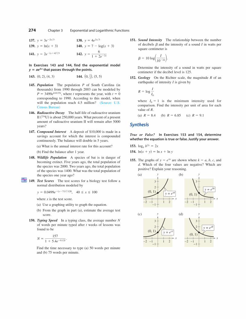
137. 138.
139. 140.
141. 142.
In Exercises 143 and 144, find the exponential model
that passes through the points.
143. 144.
145. Population The population of South Carolina (in
thousands) from 1990 through 2003 can be modeled by
where represents the year, with
corresponding to 1990. According to this model, when
will the population reach 4.5 million? (Source: U.S.
Census Bureau)
146. Radioactive Decay The half-life of radioactive uranium
II is about 250,000 years. What percent of a present
amount of radioactive uranium II will remain after 5000
years?
147. Compound Interest A deposit of $10,000 is made in a
savings account for which the interest is compounded
continuously. The balance will double in 5 years.
(a) What is the annual interest rate for this account?
(b) Find the balance after 1 year.
148. Wildlife Population A species of bat is in danger of
becoming extinct. Five years ago, the total population of
the species was 2000. Two years ago, the total population
of the species was 1400. What was the total population of
the species one year ago?
149. Test Scores The test scores for a biology test follow a
normal distribution modeled by
where is the test score.
(a) Use a graphing utility to graph the equation.
(b) From the graph in part (a), estimate the average test
score.
150. Typing Speed In a typing class, the average number
of words per minute typed after weeks of lessons was
found to be
Find the time necessary to type (a) 50 words per minute
and (b) 75 words per minute.
151. Sound Intensity The relationship between the number
of decibels and the intensity of a sound in watts per
square centimeter is
Determine the intensity of a sound in watts per square
centimeter if the decibel level is 125.
152. Geology On the Richter scale, the magnitude of an
earthquake of intensity is given by
where is the minimum intensity used for
comparison. Find the intensity per unit of area for each
value of
(a) (b) (c)
Synthesis
True or False? In Exercises 153 and 154, determine
whether the equation is true or false. Justify your answer.
153.
154.
155. The graphs of are shown where and
Which of the four values are negative? Which are
positive? Explain your reasoning.
(a) (b)
(c) (d)
x
−2 −1 21−1
2
3
(0, 1)
y = edt
y
x
−2 −1 21−1
2
3
(0, 1) y = ect
y
x
−2 −1 21−1
3
(0, 1)
y = ebt
y
x
−2 −1 21−1
2
3
(0, 1)y = eat
y
d.
c,b,k 5 a,y 5 e kt
lnsx 1 yd 5 ln x 1 ln y
logb b2x 5 2x
R 5 9.1R 5 6.85R 5 8.4
R.
I0 5 1
R 5 log I
I0
I
R
b 5 10 log1 I
102162.
Ib
N 5157
1 1 5.4e20.12t .
t
N
x
40 ≤ x ≤ 100y 5 0.0499e2sx271d2y128,
s234Ud
t 5 0tP 5 3499e0.0135t,
P
s5, 5ds0, 12d,s4, 3ds0, 2d,
y 5 aebx
y 56
1 1 2e22xy 5 2e2sx14d2y3
y 5 7 2 logsx 1 3dy 5 lnsx 1 3dy 5 4e2xy3y 5 3e22xy3
274 Chapter 3 Exponential and Logarithmic Functions
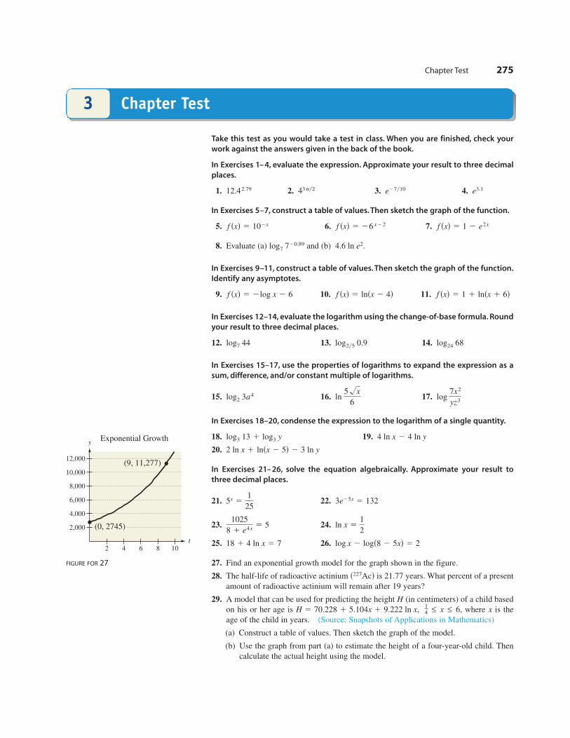
Chapter Test 275
Chapter Test3
Take this test as you would take a test in class. When you are finished, check your
work against the answers given in the back of the book.
In Exercises 1– 4, evaluate the expression. Approximate your result to three decimal
places.
1. 2. 3. 4.
In Exercises 5–7, construct a table of values. Then sketch the graph of the function.
5. 6. 7.
8. Evaluate (a) and (b)
In Exercises 9–11, construct a table of values. Then sketch the graph of the function.
Identify any asymptotes.
9. 10. 11.
In Exercises 12–14, evaluate the logarithm using the change-of-base formula. Round
your result to three decimal places.
12. 13. 14.
In Exercises 15–17, use the properties of logarithms to expand the expression as a
sum, difference, and/or constant multiple of logarithms.
15. 16. 17.
In Exercises 18–20, condense the expression to the logarithm of a single quantity.
18. 19.
20.
In Exercises 21– 26, solve the equation algebraically. Approximate your result to
three decimal places.
21. 22.
23. 24.
25. 26.
27. Find an exponential growth model for the graph shown in the figure.
28. The half-life of radioactive actinium is 21.77 years. What percent of a present
amount of radioactive actinium will remain after 19 years?
29. A model that can be used for predicting the height (in centimeters) of a child based
on his or her age is where is the
age of the child in years. (Source: Snapshots of Applications in Mathematics)
(a) Construct a table of values. Then sketch the graph of the model.
(b) Use the graph from part (a) to estimate the height of a four-year-old child. Then
calculate the actual height using the model.
x14 ≤ x ≤ 6,H 5 70.228 1 5.104x 1 9.222 ln x,
H
s227Acd
log x 2 logs8 2 5xd 5 218 1 4 ln x 5 7
ln x 51
2
1025
8 1 e4x5 5
3e25x 5 1325x 51
25
2 ln x 1 lnsx 2 5d 2 3 ln y
4 ln x 2 4 ln ylog3 13 1 log3 y
log 7x2
yz3ln
5!x
6log2 3a4
log24 68log2y5 0.9log7 44
f sxd 5 1 1 lnsx 1 6df sxd 5 lnsx 2 4df sxd 5 2log x 2 6
4.6 ln e2.log7 720.89
f sxd 5 1 2 e2xf sxd 5 26 x22f sxd 5 102x
e3.1e27y1043py212.42.79
2,000
4 6 8 10t
y
4,000
6,000
8,000
10,000
12,000
2
(9, 11,277)
Exponential Growth
(0, 2745)
FIGURE FOR 27
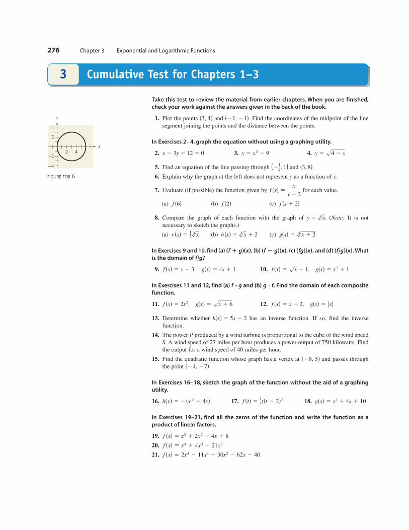
276 Chapter 3 Exponential and Logarithmic Functions
Cumulative Test for Chapters 1–33
Take this test to review the material from earlier chapters. When you are finished,
check your work against the answers given in the back of the book.
1. Plot the points and Find the coordinates of the midpoint of the line
segment joining the points and the distance between the points.
In Exercises 2– 4, graph the equation without using a graphing utility.
2. 3. 4.
5. Find an equation of the line passing through and
6. Explain why the graph at the left does not represent as a function of
7. Evaluate (if possible) the function given by for each value.
(a) (b) (c)
8. Compare the graph of each function with the graph of (Note: It is not
necessary to sketch the graphs.)
(a) (b) (c)
In Exercises 9 and 10, find (a) (b) (c) and (d) What
is the domain of
9. 10.
In Exercises 11 and 12, find (a) and (b) Find the domain of each composite
function.
11. 12.
13. Determine whether has an inverse function. If so, find the inverse
function.
14. The power produced by a wind turbine is proportional to the cube of the wind speed
A wind speed of 27 miles per hour produces a power output of 750 kilowatts. Find
the output for a wind speed of 40 miles per hour.
15. Find the quadratic function whose graph has a vertex at and passes through
the point
In Exercises 16–18, sketch the graph of the function without the aid of a graphing
utility.
16. 17. 18.
In Exercises 19–21, find all the zeros of the function and write the function as a
product of linear factors.
19.
20.
21. f sxd 5 2x4 2 11x3 1 30x2 2 62x 2 40
f sxd 5 x4 1 4x3 2 21x2
f sxd 5 x3 1 2x2 1 4x 1 8
gssd 5 s2 1 4s 1 10f std 514tst 2 2d2hsxd 5 2sx 2 1 4xd
s24, 27d.s28, 5d
S.
P
hsxd 5 5x 2 2
gsxd 5 |x|f sxd 5 x 2 2,gsxd 5 !x 1 6f sxd 5 2x2,
g 8 f.f 8 g
gsxd 5 x2 1 1f sxd 5 !x 2 1,gsxd 5 4x 1 1f sxd 5 x 2 3,
f/g?
xf/gcxxc.xfgcxxc,xf 2 gcxxc,xf 1 gcxxc,
gsxd 5 3!x 1 2hsxd 5 3!x 1 2r sxd 512
3!x
y 5 3!x.
f ss 1 2df s2df s6d
f sxd 5x
x 2 2
x.y
s3, 8d.s212, 1d
y 5 !4 2 xy 5 x2 2 9x 2 3y 1 12 5 0
s21, 21d.s3, 4d
2
2
4
−2
−4
4x
y
FIGURE FOR 6
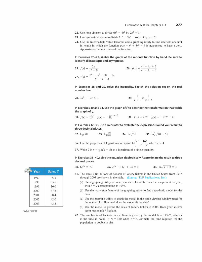
Cumulative Test for Chapters 1–3 277
22. Use long division to divide by
23. Use synthetic division to divide by
24. Use the Intermediate Value Theorem and a graphing utility to find intervals one unit
in length in which the function is guaranteed to have a zero.
Approximate the real zeros of the function.
In Exercises 25–27, sketch the graph of the rational function by hand. Be sure to
identify all intercepts and asymptotes.
25. 26.
27.
In Exercises 28 and 29, solve the inequality. Sketch the solution set on the real
number line.
28. 29.
In Exercises 30 and 31, use the graph of to describe the transformation that yields
the graph of
30. 31.
In Exercises 32–35, use a calculator to evaluate the expression. Round your result to
three decimal places.
32. 33. 34. 35.
36. Use the properties of logarithms to expand where
37. Write as a logarithm of a single quantity.
In Exercises 38–40, solve the equation algebraicially. Approximate the result to three
decimal places.
38. 39. 40.
41. The sales (in billions of dollars) of lottery tickets in the United States from 1997
through 2003 are shown in the table. (Source: TLF Publications, Inc.)
(a) Use a graphing utility to create a scatter plot of the data. Let represent the year,
with corresponding to 1997.
(b) Use the regression feature of the graphing utility to find a quadratic model for the
data.
(c) Use the graphing utility to graph the model in the same viewing window used for
the scatter plot. How well does the model fit the data?
(d) Use the model to predict the sales of lottery tickets in 2008. Does your answer
seem reasonable? Explain.
42. The number of bacteria in a culture is given by the model where
is the time in hours. If when estimate the time required for the
population to double in size.
t 5 8,N 5 420
tN 5 175ekt,N
t 5 7
t
S
ln!x 1 2 5 3e2x 2 11ex 1 24 5 06e2x 5 72
2 ln x 212 lnsx 1 5d
x > 4.ln1x2 2 16
x 4 2,
lns!40 2 5dln!31logs67dlog 98
gsxd 5 22.2x 1 4f sxd 5 2.2x,gsxd 5 2s25d2x13
f sxd 5 s25dx
,
g.
f
1
x 1 1≥
1
x 1 53x3 2 12x ≤ 0
f sxd 5x3 1 3x2 2 4x 2 12
x2 2 x 2 2
f sxd 5x2 2 4x 1 3
x2 2 2x 2 3 f sxd 5
2x
x2 2 9
gsxd 5 x3 1 3x2 2 6
x 1 2.2x 4 1 3x3 2 6x 1 5
2x2 1 1.6x3 2 4x2
Year Sales, S
1997 35.5
1998 35.6
1999 36.0
2000 37.2
2001 38.4
2002 42.0
2003 43.5
TABLE FOR 41
Each of the following three properties of logarithms can be proved by using prop-
erties of exponential functions.
Proof
Let
and
The corresponding exponential forms of these two equations are
and
To prove the Product Property, multiply u and v to obtain
The corresponding logarithmic form of is So,
To prove the Quotient Property, divide u by v to obtain
The corresponding logarithmic form of is So,
To prove the Power Property, substitute for u in the expression as
follows.
Substitute for
Property of exponents
Inverse Property of Logarithms
Substitute for
So, loga un 5 n loga u.
x.loga u 5 n loga u
5 nx
5 loga anx
u.ax loga un 5 logasa
xdn
loga un,ax
loga u
v5 loga u 2 loga v.
logasuyvd 5 x 2 y.uyv 5 ax2y
u
v5
ax
ay5 a x2y.
loga v.logasuvd 5 loga u 1
logasuvd 5 x 1 y.uv 5 ax1y
uv 5 axay 5 ax1y.
ay 5 v.ax 5 u
y 5 loga v.x 5 loga u
278
Proofs in Mathematics
Slide Rules
The slide rule was invented by
William Oughtred (1574–1660)
in 1625. The slide rule is a
computational device with a
sliding portion and a fixed
portion. A slide rule enables
you to perform multiplication
by using the Product Property
of Logarithms. There are other
slide rules that allow for the
calculation of roots and trigono-
metric functions. Slide rules
were used by mathematicians
and engineers until the invention
of the hand-held calculator in
1972.
Properties of Logarithms (p. 240)
Let be a positive number such that and let be a real number. If
and are positive real numbers, the following properties are true.
Logarithm with Base a Natural Logarithm
1. Product Property:
2. Quotient Property:
3. Power Property: ln un 5 n ln uloga un 5 n loga u
ln u
v5 ln u 2 ln vloga
u
v5 loga u 2 loga v
lnsuvd 5 ln u 1 ln vlogasuvd 5 loga u 1 loga v
v
una Þ 1,a

279
1. Graph the exponential function given by for
1.2, and 2.0. Which of these curves intersects the line
Determine all positive numbers for which the
curve intersects the line
2. Use a graphing utility to graph and each of the
functions and Which
function increases at the greatest rate as approaches
3. Use the result of Exercise 2 to make a conjecture about the
rate of growth of and where is a natural
number and approaches
4. Use the results of Exercises 2 and 3 to describe what is
implied when it is stated that a quantity is growing
exponentially.
5. Given the exponential function
show that
(a)
(b)
6. Given that
and
show that
7. Use a graphing utility to compare the graph of
the function given by with the graph of each given
function. (read “ factorial” is defined as
(a)
(b)
(c)
8. Identify the pattern of successive polynomials given in
Exercise 7. Extend the pattern one more term and compare
the graph of the resulting polynomial function with the
graph of What do you think this pattern implies?
9. Graph the function given by
From the graph, the function appears to be one-to-one.
Assuming that the function has an inverse function, find
10. Find a pattern for if
where
11. By observation, identify the equation that corresponds to
the graph. Explain your reasoning.
(a)
(b)
(c)
12. You have two options for investing $500. The first earns
7% compounded annually and the second earns 7% simple
interest. The figure shows the growth of each investment
over a 30-year period.
(a) Identify which graph represents each type of invest-
ment. Explain your reasoning.
(b) Verify your answer in part (a) by finding the equations
that model the investment growth and graphing the
models.
(c) Which option would you choose? Explain your
reasoning.
13. Two different samples of radioactive isotopes are decaying.
The isotopes have initial amounts of and as well as
half-lives of and respectively. Find the time required
for the samples to decay to equal amounts.
k2,k1
c2,c1
t
Year
Inves
tmen
t
(in d
oll
ars)
5 10 15 20 25 30
1000
2000
3000
4000
y 5 6s1 2 e2x2y2d
y 56
1 1 e2xy2
y 5 6e2x2y2
−2−4−2
42x
4
6
8
y
a Þ 1.a > 0,
f sxd 5ax 1 1
ax 2 1
f 21sxd
f 21sxd.
f sxd 5 e x 2 e2x.
y 5 ex.
y3 5 1 1x
1!1
x2
2!1
x3
3!
y2 5 1 1x
1!1
x2
2!
y1 5 1 1x
1!
n! 5 1 ? 2 ? 3 . . . sn 2 1d ? n.gdnfn!
y 5 ex
f f sxdg2 2 fgsxdg2 5 1.
gsxd 5ex 2 e2x
2f sxd 5
ex 1 e2x
2
f s2xd 5 f f sxdg2.
f su 1 vd 5 f sud ? f svd.
f sxd 5 ax
1`.x
ny 5 xn,y1 5 ex
1`?x
y5 5 |x|.y4 5 !x,y3 5 x3,y2 5 x2,
y1 5 ex
y 5 x.y 5 ax
ay 5 x?
a 5 0.5,y 5 ax
P.S. Problem Solving
This collection of thought-provoking and challenging exercises further exploresand expands upon concepts learned in this chapter.
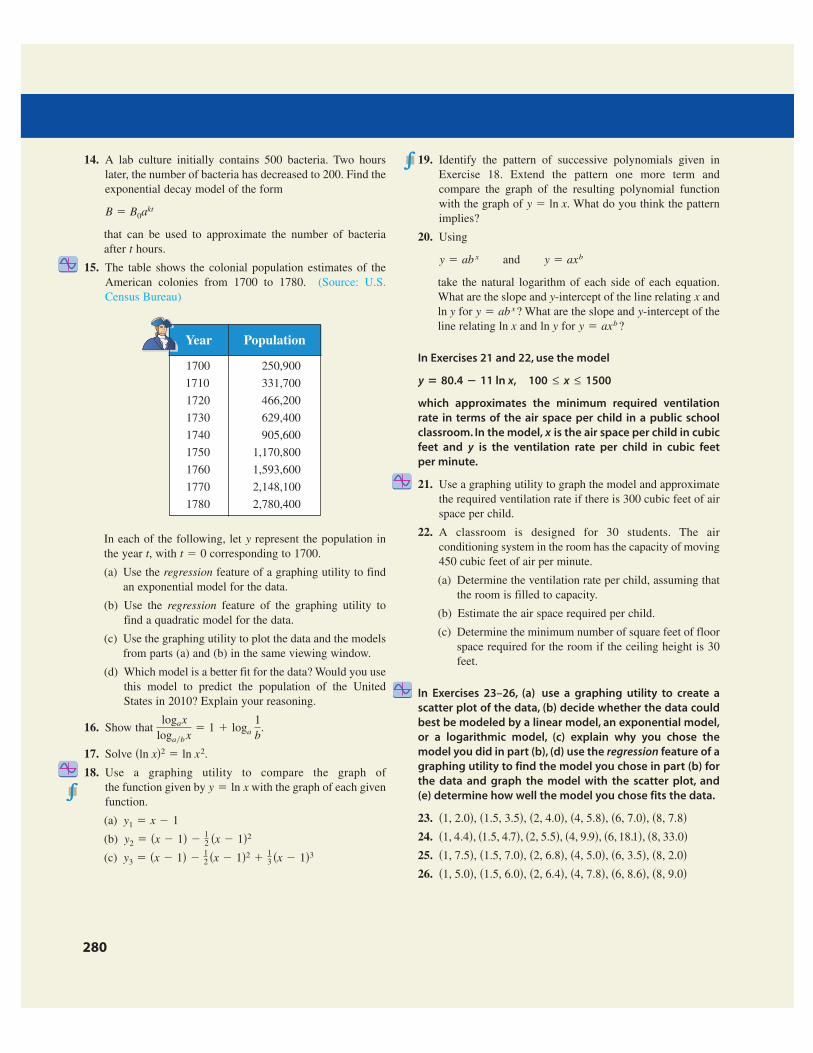
14. A lab culture initially contains 500 bacteria. Two hours
later, the number of bacteria has decreased to 200. Find the
exponential decay model of the form
that can be used to approximate the number of bacteria
after hours.
15. The table shows the colonial population estimates of the
American colonies from 1700 to 1780. (Source: U.S.
Census Bureau)
In each of the following, let represent the population in
the year with corresponding to 1700.
(a) Use the regression feature of a graphing utility to find
an exponential model for the data.
(b) Use the regression feature of the graphing utility to
find a quadratic model for the data.
(c) Use the graphing utility to plot the data and the models
from parts (a) and (b) in the same viewing window.
(d) Which model is a better fit for the data? Would you use
this model to predict the population of the United
States in 2010? Explain your reasoning.
16. Show that
17. Solve
18. Use a graphing utility to compare the graph of
the function given by with the graph of each given
function.
(a)
(b)
(c)
19. Identify the pattern of successive polynomials given in
Exercise 18. Extend the pattern one more term and
compare the graph of the resulting polynomial function
with the graph of What do you think the pattern
implies?
20. Using
and
take the natural logarithm of each side of each equation.
What are the slope and -intercept of the line relating and
for What are the slope and -intercept of the
line relating and for
In Exercises 21 and 22, use the model
which approximates the minimum required ventilation
rate in terms of the air space per child in a public school
classroom. In the model, is the air space per child in cubic
feet and is the ventilation rate per child in cubic feet
per minute.
21. Use a graphing utility to graph the model and approximate
the required ventilation rate if there is 300 cubic feet of air
space per child.
22. A classroom is designed for 30 students. The air
conditioning system in the room has the capacity of moving
450 cubic feet of air per minute.
(a) Determine the ventilation rate per child, assuming that
the room is filled to capacity.
(b) Estimate the air space required per child.
(c) Determine the minimum number of square feet of floor
space required for the room if the ceiling height is 30
feet.
In Exercises 23–26, (a) use a graphing utility to create a
scatter plot of the data, (b) decide whether the data could
best be modeled by a linear model, an exponential model,
or a logarithmic model, (c) explain why you chose the
model you did in part (b), (d) use the regression feature of a
graphing utility to find the model you chose in part (b) for
the data and graph the model with the scatter plot, and
(e) determine how well the model you chose fits the data.
23.
24.
25.
26. s1, 5.0d, s1.5, 6.0d, s2, 6.4d, s4, 7.8d, s6, 8.6d, s8, 9.0ds1, 7.5d, s1.5, 7.0d, s2, 6.8d, s4, 5.0d, s6, 3.5d, s8, 2.0ds1, 4.4d, s1.5, 4.7d, s2, 5.5d, s4, 9.9d, s6, 18.1d, s8, 33.0ds1, 2.0d, s1.5, 3.5d, s2, 4.0d, s4, 5.8d, s6, 7.0d, s8, 7.8d
y
x
100 ≤ x ≤ 1500y 5 80.4 2 11 ln x,
y 5 axb ?ln yln x
yy 5 ab x ?ln y
xy
y 5 axby 5 ab x
y 5 ln x.
y3 5 sx 2 1d 212 sx 2 1d2 1
13 sx 2 1d3
y2 5 sx 2 1d 212 sx 2 1d2
y1 5 x 2 1
y 5 ln x
sln xd2 5 ln x2.
logax
logayb x5 1 1 loga
1
b.
t 5 0t,
y
t
B 5 B0akt
280
Year Population
1700 250,900
1710 331,700
1720 466,200
1730 629,400
1740 905,600
1750 1,170,800
1760 1,593,600
1770 2,148,100
1780 2,780,400


![Math 30-1: Exponential and Logarithmic · PDF fileMath 30-1: Exponential and Logarithmic Functions ... [H+] is the ... Exponential and Logarithmic Functions Practice Exam](https://img.dokumen.tips/doc/110x75/5a7084c37f8b9abb538c080a/math-30-1-exponential-and-logarithmic-functionswwwmath30calessonslogarithmspracticeexammath30-1diplomapdf.jpg)