arX

iv:1

108.

2655

v2 [

mat

h.N

A]

8 D

ec 2

011

EXPODE - Advanced Exponential Time Integration

Toolbox for MATLAB

9. Dezember 2011

Table of Contents

1 Intoduction . . . . . . . . . . . . . . . . . . . . . . . . . . . . . . . . . . . . 3

1.1 Installation and Requirements . . . . . . . . . . . . . . . . . . . . . . 3

1.2 Quick Start . . . . . . . . . . . . . . . . . . . . . . . . . . . . . . . . 4

2 The expode Integrator . . . . . . . . . . . . . . . . . . . . . . . . . . . . . . 5

3 Using Options . . . . . . . . . . . . . . . . . . . . . . . . . . . . . . . . . . . 9

4 Available Options . . . . . . . . . . . . . . . . . . . . . . . . . . . . . . . . . 13

4.1 Options Common to All Integrators . . . . . . . . . . . . . . . . . . . 13

4.2 Options for Semilinear Integrators . . . . . . . . . . . . . . . . . . . . 17

4.3 Options for Linearized Integrators . . . . . . . . . . . . . . . . . . . . 19

4.4 Options for Constant Step Size Integrators . . . . . . . . . . . . . . . 21

4.5 Options for Variable Step Size Integrators . . . . . . . . . . . . . . . 21

5 exprk – The Exponential Runge-Kutta Integrator . . . . . . . . . . . . . . . 22

6 exprb – The Exponential Rosenbrock-type Integrator . . . . . . . . . . . . . 24

7 expmssemi – The Exponential Multistep Integrator . . . . . . . . . . . . . . 25

8 expms – The Exponential Linearized Multistep Integrator . . . . . . . . . . . 25

9 exp4 – Exponential Integrator of Order Four . . . . . . . . . . . . . . . . . . 26

10 Matrix Functions . . . . . . . . . . . . . . . . . . . . . . . . . . . . . . . . . 27

11 Writing an EXPODE Integrator . . . . . . . . . . . . . . . . . . . . . . . . . . 31

11.1 EXPODE Basics . . . . . . . . . . . . . . . . . . . . . . . . . . . . . . . 31

11.2 Integrators . . . . . . . . . . . . . . . . . . . . . . . . . . . . . . . . . 34

11.3 Options . . . . . . . . . . . . . . . . . . . . . . . . . . . . . . . . . . 37

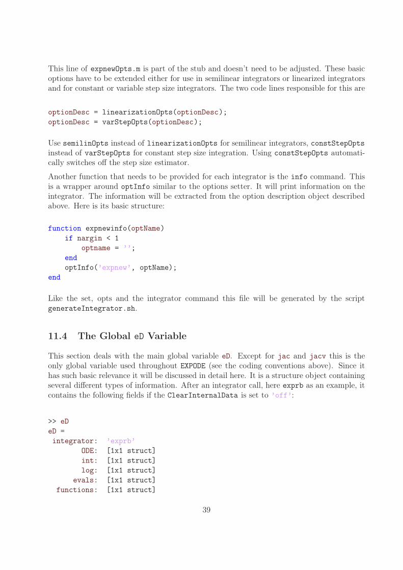
11.4 The Global eD Variable . . . . . . . . . . . . . . . . . . . . . . . . . . 39

11.5 Deploying EXPODE . . . . . . . . . . . . . . . . . . . . . . . . . . . . . 42

Literature . . . . . . . . . . . . . . . . . . . . . . . . . . . . . . . . . . . . . . . . 44

2

1 Intoduction

This document contains the documentation for the MATLAB toolbox EXPODE. The toolboxprovides advanced exponential integration methods featuring five different integrator classes,evaluation of the Matrix functions directly and by a Krylov subspace method and an adaptivestep size implementation for some of the integrators. EXPODE is as compatible as possibleto MATLAB’s internal ODE toolbox syntactically and semantically, such that a switch to thispackage is made easy.

For the mathematical details on the implementation we refer to [1]. We first give a shortquick start guide in the remainder of this section and continue with the full documentationin the next section. Note that some information might be duplicated.

1.1 Installation and Requirements

We will now describe the minimal requirements and the installation of the EXPODE toolbox.EXPODE runs on all recent and middle-aged computers. The performance highly depends onthe problem and available hardware. The toolbox was tested on MATLAB versions down toMATLAB 7.2 (R2006a), released in 2006. Older versions might be albe to run it as well and wewould appreciate feedback on success or failure. Versions prior to 7.0 cannot be compatibledue to the lack of proper function handles. OCTAVE is also not capable of running EXPODE,since it currently does not support nested functions which are used regularly in the toolbox.At

http://www.am.uni-duesseldorf.de/en/Research/03_Software.php

you can download the packages containing the EXPODE toolbox. Two different versions areavailable, a package for users and an extended one for developers. The latter contains someadditional tools helpful for extending EXPODE. Usually the user package should be sufficient.

To install, just unpack the archive obtained from the above link. In a UNIX environmentyou can do this by typing

$ tar xzvf expode-VERSION.tgz

in the directory where you downloaded the package. This will give you an expode subdirec-tory. To make it available in MATLAB, just add the package’s root to MATLAB’s path and runthe initPaths function with

>> addpath /download/path/expode;

>> initPaths;

To make a permanent installation for the current user, put the above line into your startup.mfile. See MATLAB’s help for more information.

3

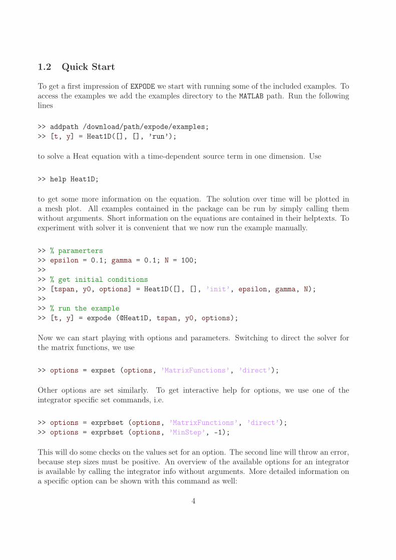
1.2 Quick Start

To get a first impression of EXPODE we start with running some of the included examples. Toaccess the examples we add the examples directory to the MATLAB path. Run the followinglines

>> addpath /download/path/expode/examples;

>> [t, y] = Heat1D([], [], ’run’);

to solve a Heat equation with a time-dependent source term in one dimension. Use

>> help Heat1D;

to get some more information on the equation. The solution over time will be plotted ina mesh plot. All examples contained in the package can be run by simply calling themwithout arguments. Short information on the equations are contained in their helptexts. Toexperiment with solver it is convenient that we now run the example manually.

>> % paramerters

>> epsilon = 0.1; gamma = 0.1; N = 100;

>>

>> % get initial conditions

>> [tspan, y0, options] = Heat1D([], [], ’init’, epsilon, gamma, N);

>>

>> % run the example

>> [t, y] = expode (@Heat1D, tspan, y0, options);

Now we can start playing with options and parameters. Switching to direct the solver forthe matrix functions, we use

>> options = expset (options, ’MatrixFunctions’, ’direct’);

Other options are set similarly. To get interactive help for options, we use one of theintegrator specific set commands, i.e.

>> options = exprbset (options, ’MatrixFunctions’, ’direct’);

>> options = exprbset (options, ’MinStep’, -1);

This will do some checks on the values set for an option. The second line will throw an error,because step sizes must be positive. An overview of the available options for an integratoris available by calling the integrator info without arguments. More detailed information ona specific option can be shown with this command as well:

4

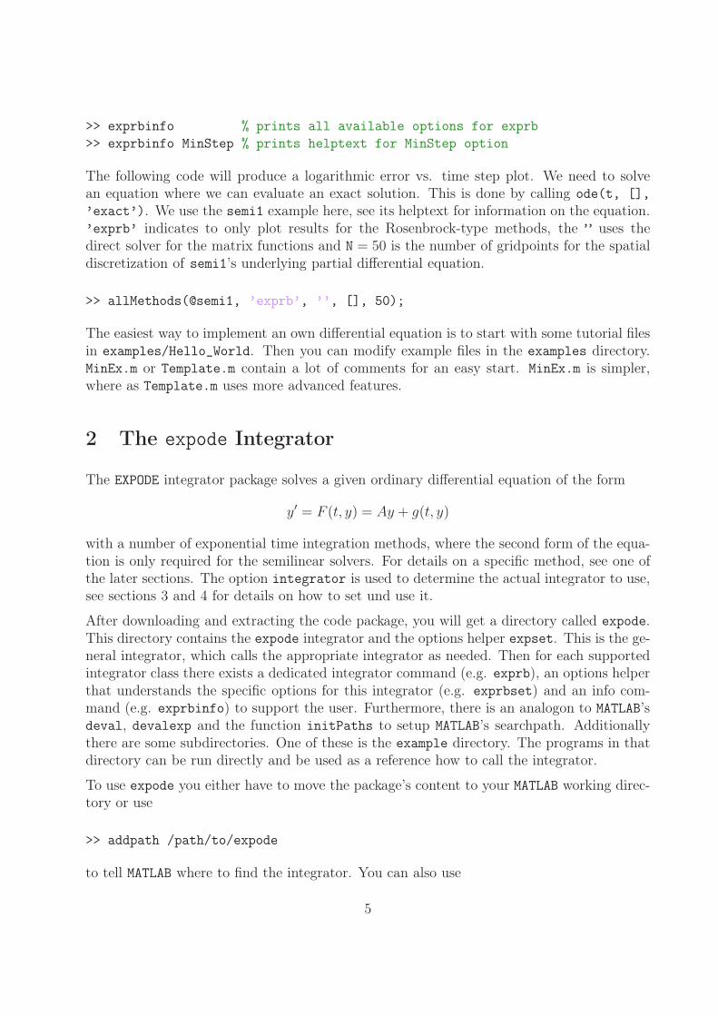
>> exprbinfo % prints all available options for exprb

>> exprbinfo MinStep % prints helptext for MinStep option

The following code will produce a logarithmic error vs. time step plot. We need to solvean equation where we can evaluate an exact solution. This is done by calling ode(t, [],

’exact’). We use the semi1 example here, see its helptext for information on the equation.’exprb’ indicates to only plot results for the Rosenbrock-type methods, the ” uses thedirect solver for the matrix functions and N = 50 is the number of gridpoints for the spatialdiscretization of semi1’s underlying partial differential equation.

>> allMethods(@semi1, ’exprb’, ’’, [], 50);

The easiest way to implement an own differential equation is to start with some tutorial filesin examples/Hello_World. Then you can modify example files in the examples directory.MinEx.m or Template.m contain a lot of comments for an easy start. MinEx.m is simpler,where as Template.m uses more advanced features.

2 The expode Integrator

The EXPODE integrator package solves a given ordinary differential equation of the form

y′ = F (t, y) = Ay + g(t, y)

with a number of exponential time integration methods, where the second form of the equa-tion is only required for the semilinear solvers. For details on a specific method, see one ofthe later sections. The option integrator is used to determine the actual integrator to use,see sections 3 and 4 for details on how to set und use it.

After downloading and extracting the code package, you will get a directory called expode.This directory contains the expode integrator and the options helper expset. This is the ge-neral integrator, which calls the appropriate integrator as needed. Then for each supportedintegrator class there exists a dedicated integrator command (e.g. exprb), an options helperthat understands the specific options for this integrator (e.g. exprbset) and an info com-mand (e.g. exprbinfo) to support the user. Furthermore, there is an analogon to MATLAB’sdeval, devalexp and the function initPaths to setup MATLAB’s searchpath. Additionallythere are some subdirectories. One of these is the example directory. The programs in thatdirectory can be run directly and be used as a reference how to call the integrator.

To use expode you either have to move the package’s content to your MATLAB working direc-tory or use

>> addpath /path/to/expode

to tell MATLAB where to find the integrator. You can also use

5

>> addpath /path/to/expode/examples

to directly run one of the examples.

expode’s user interface is adapted to MATLAB’s internal integrators. A call with all availablearguments is of the following form:

>> [t, y] = expode(@ode, {@jac}, {tspan, y0, opts}, {varargin});

To keep the explanation well-arranged, the possible call combinations will be explained stepby step. The simplest way to invoke the integrator is

>> [t, y] = expode(@ode, tspan, y0);

where ode is a function to evaluate the differential equation (and its first derivative) at givendata y and t. tspan = [t0, T] defines the integration interval. You can also use tspan =

[t0, ..., tN] for some integrators instead. This will result in a solution evaluated at thegiven times instead of the ones chosen by the integrator internally. In that case, clearly wehave t = tspan. This kind of solution is called dense output because one would typically usetspan = linspace(t0, T, N + 1) with different output data than the step selection wouldproduce. exp4 allows dense output directly as it has an own dense output formula. For allother integrators there is only a generic hermite interpolation formula which is not suitablefor stiff problems. This is disabled by default, but can be switched on via the DOGenerator

option. Use this feature with care. y0 is the initial condition to solve the equation with.

The ode function has to be callable in the following way:

>> res = ode(t, y, {flag});

t and y are the time and phase space variables respectively. flag controls the output of thefunction. An omitted or empty flag should trigger the evaluation of the right hand side.If the integrator used is for semilinear problems (exprk and expmssemi) flag = ’linop’

should trigger the evaluation of the linear part (the matrix). In case of the linearized integra-tors exprb, expms and exp4, flag can be given as flag = ’jacobian’ or flag = ’df_dt’.In the first case the derivative of the right hand side with respect to y – here called Jacobian,see the introduction – has to be evaluated at t and y. The last case is only needed if the diffe-rential equation is non-autonomous. Then ode should return the derivative of the right handside with respect to the time variable t. If the differential equation is non-autonomous, youhave to set the option NonAutonomous to ’on’, see the options section. A typical functionbody for ode is presented for a linearized integrator below.

function res = ode(t, y, flag)

if nargin == 2 || isempty(flag)

6

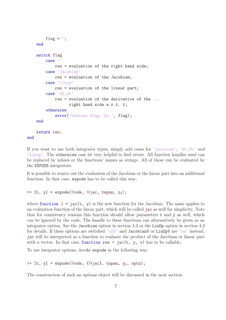
flag = ”;

end

switch flag

case ’’

res = evaluation of the right hand side;

case ’jacobian’

res = evaluation of the Jacobian;

case ’linop’

res = evaluation of the linear part;

case ’df_dt’

res = evaluation of the derivative of the ...

right hand side w.r.t. t;

otherwise

error(’Unknown flag: %s.’, flag);

end

return res;

end

If you want to use both integrator types, simply add cases for ’jacobian’, ’df_dt’ and’linop’. The otherwise case ist very helpful to find errors. All function handles used canbe replaced by inlines or the functions’ names as strings. All of these can be evaluated bythe EXPODE integrators.

It is possible to source out the evaluation of the Jacobian or the linear part into an additionalfunction. In that case, expode has to be called this way:

>> [t, y] = expode(@ode, @jac, tspan, y0);

where function J = jac(t, y) is the new function for the Jacobian. The same applies toan evaluation function of the linear part, which will be called jac as well for simplicity. Notethat for consistency reasons this function should allow parameters t and y as well, whichcan be ignored by the code. The handle to these functions can alternatively be given as anintegrator option. See the Jacobian option in section 4.3 or the LinOp option in section 4.2for details. If these options are switched ’off’ and JacobianV or LinOpV are ’on’ instead,jac will be interpreted as a function to evaluate the product of the Jacobian or linear partwith a vector. In that case, function res = jac(t, y, v) has to be callable.

To use integrator options, invoke expode in the following way:

>> [t, y] = expode(@ode, {@jac}, tspan, y0, opts);

The construction of such an options object will be discussed in the next section.

7

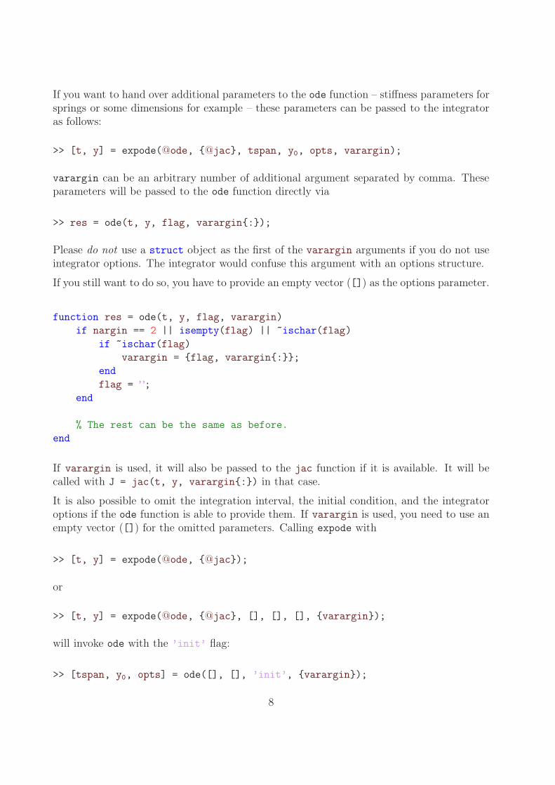
If you want to hand over additional parameters to the ode function – stiffness parameters forsprings or some dimensions for example – these parameters can be passed to the integratoras follows:

>> [t, y] = expode(@ode, {@jac}, tspan, y0, opts, varargin);

varargin can be an arbitrary number of additional argument separated by comma. Theseparameters will be passed to the ode function directly via

>> res = ode(t, y, flag, varargin{:});

Please do not use a struct object as the first of the varargin arguments if you do not useintegrator options. The integrator would confuse this argument with an options structure.

If you still want to do so, you have to provide an empty vector ([]) as the options parameter.

function res = ode(t, y, flag, varargin)

if nargin == 2 || isempty(flag) || ˜ischar(flag)

if ˜ischar(flag)

varargin = {flag, varargin{:}};

end

flag = ”;

end

% The rest can be the same as before.

end

If varargin is used, it will also be passed to the jac function if it is available. It will becalled with J = jac(t, y, varargin{:}) in that case.

It is also possible to omit the integration interval, the initial condition, and the integratoroptions if the ode function is able to provide them. If varargin is used, you need to use anempty vector ([]) for the omitted parameters. Calling expode with

>> [t, y] = expode(@ode, {@jac});

or

>> [t, y] = expode(@ode, {@jac}, [], [], [], {varargin});

will invoke ode with the ’init’ flag:

>> [tspan, y0, opts] = ode([], [], ’init’, {varargin});

8

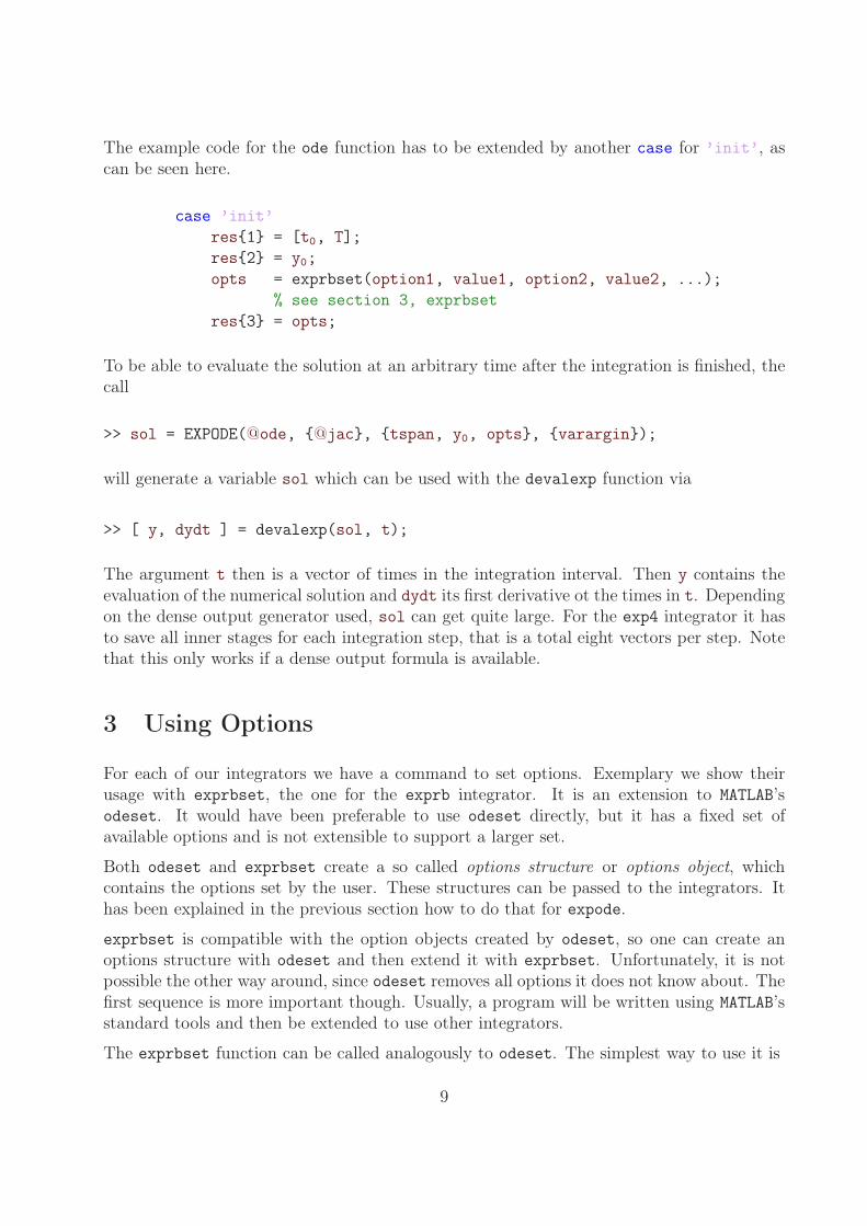
The example code for the ode function has to be extended by another case for ’init’, ascan be seen here.

case ’init’

res{1} = [t0, T];

res{2} = y0;

opts = exprbset(option1, value1, option2, value2, ...);

% see section 3, exprbset

res{3} = opts;

To be able to evaluate the solution at an arbitrary time after the integration is finished, thecall

>> sol = EXPODE(@ode, {@jac}, {tspan, y0, opts}, {varargin});

will generate a variable sol which can be used with the devalexp function via

>> [ y, dydt ] = devalexp(sol, t);

The argument t then is a vector of times in the integration interval. Then y contains theevaluation of the numerical solution and dydt its first derivative ot the times in t. Dependingon the dense output generator used, sol can get quite large. For the exp4 integrator it hasto save all inner stages for each integration step, that is a total eight vectors per step. Notethat this only works if a dense output formula is available.

3 Using Options

For each of our integrators we have a command to set options. Exemplary we show theirusage with exprbset, the one for the exprb integrator. It is an extension to MATLAB’sodeset. It would have been preferable to use odeset directly, but it has a fixed set ofavailable options and is not extensible to support a larger set.

Both odeset and exprbset create a so called options structure or options object, whichcontains the options set by the user. These structures can be passed to the integrators. Ithas been explained in the previous section how to do that for expode.

exprbset is compatible with the option objects created by odeset, so one can create anoptions structure with odeset and then extend it with exprbset. Unfortunately, it is notpossible the other way around, since odeset removes all options it does not know about. Thefirst sequence is more important though. Usually, a program will be written using MATLAB’sstandard tools and then be extended to use other integrators.

The exprbset function can be called analogously to odeset. The simplest way to use it is

9

>> opts = exprbset(option, value);

where option is an option’s name and value the user’s choice. The latter one can be scalar,vector valued, logical, a string, or a function, depending on the option chosen. All supportedoption types are listed later in this section. The info commands such as exprbinfo providedby the EXPODE package can print options supported by the EXPODE integrators.

It is also possible to pass more option-value-pairs at once and extend already existing optionobjects:

>> opts = exprbset(option1, value1, option2, value2, ...);

>> opts = exprbset(opts, option3, value3, ...);

For a more comfortable usage, you can use the integrator specific set commands (exprbset,exprkset, etc.) to check if the provided options are valid. expset itself cannot do this, sinceit does not know which integrator will be used. You can tell it by using

>> opts = exprbset(intname, {opts}, option1, value1, option2, value2, ...);

where intname is the name of the integrator, e.g. ’exprb’, ’exprk’.

In the remaining part of this section, the supported value types for options will be discussed.All of the listed types can be checked for validity by the set commands. Which type isallowed for which option is described in the next sections. The info commands in MATLAB

can provide this information.

>> exprbinfo({optname});

will display a list of all options supported by exprb if optname is omitted. If it is given,more detailed help on the specific option will be printed. Using optname = ’-’ will givethis detailed help on all options. Warning: the output is quite long, it should be used with

>> more on; exprbinfo(’-’); more off;

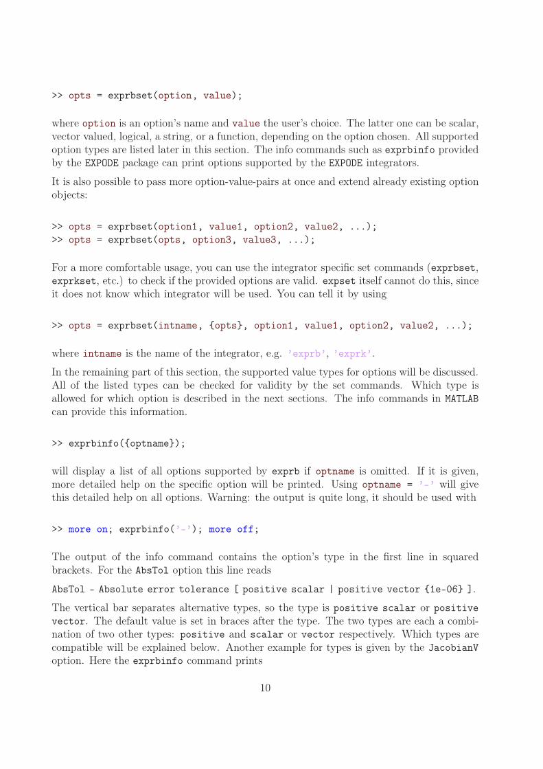
The output of the info command contains the option’s type in the first line in squaredbrackets. For the AbsTol option this line reads

AbsTol - Absolute error tolerance [ positive scalar | positive vector {1e-06} ].

The vertical bar separates alternative types, so the type is positive scalar or positive

vector. The default value is set in braces after the type. The two types are each a combi-nation of two other types: positive and scalar or vector respectively. Which types arecompatible will be explained below. Another example for types is given by the JacobianV

option. Here the exprbinfo command prints

10

JacobianV - ... [ function_handle | {’off’} | ’on’ ].

The allowed types in this case are boolean or function_handle. For types boolean and itsgeneralization list, a list of accepted values will be stated. For a boolean this list is fixedand consists of the values ’on’ (true) and ’off’ (off), for the list type the list dependson the option. The listed values are always quoted strings. Now all option types will bediscussed in detail.

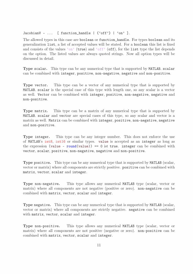
Type scalar. This type can be any numerical type that is supported by MATLAB. scalarcan be combined with integer, positive, non-negative, negative and non-positive.

Type vector. This type can be a vector of any numerical type that is supported byMATLAB. scalar is the special case of this type with length one, so any scalar is a vectoras well. Vector can be combined with integer, positive, non-negative, negative andnon-positive.

Type matrix. This type can be a matrix of any numerical type that is supported byMATLAB. scalar and vector are special cases of this type, so any scalar and vector is amatrix as well. Matrix can be combined with integer, positive, non-negative, negativeand non-positive.

Type integer. This type can be any integer number. This does not enforce the useof MATLAB’s int8, int16 or similar types. value is accepted as an integer as long asthe expression (value - round(value)) == 0 ist true. integer can be combined withvector, scalar, positive, non-negative, negative and non-positive.

Type positive. This type can be any numerical type that is supported by MATLAB (scalar,vector or matrix) where all components are strictly positive. positive can be combined withmatrix, vector, scalar and integer.

Type non-negative. This type allows any numerical MATLAB type (scalar, vector ormatrix) where all components are not negative (positive or zero). non-negative can becombined with matrix, vector, scalar and integer.

Type negative. This type can be any numerical type that is supported by MATLAB (scalar,vector or matrix) where all components are strictly negative. negative can be combinedwith matrix, vector, scalar and integer.

Type non-positive. This type allows any numerical MATLAB type (scalar, vector ormatrix) where all components are not positive (negative or zero). non-positive can becombined with matrix, vector, scalar and integer.

11

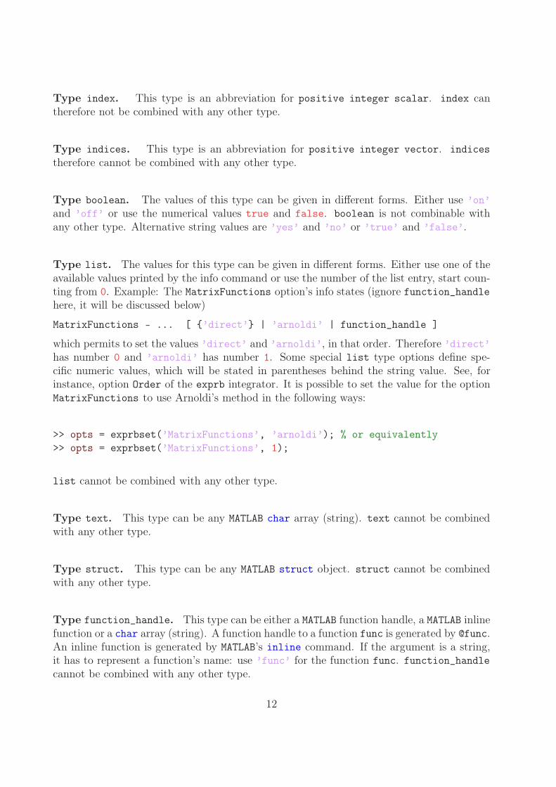
Type index. This type is an abbreviation for positive integer scalar. index cantherefore not be combined with any other type.

Type indices. This type is an abbreviation for positive integer vector. indices

therefore cannot be combined with any other type.

Type boolean. The values of this type can be given in different forms. Either use ’on’

and ’off’ or use the numerical values true and false. boolean is not combinable withany other type. Alternative string values are ’yes’ and ’no’ or ’true’ and ’false’.

Type list. The values for this type can be given in different forms. Either use one of theavailable values printed by the info command or use the number of the list entry, start coun-ting from 0. Example: The MatrixFunctions option’s info states (ignore function_handlehere, it will be discussed below)

MatrixFunctions - ... [ {’direct’} | ’arnoldi’ | function_handle ]

which permits to set the values ’direct’ and ’arnoldi’, in that order. Therefore ’direct’has number 0 and ’arnoldi’ has number 1. Some special list type options define spe-cific numeric values, which will be stated in parentheses behind the string value. See, forinstance, option Order of the exprb integrator. It is possible to set the value for the optionMatrixFunctions to use Arnoldi’s method in the following ways:

>> opts = exprbset(’MatrixFunctions’, ’arnoldi’); % or equivalently

>> opts = exprbset(’MatrixFunctions’, 1);

list cannot be combined with any other type.

Type text. This type can be any MATLAB char array (string). text cannot be combinedwith any other type.

Type struct. This type can be any MATLAB struct object. struct cannot be combinedwith any other type.

Type function_handle. This type can be either a MATLAB function handle, a MATLAB inlinefunction or a char array (string). A function handle to a function func is generated by @func.An inline function is generated by MATLAB’s inline command. If the argument is a string,it has to represent a function’s name: use ’func’ for the function func. function_handle

cannot be combined with any other type.

12

4 Available Options

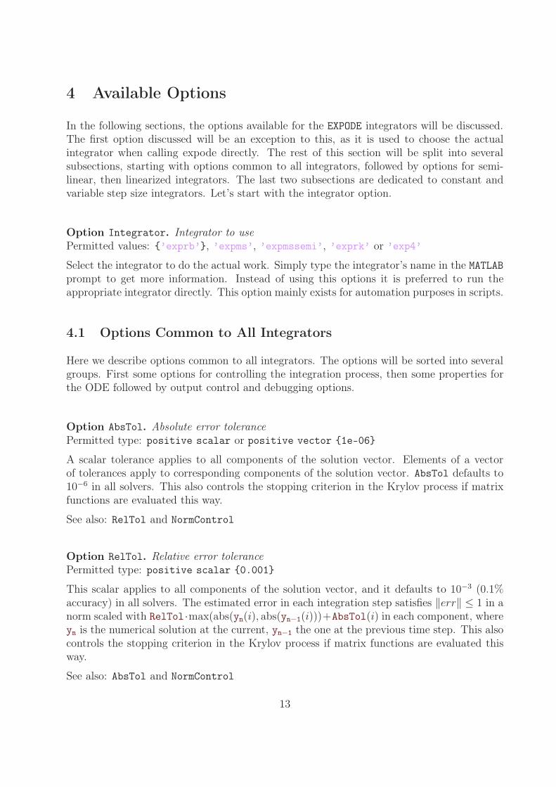
In the following sections, the options available for the EXPODE integrators will be discussed.The first option discussed will be an exception to this, as it is used to choose the actualintegrator when calling expode directly. The rest of this section will be split into severalsubsections, starting with options common to all integrators, followed by options for semi-linear, then linearized integrators. The last two subsections are dedicated to constant andvariable step size integrators. Let’s start with the integrator option.

Option Integrator. Integrator to usePermitted values: {’exprb’}, ’expms’, ’expmssemi’, ’exprk’ or ’exp4’

Select the integrator to do the actual work. Simply type the integrator’s name in the MATLABprompt to get more information. Instead of using this options it is preferred to run theappropriate integrator directly. This option mainly exists for automation purposes in scripts.

4.1 Options Common to All Integrators

Here we describe options common to all integrators. The options will be sorted into severalgroups. First some options for controlling the integration process, then some properties forthe ODE followed by output control and debugging options.

Option AbsTol. Absolute error tolerancePermitted type: positive scalar or positive vector {1e-06}

A scalar tolerance applies to all components of the solution vector. Elements of a vectorof tolerances apply to corresponding components of the solution vector. AbsTol defaults to10−6 in all solvers. This also controls the stopping criterion in the Krylov process if matrixfunctions are evaluated this way.

See also: RelTol and NormControl

Option RelTol. Relative error tolerancePermitted type: positive scalar {0.001}

This scalar applies to all components of the solution vector, and it defaults to 10−3 (0.1%accuracy) in all solvers. The estimated error in each integration step satisfies ‖err‖ ≤ 1 in anorm scaled with RelTol·max(abs(yn(i), abs(yn−1(i)))+AbsTol(i) in each component, whereyn is the numerical solution at the current, yn−1 the one at the previous time step. This alsocontrols the stopping criterion in the Krylov process if matrix functions are evaluated thisway.

See also: AbsTol and NormControl

13

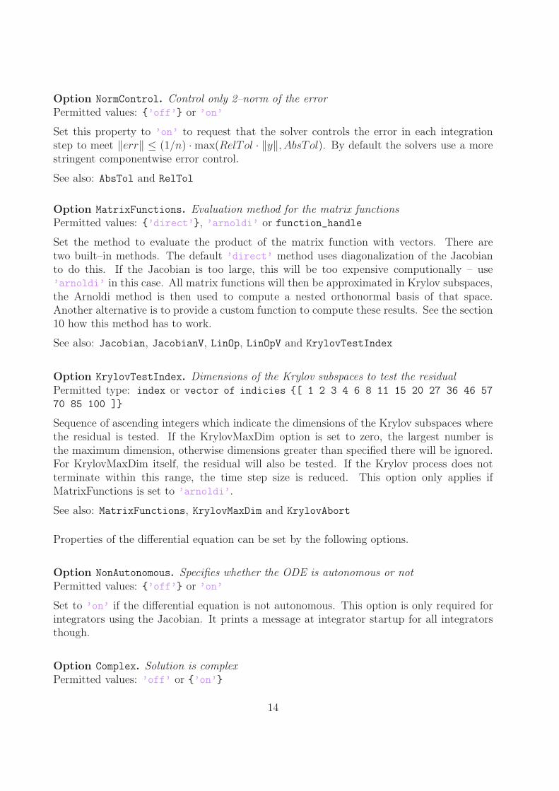
Option NormControl. Control only 2–norm of the errorPermitted values: {’off’} or ’on’

Set this property to ’on’ to request that the solver controls the error in each integrationstep to meet ‖err‖ ≤ (1/n) ·max(RelTol · ‖y‖, AbsTol). By default the solvers use a morestringent componentwise error control.

See also: AbsTol and RelTol

Option MatrixFunctions. Evaluation method for the matrix functionsPermitted values: {’direct’}, ’arnoldi’ or function_handle

Set the method to evaluate the product of the matrix function with vectors. There aretwo built–in methods. The default ’direct’ method uses diagonalization of the Jacobianto do this. If the Jacobian is too large, this will be too expensive computionally – use’arnoldi’ in this case. All matrix functions will then be approximated in Krylov subspaces,the Arnoldi method is then used to compute a nested orthonormal basis of that space.Another alternative is to provide a custom function to compute these results. See the section10 how this method has to work.

See also: Jacobian, JacobianV, LinOp, LinOpV and KrylovTestIndex

Option KrylovTestIndex. Dimensions of the Krylov subspaces to test the residualPermitted type: index or vector of indicies {[ 1 2 3 4 6 8 11 15 20 27 36 46 57

70 85 100 ]}

Sequence of ascending integers which indicate the dimensions of the Krylov subspaces wherethe residual is tested. If the KrylovMaxDim option is set to zero, the largest number isthe maximum dimension, otherwise dimensions greater than specified there will be ignored.For KrylovMaxDim itself, the residual will also be tested. If the Krylov process does notterminate within this range, the time step size is reduced. This option only applies ifMatrixFunctions is set to ’arnoldi’.

See also: MatrixFunctions, KrylovMaxDim and KrylovAbort

Properties of the differential equation can be set by the following options.

Option NonAutonomous. Specifies whether the ODE is autonomous or notPermitted values: {’off’} or ’on’

Set to ’on’ if the differential equation is not autonomous. This option is only required forintegrators using the Jacobian. It prints a message at integrator startup for all integratorsthough.

Option Complex. Solution is complexPermitted values: ’off’ or {’on’}

14

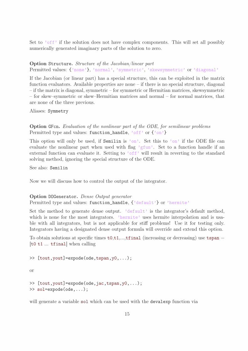
Set to ’off’ if the solution does not have complex components. This will set all possiblynumerically generated imaginary parts of the solution to zero.

Option Structure. Structure of the Jacobian/linear partPermitted values: {’none’}, ’normal’, ’symmetric’, ’skewsymmetric’ or ’diagonal’

If the Jacobian (or linear part) has a special structure, this can be exploited in the matrixfunction evaluators. Available properties are none – if there is no special structure, diagonal– if the matrix is diagonal, symmetric – for symmetric or Hermitian matrices, skewsymmetric– for skew–symmetric or skew–Hermitian matrices and normal – for normal matrices, thatare none of the three previous.

Aliases: Symmetry

Option GFcn. Evaluation of the nonlinear part of the ODE, for semilinear problemsPermitted type and values: function_handle, ’off’ or {’on’}

This option will only be used, if Semilin is ’on’. Set this to ’on’ if the ODE file canevaluate the nonlinear part when used with flag ’gfun’. Set to a function handle if anexternal function can evaluate it. Setting to ’off’ will result in reverting to the standardsolving method, ignoring the special structure of the ODE.

See also: Semilin

Now we will discuss how to control the output of the integrator.

Option DOGenerator. Dense Output generatorPermitted type and values: function_handle, {’default’} or ’hermite’

Set the method to generate dense output. ’default’ is the integrator’s default method,which is none for the most integrators. ’hermite’ uses hermite interpolation and is usa-ble with all integrators, but is not applicable for stiff problems! Use it for testing only.Integrators having a designated dense output formula will override and extend this option.

To obtain solutions at specific times t0,t1,...,tfinal (increasing or decreasing) use tspan =[t0 t1 ... tfinal] when calling

>> [tout,yout]=expode(ode,tspan,y0,...);

or

>> [tout,yout]=expode(ode,jac,tspan,y0,...);

>> sol=expode(ode,...);

will generate a variable sol which can be used with the devalexp function via

15

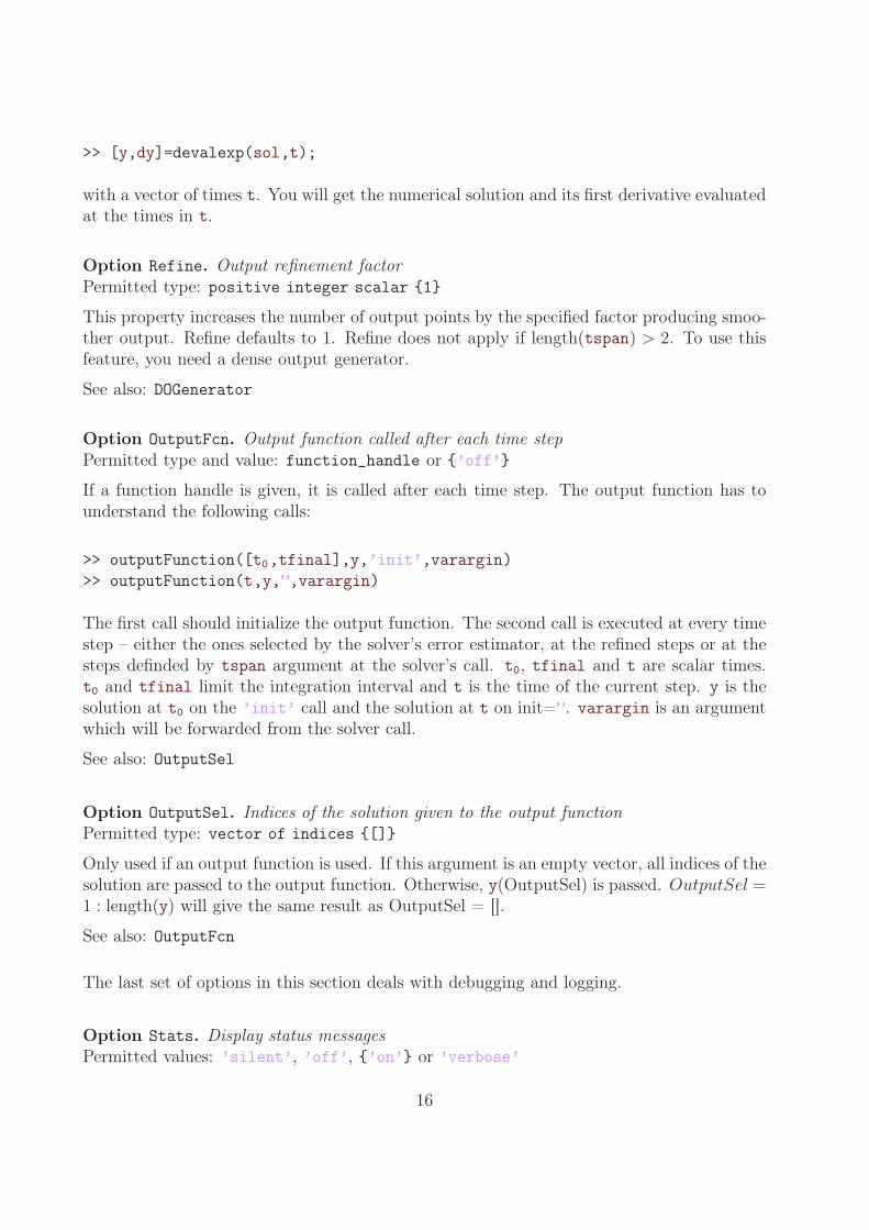
>> [y,dy]=devalexp(sol,t);

with a vector of times t. You will get the numerical solution and its first derivative evaluatedat the times in t.

Option Refine. Output refinement factorPermitted type: positive integer scalar {1}

This property increases the number of output points by the specified factor producing smoo-ther output. Refine defaults to 1. Refine does not apply if length(tspan) > 2. To use thisfeature, you need a dense output generator.

See also: DOGenerator

Option OutputFcn. Output function called after each time stepPermitted type and value: function_handle or {’off’}

If a function handle is given, it is called after each time step. The output function has tounderstand the following calls:

>> outputFunction([t0,tfinal],y,’init’,varargin)

>> outputFunction(t,y,”,varargin)

The first call should initialize the output function. The second call is executed at every timestep – either the ones selected by the solver’s error estimator, at the refined steps or at thesteps definded by tspan argument at the solver’s call. t0, tfinal and t are scalar times.t0 and tfinal limit the integration interval and t is the time of the current step. y is thesolution at t0 on the ’init’ call and the solution at t on init=”. varargin is an argumentwhich will be forwarded from the solver call.

See also: OutputSel

Option OutputSel. Indices of the solution given to the output functionPermitted type: vector of indices {[]}

Only used if an output function is used. If this argument is an empty vector, all indices of thesolution are passed to the output function. Otherwise, y(OutputSel) is passed. OutputSel =1 : length(y) will give the same result as OutputSel = [].

See also: OutputFcn

The last set of options in this section deals with debugging and logging.

Option Stats. Display status messagesPermitted values: ’silent’, ’off’, {’on’} or ’verbose’

16

Set the level of status messages printed by the integrator. If JacobianStats, StepStats

and MatrixFunctionLog are set to ’auto’, they will be activated only when Stats is setto ’verbose’ and be deactivated on all other settings. Setting this option to ’silent’ willalso disable warnings.

See also: JacobianStats, StepStats and MatrixFunctionStats

Option MatrixFunctionStats. Display status messages for matrix function evaluationsPermitted values: ’off’, ’on’ or {’auto’}

Control, whether or not to display status messages for the matrix function evaluations. Whenset to auto, this will be activated when Stats is set to ’verbose’.

See also: Stats

Option Waitbar. Show a waitbar to display progressPermitted values: {’off’}, ’on’, ’text’ or ’both’

Set to ’on’ to display the current progress after each time step. Set to ’text’ if you wantto display the progess on the MATLAB prompt. Set to ’both’ if you want both kind ofdisplays.

See also: Stats

Option ClearInternalData. Clear internal integrator dataPermitted values: ’off’ or {’on’}

Set to ’off’ if you want to keep the integrator’s internal data. This data is available in theglobal eD variable.

4.2 Options for Semilinear Integrators

In this subsection we will discuss options common to the semilinear integrators exprk andexpmssemi. To evaluate the linear operator we have the following two options.

Option LinOp. Evaluation function for the ODE’s right hand side’s linear partPermitted type and values: function_handle, ’off’, {’on’} or matrix

The integrator needs to compute matrix functions with the linear part of the right handside of the ODE. Therefore, either the linear part has to be evaluated, or the evaluationof the linear part times vector has to be provided – this only works when using Krylovapproximations to the matrix functions. If this option is set to ’on’ (default), the ode

function will be called with

>> lin=ode(t,y,’linop’,varargin);

17

If it is a function handle, the call

>> lp=opts.LinOp; lin=lp(t,y,varargin);

will be executed. Note that the linear part will only be evaluated once.

See also: LinOpV and MatrixFunctions

Aliases: Jacobian

Option LinOpV. Evaluation function for the ODE’s right hand side’s linear part times vectorPermitted type and values: function_handle, {’off’} or ’on’

When using Krylov approximations to the matrix functions of the linear part of the righthand side times vectors, this option can be used to provide the result of the computation ofthe linear part multiplied by a vector. Sometimes it is faster to compute this directly insteadof computing the full linear part. If this option is set to ’on’ (default), the ODE functionwill be called with

>> res=ode(t,y,’linpop_v’,v,varargin);

If it is a function handle, the call

>> lpv=opts.LinOpV; res=lpv(t,y,v,varargin);

will be executed.

See also: LinOp and MatrixFunctions

Aliases: JacobianV

Additionally you can control the logging output with this option.

Option LinOpStats. Display status messages for the evaluation of the linear partPermitted values: ’off’, ’on’ or {’auto’}

Control, whether or not to display status messages for the evaluation of the linear part.When set to auto, this will be activated when Stats is set to ’verbose’. If enabled, thisoptions prints

>> Evaluating linear part ... done

when the linear part is evaluated. If option Stats set to ’verbose’ the Eigenvalues of thelinear part will be plotted additionally.

See also: Stats

Aliases: JacobianStats

18

4.3 Options for Linearized Integrators

In this subsection we will discuss options common to the linearized integrators exprb, expmsand exp4. Again the options are split into smaller groups to keep the information clearly pre-sented. The first couple of options deal with the evaluation of the needed data. Additionallywe have one additional option for the equation’s properties and one for logging.

Option Jacobian. Evaluation function for the ODE’s right hand side’s JacobianPermitted type and values: function_handle, ’off’, {’on’} or matrix

The integrator needs to compute matrix functions with the Jacobian of the right handside of the ODE. Therefore, either the Jacobian has to be evaluated, or the evaluation of theJacobian times vector has to be provided – this only works when using Krylov approximationsto the matrix functions. If this option is set to ’on’ (default), the ode function will be calledwith

>> j=ode(t,y,’jacobian’,varargin);

If it is a function handle, the call

>> jac=opts.Jacobian; j=jac(t,y,varargin);

will be executed. If the Jacobian is constant, set this option to the constant matrix.

See also: JacobianV and MatrixFunctions

Aliases: LinOp

Option JacobianV. Evaluation function for the ODE’s right hand side’s Jacobian timesvectorPermitted type and values: function_handle, {’off’} or ’on’

When using Krylov approximations to the matrix functions of the Jacobian of the right handside times vectors, this option can be used to provide the result of the computation of theJacobian multiplied by a vector. Sometimes it is faster to compute this directly instead ofcomputing the full Jacobian. If this option is set to ’on’ (default), the ODE function willbe called with

>> res=ode(t,y,’jacobian_v’,v,varargin);

If it is a function handle, the call

>> jacv=opts.JacobianV; res=jacv(t,y,v,varargin);

19

will be executed.

See also: Jacobian and MatrixFunctions

Aliases: LinOpV

Option GJacobian. Evaluation of the Jacobian of the nonlinear part of the ODE, forsemilinear problemsPermitted type and values: function_handle, ’off’ or {’on’}

This option will only be used if Semilin is ’on’. Set this to ’on’ if the ODE file canevaluate the Jacobian of the nonlinear part when used with flag ’dg_dy’. Set to a functionhandle if an external function can evaluate it. Setting this to ’off’, you will need to useKrylov approximations to the matrix functions and set the GJacobianV to something elsethan ’off’.

See also: Semilin, GJacobianV and MatrixFunctions

Option GJacobianV. Evaluation of the Jacobian of the nonlinear part of the ODE timesvector, for semilinear problemsPermitted type and values: function_handle, {’off’} or ’on’

This option will only be used if Semilin is ’on’ and MatrixFunctions is not ’direct’.Set this to ’on’ if the ODE file can evaluate the product of the Jacobian of the nonlinearpart with a vector when used with flag ’dg_dy_v’. Set to a function handle if an externalfunction can evaluate it. Setting to ’off’ will use GJacobian.

See also: Semilin, GJacobian and MatrixFunctions

The differential equation can now have this additional property.

Option Semilin. Specifies whether the ODE is semilinearPermitted values: {’off’} or ’on’

Set to ’on’, if the differential equation has the form

y′ = Ay + g(t, y)

Then add the flags ’gfun’ and ’dg_dy’ to your ODE file to evaluate the non–linear partg and its derivative with respect to y. Alternatively, you can use the GFun and GJacobian

options to set these. If you use Krylov approximations to the matrix exponentials, youcan also add the flag ’dg_dy_v’ to evaluate the Jacobian of g times a vector or use theGJacobianV option to do so.

See also: GFcn, GJacobian, GJacobianV, MatrixFunctions and JacobianV

Please note that for the semilinear integrators in the next section this option is alwaysassumed ’on’.

20

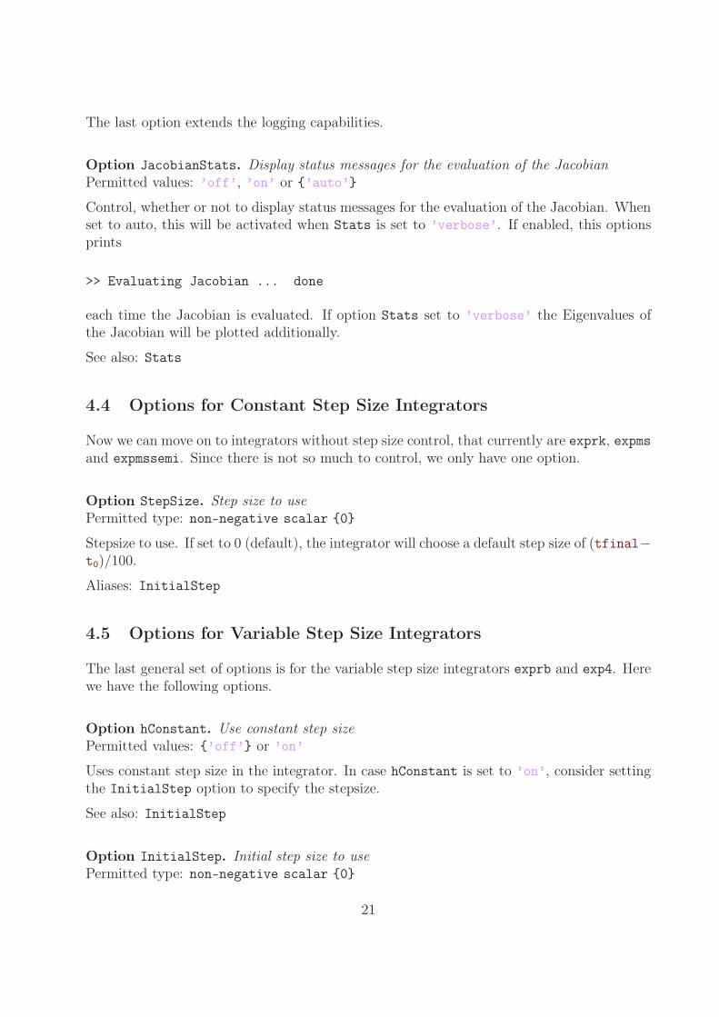
The last option extends the logging capabilities.

Option JacobianStats. Display status messages for the evaluation of the JacobianPermitted values: ’off’, ’on’ or {’auto’}

Control, whether or not to display status messages for the evaluation of the Jacobian. Whenset to auto, this will be activated when Stats is set to ’verbose’. If enabled, this optionsprints

>> Evaluating Jacobian ... done

each time the Jacobian is evaluated. If option Stats set to ’verbose’ the Eigenvalues ofthe Jacobian will be plotted additionally.

See also: Stats

4.4 Options for Constant Step Size Integrators

Now we can move on to integrators without step size control, that currently are exprk, expmsand expmssemi. Since there is not so much to control, we only have one option.

Option StepSize. Step size to usePermitted type: non-negative scalar {0}

Stepsize to use. If set to 0 (default), the integrator will choose a default step size of (tfinal−t0)/100.

Aliases: InitialStep

4.5 Options for Variable Step Size Integrators

The last general set of options is for the variable step size integrators exprb and exp4. Herewe have the following options.

Option hConstant. Use constant step sizePermitted values: {’off’} or ’on’

Uses constant step size in the integrator. In case hConstant is set to ’on’, consider settingthe InitialStep option to specify the stepsize.

See also: InitialStep

Option InitialStep. Initial step size to usePermitted type: non-negative scalar {0}

21

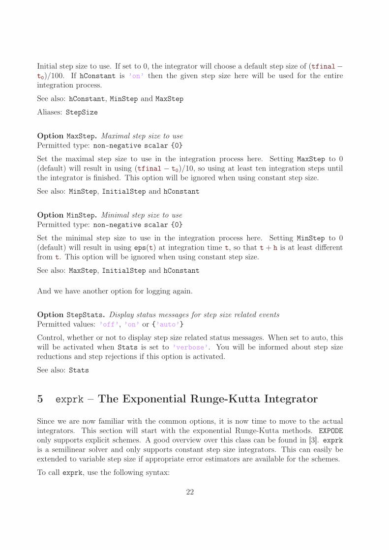
Initial step size to use. If set to 0, the integrator will choose a default step size of (tfinal−t0)/100. If hConstant is ’on’ then the given step size here will be used for the entireintegration process.

See also: hConstant, MinStep and MaxStep

Aliases: StepSize

Option MaxStep. Maximal step size to usePermitted type: non-negative scalar {0}

Set the maximal step size to use in the integration process here. Setting MaxStep to 0(default) will result in using (tfinal − t0)/10, so using at least ten integration steps untilthe integrator is finished. This option will be ignored when using constant step size.

See also: MinStep, InitialStep and hConstant

Option MinStep. Minimal step size to usePermitted type: non-negative scalar {0}

Set the minimal step size to use in the integration process here. Setting MinStep to 0(default) will result in using eps(t) at integration time t, so that t + h is at least differentfrom t. This option will be ignored when using constant step size.

See also: MaxStep, InitialStep and hConstant

And we have another option for logging again.

Option StepStats. Display status messages for step size related eventsPermitted values: ’off’, ’on’ or {’auto’}

Control, whether or not to display step size related status messages. When set to auto, thiswill be activated when Stats is set to ’verbose’. You will be informed about step sizereductions and step rejections if this option is activated.

See also: Stats

5 exprk – The Exponential Runge-Kutta Integrator

Since we are now familiar with the common options, it is now time to move to the actualintegrators. This section will start with the exponential Runge-Kutta methods. EXPODE

only supports explicit schemes. A good overview over this class can be found in [3]. exprk

is a semilinear solver and only supports constant step size integrators. This can easily beextended to variable step size if appropriate error estimators are available for the schemes.

To call exprk, use the following syntax:

22

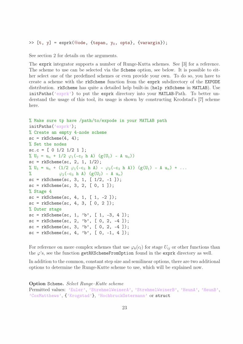
>> [t, y] = exprk(@ode, {tspan, y0, opts}, {varargin});

See section 2 for details on the arguments.

The exprk integrator supports a number of Runge-Kutta schemes. See [3] for a reference.The scheme to use can be selected via the Scheme option, see below. It is possible to eit-her select one of the predefined schemes or even provide your own. To do so, you have tocreate a scheme with the rkScheme function from the exprk subdirectory of the EXPODE

distribution. rkScheme has quite a detailed help built-in (help rkScheme in MATLAB). UseinitPaths(’exprk’) to put the exprk directory into your MATLAB-Path. To better un-derstand the usage of this tool, its usage is shown by constructing Krodstad’s [7] schemehere.

% Make sure tp have /path/to/expode in your MATLAB path

initPaths(’exprk’);

% Create an empty 4-node scheme

sc = rkScheme(4, 4);

% Set the nodes

sc.c = [ 0 1/2 1/2 1 ];

% U2 = un + 1/2 ϕ1(-c2 h A) (g(U1) - A un))

sc = rkScheme(sc, 2, 1, 1/2);

% U3 = un + (1/2 ϕ1(-c3 h A) - ϕ2(-c3 h A)) (g(U1) - A un) + ...

% ϕ2(-c3 h A) (g(U2) - A un)

sc = rkScheme(sc, 3, 1, [ 1/2, -1 ]);

sc = rkScheme(sc, 3, 2, [ 0, 1 ]);

% Stage 4

sc = rkScheme(sc, 4, 1, [ 1, -2 ]);

sc = rkScheme(sc, 4, 3, [ 0, 2 ]);

% Outer stage

sc = rkScheme(sc, 1, ’b’, [ 1, -3, 4 ]);

sc = rkScheme(sc, 2, ’b’, [ 0, 2, -4 ]);

sc = rkScheme(sc, 3, ’b’, [ 0, 2, -4 ]);

sc = rkScheme(sc, 4, ’b’, [ 0, -1, 4 ]);

For reference on more complex schemes that use ϕk(cl) for stage Uij or other functions thanthe ϕ’s, see the function getRKSchemeFromOption found in the exprk directory as well.

In addition to the common, constant step size and semilinear options, there are two additionaloptions to determine the Runge-Kutte scheme to use, which will be explained now.

Option Scheme. Select Runge–Kutte schemePermitted values: ’Euler’, ’StrehmelWeinerA’, ’StrehmelWeinerB’, ’HeunA’, ’HeunB’,’CoxMatthews’, {’Krogstad’}, ’HochbruckOstermann’ or struct

23

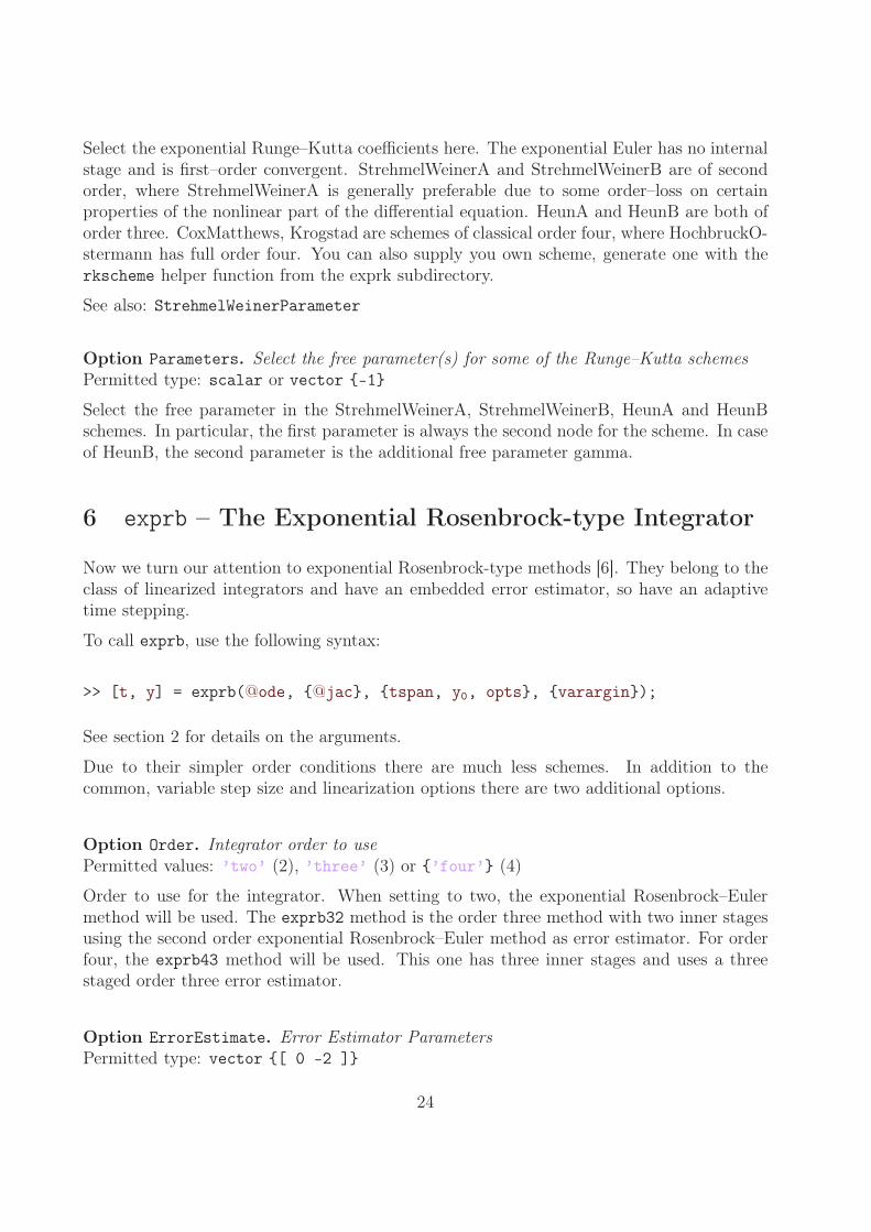
Select the exponential Runge–Kutta coefficients here. The exponential Euler has no internalstage and is first–order convergent. StrehmelWeinerA and StrehmelWeinerB are of secondorder, where StrehmelWeinerA is generally preferable due to some order–loss on certainproperties of the nonlinear part of the differential equation. HeunA and HeunB are both oforder three. CoxMatthews, Krogstad are schemes of classical order four, where HochbruckO-stermann has full order four. You can also supply you own scheme, generate one with therkscheme helper function from the exprk subdirectory.

See also: StrehmelWeinerParameter

Option Parameters. Select the free parameter(s) for some of the Runge–Kutta schemesPermitted type: scalar or vector {-1}

Select the free parameter in the StrehmelWeinerA, StrehmelWeinerB, HeunA and HeunBschemes. In particular, the first parameter is always the second node for the scheme. In caseof HeunB, the second parameter is the additional free parameter gamma.

6 exprb – The Exponential Rosenbrock-type Integrator

Now we turn our attention to exponential Rosenbrock-type methods [6]. They belong to theclass of linearized integrators and have an embedded error estimator, so have an adaptivetime stepping.

To call exprb, use the following syntax:

>> [t, y] = exprb(@ode, {@jac}, {tspan, y0, opts}, {varargin});

See section 2 for details on the arguments.

Due to their simpler order conditions there are much less schemes. In addition to thecommon, variable step size and linearization options there are two additional options.

Option Order. Integrator order to usePermitted values: ’two’ (2), ’three’ (3) or {’four’} (4)

Order to use for the integrator. When setting to two, the exponential Rosenbrock–Eulermethod will be used. The exprb32 method is the order three method with two inner stagesusing the second order exponential Rosenbrock–Euler method as error estimator. For orderfour, the exprb43 method will be used. This one has three inner stages and uses a threestaged order three error estimator.

Option ErrorEstimate. Error Estimator ParametersPermitted type: vector {[ 0 -2 ]}

24

The order four integrator uses an error estimator that can be tweaked with two parametersa and b. These two parameters can be specified here with ErrorEstimate = [a, b]. Chooseb 6= 1− 6a, otherwise the error estimator gets close to weak order four instead of three.

7 expmssemi – The Exponential Multistep Integrator

This section discusses the exponential multistep integrator expmssemi, cf. [8] and [4]. Aswith exponential Runge-Kutta methods it’s a semilinear solver and only supports constantstep sizes. In contrast to these methods, it is much harder to generalize them to variablestep sizes due to their construction.

To call expmssemi, use the following syntax:

>> [t, y] = expmssemi(@ode, {tspan, y0, opts}, {varargin});

See section 2 for details on the arguments.

In addition to the common, constant step size and semilinear options there is one additionaloption to determine the step count.

Option kStep. Number of old time steps to usePermitted values: ’one’ (1), ’two’ (2), ’three’ (3), {’four’} (4), ’five’ (5) or ’six’

(6)

Number of old time steps the method should use. One gives the exponential Euler method,which is first order convergent. The number of steps is automatically the order of the schemeas well.

Option StartupSteps. Source of the startup steps needed for the multi step methodPermitted values: {’Fixpoint’}, ’Exact’ or ’ExpRK’

Select the computation method for the startup steps for the multistep method. ’Fixpoint’uses a fixedpoint iteration to compute the steps. ’Exact’ queries the ODE with the flag’exact’. ’ExpRK’ uses an exponential Runge–Kutta scheme of the appropriate order. Notethat only methods up to order five are possible this way.

8 expms – The Exponential Linearized Multistep Integra-

tor

This section discusses the exponential linearized multistep integrator expms. It is a linearizedvariant of the expmssemi and only supports constant step sizes. We have implemented the

25

general scheme introduced by Hochbruck and Ostermann in [5] and a scheme proposed byTokman in [9].

To call expms, use the following syntax:

>> [t, y] = expms(@ode, {@jac}, {tspan, y0, opts}, {varargin});

See section 2 for details on the arguments.

In addition to the common, constant step size and linearization options there is one additionaloption to determine the integration scheme.

Option kStep. Number of old time steps to usePermitted values: ’one’ (1), ’two’ (2), ’three’ (3), {’four’} (4), ’five’ (5) or ’Tokman’(6)

Number of old time steps the method should use. One gives the exponential Rosenbrock–Euler method, which is second order convergent. The number of steps plus one is auto-matically the order of the scheme as well. The ’Tokman’ two step scheme was proposedearlier than the more general construction by Hochbruck and Ostermann and is third orderconvergent.

Option StartupSteps. Source of the startup steps needed for the multi step methodPermitted values: {’Fixpoint’}, ’Exact’ or ’ExpRB’

Select the computation method for the startup steps for the multistep method. ’Fixpoint’uses a fixedpoint iteration to compute the steps. ’Exact’ queries the ODE with the flag’exact’. ’ExpRB’ uses an exponential Rosenbrock–type scheme of the appropriate order.Note that only methods up to order five are possible this way.

9 exp4 – Exponential Integrator of Order Four

This section is dedicated to the exp4 integrator [2]. It belongs to the class of linearizedintegrators and has adaptive time stepping.

To call exp4, use the following syntax:

>> [t, y] = exp4(@ode, {@jac}, {tspan, y0, opts}, {varargin});

See section 2 for details on the arguments.

Since exp4 has its own dense output formula, it overrides the DOGenerator option.

26

Option DOGenerator. Dense Output generatorPermitted type and values: function_handle, {’exp4’}, ’hermite’ or ’none’

Set the method to generate dense output. Default is ’exp4’, exp4’s own dense outputformula. It can be overriden to use hermite interpolation by setting this option to ’hermite’.Hermite interpolation is not applicable for stiff problems. Use it for testing only. Additionallythe dense output generator can be switched off.

10 Matrix Functions

This section deals with custom evaluation functions for the product of matrix functions withvectors.

expode has two built-in methods to compute these evaluations: directly by diagonalisationand using a Krylov subspace method. In some situations, it can be useful to provide acustom function that does this job. If the Jacobian has a special structure that makes itpossible to compute matrix exponentials differently even in large dimensions, this would besuch a case. For this reason, it is possible to hook an arbitrary function into the integrationprocess. See the MatrixFunctions option on how to accomplish that.

The two internal functions are implemented the same way as an external method would haveto work. They can be used for reference and can be found in the EXPODE distribution atmatFun/matFunDirect.m and matFun/matFunKrylov.m. The former one is much easier tounderstand due to its size and complexity.

It will be neccessary to use the global eD, jac and gjac variables which contain informa-tion shared between the various EXPODE functions. See subsection 11.4 for details on thesevariables. The parts important for this context will be explained when they appear.

All logging output of the function should be printed with the eD.log.matFunLog function.This way it can easily be redirected or disabled by the integrator.

The custom function will be called matFun in the remainder of this section. It will beinvoked in different ways by the EXPODE integrators. The function’s signature needs to havethe following form:

function [ h, varargout ] = ...

matFun(job, t, y, h, flag, v, reusable, reuse, facs)

global eD;

o = eD.int.o;

funs = eD.functions;

The flag variable has two different roles. It can either request a specific action to beperformed or it can inform the method about the meaning of the currently evaluated matrixfunction. The request-type flags will be discussed first.

27

>> matFun([], [], [], [], ’init’);

should initialize the function globally. It has to state whether or not it requires to explicitlyevaluate the Jacobian of the right hand side and – if used – the one of the non-linear part gfor semilinear problems (see option Semilin). This is done by setting

eD.matFun.needJacExplicit = true;

eD.matFun.needGJacExplicit = true;

or to false respectively. The direct solver for instance sets both values to true, since itdiagonalizes the Jacobian, the Krylov method sets it so false, since it only needs to evaluatethe product of the Jacobian with a vector. If the first variable is true, then the global jacvariable contains the evaluation of the Jacobian at the current step. gjac contains theevaluation of g’s Jacobian.

Additionally, all statistical data fields have to be initialized. They are later used with the’statistics’ flag. Example: the direct evaluator sets

eD.stats.matFun.NofDiag = 0;

eD.stats.matFun.NofMFEv = 0;

These two variables count the number of matrix function evaluations and the number ofdiagonalizations of the Jacobian.

We continue with the registerjobs phase. It will be called, after the solver step decides whichmatrix functions it needs to evaluate. This can be in two situations: Either after the matrixfunction evaluator was initialized with the ’init’ flag and now has enough informationabout the differential equation and the options, or when the integration scheme requires achange of the matrix function coefficients or even exchanges some matrix functions. Thelatter can be the case for instance in the multistep integrators, after their startup phase isfinished and the normal integration routine is started. The registerjobs phase is triggered by

>> matFun(jobs, [], [], [], ’registerjobs’);

The jobs variable is a struct of vectors or matrices. The fieldnames of this struct representthe meaning of the vector to multiply the matrix function with. Typically ’F’ is used for aproduct with the right hand side, and ’v’ for the non-autonomous correction. Let job be afield of jobs. Each row of the matrix job contains the coefficients for a linear combination ofthe matrix functions in eD.int.jobFunctions. eD.int.jobFunctions contains the scalar,vectorized versions of the matrix functions. For exprb it is constructed the following way:

eD.int.jobFunctions = {

@phi1

28

@phi2

@phi3

@phi4

@(A, h) phi1(A, h/2)

@(A, h) phi2(A, h/2)

};

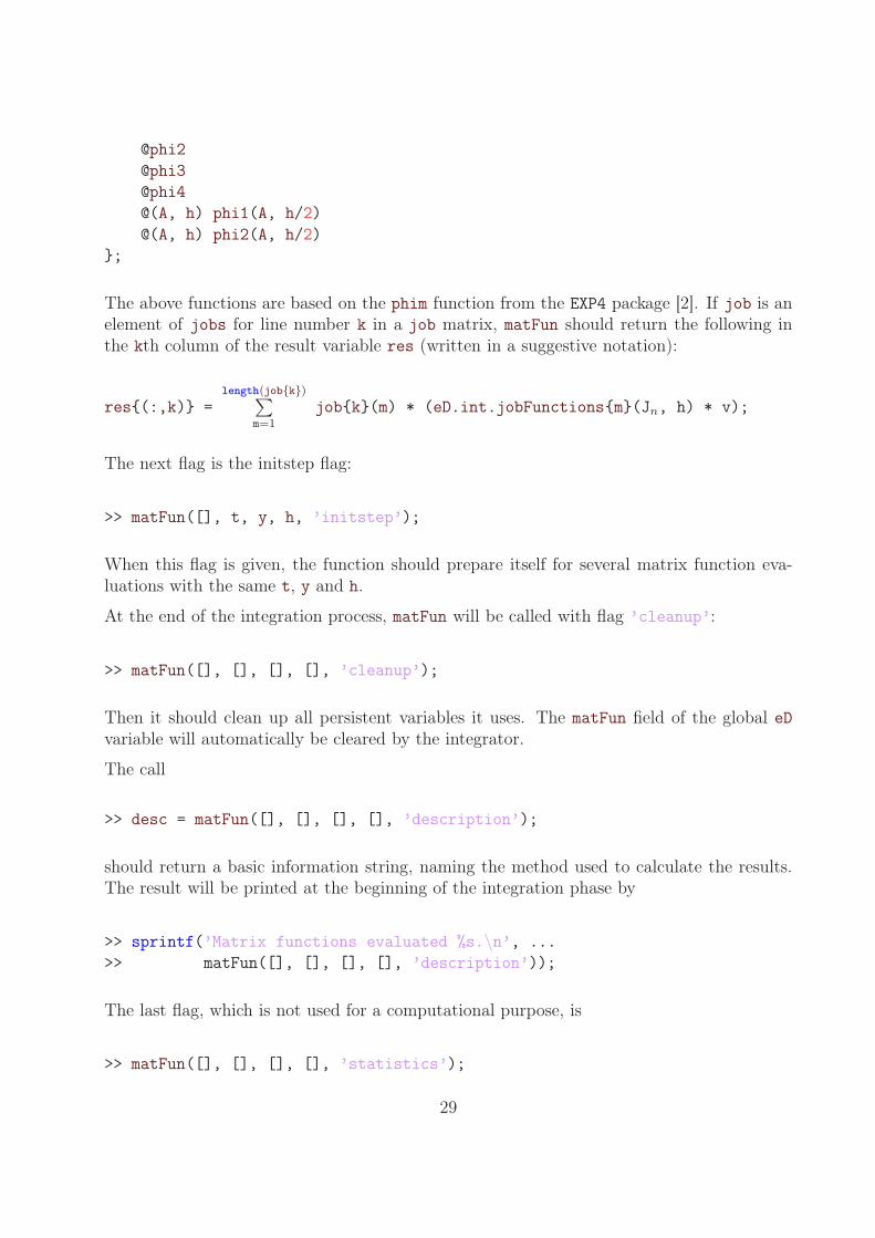
The above functions are based on the phim function from the EXP4 package [2]. If job is anelement of jobs for line number k in a job matrix, matFun should return the following inthe kth column of the result variable res (written in a suggestive notation):

res{(:,k)} =length(job{k})∑

m=1

job{k}(m) * (eD.int.jobFunctions{m}(Jn, h) * v);

The next flag is the initstep flag:

>> matFun([], t, y, h, ’initstep’);

When this flag is given, the function should prepare itself for several matrix function eva-luations with the same t, y and h.

At the end of the integration process, matFun will be called with flag ’cleanup’:

>> matFun([], [], [], [], ’cleanup’);

Then it should clean up all persistent variables it uses. The matFun field of the global eDvariable will automatically be cleared by the integrator.

The call

>> desc = matFun([], [], [], [], ’description’);

should return a basic information string, naming the method used to calculate the results.The result will be printed at the beginning of the integration phase by

>> sprintf(’Matrix functions evaluated %s.\n’, ...

>> matFun([], [], [], [], ’description’));

The last flag, which is not used for a computational purpose, is

>> matFun([], [], [], [], ’statistics’);

29

Then matFun is expected to print some statistics. See the ’init’ flag above for an exampleon what the direct method logs. If there are no interesting statistical data collected, thisflag should be ignored.

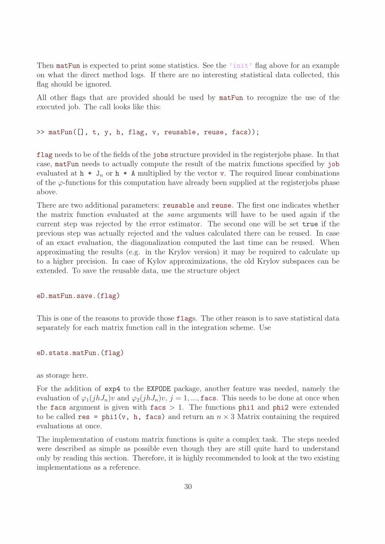
All other flags that are provided should be used by matFun to recognize the use of theexecuted job. The call looks like this:

>> matFun([], t, y, h, flag, v, reusable, reuse, facs));

flag needs to be of the fields of the jobs structure provided in the registerjobs phase. In thatcase, matFun needs to actually compute the result of the matrix functions specified by job

evaluated at h * Jn or h * A multiplied by the vector v. The required linear combinationsof the ϕ-functions for this computation have already been supplied at the registerjobs phaseabove.

There are two additional parameters: reusable and reuse. The first one indicates whetherthe matrix function evaluated at the same arguments will have to be used again if thecurrent step was rejected by the error estimator. The second one will be set true if theprevious step was actually rejected and the values calculated there can be reused. In caseof an exact evaluation, the diagonalization computed the last time can be reused. Whenapproximating the results (e.g. in the Krylov version) it may be required to calculate upto a higher precision. In case of Kylov approximizations, the old Krylov subspaces can beextended. To save the reusable data, use the structure object

eD.matFun.save.(flag)

This is one of the reasons to provide those flags. The other reason is to save statistical dataseparately for each matrix function call in the integration scheme. Use

eD.stats.matFun.(flag)

as storage here.

For the addition of exp4 to the EXPODE package, another feature was needed, namely theevaluation of ϕ1(jhJn)v and ϕ2(jhJn)v, j = 1, ..., facs. This needs to be done at once whenthe facs argument is given with facs > 1. The functions phi1 and phi2 were extendedto be called res = phi1(v, h, facs) and return an n× 3 Matrix containing the requiredevaluations at once.

The implementation of custom matrix functions is quite a complex task. The steps neededwere described as simple as possible even though they are still quite hard to understandonly by reading this section. Therefore, it is highly recommended to look at the two existingimplementations as a reference.

30

11 Writing an EXPODE Integrator

This section contains information for integrator authors. It overviews the EXPODE helperroutines and how and where to use them. It is split up into several subsections.

The first subsection describes the fundamentals of the EXPODE package. It names the codefiles needed, explains the package structure and sets coding style standards to make theEXPODE code as a whole consistent and well readable.

The second subsection deals with the integrators themselves. It states the calling conventionswhich will make the usage consistent. It will introduce the helper functions that will easethe author’s life. These will let him concentrate on the integrator’s details instead of havingto deal with memory management or syntactic correctness of options. Semantic correctnessstill has to be considered by the author.

The third subsection deals with integrator options. Here we will explain how to create theoption description structure.

The last subsection explains the global eD variable. This variable contains all global infor-mation shared by EXPODE functions.

11.1 EXPODE Basics

There are two different packages for EXPODE. The first one is the normal EXPODE integratorpackage, containing all fully working integrators and all their required helper functions. Thispackage is targeted at normal users. The second one, EXPODEDEV is an extension of the firstone. It additionally contains some tools specifically for developers of new integrators.

The EXPODE package consists of the following parts:

• the integrators (expode, exprb, etc),

• the integrator info functions (exprbinfo, etc),

• the options helper functions (expset, exprbset, etc),

• the initPaths routine to setup the appropriate paths,

• the devalexp function to evaluate the numerical solution at arbitrary times,

• common helper functions for the integrators in the expode directory,

• general helper functions in the helpers directory,

• matrix-function evaluation helpers in the matFun directory,

• some files from the exp4 package [2] in the 3rdparty/exp4 directory,

31

• a set of helper functions for each integrator in folders with the names of the integratorsand

• some examples in the examples directory.

Each integrator has to provide at least the integrator M-file, the options helper function,the information command, a function that creates the option description structure and asetup command that contains information for the basic integration routine expode and eva-luates integrator specific options. The latter two have to be placed in the helper directoryspecific for the integrator. As an example see the files exprb.m, exprbset.m, exprbinfo.m,exprb/exprbOpts.m and exprb/exprbSetup.m. The integrator specific helper directory canalso contain additional supportive functions which will be accessible from the integrator.

The EXPODEDEV package has the following additional components:

• a function generateOptionDoku to convert the in-MATLAB help for the options toLATEX code for inclusion in a documentation like this one,

• the BASH script createRelease.sh, which creates release packages,

• a directory unitTests containing tools for automated tests – useful for finding regres-sions,

• a last directory prototype containing stubs for the minimally required functions for anew integrator and a script generateIntegrator.sh to create a new EXPODE integratorfrom them.

For readability reasons, the code files should obey the following conventions:

• All M-files should not contain any warnings (and of course no errors) displayed byMATLAB’s editor. Usually warnings either mark bad coding style or optimization possi-bilities. Rarely it is required to disable single warnings like unused function parameters.

• All names of functions, that are direcly visible to the user should be completely lowercase. These are mainly the functions in the top level directory except initPaths whichis used internally to setup paths. Example exprbinfo.

• All names of variables and internal functions should begin with a lower case let-ter. Each new word in the names should start with an upper case letter. Example:checkValidOptions, quitIntegrator

• Each M-file should contain a help text in its header. Longer functions that do non-trivial work should have comments in the code as well.

• Indentation is done via four spaces, no tabs.

32

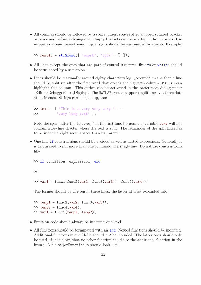
• All commas should be followed by a space. Insert spaces after an open squared bracketor brace and before a closing one. Empty brackets can be written without spaces. Useno spaces around parentheses. Equal signs should be surrounded by spaces. Example:

>> result = str2func([ ’exprb’, ’opts’, [] ]);

• All lines except the ones that are part of control strucures like ifs or whiles shouldbe terminated by a semicolon.

• Lines should be maximally around eighty characters log. „Around“ means that a lineshould be split up after the first word that exeeds the eightieth column. MATLAB canhighlight this column. This option can be activated in the preferences dialog under„Editor/Debugger“ → „Display“. The MATLAB syntax supports split lines via three dotsat their ends. Strings can be split up, too:

>> text = [ ’This is a very very very ’ ...

>> ’very long text’ ];

Note the space after the last „very“ in the first line, because the variable text will notcontain a newline chacter where the text is split. The remainder of the split lines hasto be indented eight more spaces than its parent.

• One-line-if constructions should be avoided as well as nested expressions. Generally itis dicouraged to put more than one command in a single line. Do not use constructionslike:

>> if condition, expression, end

or

>> var1 = func1(func2(var2, func3(var3)), func4(var4));

The former should be written in three lines, the latter at least expanded into

>> temp1 = func2(var2, func3(var3));

>> temp2 = func4(var4);

>> var1 = func1(temp1, temp2);

• Function code should always be indented one level.

• All functions should be terminated with an end. Nested functions should be indented.Additional functions in one M-file should not be intended. The latter ones should onlybe used, if it is clear, that no other function could use the additional function in thefuture. A file majorFunction.m should look like:

33

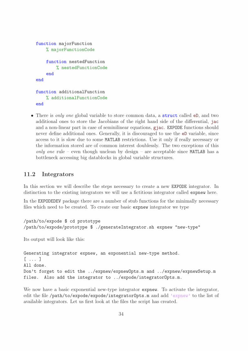
function majorFunction

% majorFunctionCode

function nestedFunction

% nestedFunctionCode

end

end

function additionalFunction

% additionalFunctionCode

end

• There is only one global variable to store common data, a struct called eD, and twoadditional ones to store the Jacobians of the right hand side of the differential, jacand a non-linear part in case of seminilinear equations, gjac. EXPODE functions shouldnever define additional ones. Generally, it is discouraged to use the eD variable, sinceaccess to it is slow due to some MATLAB restrictions. Use it only if really necessary orthe information stored are of common interest doublessly. The two exceptions of thisonly one rule – even though unclean by design – are acceptable since MATLAB has abottleneck accessing big datablocks in global variable structures.

11.2 Integrators

In this section we will describe the steps necessary to create a new EXPODE integrator. Indistinction to the existing integrators we will use a fictitious integrator called expnew here.

In the EXPODEDEV package there are a number of stub functions for the minimally necessaryfiles which need to be created. To create our basic expnew integrator we type

/path/to/expode $ cd prototype

/path/to/expode/prototype $ ./generateIntegrator.sh expnew "new-type"

Its output will look like this:

Generating integrator expnew, an exponential new-type method.

[ ... ]

All done.

Don’t forget to edit the ../expnew/expnewOpts.m and ../expnew/expnewSetup.m

files. Also add the integrator to ../expode/integratorOpts.m.

We now have a basic exponential new-type integrator expnew. To activate the integrator,edit the file /path/to/expode/expode/integratorOpts.m and add ’expnew’ to the list ofavailable integrators. Let us first look at the files the script has created.

34

In the /path/to/expode directory we got the new files expnew.m, the integrator command,expmsset.m, the options setter and expnewinfo.m, the info command. These files are alreadyready to use, as they only wrap already existing EXPODE functions. These wrappers willbe adapted by generateIntegrator.sh to give the correct information to their wrappedfunctions. The script gives us a hint where to start our work. All necessary information forthe integration process have to contained in the two functions in /path/to/expode/expnew,expnewSetup.m and expnewOpts.m. The latter one will be discussed in the next sectionwhere we handle options.

The expnewSetup.m has to feed the expode in its startup phase where it will be called thefollowing way:

function [ o, nv, solverSetup, solverStep, order, errorOrder, multiStep, ...

semilin, denseOutputGenerator ] = expnewSetup(o, nv);

The parameters o and nv contain the options provided by the user and the numeric valuesof the list-type options, see sections 11.3 and 11.4 for details. In case o or nv need to bechanged by the setup routine, they will be returned again. The arguments solverSetup andsolverStep will be discussed below in more detail. Next we have order and errorOrder

which contain the order of the integrator – needed for the user – and the order of theerror estimator – needed for the step size selection – respectively. Futhermore multiStep

counts the number of old time steps to use to approximate the solution at the next step,semilin indicates, wheter this integrator is built for semilinear problem, expode evaluatesthe linear part once at the beginning instead of evaluating the Jacobian at each time step.denseOutputGenerator is a function handle to the dense output generating function. If theintegrator has no specific one, this can be empty.

Additionally to these return arguments, the integrator has to set the eD.int.jobFunctionsfield. It has to be a cell array of function handles to the scalar, vectorized versions of thematrix functions, that need to be evaluated. The order of the elements has to correspond tothe order of the job coefficients that are passed to the matrix function evaluator, see section10 for reference.

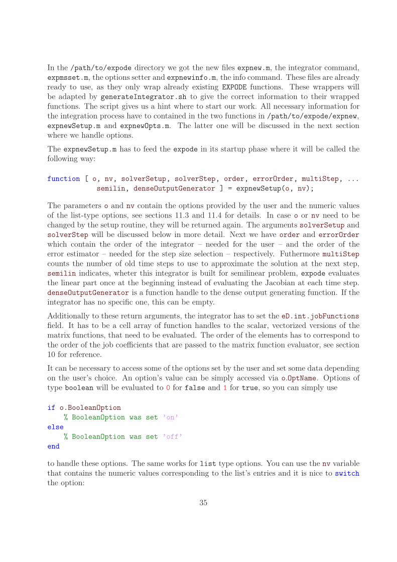
It can be necessary to access some of the options set by the user and set some data dependingon the user’s choice. An option’s value can be simply accessed via o.OptName. Options oftype boolean will be evaluated to 0 for false and 1 for true, so you can simply use

if o.BooleanOption

% BooleanOption was set ’on’

else

% BooleanOption was set ’off’

end

to handle these options. The same works for list type options. You can use the nv variablethat contains the numeric values corresponding to the list’s entries and it is nice to switch

the option:

35

switch o.List

case nv.List.value1

% List was set ’value1’

case nv.List.value2

% List was set ’value2’

case nv.List.value3

% List was set ’value3’

end

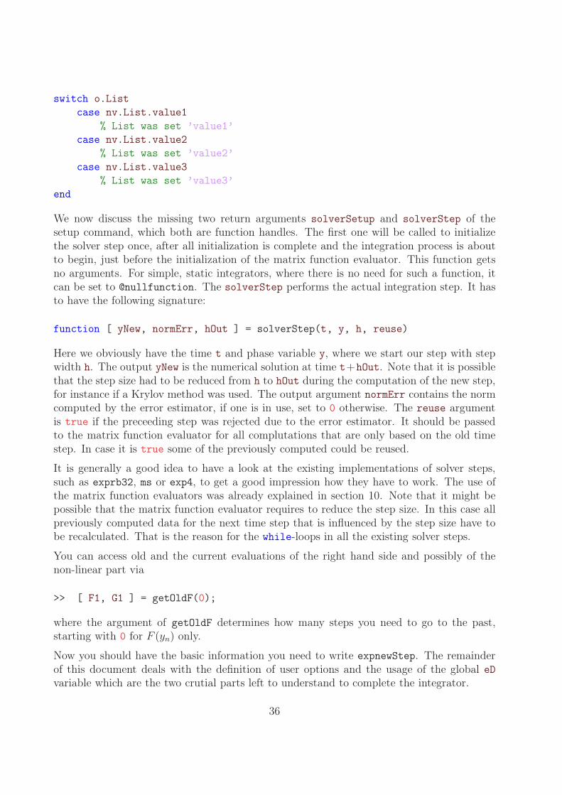
We now discuss the missing two return arguments solverSetup and solverStep of thesetup command, which both are function handles. The first one will be called to initializethe solver step once, after all initialization is complete and the integration process is aboutto begin, just before the initialization of the matrix function evaluator. This function getsno arguments. For simple, static integrators, where there is no need for such a function, itcan be set to @nullfunction. The solverStep performs the actual integration step. It hasto have the following signature:

function [ yNew, normErr, hOut ] = solverStep(t, y, h, reuse)

Here we obviously have the time t and phase variable y, where we start our step with stepwidth h. The output yNew is the numerical solution at time t+hOut. Note that it is possiblethat the step size had to be reduced from h to hOut during the computation of the new step,for instance if a Krylov method was used. The output argument normErr contains the normcomputed by the error estimator, if one is in use, set to 0 otherwise. The reuse argumentis true if the preceeding step was rejected due to the error estimator. It should be passedto the matrix function evaluator for all complutations that are only based on the old timestep. In case it is true some of the previously computed could be reused.

It is generally a good idea to have a look at the existing implementations of solver steps,such as exprb32, ms or exp4, to get a good impression how they have to work. The use ofthe matrix function evaluators was already explained in section 10. Note that it might bepossible that the matrix function evaluator requires to reduce the step size. In this case allpreviously computed data for the next time step that is influenced by the step size have tobe recalculated. That is the reason for the while-loops in all the existing solver steps.

You can access old and the current evaluations of the right hand side and possibly of thenon-linear part via

>> [ F1, G1 ] = getOldF(0);

where the argument of getOldF determines how many steps you need to go to the past,starting with 0 for F (yn) only.

Now you should have the basic information you need to write expnewStep. The remainderof this document deals with the definition of user options and the usage of the global eDvariable which are the two crutial parts left to understand to complete the integrator.

36

11.3 Options

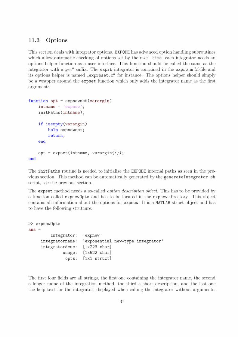
This section deals with integrator options. EXPODE has advanced option handling subroutineswhich allow automatic checking of options set by the user. First, each integrator needs anoptions helper function as a user interface. This function should be called the same as theintegrator with a „set“ suffix. The exprb integrator is contained in the exprb.m M-file andits options helper is named „exprbset.m“ for instance. The options helper should simplybe a wrapper around the expset function which only adds the integrator name as the firstargument:

function opt = expnewset(varargin)

intname = ’expnew’;

initPaths(intname);

if isempty(varargin)

help expnewset;

return;

end

opt = expset(intname, varargin{:});

end

The initPaths routine is needed to initialize the EXPODE internal paths as seen in the pre-vious section. This method can be automatically generated by the generateIntegrator.shscript, see the previous section.

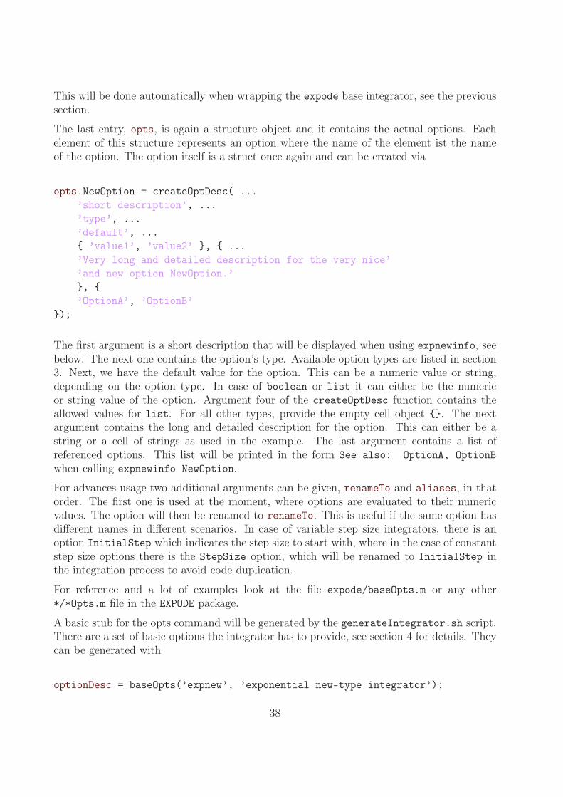
The expset method needs a so-called option description object. This has to be provided bya function called expnewOpts and has to be located in the expnew directory. This objectcontains all information about the options for expnew. It is a MATLAB struct object and hasto have the following strutcure:

>> expnewOpts

ans =

integrator: ’expnew’

integratorname: ’exponential new-type integrator’

integratordesc: [1x223 char]

usage: [1x522 char]

opts: [1x1 struct]

The first four fields are all strings, the first one containing the integrator name, the seconda longer name of the integration method, the third a short description, and the last onethe help text for the integrator, displayed when calling the integrator without arguments.

37

This will be done automatically when wrapping the expode base integrator, see the previoussection.

The last entry, opts, is again a structure object and it contains the actual options. Eachelement of this structure represents an option where the name of the element ist the nameof the option. The option itself is a struct once again and can be created via

opts.NewOption = createOptDesc( ...

’short description’, ...

’type’, ...

’default’, ...

{ ’value1’, ’value2’ }, { ...

’Very long and detailed description for the very nice’

’and new option NewOption.’

}, {

’OptionA’, ’OptionB’

});

The first argument is a short description that will be displayed when using expnewinfo, seebelow. The next one contains the option’s type. Available option types are listed in section3. Next, we have the default value for the option. This can be a numeric value or string,depending on the option type. In case of boolean or list it can either be the numericor string value of the option. Argument four of the createOptDesc function contains theallowed values for list. For all other types, provide the empty cell object {}. The nextargument contains the long and detailed description for the option. This can either be astring or a cell of strings as used in the example. The last argument contains a list ofreferenced options. This list will be printed in the form See also: OptionA, OptionB

when calling expnewinfo NewOption.

For advances usage two additional arguments can be given, renameTo and aliases, in thatorder. The first one is used at the moment, where options are evaluated to their numericvalues. The option will then be renamed to renameTo. This is useful if the same option hasdifferent names in different scenarios. In case of variable step size integrators, there is anoption InitialStep which indicates the step size to start with, where in the case of constantstep size options there is the StepSize option, which will be renamed to InitialStep inthe integration process to avoid code duplication.

For reference and a lot of examples look at the file expode/baseOpts.m or any other*/*Opts.m file in the EXPODE package.

A basic stub for the opts command will be generated by the generateIntegrator.sh script.There are a set of basic options the integrator has to provide, see section 4 for details. Theycan be generated with

optionDesc = baseOpts(’expnew’, ’exponential new-type integrator’);

38

This line of expnewOpts.m is part of the stub and doesn’t need to be adjusted. These basicoptions have to be extended either for use in semilinear integrators or linearized integratorsand for constant or variable step size integrators. The two code lines responsible for this are

optionDesc = linearizationOpts(optionDesc);

optionDesc = varStepOpts(optionDesc);

Use semilinOpts instead of linearizationOpts for semilinear integrators, constStepOptsinstead of varStepOpts for constant step size integration. Using constStepOpts automati-cally switches off the step size estimator.

Another function that needs to be provided for each integrator is the info command. Thisis a wrapper around optInfo similar to the options setter. It will print information on theintegrator. The information will be extracted from the option description object describedabove. Here is its basic structure:

function expnewinfo(optName)

if nargin < 1

optname = ’’;

end

optInfo(’expnew’, optName);

end

Like the set, opts and the integrator command this file will be generated by the scriptgenerateIntegrator.sh.

11.4 The Global eD Variable

This section deals with the main global variable eD. Except for jac and jacv this is theonly global variable used throughout EXPODE (see the coding conventions above). Since ithas such basic relevance it will be discussed in detail here. It is a structure object containingseveral different types of information. After an integrator call, here exprb as an example, itcontains the following fields if the ClearInternalData is set to ’off’:

>> eD

eD =

integrator: ’exprb’

ODE: [1x1 struct]

int: [1x1 struct]

log: [1x1 struct]

evals: [1x1 struct]

functions: [1x1 struct]

39

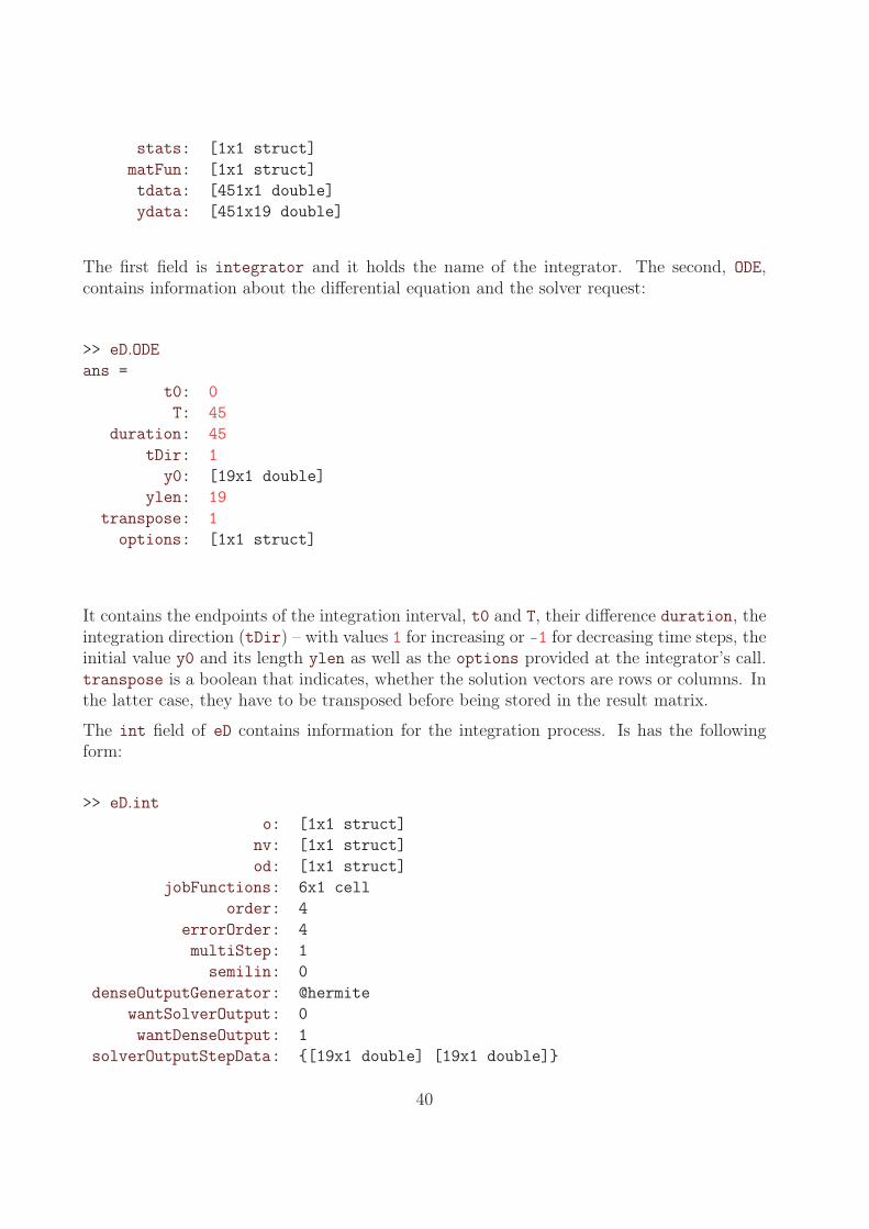
stats: [1x1 struct]

matFun: [1x1 struct]

tdata: [451x1 double]

ydata: [451x19 double]

The first field is integrator and it holds the name of the integrator. The second, ODE,contains information about the differential equation and the solver request:

>> eD.ODEans =

t0: 0

T: 45

duration: 45

tDir: 1

y0: [19x1 double]

ylen: 19

transpose: 1

options: [1x1 struct]

It contains the endpoints of the integration interval, t0 and T, their difference duration, theintegration direction (tDir) – with values 1 for increasing or -1 for decreasing time steps, theinitial value y0 and its length ylen as well as the options provided at the integrator’s call.transpose is a boolean that indicates, whether the solution vectors are rows or columns. Inthe latter case, they have to be transposed before being stored in the result matrix.

The int field of eD contains information for the integration process. Is has the followingform:

>> eD.into: [1x1 struct]

nv: [1x1 struct]

od: [1x1 struct]

jobFunctions: 6x1 cell

order: 4

errorOrder: 4

multiStep: 1

semilin: 0

denseOutputGenerator: @hermite

wantSolverOutput: 0

wantDenseOutput: 1

solverOutputStepData: {[19x1 double] [19x1 double]}

40

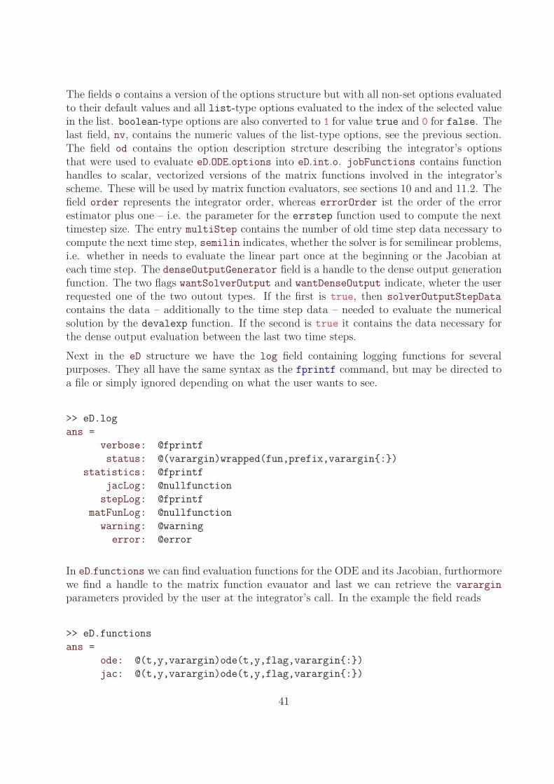
The fields o contains a version of the options structure but with all non-set options evaluatedto their default values and all list-type options evaluated to the index of the selected valuein the list. boolean-type options are also converted to 1 for value true and 0 for false. Thelast field, nv, contains the numeric values of the list-type options, see the previous section.The field od contains the option description strcture describing the integrator’s optionsthat were used to evaluate eD.ODE.options into eD.int.o. jobFunctions contains functionhandles to scalar, vectorized versions of the matrix functions involved in the integrator’sscheme. These will be used by matrix function evaluators, see sections 10 and and 11.2. Thefield order represents the integrator order, whereas errorOrder ist the order of the errorestimator plus one – i.e. the parameter for the errstep function used to compute the nexttimestep size. The entry multiStep contains the number of old time step data necessary tocompute the next time step, semilin indicates, whether the solver is for semilinear problems,i.e. whether in needs to evaluate the linear part once at the beginning or the Jacobian ateach time step. The denseOutputGenerator field is a handle to the dense output generationfunction. The two flags wantSolverOutput and wantDenseOutput indicate, wheter the userrequested one of the two outout types. If the first is true, then solverOutputStepData

contains the data – additionally to the time step data – needed to evaluate the numericalsolution by the devalexp function. If the second is true it contains the data necessary forthe dense output evaluation between the last two time steps.

Next in the eD structure we have the log field containing logging functions for severalpurposes. They all have the same syntax as the fprintf command, but may be directed toa file or simply ignored depending on what the user wants to see.

>> eD.log

ans =

verbose: @fprintf

status: @(varargin)wrapped(fun,prefix,varargin{:})

statistics: @fprintf

jacLog: @nullfunction

stepLog: @fprintf

matFunLog: @nullfunction

warning: @warning

error: @error

In eD.functions we can find evaluation functions for the ODE and its Jacobian, furthormorewe find a handle to the matrix function evauator and last we can retrieve the varargin

parameters provided by the user at the integrator’s call. In the example the field reads

>> eD.functions

ans =

ode: @(t,y,varargin)ode(t,y,flag,varargin{:})

jac: @(t,y,varargin)ode(t,y,flag,varargin{:})

41

matFunV: @matFunKrylov

varargin: {}

The stats field in eD contains statistical data collected over the whole integration process.It has a subfield matFun which contains data gathered by the matrix function evaluators.

The fields tdata and ydata contain the data of the numerical solution. This is what theintegrator returns to the user.

Most of this data will be cleaned before the integration ends. If you want to preserve thedata for testing, set the option ClearInternalData to ’off’.

11.5 Deploying EXPODE

The previous subsection concludes the basic information needed to write new integrators.Additional help can be found using MATLAB’s help command on the EXPODE functions. Allshould be documented well both helptext and code wise. In this subsection you will findsome advices for deployment of your newly created integrator.

The EXPODEDEV package contains a unit testing framework. Before packaging the new releaseit is highly recommended that you run at least the existing tests to make sure that you didn’tintroduce any regression to the previous release. This is done by

>> cd unitTests;

>> runAllTests;

If all goes well you should see a message like

Expode unit tests framework finished.

Totally ran 593 tests, out of where 593 finished successful and 0 failed.

Overall testing time: 00:01:37.

Additionally you should write new unit tests for you new components und run them. Testshave to be located in the unitTests/tests directory. The testing framework clears allglobal variables and restores MATLAB’s default path before calling the actual test. Only oneglobal variable for the testing data will be created, the test itself does not have to use it,though, there are helper functions for it. The test’s working directory is unitTests/tests.You will need to call an intialization routine to tell the framework what you want to test.The next thing you need to do is add the path to your tested functions.

startTest(’optionDesc’);

addpath ../../expode;

Now you can write your testing code. You may need set some values in the global eD variable.After you are done, use

42

finishTest(success);

to report the result, where success is a boolean containing your result. Running this specifictest is done via

>> runTest testname;

run from the unitTests directory again, where testname.m is the name of the m-file. Notethat you can include more that one test into one file, you just have to separate them bystartTest and finishTest. The runTest routine can also run multiple tests in a row, justgive more testnames separated by a space.

Now that you finished testing you new integrator, it is time to release it. In EXPODEDEV youwill find a script, createRelease.sh to do that. You have to add the integrator to the intsvariable. This will automatically include the integrator m-file, the options helper, the infocommand and the integrator’s directory. If you have additional files, you have to add it tothe apropiate variable in the script. This should usually not be the case, since all methodsthat are only used by your new integrator should be in its own directory. Now you can call

/path/to/expode $ ./createRelease.sh 1.1

to create a package for EXPODE, version 1.1. To generate a EXPODEDEV package, call

/path/to/expode $ ./createRelease.sh 1.1-dev -d

which will result in version 1.1-dev with the additional functions described at the beginningof this section.

43

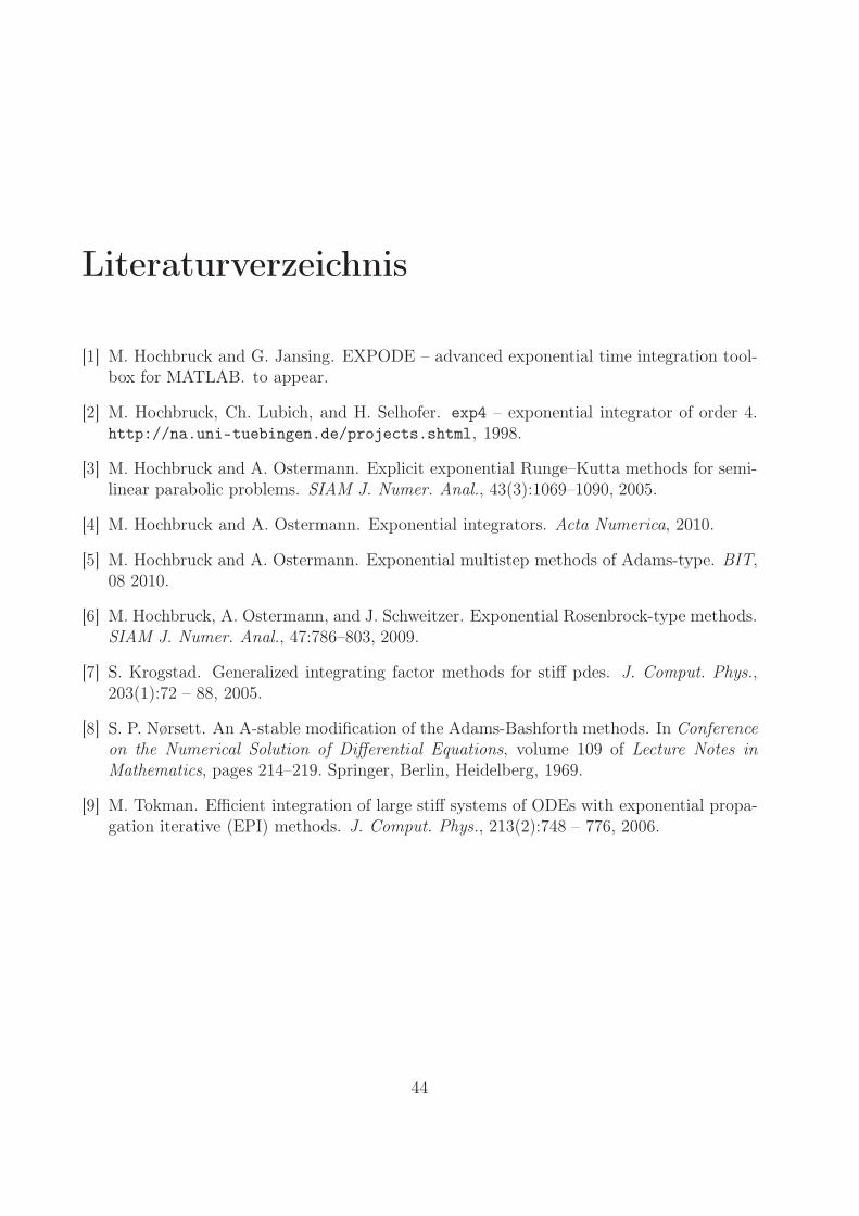
Literaturverzeichnis

[1] M. Hochbruck and G. Jansing. EXPODE – advanced exponential time integration tool-box for MATLAB. to appear.

[2] M. Hochbruck, Ch. Lubich, and H. Selhofer. exp4 – exponential integrator of order 4.http://na.uni-tuebingen.de/projects.shtml, 1998.

[3] M. Hochbruck and A. Ostermann. Explicit exponential Runge–Kutta methods for semi-linear parabolic problems. SIAM J. Numer. Anal., 43(3):1069–1090, 2005.

[4] M. Hochbruck and A. Ostermann. Exponential integrators. Acta Numerica, 2010.

[5] M. Hochbruck and A. Ostermann. Exponential multistep methods of Adams-type. BIT,08 2010.

[6] M. Hochbruck, A. Ostermann, and J. Schweitzer. Exponential Rosenbrock-type methods.SIAM J. Numer. Anal., 47:786–803, 2009.

[7] S. Krogstad. Generalized integrating factor methods for stiff pdes. J. Comput. Phys.,203(1):72 – 88, 2005.

[8] S. P. Nørsett. An A-stable modification of the Adams-Bashforth methods. In Conferenceon the Numerical Solution of Differential Equations, volume 109 of Lecture Notes inMathematics, pages 214–219. Springer, Berlin, Heidelberg, 1969.

[9] M. Tokman. Efficient integration of large stiff systems of ODEs with exponential propa-gation iterative (EPI) methods. J. Comput. Phys., 213(2):748 – 776, 2006.

44