Explosives Detection Technology Barringer Instruments … · summary of the test results for Barringer Instruments’ GC-IONSCAN™. This verification was conducted jointly with the

United States Office of Research and EPA/600/R-00/046 Environmental Protection Development March 2000 Agency Washington, D.C. 20460

Environmental Technology Verification Report

Explosives Detection Technology

Barringer Instruments GC-IONSCAN™

Oak Ridge National Laboratory

THE ENVIRONMENTAL TECHNOLOGY VERIFICATION

Oak Ridge National Laboratory

PROGRAM

Joint Verification Statement

TECHNOLOGY TYPE: EXPLOSIVES DETECTION

APPLICATION: MEASUREMENT OF EXPLOSIVES IN CONTAMINATED SOIL AND WATER

TECHNOLOGY NAME: GC-IONSCAN™

COMPANY: Barringer Instruments

ADDRESS: 30 Technology Drive PHONE: (908) 222-9100Warren, NJ 07059 FAX: (908) 222-1557

WEB SITE: www.barringer.com EMAIL: [email protected]

The U.S. Environmental Protection Agency (EPA) has created the Environmental Technology Verification Program (ETV) to facilitate the deployment of innovative or improved environmental technologies through performance verification and dissemination of information. The goal of the ETV Program is to further environmental protection by substantially accelerating the acceptance and use of improved and cost-effective technologies. ETV seeks to achieve this goal by providing high quality, peer reviewed data on technology performance to those involved in the design, distribution, financing, permitting, purchase, and use of environmental technologies.

ETV works in partnership with recognized standards and testing organizations, stakeholder groups consisting of regulators, buyers, and vendor organizations, with the full participation of individual technology developers. The program evaluates the performance of innovative technologies by developing test plans that are responsive to the needs of stakeholders, conducting field or laboratory tests (as appropriate), collecting and analyzing data, and preparing peer-reviewed reports. All evaluations are conducted in accordance with rigorous quality assurance protocols to ensure that data of known and adequate quality are generated and that the results are defensible.

The Department of Defense (DoD) has a similar verification program known as the Environmental Security Technology Certification Program (ESTCP). The purpose of ESTCP is to demonstrate and validate the most promising innovative technologies that target DoD’s most urgent environmental needs and are projected to pay back the investment within 5 years through cost savings and improved efficiencies. ESTCP demonstrations are typically conducted under operational field conditions at DoD facilities. The

EPA-VS-SCM-45 The accompanying notice is an integral part of this verification statement. March 2000

demonstrations are intended to generate supporting cost and performance data for acceptance or validation of the technology. The goal is to transition mature environmental science and technology projects through the demonstration/ validation phase, enabling promising technologies to receive regulatory and end user acceptance in order to be fielded and commercialized more rapidly.

The Oak Ridge National Laboratory (ORNL) is one of the verification organizations operating under the Site Characterization and Monitoring Technologies (SCMT) program. SCMT, which is administered by EPA’s National Exposure Research Laboratory, is one of 12 technology areas under ETV. In this demonstration, ORNL evaluated the performance of explosives detection technologies. This verification statement provides a summary of the test results for Barringer Instruments’ GC-IONSCAN™. This verification was conducted jointly with the Department of Defense’s (DoD’s) Environmental Security Technology Certification Program (ESTCP).

DEMONSTRATION DESCRIPTION This demonstration was designed to evaluate technologies that detect and measure explosives in soil and water. The demonstration was conducted at ORNL in Oak Ridge, Tennessee, from August 23 through September 1, 1999. Spiked samples of known concentration were used to assess the accuracy of the technology. Environmentally contaminated soil samples, collected from DoD sites in California, Louisiana, Iowa, and Tennessee and ranging in concentration from 0 to approximately 90,000 mg/kg, were used to assess several performance characteristics. Explosives-contaminated water samples from Tennessee, Oregon, and Louisiana with concentrations ranging from 0 to 25,000 mg/L also were analyzed. The primary constituents in the samples were 2,4,6-trinitrotoluene (TNT); isomeric dinitrotoluene (DNT), including both 2,4-dinitrotoluene and 2,6-dinitrotoluene; hexahydro-1,3,5-trinitro-1,3,5-triazine (RDX); and octahydro-1,3,5,7tetranitro-1,3,5,7-tetrazocine (HMX). The results of the soil and water analyses conducted under field conditions by the GC-IONSCAN were compared with results from reference laboratory analyses of homogenous replicate samples determined using EPA SW-846 Method 8330. Details of the demonstration, including a data summary and discussion of results, may be found in the report entitled Environmental Technology Verification Report: Explosives Detection Technology — Barringer Instruments, GC-IONSCAN™, EPA 600-R-00/046.

TECHNOLOGY DESCRIPTION The GC-IONSCAN is a fully transportable field-screening instrument that combines the rapid analysis time of ion mobility spectrometry (IMS) with the separation ability of gas chromatography (GC). The instrument can be operated in IONSCAN mode or in GC-IONSCAN mode to detect explosives. The user can switch between the two modes in less than 30 s through the instrument control panel. In the IONSCAN mode, samples are deposited on a Teflon filter and thermally desorbed directly to the IMS, permitting the quick screening analysis of explosives residues in 6 to 8 s. In the GC-IONSCAN mode, extracts are directly injected onto the GC column and analysis occurs within 1 to 3 minutes, depending on the type of explosive. The use of the IONSCAN mode permits rapid prescreening of samples with identification of the major constituents of the sample and semiquantitative analysis, while the GC-IONSCAN mode permits full characterization and quantitative analysis of the sample. This technology is capable of reporting quantitative data for all of the Method 8330 analytes. The performance assessment described here is only for TNT and RDX because a limited amount of data was available for evaluation of the other analytes. Reporting limits for the GC-IONSCAN ranged from 0.3 to 10 mg/kg for soil and 25 to 1950 mg/L for water.


VERIFICATION OF PERFORMANCE The following performance characteristics of the GC-IONSCAN were observed:

Precision: For the soil samples, the mean relative standard deviations (RSDs) for RDX and TNT were 54% and 51%, respectively. For water samples, the RSDs were significantly lower, at 20% and 26%, respectively.

Accuracy: For the soil samples, the median percent recoveries for RDX and TNT were 55% and 136%, respectively. The results were generally biased low for RDX and biased high for TNT. For water samples, only a few of the RDX and TNT results were reported above the reporting limits in the spiked samples. The recoveries were significantly lower, with the highest recovery at 46%, indicating that the water results were biased low for both analytes.

False positive/false negative results: Of the 20 blank soils, Barringer reported RDX in one sample (5% false positives) and TNT in five samples (25% false positives). No false positives were reported for RDX and TNT in the 20 blank water samples. False positive and false negative results were also determined by comparing the GC-IONSCAN result to the reference laboratory result for the environmental and spiked samples (e.g., whether the GC-IONSCAN reports a result as a nondetect that the reference laboratory reported as a detection, and vice versa). For the soils, 3% of the RDX results and none of the TNT results were reported as false positives relative to the reference laboratory results. Significantly more samples were reported as nondetects by Barringer (i.e., false negatives) when the laboratory reported a detection (2% for RDX and 13% for TNT). Similar results were observed for water, where 2% of the TNT results and none of the RDX results were false positives, and a higher percentage (39% of the RDX results and 21% of the TNT results) were false negatives.

Completeness: The GC-IONSCAN generated results for all 108 soil samples and all 176 water samples, for a completeness of 100%.

Comparability: A one-to-one sample comparison of the GC-IONSCAN results and the reference laboratory results was performed for all samples (spiked and environmental) that were reported as detects. The correlation coefficient (r) for the comparison of the entire soil data set for TNT was 0.88 (slope (m) = 4.82). When comparability was assessed for specific concentration ranges, the r value did not change dramatically for TNT, ranging from 0.71 to 0.85 depending on the concentrations selected. RDX correlation with the reference laboratory for soil was similar (r values near 0.80), except for concentrations greater than 1,000 mg/kg, where the correlation was lower (r = 0.28, m = 0.14). For the water samples, comparability with the reference laboratory results for TNT was much lower than the soil comparison (r = 0.53). For RDX, the correlation was much higher, at 0.95. Although the correlation was high, the slope of the linear regression line was 0.08, indicating that the GC-IONSCAN RDX results were biased low (see Accuracy).

Sample Throughput: Throughput was approximately three samples per hour for soil and eight samples per hour for water. This rate was accomplished by two operators and included sample preparation and analysis.

Ease of Use: Users unfamiliar with ion mobility spectrometry would require approximately two days of training to operate the GC-IONSCAN. Training is provided by Barringer Instruments. No particular level of educational training is required for the operator, but knowledge of chromatographic techniques would be advantageous. Overall Evaluation: The overall performance of the GC-IONSCAN for the analysis of RDX and TNT was characterized as precise and biased low (both analytes) for water analyses, and imprecise and biased (low for


RDX and high for TNT) for soil analyses. As with any technology selection, the user must determine if this technology is appropriate for the application and the project’s data quality objectives. For more information on this and other verified technologies, visit the ETV web site at http://www.epa.gov/etv .

Gary J. Foley, Ph.D. David E. Reichle, Ph.D. Director, National Exposure Research Laboratory Associate Laboratory Director Office of Research and Development Oak Ridge National Laboratory

Jeffrey Marqusee, Ph.D. Department of Defense Director, Environmental Security Technology Certification Program

NOTICE: EPA and ESTCP verifications are based on evaluations of technology performance under specific, predetermined criteria and appropriate quality assurance procedures. EPA, ESTCP, and ORNL make no expressed or implied warranties as to the performance of the technology and do not certify that a technology will always operate as verified. The end user is solely responsible for complying with any and all applicable federal, state, and


http://www.epa.gov/etv

EPA/600/R-XX/YYY March 2000

Environmental Technology Verification Report

Explosives Detection Technology

Barringer Instruments GC-IONSCAN™

By

Amy B. DindalCharles K. Bayne, Ph.D.Roger A. Jenkins, Ph.D.

Oak Ridge National LaboratoryOak Ridge Tennessee 37831-6120

Eric N. KoglinU.S. Environmental Protection Agency

Environmental Sciences DivisionNational Exposure Research Laboratory

Las Vegas, Nevada 89193-3478

This demonstration was conducted in cooperation with theU.S. Department of Defense

Environmental Security Technology Certification Program

Notice

The U.S. Environmental Protection Agency (EPA), through its Office of Research and Development (ORD), and the U.S. Department of Defense’s Environmental Security Technology Certification Program (ESTCP) Program, funded and managed, through Interagency Agreement No. DW89937854 with Oak Ridge National Laboratory, the verification effort described herein. This report has been peer and administratively reviewed and has been approved for publication as an EPA document. Mention of trade names or commercial products does not constitute endorsement or recommendation for use of a specific product.

ii

Table of Contents

List of Figures . . . . . . . . . . . . . . . . . . . . . . . . . . . . . . . . . . . . . . . . . . . . . . . . . . . . . . . . . . . . . . viList of Tables . . . . . . . . . . . . . . . . . . . . . . . . . . . . . . . . . . . . . . . . . . . . . . . . . . . . . . . . . . . . . . . viiiAcknowledgments . . . . . . . . . . . . . . . . . . . . . . . . . . . . . . . . . . . . . . . . . . . . . . . . . . . . . . . . . . . . xList of Abbreviations and Acronyms . . . . . . . . . . . . . . . . . . . . . . . . . . . . . . . . . . . . . . . . . . . . . . xii

1 INTRODUCTION . . . . . . . . . . . . . . . . . . . . . . . . . . . . . . . . . . . . . . . . . . . . . . . . . . . . . . . . . . . 1

2 TECHNOLOGY DESCRIPTION . . . . . . . . . . . . . . . . . . . . . . . . . . . . . . . . . . . . . . . . . . . . . . . . 3Technology Overview . . . . . . . . . . . . . . . . . . . . . . . . . . . . . . . . . . . . . . . . . . . . . . . . . . . . . . . . . 3Sample Preparation . . . . . . . . . . . . . . . . . . . . . . . . . . . . . . . . . . . . . . . . . . . . . . . . . . . . . . . . . . . 4Analytical Determination . . . . . . . . . . . . . . . . . . . . . . . . . . . . . . . . . . . . . . . . . . . . . . . . . . . . . . . 4Instrument Calibration and Quantification of Sample Results . . . . . . . . . . . . . . . . . . . . . . . . . . . . . . 4

3 DEMONSTRATION DESIGN . . . . . . . . . . . . . . . . . . . . . . . . . . . . . . . . . . . . . . . . . . . . . . . . . . 5Objective . . . . . . . . . . . . . . . . . . . . . . . . . . . . . . . . . . . . . . . . . . . . . . . . . . . . . . . . . . . . . . . . . . . 5Demonstration Testing Location and Conditions . . . . . . . . . . . . . . . . . . . . . . . . . . . . . . . . . . . . . . . 5Soil Sample Descriptions . . . . . . . . . . . . . . . . . . . . . . . . . . . . . . . . . . . . . . . . . . . . . . . . . . . . . . . 5

Sources of Samples . . . . . . . . . . . . . . . . . . . . . . . . . . . . . . . . . . . . . . . . . . . . . . . . . . . . . . . . 5Iowa Army Ammunition Plant . . . . . . . . . . . . . . . . . . . . . . . . . . . . . . . . . . . . . . . . . . . . . 5Louisiana Army Ammunition Plant . . . . . . . . . . . . . . . . . . . . . . . . . . . . . . . . . . . . . . . . . . 5Milan Army Ammunition Plant . . . . . . . . . . . . . . . . . . . . . . . . . . . . . . . . . . . . . . . . . . . . . 5Volunteer Army Ammunition Plant . . . . . . . . . . . . . . . . . . . . . . . . . . . . . . . . . . . . . . . . . . 5Fort Ord Military Base . . . . . . . . . . . . . . . . . . . . . . . . . . . . . . . . . . . . . . . . . . . . . . . . . . . 6

Performance Evaluation Samples . . . . . . . . . . . . . . . . . . . . . . . . . . . . . . . . . . . . . . . . . . . . . . 6Soil Sample Preparation . . . . . . . . . . . . . . . . . . . . . . . . . . . . . . . . . . . . . . . . . . . . . . . . . . . . . 6

Water Sample Descriptions . . . . . . . . . . . . . . . . . . . . . . . . . . . . . . . . . . . . . . . . . . . . . . . . . . . . . 7Sources of Samples . . . . . . . . . . . . . . . . . . . . . . . . . . . . . . . . . . . . . . . . . . . . . . . . . . . . . . . . 7Performance Evaluation Samples . . . . . . . . . . . . . . . . . . . . . . . . . . . . . . . . . . . . . . . . . . . . . . 7Water Sample Preparation . . . . . . . . . . . . . . . . . . . . . . . . . . . . . . . . . . . . . . . . . . . . . . . . . . . 7

Sample Randomization . . . . . . . . . . . . . . . . . . . . . . . . . . . . . . . . . . . . . . . . . . . . . . . . . . . . . . . . . 7Summary of Experimental Design . . . . . . . . . . . . . . . . . . . . . . . . . . . . . . . . . . . . . . . . . . . . . . . . . 7Description of Performance Factors . . . . . . . . . . . . . . . . . . . . . . . . . . . . . . . . . . . . . . . . . . . . . . . 7

Precision . . . . . . . . . . . . . . . . . . . . . . . . . . . . . . . . . . . . . . . . . . . . . . . . . . . . . . . . . . . . . . . . 8Accuracy . . . . . . . . . . . . . . . . . . . . . . . . . . . . . . . . . . . . . . . . . . . . . . . . . . . . . . . . . . . . . . . 8False Positive/Negative Results . . . . . . . . . . . . . . . . . . . . . . . . . . . . . . . . . . . . . . . . . . . . . . . 8Completeness . . . . . . . . . . . . . . . . . . . . . . . . . . . . . . . . . . . . . . . . . . . . . . . . . . . . . . . . . . . . 8Comparability . . . . . . . . . . . . . . . . . . . . . . . . . . . . . . . . . . . . . . . . . . . . . . . . . . . . . . . . . . . . 8Sample Throughput . . . . . . . . . . . . . . . . . . . . . . . . . . . . . . . . . . . . . . . . . . . . . . . . . . . . . . . . 9Ease of Use . . . . . . . . . . . . . . . . . . . . . . . . . . . . . . . . . . . . . . . . . . . . . . . . . . . . . . . . . . . . . 9Cost . . . . . . . . . . . . . . . . . . . . . . . . . . . . . . . . . . . . . . . . . . . . . . . . . . . . . . . . . . . . . . . . . . . 9Miscellaneous Factors . . . . . . . . . . . . . . . . . . . . . . . . . . . . . . . . . . . . . . . . . . . . . . . . . . . . . . 9

4 REFERENCE LABORATORY ANALYSES . . . . . . . . . . . . . . . . . . . . . . . . . . . . . . . . . . . . . . . 10Reference Laboratory Selection . . . . . . . . . . . . . . . . . . . . . . . . . . . . . . . . . . . . . . . . . . . . . . . . . . 10Reference Laboratory Method . . . . . . . . . . . . . . . . . . . . . . . . . . . . . . . . . . . . . . . . . . . . . . . . . . . 10Reference Laboratory Performance . . . . . . . . . . . . . . . . . . . . . . . . . . . . . . . . . . . . . . . . . . . . . . . 10

iii

5 TECHNOLOGY EVALUATION . . . . . . . . . . . . . . . . . . . . . . . . . . . . . . . . . . . . . . . . . . . . . . . . 13Objective and Approach . . . . . . . . . . . . . . . . . . . . . . . . . . . . . . . . . . . . . . . . . . . . . . . . . . . . . . . . 13Precision . . . . . . . . . . . . . . . . . . . . . . . . . . . . . . . . . . . . . . . . . . . . . . . . . . . . . . . . . . . . . . . . . . . 13Accuracy . . . . . . . . . . . . . . . . . . . . . . . . . . . . . . . . . . . . . . . . . . . . . . . . . . . . . . . . . . . . . . . . . . 13False Positive/False Negative Results . . . . . . . . . . . . . . . . . . . . . . . . . . . . . . . . . . . . . . . . . . . . . . 14Completeness . . . . . . . . . . . . . . . . . . . . . . . . . . . . . . . . . . . . . . . . . . . . . . . . . . . . . . . . . . . . . . . 15Comparability . . . . . . . . . . . . . . . . . . . . . . . . . . . . . . . . . . . . . . . . . . . . . . . . . . . . . . . . . . . . . . . 15Sample Throughput . . . . . . . . . . . . . . . . . . . . . . . . . . . . . . . . . . . . . . . . . . . . . . . . . . . . . . . . . . . 18Ease of Use . . . . . . . . . . . . . . . . . . . . . . . . . . . . . . . . . . . . . . . . . . . . . . . . . . . . . . . . . . . . . . . . 18Cost Assessment . . . . . . . . . . . . . . . . . . . . . . . . . . . . . . . . . . . . . . . . . . . . . . . . . . . . . . . . . . . . . 18

GC-IONSCAN Costs . . . . . . . . . . . . . . . . . . . . . . . . . . . . . . . . . . . . . . . . . . . . . . . . . . . . . . 19Reference Laboratory Costs . . . . . . . . . . . . . . . . . . . . . . . . . . . . . . . . . . . . . . . . . . . . . . . . . . 21Cost Assessment Summary . . . . . . . . . . . . . . . . . . . . . . . . . . . . . . . . . . . . . . . . . . . . . . . . . . 21

Miscellaneous Factors . . . . . . . . . . . . . . . . . . . . . . . . . . . . . . . . . . . . . . . . . . . . . . . . . . . . . . . . . 21Summary of Performance . . . . . . . . . . . . . . . . . . . . . . . . . . . . . . . . . . . . . . . . . . . . . . . . . . . . . . 22

6 TECHNOLOGY UPDATE . . . . . . . . . . . . . . . . . . . . . . . . . . . . . . . . . . . . . . . . . . . . . . . . . . . . . 24Rapid Prescreening of Samples . . . . . . . . . . . . . . . . . . . . . . . . . . . . . . . . . . . . . . . . . . . . . . . . . . . 24Improvements to GC-IONSCAN . . . . . . . . . . . . . . . . . . . . . . . . . . . . . . . . . . . . . . . . . . . . . . . . . 24

7 REFERENCES . . . . . . . . . . . . . . . . . . . . . . . . . . . . . . . . . . . . . . . . . . . . . . . . . . . . . . . . . . . . . . 25

APPENDICES A: GC-IONSCAN Sample Soil Results Compared with Reference Laboratory Results . . . . . . . 27B: GC-IONSCAN Sample Water Results Compared with Reference Laboratory Results . . . . . . 33

iv

List of Figures

1 The GC-IONSCAN . . . . . . . . . . . . . . . . . . . . . . . . . . . . . . . . . . . . . . . . . . . . . . . . . . . . . . . . . . . 32 Comparability of reference laboratory TNT soil results with GC-IONSCAN results for vendor

concentrations less than 500 mg/kg . . . . . . . . . . . . . . . . . . . . . . . . . . . . . . . . . . . . . . . . . . . . . . . . 173 Comparability of reference laboratory RDX water results with GC-IONSCAN results

for all results reported above reporting limits . . . . . . . . . . . . . . . . . . . . . . . . . . . . . . . . . . . . . . . . . 184 Range of percent difference values for TNT in soil and water . . . . . . . . . . . . . . . . . . . . . . . . . . . . 195 Range of percent difference values for RDX in soil and water . . . . . . . . . . . . . . . . . . . . . . . . . . . . 20

vi

1 2 3 4 5 6 7 8 9

List of Tables

Summary of Soil and Water Samples . . . . . . . . . . . . . . . . . . . . . . . . . . . . . . . . . . . . . . . . . . . . . . . 8Summary of the Reference Laboratory Performance for Soil Samples . . . . . . . . . . . . . . . . . . . . . . 11Summary of the Reference Laboratory Performance for Water Samples . . . . . . . . . . . . . . . . . . . . 11Summary of the Reference Laboratory Performance on Blank Samples . . . . . . . . . . . . . . . . . . . . . 12Summary of the GC-IONSCAN Precision . . . . . . . . . . . . . . . . . . . . . . . . . . . . . . . . . . . . . . . . . . . 13Summary of the GC-IONSCAN Accuracy . . . . . . . . . . . . . . . . . . . . . . . . . . . . . . . . . . . . . . . . . . 14Number of GC-IONSCAN Results within Acceptance Ranges for Spiked Soils . . . . . . . . . . . . . . . . 14Summary of GC-IONSCAN False Positives on Blank Soil and Water Samples . . . . . . . . . . . . . . . . 15Summary of the GC-IONSCAN Detect/Nondetect Performance Relative to the Reference Laboratoryresults . . . . . . . . . . . . . . . . . . . . . . . . . . . . . . . . . . . . . . . . . . . . . . . . . . . . . . . . . . . . . . . . . . . . . 15

10 GC-IONSCAN Correlation with Reference Data for Various Vendor Soil Concentration Ranges . . . 1611 GC-IONSCAN Correlation with Reference Data for Various Vendor Water Concentration Ranges . 1612 Estimated analytical costs for explosives-contaminated samples . . . . . . . . . . . . . . . . . . . . . . . . . . . 2213 Performance Summary for the GC-IONSCAN . . . . . . . . . . . . . . . . . . . . . . . . . . . . . . . . . . . . . . . 23

viii

Acknowledgments

The authors wish to acknowledge the support of all those who helped plan and conduct the demonstration, analyze the data, and prepare this report. In particular, we recognize Dr. Thomas Jenkins (U.S. Army, Cold Regions Research and Engineering Laboratory) and Dr. Michael Maskarinec (Oak Ridge National Laboratory) who served as the technical experts for this project. We thank the people who helped us to obtain the samples from the various sites, including Dr. Jenkins, Danny Harrelson (Waterways Experiment Station), Kira Lynch (U.S. Army Corp of Engineers, Seattle District), Larry Stewart (Milan Army Ammunition Plant), Dick Twitchell and Bob Elmore (Volunteer Army Ammunition Plant). For external peer review, we thank Dr. C. L. Grant (Professor Emeritus, University of New Hampshire). For internal peer review, we thank Stacy Barshick of Oak Ridge National Laboratory and Harry Craig of EPA Region 10. The authors also acknowledge the participation of Yin Sun and Tri Le of Barringer Instruments, who performed the analyses during verification testing.

For more information on the Explosives Detection Technology Demonstration contact

Eric N. Koglin Amy B. Dindal Project Technical Leader Technical Lead Environmental Protection Agency Oak Ridge National Laboratory Environmental Sciences Division Chemical and Analytical Sciences Division National Exposure Research Laboratory P.O. Box 2008 P. O. Box 93478 Building 4500S, MS-6120 Las Vegas, Nevada 89193-3478 Oak Ridge, TN 37831- 6120 (702) 798-2432 (865) 574-4863 [email protected] [email protected]

For more information on Barringer Instruments’ GC-IONSCAN contact

Reno DeBono Andy Rudolph, Ph.D.Barringer Instruments GC-IONSCAN Project Manager30 Technology Drive Barringer Research Ltd.Warren, NJ 07059 1730 Aimco Blvd.(908) 222-9100, ext 3017 Mississauga, Ontario L4W 1V1 [email protected] Canada www.barringer.com Phone: (905) 238-8837

Fax: (905) 238-3018 [email protected]

x

mailto:[email protected]



Abbreviations and Acronyms

2-Am-DNT 2-amino-4,6-dinitrotoluene, CAS # 35572-78-2 4-Am-DNT 4-amino-2,6-dinitrotoluene, CAS # 1946-51-0 CRREL U.S. Army Cold Regions Research and Engineering Laboratory 2,4-DNT 2,4-dinitrotoluene, CAS # 121-14-2 2,6-DNT 2,6-dinitrotoluene, CAS # 606-20-2 DNT isomeric dinitrotoluene (includes both 2,4-DNT and 2,6-DNT) DoD U.S. Department of Defense EPA U.S. Environmental Protection Agency ERA Environmental Resource Associates ESTCP Environmental Security Technology Certification Program ETV Environmental Technology Verification Program fn false negative result fp false positive result GC gas chromatography HMX octahydro-1,3,5,7-tetranitro-1,3,5,7-tetrazocine, CAS # 2691-41-0 HPLC high performance liquid chromatography IMS ion mobility spectrometry LAAAP Louisiana Army Ammunition Plant MLAAP Milan Army Ammunition Plant NERL National Exposure Research Laboratory (EPA) ORNL Oak Ridge National Laboratory PE performance evaluation sample QA quality assurance QC quality control RDX hexahydro-1,3,5-trinitro-1,3,5-triazine, CAS # 121-82-4 RSD percent relative standard deviation SCMT Site Characterization and Monitoring Technologies Pilot of ETV SD standard deviation TNB 1,3,5-trinitrobenzene, CAS # 99-35-4 TNT 2,4,6-trinitrotoluene, CAS # 118-96-7 USACE U.S. Army Corps of Engineers

xii

Section 1 — Introduction

The U.S. Environmental Protection Agency (EPA) created the Environmental Technology Verification Program (ETV) to facilitate the deployment of innovative or improved environmental technologies through performance verification and dissemination of information. The goal of the ETV Program is to further environmental protection by substantially accelerating the acceptance and use of improved and cost-effective technologies. ETV seeks to achieve this goal by providing high-quality, peerreviewed data on technology performance to those involved in the design, distribution, financing, permitting, purchase, and use of environmental technologies.

ETV works in partnership with recognized standards and testing organizations and stakeholder groups consisting of regulators, buyers, and vendor organizations, with the full participation of individual technology developers. The program evaluates the performance of innovative technologies by developing verification test plans that are responsive to the needs of stakeholders, conducting field or laboratory tests (as appropriate), collecting and analyzing data, and preparing peer-reviewed reports. All evaluations are conducted in accordance with rigorous quality assurance (QA) protocols to ensure that data of known and adequate quality are generated and that the results are defensible.

ETV is a voluntary program that seeks to provide objective performance information to all of the participants in the environmental marketplace and to assist them in making informed technology decisions. ETV does not rank technologies or compare their performance, label or list technologies as acceptable or unacceptable, seek to determine “best available technology,” or approve or disapprove technologies. The program does not evaluate technologies at the bench or pilot scale and does not conduct or support research. Rather, it conducts and reports on testing designed to describe the performance of technologies under a range of environmental conditions and matrices.

The program now operates 12 pilots covering a broad range of environmental areas. ETV has begun with a 5-year pilot phase (1995–2000) to test a wide range of partner and procedural alternatives in various pilot areas, as well as the true market demand for and response to such a program. In these pilots, EPA utilizes the expertise of partner “verification organizations” to design efficient processes for conducting performance tests of innovative technologies. These expert partners are both public and private organizations, including federal laboratories, states, industry consortia, and private sector entities. Verification organizations oversee and report verification activities based on testing and QA protocols developed with input from all major stakeholder/customer groups associated with the technology area. The verification described in this report was administered by the Site Characterization and Monitoring Technologies (SCMT) Pilot, with Oak Ridge National Laboratory (ORNL) serving as the verification organization. (To learn more about ETV, visit ETV’s Web site at http://www.epa.gov/etv.) The SCMT pilot is administered by EPA’s National Exposure Research Laboratory (NERL), Environmental Sciences Division, in Las Vegas, Nevada.

The Department of Defense (DoD) has a similar verification program known as the Environmental Security Technology Certification Program (ESTCP). The purpose of ESTCP is to demonstrate and validate the most promising innovative technologies that target DoD’s most urgent environmental needs and are projected to pay back the investment within 5 years through cost savings and improved efficiencies. ESTCP responds to (1) concern over the slow pace and cost of remediation of environmentally contaminated sites on military installations, (2) congressional direction to conduct demonstrations specifically focused on new technologies, (3) Executive Order 12856, which requires federal agencies to place high priority on obtaining funding and resources needed for the development of innovative pollution prevention programs and technologies for installations and in acquisitions, and (4) the need to improve defense

1

http://www.epa.gov/etv.)

readiness by reducing the drain on the Department’s operation and maintenance dollars caused by real world commitments such as environmental restoration and waste management. ESTCP demonstrations are typically conducted under operational field conditions at DoD facilities. The demonstrations are intended to generate supporting cost and performance data for acceptance or validation of the technology. The goal is to transition mature environmental science and technology projects through the demonstration/ validation phase, enabling promising technologies to receive regulatory and end user acceptance in order to be fielded and commercialized more rapidly. (To learn more about ESTCP, visit ESTCP’s web site at http://www.estcp.org.)

EPA’s ETV program and DoD’s ESTCP program established a memorandum of agreement in 1999 to work cooperatively with ESTCP on the verification of technologies that are used to improve environmental cleanup and protection at both DOD and non-DOD sites. The verification of field analytical technologies for explosives detection described in this report was conducted jointly by ETV’s SCMT pilot and ESTCP. The verification was conducted at ORNL in Oak Ridge, Tennessee,

from August 23 through September 1, 1999. The performances of two field analytical techniques for explosives were determined under field conditions. Each technology was independently evaluated by comparing field analysis results with those obtained using an approved reference method, EPA SW-846 Method 8330. The demonstration was designed to evaluate the field technology’s ability to detect and measure explosives in soil and water. The primary constituents in the samples were 2,4,6-trinitrotoluene (TNT); isomeric dinitrotoluene (DNT), including both 2,4-dinitrotoluene (2,4-DNT) and 2,6-dinitrotoluene (2,6-DNT); hexahydro-1,3,5-trinitro-1,3,5-triazine (RDX); and octahydro-1,3,5,7-tetranitro-1,3,5,7tetrazocine (HMX). Naturally contaminated environmental soil samples, ranging in concentration from 0 to about 90,000 mg/kg, were collected from DoD sites in California, Louisiana, Iowa, and Tennessee, and were used to assess several performance characteristics. Explosivescontaminated water samples from Tennessee, Oregon, and Louisiana with concentrations ranging from 0 to 25,000 mg/L were also evaluated. This report discusses the performance of Barringer Instruments’ GC-IONSCAN™.

2

http://www.estcp.org.)

Section 2 — Technology Description

In this section, the vendor (with minimal editorial changes by ORNL) provides a description of the technology and the analytical procedure used during the verification testing activities.

Technology Overview The GC-IONSCAN, which weighs approximately 70 lb and is shown in Figure 1, is an on-site analytical instrument combining the rapid analysis time of ion mobility spectrometry (IMS) with the separation capability of gas chromatography (GC). In IMS, ions are generated by atmospheric pressure chemical ionization and drift through a buffer gas under the influence of an electric field. The rate of drift of ions through the field is dependent upon both the physical and electrical properties of the molecules, and can be used to discriminate between compounds based on size-to-charge ratio. In GC, components of complex mixtures are separated by a stationary phase; the separation occurs on the basis of the relative affinity of the compounds for the stationary phase.

The analytical process begins with the eluent entering the IONSCAN inlet. The sample then combines with makeup gas (air filtered with charcoal and Drierite™) doped with reactant, and proceeds

Figure 1. The GC-IONSCAN.

into the ionization region, where the sample is selectively ionized to form ions or ionic clusters of specific mobilities (drift time). The gating grid opens, allowing ions of the correct polarity (negative for explosives) enter the drift region. The ions are then focused and accelerated by the electric field along the drift region of the IMS tube and arrive at the collector electrode (typically 10–20 ms). IMS identifies individual explosives based on the unique ion mobilities (drift time) of specific compounds.

The instrument can be operated in IONSCAN mode or in GC-IONSCAN mode. The user can switch between the two modes in less than 30 s through the instrument control panel. In the IONSCAN mode, samples are deposited on a Teflon filter, allowed to evaporate and then thermally desorbed directly into the IMS, permitting quick screening analysis of explosives residues in 6–8 s. In the GC-IONSCAN mode, extracts are directly injected onto the GC column and analysis occurs within 1–3 min, depending on the type of explosive and the GC column used. The use of the IONSCAN mode permits rapid prescreening of samples, with identification of the major constituents of the sample and semiquantitative analysis, while the GC-IONSCAN mode permits full characterization and quantitative analysis of the sample.

At the time of the demonstration, the cost of purchasing the GC-IONSCAN was $60,000. The kit included a laptop computer, a standard spare kit, a standard maintenance kit, a standard consumables kit, a sampling kit, a swab sampler, IM software, and an operator’s manual; the price also included training at Barringer for up to six people. The kit is supplied in a aluminum carrying case that can also be used to ship the instrument. The instrument can be operated in two modes: explosives detection and drug detection. As with any instrument, the cost on a persample basis would decrease with an increase in the number of analyses performed.

3

Sample Preparation In the demonstration, minimal sample preparation was performed. The preparation of soil samples involved one-step solvent extraction with acetone. Ten milliliters of acetone was added to 2 g of soil in a 20-mL vial. The mixture was shaken in a vortex mixer for 2–3 min. After the solution settled for approximately 1 min, two dilutions using acetone (10and 100-fold) were prepared for each sample from the acetone fraction. If the sample contained high levels of explosives (based on IONSCAN mode analysis), it was further diluted.

The preparation of water samples involved adding 2 mL of sample to 1 g of sodium sulfate in a 20-mL vial and then adding 1 mL of acetone. The mixture was shaken in a vortex mixer for 2–3 min. If the sample was too concentrated, based on the GC-IONSCAN response, the sample was diluted by 1:10 and reanalyzed.

Analytical Determination In GC-IONSCAN mode, a 15-m MXT-1 column (internal diameter of 0.53 mm and film thickness of 1.0 mm), operated in the splitless mode with nitrogen carrier gas, was used for the demonstration sample analyses. The injector port temperature was 260ºC. The oven temperature program was 160ºC; this temperature was held for 60 s and then ramped at a rate of 40ºC /min to 240ºC, for a 180-s analysis time. Analyses not including HMX were performed isothermally at 160ºC, resulting in a 90-s analysis time. A 0.5-m transfer line from the end of the column to the detector was at 195ºC.

For the soil analyses, extracts were screened in the IONSCAN mode. After a 1-mL aliquot of the sample extract was deposited on the Teflon filter, the acetone was allowed to evaporate (taking approximately 15–20 s); then the filter was thermally desorbed. The Barringer team analyzed extracts (for a given sample) in the following order: the 100-fold dilution, the 10-fold dilution, the undiluted extract, and 4 mL of the undiluted extract. If no explosives were detected, a more concentrated extract was analyzed. If no explosives were detected in the 4-mL undiluted

extract, the sample was reported as less than the reporting limit of the GC-IONSCAN. If explosives were detected in the extracts using the IONSCAN mode, the sample was analyzed in the GC-IONSCAN mode.

For the analysis of aqueous samples, no prescreening was performed in the IONSCAN mode. A 2-mL aliquot from the acetone fraction was injected into the heated injector port of the GC-IONSCAN. The sample was either quantified, diluted, and reanalyzed, or reported as a nondetect, as appropriate. The Barringer team elected not to analyze water samples for HMX.

Instrument Calibration and Quantification of Sample Results At the beginning of the day multiple 1-mL injections of a standard containing all of the method analytes were used to deactivate any active sites within the instrument. The standard contained 4 ng/mL for all analytes except as follows: HMX, 20 ng/mL; 2,4-DNT, 20 ng/mL; 2,6-DNT 1,000 ng/mL. The GC-IONSCAN instrument was initially calibrated by use of eight calibration standards, ranging in concentration from 0.5 ng/mL to 10 ng/mL for TNT, RDX, HMX, TNB, 2-amino-4,6-dinitrotoluene (2-Am-DNT), and 4-amino-2,6-dinitrotoluene (4-Am-DNT); from 10 to 100 ng for 2,4-DNT; and from 1000 to 4000 ng for 2,6-DNT. Linear or logarithmic expressions were used to generate the calibration curves. The calibration was checked every 15 samples by analyzing a mid-level standard. If the value was within 30% of the initial calibration value, the calibration was considered still valid. If the response had changed by greater than 30%, the instrument was recalibrated. The concentration of explosives in the sample was calculated by comparing the response in the sample extracts to the calibration curve. Reporting limits ranged from 0.3 to 10 mg/kg for soil and 25 to 1950 mg/L for water, depending on the analyte.

4

Section 3 — Demonstration Design

Objective The purpose of this section is to describe the demonstration design. It is a summary of the technology demonstration plan (ORNL 1999).

Demonstration Testing Location and Conditions The verification of field analytical technologies for explosives was conducted at the ORNL Freels Bend Cabin site, in Oak Ridge, Tennessee. The site is somewhat primitive, with no running water, but the vendors were provided with some shelter (porch overhang) and electrical power. The temperature and relative humidity were monitored during field testing. Over the ten days of testing, the average temperature was 77ºF, and ranged from 60 to 88ºF. The average relative humidity was 67%, and ranged from 35 to 96%.

The samples used in this study were brought to the demonstration testing location for evaluation by the vendors. Explosives-contaminated soils from Army ammunition plants in Iowa, Louisiana, and Tennessee and a former Army base in California (Fort Ord) were used in this verification. In addition, explosives-contaminated water samples were analyzed from DoD sites in Oregon, Louisiana, and Tennessee. Because samples were obtained from multiple DoD sites, the samples represented a reasonable cross section of the population of explosives-contaminated matrices, such that the versatility of the field technology could be evaluated. The vendors had the choice of analyzing either soil or water samples, or both matrices. More specific details about the samples are presented below.

Soil Sample Descriptions The primary constituents in the soil samples were TNT, DNT, RDX, and HMX. The samples also contained trace amounts of 2-amino-4,6dinitrotoluene (2-Am-DNT) and 4-amino-2,6dinitrotoluene (4-Am-DNT), which are degradation products of TNT. The total concentration of explosives ranged from 0 to approximately

90,000 mg/kg. The following sections describe the sites from which the samples were collected.

Sources of Samples Iowa Army Ammunition Plant Currently an active site, the Iowa Army Ammunition Plant was constructed to load, assemble, and pack various conventional ammunition and fusing systems. Current production includes 120-mm tank rounds, warheads for missiles, and mine systems. During the early years of use, the installation used surface impoundments, landfills, and sumps for disposal of industrial wastes containing explosives. The major contaminants in these samples were TNT, RDX, and HMX.

Louisiana Army Ammunition Plant The Louisiana Army Ammunition Plant (LAAAP), near Shreveport, Louisiana, is a government-owned facility that began production in 1942. The facility is currently an Army Reserve plant. Production items at LAAAP have included metal parts for artillery shells; the plant also loads, assembles, and packs artillery shells, mines, rockets, mortar rounds, and demolition blocks. As a result of these activities and the resulting soil and groundwater contamination, EPA placed LAAAP on the National Priorities List of contaminated sites (Superfund) in 1989. The major constituents in the samples from this site were TNT, RDX, and HMX, with trace levels of 1,3,5trinitrobenzene (TNB), DNT, 2-Am-DNT, and 4-Am-DNT.

Milan Army Ammunition Plant Currently active, the Milan Army Ammunition Plant (MLAAP) in Milan, Tennessee, was established in late 1940 as part of the pre–World War II buildup. The facility still has ten ammunition loading, assembly, and packaging lines. Munitions-related wastes have resulted in soil contamination. The primary contaminants in these soils were RDX and TNT.

Volunteer Army Ammunition Plant The Volunteer Army Ammunition Plant, in Chattanooga, Tennessee, was built in 1941 to

5

manufacture TNT and DNT. All production ceased in 1977. Past production practices resulted in significant soil and groundwater contamination. In the samples from this site, concentrations of TNT and DNT ranged from 10 to 90,000 mg/kg, with significantly smaller concentrations of Am-DNT isomers.

Fort Ord Military Base Fort Ord, located near Marina, California, was opened in 1917 as a training and staging facility for infantry troops and was closed as a military installation in 1993. Since then, several nonmilitary uses have been established on the site: California State University at Monterey Bay has opened its doors on former Fort Ord property, the University of California at Santa Cruz has established a new research center there, the Monterey Institute of International Studies will take over the officer’s club and several other buildings, and the post’s airfield was turned over to the city of Marina. The Army still occupies several buildings.

An Army study conducted in 1994 revealed that the impact areas at the inland firing ranges of Fort Ord were contaminated with residues of high explosives (Jenkins, Walsh, and Thorne 1998). Fort Ord is on the National Priorities List of contaminated sites (Superfund), requiring the installation to be characterized and remediated to a condition that does not pose unacceptable risks to public health or the environment. The contaminant present at the highest concentration (as much as 300 mg/kg) was HMX; much lower concentrations of RDX, TNT, 2-Am-DNT, and 4-Am-DNT are present.

Performance Evaluation Samples Spiked soil samples were obtained from Environmental Resource Associates (ERA, Arvada, Colo.). The soil was prepared using ERA’s semivolatile blank soil matrix. This matrix was a 40% clay topsoil that had been dried, sieved, and homogenized. Particle size was 60 mesh and smaller. The samples, also referred to as performance evaluation (PE) samples, contained known levels of TNT and RDX. The concentrations that were evaluated contained 10, 50, 100, 250, and 500 mg/kg of each analyte. Prior to the demonstration, ORNL analyzed the spiked samples to confirm the concentrations. The method used was

a modified Method 8330, similar to the reference laboratory method described in Section 4. For the demonstration, four replicates were prepared at each concentration level.

Blank soil samples were evaluated to determine the technology’s ability to identify samples with no contamination (i.e., to ascertain the false positive error rate). The soil was collected in Monroe County, Tennessee, and was certified by ORNL to be free of contamination prior to verification testing. A reasonable number of blanks (N = 20) was chosen to balance the uncertainty for estimating the false positive error rate and the required number of blank samples to be measured.

Soil Sample Preparation A few weeks prior to the demonstration, all of the soil samples were shipped in plastic Ziplock bags at ambient temperature to ORNL. The samples were stored frozen (<0ºC) prior to preparation. To ensure that the developers and the reference laboratory analyzed comparable samples, the soils were homogenized prior to sample splitting. The process was as follows. The sample was kneaded in the Ziplock bag to break up large clumps. Approximately 1500 g of soil was poured into a Pyrex pan, and debris was removed. The sample was then air-dried overnight. The sample was sieved using a 10-mesh (2-mm particle size) screen and placed in a 1-L widemouthed jar. After thorough mixing with a metal spatula, the sample was quartered. After mixing each quarter, approximately 250 g from each quarter was placed back in the 1-L widemouthed jar, for a total sample amount of approximately 1000 g. Analysis by the ORNL method confirmed sample homogeneity (variability of 20% relative standard deviation or less for replicate measurements). The sample was then split into subsamples for analysis during the demonstration. Each 4-oz sample jar contained approximately 20 g of soil. Four replicate splits of each soil sample were prepared for each participant. The design included a one-to-one pairing of the replicates, such that the vendor and reference lab samples could be directly matched. Three replicate sets of samples were also prepared for archival storage. To ensure that degradation did not occur, the soil samples were frozen (<0ºC) until analysis (Maskarinec et al. 1991).

6

Water Sample Descriptions Sources of Samples Explosives-contaminated water samples from Tennessee, Oregon, and Louisiana were analyzed. The contamination in the water samples ranged in concentration from 0 to about 25,000 mg/L. Water samples were collected from LAAAP, MLAAP, and Volunteer, described in the previous section (see “Sources of Samples”). Water samples were also obtained from Umatilla Chemical Depot, described below.

Umatilla Chemical Depot is located in northeastern Oregon. The mission of the facility recently changed to storage of chemical warfare ammunition. Once the chemicals are destroyed, the installation is scheduled to close. Several environmental sites have been identified for cleanup prior to base closure. One site has explosives-contaminated groundwater; the cleanup identified for this site is to pump and treat the water with granulated activated carbon. The major contaminants in these samples were TNT, RDX, HMX, and TNB. According to a remedial investigation conducted at the site, these samples were not contaminated with any chemical warfare agents.

Performance Evaluation Samples Water samples of known concentration were prepared by the U.S. Army Cold Regions Research and Engineering Laboratory (CRREL) in Hanover, New Hampshire. These samples were used to determine the technology’s accuracy. The concentrations of TNT and RDX in the spiked distilled water samples were 25, 100, 200, 500, and 1000 mg/L for each analyte; four replicates were prepared at each concentration. Prior to the demonstration, ORNL analyzed the spiked samples to confirm the concentrations.

Distilled water obtained from ORNL was used for the blanks. As with the soil samples, 20 blank samples were analyzed.

Water Sample Preparation The water samples were collected in 2.5-gal carboys approximately 7 to 10 days prior to the start of the demonstration and shipped on ice to ORNL. To ensure that degradation did not occur, the samples were stored under refrigeration until analysis (~4ºC)

(Maskarinec et al. 1999). Sample splitting was performed in a small laboratory cold room, which was maintained at 4ºC. To prepare the water sample, a spout was attached to the 2.5-gal carboy, and the water sample was split by filling multiple 250-mL amber glass bottles. As with the soil samples, four replicate splits of each water sample were prepared for each participant, and three sets of samples were also prepared for archival storage.

Sample Randomization The samples were randomized in two stages. First, the order in which the filled jars were distributed was randomized so that the same developer did not always receive the first jar filled for a given sample set. Second, the order of analysis was randomized so that each participant analyzed the same set of samples, but in a different order. Each jar was labeled with a sample number. Replicate samples were assigned unique (but not sequential) sample numbers. Spiked materials and blanks were labeled in the same manner, such that these quality control samples were indistinguishable from other samples. All samples were analyzed blindly by both the developer and the reference laboratory.

Summary of Experimental Design The distribution of samples from the various sites is described in Table 1. A total of 108 soil samples were analyzed, with approximately 60% of the samples being naturally contaminated environmental soils, and the remaining 40% being spikes and blanks. A total of 176 water samples were analyzed, with approximately 75% of the samples being naturally contaminated environmental water, and the remaining 25% being spikes and blanks. Four replicates were analyzed for each sample type. For example, four replicate splits of each of three Fort Ord soils were analyzed, for a total of 12 individual Fort Ord samples.

Description of Performance Factors In Section 5, technology performance is evaluated in terms of precision, accuracy, completeness, and comparability, which are indicators of data quality (EPA 1998). False positive and negative results, sample throughput, and ease of use are also evaluated. Each of these performance characteristics is defined in this section.

7

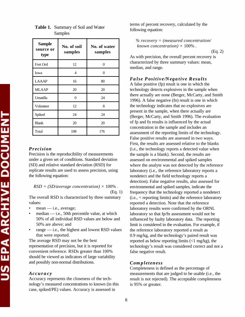
Table 1. Summary of Soil and Water Samples

Sample source or

type

No. of soil samples

No. of water samples

Fort Ord 12 0

Iowa 4 0

LAAAP 16 80

MLAAP 20 20

Umatilla 0 24

Volunteer 12 8

Spiked 24 24

Blank 20 20

Total 108 176

Precision Precision is the reproducibility of measurements under a given set of conditions. Standard deviation (SD) and relative standard deviation (RSD) for replicate results are used to assess precision, using the following equation:

RSD = (SD/average concentration) × 100% . (Eq. 1)

The overall RSD is characterized by three summary values: • mean — i.e., average; • median — i.e., 50th percentile value, at which

50% of all individual RSD values are below and 50% are above; and

• range — i.e., the highest and lowest RSD values that were reported.

The average RSD may not be the best representation of precision, but it is reported for convenient reference. RSDs greater than 100% should be viewed as indicators of large variability and possibly non-normal distributions.

Accuracy Accuracy represents the closeness of the technology’s measured concentrations to known (in this case, spiked/PE) values. Accuracy is assessed in

terms of percent recovery, calculated by the following equation:

% recovery = (measured concentration/ known concentration) × 100% .

(Eq. 2) As with precision, the overall percent recovery is characterized by three summary values: mean, median, and range.

False Positive/Negative Results A false positive (fp) result is one in which the technology detects explosives in the sample when there actually are none (Berger, McCarty, and Smith 1996). A false negative (fn) result is one in which the technology indicates that no explosives are present in the sample, when there actually are (Berger, McCarty, and Smith 1996). The evaluation of fp and fn results is influenced by the actual concentration in the sample and includes an assessment of the reporting limits of the technology. False positive results are assessed in two ways. First, the results are assessed relative to the blanks (i.e., the technology reports a detected value when the sample is a blank). Second, the results are assessed on environmental and spiked samples where the analyte was not detected by the reference laboratory (i.e., the reference laboratory reports a nondetect and the field technology reports a detection). False negative results, also assessed for environmental and spiked samples, indicate the frequency that the technology reported a nondetect (i.e., < reporting limits) and the reference laboratory reported a detection. Note that the reference laboratory results were confirmed by the ORNL laboratory so that fp/fn assessment would not be influenced by faulty laboratory data. The reporting limit is considered in the evaluation. For example, if the reference laboratory reported a result as 0.9 mg/kg, and the technology’s paired result was reported as below reporting limits (<1 mg/kg), the technology’s result was considered correct and not a false negative result.

Completeness Completeness is defined as the percentage of measurements that are judged to be usable (i.e., the result is not rejected). The acceptable completeness is 95% or greater.

8

Comparability Comparability refers to how well the field technology and reference laboratory data agree. The difference between accuracy and comparability is that whereas accuracy is judged relative to a known value, comparability is judged relative to the results of a standard or reference procedure, which may or may not report the results accurately. A one-to-one sample comparison of the technology results and the reference laboratory results is performed in Section 5.

A correlation coefficient quantifies the linear relationship between two measurements (Draper and Smith 1981). The correlation coefficient is denoted by the letter r; its value ranges from –1 to +1, where 0 indicates the absence of any linear relationship. The value r = –1 indicates a perfect negative linear relation (one measurement decreases as the second measurement increases); the value r = +1 indicates a perfect positive linear relation (one measurement increases as the second measurement increases). The slope of the linear regression line, denoted by the letter m, is related to r. Whereas r represents the linear association between the vendor and reference laboratory concentrations, m quantifies the amount of change in the vendor’s measurements relative to the reference laboratory’s

Several factors are evaluated and reported on in Section 5:

• What is the required operator skill level (e.g., technician, B.S., M.S., or Ph.D.)?

• How many operators were used during the demonstration? Could the technology be run by a single person?

• How much training would be required in order to run this technology?

• How much subjective decision-making is required?

Cost An important factor in the consideration of whether to purchase a technology is cost. Costs involved with operating the technology and the standard reference analyses are estimated in Section 5. To account for the variability in cost data and assumptions, the

measurements. A value of +1 for the slope indicates perfect agreement. Values greater than 1 indicate that the vendor results are generally higher than the reference laboratory, while values less than 1 indicate that the vendor results are usually lower than the reference laboratory. In addition, a direct comparison between the field technology and reference laboratory data is performed by evaluating the percent difference (%D) between the measured concentrations, defined as

%D = ([field technology] – [ref lab])/(ref lab) × 100% (Eq. 3)

The range of %D values is summarized and reported in Section 5.

Sample Throughput Sample throughput is a measure of the number of samples that can be processed and reported by a technology in a given period of time. This is reported in Section 5 as number of samples per hour times the number of analysts.

Ease of Use A significant factor in purchasing an instrument or a test kit is how easy the technology is to use.

economic analysis is presented as a list of cost elements and a range of costs for sample analysis. Several factors affect the cost of analysis. Where possible, these factors are addressed so that decision makers can independently complete a site-specific economic analysis to suit their needs.

Miscellaneous Factors Any other information that might be useful to a person who is considering purchasing the technology is documented in Section 5. Examples of information that might be useful to a prospective purchaser are the amount of hazardous waste generated during the analyses, the ruggedness of the technology, the amount of electrical or battery power necessary to operate the technology, and aspects of the technology or method that make it user-friendly or user-unfriendly.

9

Section 4 — Reference Laboratory Analyses

Reference Laboratory Selection The verification process is based on the presence of a statistically validated data set against which the performance goals of the technology may be compared. The choice of an appropriate reference method and reference laboratory are critical to the success of the demonstration. To assess the performance of the explosives field analytical technologies, the data obtained from demonstration participants were compared to data obtained using conventional analytical methods. Selection of the reference laboratory was based on the experience of prospective laboratories with QA procedures, reporting requirements, and data quality parameters consistent with the goals of the program. Specialized Assays, Inc. (currently part of Test America, Inc.), of Nashville, Tennessee, was selected to perform the analyses based on ORNL’s experience with laboratories capable of performing explosives analyses using EPA SW-846 Method 8330. ORNL reviewed Specialized Assays’ record of laboratory validation performed by the U.S. Army Corps of Engineers (Omaha, Nebraska). EPA and ORNL decided that, based on the credibility of the Army Corps program and ORNL’s prior experience with the laboratory, Specialized Assays would be selected to perform the reference analyses.

ORNL conducted an audit of Specialized Assays’ laboratory operations on May 4, 1999. This evaluation focused specifically on the procedures that would be used for the analysis of the demonstration samples. Results from this audit indicated that Specialized Assays was proficient in several areas, including quality management, document/record control, sample control, and information management. Specialized Assays was found to be compliant with implementation of Method 8330 analytical procedures. The company provided a copy of its QA plan, which details all of the QA and quality control (QC) procedures for all laboratory operations (Specialized Assays 1999). The audit team noted that Specialized Assays had excellent procedures in place for data backup, retrievability, and long-term storage. ORNL

conducted a second audit at Specialized Assays while the analyses were being performed. Since the initial qualification visit, management of this laboratory had changed because Specialized Assays became part of Test America. The visit included tours of the laboratory, interviews with key personnel, and review of data packages. Overall, no major deviations from procedures were observed and laboratory practices appeared to meet the QA requirements of the technology demonstration plan (ORNL 1999).

Reference Laboratory Method The reference laboratory’s analytical method, presented in the technology demonstration plan, followed the guidelines established in EPA SW-846 Method 8330 (EPA 1994). According to Specialized Assays’ procedures, soil samples were prepared by extracting 2-g samples of soil in acetonitrile by sonication for approximately 16 h. An aliquot of the extract was then combined with a calcium chloride solution to precipitate out suspended particulates. After the solution was filtered, the filtrate was ready for analysis. For the water samples, 400 mL of sample were combined with sodium chloride and acetonitrile in a separatory funnel. After mixing and allowing the solutions to separate, the bottom aqueous layer was discarded and the organic layer was collected. The acetonitrile volume was reduced to 2 mL, and the sample was diluted with 2 mL of distilled water for a final volume of 4 mL. The sample was then ready for analysis. The analytes were identified and quantified using a highperformance liquid chromatograph (HPLC) with a 254-nm UV detector. The primary analytical column was a C-18 reversed-phase column with confirmation by a secondary cyano column. The practical quantitation limits were 0.5 mg/L for water and 0.5 mg/kg for soils.

Reference Laboratory Performance ORNL validated all of the reference laboratory data according to the procedure described in the demonstration plan (ORNL 1999). During the validation, the following aspects of the data were

10

reviewed: completeness of the data package, adherence to holding time requirements, correctness of the data, correlation between replicate sample results, evaluation of QC sample results, and evaluation of spiked sample results. Each of these categories is described in detail in the demonstration plan. The reference laboratory reported valid results for all samples, so completeness was 100%.

Preanalytical holding time requirements for water (7 days to extract; 40 days to analyze) and soil (14 days to extract; 40 days to analyze) were met. A few errors were found in a small portion of the data (~4%). Those data were corrected for transcription and calculation errors that were identified during the validation. One data point, a replicate Iowa soil sample, was identified as suspect. The result for this

sample was 0.8 mg/kg; the results from the other three replicates averaged 27,400 mg/kg. Inclusion or exclusion of this data point in the evaluation of comparability with the field technology (reported in Section 5) did not significantly change the r value, so it was included in the analysis. The reference laboratory results for QC samples were flagged when the results were outside the QC acceptance limits.

The reference laboratory results were evaluated by a statistical analysis of the data. Due to the limited results reported for the other Method 8330 analytes, only the results for the major constituents in the samples (total DNT, TNT, RDX, and HMX) are evaluated in this report.

Table 2. Summary of the Reference Laboratory Performance for Soil Samples

Statistic

Accuracy (% recovery)

Precisiona

(% RSD)

RDX N = 20

TNT N = 20

DNTb

NR = 3c HMX

NR = 13 RDX

N = 13 TNT

N R= 18

Mean 102 100 56 29 25 29

Median 99 96 32 30 21 25

Range 84–141 76–174 14–123 12–63 4–63 2–72

aCalculated from those samples where all four replicates were reported as a detect.bDNT represents total concentration of 2,4-DNT and 2,6-DNT.cNR represents the number of replicate sets; N represents the number of individual samples

Table 3. Summary of the Reference Laboratory Performance for Water Samples

Statistic

Accuracy (% recovery)

Precisiona

(% RSD)

RDX N = 20

TNT N = 20

DNT b

NR = 7c HMX

NR = 20 RDX

NR = 29 TNT

NR = 28

Mean 91 91 30 20 22 24

Median 87 91 30 17 17 20

Range 65–160 66–136 8–80 6–49 5–66 5–86

aCalculated from those samples where all four replicates were reported as a detect.bDNT represents total concentration of 2,4-DNT and 2,6-DNT.cNR represents the number of replicate sets; N represents the number of individual samples

11

The accuracy and precision of the reference laboratory results for soil and water are summarized in Tables 2 and 3, respectively. Accuracy was assessed using the spiked samples, while precision was assessed using the results from both spiked and environmental samples. The reference laboratory results were unbiased (accurate) for both soil and water, as mean percentage recovery values were near 100%. The reference laboratory results were precise; all but one of the mean RSDs were less than or equal to30%. The one mean RSD that was greater than 30% (soil, DNT, 56%) was for a limited data set of three.

Table 4 presents the laboratory results for blank samples. A false positive result is identified as any detected result on a known blank. The concentrations of the false positive water results were low (<2 mg/L). For the soil samples, one false positive detection appeared to be a preparation error because the concentration was near 70,000 mg/kg. Overall, it was concluded that the reference laboratory results were unbiased, precise, and acceptable for comparison with the field analytical technology.

Table 4. Summary of the Reference Laboratory Performance for Blank Samples

Statistic Soil Water

DNT HMX RDX TNT DNT HMX RDX TNT

Number of data points 20 20 20 20 20 20 20 20

Number of detects 0 0 0 2 1 0 2 4

% of fp results 0 0 0 10 5 0 10 20

12

Section 5 — Technology Evaluation

Objective and Approach The purpose of this section is to present a statistical evaluation of the GC-IONSCAN data and determine the instrument’s ability to measure explosivescontaminated soil and water samples. The technology’s precision and accuracy performance are presented for RDX and TNT only. Barringer reported detectable data for other Method 8330 analytes (such as HMX, DNT, and TNB) in some of the samples, but the amount of data available was insufficient for evaluation.

This section also evaluates comparability through a one-to-one comparison with the reference laboratory data. Other aspects of the technology (such as cost, sample throughput, hazardous waste generation, and logistical operation) are also evaluated in this section. The Appendices contain the raw data provided by the vendor that were used to assess the performance of the GC-IONSCAN.

Precision Precision is the reproducibility of measurements under a given set of conditions. Precision was determined by examining the results of blind analyses for four replicate samples. Data were evaluated only for those samples where all four replicates were reported as a detection. For example, for RDX, NR = 13 represents a total of 52 sample analyses (13 sets of four replicates). A

summary of the overall precision of the GC-IONSCAN for both the soil and water sample results is presented in Table 5. For the soil samples, the mean RSDs for RDX and TNT were 54% and 51%, respectively. For water analyses, the RSDs were significantly lower, at 20% and 26%, respectively, indicating that the water analyses were more precise than the soil analyses.

Accuracy Accuracy represents the closeness of the GC-IONSCAN’s measured concentrations to the known content of spiked samples. A summary of the GC-IONSCAN’s overall accuracy for both the soil and water results is presented in Table 6.

For the soil samples, the recoveries for RDX were highly variable, ranging from 24 to 675%. The mean recovery of 92%, suggesting that the RDX results are unbiased, is deceiving because the mean is highly influenced by one extreme value of 675%. Without this extreme value, the mean recovery was 62%. The median recovery of 55% is a more robust measure of the central tendency of the recovery data. Overall, the RDX results were generally biased low. For the TNT soil results, the mean recovery was 220%. Because the mean and median recoveries were both greater than 100%, most of the TNT soil results were biased high. Based on the

Table 5. Summary of the GC-IONSCAN Precision

Statistic

Soil RSD a

(%) WaterRSD a

(%)

RDX NR = 13 a

TNT NR = 13

RDX NR = 3

TNT NR = 12

Mean 54 51 20 26

Median 43 42 23 27

Range 6–147 22–133 13–25 7–46

a Calculated only from those samples where all four replicates were reported as a detect. b NR represents the number of replicate sets

13

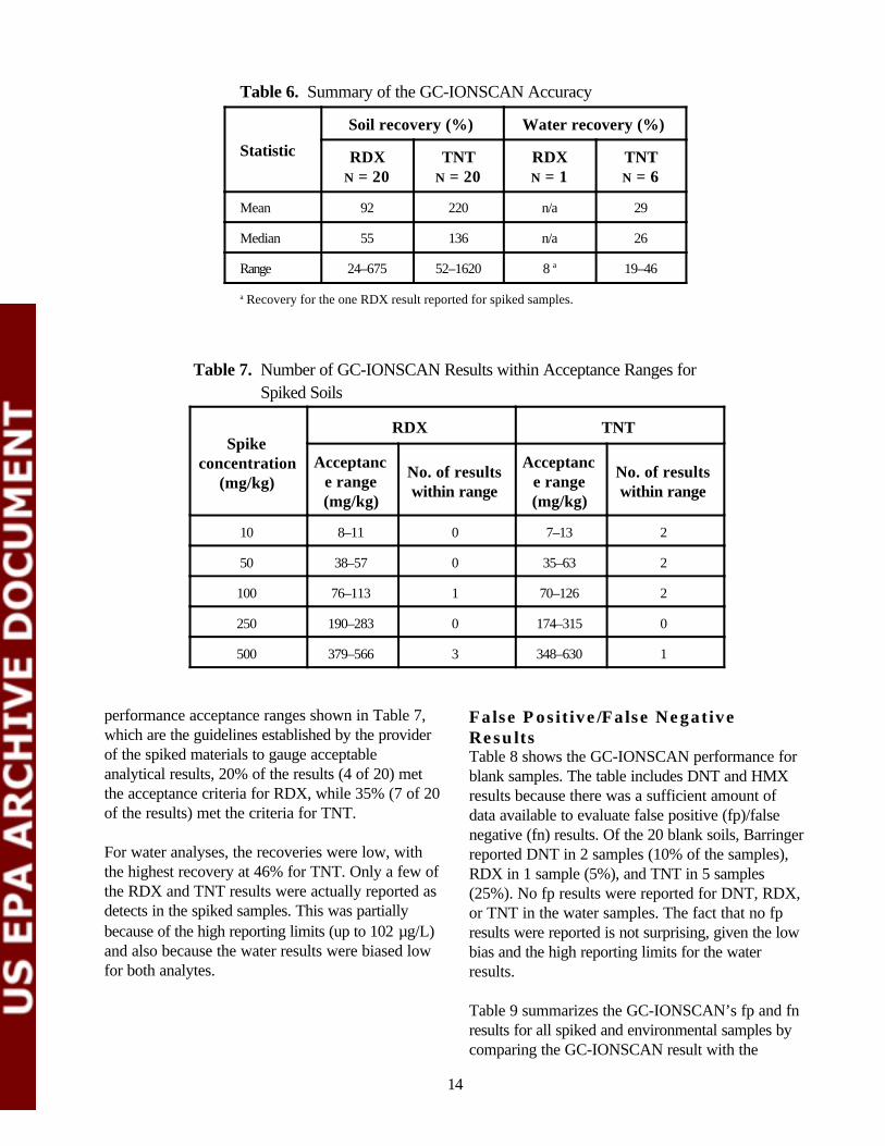
Table 6. Summary of the GC-IONSCAN Accuracy

Statistic

Soil recovery (%) Water recovery (%)

RDX N = 20

TNT N = 20

RDX N = 1

TNT N = 6

Mean 92 220 n/a 29

Median 55 136 n/a 26

Range 24–675 52–1620 8 a 19–46

a Recovery for the one RDX result reported for spiked samples.

Table 7. Number of GC-IONSCAN Results within Acceptance Ranges for Spiked Soils

Spike concentration

(mg/kg)

RDX TNT

Acceptanc e range (mg/kg)

No. of results within range

Acceptanc e range (mg/kg)

No. of results within range

10 8–11 0 7–13 2

50 38–57 0 35–63 2

100 76–113 1 70–126 2

250 190–283 0 174–315 0

500 379–566 3 348–630 1

performance acceptance ranges shown in Table 7, which are the guidelines established by the provider of the spiked materials to gauge acceptable analytical results, 20% of the results (4 of 20) met the acceptance criteria for RDX, while 35% (7 of 20 of the results) met the criteria for TNT.

For water analyses, the recoveries were low, with the highest recovery at 46% for TNT. Only a few of the RDX and TNT results were actually reported as detects in the spiked samples. This was partially because of the high reporting limits (up to 102 mg/L) and also because the water results were biased low for both analytes.

False Positive/False Negative Results Table 8 shows the GC-IONSCAN performance for blank samples. The table includes DNT and HMX results because there was a sufficient amount of data available to evaluate false positive (fp)/false negative (fn) results. Of the 20 blank soils, Barringer reported DNT in 2 samples (10% of the samples), RDX in 1 sample (5%), and TNT in 5 samples (25%). No fp results were reported for DNT, RDX, or TNT in the water samples. The fact that no fp results were reported is not surprising, given the low bias and the high reporting limits for the water results.

Table 9 summarizes the GC-IONSCAN’s fp and fn results for all spiked and environmental samples by comparing the GC-IONSCAN result with the

14

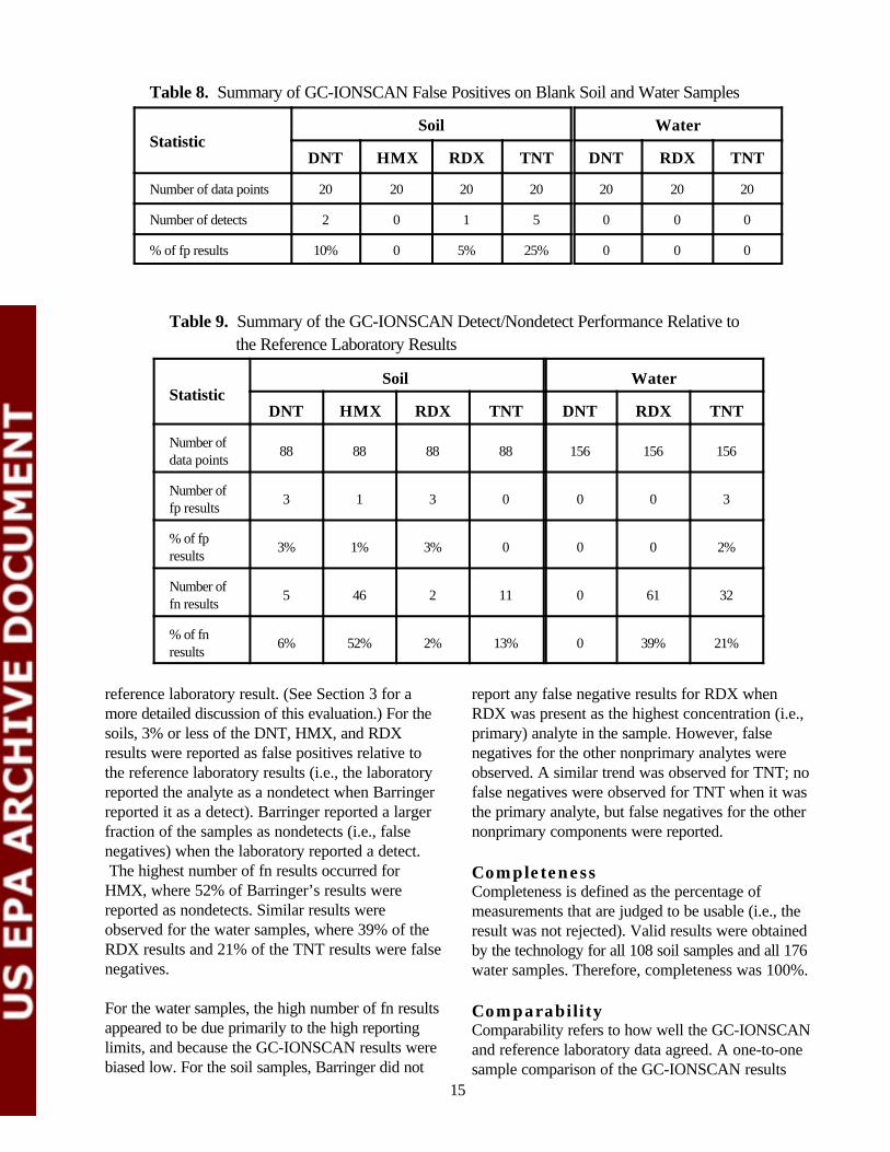
Table 8. Summary of GC-IONSCAN False Positives on Blank Soil and Water Samples


DNT HMX RDX TNT DNT RDX TNT

Number of data points 20 20 20 20 20 20 20

Number of detects 2 0 1 5 0 0 0

% of fp results 10% 0 5% 25% 0 0 0

Table 9. Summary of the GC-IONSCAN Detect/Nondetect Performance Relative to the Reference Laboratory Results


DNT HMX RDX TNT DNT RDX TNT

Number of data points 88 88 88 88 156 156 156

Number of fp results 3 1 3 0 0 0 3

% of fp results 3% 1% 3% 0 0 0 2%

Number of fn results 5 46 2 11 0 61 32

% of fn results 6% 52% 2% 13% 0 39% 21%

reference laboratory result. (See Section 3 for a more detailed discussion of this evaluation.) For the soils, 3% or less of the DNT, HMX, and RDX results were reported as false positives relative to the reference laboratory results (i.e., the laboratory reported the analyte as a nondetect when Barringer reported it as a detect). Barringer reported a larger fraction of the samples as nondetects (i.e., false negatives) when the laboratory reported a detect. The highest number of fn results occurred for HMX, where 52% of Barringer’s results were reported as nondetects. Similar results were observed for the water samples, where 39% of the RDX results and 21% of the TNT results were false negatives.

For the water samples, the high number of fn results appeared to be due primarily to the high reporting limits, and because the GC-IONSCAN results were biased low. For the soil samples, Barringer did not

report any false negative results for RDX when RDX was present as the highest concentration (i.e., primary) analyte in the sample. However, false negatives for the other nonprimary analytes were observed. A similar trend was observed for TNT; no false negatives were observed for TNT when it was the primary analyte, but false negatives for the other nonprimary components were reported.

Completeness Completeness is defined as the percentage of measurements that are judged to be usable (i.e., the result was not rejected). Valid results were obtained by the technology for all 108 soil samples and all 176 water samples. Therefore, completeness was 100%.

Comparability Comparability refers to how well the GC-IONSCAN and reference laboratory data agreed. A one-to-one sample comparison of the GC-IONSCAN results

15

and the reference laboratory results was performed for all environmental and spiked samples that were reported above the reporting limits. In Tables 10 and 11, the comparability of the results are presented in terms of correlation coefficients (r) and slopes (m).

The r value for the comparison of the entire soil data set of TNT results was 0.88 (m = 4.82). Note that including or excluding the unusual reference laboratory value does not cause this value to vary much. As shown in Table10, if comparability is assessed for specific concentration ranges, such as isolating those values less than 500 mg/kg, the r

value for TNT does not change dramatically, ranging from 0.71 to 0.85 depending on the concentrations selected.

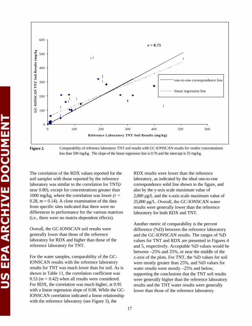
Figure 2 presents a plot of the GC-IONSCAN TNT results versus those for the reference laboratory for concentrations less than 500 mg/kg. The solid line on the graph is a representation of a one-to-one correspondence between the two measurements, while the dashed line is the linear regression line. As this figure indicates, the GC-IONSCAN soil measurements were generally higher than the reference laboratory results.

Table 10. GC-IONSCAN Correlation with Reference Data for Various Vendor Soil Concentration Ranges

Concentration RDX TNT

range r m r m

All values a 0.79 0.54 0.88 4.82

< 500 mg/kg b 0.79 0.52 0.71 0.76

< 1,000 mg/kg 0.89 0.27 0.77 0.96

> 1,000 mg/kg 0.28 0.14 0.85 5.32

> 10,000 mg/kg n/a c n/a 0.85 5.55

a Excluding those values reported as “< reporting limits” and including the one reference laboratory unusual value. (SeeSection 4 for more information on the unusual value.)b Based on Barringer’s reported values.c No RDX values above 10,000 mg/kg. were reported.

Table 11. GC-IONSCAN Correlation with Reference Data for Various Vendor WaterConcentration Ranges

Concentration RDX TNT

range r m r m

All values a 0.95 0.08 0.53 0.42

< 500 mg/L b 0.82 0.07 0.67 0.17

> 500 mg/L 0.87 0.06 0.32 0.25

> 1,000 mg/L –0.90 -0.08 –0.19 -0.11

a Excluding those values reported as “< reporting limits.” b Based on Barringer’s reported values.

16

r = 0.71

0

100

200

300

400

500

600

0 100 200 300 400 500 600

Reference Laboratory TNT Soil Results (mg/kg)

GC

-IO

NSC

AN

TN

T S

oil R

esul

ts (

mg/

kg)

one-to-one correspondence line

linear regression line

Figure 2. Comparability of reference laboratory TNT soil results with GC-IONSCAN results for vendor concentrations less than 500 mg/kg. The slope of the linear regression line is 0.76 and the intercept is 55 mg/kg.

The correlation of the RDX values reported for the soil samples with those reported by the reference laboratory was similar to the correlation for TNT(r near 0.80), except for concentrations greater than 1000 mg/kg, where the correlation was lower (r = 0.28, m = 0.14). A close examination of the data from specific sites indicated that there were no differences in performance for the various matrices (i.e., there were no matrix-dependent effects).

Overall, the GC-IONSCAN soil results were generally lower than those of the reference laboratory for RDX and higher than those of the reference laboratory for TNT.

For the water samples, comparability of the GC-IONSCAN results with the reference laboratory results for TNT was much lower than for soil. As is shown in Table 11, the correlation coefficient was 0.53 (m = 0.42) when all results were considered. For RDX, the correlation was much higher, at 0.95 with a linear regression slope of 0.08. While the GC-IONSCAN correlation indicated a linear relationship with the reference laboratory (see Figure 3), the

RDX results were lower than the reference laboratory, as indicated by the ideal one-to-one correspondence solid line shown in the figure, and also by the y-axis scale maximum value of 2,000 mg/L and the x-axis scale maximum value of 25,000 mg/L. Overall, the GC-IONSCAN water results were generally lower than the reference laboratory for both RDX and TNT.

Another metric of comparability is the percent difference (%D) between the reference laboratory and the GC-IONSCAN results. The ranges of %D values for TNT and RDX are presented in Figures 4 and 5, respectively. Acceptable %D values would be between –25% and 25%, or near the middle of the x-axis of the plots. For TNT, the %D values for soil were mostly greater than 25%, and %D values for water results were mostly –25% and below, supporting the conclusions that the TNT soil results were generally higher than the reference laboratory results and the TNT water results were generally lower than those of the reference laboratory.

17

r = 0.95

0

200

400

600

800

1,000

1,200

1,400

1,600

1,800

2,000

0 5,000 10,000 15,000 20,000 25,000

Reference Laboratory RDX Water Results (mm g/L)

GC

-IO

NSC

AN

RD

X W

ater

Res

ults

( mm

g/L

)

one-to-one correspondence line

linear regression line

Figure 3. Comparability of reference laboratory RDX water results with GC-IONSCAN results for all results reported above reporting limits. The slope of the linear regression line is 0.08, and the intercept is 51 mg/L.

As shown in Figure 5, most of the %D values for RDX were negative, supporting the conclusion that the GC-IONSCAN RDX results, particularly for water, were lower than the reference laboratory.

Sample Throughput Sample throughput is representative of the estimated amount of time required to prepare and analyze the sample. Operating under the outdoor conditions, the two-person Barringer team accomplished a sample throughput rate of approximately three samples per hour for soil and eight samples per hour for water.

Ease of Use Two operators were used for the demonstration because of the number of demonstration samples and working conditions, but the technology can be operated by a single person. Users unfamiliar with ion mobility spectrometry would need approximately two days of training to operate the GC-IONSCAN. Barringer Instruments provides

training with instrument installation. No particular level of educational training is required for the operator, but skills in chromatographic techniques would be advantageous.

Cost Assessment The purpose of this economic analysis is to estimate the range of costs for analysis of explosivescontaminated soil and water samples using the GC-IONSCAN and a conventional analytical reference laboratory method. The analysis was based on the results and experience gained from this demonstration, costs provided by Barringer, and representative costs provided by the reference analytical laboratories that offered to analyze these samples. To account for the variability in cost data and assumptions, the economic analysis is presented as a list of cost elements and a range of costs for sample analysis by the GC-IONSCAN instrument and by the reference laboratory.

18

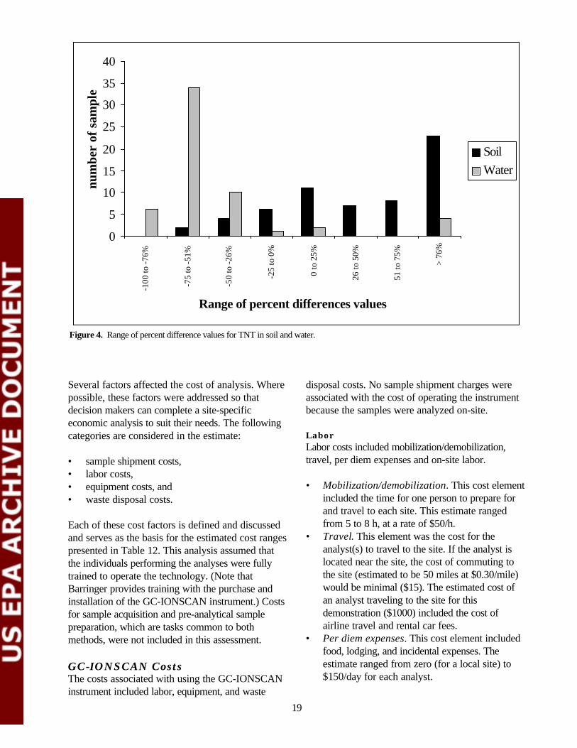
0

5

10

15

20

25

30

35

40

-100

to -7

6%

-75

to -5

1%

-50

to -2

6%

-25

to 0

%

0 to

25%

26 to

50%

51 to

75%

> 76

%

Range of percent differences values

num

ber

of s

ampl

es

Soil Water

Figure 4. Range of percent difference values for TNT in soil and water.

Several factors affected the cost of analysis. Where possible, these factors were addressed so that decision makers can complete a site-specific economic analysis to suit their needs. The following categories are considered in the estimate:

• sample shipment costs, • labor costs, • equipment costs, and • waste disposal costs.

Each of these cost factors is defined and discussed and serves as the basis for the estimated cost ranges presented in Table 12. This analysis assumed that the individuals performing the analyses were fully trained to operate the technology. (Note that Barringer provides training with the purchase and installation of the GC-IONSCAN instrument.) Costs for sample acquisition and pre-analytical sample preparation, which are tasks common to both methods, were not included in this assessment.

GC-IONSCAN Costs The costs associated with using the GC-IONSCAN instrument included labor, equipment, and waste

disposal costs. No sample shipment charges were associated with the cost of operating the instrument because the samples were analyzed on-site.

Labor Labor costs included mobilization/demobilization, travel, per diem expenses and on-site labor.

• Mobilization/demobilization. This cost element included the time for one person to prepare for and travel to each site. This estimate ranged from 5 to 8 h, at a rate of $50/h.

• Travel. This element was the cost for the analyst(s) to travel to the site. If the analyst is located near the site, the cost of commuting to the site (estimated to be 50 miles at $0.30/mile) would be minimal ($15). The estimated cost of an analyst traveling to the site for this demonstration ($1000) included the cost of airline travel and rental car fees.

• Per diem expenses. This cost element included food, lodging, and incidental expenses. The estimate ranged from zero (for a local site) to $150/day for each analyst.

19

0

5

10

15

20

25

30

-100

to -7

6%

-75

to -5

1%

-50

to -2

6%

-25

to 0

%

0 to

25%

26 to

50%

51 to

75%

> 76

%

Range of percent difference values

num

ber

of s

ampl

es

Soil Water

Figure 5. Range of percent difference values for RDX in soil and water.

• Rate. The cost of the on-site labor was estimated at a rate of $30–75/h, depending on the required expertise level of the analyst. This cost element included the labor involved with the entire analytical process, comprising sample preparation, sample management, analysis, and reporting.

Equipment Equipment costs included mobilization/ demobilization, rental fees or purchase of equipment, and the reagents and other consumable supplies necessary to complete the analysis.

• Mobilization/demobilization. This included the cost of shipping the equipment to the test site. If the site is local, the cost would be zero. For this demonstration, the cost of shipping equipment and supplies was estimated at $150.

• Instrument purchase. At the time of the demonstration, the cost of purchasing the GC-IONSCAN was $60,000. The purchase included a laptop computer, four kits (a standard spare kit, a standard maintenance kit, a standard consumables kit, and a sampling kit), a swab sampler, IM software, an operators’ manual, and training at Barringer for up to six people. The kit

is supplied in an aluminum carrying case. The instrument can be operated in two modes; explosives detection and drug detection. As with any instrument, the cost on a per-sample basis would decrease as the number of analyses performed increases.

• Reagents/supplies. These items are consumable and are purchased on a per sample basis. At the time of the demonstration, the cost of the reagents and supplies needed to prepare and analyze explosives samples using the GC-IONSCAN was $1 per sample. This cost included the sample preparation supplies, assay supplies, and consumable reagents.

Waste Disposal Waste disposal costs are based on the 1999 regulations for disposal of explosives-contaminated waste. The analyses performed using the GC-IONSCAN instrument generated approximately 70 lb of vials (two 5-gal buckets) containing soils and liquid solvents. ORNL’s cost to dispose of the explosives-contaminated waste at a commercial facility was estimated at $90 per 5-gal bucket. There are most likely additional costs for labor associated with the waste disposal, but those costs are not estimated here.

20

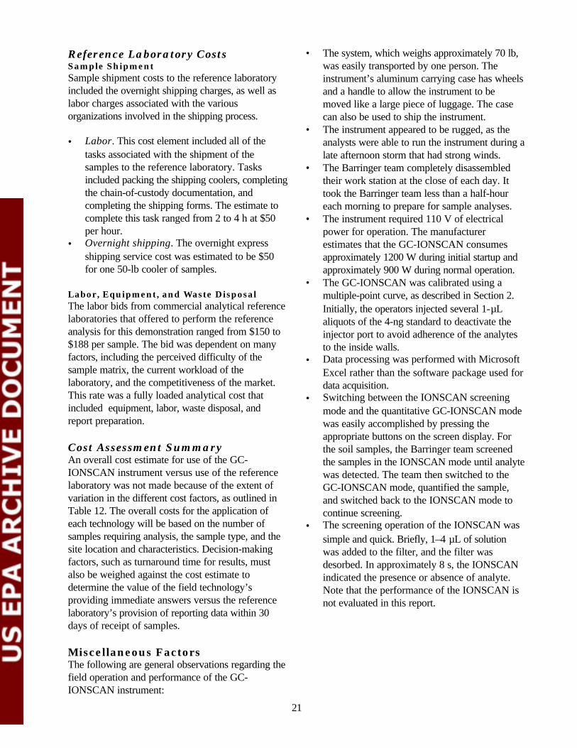
Reference Laboratory Costs Sample Shipment Sample shipment costs to the reference laboratory included the overnight shipping charges, as well as labor charges associated with the various organizations involved in the shipping process.

• Labor. This cost element included all of the tasks associated with the shipment of the samples to the reference laboratory. Tasks included packing the shipping coolers, completing the chain-of-custody documentation, and completing the shipping forms. The estimate to complete this task ranged from 2 to 4 h at $50 per hour.

• Overnight shipping. The overnight express shipping service cost was estimated to be $50 for one 50-lb cooler of samples.

Labor, Equipment, and Waste Disposal The labor bids from commercial analytical reference laboratories that offered to perform the reference analysis for this demonstration ranged from $150 to $188 per sample. The bid was dependent on many factors, including the perceived difficulty of the sample matrix, the current workload of the laboratory, and the competitiveness of the market. This rate was a fully loaded analytical cost that included equipment, labor, waste disposal, and report preparation.

Cost Assessment Summary An overall cost estimate for use of the GC-IONSCAN instrument versus use of the reference laboratory was not made because of the extent of variation in the different cost factors, as outlined in Table 12. The overall costs for the application of each technology will be based on the number of samples requiring analysis, the sample type, and the site location and characteristics. Decision-making factors, such as turnaround time for results, must also be weighed against the cost estimate to determine the value of the field technology’s providing immediate answers versus the reference laboratory’s provision of reporting data within 30 days of receipt of samples.

Miscellaneous Factors The following are general observations regarding the field operation and performance of the GC-IONSCAN instrument:

• The system, which weighs approximately 70 lb, was easily transported by one person. The instrument’s aluminum carrying case has wheels and a handle to allow the instrument to be moved like a large piece of luggage. The case can also be used to ship the instrument.

• The instrument appeared to be rugged, as the analysts were able to run the instrument during a late afternoon storm that had strong winds.

• The Barringer team completely disassembled their work station at the close of each day. It took the Barringer team less than a half-hour each morning to prepare for sample analyses.

• The instrument required 110 V of electrical power for operation. The manufacturer estimates that the GC-IONSCAN consumes approximately 1200 W during initial startup and approximately 900 W during normal operation.

• The GC-IONSCAN was calibrated using a multiple-point curve, as described in Section 2. Initially, the operators injected several 1-mL aliquots of the 4-ng standard to deactivate the injector port to avoid adherence of the analytes to the inside walls.

• Data processing was performed with Microsoft Excel rather than the software package used for data acquisition.

• Switching between the IONSCAN screening mode and the quantitative GC-IONSCAN mode was easily accomplished by pressing the appropriate buttons on the screen display. For the soil samples, the Barringer team screened the samples in the IONSCAN mode until analyte was detected. The team then switched to the GC-IONSCAN mode, quantified the sample, and switched back to the IONSCAN mode to continue screening.

• The screening operation of the IONSCAN was simple and quick. Briefly, 1–4 mL of solution was added to the filter, and the filter was desorbed. In approximately 8 s, the IONSCAN indicated the presence or absence of analyte. Note that the performance of the IONSCAN is not evaluated in this report.

21

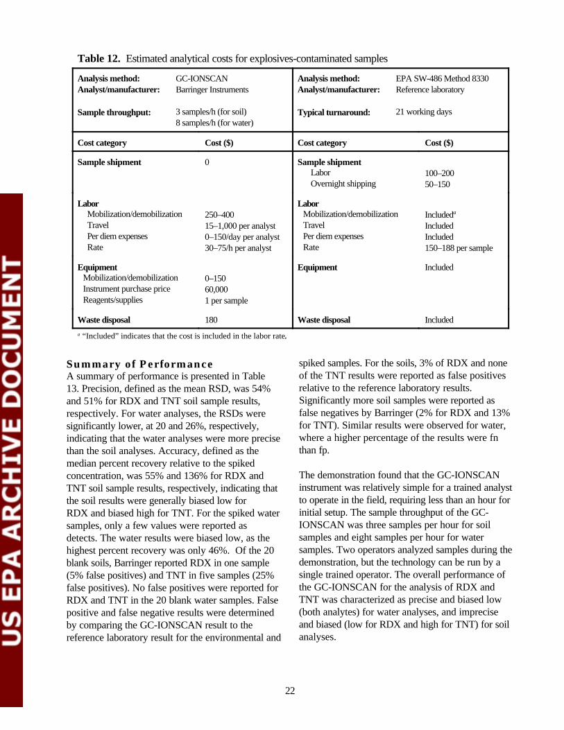
Table 12. Estimated analytical costs for explosives-contaminated samples

Analysis method: GC-IONSCAN Analyst/manufacturer: Barringer Instruments

Sample throughput: 3 samples/h (for soil) 8 samples/h (for water)

Analysis method: Analyst/manufacturer:

Typical turnaround:

EPA SW-486 Method 8330 Reference laboratory

21 working days

Cost category Cost ($) Cost category Cost ($)

Sample shipment 0

Labor Mobilization/demobilization Travel Per diem expenses Rate

250–400 15–1,000 per analyst 0–150/day per analyst 30–75/h per analyst

Equipment Mobilization/demobilization Instrument purchase price Reagents/supplies

0–150 60,000 1 per sample

Waste disposal 180

Sample shipment Labor Overnight shipping

Labor Mobilization/demobilization Travel Per diem expenses Rate

Equipment

Waste disposal

100–200 50–150

Includeda

Included Included 150–188 per sample

Included

Included a “Included” indicates that the cost is included in the labor rate.

Summary of Performance A summary of performance is presented in Table 13. Precision, defined as the mean RSD, was 54% and 51% for RDX and TNT soil sample results, respectively. For water analyses, the RSDs were significantly lower, at 20 and 26%, respectively, indicating that the water analyses were more precise than the soil analyses. Accuracy, defined as the median percent recovery relative to the spiked concentration, was 55% and 136% for RDX and TNT soil sample results, respectively, indicating that the soil results were generally biased low for RDX and biased high for TNT. For the spiked water samples, only a few values were reported as detects. The water results were biased low, as the highest percent recovery was only 46%. Of the 20 blank soils, Barringer reported RDX in one sample (5% false positives) and TNT in five samples (25% false positives). No false positives were reported for RDX and TNT in the 20 blank water samples. False positive and false negative results were determined by comparing the GC-IONSCAN result to the reference laboratory result for the environmental and

spiked samples. For the soils, 3% of RDX and none of the TNT results were reported as false positives relative to the reference laboratory results. Significantly more soil samples were reported as false negatives by Barringer (2% for RDX and 13% for TNT). Similar results were observed for water, where a higher percentage of the results were fn than fp.

The demonstration found that the GC-IONSCAN instrument was relatively simple for a trained analyst to operate in the field, requiring less than an hour for initial setup. The sample throughput of the GC-IONSCAN was three samples per hour for soil samples and eight samples per hour for water samples. Two operators analyzed samples during the demonstration, but the technology can be run by a single trained operator. The overall performance of the GC-IONSCAN for the analysis of RDX and TNT was characterized as precise and biased low (both analytes) for water analyses, and imprecise and biased (low for RDX and high for TNT) for soil analyses.

22

Table 13. Performance Summary for the GC-IONSCAN

Feature/Parameter Performance summary

Precision Mean RSD Soil: 54% RDX, 51% TNT Water: 20% RDX , 26% TNT

Accuracy Median recovery Soil: 55% RDX, 136% TNT Water: n/a (see Table 6); 26% TNT

False positive results on blank samples

Soil: 10% DNT, 0% HMX, 5% RDX, 25% TNT Water: 0% DNT, 0% RDX, 0% TNT

False positive results relative to reference laboratory results

Soil: 3% DNT, 1% HMX, 3% RDX, 0% TNT Water: 0% DNT, 0% RDX, 2% TNT

False negative results relative to reference laboratory results

Soil: 6% DNT, 52% HMX, 2% RDX (0% if RDX was the highest concentration analyte), 13% TNT (0% if TNT was the highest concentration analyte)

Water: 0% DNT, 39% RDX, 21% TNT

Comparison with reference laboratory results

r (all results) m (all results) Soil: 0.79 RDX, 0.88 TNT 0.54 RDX, 4.82 TNT Water: 0.95 RDX, 0.53 TNT 0.08 RDX, 0.42 TNT

Median %D range of %D values Soil: –46% RDX, 51% TNT –83 to 562% RDX, –70 to 1500% TNT Water: –90% RDX, –59% TNT –97 to –82% RDX, –88 to 1310%

TNT

Completeness 100% of 108 soil samples 100% of 176 water samples

Weight 70 lb

Sample throughput (2 operators) Soil: 3 samples/h Water: 8 samples/h

Power requirements 110 V, 60 Hz 1200 W startup 900 W normal operations

Training requirements Two days instrument-specific training

Cost Instrument: $60,000 Supplies per sample: $1

Hazardous waste generation Two 5-gal buckets filled with vials containing acetone extracts of samples, empty vials, and pipette tips (Total number of samples analyzed: 108 soils and 176 waters)

Overall evaluation Soil: biased low for RDX and biased high for TNT; imprecise Water: biased low for RDX and TNT; precise Insufficient data to evaluate performance on DNT and HMX

23

Section 6 — Technology Update

In this section, the vendor (with minimal editorial changes by ORNL) provides comments regarding the use and the performance of the GC-IONSCAN during verification testing and information regarding new developments with the technology since the verification activities.

Barringer’s past experience has been in the area of rapid prescreening of surfaces for traces of narcotics or explosives on a semiquantitative level. This field trial was Barringer’s first formal attempt at the rapid quantitative screening of water and soil samples. Barringer believes that future improvements in the simple sample preparation methodology used to extract explosives from water and soil will significantly improve agreement with laboratory-based data.

Rapid Prescreening of Samples Part of Barringer’s method includes using the IONSCAN mode to rapidly prescreen all the soil samples before GC-IONSCAN analysis. In the IONSCAN mode the operator can screen samples at a much higher throughput rate than in the GC-IONSCAN mode, since the instrument analysis time in IONSCAN mode is less than 10 s per sample. During verification testing, if no DNT, HMX, RDX, or TNT was detected, then GC-IONSCAN analysis was not performed. IONSCAN mode performance was not verified by ETV, but Barringer observed that rapid prescreening during the ETV trial correctly identified the presence of explosives in 100% of the samples that contained explosives and was able to screen out 35% of the blank samples from full GC-IONSCAN analysis.1 With an

appropriate setting of threshold detection levels, Barringer believes a larger number of blank samples could have been screened out.

Improvements to GC-IONSCAN The GC-IONSCAN unit evaluated in this trial was one of the first prototypes built. Since this trial, significant improvements have been made to the GC-IONSCAN instrument and firmware. The position of thermocouples in the oven has been changed to ensure that the oven is uniformly heated and to improve circulation in the unit. An additional fan has added to allow faster cooling of the unit after temperature has been ramped; this feature will increase sample throughput. The carrier gas pressure reading is now displayed to an extra significant digit (i.e., 12 to 12.0 PSI) to permit more reproducible settings of pressure. Upgrading of the firmware of the unit to improve the peak finding routine for the GC data should help minimize false positives for DNT. The temperature controller for the transfer line between the end of the GC column and the IONSCAN has been upgraded to permit temperatures above 190ºC. This upgrade will help minimize sample losses for HMX and decrease the false negative rate for HMX. Note that samples can be injected either split or splitless.

1 Data analysis performed by Barringer and not ETV-verified. 24

Section 7 — References

Berger, W., H. McCarty, and R-K. Smith. 1996. Environmental Laboratory Data Evaluation. Genium Publishing Corp., Schenectady, N.Y.

Draper, N. R., and H. Smith. 1981. Applied Regression Analysis. 2nd ed. John Wiley & Sons, New York.

EPA (U.S. Environmental Protection Agency). 1994. “Method 8330: Nitroaromatics and Nitramines by High Performance Liquid Chromatography (HPLC).” In Test Methods for Evaluating Solid Waste: Physical/ Chemical Methods, Update II. SW-846. U.S. Environmental Protection Agency, Washington, D.C., September.

EPA (U.S. Environmental Protection Agency). 1998. EPA Guidance for Quality Assurance Project Plans. EPA QA/G-5, EPA 600/R-98/018. U.S. Environmental Protection Agency, Washington, D.C., February.

Jenkins, T. F., M. E. Walsh, and P. G. Thorne. 1998. “Site Characterization for Explosives Contamination at a Military Firing Range Impact Area.” Special Report 98-9. U.S. Army Cold Regions Research and Engineering Laboratory, Hanover, N.H. Available at http://www.crrel.usace.army.mil/

Maskarinec, M. P., C. K. Bayne, L. H. Johnson, S. K. Holladay, R. A. Jenkins, and B. A. Tomkins. 1991. Stability of Explosives in Environmental Water and Soil Samples. ORNL/TM-11770. Oak Ridge National Laboratory, Oak Ridge, Tenn., January.

ORNL (Oak Ridge National Laboratory). 1999. “Technology Demonstration Plan: Evaluation of Explosives Field Analytical Techniques.” Oak Ridge National Laboratory, Oak Ridge, Tenn., August.

Specialized Assays, Inc. 1999. “Comprehensive Quality Assurance Plan.” SAL-QC-Rec 5.0. January 6.

25

http://www.crrel.usace.army.mil/

Appendix A

GC-IONSCAN Sample Soil Results Compared withReference Laboratory Results

29

Table A-1. GC-IONSCAN Sample Soil Results Compared with Reference Laboratory Results

Sample site or type

Sample no.

Sample replicate

DNT a

(mg/kg)

Barringer Ref Lab

HMX a

(mg/kg)

Barringer Ref Lab

RDX a

(mg/kg)

Barringer Ref Lab

TNT a

(mg/kg)

Barringer Ref Lab

Barringer analysis order b

Blank Blank Blank Blank

1 1 1 1

1 2 3 4

<10.0 <10.0 <10.0 <10.0

<0.5 <0.5 <0.5 <0.5

<0.6 <0.6 <0.6 <0.6

<0.5 <0.5 <0.5 <0.5

<0.6 <0.6 <0.3 <0.6

<0.5 <0.5 <0.5 <0.5

<0.6 1.9

<0.6 <0.6

<0.5 <0.5 <0.5 <0.5

1090 1077 1066 1101


2 2 2 2

1 2 3 4

297.1 <10.0 <10.0 <12.5

<0.5 <51.0 <0.5 <0.5

<0.3 <0.6 <0.6 <0.3

<0.5 <51.0 <0.5 <0.5

<0.3 <0.3 <0.3 <0.3

<0.5 <51.0 <0.5 <0.5

<0.3 0.9 1

<0.3

<0.5 70900 <0.5 <0.5

1013 1032 1031 1001


3 3 3 3

1 2 3 4

<10.0 <10.0 <10.0 <10.0

<0.5 <0.5 <0.5 <0.5

<0.6 <0.6 <0.6 <0.6

<0.5 <0.5 <0.5 <0.5

<0.3 <0.3 <0.3 18.8

<0.5 <0.5 <0.5 <0.5

52.2 <0.6 <0.6 <0.6

<0.5 <0.5 <0.5 <0.5

1051 1027 1055 1036


4 4 4 4

1 2 3 4

<10.0 <10.0 <10.0 1163.9

<0.5 <0.5 <0.5 <0.5

<0.6 <0.6 <0.6 <0.3

<0.5 <0.5 <0.5 <0.5

<0.6 <0.3 <0.3 <0.3

<0.5 <0.5 <0.5 <0.5

<0.6 <0.6 <0.6 <0.3

0.9 <0.5 <0.5 <0.5

1086 1026 1070 1007


5 5 5 5

1 2 3 4

<10.0 <10.0 <10.0 <10.0

<0.5 <0.5 <0.5 <0.5

<0.6 <0.6 <0.6 <0.6

<0.5 <0.5 <0.5 <0.5

<0.3 <0.6 <0.3 <0.3

<0.5 <0.5 <0.5 <0.5

<0.6 <0.6 1.5

<0.6

<0.5 <0.5 <0.5 <0.5

1021 1095 1064 1048

Fort Ord Fort Ord Fort Ord Fort Ord

1 1 1 1

1 2 3 4

<10.0 <10.0 <10.0 <10.0

<0.5 <0.5 <0.5 <0.5

DI b

22 DI DI

370 252 259 264

<0.3 <0.3 <0.6 <0.6

0.6 <0.5 <0.5 0.5

<0.6 0.9

<1.3 <1.3

<0.5 0.8 0.8

<0.5

1065 1025 1083 1078


2 2 2 2

1 2 3 4

<10.0 <10.0 <10.0 <10.0

<0.5 <0.5 <0.5 <0.5

DI 50.1 <0.6 DI

278 248 322 185

<0.6 <0.3 <0.3 <0.3

<0.5 <0.5 <0.5 <0.5

<1.3 1.6

<0.6 1

0.8 2.1 0.8 0.8

1079 1030 1038 1060


3 3 3 3

1 2 3 4

<10.0 <10.0 <10.0 <10.0

<0.5 <0.5 <0.5 <0.5

DI 28.3 <0.6 DI

300 185 392 214

<0.3 <0.3 <0.3 1.9

<0.5 <0.5 <0.5 <0.5

<0.6 <0.6 <0.6 <0.6

<0.5 <0.5 <0.5 <0.5

1057 1017 1046 1087

30

Sample site or type

Sample no.

Sample replicate

DNT a

(mg/kg)

Barringer Ref Lab

HMX a

(mg/kg)

Barringer Ref Lab

RDX a

(mg/kg)

Barringer Ref Lab

TNT a

(mg/kg)

Barringer Ref Lab


Iowa Iowa Iowa Iowa

1 1 1 1

1 2 3 4

<12.5 <10.0 <10.0 <10.0

<51.0 <0.5

<532.0 <50.5

<0.3 <0.6 <0.6 <0.6

<51.0 <0.5

<532.0 <50.5

<0.3 <0.6 <0.6 <0.3

<51.0 <0.5

<532.0 <50.5

30195.6 50310

53214.9 75814.5

20400 0.8

33400 28300

1008 1080 1076 1047

Louisiana Louisiana Louisiana Louisiana

1 1 1 1

1 2 3 4

<10.0 <10.0 <10.0 <10.0

<0.5 <0.5 <0.5 <25.0

69.6 <0.6 DI DI

400 460 202 470

2342.7 821.6 2164.8 2414.2

3460 3520 2140 1900

178.9 <0.6 <0.6 <0.6

109 120 111 125

1029 1012 1098 1105


2 2 2 2

1 2 3 4

<10.0 <10.0 <10.0 <10.0

<0.5 <0.5 <0.5 <0.5

<0.6 <0.6 <0.6 <0.6

100 204 153 25.6

1378.3 1115.5 1177.1 455.4

1180 1450 1170 320

<0.6 206 <0.6 59.5

50 51 51

10.6

1094 1042 1022 1049


3 3 3 3

1 2 3 4

<10.0 <10.0 <10.0 <10.0

<0.5 <50.0 <50.0 <0.5

<0.6 <0.6 DI

<0.6

360 470 390 500

1833.5 2169.4 3527.9 1195.4

4300 3550 4650 5850

303.4 471.9 166.8 271.2

205 170 300 400

1073 1045 1091 1043


4 4 4 4

1 2 3 4

<10.0 <10.0 <10.0 <10.0

80 11.4 11.9 9.5

<0.6 <0.6 <0.6 <0.6

<5.0 <0.5 <0.5 0.5

2.1 5

5.5 2.9

12 10.7 10.8 7.7

104 162.8 102.5 158.7

89 78

81.5 67.5

1099 1034 1096 1084

Milan Milan Milan Milan

1 1 1 1

1 2 3 4

<10.0 1069.3 <10.0 <10.0

<0.5 <0.5 <0.5 <0.5

DI <0.3 <0.6 <0.6

22.2 23.2 16.5 42

41.9 52.3 36.8 85.6

149 118 72.2 308

<0.6 <0.3 <0.6 <0.6

2.7 1.1 1.4 1.7

1062 1010 1053 1108


2 2 2 2

1 2 3 4

<10.0 <12.5 <12.5 <10.0

<0.5 <0.5 <0.5 <0.5

<0.6 <0.3 <0.3 <0.6

8.3 3.6 3.5 4.3

7.4 9.2 50 9.5

34.8 16.4 28

22.9

<0.6 <0.3 <0.3 <1.3

<0.5 <0.5 <0.5 <0.5

1059 1006 1002 1075


3 3 3 3

1 2 3 4

<10.0 <10.0 <10.0 <10.0

<0.5 <50.0 <200.0 <0.5

<0.6 88.5 <0.6 DI

330 420 400 343

3082.3 2775.5 2814.5 2735.6

2350 1950 4080 3880

319.7 624.8 204.3 205.4

190 270 320 273

1005 1023 1102 1097

Milan 4 1 <10.0 <50.0 42.7 240 893.9 2740 282.6 220 1024

31

Sample site or type

Sample no.

Sample replicate

DNT a

(mg/kg)

Barringer Ref Lab

HMX a

(mg/kg)

Barringer Ref Lab

RDX a

(mg/kg)

Barringer Ref Lab

TNT a

(mg/kg)

Barringer Ref Lab


Milan Milan Milan

4 4 4

2 3 4

<10.0 <10.0

372961

<0.5 <0.5 <0.5

<0.6 DI

73.4

260 405 222

3012.3 2005.1 869.3

2640 2600 3070

<0.6 207.9 467.5

260 80 162

1016 1081 1039


5 5 5 5

1 2 3 4

<10.0 <10.0 <10.0 <10.0

3.6 2.7 3.4 3.8

<0.6 DI

<0.6 <0.6

<0.5 <0.5 <0.5 <0.5

0.7 <0.6 <0.6 <0.3

<0.5 <0.5 <0.5 <0.5

14.2 5.2 5.6 15.2

11.5 10.2 11.3 10.6

1074 1089 1104 1054

Spike/PE Spike/PE Spike/PE Spike/PE

1 1 1 1

1 2 3 4

<10.0 <10.0 <10.0 <10.0

<0.5 <0.5 <0.5 <0.5

<0.6 <0.6 <0.6 <0.6

<0.5 <0.5 <0.5 <0.5

<0.3 <0.3 <0.3 <0.3

<0.5 <0.5 <0.5 <0.5

180.4 107.9 93.8 143.4

81.8 104 90 124

1033 1072 1015 1063


2 2 2 2

1 2 3 4

<10.0 <10.0 <10.0 <10.0

<0.5 <0.5 <0.5 <0.5

<0.6 <0.6 <0.6 <0.6

1.5 1.1 1.2 1.4

54.8 96.5 149.3 23.8

111 90.5 98 127

<0.6 <0.6 <0.6 <0.6

<0.5 <0.5 <0.5 <0.5

1035 1019 1092 1068


3 3 3 3

1 2 3 4

<10.0 <10.0 <10.0 <10.0

<0.5 <0.5 <0.5 <0.5

DI <0.6 <0.6 <0.6

0.5 0.8 1.1 0.8

14.4 32.6 13.5 27.4

49.5 45

63.5 51

16.4 17.2 12 11

8.4 7.6 10 8.5

1061 1100 1071 1107


4 4 4 4

1 2 3 4

566.2 <10.0 <12.5 <10.0

<0.5 <0.5 <0.5 <0.5

<0.3 <0.6 <0.3 <0.6

<0.5 <0.5 <0.5 <0.5

5.1 5.4 4.5 3.5

9.1 8.4 8.6 9.1

56.3 119.3 41.2 65.3

47.5 48.5 48.5 47

1003 1044 1011 1069


5 5 5 5

1 2 3 4

<10.0 <10.0 <10.0 <10.0

<0.5 <0.5 <0.5 <0.5

DI <0.6 <0.6 <0.6

5.9 6.3 8.8 6.9

119.3 560.4 382

528.3

460 455 705 445

597.6 335.8 129.1 343.8

230 205 435 205

1058 1018 1088 1020


6 6 6 6

1 2 3 4

<10.0 <10.0 <10.0 <10.0

<0.5 <25.0 <0.5 <0.5

<0.6 <0.6 <0.6 <0.6

<25.0 <25.0 <25.0

3.7

126.6 1687 138.7 154

260 255 335 250

1533 8104.3 793.6 465.4

535 505 675 510

1040 1014 1082 1093

Volunteer Volunteer Volunteer

1 1 1

1 2 3

<10.0 <12.5 <10.0

<50.0 <25.0

19

<0.6 <0.3 <0.6

<50.0 <25.0 <5.0

<0.3 <0.3 <0.3

<50.0 <25.0 <5.0

361997 115876 898117

108000 75500 117000

1037 1009 1050

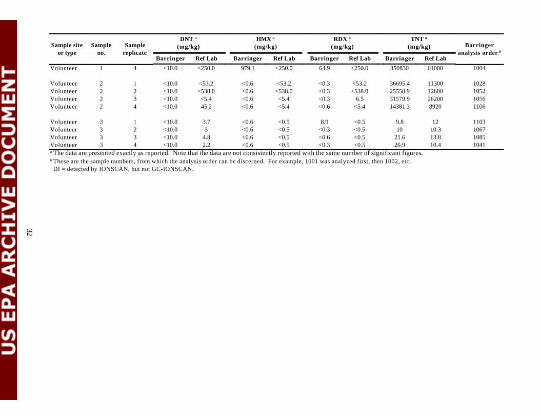
DNT a HMX a RDX a TNT a

Sample site Sample Sample (mg/kg) (mg/kg) (mg/kg) (mg/kg) Barringer or type no. replicate analysis order b

Barringer Ref Lab Barringer Ref Lab Barringer Ref Lab Barringer Ref Lab

Volunteer 1 4 <10.0 <250.0 979.1 <250.0 64.9 <250.0 350830 61000 1004

Volunteer 2 1 <10.0 <53.2 <0.6 <53.2 <0.3 <53.2 36695.4 11300 1028 Volunteer 2 2 <10.0 <538.0 <0.6 <538.0 <0.3 <538.0 25550.9 12600 1052 Volunteer 2 3 <10.0 <5.4 <0.6 <5.4 <0.3 6.5 31579.9 26200 1056 Volunteer 2 4 <10.0 45.2 <0.6 <5.4 <0.6 <5.4 14381.3 8920 1106

Volunteer 3 1 <10.0 3.7 <0.6 <0.5 8.9 <0.5 9.8 12 1103 Volunteer 3 2 <10.0 3 <0.6 <0.5 <0.3 <0.5 10 10.3 1067 Volunteer 3 3 <10.0 4.8 <0.6 <0.5 <0.6 <0.5 21.6 13.8 1085 Volunteer 3 4 <10.0 2.2 <0.6 <0.5 <0.3 <0.5 20.9 10.4 1041 a The data are presented exactly as reported. Note that the data are not consistently reported with the same number of significant figures. b These are the sample numbers, from which the analysis order can be discerned. For example, 1001 was analyzed first, then 1002, etc. DI = detected by IONSCAN, but not GC-IONSCAN.

32

Appendix B

GC-IONSCAN Sample Water Results Compared withReference Laboratory Results

35

Table B-1. GC-IONSCAN Sample Water Results Compared with Reference Laboratory Results

Sample site or type

Sample no. Sample replicate

DNT a

(mmg/L)

Barringer Ref Lab

RDX a

(mmg/L)

Barringer Ref Lab

TNT a

(mmg/L)

Barringer Ref Lab

Barringer analysis orderb


6 6 6 6

1 2 3 4

<1950.0 <1950.0 <1950.0 <1950.0

<0.5 <0.5 <0.5 <0.5

<51.3 <25.6 <102.5 <102.5

1.5 <0.5 <0.5 <0.5

<72.5 <36.3 <58.0 <58.0

1.9 1.2

<0.5 <0.5

2066 2007 2133 2132


7 7 7 7

1 2 3 4

<1950.0 <1950.0 <1950.0 <1950.0

<0.5 <0.5 <0.5 <0.5

<51.3 <51.3 <102.5 <51.3

<0.5 <0.5 <0.5 <0.5

<72.5 <72.5 <58.0 <72.5

<0.5 0.9

<0.5 <0.5

2039 2063 2147 2071


8 8 8 8

1 2 3 4

<1950.0 <1950.0 <1950.0 <1950.0

<0.5 <0.5 <0.5 <0.5

<102.5 <102.5 <51.3 <51.3

<0.5 <0.5 0.5

<0.5

<58.0 <58.0 <72.5 <72.5

<0.5 <0.5 <0.5 1.3

2131 2153 2061 2097


9 9 9 9

1 2 3 4

<1950.0 <1950.0 <1950.0 <1950.0

<0.5 0.6

<0.5 <0.5

<51.3 <25.6 <102.5 <102.5

<0.5 <0.5 <0.5 <0.5

<72.5 <36.3 <58.0 <58.0

<0.5 <0.5 <0.5 <0.5

2045 2012 2134 2142


10 10 10 10

1 2 3 4

<1950.0 <1950.0 <1950.0 <1950.0

<0.5 <0.5 <0.5 <0.5

<51.3 <102.5 <102.5 <102.5

<0.5 <0.5 <0.5 <0.5

<72.5 <58.0 <58.0 <58.0

<0.5 <0.5 <0.5 <0.5

2055 2168 2145 2121


5 5 5 5

1 2 3 4

<1950.0 <1950.0 <1950.0 <1950.0

<0.5 <0.5 <0.5 <0.5

<51.3 <102.5 <51.3 <51.3

200 159 180 158

<72.5 <58.0 <72.5 <72.5

170 136 151 138

2077 2146 2042 2052


6 6 6 6

1 2 3 4

<1950.0 <1950.0 <1950.0 <1950.0

<0.5 <0.5 <0.5 0.5

<102.5 <102.5 <51.3 <51.3

210 238 160 256

<58.0 67.6

<72.5 <72.5

162 176 113 178

2151 2172 2051 2032

Louisiana 7 1 <1950.0 <0.5 <51.3 <0.5 <72.5 0.5 2090

36

Sample site or type

Louisiana Louisiana Louisiana

Sample no.

7 7 7

Sample replicate

2 3 4

DNT a

(mmg/L)

Barringer Ref Lab

<1950.0 <0.5 <1950.0 <0.5 <1950.0 <0.5

RDX a

(mmg/L)

Barringer Ref Lab

<25.6 <0.5 <25.6 <0.5 <102.5 <0.5

TNT a

(mmg/L)

Barringer Ref Lab

<36.3 <0.5 <36.3 <0.5 <58.0 <0.5


2005 2006 2154


8 8 8 8

1 2 3 4

<1950.0 <1950.0 <1950.0 <1950.0

<0.5 <0.5 <0.5 <0.5

<102.5 <51.3 <51.3 <25.6

<0.5 1.1

<0.5 <0.5

<58.0 <72.5 <72.5 249.7

<0.5 0.5

<0.5 <0.5

2165 2108 2025 2021


9 9 9 9

1 2 3 4

<1950.0 <1950.0 <1950.0 <1950.0

<50.0 <50.0 <50.0 <50.0

209.6 156.4 140

<102.5

1760 1390 1410 1640

86.1 67.6 97.2

<58.0

300 240 320 330

2086 2009 2014 2161


10 10 10 10

1 2 3 4

<1950.0 <1950.0 <1950.0 <1950.0

6.8 7.1 8.9 7.6

<51.3 <51.3 <51.3 <51.3

560 470 520 256

<72.5 <72.5 <72.5 <72.5

65 40 30 28

2070 2028 2062 2091


11 11 11 11

1 2 3 4

<1950.0 <1950.0 <1950.0 <1950.0

1.7 <0.5 <0.5 <0.5

<25.6 <51.3 <51.3 <51.3

18.6 17.2 13

13.9

<36.3 <72.5 <72.5 <72.5

<0.5 <0.5 <0.5 <0.5

2016 2112 2082 2064


12 12 12 12

1 2 3 4

<1950.0 <1950.0 <1950.0 <1950.0

152 6

<10.0 183

<51.3 <51.3 <51.3 <102.5

89 34 52 104

<72.5 <72.5 <72.5 <58.0

101 59 134 131

2107 2120 2059 2162


13 13 13 13

1 2 3 4

<1950.0 <1950.0 <1950.0 <1950.0

<0.5 <0.5 <0.5 <0.5

<51.3 <102.5 <51.3 <51.3

2.5 1.8 2

2.3

<72.5 <58.0 <72.5 <72.5

1.1 <0.5 <0.5 <0.5

2050 2158 2058 2037


14 14 14 14

1 2 3 4

<1950.0 <1950.0 <1950.0 <1950.0

<0.5 0.7

<0.5 <0.5

<51.3 <102.5 <102.5 <51.3

11.8 11.4 14 14

<72.5 <58.0 106.2 <72.5

<0.5 <0.5 <0.5 <0.5

2072 2141 2128 2095

Louisiana Louisiana Louisiana

15 15 15

1 2 3

<1950.0 <1950.0 <1950.0

<0.5 <0.5 <0.5

<51.3 <102.5 <102.5

<0.5 <0.5 <0.5

<72.5 <58.0 <58.0

<0.5 <0.5 <0.5

2099 2143 2164

37

Sample site or type

Louisiana

Sample no.

15

Sample replicate

4

DNT a

(mmg/L)

Barringer Ref Lab

<1950.0 <0.5

RDX a

(mmg/L)

Barringer Ref Lab

<25.6 <0.5

TNT a

(mmg/L)

Barringer Ref Lab

<36.3 <0.5


2010


16 16 16 16

1 2 3 4

<1950.0 <1950.0 <1950.0 <1950.0

<0.5 <0.5 <0.5 0.5

<51.3 <102.5 <51.3 <51.3

<0.5 <0.5 <0.5 0.8

<72.5 <58.0 <72.5 <72.5

<0.5 <0.5 <0.5 0.7

2074 2129 2033 2100


17 17 17 17

1 2 3 4

<1950.0 <1950.0 <1950.0 <1950.0

382 340 340 320

<102.5 <51.3 77.2

<102.5

2160 2720 2600 1760

346.4 576.1 784.7 573

1360 1620 1580 1240

2140 2027 2001 2170


18 18 18 18

1 2 3 4

<1950.0 <1950.0 <1950.0 <1950.0

<500.0 <500.0

410 190

1763.5 1992.9 1450.4 1646.6

19600 16700 22800 18400

3565.5 3319.7 3279.9 2993.1

6900 5800 8400 6000

2096 2092 2022 2004


19 19 19 19

1 2 3 4

<1950.0 <1950.0 <1950.0 <1950.0

<50.0 <50.0 1000 <50.0

431.8 504.9 621.4 343

6100 3100 3500 4900

911.6 995.6 1293.8 829.3

3100 1600 2400 2500

2127 2044 2076 2130


20 20 20 20

1 2 3 4

<1950.0 <1950.0 <1950.0 <1950.0

<50.0 <10.0 <25.0 <5.0

<51.3 <51.3 <51.3 <25.6

570 350 380 315

443.2 403.3 465.4 586.5

1720 950 990 985

2056 2118 2068 2019


21 21 21 21

1 2 3 4

<1950.0 <1950.0 <1950.0 <1950.0

<50.0 <5.0 <50.0 <50.0

122.9 106.8 <51.3 150.1

940 1180 1410 1130

182.1 146.4 141.8 293.6

440 490 540 400

2041 2155 2103 2011


22 22 22 22

1 2 3 4

<1950.0 <1950.0 <1950.0 <1950.0

<100.0 104

<50.0 90

428 350.2 351.6 237.1

3780 2960 2780 2680

506.5 547.5 569.3 336.9

1280 1080 1210 1000

2003 2075 2036 2116


23 23 23 23

1 2 3 4

<1950.0 <1950.0 <1950.0 <1950.0

81 60 60 32

124.7 141.3 229.4

<102.5

2340 1430 1710 1930

270.4 434.4 514.2 218.8

1520 850 1040 1260

2157 2105 2078 2136

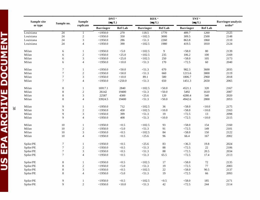
38

Sample site or type


Sample no.

24 24 24 24

Sample replicate

1 2 3 4

DNT a

(mmg/L)

Barringer Ref Lab

<1950.0 270 <1950.0 350 <1950.0 286 <1950.0 390

RDX a

(mmg/L)

Barringer Ref Lab

118.5 1770 <102.5 3000 <51.3 2260 <102.5 1980

TNT a

(mmg/L)

Barringer Ref Lab

489.7 1260 309.5 2500 863.8 1860 419.5 1810


2125 2148 2110 2124


6 6 6 6

1 2 3 4

<1950.0 <1950.0 <1950.0 <1950.0

<5.0 <25.0 <25.0 <10.0

<102.5 <102.5 <102.5 <51.3

9 235 250 170

<58.0 106.2 <58.0 <72.5

80 100 105 60

2139 2169 2173 2040


7 7 7 7

1 2 3 4

<1950.0 <1950.0 <1950.0 <1950.0

<50.0 <50.0 <10.0 <250.0

<51.3 <51.3 89.1

<51.3

670 660 580 650

982.3 1215.6 1806.7 1451.3

3600 3800 2960 2650

2035 2119 2018 2065


8 8 8 8

1 2 3 4

16917.1 26142 22587

33924.5

2840 19400 4300 19400

<102.5 <51.3 <25.6 <51.3

<50.0 <50.0 120

<50.0

4521.1 5492

4280.4 4942.6

320 1610 540 2800

2167 2087 2020 2053


9 9 9 9

1 2 3 4

<1950.0 <1950.0 <1950.0 <1950.0

712 450 399 408

<102.5 <102.5 <51.3 <51.3

36 <10.0

19 <10.0

<58.0 <58.0 <72.5 <72.5

<10.0 <10.0

13 <10.0

2175 2163 2098 2115


10 10 10 10

1 2 3 4

<1950.0 <1950.0 <1950.0 <1950.0

<0.5 <5.0 <0.5 <0.5

<102.5 <51.3 <102.5 <25.6

93 91 84 96

<58.0 <72.5 <58.0 66.4

154 149 150 167

2160 2101 2122 2002


7 7 7 7

1 2 3 4

<1950.0 <1950.0 <1950.0 <1950.0

<0.5 <0.5 <0.5 <0.5

<25.6 <51.3 <51.3 <51.3

83 88 88

65.5

<36.3 <72.5 <72.5 <72.5

19.8 22

20.5 17.4

2024 2106 2034 2113


8 8 8 8

1 2 3 4

<1950.0 <1950.0 <1950.0 <1950.0

<0.5 <5.0 <0.5 <5.0

<102.5 <51.3 <102.5 <51.3

17 19 22 19

<58.0 <72.5 <58.0 <72.5

72 77

90.5 66

2135 2083 2137 2093

Spike/PE Spike/PE

9 9

1 2

<1950.0 <1950.0

<0.5 <10.0

<102.5 <51.3

<0.5 42

<58.0 <72.5

185 244

2171 2114

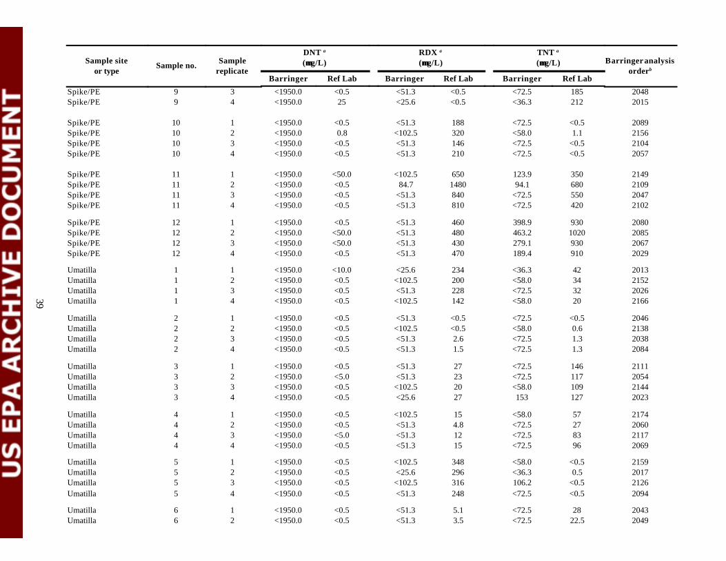
39

Sample site or type

Sample no. Sample replicate

DNT a

(mmg/L)

Barringer Ref Lab

RDX a

(mmg/L)

Barringer Ref Lab

TNT a

(mmg/L)

Barringer Ref Lab


Spike/PE Spike/PE

9 9

3 4

<1950.0 <1950.0

<0.5 25

<51.3 <25.6

<0.5 <0.5

<72.5 <36.3

185 212

2048 2015


10 10 10 10

1 2 3 4

<1950.0 <1950.0 <1950.0 <1950.0

<0.5 0.8

<0.5 <0.5

<51.3 <102.5 <51.3 <51.3

188 320 146 210

<72.5 <58.0 <72.5 <72.5

<0.5 1.1

<0.5 <0.5

2089 2156 2104 2057


11 11 11 11

1 2 3 4

<1950.0 <1950.0 <1950.0 <1950.0

<50.0 <0.5 <0.5 <0.5

<102.5 84.7

<51.3 <51.3

650 1480 840 810

123.9 94.1

<72.5 <72.5

350 680 550 420

2149 2109 2047 2102


12 12 12 12

1 2 3 4

<1950.0 <1950.0 <1950.0 <1950.0

<0.5 <50.0 <50.0 <0.5

<51.3 <51.3 <51.3 <51.3

460 480 430 470

398.9 463.2 279.1 189.4

930 1020 930 910

2080 2085 2067 2029

Umatilla Umatilla Umatilla Umatilla

1 1 1 1

1 2 3 4

<1950.0 <1950.0 <1950.0 <1950.0

<10.0 <0.5 <0.5 <0.5

<25.6 <102.5 <51.3 <102.5

234 200 228 142

<36.3 <58.0 <72.5 <58.0

42 34 32 20

2013 2152 2026 2166


2 2 2 2

1 2 3 4

<1950.0 <1950.0 <1950.0 <1950.0

<0.5 <0.5 <0.5 <0.5

<51.3 <102.5 <51.3 <51.3

<0.5 <0.5 2.6 1.5

<72.5 <58.0 <72.5 <72.5

<0.5 0.6 1.3 1.3

2046 2138 2038 2084


3 3 3 3

1 2 3 4

<1950.0 <1950.0 <1950.0 <1950.0

<0.5 <5.0 <0.5 <0.5

<51.3 <51.3 <102.5 <25.6

27 23 20 27

<72.5 <72.5 <58.0 153

146 117 109 127

2111 2054 2144 2023


4 4 4 4

1 2 3 4

<1950.0 <1950.0 <1950.0 <1950.0

<0.5 <0.5 <5.0 <0.5

<102.5 <51.3 <51.3 <51.3

15 4.8 12 15

<58.0 <72.5 <72.5 <72.5

57 27 83 96

2174 2060 2117 2069


5 5 5 5

1 2 3 4

<1950.0 <1950.0 <1950.0 <1950.0

<0.5 <0.5 <0.5 <0.5

<102.5 <25.6 <102.5 <51.3

348 296 316 248

<58.0 <36.3 106.2 <72.5

<0.5 0.5

<0.5 <0.5

2159 2017 2126 2094

Umatilla Umatilla

6 6

1 2

<1950.0 <1950.0

<0.5 <0.5

<51.3 <51.3

5.1 3.5

<72.5 <72.5

28 22.5

2043 2049

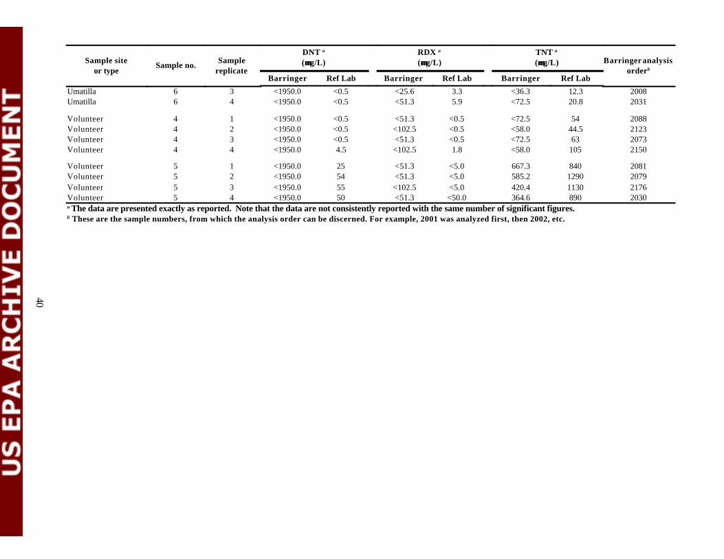
DNT a RDX a TNT a

Sample site Sample no. Sample (mmg/L) (mmg/L) (mmg/L) Barringer analysis or type replicate orderb

Barringer Ref Lab Barringer Ref Lab Barringer Ref Lab

Umatilla 6 3 <1950.0 <0.5 <25.6 3.3 <36.3 12.3 2008Umatilla 6 4 <1950.0 <0.5 <51.3 5.9 <72.5 20.8 2031

Volunteer 4 1 <1950.0 <0.5 <51.3 <0.5 <72.5 54 2088 Volunteer 4 2 <1950.0 <0.5 <102.5 <0.5 <58.0 44.5 2123 Volunteer 4 3 <1950.0 <0.5 <51.3 <0.5 <72.5 63 2073 Volunteer 4 4 <1950.0 4.5 <102.5 1.8 <58.0 105 2150

Volunteer 5 1 <1950.0 25 <51.3 <5.0 667.3 840 2081 Volunteer 5 2 <1950.0 54 <51.3 <5.0 585.2 1290 2079 Volunteer 5 3 <1950.0 55 <102.5 <5.0 420.4 1130 2176 Volunteer 5 4 <1950.0 50 <51.3 <50.0 364.6 890 2030 a The data are presented exactly as reported. Note that the data are not consistently reported with the same number of significant figures. b These are the sample numbers, from which the analysis order can be discerned. For example, 2001 was analyzed first, then 2002, etc.

40

Documents

Explosives Detection Technology Barringer Instruments … · summary of the test results for Barringer Instruments’ GC-IONSCAN™. This verification was conducted jointly with the