Exploring the Weak Limit of Gravity at Solar System Scales A dissertation submitted in partial

Exploring the Weak Limit of Gravity at Solar System Scales

A dissertation submitted in partial fulfillment of the requirements for the degree ofDoctor of Philosophy at George Mason University

By

Gary L. Page

Master of Business AdministrationVirginia Polytechnic Institute and State University, 1982

Master of ScienceClarkson University, 1971

Bachelor of ScienceClarkson University, 1969

Director: Dr. John F. Wallin, Associate ProfessorDepartment of Computational and Data Sciences

Spring Semester 2009George Mason University

Fairfax, VA

Copyright c© 2009 by Gary L. PageAll Rights Reserved

ii

Dedication

First and foremost, I dedicate this dissertation to my bride, Vicky, who encouraged me tobegin this journey and then steadfastly continued to provide support and assistance through-out the whole process. Thanks are due also to our children, Kelly and Amanda Wolcott,whose support and interest made the work much easier. Finally, my mother, Rose, and mylate father, Louis, provided an environment throughout my youth that encouraged curiosityand learning, and thus contributed directly towards my desire and ability to accomplish theeffort described here. Without all these people, the work would not have been possible andI dedicate the results to them.

iii

Acknowledgments

Dr. John Wallin could not have provided more help and guidance than he so ably andwillingly bestowed as my Dissertation Director. As a knowledgeable, flexible, and patientmentor and friend, I could not have asked for more, even though he had an annoyinghabit of being correct when we disagreed on technical matters. I also acknowledge thehelp, support, and assistance of the rest of my committee, Drs. Peter Becker, Kirk Borne,and Daniel Carr, who all provided assistance in various ways at various times and theirvaluable contributions are gratefully recognized. Additionally, thanks are due David Dixon,colleague, collaborator, friend, discoverer of asteroids, proprietor of Jornada Observatory(IAU 715), and expert in practical astrometry for providing both illuminating conversationsand periodic exhortations. Finally, I want to thank Dr. Barbara L. O’Kane, my associate,colleague, and friend from my “other life,” who provided support and assistance in manyways and at many times as the work proceeded.

iv

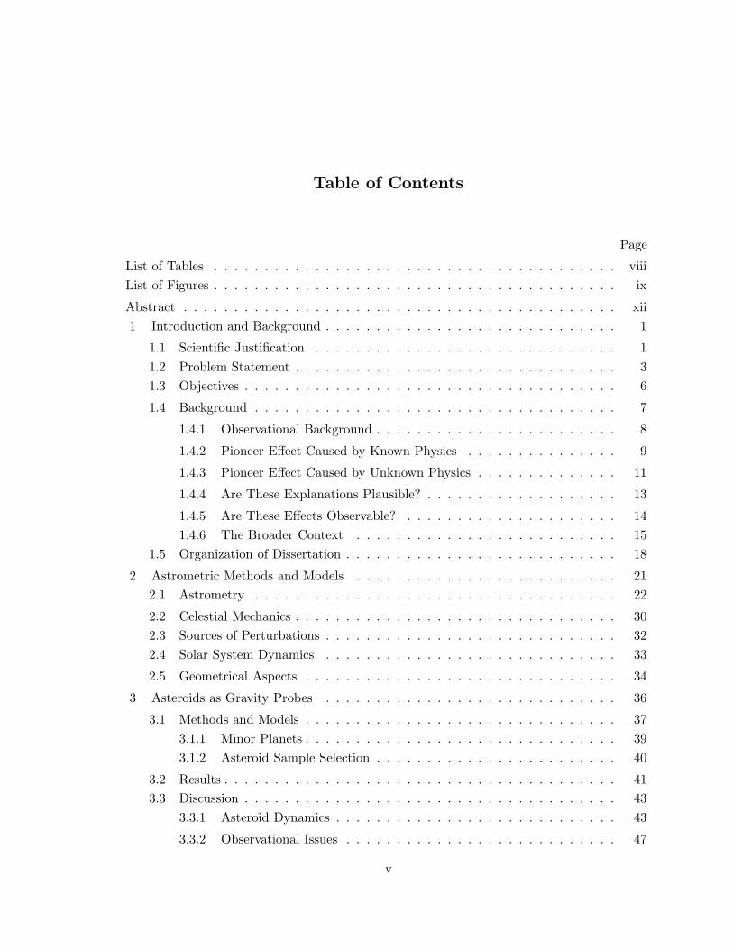
Table of Contents

Page

List of Tables . . . . . . . . . . . . . . . . . . . . . . . . . . . . . . . . . . . . . . . . viii

List of Figures . . . . . . . . . . . . . . . . . . . . . . . . . . . . . . . . . . . . . . . . ix

Abstract . . . . . . . . . . . . . . . . . . . . . . . . . . . . . . . . . . . . . . . . . . . xii

1 Introduction and Background . . . . . . . . . . . . . . . . . . . . . . . . . . . . . 1

1.1 Scientific Justification . . . . . . . . . . . . . . . . . . . . . . . . . . . . . . 1

1.2 Problem Statement . . . . . . . . . . . . . . . . . . . . . . . . . . . . . . . . 3

1.3 Objectives . . . . . . . . . . . . . . . . . . . . . . . . . . . . . . . . . . . . . 6

1.4 Background . . . . . . . . . . . . . . . . . . . . . . . . . . . . . . . . . . . . 7

1.4.1 Observational Background . . . . . . . . . . . . . . . . . . . . . . . . 8

1.4.2 Pioneer Effect Caused by Known Physics . . . . . . . . . . . . . . . 9

1.4.3 Pioneer Effect Caused by Unknown Physics . . . . . . . . . . . . . . 11

1.4.4 Are These Explanations Plausible? . . . . . . . . . . . . . . . . . . . 13

1.4.5 Are These Effects Observable? . . . . . . . . . . . . . . . . . . . . . 14

1.4.6 The Broader Context . . . . . . . . . . . . . . . . . . . . . . . . . . 15

1.5 Organization of Dissertation . . . . . . . . . . . . . . . . . . . . . . . . . . . 18

2 Astrometric Methods and Models . . . . . . . . . . . . . . . . . . . . . . . . . . 21

2.1 Astrometry . . . . . . . . . . . . . . . . . . . . . . . . . . . . . . . . . . . . 22

2.2 Celestial Mechanics . . . . . . . . . . . . . . . . . . . . . . . . . . . . . . . . 30

2.3 Sources of Perturbations . . . . . . . . . . . . . . . . . . . . . . . . . . . . . 32

2.4 Solar System Dynamics . . . . . . . . . . . . . . . . . . . . . . . . . . . . . 33

2.5 Geometrical Aspects . . . . . . . . . . . . . . . . . . . . . . . . . . . . . . . 34

3 Asteroids as Gravity Probes . . . . . . . . . . . . . . . . . . . . . . . . . . . . . 36

3.1 Methods and Models . . . . . . . . . . . . . . . . . . . . . . . . . . . . . . . 37

3.1.1 Minor Planets . . . . . . . . . . . . . . . . . . . . . . . . . . . . . . . 39

3.1.2 Asteroid Sample Selection . . . . . . . . . . . . . . . . . . . . . . . . 40

3.2 Results . . . . . . . . . . . . . . . . . . . . . . . . . . . . . . . . . . . . . . . 41

3.3 Discussion . . . . . . . . . . . . . . . . . . . . . . . . . . . . . . . . . . . . . 43

3.3.1 Asteroid Dynamics . . . . . . . . . . . . . . . . . . . . . . . . . . . . 43

3.3.2 Observational Issues . . . . . . . . . . . . . . . . . . . . . . . . . . . 47

v

3.4 Conclusions . . . . . . . . . . . . . . . . . . . . . . . . . . . . . . . . . . . . 57

4 Major Planets as Gravity Probes . . . . . . . . . . . . . . . . . . . . . . . . . . . 60


4.1.1 Characterizing the Pioneer effect . . . . . . . . . . . . . . . . . . . . 63

4.1.2 Estimating Pioneer effect manifestations . . . . . . . . . . . . . . . . 63

4.1.3 Celestial mechanics . . . . . . . . . . . . . . . . . . . . . . . . . . . . 65

4.1.4 Simulation of observations . . . . . . . . . . . . . . . . . . . . . . . . 68

4.2 Results . . . . . . . . . . . . . . . . . . . . . . . . . . . . . . . . . . . . . . . 73

4.2.1 Prediction of sky position from orbital elements . . . . . . . . . . . . 73

4.2.2 Errors in orbital elements derived from observations . . . . . . . . . 90

4.2.3 How can we assess the quality of an orbital fit? . . . . . . . . . . . . 96

4.3 Discussion . . . . . . . . . . . . . . . . . . . . . . . . . . . . . . . . . . . . . 100

4.4 Conclusions . . . . . . . . . . . . . . . . . . . . . . . . . . . . . . . . . . . . 103

5 Comets as Gravity Probes . . . . . . . . . . . . . . . . . . . . . . . . . . . . . . . 105


5.1.1 Non-Gravitational Forces . . . . . . . . . . . . . . . . . . . . . . . . 107

5.1.2 Comet Sample Selection . . . . . . . . . . . . . . . . . . . . . . . . . 107

5.2 Results . . . . . . . . . . . . . . . . . . . . . . . . . . . . . . . . . . . . . . . 108

5.3 Discussion . . . . . . . . . . . . . . . . . . . . . . . . . . . . . . . . . . . . . 111

5.4 Conclusions . . . . . . . . . . . . . . . . . . . . . . . . . . . . . . . . . . . . 116

6 Impact of LSST and Pan-STARRS . . . . . . . . . . . . . . . . . . . . . . . . . . 118


6.2 Results . . . . . . . . . . . . . . . . . . . . . . . . . . . . . . . . . . . . . . . 124

6.2.1 Angular Separation . . . . . . . . . . . . . . . . . . . . . . . . . . . . 124

6.2.2 Probability of a Significant Position Difference . . . . . . . . . . . . 128

6.2.3 Quality of Orbital Fits . . . . . . . . . . . . . . . . . . . . . . . . . . 131

6.3 Discussion . . . . . . . . . . . . . . . . . . . . . . . . . . . . . . . . . . . . . 136

6.3.1 Heuristic for Detection Times . . . . . . . . . . . . . . . . . . . . . . 136

6.3.2 Physical Basis for Heuristic . . . . . . . . . . . . . . . . . . . . . . . 141

6.3.3 What Would An Observer See? . . . . . . . . . . . . . . . . . . . . . 142

6.4 Conclusions . . . . . . . . . . . . . . . . . . . . . . . . . . . . . . . . . . . . 148

7 Astrometry Summary . . . . . . . . . . . . . . . . . . . . . . . . . . . . . . . . . 151

7.1 Discussion . . . . . . . . . . . . . . . . . . . . . . . . . . . . . . . . . . . . . 152

7.2 Conclusions . . . . . . . . . . . . . . . . . . . . . . . . . . . . . . . . . . . . 154

8 Dark Matter Methods and Models . . . . . . . . . . . . . . . . . . . . . . . . . . 161

8.1 Galactic Dark Matter Distribution . . . . . . . . . . . . . . . . . . . . . . . 161

8.2 Local Dark Matter Density . . . . . . . . . . . . . . . . . . . . . . . . . . . 164

vi

9 Dark Matter Capture Via a Weak Interaction . . . . . . . . . . . . . . . . . . . . 165


9.1.1 Solar Interior Model . . . . . . . . . . . . . . . . . . . . . . . . . . . 167

9.1.2 Solar Potential . . . . . . . . . . . . . . . . . . . . . . . . . . . . . . 170

9.1.3 Hard Sphere Scattering . . . . . . . . . . . . . . . . . . . . . . . . . 172

9.1.4 Scattering Cross Section . . . . . . . . . . . . . . . . . . . . . . . . . 173

9.1.5 Scattering Depth . . . . . . . . . . . . . . . . . . . . . . . . . . . . . 174

9.2 Results . . . . . . . . . . . . . . . . . . . . . . . . . . . . . . . . . . . . . . . 175

9.3 Discussion . . . . . . . . . . . . . . . . . . . . . . . . . . . . . . . . . . . . . 179

9.4 Conclusions . . . . . . . . . . . . . . . . . . . . . . . . . . . . . . . . . . . . 181

10 Dark Matter Capture Via Three-Body Interactions . . . . . . . . . . . . . . . . . 187


10.1.1 The Circular Restricted Three Body Problem . . . . . . . . . . . . . 189

10.1.2 Hill’s Problem . . . . . . . . . . . . . . . . . . . . . . . . . . . . . . 193

10.1.3 Curves of Zero Velocity . . . . . . . . . . . . . . . . . . . . . . . . . 196

10.2 Results . . . . . . . . . . . . . . . . . . . . . . . . . . . . . . . . . . . . . . . 198

10.3 Discussion . . . . . . . . . . . . . . . . . . . . . . . . . . . . . . . . . . . . . 203

10.4 Conclusions . . . . . . . . . . . . . . . . . . . . . . . . . . . . . . . . . . . . 204

11 Dark Matter Summary . . . . . . . . . . . . . . . . . . . . . . . . . . . . . . . . 207

11.1 Discussion . . . . . . . . . . . . . . . . . . . . . . . . . . . . . . . . . . . . . 208

11.2 Conclusions . . . . . . . . . . . . . . . . . . . . . . . . . . . . . . . . . . . . 210

12 Conclusions and Final Comments . . . . . . . . . . . . . . . . . . . . . . . . . . 213

12.1 Conclusions . . . . . . . . . . . . . . . . . . . . . . . . . . . . . . . . . . . . 213

12.1.1 Astrometry . . . . . . . . . . . . . . . . . . . . . . . . . . . . . . . . 213

12.1.2 Dark Matter Capture . . . . . . . . . . . . . . . . . . . . . . . . . . 217

12.2 Impact of Dissertation . . . . . . . . . . . . . . . . . . . . . . . . . . . . . . 218

12.3 Future Research Areas . . . . . . . . . . . . . . . . . . . . . . . . . . . . . . 220

12.4 Final Remarks . . . . . . . . . . . . . . . . . . . . . . . . . . . . . . . . . . 222

Bibliography . . . . . . . . . . . . . . . . . . . . . . . . . . . . . . . . . . . . . . . . . 224

vii

List of Tables

Table Page

1.1 Implications of the existence or nonexistence of the Pioneer effect and dark

matter. . . . . . . . . . . . . . . . . . . . . . . . . . . . . . . . . . . . . . . 16

3.1 Orbital parameters of asteroids susceptible to the Pioneer effect. . . . . . . 42

3.2 Observational characteristics of asteroid candidates on 2005 April 1. . . . . 45

4.1 Elements for the hypothetical bodies used in the analysis. . . . . . . . . . . 69

4.2 Frequency of archive observations of Pluto. . . . . . . . . . . . . . . . . . . 70

4.3 Total number of synthetic observations used in analysis, for each arc segment

evaluated. . . . . . . . . . . . . . . . . . . . . . . . . . . . . . . . . . . . . . 71

4.4 Four cases combining gravity models and forces determining motion. . . . . 72

5.1 Orbital parameters of comets susceptible to the Pioneer Effect. . . . . . . . 108

5.2 Change in comet orbital period because of Pioneer Effect and NGF. . . . . 110

5.3 Observational characteristics of comet candidates on 2005 April 1. . . . . . 112

6.1 The mean (in years), standard deviation (in years), and rms residual (in

arcsec) for each case described by a semimajor axis and an eccentricity. . . 130

6.2 Heuristic parameter values for time to a statistically significant angular sep-

aration. . . . . . . . . . . . . . . . . . . . . . . . . . . . . . . . . . . . . . . 137

viii

List of Figures

Figure Page

2.1 Keplerian elements describe the shape, size, and orientation of orbits. . . . 24

3.1 Angular deviation between Keplerian and perturbed orbits . . . . . . . . . 46

3.2 Maximum observable distance versus absolute visual magnitude . . . . . . . 47

3.3 Angular differences between positions of (5335) Damocles . . . . . . . . . . 51

3.4 Orbital fit rms residuals for Damocles . . . . . . . . . . . . . . . . . . . . . 55

4.1 Angular position differences when orbits are extrapolated with “known” el-

ements with– and without a Pioneer effect perturbation. . . . . . . . . . . . 74

4.2 Angular position difference when orbits are extrapolated with elements de-

termined from synthetic observations generated with a Pioneer effect pertur-

bation over a 50 year arc. . . . . . . . . . . . . . . . . . . . . . . . . . . . . 76













4.7 Angular position differences for Pluto when orbits are predicted with elements

determined from synthetic observations generated with a Pioneer effect per-

turbation. . . . . . . . . . . . . . . . . . . . . . . . . . . . . . . . . . . . . . 83

4.8 Observed minus calculated residuals for Pluto with respect to the DE414

ephemeris. . . . . . . . . . . . . . . . . . . . . . . . . . . . . . . . . . . . . . 85

ix

4.9 Normal points for the DE414 residuals and the residuals for the synthetic

observations relative to their ephemeris. . . . . . . . . . . . . . . . . . . . . 86

4.10 Total rms residual by epoch for the DE414 case and the synthetic observation

case. . . . . . . . . . . . . . . . . . . . . . . . . . . . . . . . . . . . . . . . . 89

4.11 The condition number of the orbital fitting problem as a function of eccen-

tricity for different observation arc lengths. . . . . . . . . . . . . . . . . . . 94

4.12 Relative error in orbital elements in the linear approximation as observation

arc varies. . . . . . . . . . . . . . . . . . . . . . . . . . . . . . . . . . . . . . 95

4.13 Rms residual of orbital fit as observation arc length varies. . . . . . . . . . . 98

4.14 Gravitational acceleration exerted by Uranus and Neptune on Pluto as a

function of time. . . . . . . . . . . . . . . . . . . . . . . . . . . . . . . . . . 101

5.1 Angular deviation between modified comet orbits. . . . . . . . . . . . . . . 114

6.1 Angular separation as a function of time from perihelion for an object with

a semimajor axis of 20 AU. . . . . . . . . . . . . . . . . . . . . . . . . . . . 125

6.2 Angular separation as a function of time from perihelion for an object with

a semimajor axis of 40 AU. . . . . . . . . . . . . . . . . . . . . . . . . . . . 127

6.3 Probability of a statistically significant angular difference as a function of

time from perihelion for an object with a semimajor axis of 20 AU. . . . . . 129

6.4 Probability of a statistically significant angular difference as a function of

time from perihelion for an object with a semimajor axis of 40 AU. . . . . . 129

6.5 Probability of a significant sky position difference between the perturbed and

the unperturbed case for selected objects as a function of time from perihelion.132

6.6 Rms residual for various combinations of observations and gravity model as

the observation arc lengthens. . . . . . . . . . . . . . . . . . . . . . . . . . . 134

6.7 Time (in years) from perihelion that gives a 95 percent probability of a signifi-

cant difference in sky position between a perturbed case and the unperturbed

case. . . . . . . . . . . . . . . . . . . . . . . . . . . . . . . . . . . . . . . . . 138

6.8 Time for an object that sometimes comes within 20 AU of the Sun to reach

a significant angular separation. . . . . . . . . . . . . . . . . . . . . . . . . . 140

6.9 True anomaly at which an observable position difference between the per-

turbed and unperturbed cases is found at the 95 percent significance level. . 142

6.10 True anomaly that results in observable positional differences at the 95 per-

cent significance level. . . . . . . . . . . . . . . . . . . . . . . . . . . . . . . 143

6.11 Normal points in right ascension for an object with a semimajor axis of 25

AU and an eccentricity of 0.3 in a “matching” case. . . . . . . . . . . . . . . 146

x

6.12 Normal points in right ascension for an object with a semimajor axis of 25

AU and an eccentricity of 0.3 in a “mismatched” case. . . . . . . . . . . . . 147

9.1 Solar mass interior to a radial distance . . . . . . . . . . . . . . . . . . . . . 168

9.2 Solar temperature versus radial distance . . . . . . . . . . . . . . . . . . . . 168

9.3 Total mass density versus radial distance . . . . . . . . . . . . . . . . . . . . 169

9.4 Mass fraction of main Solar constituents versus radial distance . . . . . . . 169

9.5 Gravitational potential energy per unit mass inside the Sun . . . . . . . . . 172

9.6 Illustrative dark matter trajectories through the Sun . . . . . . . . . . . . . 176

9.7 Optical depth to scattering for two dark matter trajectories . . . . . . . . . 177

9.8 Number of dark matter particles suffering different fates as dark matter par-

ticle mass varies . . . . . . . . . . . . . . . . . . . . . . . . . . . . . . . . . 179

9.9 Log of binned frequency of captured dark matter particles as dark matter

mass is varied . . . . . . . . . . . . . . . . . . . . . . . . . . . . . . . . . . . 180

9.10 Frequency of energy bins of captured dark matter particles . . . . . . . . . 181

9.11 Frequency of semimajor axis bins for captured dark matter . . . . . . . . . 182

9.12 Optical depth to scattering as a function of time for several representative

orbits . . . . . . . . . . . . . . . . . . . . . . . . . . . . . . . . . . . . . . . 184

9.13 Representative set of orbital states that a dark matter particle traverses from

initial capture into Solar orbit to eventual escape . . . . . . . . . . . . . . . 185

10.1 Zero velocity curves in the orbital plane of the primaries . . . . . . . . . . . 198

10.2 Zero velocity curves in the orbital plane of the primaries for different values

of CJ . . . . . . . . . . . . . . . . . . . . . . . . . . . . . . . . . . . . . . . . 200

10.3 Zero velocity curves for the Hill problem in the orbital plane of the primaries

for different values of CH . . . . . . . . . . . . . . . . . . . . . . . . . . . . 202

10.4 Zero velocity curves for the Hill problem in different planes for different values

of CH . . . . . . . . . . . . . . . . . . . . . . . . . . . . . . . . . . . . . . . 202

xi

Abstract

EXPLORING THE WEAK LIMIT OF GRAVITY AT SOLAR SYSTEM SCALES

Gary L. Page, PhD

George Mason University, 2009

Dissertation Director: Dr. John F. Wallin

Precision tracking of multiple spacecraft in the outer Solar System has shown an unmod-

elled perturbation, consisting of a small, constant, radial acceleration directed towards the

Sun. Since its detection, a great deal of work has been devoted to explaining this Pioneer

effect, both in terms of spacecraft-generated systematics and external physical causes. Its

continuing importance is found in the fact that it has been impossible to explain away the

effect through conventional means. This leaves open the possibility, however unlikely, that

new physics is represented in the effect. This new physics, in turn, would be connected

intimately to gravity with huge implications across astrophysics and beyond.

With this as motivation, this dissertation investigates two areas related to the Pioneer

effect. The first goal is to investigate the use of planets, comets, and asteroids to determine

the reality of the Pioneer effect through precision astrometry.

Here, we showed that asteroids can be used to evaluate the gravitational field in the

outer Solar System. The observations can be conducted with modest allocations of telescope

time, and would provide a definitive answer to the question within the next 20 years.

In assessing current knowledge of Pluto’s orbit, we determined that it is not known well

enough at present to preclude the existence of the Pioneer effect. We also showed that

comets are not ideal candidates for measuring gravity in the outer Solar System, although

some present intriguing observational targets for related reasons. Finally, we showed that

Pan-STARRS and LSST are likely to lead to a capability to test gravity in the outer Solar

System in the near future.

The second goal of the dissertation involved exploring two general mechanisms for ex-

plaining the Pioneer effect. The first approach involved investigating the effective mass

density that would be produced in the Solar System as a result of the capture of elementary

particle dark matter by means of a hypothetical weak interaction between the dark matter

particles and the matter of the Sun. The second approach involved three body capture of

dark matter from the Galactic halo into Solar orbit. The three bodies interacting are the

Galactic barycenter, the Sun, and the dark matter particle.

In this phase of the dissertation, we showed that capture of Galactic dark matter into

Solar orbit by a weak interaction with Solar matter does not accumulate dark matter in

the region where the Pioneer effect manifests itself. It is possible that it does accumulate

at smaller distances, however. Similarly, we showed that three body gravitational capture

is not feasible as a cause of the Pioneer effect either. Dark matter captured by this mecha-

nism would occur generally at distances far greater than that needed to cause the Pioneer

anomaly. Thus, neither mechanism for capture of dark matter into Solar orbit sufficed to

explain the Pioneer effect.

Finally, we discuss a number of future research areas that became apparent during the

course of the research.

Chapter 1: Introduction and Background

This dissertation describes a research program that investigates the use of astrometry of

outer Solar System bodies as a probe of gravity at multiple AU scales. The effort is part of

a broader research program that includes investigation of Solar System capture scenarios

of Galactic dark matter that could have observable dynamical effects.

This line of research is important because gravity is the primary force molding the

evolution of the entire cosmos. Introducing ad hoc concepts like dark matter to make

theories fit observation follows a time-honored approach of assuming the basic correctness

of our picture of Nature and adding the simplest concepts necessary to make our picture

whole. Many times in the past, the reality of the new concepts was eventually demonstrated.

However, given the lack of success in directly detecting dark matter and having no empirical

basis for even speculating on its nature, the time has come to investigate other possibilities.

1.1 Scientific Justification

While at first glance the goal of investigating the weak limit of gravity at Solar System

scales might seem to be a settled problem, the reality is quite different. At laboratory

scales, Newton’s Law of Universal Gravitation is experimentally verified by such means as

the Cavendish experiment and its variants and descendants. At the distance scale of the

inner planets, the tracking of space probes has experimentally confirmed our modern un-

derstanding of gravity to a high degree of accuracy. This is especially true for Venus, Mars,

the Moon, and, of course, our own planet, whose positions in space have been essentially

“surveyed in” by multiple spacecraft.

At the largest scale, that of galaxy clusters, we observe gravitational lensing of distant

galaxies by foreground clusters. However, we do not see enough matter to provide the

1

requisite mass to cause the lens. Similarly, on somewhat smaller but still large scales,

the rotation curves of individual galaxies cannot be understood in terms of rotation in a

gravitational field produced by the visible matter. In facing these issues, investigators had

two choices. Either they could assume that there was some invisible matter influencing the

motion, or that our theories of gravity were wrong. Normally, the easy way out is to assume

that dark matter exists, even though we have no real idea of its nature and have not yet

succeeded in directly detecting it.

At intermediate scales, say that of binary stars, we have problems observationally veri-

fying our understanding of gravity. Such objects have only been known for about 200 years

and long period binaries are not even known to be gravitationally bound to one another.

Even shorter period binaries have not been studied extensively enough to observe deviations

from normal gravity. Note that, as our interest is in weak-field systems, in this discussion we

are ignoring binary pulsars and close, relativistic binaries, where gravity is well-measured

by, for example, pulsar timings.

At somewhat smaller spatial scales, we have the outer planets of our Solar System

along with various minor planets, comets, etc. The question addressed in this dissertation

and our research program is whether gravity can be tested at the 20 to 100 AU distance

scales typical of our local environment. Even at these scales, there is some evidence of

“problems” with gravity. Our most precisely tracked spacecraft, Pioneers 10 and 11, have

shown a constant sunward radial acceleration (termed the Pioneer effect) over a range of

heliocentric distances from 20 to 75 AU that has resisted conventional explanation. Thus,

wherever we look at either very weak gravity fields or, perhaps the same thing, at large

distances, we see problems with our understanding of gravity. This and related issues are

among the outstanding problems facing astronomy and astrophysics as we enter the twenty-

first century.

2

1.2 Problem Statement

As I will discuss below, a great deal of work has been devoted to explaining the Pioneer

effect, both in terms of spacecraft-generated systematics and external physical causes. The

importance of this is found in the fact that it has been impossible to explain away the

effect through conventional means. This leaves open the possibility, however unlikely, that

new physics is represented in the effect. This new physics, in turn, would be intimately

connected to gravity with huge implications across astrophysics and beyond.

Continuing professional interest in this area of research has been shown by the Euro-

pean Space Agency, as part of its Cosmic Vision 2015-2025 planning (Bignami et al., 2005),

exploring as a major theme “What are the fundamental physical laws of the Universe,” that

envisions high precision experiments in space aimed at uncovering new physics, including

probing the limits of general relativity, symmetry violations, etc. Further, the International

Space Science Institute has convened an international team, “The Pioneer Explorer Collab-

oration: Investigation of the Pioneer Anomaly at ISSI,”1 to define a process by which the

entire Pioneer data record can be analyzed and to use the results to define an instrument

package capable of providing an independent confirmation of the anomaly and to study the

feasibility of a dedicated mission to explore the Pioneer effect (Dittus et al., 2006).

Even continuing public interest in this area of research is shown by the fact that the

most successful fundraising appeal conducted to date by the Planetary Society has been to

support saving the complete record of all existing Pioneer tracking data, allowing continuing

efforts to analyze the complete dataset.

These efforts have borne fruit and an extended dataset has been successfully recovered.

It is being analyzed in a number of ways by a number of groups, and recent reports of

progress have appeared in the literature (List and Mullin, 2008; Toth and Turyshev, 2006,

2008; Turyshev and Toth, 2007; Turyshev et al., 2006, for example).

In light of the continuing interest in this problem, one primary goal of the dissertation

is to investigate the use of planets, comets, and asteroids to investigate the reality of the

1 http://www.issi.unibe.ch/teams/Pioneer

3

Pioneer effect. The proposed method of attack is one that has neither been tried nor

explored by interested parties.

Although theorists have explored many potential causes of the Pioneer effect, Occam’s

razor dictates that we preferentially investigate simpler explanations as a first choice. To

this end, the second phase of the dissertation involves exploring two general mechanisms

for explaining the Pioneer effect within the currently accepted astrophysical context.

The first approach involves investigating the effective mass density that would be pro-

duced in the Solar System as a result of the capture of elementary particle dark matter

by means of a hypothetical weak interaction between the dark matter particles and the

matter of the Sun. This approach is restricted to potential dark matter candidates such as

neutrinos or more exotic particles like neutralinos or axions that are able to interact weakly

with matter in the interior of the Sun.

The second approach to explaining the Pioneer effect involves an effect that has not

heretofore been recognized: three body capture of dark matter from the Galactic halo into

Solar orbit. We are all familiar with utilizing gravity assist trajectories to minimize travel

time for spacecraft on the way to the outer planets. What hasn’t previously been explored

is using this same dynamical phenomenon in reverse. In this case the three bodies whose

interactions can cause halo dark matter to lose sufficient energy to become bound to the

sun are the Sun itself, the dark matter particle, and the Galactic barycenter. The process

has a very large capture cross section and has the additional benefit of applying to any

dark matter candidate (either elementary particle or macroscopic bodies of various levels

of exoticness).

Summarizing, the problem areas addressed in the dissertation are twofold:

• Investigating the feasibility of using major and minor planets to investigate gravity

at intermediate scales and in particular to evaluate the reality of the Pioneer effect.

• Investigating several potential causes of gravitational perturbations due to dark matter

in the outer Solar System, and through them the Pioneer effect.

4

The importance of this effort lies in its relation to empirically investigating the weak

limit of gravity at Solar System scales. This is an outstanding problem that, in turn,

ties into perhaps one of the largest problems outstanding in astrophysics—the nature and

existence of dark matter.

As far as the first problem area is concerned, it is a remarkable fact that once minor

planets are discovered and their orbits determined, there is little follow-up on characterizing

their orbits if they are found to present no earth impact threat. Minor planets are never

followed with an eye towards assessing the gravitational fields through which they travel.

Indeed, many asteroids are currently “lost” in that it has been so long since any reported

observations were made that they could not now be observed by looking in a predicted

position—a new search would be required (Sansaturio et al., 1998).

The orbits of the outer planets are well modeled, even though there remain irritating

discrepancies in the residuals of Pluto. However, in the absence of extended visits by

spacecraft, there remain uncertainties in the orbital elements of the outer planets that

could easily obscure small perturbations like the Pioneer effect. Thus, there are few tests

of gravity at intermediate distance scales and theorists considering gravity at these scales

are operating in an empirical vacuum.

There is even disagreement about the degree to which observations of the outer planets

validate Newtonian gravity (Krotkov and Dicke, 1959). Indeed, recently Page et al. (2006)

stated that observational uncertainties associated with the positions of the outer planets

make them infeasible for demonstrating or refuting the existence of the Pioneer effect. This

statement resulted in several citations that disputed that assertion (Iorio and Giudice, 2006;

Tangen, 2007), or at least to assert that the statement is controversial (Sanders, 2006). The

issues raised by these researchers are dealt with elsewhere in the dissertation.

In any case, if a method of measuring the Pioneer effect was available it might serve,

once and for all, to either support or refute its existence as a real phenomenon. Depending

upon the characteristics of the measurements, it might even be possible to differentiate

between alternative predictions of different explanations for the effect.

5

Thus, one main purpose of the dissertation is to outline the feasibility of using obser-

vations of planets, comets, and asteroids to evaluate the distribution of mass in the outer

Solar System and thereby explore the Pioneer effect by precision astrometry. Secondly, its

purpose is to evaluate some possible causes of the Pioneer effect and whether they are ob-

servationally detectable. Such a program could have profound effects on our understanding

of the mass distribution in the outer Solar System.

1.3 Objectives

Within the two broad purposes outlined above, the main objectives of the dissertation

include the following:

• Using asteroids to measure the Pioneer effect—This objective involves investigating

whether asteroids can be used to determine whether or not the Pioneer effect can be

validated by means of astrometric observations. The work shows that a sustained

observation campaign or properly chosen asteroids can over time show whether or not

the Pioneer effect exists.

• Using major planets as a probe of gravity in the outer Solar System—Contrary to a

number of statements in the literature, and in agreement with other assertions I have

made, we show that the motion of the major outer planets do not indicate that the

Pioneer effect does not exist; rather, uncertainties in the orbit of Pluto potentially

conceal small perturbations to gravity.

• Using comets to measure the Pioneer effect—This objective seeks to investigate the use

of comets to see if they provide a vehicle for measuring the Pioneer effect. As smaller

and typically fainter bodies that are also subject to nongravitational perturbations

(Marsden et al., 1973), comets are not ideal candidates for this purpose; however, the

general feasibility of comets in this role is the primary thrust of this objective.

• Exploring the impact of uncoming large, high observation cadence instruments such as

Pan-STARRS and LSST on the use of objects in the outer Solar System to investigate

6

gravity—Recognizing the scarcity of time on large telescopes, the dissertation shows

that the advent of high speed, deep surveys will revolutionize the use of minor planets

as probes of gravity in the outer Solar System.

• Evaluating mass capture due to particle interactions between dark matter and matter

in the Sun as a source of the Pioneer effect—If Galactic dark matter exists as ele-

mentary particles, and if it interacts both gravitationally and weakly with baryonic

matter, those interactions should lead to capture of dark matter into Solar orbit. The

thrust of this objective is to evaluate the possibility that dark matter captured in this

way can explain the Pioneer effect.

• Evaluating three-body capture as a mechanism for explaining the Pioneer effect—A

mechanism for explaining the Pioneer effect in the context of a mass concentration

in the outer Solar System that has not previously been investigated is through three-

body capture of Galactic dark matter into Solar orbit. In this context the three bodies

are the Galactic barycenter, the Sun, and the dark matter particle. Note that this

mechanism does not demand that dark matter be of an elementary particle nature.

Any type of dark matter that gravitates would be subject to this effect.

The dissertation outlined above, in addition to standing on its own in terms of originality

and scientific utility, is also open-ended in that it provides a natural path to future activities

in an open, but important, area of research: Assessing gravity at the multiple AU scale.

This area of research seems particularly fruitful and a number of potential future research

areas are clearly visible. These future directions are outlined later in the dissertation.

1.4 Background

As indicated above, our interests here are broader than whether or not the Pioneer effect

really exists. Rather, we are attempting to assess the weak limit of gravity at intermediate

scales like that of the Solar System. However, the Pioneer effect provides an empirical

touchstone upon which we can base our investigation. Below, we describe the Pioneer

7

effect in some detail, outlining potential explanations that have thus far failed to convince

researchers that they in fact explain the observations, discuss whether or not the explanation

attempts are plausible, and whether the Pioneer effect is independently verifiable. Finally,

we describe a somewhat broader view of the arena within which the dissertation operates,

and show that the researches described here have meaning, validity, and worth whether or

not the Pioneer effect really exists.

1.4.1 Observational Background

Beginning in 1972, humanity began exploring the outer Solar System with the launch of

Pioneer 10. As this probe receded from Earth and continued performing its initial and

extended missions, other robotic explorers followed in its wake. In 1973, Pioneer 11 was

launched; the twin spacecraft Voyager 1 and 2 both departed in 1977; Galileo left on its

roundabout trip in 1989; Ulysses was launched into a Solar polar orbit in 1990; Cassini

went on its way in 1997, and after passing by Jupiter, has entered orbit around Saturn for

its extended mission; and in 2006, New Horizons left to visit Pluto in 2015. During these

missions, a number of groups followed the probe’s trajectories with interest, attempting to

discern unexplained perturbations of various types in the motion of the spacecraft. Anderson

et al. (1989) placed bounds on the amount of dark matter in Solar orbit by using Voyager 2

Uranus flyby data to generate a new and more accurate ephemeris which bounded the extra

mass. This work was followed by Anderson et al. (1995), which used Voyager 2 Neptune

flyby data, coupled with data from the Jupiter encounters of Pioneer 10 and 11, as well as

Voyager 1 to improve the dark matter bounds derived previously.

The Pioneers were of particular interest in this regard. As “primitive” spacecraft, they

were spin stabilized and required a minimum number or Earth reorientation maneuvers

which permitted precise acceleration measurements. The Voyager probes, on the other

hand, were three axis stabilized and conducted numerous attitude control maneuvers that

overwhelmed the small signature of the anomalous acceleration. The Pioneer design is in

keeping with one of the main objectives of their extended missions, which was to conduct

8

accurate celestial mechanics measurements. However, both Galileo and Ulysses were also

investigated. The failure of Galileo’s high gain antenna to deploy made integration times for

data collection uncomfortably long, This, coupled with the closeness of the Sun and the size

of the spacecraft, made it very difficult to collect the necessary ranging data to determine the

position of the spacecraft and made it impossible to separate out Solar radiation effects from

any anomalous acceleration. Thus, Galileo data could not be used to verify the existence of

the anomaly. Ulysses, on the other hand, gives some indication of an anomalous acceleration,

but the assumptions required and the high correlation between Solar radiation forces and

any anomalous acceleration make it impossible to convincingly separate out the two effects.

The Pioneer probes are the primary focus here, and both following Pioneer 10’s Jupiter

encounter and Pioneer 11’s Saturn encounter, they continued outward on hyperbolic trajec-

tories, leaving the Solar System. Because of their spin-stabilization and large heliocentric

distances, they provided ideal platforms for their extended mission of conducting dynamical

studies of the outer Solar System.

As reported by Anderson et al. (1998), beginning in 1980 when Pioneer 10 was 20 AU

from the Sun and the pressure due to Solar radiation had decreased to less than 5×10−8 cm

sec−2, analysis of unmodeled accelerations found that the biggest systematic error in the

acceleration residuals was a constant acceleration, directed towards the Sun, of approximate

magnitude 8 × 10−8 cm sec−2, well in excess of the five day average acceleration accuracy

of 10−8 cm sec−2. When Pioneer 11 passed this 20 AU threshold, a similar effect was seen.

Prompted by this unusual result, Galileo and Ulysses data were investigated for a similar

effect. Although the limited data available from Galileo could not be used, Ulysses showed

a similar unmodeled acceleration residual, even at its much smaller heliocentric distance.

The effect on the Pioneers has persisted until at least a heliocentric distance of 75 AU.

1.4.2 Pioneer Effect Caused by Known Physics

As might be expected, the well-reasoned arguments for an anomalous acceleration in the

outer Solar System precipitated a large body of work in an effort to explain the acceleration

9

in terms not requiring additional hypothetical mass concentrations with special properties.

In a capstone paper, Anderson et al. (2002a) reviews and addresses a large number of

objections to the conclusion that there is an anomalous acceleration and provides a detailed

look at technical information on the Pioneers that was previously not readily available.

Roughly speaking, potential causes of the Pioneer effect can be divided into those imposed

upon the spacecraft from external sources, and those originating within the spacecraft.

Among the former are: Solar radiation pressure, wind, and corona; the stability of clocks

and the mechanical stability of the NASA Deep Space Network (DSN) antenna complex;

and electromagnetic Lorentz forces acting on a charged spacecraft. The latter encompass

reaction forces from the emitted radio beam, differential emissivities of the Radioisotope

Thermoelectric Generators (RTGs), helium expelled from the RTGs due to decay of their

plutonium fuel, and gas leaks.

Anderson et al. (2002a) also reviews a number of attempts to explain the Pioneer effect

in terms of known physics. These include: mass concentrations due to resonance effect with

Neptune and Pluto (Malhotra, 1995, 1996), forces due to a hypothetical disk of matter in

the ecliptic plane (Boss and Peale, 1976), and the implications for the Pioneer effect of

these concentrations (Liu et al., 1996). Similarly, RTG heat reflecting off the spacecraft was

investigated (Anderson et al., 1999a; Katz, 1999) and non-isotropic radiative cooling of the

spacecraft was suggested (Anderson et al., 1999b; Murphy, 1999). Variations on this theme

were also suggested by Scheffer (2001a,b, 2003) and discussed in Anderson et al. (2001).

The idea that the Pioneer effect was due to some new manifestation of known physics

was also explored. Anderson et al. (2002a), for example, also investigated the feasibility of

the anomalous acceleration being due to some unknown interaction of radio signals with

the Solar wind. Similarly, Crawford (1999) investigated the idea of a gravitational red shift

causing the Pioneer effect. Others looked at resistance to the motion of the spacecraft due

to interplanetary dust, but infrared observations ruled out dust as a cause (Backman et al.,

1995; Teplitz et al., 1999).

Investigation of these areas continues. In particular, Nieto (2005) analytically assessed

10

the possiblity that Kuiper Belt mass distributions could lead to the Pioneer effect. Similary,

Xu and Siegel (2008) and Peter and Tremaine (2008) investigated the mass distribution in

the Solar System of dark matter particles being captured by means of three body interactions

between the Sun, planets, and the dark matter particles. Additionally, the ongoing analysis

of the extended Pioneer dataset has led to further investigation of thermal issues with the

spacecraft (Bertolami et al., 2008; Toth and Turyshev, 2009) and the possiblity that thermal

radiation is the cause of the Pioneer effect.

None of these mechanisms convincingly explains the Pioneer effect. Although even

the discoverers of the Pioneer effect acknowledge that spacecraft systematics are the most

likely explanation for the acceleration, there have been no convincing arguments that that

is the case. The alternative, that the Pioneer effect represents a real phenomenon, is very

appealing for many reasons. What is lacking is a means of measuring the effect, its variation,

its potential anisotropies, and its region of influence.

The bottom line is that the Pioneer effect seems well-founded and has not been con-

vincingly explained in terms of known physics or engineering parameters of the spacecraft

involved. Although spacecraft systematics remain the most likely explanation for the Pio-

neer effect, its potential existence is of great interest for a variety of fundamental physical

reasons.

1.4.3 Pioneer Effect Caused by Unknown Physics

Anderson et al. (2002a) also reviews a large number of potential explanations for the anoma-

lous acceleration in terms of new physics. These include: whether the effect is due to dark

matter or a modification of gravity; whether it is a measure of space-time curvature and cos-

mological expansion (e.g., Solar System coordinates are not inertial coordinates); whether

it is due to a number of more radical variants on the relativistic gravity theme.

However, in the end, Anderson et al. (2002a) finds “no mechanism or theory that ex-

plains the anomalous acceleration.” Thus, in the minds of the authors of that paper, the

possibility of new physics could not be ruled out. Interest in the phenomenon continues.

11

For example, Anderson et al. (2002b) reports a potential consequence of a Pioneer effect on

the structure of the Oort cloud, and others attempt to explain the anomalous acceleration

as a manifestation of the cosmological constant (Nottale, 2003).

Some simple ideas that might seem to have potential for explaining the Pioneer effect

were explored in a different context. For example, Talmadge et al. (1988) investigated

the impact of a number of different gravitational alternatives (e.g., a different force law

exponent, a Yukawa-type distance dependence, and MOND2) and found that the motion of

the inner planets is known so precisely from space-based measurements, that none of these

alternatives are feasible as modifications to gravity.

Some additional ideas investigated include modifying gravity with a Yukawa-type cor-

rection term (Capozziello et al., 2001), long range accelerations induced by a new scalar

field (Mbelek and Lachieze-Rey, 1999), and conformal gravity with dynamic mass genera-

tion (Wood and Moreau, 2001). A hypothetical superstrong interaction between photons or

massive bodies and individual gravitons as a cause of a nondoppler cosmological red shift

was investigated (Ivanov, 2002), as were other possible manifestations of the graviton back-

ground (Ivanov, 2001). Cosmological models in 4+1 dimensions with a changing time scale

factor were evaluated in the context of the Pioneer effect (Belayev, 1999), as were the time

variation of the Newtonian gravitational constant (Mansouri et al., 1999). More recently,

deformation of planetary orbits by a time dependent gravitational potential in the universe

(Trencevski, 2005) and more exotic models have also been evaluated, including five dimen-

sional brane worlds, which might manifest corrections to Newtonian gravity (Bronnikov et

al., 2006).

Exotic proposal continue. Østvang (2002) investigated explaining the Pioneer effect with

“quasi-metric” relativity, Belayev and Tsipenyuk (2004) looked at gravi-electromagnetism

in five dimensions, Ranada (2004) sought an explanation in the acceleration of clocks, and

McCulloch (2007) modelled the Pioneer effect as modified inertia. Other ideas that were

2 MOdified Newtonian Dynamics, a Newtonian gravity alternative which can be viewed as positing a mini-

mum acceleration.

12

investigated include a variable cosmological constant and a test particle moving in a cloud

of dust (Massa, 2008), and the endless possiblities inherent in a rotating Godel universe

(Wilson, 2008).

The point made by this somewhat lengthy, but very incomplete, summary of research

into potential “new physics” explanations for the Pioneer effect is that it has generated no

shortage of ideas, many devoid of any connection with empiricism, to explain this intriguing

phenomenon.

1.4.4 Are These Explanations Plausible?

As observed above, even the discoverers of the Pioneer effect believe that spacecraft sys-

tematics are its most likely cause. The problem is that investigators have been unable to

agree that reasonable values of the systematics are large enough to provide the observed

effect. The prosaic explanations are all reasonable and plausible; they just don’t seem to

add up to enough thrust to cause the Pioneer effect.

There are a multitude of such systematic effects and not all are well understood. Indeed,

even if the Pioneer effect is shown convincingly to not exist as an independent effect and

is merely due to systematics, the probable outcome of such a finding is that it would be

recognized that greater care is needed in characterizing spacecraft destined for high precision

missions. This endeavor would be worthwhile to engineers and others on its own merits.

With respect to the “new physics” causes, we must note that “new physics” presents

itself to us very infrequently and must be dealt with using the strongest possible skepti-

cism. However, one must acknowledge that the payoff associated with “new physics” is

extraordinarily large and so we ignore exotic possibilities at our collective peril. Our entire

academic preparation is necessarily devoted to performing “standard science” rather than

the “new science” that is only very occasionally called for (Kuhn, 1996). Perhaps this is why

we all remember the pioneers of new areas even though those areas undergo great growth

in application and sophistication as time progresses, sometimes making the research areas

virtually unintelligible to their originators.

13

This dissertation provides two thrusts of fundamental importance. First, recognizing

that astrophysics is empirically based, we seek to develop an observational technique to ex-

plore the Pioneer effect. Certainly this approach is less expensive and easier than designing,

building, launching, and monitoring special purpose or piggyback space probes intended to

explore the Pioneer effect. At the very least these two approaches complement one another.

Secondly, this disertation will evaluate two less exotic possible explanations of the Pio-

neer effect that have not heretofore been investigated. Both of these approaches involve the

capture of dark matter into Solar orbit. In the first case, the underlying assumption is that

the dark matter consists of nonbaryonic elementary particles that interact with baryonic

matter through gravity (or else it would not suffice to be dark matter) and a hypothet-

ical weak interaction. The other approach involves three body capture into Solar orbit

which would operate against any matter, dark or otherwise, orbiting the Galaxy. Thus, this

capture process is more general and, since it involves only gravity, would operate against

any possible dark matter candidate ranging from elementary particles to brown dwarfs and

mini-black holes (Titarchuk and Chardonnet, 2006).

1.4.5 Are These Effects Observable?

As outlined elsewhere in the dissertation, the problem of the Pioneer effect and determining

if it is real or not can be attacked in a number of ways. The theorists have been going wild

offering many alternatives to general relativistic gravity and even non-Newtonian offshoots

like MOND. Additionally, possible explanations relating to cosmological expansion, time

variations, inertial effects, and even more exotic possibilities have been discussed at length

in the literature. Unfortunately, in all these cases, what is missing is empirical evidence

beyond the few Pioneer effect observations.

Another class of approaches involve spacecraft. The European Space Agency is con-

sidering both special purpose and piggyback spacecraft intended to explore the Pioneer

effect. The recently launched New Horizons probe to Pluto and beyond has a lengthy spin-

stabilized cruise phase after its gravity assist maneuver near Jupiter and, after leaving the

14

Jovian magnetospheric tail, tracking data will start being recorded for analysis some time

in the future when funding is available3 (see also Nieto, 2008). The distinguishing charac-

teristic of these approaches is that the very expensive and time consuming process of going

from mission formulation and planning to spacecraft construction and finally launch and

mission conduct. Indeed, the only probe (New Horizons) currently en route and able to

contribute to the understanding of the Pioneer effect does not have funds to support the

requisite analysis, although there is hope that they will be available in the future.

In this dissertation another approach is offered. First, we will investigate the use of

bodies in the outer Solar System to attempt to measure the Pioneer effect. Although this

approach is likely to require a long-term observation campaign, it is inexpensive and com-

plements potential space-based approaches. Secondly, we will investigate two alternative

causes of the Pioneer effect that have not elsewhere been evaluated. Both of these alter-

natives involve the capture of Galactic dark matter into Solar orbit and investigating the

potential for these processes to explain the Pioneer effect in terms of current physics. These

approaches are new in the context of the Pioneer effect and one approach, three-body cap-

ture, has the attractive feature that it operates on any type of dark matter that gravitates.

Of course, if dark matter doesn’t gravitate, it doesn’t satisfy the minimum requirements

for its invocation—explaining the rotation curves of galaxies and gravitational lensing by

clusters of galaxies.

1.4.6 The Broader Context

At first glance it might seem that the dissertation is heavily weighted towards, and highly

dependent upon, the existence of the Pioneer effect. We use the Pioneer effect as a not

currently understood empirical observation that is an exemplar of the type of gravitational

perturbation that could result from a lack of understanding of gravity at intermediate

distance scales. Because of this, the twin problem areas attacked in the disseration operate

upon a considerably broader stage. Table 1.1 attempts to capture this broader arena.

3 Dr. Michael Summers comment in George Mason University Space Science Colloquium, 1 Feb. 2006.

15

Table 1.1. Implications of the existence or nonexistence of the Pioneer effect and darkmatter.

Does dark matter actually exist?Yes No

Pioneereffect actu-ally exists

Dark matter should becaptured into the SolarSystem. Are there ob-servable effects? If so,does dark matter causethe Pioneer effect?

Our understanding ofgravity is limited. Whatcauses lensing? Whateffects galaxy rotationcurves? What causesthe Pioneer effect?

Pioneereffect doesnot exist

“Standard Model” ofgravity OK. All’s rightwith the world, exceptif enough dark matteris captured to have ob-servable effects, do wesee it? If not, where isit?

Don’t understand grav-ity. Dark matter neededto understand lensing,galaxy rotation curves,etc.

The two columns of this table reflect whether or not dark matter, as currently hypothe-

sized, really exists; the two rows reflect the same of the reality of the Pioneer effect. Thus,

all of this restricted universe is represented in this matrix. It can be viewed as somewhat

similar to a standard hypothesis testing matrix from undergraduate statistics.

First, let’s assume that ongoing investigations of Pioneer tracking data, tracking of the

New Horizons probe on its way to Pluto, future space probes, or astrometric measurements

show that the Pioneer effect exists. Further, let us assume that dark matter actually exists

as well. This case corresponds to the upper left cell in Table 1.1.

Now, if enough dark matter has, in fact, been captured to be detected by the methods

investigated in this dissertation, the question arises as to whether this captured dark matter

could be the cause of the Pioneer effect. Depending upon the capture mechanism, we may

be able to place constraints on dark matter parameters such as mass, weak scattering cross

section, spatial density, velocity dispersion, etc. On the other hand, if not enough dark

16

matter has been captured to be observable, at the very least we can place bounds on the

phase space distribution of Galactic dark matter in the vicinity of the Sun, or perhaps

become aware that we need to consider other interaction and capture mechanisms.

Now, let’s suppose the Pioneer effect exists, but dark matter does not really exist. This

case corresponds to the upper right hand cell in Table 1.1. In this case, we don’t understand

gravity at all. What replaces the dark matter paradigm in explaining galaxy cluster lensing

and galaxy rotation curves? Another major question in this case is what causes the Pioneer

effect?

Conversely, suppose ongoing investigations of the Pioneer effect squarely place its origin

in spacecraft systematics, perhaps the most likely outcome. If dark matter really exists,

some of it should be captured into Solar orbit. If enough has been captured over the life of

the Solar System to have observable consequences by methods such as those investigated

here, where is it and why don’t we see it? On the other hand, if not enough has been

captured to have observable consequences, again we can at least hope to constrain the

phase space density of Galactic dark matter in the vicinity of the Solar System. This case

corresponds to the lower left hand cell in Table 1.1.

Finally, suppose the Pioneer effect is completely due to spacecraft systematics but sup-

pose dark matter actually doesn’t exist. This situation is represented by the lower right

hand cell in Table 1.1. In this case, we have no broad understand of gravity at all and

need to consider new theories and what manifestations of gravity should be present at So-

lar System scales in an effort to understand what new model can replace the dark matter

paradigm.

The point of this discussion is that the Pioneer effect provides an observational indication

that there are issues with our understanding of gravity at multiple AU scales. We are

obligated to investigate this and determine what it means. However, even if the Pioneer

effect doesn’t exist, the existence of dark matter should lead to its capture into Solar orbit.

At the very least, astrometric observations like those investigated here can place constraints

on the distribution of Galactic dark matter in the vicinity of the Sun.

17

1.5 Organization of Dissertation

The remainder of this dissertation is broken up into three parts. Part I deals with the first

problem area listed above: The investigation of gravity in the outer Solar System by means

of astrometry. Part II deals with dark matter capture scenarios and discusses whether any

gravitational effects in the outer Solar System would be detectable. Finally, Part III offers

discussion and conclusions.

Parts I and II are organized in a similar fashion. Each part has an overall “Methods

and Models” chapter that discusses tools and techniques having application throughout

each individual Part. Individual chapters are then presented that cover the main issues

surrounding the subject area of each Part. Each of these contains a “Methods and Models”

section that describes techniques specific to the problem area of each particular chapter,

followed by “Results” and “Discussion” sections. After all the expostulation chapters are

presented, a concluding chapter gives a summary of the results found in the Part.

Part I contains six chapters. Chapter 2 discusses methods and models used across

the other chapters in Part I. Chapter 3 discusses the use of asteroids as gravity probes.

Chapter 4 discusses the use of major planets as gravity probes, and Chapter 5 does the

same for comets. Chapter 6 discusses the impact of LSST and Pan-STARRS on our ability

to measure small perturbations to gravity in the outer Solar System through astrometry.

Finally, Chapter 7 provides a summary of Part I.

Part II contains four chapters. Chapter 8 provides a discussion of methods and models

used across all parts of Part II. Chapter 9 describes our investigation of the capture of

Galactic dark matter through a weak interaction with matter in the Sun. Similarly, Chapter

10 describes the three body dark matter capture scenario and its implications. Finally

Chapter 11 provides a summary of the results of our investigation of the consequences of

dark matter capture.

Part III offers discussion and conclusions relating to the work carried out in the disser-

tation. Chapter 12 presents conclusions, including the impact of the dissertation, possible

18

future research areas representing a continuation of the dissertation research, and the im-

portance of that proposed program.

19

Part I

Investigation of Gravity Through

Astrometry

20

Chapter 2: Astrometric Methods and Models

There are three computational areas associated with this part of the dissertation. The first

is related to the observation of the positions of celestial bodies and the conversion of these

measurements to orbital elements at some epoch (these are equivalent to initial conditions at

some time). The second involves propagating the orbital elements forward in time, taking

into account various perturbations like those caused by planets and asteroids, as well as

effects like general relativity, light travel time, the Yarkovsky effect, stellar aberration,

observer location, and many others. The third area deals with introducing Solar System

dynamics into the orbital solution. Discussions of these areas cover the methods to be used

to assess the ability to measure and characterize gravity and the Pioneer effect through

astrometry of minor planets and other bodies in the outer Solar System. An additional

methodological area that will be discussed here includes geometrical aspects of the problem

such as angular separation in spherical trigonometry and related ideas.

We will use publicly available software as a basis for the first two areas, modified as

required to handle the Pioneer effect perturbations. The software we have chosen is OrbFit,

available from the OrbFit Consortium.1 This sophisticated program makes use of JPL

ephemerides for Solar System dynamics and has been widely used in the celestial mechanics

community. Its methodologies have been thoroughly vetted by means of articles in the

peer-reviewed literature (Milani, 1999; Milani and Valsecchi, 1999; Milani et al., 2000).

Additionally, OrbFit is available in source code, allowing the requisite modifications to be

easily made. The final area of discussion makes use of the JPL DE405 ephemeris, which

describes motion of Solar System bodies over the time frames of interest here.

1 The OrbFit software and documentation is available from http://newton.dm.unipi.it/orbfit.

21

2.1 Astrometry

When observations of celestial bodies are made, one normally only obtains a direction

specified by two angles at a particular time. Further, seeing conditions and optical issues

mitigate the precision with which these angles can be measured. With a nominal instrument

under nominal conditions, a distant asteroid’s point spread function has a FWHM of about

a second of arc. How can this imprecise blob of jittering light result in subarcsecond

astrometric measurements of the object’s position? The answer is found in using a least

squares technique to fit the position of an object of interest relative to a reference net of stars

whose positions are accurately determined by other means. In the remote pre-computer

days, this type of data manipulation must have been extraordinarily intimidating, but

today there are a number of validated programs that perform the task quickly and easily in

combination with large catalogs of accurately determined stellar positions. This statistically

based method results in astrometric positions from ground based CCD observations accurate

to as little as 0.3 seconds of arc.

The equations of motion of an object moving under a central force contain six degrees

of freedom and thus require six initial conditions to be specified. In elementary physics

courses, we would normally choose the initial position and velocity of the object as the

initial conditions to be specified. However, in orbital mechanics we ordinarily specify a

more general set of parameters that are more widely comparable when considering families

of objects. Orbital elements are a set of six quantities that specify the position and velocity

of a body at a particular moment in time. This is equivalent to specifying the orientation

of a Keplerian ellipse and the position of the body on the ellipse at a particular time. Of

course, these quantities are initial conditions for the dynamical problem of determining

the motion of the body in question. An often-used set of elements is partially illustrated

in Figure 2.1. One must, however, be cautious with definitions as these elements are not

uniquely defined. For example, an alternative element that is often used is the “longitude

of the pericenter” (ω), which is the sum of the non-coplanar angles ω and Ω in Figure 2.1,

surely an odd, non-physical choice for a parameter.

22

A nominal set of Keplerian orbital elements begins with the orbit’s semimajor axis (a)

and eccentricity (e), whose familiarity precludes the need for further explanation. These two

elements describe the size and shape of the elliptical orbit. The orbit’s orientation in space

is defined by three elements shown in Figure 2.1. These elements include the inclination

(i), the longitude of the ascending node (Ω), and the argument of perihelion (ω). The

inclination is the angle between the plane of the orbit and a reference plane normally taken

as the ecliptic plane. Ω is the angle between a reference direction (normally the vernal

point) and the line of intersection of the orbit and the reference plane, measured in the

reference plane. The argument of perihelion locates the perihelion of the orbit by means

of the angle between the line of intersection between the orbit and the ecliptic, and the

location of the perihelion of the orbit. Finally, the position of the object in its orbit is

specified in a number of ways. One way illustrated in Figure 2.1 is the true anomaly, the

angle between the position vectors of the perihelion and the object, measured at the center

of attraction. Another way of locating the object is through the Mean anomaly (M), which

describes the position of an object on an auxilliary circular path.

In this application, we are also dealing with “classical” observations consisting of two

angles describing the position of the object on the sky at a moment in time. Orbital determi-

nation when one has range information, for example with radar observations, is a completely

different mathematical problem. This latter area is sometimes called “astrodynamics.”

At the outset, we must realize that there is no known way of determining the elements

of an orbit directly from observations. We measure angular positions of objects in the sky

and then, through a mathematical process, convert the measurements into a geometricallly

meaningful set of parameters called orbital elements. Normally, we proceed by using numer-

ical methods to determine a “preliminary orbit” from a few initial observations. Then, as

more observations become available, we improve our knowledge of the orbital elements by

a process called “differential correction” that minimizes the difference in position between

the calculated orbit and the observed one. Eventually, we produce the “definitive orbit.”

This problem was first surmounted by Kepler, who found the distance to Mars and then

23

Figure 2.1 Keplerian elements are often used to describe the size, shape, and orientation oforbits. There is one element for each degree of freedom in the dynamical problem, and theyare equivalent to specifying the initial conditions of the problem. The semimajor axis (a)and eccentricity (e) specify the size and shape of the orbit. The inclination (i), longitudeof the ascending node (Ω), and argument of perihelion (ω) specify the orbit’s orientationin space, and the mean anomaly (M) or, alternatively, the true anomaly (ν) specifies theposition of the object along the orbit.

its orbit. Kepler observed Mars at two times separated by a Martian sidereal year and

used the observed parallax to determine the distance to the planet. The problem with this

method is that observations are needed over multiple revolutions of the body in question

and this became impossible in 1801 with the discovery of Ceres. Ceres was faint, and to

predict the proper area of the sky to search, some method had to be found to determine

the orbit from a small part of one revolution rather than many orbits. Gauss’ genius came

to the rescue.

Although there are other methods, including one originated by Laplace, Gauss’ method

and its elaborations is the one most often used for determination of the initial orbit. After

being improved for over 200 years by some of the greatest mathematicians, the method is

formidable although not a panacea. Gauss’ method is not trivial and reviewing it provides

a new respect for its discoverer’s abilities. However, for brevity, we note that the basis of

the method is to take three observations (containing six angles) and making a “reasonable”

assumption about the distance to the object at one of the observations. Then an iterative

24

procedure is followed to determine orbital elements that satisfy the initial observations. The

superiority of Gauss’ method arises from its making approximations to the dynamics of the

motion while treating the geometry of the observations in a precise manner. In modern

terminology, Gauss’ method is a second order approximation. Nevertheless, the errors in

the observations coupled with the limited knowledge imparted by only three observations

makes this initial orbital determination of little practical utility except as a starting point.

Many more observations are normally needed to refine the elements to a useful degree.

Gauss’ method is covered adequately in the literature (Collins, 1989; Danby, 1988; Mars-

den, 1985, for example). However, for the sake of completeness we will summarize the

method here. If ri, Ri, and ρi are vectors from the Sun to the object, the Earth to the

Sun, and the Earth to the object, respectively at the ith observation, Gauss’ method begins

by assuming that the three r vectors lie in a plane. Thus, there exist scalars c1 and c2 such

that

r2 = c1r1 + c3r3. (2.1)

Then, to introduce the dynamics, let

r1 = f1r2 + g1v2,

r3 = f3r2 + g3v2. (2.2)

These immediately give

r2 = c1(f1r2 + g1v2) + c3(f3r2 + g3v2). (2.3)

If Eq. 2.3 is post-mulitipled by ×v2 and pre-multiplied by r2× we get

c1f1 + c3f3 = 1,

c1g1 + c3g3 = 0 (2.4)

25

which can be solved to give

c1 =g3

f1g3 − g1f3,

c3 = − g1

f1g3 − g1f3. (2.5)

Now, the observer can be introduced by substituting the identity

ρi = Ri + ri (2.6)

into Eq. 2.1 to give

c1ρ1 − ρ2 + c3ρ3 = c1R1 − R2 + c3R3. (2.7)

It is worth contemplating the meaning of Eq. 2.7. We know the position of the Sun and

this gives us the three R vectors. We know two-thirds of the components of the ρ vectors

because they are our measurements of the position of the object of interest in the sky.

Assuming the validity of the Keplerian orbit model, we can estimate the c parameters.

Although there are other ways to proceed, these three scalar equations can be solved for

the radial positions of the object relative to the Earth. These quantities can then easily be

transformed back into a heliocentric coordinate system and the elements of the preliminary

orbit can be determined.

As noted above, the results of applying Gauss’ method is to provide elements of the

preliminary orbit. The equations used in Gauss’ method are ill-conditioned and many

factors can influence the values and errors of the resulting elements. To be useful, these

elements must be improved somehow.

The method used to improve the orbit and obtain the “definitive orbit” through addi-

tional observations is called “differential correction.” Entire books have been written about

this process, but we will summarize it here because the actual solution of this problem is

not part of the dissertation, rather is the result of using existing, well-validated code that is

26

widely used in the celestial mechanics community (i.e., OrbFit). Differential correction uses

a least squares approach to iteratively refine the estimates of the elements as more observa-

tions become available. Additionally, statistical information on the errors of the elements

naturally results from the differential correction process, at least subject to reasonable as-

sumptions. This process results in a set of orbital elements, along with error estimates

for the elements and covariance parameters showing the degree to which the elements are

correlated.

Differential correction is a widely known technique for improving the characterization of

orbits as more observations are made (see Danby, 1988; Moulton, 1914, for example). We

will summarize the technique here for completeness. The ansatz for the standard approach

is to treat the problem as a “model” that produces an output from a set of inputs. In

this case, the inputs would be a set of orbital elements and the outputs a set of predicted

position coordinates of the object of interest. In this case, the model might be that of two

body motion in an inverse square force. Thus, if our model is viewed as a function (or

computer program), we can write

Yc = Y (X), (2.8)

where the subscript indicates “calculated.” There are also “observed” quantities that will

be denoted by Yo that will not, in general, be equal to the calculated values. Differential

correction assumes the model is correct; it uses the discrepancies between the Yo and Yc

to improve the value of X. Now, assuming there are no errors in the observations, our

problem is reduced to solving

Yo = Y (X) (2.9)

for X. We can begin this process with an estimated solution, X0, from which we can

calculate the corresponding values for the observations

Yc = Y (X0). (2.10)

27

Then, we can calculate a residual

y = Yo − Yc. (2.11)

Now, with a correct model and no observational errors, there will be a correct value of X

that is related to the starting estimate by

X = X0 + x. (2.12)

As indicated above, we wish to use y to find an approximation for x. The easiest way to

proceed is to assume that the squares and higher powers of x can be ignored. Then, Eq.

2.9 becomes

Yo = Y (X0 + x) (2.13)

and, if we let J be the Jacobian matrix evaluated at X0, we have

Y (X0 + x) ' Y (X0) + Jx. (2.14)

This uses the differential Jx to approximate the difference between Y (X0 + x) and Y (X0),

which provides the name “differential correction” for this process.

If Eq. 2.14 is taken as exact, then we have to solve the equation

Jx = y. (2.15)

If the number of observations is equal to the number of unknowns (e.g., the six orbital

elements), then the matrix J is square and, if it’s invertible, a solution to Eq. 2.15 can be

found by standard methods. However, if observational errors and many more observations

are introduced, the J is no longer square and the problem becomes grossly overdetermined.

Generally, a least squares approach is used to develop a solution.

An interesting aspect of the approach outlined above is that data about the quality of

the solution comes about in a natural manner. Thus, covariance and correlation matrices

28

provide useful information that can be used with profit.

As outlined above, the differential correction problem can be stated as a linear matrix

equation Ax = b, where A is an appropriate Jacobian matrix, x is a vector of elements,

and b is a vector of observations. The normal equations are formulated by multiplying this

equation by the transpose of A (denoted by AT ), giving AT Ax = AT b. This system of

equations is solved formally by inverting the AT A product and multiplying again, giving

x = (AT A)−1AT b. In general, the A matrix is not square. It has a column for each orbital

element (e.g., six columns) and a row for each measured sky coordinate (e.g., twice the

number of observations). However, the AT A matrix is square and possesses a corresponding

set of eigenvalues. The ratio of the largest to the smallest eigenvalues of the AT A matrix

provides an upper limit on the condition number of the normal equations. However, the

condition number of the normal equations is the square of the condition number of the A

matrix. Thus, the original equation Ax = b has a condition number equal to the square

root of the condition number of the normal equations.

It is worth remembering that the equations governing celestial mechanics are nonlinear

and normally a linearized version of the problem is used to determine the covariances and

elements. The nonlinearity manifests itself in occasional difficulties in determining elements.

These problems can be exacerbated by occasional failure of Gauss’ method to converge

with a solution for the initial orbit. These problems, which can arise at any time, can be

ascribed to bad geometry, bad timing, bad luck, and errors. For example, if observations

are made of a high eccentricity object as the object is moving along its orbit in such a way

as to foreshorten the angular distance between the observations, Gauss’ method may not

converge. This is equivalent to having too short an observational arc and in some sense the

failure to converge is a sign that any solution would likely have been meaningless anyway

due to errors. Bad timing can produce observations that are made too close together in

time. In a fashion similar to the bad geometry case, this can result in a poor or even

no solution. Bad luck can occur if the object is too close to a star in the field. In this

case the determination of the centroid of the object can be wrong, leading to either an

29

erroneous solution or a failure to converge. Finally, inevitable errors can result in a failure

to converge. For example, if the middle observation of a set of three is such as to change the

apparent curvature of the orbit, no meaningful solution may be found. Even if the initial

orbit is determined successfully, differential correction can fail. Imagine, for example, the

situation if observations thought to belong to a single object actually belong to two or more

independent objects. The definitive orbit so determined very likely would be meaningless.

2.2 Celestial Mechanics

The results of the process just discussed are often termed “osculating elements,” which

means that they are only valid for the moment (or epoch) for which they are calculated. The

values of the elements can be viewed as having validity only as long as a Keplerian elliptical

orbit is sufficiently accurate to describe the orbit for the purpose at hand. This is equivalent

to a sort of Taylor series expansion for the solution of the central force problem. Clearly,

this is insufficient for the purposes of the dissertation; more sophisticated approaches must

be brought to bear.

The equations of motion for the two body central force problem are of the form

r + ∇Φ = 0, (2.16)

where Φ is the potential of a point source of gravity located at the origin and is given by

Φ = −GM

r. (2.17)

If there is an additional source that can be represented by a potential (perhaps due

to the planets in the Solar System), and the forces resulting from this potential are small

compared with those arising from Φ, we can write the equations of motion thus

r + ∇Φ = ∇Ψ(r, t), (2.18)

30

where Ψ is, by convention, the negative of the perturbing potential.

If Ψ is a constant, we already know the solution to these equations: an ellipse that

can be described by its orbital elememts. If Ψ is not a constant, a reasonable question

to ask is how the elements are effected by the perturbing potential. The answer to this

question shows how the elements derived from observation change with time. This permits

the position of the object to be described as a function of time.

Notionally, this is how the dynamics of the Solar System is brought into the problem of

predicting the positions of celestial objects. However, rather than integrating the perturbed

equations of motion directly, with the associated errors that would arise from taking some

initial set of elements for each planet and integrating them with the motion of our body,

we make use of the work of others.

Additional forces may also be brought into the problem at this point. For example, the

Yarkovsky Effect is an orbital perturbation that results from anisotropic thermal radiation

emitted by the object. Similarly, nongravitational accelerations, for example, those due to

the outgassing of comets, can also act as additional perturbations.

Using the positions of the planets (and, if desired, the larger asteroids and moons)

from the ephemeris, and calculating forces due to other perturbing effects, the equations of

motion can be integrated for the object of interest. At any moment the elements may be

formed from the solution for a tangent orbit. These would be the osculating elements at

that epoch.

This whole process may also be associated with a number of additional errors that must

be characterized. Some are associated with the numerical integration of the equations of

motion. Some are inherent in the choice of coordinates. For example, if the orbit is circular,

there is no perihelion or time of perihelion passage. Similarly, if the orbit’s inclination is

zero, the line of nodes is not defined. Problems like this can be handled merely by altering

the coordinate system. For example, measuring the true anomaly or the time at which the

object is at the vernal equinox would handle both these problems.

In obtaining elements from observations, however, there is no advance warning about

31

these pathological situations. If the inclination is small, the error in the longitude of the

ascending node will be large. Similarly, if the eccentricity is small, the error in the argument

of perihelion will be large and the time of perihelion passage will be poorly defined. These

problems are overlooked a surprising amount of time. As alluded to earlier, our initial paper

in this research area has been cited a number of times regarding the observability of the

Pioneer Effect in the motion of the outer planets. Our observation that the outer planets

eccentricities are too small for this to occur has been dismissed by a number of authors

who believe this not to be the case. These issues are dealt with in Chapters 3 and 4 of this

dissertation.

In any event, the process outlined above must be carried out to enable predictions of the

positions of objects on the sky in the future. The errors associated with the predictions must

be accounted for when specifying object sky positions and the propagated errors associated

with the predicted position must be compared statistically to determine whether a truly

observable difference can be asserted between alternative models of gravity.

2.3 Sources of Perturbations

The Solar System’s dynamics are known sufficiently well that a number of perturbation

sources beyond those already discussed must be considered. In addition to the obvious

perturbers of the Sun, the planets, and an array of asteroids, some of the other effects that

must be considered include the following.

The famous general relativistic precession must be included in the positional calcula-

tions. The motion of objects relatively close to the Sun are impacted by this effect suffi-

ciently to impact position predictions unfavorably. Additionally, the Sun is not spherical

and possesses a quadrupole moment. This makes the Sun’s gravitational potential spheri-

cally asymmetric and has an effect on the motion of small bodies.

For small bodies, Poynting-Robertson drag must also be considered. This is a relativistic

consequence of radiation pressure and leads to a drag force that can impact the motion of

small bodies in the Solar System.

32

Similarly, the Yarkovsky effect is capable of impacting the motion of small Solar System

bodies. It is an effect of asymmetric reradiation of radiation received from the Sun and the

reaction forces involved can have a surprising impact on the orbital state of objects.

Similarly, stellar aberration and light travel time have to be taken into account in order

to accurately predict the positions of bodies in the Solar System.

The OrbFit software considers all these factors in making its orbital predictions.

2.4 Solar System Dynamics

In the U.S., NASA’s Jet Propulsion Laboratory has become the standard source for Solar

System dynamics for the U.S. space program and much of the rest of the world as well.

There are a few competing Solar System ephemerides that can be used to describe the

perturbing potential, but we will use the JPL ephemeris, DE405.

The DE405 is one of JPL’s most recent general purpose ephemerides and represents

the culmination of a continuing process of ephemeris improvement. The source data for

the ephemeris consists of well over 40,000 optical observations (from 1911 to the present),

over 900 radar ranging observations (of Mercury, Venus, and Mars), almost 2,000 spacecraft

observations, over 11,000 lunar laser ranging observations, and observations of orbital resid-

uals of Jupiter in the motion of spacecraft (the two Pioneers, the two Voyagers, Ulysses,

and Galileo), and 300 selected asteroids.

The equations of motion of the planets were integrated from 3000 BCE to 3000 CE.

However, only the interval from 1600 to 2200 CE has been fit with full precision Chebyshev

polynomials. It is this set of polynomials that constitutes DE405. In addition to being

well-documented (Standish 1998), the ephemeris is used in practice for guiding spacecraft

on their way.

Various JPL ephemerides are freely available for download from http://ssd.jpl.nasa.

gov/?ephemerides#planets.

33

2.5 Geometrical Aspects

Before continuing, a brief look at two simple geometric aspects of our problem is in order.

A great deal of commentary will be offered in the upcoming pages on angular separation

and error ellipses. Of course, this is related to determining whether an angular separation

between two objects will actually be observable.

Generally, we will be dealing with the equatorial coordinate system where sky positions

are specified in terms of a right ascension (α) and a declination (δ). α is comparable

to the customary φ coordinate and δ is comparable to the complement of θ in spherical

coordinates. In a standard right handed coordinate system, these can be decomposed into

cartesian components as

x = cos δ cos α

y = cos δ sinα

z = sin δ. (2.19)

Note that these are three components of a unit vector.

If we take two such positions and take the dot product between them we can write

cos γ = cos δ1 cos α1 cos δ2 cos α2 + cos δ1 sinα1 cos δ2 sinα2 + sin δ1 sin δ2, (2.20)

where γ is the angle between the two vectors.

This can easily be rewritten as

cos γ = cos δ1 cos δ2 cos(α1 − α2) + sin δ1 sin δ2. (2.21)

Another issue that will come up repeatedly in what follows is the question of the magni-

tude of a sky position error in a certain direction. Generally, OrbFit provides the semimajor

and semiminor error ellipse magnitudes along with a position angle of the principle axis of

34

the ellipse.

If E1 and E2 are the two principle axes of the error ellipse and θ is the angle between

two points, it is easy to show that the magnitude of the error in a direction indicated by θ

is given by

σ =E1E2√

E22 cos2 θ + E2

1 sin2 θ. (2.22)

This expression can easily be rewritten as

σ =E1E2√

1 + [(E1/E2)2 − 1] sin2 θ. (2.23)

Finally, if the error ellipse is rotated through an angle θerr, it is easy to see that the

projection of an error in the direction given by θ on this ellipse is

σ =E1E2√

1 + [(E1/E2)2 − 1] sin2(θ − θerr). (2.24)

Thus, σ is the error in a direction given by θ when the error ellipse is oriented with its

major axis at a position angle of θerr.

35

Chapter 3: Asteroids as Gravity Probes1

In keeping with the program outlined earlier, the purpose of this chapter is to assess the

feasibility of using observations of minor planets to evaluate the gravitational field in the

outer Solar System and thereby explore the Pioneer effect using precision astrometry. Al-

though this methodology would have less temporal resolution and lower sensitivity to the

magnitude of a detectable perturbing acceleration than would a spacecraft, this kind of

observation program has the potential to be low in cost and to explore a possible pertur-

bation effect along a number of vectors through the Solar System which would otherwise

require multiple spacecraft. Such an observation program could have profound effects on

our understanding of the mass distribution in the outer Solar System, and could also assist

in discriminating between alternative gravitational theories such as MOND and classical

gravity, as well as more exotic gravitational theories.

The remainder of this chapter is organized into four sections. Section 3.1 describes the

methodology used to evaluate the Pioneer effect and the models used in the calculations.

Section 3.2 addresses our results in terms of observational quantities that might be used to

illuminate the mass distribution in the outer Solar System. Section 3.3 discusses the results

and addresses observational aspects of actually carrying out the program outlined in this

paper. Finally, Section 3.4 draws conclusions.

In what follows, we will first outline methodological issues relating to this topic alone.

This material, coupled with the overall “Methods and Models” information presented in

Chapter 2 should suffice to provide an understanding of the methods used in this chapter.

The results of our investigations are next presented and discussed in terms of observational

quantities that might be used to illuminate the mass distribution in the outer Solar System.

1 A preliminary version of the material in this chapter was presented orally at the 207th meeting of the

AAS (Page et al., 2005); a later version was published as Page et al. (2006).

36

Finally we present some conclusions related to this facet of the overall work.

3.1 Methods and Models

The approach taken in this chapter is twofold. First, we model the orbits of bodies in

the outer Solar System by means of Newtonian gravity and two-body, planar motion. We

consider the Sun’s field to be spherically symmetric and ignore the gravitational perturba-

tions due to planets and the larger asteroids on the motion of the bodies of interest. While

the importance of these effects is recognized, especially during the conduct of precision

astrometry, they do not need to be considered in detail in the beginning of assessing the

feasibility of our approach. Initially, we only explore the perturbative effects of the Pioneer

effect on orbits. Since these effects, to first order, are linearly independent of other orbital

perturbations (e.g., perturbations due to planets), the latter can be safely ignored. Other

perturbations, for example the anisotropic thermal radiation giving rise to the Yarkovsky

Effect, cometary nongravitational forces, General Relativity, and the Pioneer effect will be

addressed as appropriate.

The general approach used in this phase of our analysis is to model the motion of bodies

of interest subject to the perturbing forces of interest and to compare the heliocentric

angular differences between the bodies in the different cases. The time evolution of these

angular differences is considered along with the distances of the bodies and the precision with

which their orbits are known to determine whether or not the effects of the perturbations

can be detected and whether they can shed any illumination on the nature of the mass

distribution in the outer Solar System.

The approach outlined above is used for sample selection and provides a vehicle for

first order exploration of the effects that might be observed if the Pioneer effect were real.

This approach would be complete in an ideal world, but we must perform our science in a

messier reality, necessitating the second phase of our approach. Because the motions of mi-

nor planets are complex, we need to carry our analysis one step further. Since unavoidable

observational errors and the motions of many perturbing bodies influence the dynamics of

37

minor planets, the general approach towards understanding their motion involves determin-

ing orbital elements in such a way as to minimize discrepancies between observation and

prediction. In our context, the problem is that adjustment of orbital parameters might

allow motion perturbed by the Pioneer effect to be masked completely and might make

the Pioneer effect unobservable in practice. For example, a change in orbital eccentricity

might allow motion perturbed by the Pioneer Effect to be explained completely in terms

of a non-Pioneer model. In this case, there would be no way to show the existence of the

Pioneer effect because the effect would be concealed beneath the variation resulting from

measurement errors.

In order to address these issues, we use the OrbFit software package (Milani, 1999).

This program, freely available on the internet, uses observational data and data on the

dynamics of the Solar System to determine orbital elements and predict ephemerides for

minor bodies. This tool is used in an extensive analysis of one of our candidate asteroids,

(5335) Damocles. The primary purpose of this phase of the analysis is to demonstrate that

the dynamic effects due to the Pioneer effect are, in fact, measurable through observations.

To that end, we added a simple option in OrbFit to include the force arising from the

Pioneer effect. By comparing hypothetical orbits with and without the Pioneer effect, we

explore the expected effect of such a perturbation on asteroid orbits and examine when this

effect can be detected astrometrically.

Finally, we need to comment on the working definition of the Pioneer effect used through-

out this chapter. Since the primary intent of this paper is to investigate the dynamical

consequences of the Pioneer effect, which apparently begin about 20 AU from the Sun, for

simplicity, and because there are no data showing a more gradual onset of the Pioneer effect,

we will assume the anomalous acceleration of the Pioneer effect begins abruptly at 20 AU.

We recognize that this is a simplistic model of the Pioneer effect. Alternative mechanisms

exist that cause the Pioneer Effect to vary with object mass, orbital eccentricity, radial

distance, and other parameters of the motion. As further observations of minor planets

become available, they can potentially be used to investigate various force models in order

38

to explore all possibilities until either the Effect is ruled out or its origin is found. However,

the current status of information on the Pioneer effect dictates that this simple model be

investigated first. Furthermore, a perturbation beginning more gradually closer to the Sun

would be more easily detectable. Thus our assumptions represent the minimum plausible

perturbation from this effect given the available data.

3.1.1 Minor Planets

Before discussing minor planets, a few words on major planets are in order. These objects

have been observed for very long periods of time and a great deal of effort has been devoted

to explaining their motion. Why is it that evidence of the Pioneer effect has not been seen in

their motion? The answer is twofold. First, the orbits of the inner planets are known with

great precision, with elements derived from highly accurate data including superb ranging

data from numerous spacecraft, and do not show any evidence of the Pioneer effect. This fits

with our definition of the Pioneer Effect as having no influence at relatively small distances

from the Sun. On the other hand the ephemerides of the outer planets are almost entirely

based on optical observations (Standish, 2004) and are much less accurate than those for the

inner planets. In fact, Neptune has not even completed one revolution about the Sun since

the introduction of reasonably sophisticated measuring instruments (e.g., the impersonal

micrometer) in 1911 (Standish, 2004) and Pluto has not completed a revolution since its

discovery. Modern astrometry can obtain angular positions with reasonable accuracy, but

the mean motions of the outer planets and their radial distances are quite uncertain. Thus,

any Pioneer effect perturbation on these bodies would be masked by uncertainty in the

orbital semimajor axis.

Given these uncertainties, we must conclude that the outer planets do not represent

good candidates for astrometrically determining the reality of the Pioneer effect. Pluto

might present such an opportunity, but its orbital elements require refinement. Many other

bodies that go beyond 20 AU from the Sun have low eccentricities and, by extension, similar

distance uncertainties, making their use for our purposes problematic and further reducing

39

the number of candidates available for consideration. However, a complete analysis of these

issues is presented in chapter 4.

As far as comets are concerned, there are surprisingly few whose orbits are both known

sufficiently accurately to be of interest and whose aphelion distance is greater than our

assumed Pioneer effect cutoff. Additionally, because of their extended natures, it is difficult

to unambiguously determine the center of light of the comet and even that is not necessarily

indicative of the actual location of the nucleus. Thus, determining the precise location of

comets so that their orbits can be determined accurately is quite difficult. A complete

analysis of comets in this application is presented in chapter 5.

Since low-eccentricity minor planets and comets are not suitable for the purposes of this

paper, we hereafter restrict our attention to high-eccentricity objects whose orbits carry

them sufficiently far from the Sun to be exposed to the Pioneer Effect as defined earlier.

For brevity, in what follows we will use the term “asteroid” to indicate “unusual” minor

planets, Trans-Neptunian Objects (TNOs), and Centaurs, which can be characterized by

relatively large semimajor axes and relatively high eccentricities.

3.1.2 Asteroid Sample Selection

There are surprisingly few asteroids whose orbits are both sufficiently well known to be

of interest and whose aphelion distance is greater than our assumed Pioneer effect cutoff.

Since asteroids are “dead” in an outgassing sense, they do not suffer NGFs as do comets.

However, they do experience the Yarkovsky Effect, which is an acceleration resulting from

anisotropic thermal radiation, and general relativistic perihelion precession. These effects

will be addressed later, but using a selection criterion that asteroids have an aphelion

distance greater than 20 AU, Horizons (Giorgini et al., 1996) provided a candidate list of

985 asteroids. This selection criterion provides candidate objects that pass far enough from

the Sun to be subject to the Pioneer effect. In order that the asteroids approach closely

enough to the Sun to enable them to be observed and their orbital elements to be determined

with sufficient precision, we also excluded asteroids whose perihelion distances were greater

40

than 20 AU. Further, in order that a reasonably significant part of an orbit be observed in

a realistically short period of time, asteroids whose period of revolution exceeded 200 years

were also excluded. Finally, asteroids with eccentricities less than 0.6 were excluded.

The eccentricity criterion deserves further explanation. If we consider a constant radial

perturbation applied to a Keplerian orbit, Lagrange’s planetary equations (in the Gaussian

form) provide for a nonzero time rate of change in eccentricity, semimajor axis, mean motion,

and argument of perihelion (Danby, 1988). If these rates are normalized by common factors,

the normalized rate of change in eccentricity, argument of perihelion, and mean motion are

smaller than that of semimajor axis by a factor at least as large as the semimajor axis.

The only exception to this is for very small values of eccentricity, where the argument of

perihelion can change quite rapidly. This can be understood by realizing that the primary

manifestation of the Pioneer effect lies in causing the orbit to precess. Considering a nearly

circular orbit, a very slight precession can lead to a large angular change in perihelion

position. It is very difficult to accurately determine a complete set of orbital elements of such

an object; thus, we preferentially choose to consider more eccentric orbits, specifically those

with eccentricity greater than 0.6. These bodies are selected because of the much larger

changes in orbital elements associated with those objects than those with more modest

eccentricities. Table 3.1 shows selected orbital elements of the resulting list of 15 candidate

asteroids with orbital geometry satisfying these criteria.

3.2 Results

Since asteroids are dynamically “dead” and do not outgas, and don’t exhibit non-gravitational

accelerations as do many comets, they generally behave in a much more sedate and pre-

dictable way. Additionally, since they do not display comae, they are point sources and it is

easy to unambiguously locate their positions. However, in regions where it is postulated, the

magnitude of the Pioneer effect is significantly less than the acceleration due to the Sun’s

gravity. At a distance of 20 AU, the gravitational acceleration due to the Sun is approxi-

mately 1.5×10−3 cm sec−2, compared with the Pioneer effect acceleration of 8.74×10−8 cm

41

Table 3.1 Orbital parameters of asteroids susceptible to the Pioneer effect.

Asteroid a e T Q A

(5335) 11.837 0.866989 40.73 1.574 22.099(8405) 17.999 0.620309 76.36 6.834 29.1641995SN55 23.564 0.663131 114.39 7.938 39.1901996AR20 15.197 0.627202 59.25 5.666 24.7291997MD10 26.509 0.941736 136.49 1.545 51.4741998QJ1 11.255 0.813052 37.76 2.104 20.4051998WU24 15.201 0.906005 59.27 1.429 28.973(20461) 23.803 0.899499 116.13 2.392 45.2131999XS35 18.079 0.947578 76.87 0.948 35.2102000HE46 23.540 0.899577 114.22 2.364 44.7172001XA255 30.179 0.689427 165.79 9.373 50.9852003UY283 33.454 0.895188 193.50 3.506 63.4012003WN188 14.538 0.848719 55.44 2.199 26.8782004CM111 33.180 0.851053 191.12 4.942 61.4172004PA44 14.168 0.757876 53.33 3.430 24.906

Notes: a is semimajor axis in AU, e is eccentricity, T isperiod in years, Q is perihelion distance in AU, and A isaphelion distance in AU.

sec−2. Thus, because of its small magnitude, a number of external factors might contribute

to or explain the Pioneer effect.

One such phenomenon is the Yarkovsky Effect, which is a anisotropic reaction force

associated with infrared reradiation of absorbed Solar radiation. In the typical treatment,

the Yarkovsky Effect is much more important for small bodies that are regolith-free than

for larger objects, or those possessing a thermally insulating layer of regolith.

The Yarkovsky Effect is generally considered to be of two forms, the “diurnal” effect

occurs when the rotation of the body about its axis causes reradiation to occur at a different

“time of day” than when the Solar radiation was absorbed. The “seasonal” Yarkovsky Effect

occurs, for example, when the rotation period of the object about its axis is much shorter

than the orbital period. When this occurs, the “diurnal” thrust averages to zero, while

the reradiation occurs at different times in the body’s orbit about the Sun (Spitale and

42

Greenberg, 2001). The diurnal effect can either expand or contract orbits; the seasonal

effect always shrinks orbits (Rubincam, 1995). Detailed expositions on the magnitude of

the Yarkovsky Effect are available in the literature (e.g., Rubincam (1995)), but a simple

estimate shows that the acceleration due to the Yarkovsky Effect is inversely proportional

to the asteroid’s density and radius, and inversely proportional to the square of the distance

from the Sun. For an asteroid 20 AU from the Sun, with a radius of 200 km and a density

of 2 g cm−3, the Yarkovsky acceleration is more than seven orders of magnitude smaller

than the Pioneer effect acceleration and even more negligible compared to the acceleration

due to the Sun at that distance.

Another external source that might explain or at least contribute to the Pioneer ef-

fect is the general relativistic orbit precession. According the standard Parametrized Post-

Newtonian (PPN) approximation in general relativity (e.g., Misner et al. (1973)), the great-

est value of the orbital period change due to general relativity for all our asteroid candidates

is of the order of seconds. The corresponding minimum orbital period change due to the

Pioneer effect is of the order of five hours. Thus, as is normally expected from a general rel-

ativistic effect, the magnitude of the PPN perihelion precession is negligible in comparison

with that due to the Pioneer effect.

Thus, there is a sample of asteroids that provide a clean and unambiguous vehicle for

exploring the gravitational field in the outer Solar System. Their inert dynamical nature,

coupled with their relatively high visibility from Earth allows their motion to be charac-

terized and predicted with assurance, and allows deviations from predicted motion to be

measured readily in reasonable periods of time.

3.3 Discussion

3.3.1 Asteroid Dynamics

The previous discussion of asteroid orbits is similar to a “kinematic” approach, wherein

we explore features of the motion without regard to its specifics. However, a “dynamic”

43

assessment, incorporating the current location of asteroid candidates in their orbits is now

of interest in order to determine whether the Pioneer Effect is observationally detectable.

Of the 15 asteroid candidates, only two are currently outside the 20 AU boundary, with

one moving outward toward aphelion and the other moving inward. Seven are currently

beyond 10 AU and are moving outward, while one is that far away and is moving inward.

The remaining five closer asteroids are all currently moving outward.

If the Pioneer effect is real, the asteroids that are currently beyond 20 AU have already

had their positions perturbed relative to their ephemerides without the Pioneer effect. Of

the candidate asteroids there are only two that fit this category. (5335) is currently at 20.8

AU and is barely into the Pioneer Effect region. 1995SN55 is currently at 38.4 AU and is

past aphelion on its way back to the inner Solar System. Predictions show that the former

has not developed a measurable angular deviation in the short time it has been further than

20 AU from the Sun; the latter has been in that region for over 54 years and has deviated

from an orbit unperturbed by the Pioneer effect by about 30.5 seconds of arc. This level

of angular deviation should certainly be observable. Table 3.2 provides data on the current

positions of the candidate asteroids.

If the current positions of 1995SN55 is corrected for this initial discrepancy, and the

unperturbed and Pioneer-perturbed orbit is made to coincide at the current epoch, we can

plot the rate at which the angular deviation grows from the present. Thus, Figure 3.1 shows

the heliocentric angular deviation of each asteroid from a starting point of 2005 April 1.

The deviation shown is the “Observed minus Calculated” deviation with the “calculated”

orbit being that perturbed by the Pioneer effect.

Astrometry with current CCD techniques is routinely accurate to 0.3–0.5 seconds of arc

for objects like our asteroid candidates. Thus, Figure 3.1 would seem to indicate that several

asteroids are good candidates for observations to measure the Pioneer effect. However,

to consider observational constraints on the candidate asteroids, we must consider two

additional issues in addition to orbital geometry:

• First, that the current ephemeris uncertainty is low enough that observation without

44

Table 3.2 Observational characteristics of asteroid candidates on 2005 April 1.

Asteroid R dR/dt mV H ra U b

(5335) 20.8 2.09 26.8 13.3 12 2(8405) 8.41 4.77 18.8 9 95 01995SN55c 38.4 -0.80 22.0 6 370 n/ad

1996AR20c 16.9 4.28 26.3 14 9 n/ad

1997MD10 18.1 7.51 28.8 16 4 11998QJ1 14.0 5.51 28.3 16.5 3 31998WU24 15.7 6.69 27.2 15 6 3(20461) 13.8 8.36 25.6 13.8 9 01999XS35 14.7 7.96 29.0 17.2 2 22000HE46 13.2 8.59 26.4 14.8 6 22001XA255 12.6 -4.80 22.5 11.1 37 12003UY283 6.99 10.3 24.4 15.3 6 n/ad

2003WN188 4.12 12.5 20.9 14.1 9 12004CM111 6.63 7.50 22.3 14.2 9 n/ad

2004PA44 4.49 8.19 20.9 13.6 12 2

Notes: R is current heliocentric distance in AU, dR/dtis current radial velocity in km/sec, mV current visualmagnitude, H is the object’s absolute visual magni-tude, r is the object’s radius in km, and U is the ob-ject’s uncertainty parameter (see text).

a Assuming an albedo of 0.05, appropriate to outer Solar Systemobjects.b See text for an explanation of the Uncertainty Parameter.c Orbit uncertainty high, object probably not observable with-out significant search effort.d Observations only available over a very short data arc.

extended search is likely;

• Second, that the asteroid is large enough or bright enough to allow a reasonable

expectation of observation over the majority of its orbit.

A figure of merit for the current ephemeris uncertainty has been developed and is pro-

vided by the Minor Planet Center (MPC) in the orbital elements as the U parameter. The

MPC defines the U parameter “in order to quantify the uncertainty in a perturbed orbital

solution for a minor planet in a concise fashion.” U is an integer ranging from zero to nine,

45

0.0

0.2

0.4

0.6

0.8

1.0

0 5 10 15 20

Ang

ular

Dev

iatio

n (O

-C)

(arc

sec)

Elapsed Time (yr)

(5335)(8405)1995SN551996AR201997MD101998QJ11998WU24(20461)1999XS352000HE462001XA2552003UY2832003WN1882004CM1112004PA44

Figure 3.1 Heliocentric angular deviation between Keplerian orbit for asteroid candidatesand those perturbed by the Pioneer effect. The elapsed time is that from 2005 April 1.

corresponding to the uncertainty per decade along the Line Of Variance (LOV) of the ob-

ject’s orbit. Zero indicates a very small uncertainty and nine an extremely large uncertainty

in the orbit.2

An examination of the last observation history files at the MPC for Trans-Neptunian

and Kuiper Belt Objects shows that of the sites currently submitting astrometric measure-

ments, a visual magnitude limit between 26 and 27 appears to be the current capability

for ground-based observation, with the very largest instruments being capable of reaching

a magnitude of 28. Figure 3.2 shows the maximum observable distance as a function of

absolute magnitude for several limiting magnitudes in this range. Also shown in this figure

are the points corresponding to the candidate asteroids.

From the data in Table 3.2 and Figure 3.2 it is not difficult to conclude that of the 15

known asteroids with suitable orbit geometry, only five have a size and brightness sufficient

to allow observation over either a majority of their orbit or a significant period of observation

2 Further explanation can be found at http://cfa-www.harvard.edu/iau/info/UValue.html.

46

10

20

30

40

50

60

70

80

4 6 8 10 12 14 16 18 20

Orb

ital A

phel

ion

Dis

tanc

e (A

U)

Absolute Magnitude (H)

Limiting Magnitude 28Limiting Magnitude 27Limiting Magnitude 26Limiting Magnitude 25Limiting Magnitude 24Asteroid Candidates

Figure 3.2 Maximum distance observable as a function of object absolute visual magnitudefor various limiting magnitudes. This figure was generated using the definition of visual

magnitude simplified to mV = H + 5 log r2. The points shown represent the 15 candidateasteroids.

of their orbit beyond 20 AU. These objects are (5335), (8405), 1995 SN55, 1996 AR20, and

2004 PA44.

Thus, these asteroids should provide a mechanism for observing the gravitational field

in the outer Solar System and permit its use in investigating the Pioneer effect and, in a

broader context, the mass distribution in the outer Solar System. Additionally, many of

the other candidate asteroids could be observed in the near future, when they are not in the

Pioneer effect region, in order that their orbits be tied down with observations when they

are close. This could be done in anticipation of continuing observations when they move

further out and become subject to the Pioneer effect.

3.3.2 Observational Issues

What observational issues are associated with using our candidate objects to investigate

the Pioneer Effect? The analysis presented above would be quite complete in an ideal world

47

without measurement errors. Of course, reality is messier. One must take observations

that contain errors, and fit an orbital solution to them in some way as to minimize the

discrepancies between prediction and observation. Generally, this is done using a description

of the orbit (e.g., orbital elements) and minimizing the total square deviation of the orbital

solution from observations in a least squares sense. Thus, exact orbit solutions are not

available; rather, orbits with various uncertainties and different goodness-of-fit statistics

are what results.

The dynamics of minor planets in the Solar System are complicated. Not only do obser-

vational errors affect the outcome, but the motion of the planets and other perturbations

in all their complexity impact the minor planet’s motion as well. The problem arises be-

cause an adjustment of orbital parameters may allow a given set of observations to match

a perturbed orbit. For example, a change in eccentricity might allow motion perturbed by

the Pioneer effect to be explained completely in terms of a non-Pioneer model. In this case,

there would be no way to distinguish whether or not the Pioneer effect existed because there

would be no observational consequence associated with it. The question remaining, then,

is whether the Pioneer effect can be distinguished observationally given the uncertainties

associated with orbit determination.

OrbFit software was used to investigate the motion of one of our candidate asteroids,

(5335) Damocles, to determine if the Pioneer effect could produce truly observable con-

sequences in the motion of this object. Four cases were investigated. First, the existing

observations, numbering 513 and occurring over two oppositions from 1991 February 18 to

1992 August 22 were used to determine orbital elements and ephemerides for (5335) when

it was not subjected to the Pioneer effect and otherwise. These real observations are all

of high quality, and the astrometry is derived from the associated CCD images. The sec-

ond set of predictions are associated with the 51 existing observations plus another four

synthetic observations performed “now,” specifically 2005 June 1, 3, 15, and 17. Two sets

3 It should be noted that these observations represent the entirety of those available from the archives ofthe Minor Planet Center. We emphasize the necessity of using all available observations of the objects under

consideration in order to obtain the best possible orbit characterization.

48

of observations were synthesized, assuming normally distributed measured positional rms

errors of one second of arc. The first set was based on ephemeris position predictions with

the 51 real observations but without the Pioneer effect, while the second set of observations

was based upon ephemeris predictions using the real observations with the Pioneer effect.

Note that the orbital elements in the two cases were different as the synthetic observations

giving rise to them are different. However, the procedure used was parallel between the two

cases, differing only in the force model used.

OrbFit provides not only predictions of ephemeris position, but also estimates of the po-

sitional error on the sky associated with each prediction. The problem of determining these

errors is nonlinear in nature and cannot be solved in general. Often, a linear approximation

is used, and although OrbFit offers a semi-linear approximation that can be considerably

more accurate than that provided by the linear approximation, investigation showed that

for the magnitude of the angular differences considered here, the linear approximation is

completely adequate (Milani and Valsecchi, 1999).

The result of running OrbFit is that, for each case with and without additional synthetic

observations and with and without the Pioneer effect perturbation, we have an ephemeris

showing position on the sky as a function of time along with the error estimates at each

instant. The error estimates are given as one standard deviation error in a maximum

direction (with an associated position angle), and the one standard deviation error in an

orthogonal direction. Thus, equal probability loci form ellipses about the predicted position.

We determine the the angular differences between the four cases. Associated with each

positional difference is a direction, easily specified in terms of a position angle θpos, and each

position has an associated observational error ellipse. We are interested in the projection

of this error in the direction of the angular difference between the predicted positions. If

E1 and E2 are the semi-axes of the error ellipse (by construction E1 is the greater of the

two) and θerr is the position angle of the major axis of the error ellipse, the magnitude of

the error in the direction of the angular difference between the positions is

49

σ =E1√

1 + [(E1/E2)2 − 1] sin2 (θpos − θerr)

(3.1)

Statistically, we can test the hypothesis that the orbits are the same by considering the

difference between the predicted positions and comparing this quantity with a confidence

interval at the appropriate level of significance. The positional uncertainty used in this

calculation is the square root of the sum of the squares of the independent errors associated

with the two positions.

Figure 3.3 shows the results of using OrbFit to investigate these questions. The hori-

zontal axis runs from 2005 Sep 21 to 2023 Feb 24. The solid line in each panel shows the

expected observational difference in position in the two cases. The upper and lower dashed

lines in each panel represent a 95 percent confidence interval about the calculated difference

in position. The dotted lines in each panel show a difference of zero between the two cases.

The upper panel of the figure shows the angular difference between the without-Pioneer

and with-Pioneer cases, and a 95 per cent confidence interval for the case with only the

original 51 real observations being available. Each case has a one standard deviation error

ellipse at the present time with semimajor and semiminor axes approximately 7 arcsec and

0.5 arcsec in size, respectively, and is oriented with the long axis having a position angle

of approximately 12 degrees. Most of the predicted angular position difference is in the

declination direction, parallel to the long axis of the error ellipse. Thus, the larger error

ellipse dimension contributes most to the confidence interval. The hypothesis that the two

cases are the same is rejected at the five per cent level if the 95 per cent confidence interval

does not encompass zero. As can be seen from the figure, since the errors grow faster than

the angular difference, this never occurs in the time interval shown in the figure, and likely

for a considerable time thereafter.

The lower panel of Figure 3.3 shows corresponding results when four additional syn-

thetic observations in June 2005 are made as described above. One notes that the starting

point of the two panels is different. This is due to the fact that the synthetic observations

50

-100

-50

0

50

100

54000 55000 56000 57000 58000 59000 60000

Ang

ular

Dev

iatio

n (a

rcse

c)

Modified Julian Date

Panel A

Angular Difference (arcsec)Ang. Diff. + 95% CI (arcsec)Ang. Diff. - 95% CI (arcsec)No Difference

-4

-2

0

2

4

6

8

10

54000 55000 56000 57000 58000 59000 60000

Ang

ular

Dev

iatio

n (a

rcse

c)

Modified Julian Date

Panel B

Angular Difference (arcsec)Ang. Diff. + 95% CI (arcsec)Ang. Diff. - 95% CI (arcsec)No Difference

Figure 3.3 Angular differences between positions of (5335) Damocles as a function of timewith– and without a Pioneer Effect perturbation. The upper panel (A) shows the resultswith only the currently available 51 real observations, but with the orbit adjusted to fitthe perturbed and unperturbed cases. The lower panel (B) shows similar results when theactual observations are combined with synthesized observations “performed” in June 2005.

51

in June 2005 are different for the without– and with-Pioneer effect cases since Damocles

would have been in the Pioneer effect region for some time when the synthetic observations

are “conducted.” Once the orbit is adjusted, this results in different orbital elements and

ephemerides. As expected, the additional observations shrink the total error ellipse substan-

tially. The synthetic observations lead to an error ellipse with semimajor and semiminor

axes approximately 0.5 arcsec by 0.4 arcsec in size, with the long axis having a position

angle of about 12 degrees. In this case, most of the position difference remains in the decli-

nation direction, parallel to the long axis of the error ellipse. However, since the size of the

error ellipse is substantially reduced, especially in this direction, the size of the confidence

interval is substantially reduced as well. Geometric effects relating to the positions of the

Earth and (5335) make the orbital errors time variable. With observations occuring now,

the hypothesis that the with– and without Pioneer effect cases are the same is rejected at

the five per cent level for the first time at about MJD 56 958 or 2014 October 27. After

that time, such determinations occur more and more frequently as the predicted orbits

grow further and further apart. Thus, observations of (5335) performed now could refine

its orbit and allow, within a few years, a relatively unambiguous determination of whether

the Pioneer effect has influenced the motion of the asteroid.

In all the cases discussed above, the rms residual is 0.7 arcsec, indicating a well-

characterized orbit. Interestingly, if the synthesized observations are switched and the

no-Pioneer effect synthetic observations are used without the Pioneer perturbation and vice

versa, the residuals do not change from this value. This is largely because the original 51

observations were performed in a fairly short period of time, with the additional synthetic

observations temporally separated by a fairly large interval.

In the analysis just presented, synthetic observations were performed “now” (June 2005)

to “pin down” Damocles’ orbital parameters. Then, the evolution of the orbit in time was

compared for the Pioneer-perturbed and unperturbed cases. As time progressed, this in-

volved implicit additional observations for both cases, but without bringing those observa-

tions into the orbital element calculation. What happens if more observations are performed

52

and the additional observations are used to fit Damocles’ orbit?

To address this question, two sets of ephemerides were generated using the 1991-1992

actual observations of Damocles as a base. The first set included only normal orbital forces,

while the second set contained the additional perturbations expected from the Pioneeer

Effect. From these data, sets of synthetic observations were created which included a

Gaussian astrometric uncertainty of 0.3 arcsec in both right ascension and declination,

appropriate for current high quality astrometry. We assumed a 90 day observation period

every year starting in 2006. During each year, we used a total of three positions from May,

June and July as the new astrometric measurements. The orbit was then analyzed with

the two versions of OrbFit, and the residual was tabulated for the period from 2006 to

2026, with each new fit including all the previous real and synthetic observations up to that

time. The result of this experiment is the trend in the total residual of the orbital fit as a

function of time for the orbits with and without the Pioneer effect. There are four cases,

consisting of the combinations of observations synthesized with– and without the Pioneer

Effect perturbation as Damocles moves under the influence of the Pioneer-perturbed and

unperturbed gravitational force. In the two cases where the synthetic observations match

the force model, we would expect the residual to slowly decrease as additional observations

are added. In the two cases where the genesis of the synthetic observations does not match

the force model, the model fit residual should increase as more observations are added.

To understand the robustness of our fit, we repeated this experiment 100 times using

different astrometric observational errors. Each run had the same 0.3 arcsec deviation for

each observation but used a different normally distributed random value for the astrometric

error. The net result of this experiment is shown in Figure 3.4. Sets of three synthetic

observations were added annually. After each set of observations, the orbital fit was updated.

There are four cases, consisting of the combinations of observations synthesized with– and

without the Pioneer Effect perturbation as Damocles moves under the influence of the

Pioneer-perturbed and the unperturbed gravitational force.

In the top panel, the residuals are shown for the orbits generated with observations

53

produced with and without the Pioneer effect, but analyzed without the Pioneer effect

force perturbation. The error bars represent a one standard deviation variation from the

average of our ensemble of 100 runs. By 2024, the error bars separate as the residual from

fitting the orbit whose synthetic observations included the Pioneer effect increases. This

separation will continue to grow as the number of observations increases.

We also fit the synthetic observations generated with the standard and Pioneer effect

perturbed models to a modified version of OrbFit that included the Pioneer effect in its

force model. In this experimental case, we test the opposite hypothesis: “How well does

the Pioneer effect fit the observations?” instead of “How well does a normal orbit fit the

observations?” The results of this fit in the lower panel of Figure 3.4. As expected, the

residual monotonically decreases with the orbit that includes the Pioneer effect when using

this code. However, the residual for the orbit that does not include the Pioneer effect

deviates from this slow decrease earlier than it did in the previous case. Although we have

no specific cause for the apparent asymmetry between the two cases, it is not unexpected

given the nonlinear nature of these calculations. However, fitting an orbit to a code that

includes the Pioneer effect would likely give a more rapid and robust result to the question

of the existence of this effect than fitting an orbit to a code that includes only the standard

gravitational perturbations.

Comparing both panels, we see that the residuals initially decline, but those of the mis-

matched observations and force models eventually begin to grow larger, while the residuals

of the matched observations and force models cases continue to decline.

The result of these numerical experiments is to show that a modest observational pro-

gram with only a few observations a year should be able to determine if the Pioneer effect is

real in less than 20 years. With better accuracy and more frequent observations, this time

could be substantially decreased.

Damocles’ current position is 20.8 AU away from the Sun, moving outwards. It is

currently at a visual magnitude of 26.8. Observing this object now, while challenging,

is not impossible. An instrument in the four meter class would be sufficient to acquire

54

0.45

0.50

0.55

0.60

0.65

0.70

2005 2010 2015 2020 2025

RM

S R

esid

ual (

arcs

ec)

Year of Last Observation

Panel A

No-Pioneer observations/No-Pioneer analysisPioneer observations/No-Pioneer analysis

0.45

0.50

0.55

0.60

0.65

0.70

2005 2010 2015 2020 2025

RM

S R

esid

ual (

arcs

ec)

Year of Last Observation

Panel B

Pioneer observations/Pioneer analysisNo-Pioneer observations/Pioneer analysis

Figure 3.4 Orbital fit rms residuals for Damocles as synthetic observations are added. Thefirst term in the legend describes the case used to generate the synthetic observations; thesecond term describes the force model used to conduct the analysis of the observations.The top panel (A) shows the results of the case where synthetic observations are generatedfor both cases, but the motions are analyzed using a force model that does not include thePioneer effect. The bottom panel (B) shows the other two combinations, where the samesynthetic observations are analyzed with the Pioneer effect gravitational perturbation.

55

the required astrometry. The well-characterized orbit of this object should allow it to be

observed without a significant search, and current observations could assist in making a

significant statement about the Pioneer effect. At aphelion, Damocles’ visual magnitude

should be slightly greater than 27, allowing the object to be observed over the entirety of its

orbit. It will be in the Pioneer effect region, as defined in this paper, until late November

2018. Thus, there is much time to observe this object and to use its motion for exploring

the Pioneer effect.

Of our other four candidate asteroids, two are in well-characterized orbits. The orbit

of (8405) Asbolus has been well-observed over ten oppositions from 1995 through 2004,

and has rms residuals of 0.6 arcsec. Its maximum visual magnitude at aphelion is less

than 24, allowing its motion to be observed over its entire orbit with reasonably available

instruments. It is currently not in the Pioneer effect region, is still moving outward, and

will not cross 20 AU until about 2016 June 8. This object presents an opportunity for

further orbital characterization and possible exploration of the onset of the Pioneer effect

if it exists.

The asteroid 2004 PA44 has been observed over three oppositions from 2002 through

2004. It has rms residuals of less than 0.4 arcsec. At aphelion, its visual magnitude is

approximately 26.6, allowing it also to be observed over its entire orbit. It is also not

currently in the Pioneer region, is moving outward, and will not enter the Pioneer region

until the end of December 2016. As with Asbolus, 2004 PA44 provides an opportunity for

further orbital refinement and potential investigation of the beginning of the Pioneer region.

Our remaining two candidates can only be considered lost. It would require a significant

search effort to reacquire these objects because of their short observation arcs. 1996 AR20

was observed for a short period in 1996, is currently moving outward, and is not expected

to reach the Pioneer region until about April 2009. Its visual magnitude at aphelion, nearly

28, would make this a very challenging target for observation over the whole of its orbit.

However, if it can be located, it too could offer an opportunity for orbit refinement and

further Pioneer effect investigation.

56

The asteroid 1995 SN55 is also lost; however, in many ways it is the most intriguing

of our candidate asteroids. It was observed over a short arc in 1995 and has not been

observed since. It is currently over 38 AU away from the Sun, well into the Pioneer region,

moving sunward, and is just past aphelion. However, its large size makes its current visual

magnitude only slightly greater than 22. If this object could be located, over a span of years

it would offer an excellent opportunity to measure the gravitational field in the outer Solar

System, as well as determining whether the Pioneer effect exists or not.

All of these objects possess excellent, high quality CCD astrometry, albeit in many cases

not enough either in number of observations or in temporal currency. As observed above,

all the objects could be observed over their entire orbits and, over time, could provide an

excellent vehicle for exploring gravity in the outer Solar System whether that involves the

mass distribution in those regions, or more exotic physics.

3.4 Conclusions

The purpose of this chapter is to assess the feasibility of using observations of minor planets

to evaluate the gravitational field in the outer Solar System and thereby explore the Pioneer

effect by means of precision astrometry. If a method of measuring the Pioneer effect was

available it might serve, once and for all, to either support or refute its existence as a real

phenomenon. We show that asteroids can fill this role. These bodies are useful for this

purpose because they have a large mass and are large and bright enough to observe for

satisfactorily long intervals. Our analysis clearly shows that observations could determine

whether or not the Pioneer effect exists, and demonstrates that the residuals of orbital

fits grow if continuing observations are conducted and are modeled with the erroneous

force model. We further demonstrate that the Pioneer effect could be confirmed or refuted

by means of a sustained observation campaign against properly chosen asteroids. These

observations can be conducted with modest allocations of telescope time, and would provide

a definitive answer to the question within the next 20 years.

Whether or not the Effect was substantiated, astrometry of asteroids can be used to

57

measure the gravitational field in the outer Solar System. Depending upon the number

and type of the measurements, it might even be possible to break the degeneracy in the

alternative predictions of different possible explanations for the Effect or differentiate be-

tween alternative gravitational theories. This is a worthwhile program in its own right,

and observations of (5338), (8405), and 1995 SN55 would be particularly helpful for this

purpose.

The proposed method is not without weaknesses, however. The first weakness of our

approach is that it has less temporal resolution and lower sensitivity to perturbations than

would a spacecraft, dedicated or otherwise. However, the proposed observation program is

low in cost and can explore possible perturbation effects along a number of different vectors

through the Solar System, which would require multiple spacecraft. Such an observation

program could have profound effects on our understanding of the gravitational field and

implied mass distribution in the outer Solar System, and could also assist in discriminating

between alternative gravitational theories such as MOND and classical gravity, as well as

more exotic gravitational theories.

A second weakness is that our adopted model of the Pioneer effect is very simple. Since

the primary intent of this paper is to investigate the dynamical consequences of the Pioneer

effect, which apparently begin at large heliocentric distances, for simplicity, and because

there are no current data supporting a more gradual onset of the Pioneer effect, we assumed

the anomalous acceleration of the Pioneer effect begins abruptly at 20 AU. This assumption,

however, does not compromise the methodology. It only places limits on the number of

asteroids to consider as observational candidates. We recognize this as a simplistic model of

the Effect. Alternative mechanisms exist that cause the Pioneer effect to vary with object

mass, orbital eccentricity, radial distance, and a number of other parameters of the motion.

As further observations of minor planets become available, they can potentially be used to

investigate various force models in order to explore all possibilities until either the Effect is

ruled out or its origin is found. However, the current status of information on the Pioneer

effect dictates that this simple model be investigated first.

58

Despite the limitations of the use of asteroids in the roles addressed here, it remains

true that there are very few intermediate range tests of gravity at the multiple AU distance

scale. Comets experience reaction forces due to outgassing, and the outer planets move very

slowly and cover only some of the region of interest. Spacecraft like Pioneer are expensive,

as well as being tiny, fragile things that outgas, get pushed about by Solar winds, and suffer

reaction forces due to their radio transmissions and power sources. Most newer spacecraft

improve their guidance capabilities by conducting mid-course corrections, leading to more

motion variation and greater difficulty in discerning the small perturbations. With all the

limitations of the proposed method, there is nothing quite as useful as a big, unwieldy,

dynamically dead chunk of rock for investigating small variations in Newton’s Laws or the

mass distribution in the outer Solar System.

59

Chapter 4: Major Planets as Gravity Probes1

Recently, Page et al. (2006) reported on the use of minor planets to assess gravity in the

outer Solar System. That paper was mostly devoted to the use of astrometry of asteroids

to investigate gravity in the that region and the potential use of such observations to as-

certain the reality of the Pioneer effect, an unexplained acceleration towards the Sun that

perturbs the motion of Pioneer 10 and 11 beyond a distance of 20 AU (Anderson et al.,

2002a). However, some statements were made that applied to comets and the outer plan-

ets. In particular, with respect to the outer planets, Page et al. (2006) commented that

the ephemerides of the outer planets are almost entirely based on optical observations and

are much less accurate than those for the inner planets (Standish, 2004). This, coupled

with the Pioneer effect not being observed in the inner Solar System argues that the major

planets are not good candidates for investigating gravity in the outer Solar System.

Iorio and Giudice (2006), carried out detailed calculations on the impact that the Pio-

neer effect would have on orbital motions of the outer planets. They found a Pioneer-like

acceleration would produce significant secular and periodic effects and conclude that the

absence of such evidence indicates that the Pioneer effect is ruled out as a phenomenon

effecting the outer planets. The approach of these authors involves analytically and numer-

ically investigating the Gaussian rate equations for rates of change in orbital elements as a

function of time and a perturbing force. This approach will be discussed more fully later in

Section 4.2.

Additionally, Tangen (2007) observes that Page et al. (2006) offered no calculations

to substantiate its conclusions about the outer planets and indicates that other authors

reach different conclusions about the use of the outer planets in this role. Tangen (2007)

1 Portions of this chapter have been accepted by The Astrophysical Journal and are tentatively scheduled

to appear in the 1 June 2009 issue, volume 697.

60

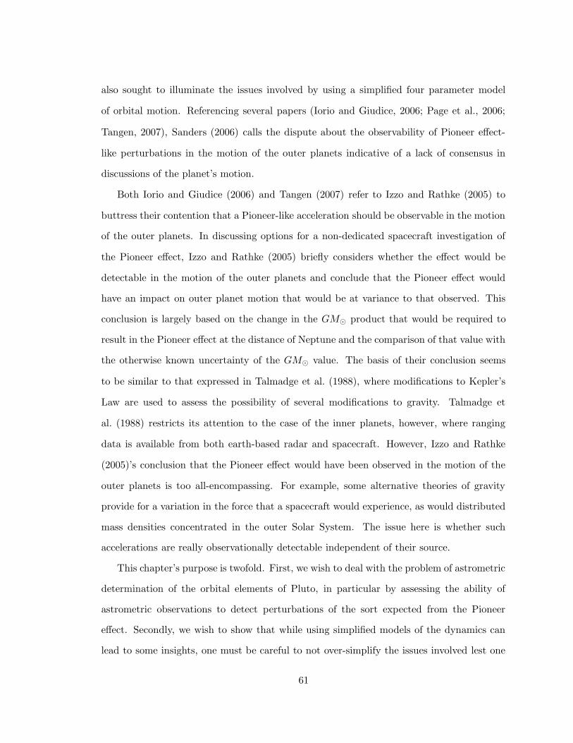
also sought to illuminate the issues involved by using a simplified four parameter model

of orbital motion. Referencing several papers (Iorio and Giudice, 2006; Page et al., 2006;

Tangen, 2007), Sanders (2006) calls the dispute about the observability of Pioneer effect-

like perturbations in the motion of the outer planets indicative of a lack of consensus in

discussions of the planet’s motion.

Both Iorio and Giudice (2006) and Tangen (2007) refer to Izzo and Rathke (2005) to

buttress their contention that a Pioneer-like acceleration should be observable in the motion

of the outer planets. In discussing options for a non-dedicated spacecraft investigation of

the Pioneer effect, Izzo and Rathke (2005) briefly considers whether the effect would be

detectable in the motion of the outer planets and conclude that the Pioneer effect would

have an impact on outer planet motion that would be at variance to that observed. This

conclusion is largely based on the change in the GM product that would be required to

result in the Pioneer effect at the distance of Neptune and the comparison of that value with

the otherwise known uncertainty of the GM value. The basis of their conclusion seems

to be similar to that expressed in Talmadge et al. (1988), where modifications to Kepler’s

Law are used to assess the possibility of several modifications to gravity. Talmadge et

al. (1988) restricts its attention to the case of the inner planets, however, where ranging

data is available from both earth-based radar and spacecraft. However, Izzo and Rathke

(2005)’s conclusion that the Pioneer effect would have been observed in the motion of the

outer planets is too all-encompassing. For example, some alternative theories of gravity

provide for a variation in the force that a spacecraft would experience, as would distributed

mass densities concentrated in the outer Solar System. The issue here is whether such

accelerations are really observationally detectable independent of their source.

This chapter’s purpose is twofold. First, we wish to deal with the problem of astrometric

determination of the orbital elements of Pluto, in particular by assessing the ability of

astrometric observations to detect perturbations of the sort expected from the Pioneer

effect. Secondly, we wish to show that while using simplified models of the dynamics can

lead to some insights, one must be careful to not over-simplify the issues involved lest one

61

be misled by the analysis onto false paths.

Specifically, this paper shows that, contrary to recent assertions in the literature, the

current ephemeris for Pluto does not preclude the existence of the Pioneer effect. We show

that the orbit of Pluto is currently not well enough characterized to make such an assertion.

Thus we address the views alluded to above that have now propagated through a number

of papers (Bekenstein (2007); Jaekel and Reynaud (2006); Khriplovich (2007); Mbelek et

al. (2007); Minguzzi (2006); Sereno and Jetzer (2006); Zaveri (2007)). We believe that the

conclusions presented in those papers are not established unambiguously and that caution

needs to be used in drawing further inferences about the dynamics of the outer Solar System.

Notwithstanding our comments about the dangers of using simplified methods, we note

that our approach itself is a simplification. The outer planets must be dynamically assessed

as a system. In order to rigorously determine whether a small perturbation like the Pioneer

effect is detectable by astrometry, we should simultaneously include the changes it produces

in the orbits of Uranus, Neptune, and Pluto. Only in this way can all the second order

perturbations to the system be taken into account. However, in order to illustrate the ideas

concerned and the weaknesses of the approaches outlined above, we restrict our attention

here to manipulating the orbit of Pluto. This approach is further discussed in Section 4.3.

The remainder of this chapter is divided into four further sections. Section 4.1 describes

several “back of the envelope” approaches to understanding the nature of the orbital changes

that a Pioneer effect would cause, and a detailed discussion of the analysis methodology we

have chosen to make our case. Section 4.2 addresses our results in terms of the relationships

between orbital parameters and observation arc length on the observability of small pertur-

bations. Finally, Section 4.3 provides a discussion of our results and Section 4.4 presents

conclusions.

62


4.1.1 Characterizing the Pioneer effect

To begin, we must describe the working definition of the Pioneer effect used in this paper.

Following Anderson et al. (1998), we take the Pioneer effect to be manifested by a radial

acceleration, directed sunward, of magnitude 8.74×10−10 m s−2. Since the primary purpose

of this paper is to investigate the dynamical consequences of the Pioneer effect, which

apparently begin at about 20 AU from the Sun, and because there are no data indicating

a more gradual onset of the Pioneer effect, we will assume that the anomalous acceleration

begins abruptly at a heliocentric distance of 20 AU.

We recognize that this is a simplistic model of the Pioneer effect. Alternative mecha-

nisms exist that cause the acceleration to vary with object mass, orbital eccentricity, radial

distance, and other parameters of the motion. As further observations are made of the

Pioneer effect, they can be used to investigate different force models to explore various

alternatives until the Pioneer effect is either ruled out or its origin is found. However, the

current status of knowledge of the Pioneer effect argues that this simple model should be

investigated first. Additionally, a perturbation beginning somewhat closer to the Sun at

a more gradual pace would be more easily seen in the motion of the planets. As shown

recently by Standish (2008), if the Pioneer effect occurred at shorter distances from the

Sun, its effect on planetary ephemerides would have already been detected. Thus, our as-

sumptions about the Pioneer effect represent the minimum plausible perturbation given

the available data. Notwithstanding our concentration on the Pioneer effect, the analysis

presented here should be valid for any small constant perturbation to gravity in the outer

Solar System.

4.1.2 Estimating Pioneer effect manifestations

There are several ways to approach assessing whether small perturbations like the Pioneer

effect can be observed in the motions of the outer planets. For clarity, however, let us

63

make clear that we are talking of perturbations to the motion of the outer planets that

are spherically symmetric and directed towards the Sun. Perturbations due to localized

mass concentrations (i.e., Planet X) are specifically excluded. However, the latter can be

instructive. Some years ago, there were allegations that the motion of the outer planets

contained anomalies that indicated the presence of a large mass concentration in the outer

Solar System. Standish (1993) showed how these presumed anomalies in Uranus’ motion

vanish when the orbital elements are adjusted while using correct values of Neptune’s mass

as determined by spacecraft. The important point here is that it is not enough to merely

compare projected positions; rather, one must adjust the orbital elements, and even other

parameters defining the problem, to best fit observational data. There are a number of

approaches to addressing this problem.

One approach was taken by Talmadge et al. (1988) in which a variation in the value of

the astronomical unit is investigated for the inner planets. Their analysis assumes a small

eccentricity and makes use of ranging data available from radar and spacecraft observations.

This shows that quite stringent constraints are placed on the nature of gravity at scales

approximating that of the inner Solar System. In particular, any Pioneer-like acceleration

at those scales would long since have been detected.

Another approach is to consider the relative magnitudes of the acceleration due to the

Sun and that due to the Pioneer effect. This is the approach taken in Page et al. (2006),

although it was not documented in that paper. Certainly the Pioneer effect should not be

expected to have a dominating impact on the motion of the outer planets. The ratio of

the Pioneer acceleration to that produced by the Sun at a distance equal to the semimajor

axis of the outer planets is 0.005, 0.013, and 0.023 percent for Uranus, Neptune, and Pluto,

respectively. If we integrate an orbit without any perturbations to Newtonian gravity other

than the Pioneer effect, and compare with the Keplerian case, we find the orbital periods of

these objects are systematically shorter. Uranus’ period shortens by 5.8 days and Neptune’s

by 24.1 days, while Pluto’s period drops by 79.7 days. These intervals correspond to 0.02,

0.04, and 0.09 percent of the periods of Uranus, Neptune, and Pluto, respectively.

64

Differentiating Kepler’s Third Law implicitly, we obtain a relationship between a small

change in an orbiting object’s period and a corresponding change in the orbit’s semimajor

axis. In particular, da/a = (2/3)dT/T where a is the semimajor axis (in AU) and T is the

orbital period (in years). For Uranus, the fractional period shortening due to the Pioneer

effect is equivalent to a fractional change in semimajor axis of approximately 0.013 percent.

Similarly, the orbital period shortening is equivalent to a reduction in semimajor axis of

0.027 and 0.059 percent for Neptune and Pluto, respectively.

These simple calculations imply an equivalent change in aphelion distance of 3.8 × 105,

1.2 × 106, and 4.3 × 106 km for Uranus, Neptune, and Pluto. In the cases of Uranus and

Neptune, this is less than the approximate maximum errors in range of 2× 106 km (Seidel-

mann, 1992)). In the case of Pluto, the change in semimajor axis that would correspond to

the shortening of its orbital period with the Pioneer effect is about twice the radial distance

uncertainty. However, Pluto has completed less than one-third of an orbit since its discovery

and its orbital elements are even less well-determined than the other outer planets. Thus,

small changes in other orbital elements could easily obscure any orbital changes due to the

Pioneer effect.

4.1.3 Celestial mechanics

The values of orbital elements are not directly observable and to reduce observational data

to orbital elements it is necessary to proceed by using numerical approximations.2 The

normal manner in which one proceeds is to first determine a “preliminary orbit” from a

small number of observations and then to refine it by successive approximations into a

“definitive orbit” as many more observations are added.

The method used to improve the orbit and obtain the definitive orbit through additional

observations is called “differential correction” and is well described in standard celestial

2 In this discussion we are dealing with “classical” observations consisting of two angles describing theposition of the object in the sky at a moment in time. Orbital determination when one has range information,for example with radar observations, is a completely different mathematical problem. This latter areais sometimes called “astrodynamics.” Radar observations for objects subject to the Pioneer effect are

technologically out of the question for the foreseeable future.

65

mechanics texts (e.g., Moulton (1914), Brouwer and Clemence (1961), or Danby (1988)).

Differential correction uses a least squares approach to iteratively refine the estimates of

the elements as more observations become available. Additionally, statistical information

on the errors of the elements naturally results from the differential correction process. The

process results in a set of orbital elements, along with error estimates for the elements and

covariance parameters showing the degree to which the elements are correlated. It is worth

remembering that the equations governing celestial mechanics are nonlinear and normally

a linearized version of the problem is used to determine the covariances and elements.

However, the nonlinearity manifests itself in occasional difficulties in determining elements

and some of these difficulties will be discussed later in Section 4.2.2.

The whole chain of analysis outlined above for orbital element determination is as-

sociated with a number of errors that must be understood and characterized. Some are

associated with the description of the Solar System dynamics and calculation of the orbits,

while some originate in the observations themselves.

However, in determining elements from observations, there is no prior warning about

the pathological situations that can arise. For example, if the inclination is small, the error

in the longitude of the ascending node will be large. Similarly, if the eccentricity is small,

the error in the argument of perihelion will be large and the time of perihelion passage or

mean anomaly will be poorly defined. Such problems can be avoided through the use of

alternative orbital elements (e.g., equinoctial elements).

Thus, the orbital characterization process outlined above must be carried out to enable

predictions of the future positions of objects on the sky. The errors associated with the pre-

dictions must be compared statistically to determine whether a truly observable difference

can be asserted between the alternative models of gravity.

Importantly, since orbital elements are not directly observable, it is not enough to simply

integrate an object’s equations of motion forward in time from a set of initial conditions,

with and without the perturbation (as was done in Iorio and Giudice (2006)), and then

compare the differences. One must first determine element values by adjusting them to a

66

set of observations and a gravity model to obtain a new set of elements with associated error

metrics. This can be understood physically by noting that the orbital elements describe

the conserved mechanical energy of the body and if the potential field changes due to the

existence or absence of a perturbation the elements need to be redetermined.

In order to address these issues, we use the OrbFit software package (Milani, 1999). This

program uses observational data and data on the dynamics of the Solar System to determine

orbital elements and predict ephemerides for minor bodies. Since OrbFit is available in

source code, we added a simple option to include forces arising from the Pioneer effect. By

comparing orbits resulting from synthetic observations with and without the Pioneer effect,

we explore the expected effects of such a perturbation on asteroid orbits and examine when

this effect can be detected astrometrically.

OrbFit is a complex piece of software that performs a number of tasks that relate to

this analysis. The first task of interest here is that of orbit determination. This process

begins with astrometric observations of the body of interest. An initial orbit is determined

from a few of the available observations and a process of differential correction is applied

to correct the initial elements and take into account any additional observations.

The second task of interest performed by OrbFit is orbital position prediction. To

predict the position of bodies of interest, OrbFit takes the position and velocity of the

body of interest, and integrates the equations of motion of that body with many additional

perturbations due to the other bodies in the Solar System, Solar oblateness, etc.

Additionally, the process used by OrbFit naturally provides measures of the errors in

elements that result from the unavoidable errors in position measurement and the associated

element covariances. These data can be mapped on to positions in the sky and the error

associated with the prediction, which permit our analysis to take place.

By using OrbFit for our calculations, we are able to include planetary and other per-

turbations and factors that affect the determination and prediction of orbits. These factors

are dealt with in OrbFit to create orbital predictions and also conduct orbital analyses in a

manner that very closely mimics the process by which data from observations are reduced

67

to orbital predictions and elements in the real world. In particular, OrbFit is able to deal

with various errors and noise that are both unavoidable and necessary for calculations at a

level of accuracy sufficient for distinguishing between orbits affected by the Pioneer effect

and those subject to gravity without the additional perturbation.

The calculations outlined above represent standard techniques of celestial mechanics and

can be performed by any number of systems. OrbFit was chosen because of its availability

in source code. This permitted addition of a simple option to include the force arising from

the Pioneer effect, which were simply added to the forces exerted on the bodies of interest

by the major planets.

Rather than integrating the orbits of the main bodies in the Solar System, their dynamics

are introduced via the JPL DE405 ephemeris. In this context the planetary ephemeris is a

sort of lookup table containing positions of the planets so that their effect on the motion of

a body of interest might be determined.

4.1.4 Simulation of observations

In this paper, we will parametrically vary the eccentricity of hypothetical test bodies, gen-

erate synthetic observations for them with– and without a Pioneer-like acceleration, and

determine the conditions under which the Pioneer effect can be observed. With the excep-

tion of eccentricity, the orbital elements of our test bodies are those of Pluto (Seidelmann,

1992). The eccentricity of the bodies are 0.001, 0.005, 0.01, 0.05, 0.1, 0.2, and 0.3. These

values are chosen to bracket the actual eccentricity of Pluto while extending to nearly cir-

cular orbits similar to those found in the other outer planets. The nominal elements at the

epoch J2000 (JD 2,451,545.0), are referred to the mean ecliptic and equinox of JD 2000.0

and are given in Table 4.1.

The observation cadence we have chosen to use roughly reflects that which exists for

Pluto. If one reviews the observations for Pluto that were used to construct the DE405

ephemeris, we find approximate observation frequencies as indicated in Table 4.2. With

68

Table 4.1 Elements for the hypothetical bodies used in the analysis.

Element Valuea

Semimajor axis 39.48168677 AUEccentricity See textInclination 17.14175 degreesLongitude of Ascending Node 110.30347 degreesArgument of Pericenterb 113.76329 degreesMean anomalyc 14.86205 degrees

a Source for element values is Seidelmann (1992)b The argument of the pericenter is equal to the differencebetween the longitude of pericenter and the longitude of theascending node.c The mean anomaly is the mean longitude minus the lon-gitude of pericenter.

the exception of the 1914-1929 period, we have adopted these cadences and generate syn-

thetic observations accordingly. The pre-discovery observations occuring from 1914-1929

are aggregated and an overall rate of one observation per year is used for this time period.

In the analysis, we use observation arc lengths running up to 250 years that are eval-

uated at 50 year intervals. Since the orbital period of these objects is approximately 250

years, our synthetic observations span a complete orbit. The total number of synthetic ob-

servations occurring over the observation arc lengths are shown in Table 4.3. The number

of observations and their frequency is approximately that actually existing for Pluto, with

reasonable extrapolations into the future.

The general approach is to use OrbFit with a set of elements defined as described

in Table 4.1 to generate ephemerides separately in both the perturbed (that is, with the

Pioneer perturbation present), and unperturbed (without the Pioneer effect) cases. The

predicted positions of the test body on the sky represent “perfect” observations with no

uncertainties in either observations or elements. In each case, we can take these predicted

ephemeris positions and add Gaussian observational error. These randomly altered positions

then represent the results of synthetic astrometric observations. The random observational

error applied is equal to 0.3 seconds of arc, representing the results of good quality CCD

69

Table 4.2 Frequency of archive observations of Pluto.

Dates No. Observations No. Years Approx. Cadence

1914-1919 11 6 2 per year1920-1929 6 10 1 per 2 years1930-1939 431 10 1 per week1940-1949 233 10 2 per month1950-1959 113 10 1 per month1960-1969 113 10 1 per month1970-1979 364 10 3 per month1980-1989 361 10 3 per month1990-1999 1,125 10 1 per 3 days2000-2006 962 7 1 per 3 days2007-2011 est. 5 1 per 3 daysa

2012-2163 est. 152 1 per dayb

a Continue 2000-2006 cadence.b Continue 2000-2006 cadence, but assume that LSST and Pan-STARRScome online in 2012 and each produces one observation every three daysfor a total observation cadence of one observation per day.

astrometry reduced against modern star catalogs. This value of error is assumed to be

isotropic on the sky; thus, we generate and apply synthetic errors in right ascension and

declination equal to this value divided by the square root of two with appropriate adjustment

to the Right Ascension for the cosine of the declination. The resulting different sets of

synthetic observations and alternative gravity models can then be used with OrbFit to

determine elements and errors associated with the elements as a function of the eccentricity

and the observation arc length. It is noted that this is the procedure used to investigate

the motion of minor planets in Page et al. (2006) and Wallin et al. (2007).

We recognize that this assumed error represents a level of accuracy much better than

that found in observations taken until relatively recently. Indeed, there are many potential

sources of position error that might be modeled, some of a known nature and some unknown.

The data were taken at different observatories and different techniques may have been used

to reduce the observations, leading to systematic errors in the derived positions. The

positions have been reduced with various catalogs and transformed, sometimes repeatedly,

70

Table 4.3 Total number of synthetic observations used in analysis, for each arc segmentevaluated.

Arc Segments No. Observations Cum. Observations

1914-1963 952 9521964-2013 4,212 5,1642014-2063 18,262 23,4262064-2113 18,262 41,6882114-2163 18,262 59,950

to different reference frames. Even for modern observations, there may be errors in the

adopted precession values for the J2000 epoch. Additional error sources include errors due

to uncertainties of the initial conditions of the other planets (e.g., ephemeris errors), errors

due to corrections to earth rotation, and unmodeled instrumental corrections.

Since the primary impact of increasing the a priori positional error is to de-emphasize

those observations with larger errors, we chose to equally weight all our synthetic observa-

tions. Thus, we assume much more optimistic error estimates for early observations than

are representative in the actual observation archive and results in equal weighting for all

the synthetic observations. This should result in our calculations providing an optimistic

estimate of the detectability of the Pioneer perturbation.

An additional reason for electing to model a uniform observational accuracy across the

span of the synthetic observations in order to minimize variation in our results due to

another source of observational noise. For parts of the synthetic observational arc prior

to the advent of modern catalogs and CCDs, this error will be considerably less than that

found in the actual observational archive. Interestingly, the OrbFit program is capable of

varying a priori observational error across time or across different observatories, but we did

not make use of this capability in this paper.

Given these assumptions, we have four cases, which we illustrate in Table 4.4. The first

pair of cases (the “Gravity with PE” column in Table 4.4), and the focus of our analysis,

is for observations that are generated with a Pioneer-effect perturbation present meaning

71

Table 4.4 Four cases combining gravity models and forces determining motion.

Forces Determining Motiona

Gravity Modelb Gravity with PEc Only Gravityd

Gravity with PEc “Matched” “Mismatched”Only Gravityd “Mismatched” “Matched”

a By this we mean that the motion of the orbiting objects are deter-mined by the forces indicated. The first column indicates that thereis really a Pioneer effect perturbation superimposed on Newtoniangravity; the second column indicates that there is not an additionalperturbation.b “Gravity Model” refers to the assumed force law to which theorbital observations are fit. The first row corresponds to the casewhere the assumed force law is Newtonian gravity with an additionalPioneer-like constant acceleration; the second row refers to a forcelaw purely Newtonian in character.c “Gravity with PE” indicates that there is a Pioneer effect pertur-bation.d “Only gravity” indicates that there is no Pioneer effect perturba-tion.

that the Pioneer effect exists in Nature and determines an object’s motion. These same

observations are analyzed with two gravity models. The first model is that of Newtonian

gravity with the addition of a constant radial acceleration with a value commensurate with

that associated with the Pioneer effect; the second is standard Newtonian gravity. The

comparison of the orbital solutions for these two cases correspond to a situation in which

the universe is one where the Pioneer effect actually exists and we analyze it to determine

which of our two gravity models is correct. This is the situation portrayed in the first column

of Table 4.4. The second pair of cases are comparable except that they are associated with a

universe where the Pioneer effect does not exist. Again, we compare two theories of gravity

to see if we can observationally distinguish between the two. This situation is portrayed

in the second column of Table 4.4. This paper investigates the first case only; as shown in

Page et al. (2006), the second case is nearly symmetric with the first, and produces similar

conclusions.

72

4.2 Results

4.2.1 Prediction of sky position from orbital elements

Projected orbits

As outlined above, our plan is to take ephemerides created with various known orbital

elements and predict positions on the sky when the motion is governed by Newtonian

gravity with– and without a Pioneer-like perturbing acceleration. This process involves

integrating the equations of motion of a body subjected to two different force laws.

The results of this calculation provide sky positions as a function of time. Since the

angular differences between the predicted positions are small, we separately consider the

difference in right ascension and declination resulting from the two situations. Fig. 4.1

shows the resulting position difference. The orbits have elements given in Table 4.1, except

for the eccentricity which is parametrically varied. Since the epoch of the elements is JD

2,451,545.0, the angular differences are zero at that date and diverge as one moves forward

and backwards in time from the element epoch. It is worth emphasizing that the two

ephemerides being compared are generated with two separate gravity models with identical

and exactly specified elements.

Figure 4.1 can be compared with Figs. 9 and 10 in Iorio and Giudice (2006). They drew

the conclusion that the divergence in position, since not observed over the past 90 years,

indicates the Pioneer effect does not exist. However, such a conclusion is based on the

idea that the elements (i.e., the initial conditions) are known precisely. The reality is that

these position predictions are those related to the elements derived from the assumption of

Newtonian gravity coupled with observed positions. If there is a “mismatch” between the

gravity model used to derive orbital elements and the reality that determines the actual

motion of the orbital bodies, these will not be the correct elements. Even if the elements are

derived from a “matching” reality and gravity model, it is remarkable how rapidly orbital

predictions can degrade outside the observation arc, especially when that arc is short relative

to the orbital period. These aspects will be discussed in detail in the next subsection.

73

-200

-100

0

100

200

300

400

500

600

1900 1950 2000 2050 2100 2150 2200

(WP

E -

WO

PE

) R

ight

Asc

ensi

on D

iffer

ence

(ar

csec

)

Time (year)

Panel A

e = 0.001e = 0.005e = 0.010e = 0.050e = 0.100e = 0.200e = 0.300

-40

-20

0

20

40

60

80

100

120

140

1900 1950 2000 2050 2100 2150 2200

(WP

E -

WO

PE

) D

eclin

atio

n D

iffer

ence

(ar

csec

)

Time (year)

Panel B

e = 0.001e = 0.005e = 0.010e = 0.050e = 0.100e = 0.200e = 0.300

Figure 4.1 Angular position differences when orbits are extrapolated with “known” elementswith– and without a Pioneer effect perturbation. Panel A (left) shows the right ascensiondifference between the perturbed and unperturbed cases. Panel B (right) similarly showsthe declination difference.

74

Fitted orbits

If we take the ephemeris positions associated with one “reality” (e.g., the one containing

the Pioneer perturbation—see Table 4.4) consonant with the observation cadence shown

in Table 4.2, and add an isotropic, normally distributed random position error of 0.3 arc

seconds to each of the positions, the result is a set of synthetic positions that are illustrative

and representative of those that might have been obtained as observations of the bodies.

This set of observations can be divided into five different arcs covering 250 years (approx-

imately one orbital period); thus, each arc covers an additional 50 years from the start of

the observations and represents an incremental one-fifth of an orbital revolution.

Each synthetic observation arc can be analyzed when a Pioneer-like perturbation is

included and when it is not, corresponding to the two rows in the first column of Table 4.4.

The observation fitting process serves to determine the elements of the orbit and these are

the elements that can then be used to predict sky position. How do the observed positions

differ when this procedure is followed?

Figs. 4.2 through 4.6 shows the difference in sky position as a function of time for the

orbital fits associated with the two gravity models. The elements are those given in Table 4.1

except for eccentricity which is varied parametrically. In all cases, the left hand graph shows

the right ascension difference while the right hand graph shows the declination difference.

Comparing these figures with Fig. 4.1 above and Figs. 9 and 10 in Iorio and Giudice (2006)

shows that for shorter arcs (those ranging up to 100 years long) the difference in predicted

motion for the two gravity models is quite small for the duration of the observation arc

and only begins to substantially diverge when the position is being extrapolated to times

beyond those for which observations exist. For a 150 year arc, small irregularities in the

position difference begin to be noticeable during the observational arc. As the arcs grow

still longer (to 200 years and beyond), more substantial irregularities are seen. Also, it is

generally true that positional differences are greater the greater the eccentricity, all other

things being equal.

75

-50

0

50

100

150

200

250

1900 1950 2000 2050 2100 2150 2200

(WP

E -

WO

PE

) R

ight

Asc

ensi

on D

iffer

ence

(ar

csec

)

Time (year)

Arc: 1914-1963

Panel A

e = 0.001e = 0.005e = 0.010e = 0.050e = 0.100e = 0.200e = 0.300

-20

0

20

40

60

80

1900 1950 2000 2050 2100 2150 2200

(WP

E -

WO

PE

) D

eclin

atio

n D

iffer

ence

(ar

csec

)

Time (year)

Arc: 1914-1963

Panel B

e = 0.001e = 0.005e = 0.010e = 0.050e = 0.100e = 0.200e = 0.300

Figure 4.2 Angular position difference when orbits are extrapolated with elements deter-mined from synthetic observations generated with a Pioneer effect perturbation over a 50year arc. Panel A shows the difference in right ascension between determining the orbitalposition with a gravity model including the perturbation and one not including the Pioneereffect. Panel B shows the similar declination difference.

76

-50

0

50

100

150

200

250

1900 1950 2000 2050 2100 2150 2200

(WP

E -

WO

PE

) R

ight

Asc

ensi

on D

iffer

ence

(ar

csec

)

Time (year)

Arc: 1914-2013

Panel A

e = 0.001e = 0.005e = 0.010e = 0.050e = 0.100e = 0.200e = 0.300

-20

0

20

40

60

80

1900 1950 2000 2050 2100 2150 2200

(WP

E -

WO

PE

) D

eclin

atio

n D

iffer

ence

(ar

csec

)

Time (year)

Arc: 1914-2013

Panel B

e = 0.001e = 0.005e = 0.010e = 0.050e = 0.100e = 0.200e = 0.300


77

-50

0

50

100

150

200

250

1900 1950 2000 2050 2100 2150 2200

(WP

E -

WO

PE

) R

ight

Asc

ensi

on D

iffer

ence

(ar

csec

)

Time (year)

Arc: 1914-2063

Panel A

e = 0.001e = 0.005e = 0.010e = 0.050e = 0.100e = 0.200e = 0.300

-20

0

20

40

60

80

1900 1950 2000 2050 2100 2150 2200

(WP

E -

WO

PE

) D

eclin

atio

n D

iffer

ence

(ar

csec

)

Time (year)

Arc: 1914-2063

Panel B

e = 0.001e = 0.005e = 0.010e = 0.050e = 0.100e = 0.200e = 0.300


78

-50

0

50

100

150

200

250

1900 1950 2000 2050 2100 2150 2200

(WP

E -

WO

PE

) R

ight

Asc

ensi

on D

iffer

ence

(ar

csec

)

Time (year)

Arc: 1914-2113

Panel A

e = 0.001e = 0.005e = 0.010e = 0.050e = 0.100e = 0.200e = 0.300

-20

0

20

40

60

80

1900 1950 2000 2050 2100 2150 2200

(WP

E -

WO

PE

) D

eclin

atio

n D

iffer

ence

(ar

csec

)

Time (year)

Arc: 1914-2113

Panel B

e = 0.001e = 0.005e = 0.010e = 0.050e = 0.100e = 0.200e = 0.300


79

-50

0

50

100

150

200

250

1900 1950 2000 2050 2100 2150 2200

(WP

E -

WO

PE

) R

ight

Asc

ensi

on D

iffer

ence

(ar

csec

)

Time (year)

Arc: 1914-2163

Panel A

e = 0.001e = 0.005e = 0.010e = 0.050e = 0.100e = 0.200e = 0.300

-20

0

20

40

60

80

1900 1950 2000 2050 2100 2150 2200

(WP

E -

WO

PE

) D

eclin

atio

n D

iffer

ence

(ar

csec

)

Time (year)

Arc: 1914-2163

Panel B

e = 0.001e = 0.005e = 0.010e = 0.050e = 0.100e = 0.200e = 0.300


80

Recall what the differences plotted in Figs. 4.2 through 4.6 represent. Synthetic ob-

servations for a universe with a Pioneer effect were generated and orbital elements were

determined by fitting the same observations to two alternative gravity models. One of

these models is correctly “matched” to the observations; that is, the gravity model used for

orbit fitting is the same one used to generate the observations. The other model does not

correspond to the one used to generate the observations. Thus, we would a priori expect

that the former would fit the data better than the latter.

What we see, however, is surprising. For observation arcs as long as a century, which at

best is the situation obtaining for Pluto at the current time, there are only relatively small

differences in the positions predicted by the correct gravity model and those predicted by

the mismatched model. In all cases, however, the predicted positions outside the range of

observations rapidly diverge from one another.

This behavior is a manifestation of two inter-related factors. First, the orbital fitting

problem is inherently nonlinear and is normally solved in the linear approximation. Even

if not mathematically chaotic, the system of equations is certainly sensitively dependent

upon initial conditions; small changes in elements can result in large changes in predicted

position outside the range of observations. Secondly, this sensitivity is exacerbated by the

problem of a short observation arc. The length of the entire observational archive for Pluto

is no more than about one-third of its orbital period. Even in as simple a case as linear

least squares curve fitting, a limited amount of independent variable data (corresponding

to a short observation arc) will lead to relatively large errors in the fitting parameters

(corresponding to the orbital elements). Together, these factors conspire to potentially

generate large position errors outside the observation arc, while increasing the length of the

observation arc can markedly reduce error over the whole of the arc and even beyond it.

Some of these issues can sometimes be alleviated by a change in variables. Use of other

than Keplerian orbital elements (e.g., equinoctial elements) can allow one to avoid some

problems with determining an orbital solution, in particular in cases with small eccentricities

or small inclinations. Similarly, a linear combination of Keplerian orbital elements can be

81

used to improve the accuracy of some elements (but see the footnotes on pages 92 and

93). However, those types of variable change do nothing for the issues associated with the

ill-conditioned nature of the linear matrix and a short observational arc.

In any case we see that we must fit observations to particular gravity models and adjust

orbital elements before predicted positions on the sky can be compared. Noting that deriving

orbital elements and predicting an orbit beyond a short observation arc provides little

information about the actual motion that will be seen once new observations are made, we

conclude that drawing conclusions from such extrapolations is totally unwarranted. Thus,

we can conclude nothing regarding the Pioneer effect and the motion of Pluto as it is

currently known, at least subject to the limitations of our methodology.

Now let us examine more closely the relatively small position differences at the beginning

of the observation arcs in Figs. 4.2 through 4.6. Fig. 4.7 is similar to Figs. 4.2 through

4.6, but shows an expanded view of the difference in position of a body with an eccentricity

of 0.3 (e.g., similar to Pluto) and a 100 year observation arc. At the beginning of the arc,

the difference in right ascension for the two gravity models is nearly six seconds of arc and

the difference in declination is about 1.5 arcsec. One would certainly think that this level

of difference would be observable; however, we argue below that it is not a distinguishable

difference given our current knowledge of Pluto’s orbit.

Figure 4.8 shows a subset of the residuals in both right ascension and declination of

actual observations with respect to a recent JPL ephemeris, DE414. The full set of residuals

show a number of clear outliers and we have removed from the set any residuals of magnitude

greater than ten seconds of arc. Prior to about 1960 there is clearly a greater spread in

the residuals than at later times. Additionally, prediscovery images taken prior to 1930

and dating to as early as 1914 have been found in the archive. These observations seem

to contain serious irregularities manifested by large and systematically biased residuals.

Supporting this assertion, Gemmo and Barbieri (1994) find that systematic differences

between the observed and calculated orbit are a continuing issue. Additionally, they find

that only about half of Pluto’s motion since its discovery has been observed in a systematic

82

-10

-5

0

5

10

0.00 0.05 0.10 0.15 0.20 0.25 0.30 0.35 0.40

(WP

E -

WO

PE

) R

ight

Asc

ensi

on D

iffer

ence

(ar

csec

)

Fraction of an Orbital Revolution

Panel A

-10

-5

0

5

10

0.00 0.05 0.10 0.15 0.20 0.25 0.30 0.35 0.40

(WP

E -

WO

PE

) D

eclin

atio

n D

iffer

ence

(ar

csec

)

Fraction of an Orbital Revolution

Panel B

Figure 4.7 Angular position differences for Pluto when orbits are predicted with elementsdetermined from synthetic observations generated with a Pioneer effect perturbation. Thetime axis is labeled in units of Pluto’s orbital period running from the beginning of modernobservations up to the present. Panel A shows the difference in right ascension betweendetermining the orbital position with a gravity model including the perturbation and onenot including the Pioneer effect. Panel B shows the similar declination difference.

83

and organized manner. They also comment that it is impossible to extrapolate Pluto’s

position more than a few years into the future. This is indicative of a poorly characterized

orbit.

The residuals of the synthetic observations with respect to a “mismatched” gravity

model are similar in character and magnitude to the differences between predictions for

different gravity models that are shown in Fig. 4.7. As observed previously, there seems to

be a significant difference between the two sets of predictions. A standard comparison of

these models (Bevington and Robinson, 2003) would calculate and compare χ2 values for

the two models. If the resulting value is about unity, the fit is good.

The overall issues associated with model goodness-of-fit are complex and will be dis-

cussed later in Section 4.2.3; however, anticipating this complexity let us look more deeply

at the data. If we compare our “mismatched” orbit fit with actual observational data and

their associated fit, we will see that there are comparable systematic errors in both the

synthetic and the real datasets.

Simulated post-fit residuals with respect to the DE414 ephemeris

Systematic trends in residuals can be visually discerned more readily by examination of

normal points rather than individual data points. In a normal point plot, means and

standard deviations of the residuals are collected and plotted for each planetary opposition.

Fig. 4.9 shows the normal points for the DE414 residuals in the “high-low-close” portion

of the plot, where the “closing” value indicated by the small horizontal mark is the average

residual for each opposition and the length of the vertical line indicates a one standard

deviation variation above and below the mean residuals. The comments above about the

systematic bias of the prediscovery observations and the larger dispersion of residuals before

1960 are borne out in the normal plot.

Now, let us compare this data with normal points for the synthetic observations of

Pluto. In developing the observation cadence for the synthetic observations, we did not

consider the relative positions of the Earth, the Sun, and Pluto and thus did not concentrate

84

-10

-5

0

5

10

1900 1920 1940 1960 1980 2000 2020

Res

idua

ls (

arcs

ec)

Year

Panel A

-10

-5

0

5

10

1900 1920 1940 1960 1980 2000 2020

Res

idua

ls (

arcs

ec)

Year

Panel B

Figure 4.8 Observed minus calculated residuals for Pluto with respect to the DE414ephemeris. Panel A provides the right ascension residuals in arc seconds while Panel Bgives the declination residuals. The same scale is used in this figure as in Fig. 4.7.

85

-6

-4

-2

0

2

4

6

1900 1920 1940 1960 1980 2000 2020

Res

idua

ls (

arcs

ec)

Year

Panel A

-6

-4

-2

0

2

4

6

1900 1920 1940 1960 1980 2000 2020

Res

idua

ls (

arcs

ec)

Year

Panel B

Figure 4.9 Normal points for the DE414 residuals and the residuals for the synthetic obser-vations relative to their ephemeris. Panel A pertains to the right ascension residuals whilePanel B applies to the declination residuals.

86

synthetic observations around particular yearly oppositions. Since our primary purpose was

to illustrate broader issues with the data, this was done to avoid introducing additional noise

through a varying observational cadence. Thus, for the post-discovery residuals associated

with our synthetic observations we found the average and standard deviations for each

calendar year. For prediscovery images, our assumed observation cadence of one observation

per year clearly made the dispersion calculation impossible. In these cases, we accumulated

data by decade; thus, we calculated the mean and standard deviation for the 1914-1919

period and the 1920-1929 period and plotted the resulting values accordingly.

The normal points associated with the synthetic observations are also shown in Fig.

4.9. The average is shown by the solid line and the plus and minus one standard deviation

limits are shown as dotted lines. Several comments are in order about these graphs. First,

the width of the standard deviation spread on the synthetic observations is different from

that of the DE414 residuals. This is due to our assumption of a constant 0.3 arc second

astrometric accuracy of the synthetic observations. The actual observations that contribute

to the dispersion of the DE414 residuals have varying accuracies, ranging from large values

for the early observations to small values for current CCD observations. As pointed out

earlier, the level of astrometric accuracy used in the synthetic observations is much better

than that found in the actual observation archive until relatively recently. We chose to

model a uniform observational accuracy across the span of our synthetic observation arc in

order to make an optimistic estimate of the detectability of the Pioneer perturbation as well

as to minimize variation in our results due to another source of noise (e.g., the observation

error). Thus, rather than the uniform difference between the upper and lower limits, the

normal points of the actual DE414 residuals vary in width. If we had modeled a varying

error, such a variation in width would be expected for the synthetic observations as well.

Another point to be made about Fig. 4.9 is that while the prediscovery residuals for

the synthetic observations and those with respect to DE414 are of opposite signs, their

magnitudes are of the same order. In the former case, the large residuals are due to fit-

ting a “mismatched” gravity model consisting of only nominal gravity to observations that

87

result from gravity plus an anomalous Pioneer acceleration; in the latter case, unknown

observational errors have resulted in large and biased residuals. What are we to make of

the difference in sign? We would argue that since there are errors of an unknown nature

present in these early observations, we have absolutely no basis is even assuming the sign of

the residual is indicative of reality. Although the prediscovery residuals have characteristics

that indicate that they might represent a constant offset in right ascension, an effect that

can be caused by many errors in the analysis of the observations, the limits on the resid-

ual’s variation can also accomodate a linear trend as is seen in the corresponding synthetic

observations. We can only observe that the approximate magnitude of the residuals at

early times are roughly the same for both real observations relative to the DE414 ephemeris

and the synthetic observations with respect to their ephemeris. Thus, we cannot draw

any conclusions about the existence or nonexistence of the Pioneer effect from our current

knowledge of the orbit of Pluto; its observation arc is too short for such a determination.

A third point with respect to Fig. 4.9 is that post-discovery residuals are similar for both

the synthetic observations and those of DE414 and very close for post-1960 observations.

Overall, the only place where the two sets of normal points diverge is in the prediscovery

era. Thus, neither set seems to indicate the existence or nonexistence of an additional

gravitational anomaly. Both sets of residuals possess patterned irregularities, but it is

impossible to say that one is superior to the other.

As a final comment on the comparison of the two sets of residuals, Fig. 4.10 shows

the total rms residual by epoch for the two cases. This quantity is the square root of the

sum of the squares of the residuals in right ascension and declination with an appropriate

adjustment for the cosine of the declination. As above, DE414’s residuals are accumulated

by opposition, while the residuals of the synthetic observations relative to their ephemeris

are accumulated by decade for prediscovery observations and by year thereafter. The quality

of the residuals in the two cases is quite high over most of the observation arc. Even in the

prediscovery era, the trends of the residuals are similar. As before, there is a linear trend

in the synthetic residuals, but the entire prediscovery regime only includes two points. The

88

0

1

2

3

4

5

6

1900 1920 1940 1960 1980 2000 2020

rms

Res

idua

ls (

arcs

ec)

Year

Figure 4.10 Total rms residual by epoch for the DE414 case and the synthetic observationcase. The points show DE414’s rms residual accumulated by opposition. The lines showthe rms residual of the synthetic observations relative to their ephemeris accumulated bydecade for prediscovery observations and by year thereafter.

trend of those two points is not dissimilar to that of the DE414 residuals. Even if the

prediscovery observations possessed a systematic error of as large as two seconds of arc, the

trend in rms residual is not substantially different from those of the synthetic observations.

From the discovery of Pluto to about 1960, the DE414 total rms residuals are greater

than those found for the synthetic observations. This difference is expected due to the

conservative assumptions of astrometric accuracy that were made in generating the synthetic

observations. However, the trend of the residuals in both cases is similar, indicating a

comparable fit to the observations. From about 1960 to the mid-1990s, both sets of residuals

fit quite well. From about the mid-90s on, the actual residuals are somewhat less that those

associated with our synthetic observations. This would represent the first sign that the

orbit of Pluto fits one gravity better than another.

Given the likely, but uncharacterized, errors in pre-discovery observations, we are led to

the observation that real observations are explained about as well by DE414 as the synthetic

89

observations are explained by their ephemeris.

The context of this comment must be kept in mind. The DE414 residuals relative to its

ephemeris represent a fit to the actual observation archive by a normal gravity model without

a Pioneer anomaly. The synthetic observations are created with a Pioneer anomaly present

and thus their underlying motion is not in keeping with normal gravity. When the synthetic

observations are fit to a gravity model without a Pioneer anomaly included in the dynamics,

the fit is almost indistinguishable from that of the DE414 ephemeris. Especially given the

uncharacterized errors apparently present in the prediscovery observation archive, we cannot

distinguish between the two gravity models on the basis of the current observational record.

However, we note that this is at least as much due to the shortness of the observation arc

for Pluto as due to any difference in gravity models.

What adds special interest to the Pluto case, however, is that due to its relatively large

eccentricity Pluto shows potentially detectable differences between the two gravity models if

the entire one hundred year observation arc were uniformly reliable. Thus, we are led again

to the desirability of continuing to gather astrometric data on Pluto and expect that an

astrometric difference in position might soon be able to falsify the existence of the Pioneer

anomaly. Nevertheless, for the length of the currently available observation arc and because

of the uneven quality of the observational archive, we cannot currently distinguish between

the two gravity models on the basis of orbital position.

4.2.2 Errors in orbital elements derived from observations

There are six orbital elements corresponding to the six degrees of freedom of the classical

dynamical problem in three dimensions. Given that elements are determined from obser-

vations by a model fitting process, we must ask whether this large number of degrees of

freedom is somehow redundant and whether a simpler model of the dynamics can be used

to illuminate the problem.

This is the approach taken by Tangen (2007), where synthetic observations are generated

for a simplified dynamical model with four degrees of freedom. Conclusions are then drawn

90

about the degree to which a Pioneer effect perturbation can be fit to this simplified model

and thus whether the Pioneer effect exists.

The problem with this approach is that the elements that are ignored or suppressed in

Tangen (2007) are precisely those with the greatest uncertainty resulting from the orbital

fitting process. Further, as will be discussed below, care must be taken when using rms

residuals as a primary measure of goodness of fit as far as model selection is concerned.

The underlying cause of the problems outlined above was discussed earlier. Briefly, this

behavior is due to two inter-related factors: First, the orbital fitting problem is inherently

nonlinear and is normally solved in the linear approximation; second, the sensitivity of

the orbital solution to initial conditions is exacerbated, especially in the case of Pluto, by

the problem of a short observation arc. These issues can sometimes be alleviated by a

change in variables. Use of other than Keplerian orbital elements can result in an improved

determination of orbital elements (Brouwer and Clemence, 1961). However, this type of

variable change does nothing for the issues associated with a short observational arc. The

uncertainties arising from these sources make the approach in Tangen (2007) problematic.

In simplifying the problem by assuming away two or more degrees of freedom, the full

parameter space, which has ample room to conceal the differences in predicted position, is

not available for that purpose. This provides the false impression that perturbation effects

are observable when, in fact, they are not.

One might think that the Pioneer acceleration, assumed to be radial, would only effect

the motion of an orbiting body in its orbital plane. In a theoretical sense, this is true.

The Pioneer effect exerts no torque on the orbiting body, and the plane of the orbit re-

mains unchanged as time progresses. An analytical investigation of such an orbit can be

considered as two dimensional and the number of degrees of freedom of the motion can be

reduced accordingly. This is the essence of the approach of Tangen (2007). However, in an

observational context the motion is not restricted to a plane. There are at least two factors

that force orbital motion to be considered to occur in three dimensional space with the

associated degrees of freedom. The first is that unless the observer’s location (e.g., Earth)

91

remains in the plane of the orbit of the body, there will be parallax introduced which forces

the motion into three dimensions. Similarly, observational errors will unavoidably make

the object’s position vary from its theoretical planar motion. Since both of these are a

priori unknown and are only determined in the context of a least squares orbital solution

for the observed object, the object’s motion must necessarily be considered in its complete

dimensionality. Of course, this requires all six degrees of freedom of the classical dynamical

problem. There can be large errors associated with orbital elements and the extra degrees

of freedom can provide ample room to “hide” orbital variations. This will be discussed in

detail below.

As shown in any numerical analysis text (for example, Heath (1997, chapter 2)), an

upper limit on the relative error of a fitted model parameter is related to the relative error

of the independent variables by a condition number. The condition number can be estimated

by the square root of the ratio of the largest to the smallest eigenvalues of the associated

normal system of equations (Heath, 1997, chapter 4).3

It might be thought that the ill-posed nature of the orbital fitting problem could be

obviated through a coordinate transformation. Indeed, there are alternative orbital ele-

ments that alleviate some difficulties with orbits of too small eccentricity or inclination,

for example, equinoctial elements (Brouwer and Clemence, 1961). Alternatively, new vari-

ables that are linear combinations of the elements considered here can be used to alter the

mix of errors among them. Thus, rather than specifying the time of perihelion passage,

we can specify some instant of time and then specify either the mean anomaly, the mean

longitude (the sum of the longitude of the ascending node, the argument of perihelion, and

3 The differential correction problem can be stated as a linear matrix equation Ax = b, where A is anappropriate Jacobian matrix, x is a vector of elements, and b is a vector of observations. The normal equations

are formulated by multiplying this equation by the transpose of A (denoted by AT ), giving AT Ax = AT b.

This system of equations is solved formally by inverting the AT A product and multiplying again, giving

x = (AT A)−1AT b. In general, the A matrix is not square. It has a column for each orbital element (e.g., six

columns) and a row for each measured sky coordinate (e.g., twice the number of observations). However,

the AT A matrix is square and possesses a corresponding set of eigenvalues. The ratio of the largest to the

smallest eigenvalues of the AT A matrix provides the condition number of the normal equations. However,the condition number of the normal equations is the square of the condition number of the A matrix. Thus,the original equation Ax = b has a condition number equal to the square root of the condition number of

the normal equations.

92

the mean anomaly), or the true longitude (the sum of the longitude of the ascending node,

the argument of perihelion, and the true anomaly) at that moment. However, it can be

shown that the condition number of a problem like this is invariant under linear coordinate

transformations (Heath, 1997, chapter 4).4 Although nonlinear coordinate transformations

might alleviate this problem, there are none known to the authors that are used in practical

astrometric work using OrbFit or other standard software packages.

Fig. 4.11 shows the condition number of our orbital fitting problem as a function of

orbital eccentricity and observation arc length. For short arcs approximating one fifth of

an orbital revolution, the condition number remains fairly large even for relatively large

eccentricities. Low eccentricity objects, independent of arc length, always possess a rela-

tively large condition number. Even for eccentricities similar to that of Pluto, the condition

number for a short arc problem implies large errors in orbital elements.

Ordinarily, the condition number is important in the context of numerical roundoff

with finite precision arithmetic in a computer. This is not the situation here; however, our

precision constraint is the accuracy of the position observations that drive the orbital fitting

process.

Thus an angular precision of 0.3 seconds of arc in right ascension and declination rep-

resents a relative error on the order of 10−4 percent or less. With a condition number of

100, this translates into an error of about 30 seconds of arc in orbital parameters like mean

anomaly and argument of pericenter.

The corresponding results when we fit our synthetic observations bear out these theo-

retical considerations. Fig. 4.12 shows the relative error (one sigma estimated error in the

linear approximation) in orbital elements obtained with different observation arc lengths.

The cases shown are generated with a Pioneer perturbation present; these elements are all

4 Matrices A and B are said to be similar when B = C−1AC, where C is nonsingular. Such transformationsarise from changes of variables. Now, suppose we have an eigenvalue problem, By = λy and let us perform

this similarity transformation. Then By = λy implies C−1ACy = λy, which gives A(Cy) = λ(Cy) whichcan be stated as Ax = λx so that A and B have the same eigenvalues and the eigenvectors of A and Bare related by x = Cy. Thus, similarity transformations preserve eigenvalues but not eigenvectors. Sincethe condition number of a problem is the ratio of the largest to smallest eigenvalues, we see that condition

number is preserved under linear coordinate transformations.

93

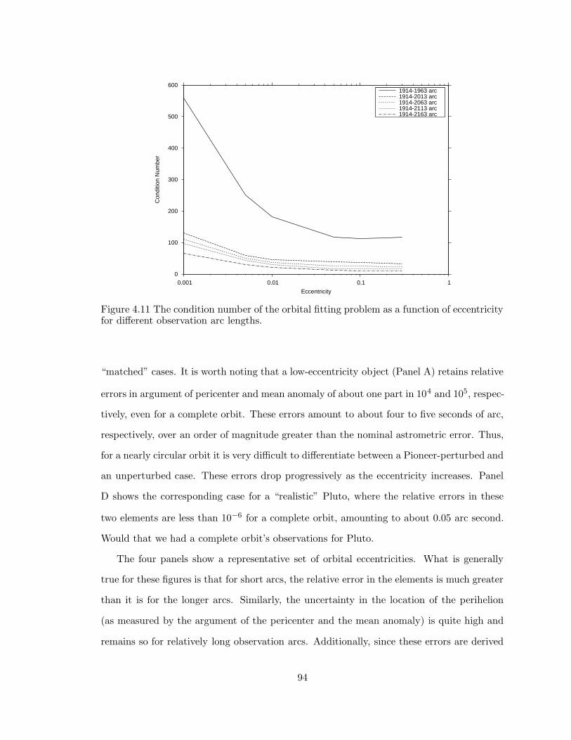
0

100

200

300

400

500

600

0.001 0.01 0.1 1

Con

ditio

n N

umbe

r

Eccentricity

1914-1963 arc1914-2013 arc1914-2063 arc1914-2113 arc1914-2163 arc

Figure 4.11 The condition number of the orbital fitting problem as a function of eccentricityfor different observation arc lengths.

“matched” cases. It is worth noting that a low-eccentricity object (Panel A) retains relative

errors in argument of pericenter and mean anomaly of about one part in 104 and 105, respec-

tively, even for a complete orbit. These errors amount to about four to five seconds of arc,

respectively, over an order of magnitude greater than the nominal astrometric error. Thus,

for a nearly circular orbit it is very difficult to differentiate between a Pioneer-perturbed and

an unperturbed case. These errors drop progressively as the eccentricity increases. Panel

D shows the corresponding case for a “realistic” Pluto, where the relative errors in these

two elements are less than 10−6 for a complete orbit, amounting to about 0.05 arc second.

Would that we had a complete orbit’s observations for Pluto.

The four panels show a representative set of orbital eccentricities. What is generally

true for these figures is that for short arcs, the relative error in the elements is much greater

than it is for the longer arcs. Similarly, the uncertainty in the location of the perihelion

(as measured by the argument of the pericenter and the mean anomaly) is quite high and

remains so for relatively long observation arcs. Additionally, since these errors are derived

94

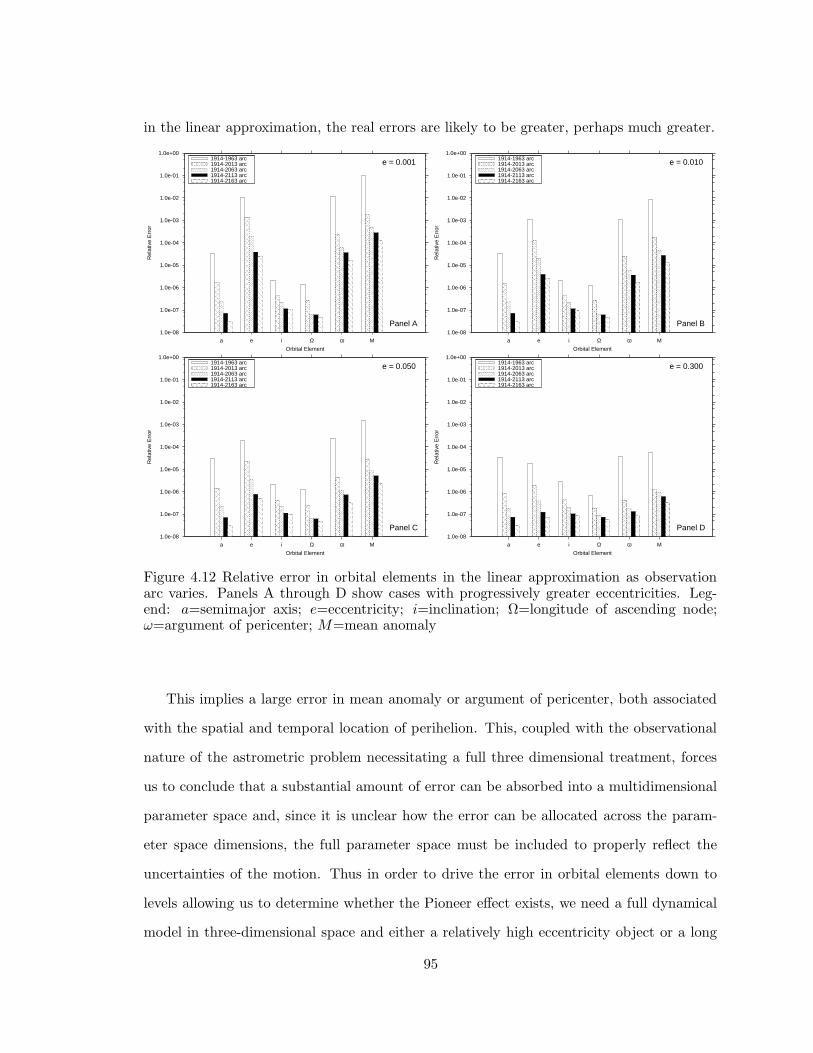
in the linear approximation, the real errors are likely to be greater, perhaps much greater.

1.0e-08

1.0e-07

1.0e-06

1.0e-05

1.0e-04

1.0e-03

1.0e-02

1.0e-01

1.0e+00

a e i Ω ω M

Rel

ativ

e E

rror

Orbital Element

e = 0.001

Panel A


1.0e-08

1.0e-07

1.0e-06

1.0e-05

1.0e-04

1.0e-03

1.0e-02

1.0e-01

1.0e+00

a e i Ω ω M

Rel

ativ

e E

rror

Orbital Element

e = 0.010

Panel B


1.0e-08

1.0e-07

1.0e-06

1.0e-05

1.0e-04

1.0e-03

1.0e-02

1.0e-01

1.0e+00

a e i Ω ω M

Rel

ativ

e E

rror

Orbital Element

e = 0.050

Panel C


1.0e-08

1.0e-07

1.0e-06

1.0e-05

1.0e-04

1.0e-03

1.0e-02

1.0e-01

1.0e+00

a e i Ω ω M

Rel

ativ

e E

rror

Orbital Element

e = 0.300

Panel D


Figure 4.12 Relative error in orbital elements in the linear approximation as observationarc varies. Panels A through D show cases with progressively greater eccentricities. Leg-end: a=semimajor axis; e=eccentricity; i=inclination; Ω=longitude of ascending node;ω=argument of pericenter; M=mean anomaly

This implies a large error in mean anomaly or argument of pericenter, both associated

with the spatial and temporal location of perihelion. This, coupled with the observational

nature of the astrometric problem necessitating a full three dimensional treatment, forces

us to conclude that a substantial amount of error can be absorbed into a multidimensional

parameter space and, since it is unclear how the error can be allocated across the param-

eter space dimensions, the full parameter space must be included to properly reflect the

uncertainties of the motion. Thus in order to drive the error in orbital elements down to

levels allowing us to determine whether the Pioneer effect exists, we need a full dynamical

model in three-dimensional space and either a relatively high eccentricity object or a long

95

observation arc or both.

As observed before, our approach is itself an approximation. A “full dynamical model”

should include not only adjustment of the orbital elements of Pluto, but also simultaneous

adjustment to those of Uranus and Neptune as well. It is only in this way that all the second

order perturbations to the system can be taken into account. However, as observed above,

in order to illustrate the ideas concerned and the weaknesses of the approaches outlined

above, we restrict our attention here to manipulating the orbit of Pluto. This approach will

be justified further in Section 4.3.

4.2.3 How can we assess the quality of an orbital fit?

The problem of assessing model validity and comparing alternative models is huge and any

kind of complete treatment is well beyond the scope of this paper. However, given the

comments above, it is appropriate to offer some observations on this large and interesting

topic.

The issue of goodness-of-fit for models is not a simple one. Often, a χ2 is calculated

and compared to determine which of competing models is the preferred. However, there are

complexities involved. For example, Narsky (2003) discusses goodness-of-fit and points out

that while use of the χ2 statistic as a goodness-of-fit measure for binned data is justifiable

and is often done, it has flaws. He further observes that for unbinned data (such as we have

here), there is no equivalent popular method for measuring goodness-of-fit. Indeed, Heinrich

(2003) gives several examples of problematic goodness-of-fit cases. Similarly, Nat (2006)

advocates investigating the structure of residuals to find patterns, biases, and sytematic

differences between the model and the data.

We can divide metrics for model quality into two broad categories that, although useful,

are certainly not mutually exclusive. First, we can consider what might be termed point

estimates of fit quality. Often, a measure of merit is used that is related to the rms residuals

between the model and the data. Fig. 4.13 compares our rms residuals for various eccen-

tricities. Observations are generated with a Pioneer effect present. One panel of this figure

96

shows the results of fitting the “mismatched” case of the Pioneer-perturbed observations

being fit to a strictly Newtonian gravity model; the other panel shows the corresponding

“matched” case where the gravity model includes a Pioneer perturbation. In both cases

the underlying synthetic observations contain a Pioneer perturbation. The most striking

feature of this figure is how slowly the residual degrades as the arc length increases, espe-

cially for low eccentricity objects. Indeed, until the observation arc is over 100 years long,

there are only small differences in the quality of the fit as measured by rms residuals for

any of the eccentricities evaluated. Even in the “mismatched” case, the rms residual is still

less than half an arc second when the arc is 150 years long. In keeping with the discussion

above about the ill-conditioned nature of the orbital fitting problem, we see that strictly

relying on rms residuals as a measure of merit for model selection can be problematic.

Another measure of merit that is sometimes invoked is the uncertainties in the orbital

elements themselves. The orbital fitting process automatically provides mathematically

well-justified estimates of the elements, although these are in a linear approximation that

has its own difficulties since the orbital fitting problem is intrinsically nonlinear. This

approximation provides error estimates similar to those shown in Fig. 4.12. Across the

eccentricities shown, there is substantial error spread throughout the parameter space. In

particular, it might be instructive to compare Panels A and D in Fig. 4.12. In Panel A,

a very low eccentricity case, the errors in semimajor axis, inclination, and longitude of the

ascending node drop to a level allowing seven or eight significant digits to be present in the

corresponding element values. At the same time, however, the uncertainties in eccentricity,

argument of the pericenter, and mean anomaly remain relatively large. In the case with the

largest eccentricity evaluated, Panel D shows the uncertainty to be more uniformly spread

across elements. Trading off the uncertainties of one element against those of another to

compare two models is therefore at best arbitrary and could be misleading.

Position error in the sky plane is yet another point metric for fit quality. In this case,

uncertainties in the orbital elements are mapped directly onto the sky. Here, all the com-

ments above about the uncertainty of the elements are valid, plus the observation that

97

0.00

0.50

1.00

1.50

2.00

2.50

3.00

0 50 100 150 200 250 300

RM

S e

rror

of o

rbita

l fit

(arc

sec)

Observation Arc Length (year)

Panel A

e = 0.300e = 0.200e = 0.100e = 0.050e = 0.010e = 0.005e = 0.001

0.00

0.50

1.00

1.50

2.00

2.50

3.00

0 50 100 150 200 250 300

RM

S e

rror

of o

rbita

l fit

(arc

sec)

Observation Arc Length (year)

Panel B

e = 0.300e = 0.200e = 0.100e = 0.050e = 0.010e = 0.005e = 0.001

Figure 4.13 Rms residual of orbital fit as observation arc length varies. Panel A shows the“mismatched” case where the observations are fit to a gravity model not containing thePioneer effect. Panel B shows the “matched” case where the same observations are fit to agravity model that includes a Pioneer effect perturbation.

98

the mapping from the six-dimensional space of orbital elements to the two-dimensional sky

plane is highly degenerate; many sets of elements can map to the same region of sky. Thus,

the sky plane position, by itself, can have problems as a point measure of model fit quality.

In particular, comparing the nominal solution for two models can result in a large error

volume about the calculated positions of objects.

All three approaches to providing point estimates of model fit quality have one common

weakness. They are all based on a linearized form of the orbital fitting problem and make

the assumptions associated with least squares fitting like normally distributed errors, inde-

pendence, and no bias or systematic errors. Possibly the biggest manifestation of this is

that we should not expect to be able to accurately extrapolate very far beyond the available

observation arc unless there is at least a full orbital revolution’s volume of data and even

then, extrapolation is dangerous.

A possibly better approach to comparatively assessing model alternatives is to use some

type of global comparison. Of broadest applicability in this context is the idea of testing for

the normality of the residuals between the model and the data. The overall basis for these

tests is to look at the structure of the residuals and to perform statistical tests for lack of

fit (see, for example, Nat (2006, Section 4.4.4.6)). The basis for these tests is to search for

patterns, biases, and systematic differences between the model and the data.

Another approach that could be used to address the global quality of fit is to use boot-

strap techniques. This approach could involve, as done here, synthesizing observations

whose error characteristics reflect those found actual observations and then using the syn-

thetic observations to assess actual variations in the fit quantities. Another approach of

this sort would be to remove some of the data from the fit and see how the fitted solution

extrapolates to the times that were removed. A similar approach would be simply to re-

move data randomly from the observation set and analyze the resulting variations in fitting

parameters.

One form that this approach could take would be to conduct a full Bayesian analysis

99

of competing models. The distributions of orbital elements resulting from synthetic obser-

vations that arise from a Monte Carlo process could be used to compare the probability

of obtaining the observations in light of the competing models (see, for example, Gregory

(2005); Jaynes and Bretthorst (2003); Sivia and Skilling (2006)). Although beyond the

scope of this chapter, the findings discussed here show that there are not currently enough

data to warrant this type of analysis; however, the advent of Pan-STARRS and LSST will

change that situation in the near future.

4.3 Discussion

In the analysis described above we first showed that one cannot simply take orbital elements

resulting from the fit of observations to a particular force model and use them to predict

positions resulting from motion under the influence of another force. Rather, we must refit

the orbits to the observations under the new force model. In the case of Pluto, this produces

a well-fitting orbit that is indistinguishable in a practical sense, at least as long as the

observation arc is short enough, from the unperturbed motion. Thus, without redetermining

the elements we cannot make sweeping generalizations about whether or not the outer

planets’ orbits show that the Pioneer effect does or does not exist.

Similarly, although making simplifying assumptions about a physical situation in order

to draw conclusions is a time-honored theoretical mode of attack, if the physical model is

oversimplified we can be misled into erroneous conclusions. As seen above, in an obser-

vational context, both observer position and observational errors lead to the necessity of

introducing the third spatial dimension with its associated degrees of freedom. If we do

not keep an appropriate number of degrees of freedom, the problem can be oversimplified

too much and mislead us into unwarranted conclusions. In particular, we must take care in

using such a simplified model to conclude that the Pioneer effect does not exist.

Once again, it should be emphasized that our approach is itself an approximation.

To properly conduct an analysis of the sort outlined here, the orbital parameters of the

entire system of outer planets should be included. This would bring into the calculation

100

0.0

0.2

0.4

0.6

0.8

1.0

1.2

1.4

1.6

1900 1950 2000 2050 2100

Acc

eler

atio

n/P

ione

er a

ccel

erat

ion

Time (year)

Uranus-PlutoNeptune-Pluto

Figure 4.14 Gravitational acceleration exerted by Uranus and Neptune on Pluto as a func-tion of time.

all second order perturbations. However, we have taken a simplified approach and believe

it accurately and fairly addresses the uncertainties in the orbit of Pluto. One reason we

believe our simplified approach is valid is illustrated in Fig. 4.14.

Fig. 4.14 shows the force per unit mass (in units of the Pioneer acceleration) exerted by

Uranus and Neptune at Pluto’s position over the period of time we have considered. Perhaps

surprisingly, due to the relative positions of the planets in their orbits, Neptune exerts less

force on Pluto than Uranus over most of this period. The magnitude of the force is of the

order of the Pioneer acceleration for both planets. If the Pioneer effect exists, we would

expect the orbital elements of Uranus and Neptune to change, but their positions would

change by very little. The magnitude of the forces they exert on Pluto would therefore

change by an amount much less than the current magnitude of those forces. Thus, we argue

that the approach used in this paper, while not as accurate as a full second order calculation

involving all the outer planets, is accurate enough for our purposes.

Given the comments above, how then are we to compare alternative models? There are

a number of methods that we can use to compare and assess models and their results. In

101

the orbit fitting context, these have been discussed above in terms of point estimates and

global estimates of goodness of fit. The simplest point estimate is to simply calculate the

rms residual of the fit compared with the input observations. However, as we’ve seen, the

ill-conditioned nature of the orbital fitting problem can sometimes make the residual a poor

candidate for this role. Errors, in the linear approximation, to the orbital elements can be

assessed to determine the quality of the fit. Further physical insight can be gathered from

inspecting the sky position errors that result from element errors. Global assessments of

model fit primarily revolve around the normality of residuals. There are lack of fit tests that

can be used to test the residuals and determine if there are any indications of a deficient

model. Generally, a lack of fit is manifested as patterns, biases, and systematic variations

in the residuals, which would indicate a poorly fitting model.

Which of these metrics is best? The reality is that determining the quality of a model

and comparing model effectiveness is a complex problem. We need all these measures

of model fit. Statistical tests should be performed comparing predicted positions, taking

proper account of the associated errors, to test the hypothesis that the positions predicted

under the two dynamical models are different. Only in this way can the existence of a

perturbation like the Pioneer effect be falsified through astrometric methods.

As discussed earlier, Pluto is very interesting in that orbital fits to the two gravity models

show deviations in predicted position that are probably detectable if the entire observation

arc consisted of reliable measurements. However, prior to about 1960, there is a significantly

greater dispersion in residuals that at later times. Only about half of Pluto’s motion since

its discovery has been the result of systematic and organized observing campaigns (Gemmo

and Barbieri, 1994). What adds special interest, however, is that because of its relatively

large eccentricity Pluto is likely to show differences in position predictions for the two gravity

models in the relatively near future as more observations are accumulated.

102

4.4 Conclusions

The analysis described above shows two major things. First, we must fit observations to a

particular dynamical model and adjust orbital elements before predicted positions on the sky

can be compared. Orbital parameters are derived from observations which have associated

an unavoidable error. The determination of orbits is a model fitting process which has

its own associated error sources. Extrapolating sky positions very far past the end of an

observation arc can result in predicted observations becoming inaccurate so rapidly as to be

worthless. The implication of these findings is that “matched” and “mismatched” gravity

models cannot be distinguished on the basis of observable sky positions for observation arc

lengths similar to those currently obtaining for Pluto.

Similarly, in order to draw conclusions about differences in position in the sky, we

must be careful not to oversimplify the dynamical model used to draw the conclusions.

Suppressing degrees of freedom in the dynamics simplifies the orbital determination problem

to just such a degree. The orbital determination problem is nonlinear and the customary

solution methods are approximations. Thus, any missing or ignored degrees of freedom can,

if present, conceal dynamical effects associated with differing gravity models; we are forced

to make use of the full dimensionality of the dynamical problem. In particular, a substantial

amount of variation can be absorbed into a multidimensional parameter space and the full

parameter space must be considered to properly reflect differences in motion of the outer

planets due to the Pioneer effect.

The problem with the simplified approach is a two-headed one. First, the orbital fitting

problem is inherently nonlinear and is normally solved in the linear approximation. Even

if not mathematically chaotic, the system of equations is sensitively dependent upon initial

conditions. Thus, small changes in elements can result in large changes in predicted position

outside the range of observations. This sensitivity is exacerbated by the problem of a short

observation arc. The length of the entire observational archive for Pluto is less than about

one-third of a complete revolution. Together, these factors conspire to potentially generate

large errors outside the observation arc, while increasing the length of the observation arc

103

can markedly reduce error over the whole of the arc and even beyond it.

We must conclude that we do not know the orbit of Pluto as well as we might have

thought. We must continue to perform astrometry on it in order to be able to comment

on the accuracy with which we know its orbit. Using current data, we cannot assert that

the motion of Pluto demonstrates that the Pioneer effect does not exist. That jury is still

out. Of course, this does not mean that the Pioneer effect exists. It does mean that we

cannot deny the existence of the Pioneer effect on the basis of motions of the Pluto as

currently known. Further observations are required before such an assertion can be made

with confidence.

It should again be emphasized that our approach is itself an approximation. The dy-

namical system that should be analyzed to provide a comprehensive answer to the question

of the detectabilty of the Pioneer effect should include not only adjustment of the orbital

elements of Pluto, but also simultaneous adjustment to those of Uranus and Neptune as

well. It is only in this way that all the second order perturbations to the system can be

taken into account. Our approach here, however serves to illustrate the ideas concerned

and the weaknesses of the approaches outlined above.

Finally, it should be pointed out that, in addition to the observations of individual

objects discussed in this paper, there are other related approaches to assessing gravity in

the outer Solar System. For example, recently Wallin et al. (2007) have investigated the use

of ensembles of Trans-Neptunian Objects (TNOs) to ascertain whether their motion reflects

unknown additional perturbations and showed that the Pioneer effect was not consistent

with the motion of TNOs. On the other hand, in the area of the observation of individual

objects as discussed in this paper, the advent of Pan-STARRS and LSST in the next several

years should provide sufficient data to determine whether the motion of outer Solar System

bodies reflect the action of unknown forces. This determination should occur over time

frames discussed in this paper. However, a combination of the techniques of Wallin et al.

(2007) and the considerations presented here should provide definitive answers more quickly.

104

Chapter 5: Comets as Gravity Probes

There is another group of objects that might provide a vehicle for assessing the existence of

the Pioneer effect through astrometry: the comets. Following the same general theme, we

will now briefly look at them. Can they provide a vehicle for investigating the gravitational

field in the outer Solar System?

Previously, we have emphasized the necessity of using complicated tools to investigate

complicated Solar System dynamics. Here, we will take a slightly different tack. Comets

are distinguished by the source of their comae and tails: outgassing. To the extent that

any dynamic effects of cometary outbursts cannot be quantified, small perturbations like

the Pioneer effect cannot be distinguished.

Thus, the purpose of this chapter is to investigate whether outgassing prevents the use

of comets for exploring gravity in the outer Solar System.

The remainder of this chapter is divided into four sections. Section 5.1 will discuss the

methodology employed to make the assessment. Section 5.2 discusses the results of the

analysis. Finally, Section 5.3 provides a discussion of the results and Section 5.4 presents

conclusions.


The approach taken in this chapter is to model the orbits of comets in the outer Solar

System by means of Newtonian gravity and two-body, planar motion. We will consider the

Sun’s field to be spherically symmetric and will ignore the gravitational perturbations due

to planets and the larger asteroids on the motion of the bodies of interest. While the impor-

tance of these effects is recognized, especially during the conduct of precision astrometry,

they do not need to be considered in detail in the beginning of assessing the feasibility of

105

our approach. Initially, we only explore the perturbative effects of the Pioneer effect on

comet orbits. Since these effects, to first order, are linearly independent of other orbital

perturbations (e.g., perturbations due to planets), the latter can be safely ignored. Other

perturbations, for example the anisotropic thermal radiation giving rise to the Yarkovsky

Effect for asteroids, Non-Gravitational Forces (NGF) due to outgassing for comets, General

Relativity, and the Pioneer effect will be addressed as appropriate.

The general approach used is to model the motion of bodies of interest subject to the

perturbing forces of interest and to compare the heliocentric angular differences between the

comets in the different cases. The time evolution of these angular differences is considered

along with the distances of the bodies and the precision with which their orbits are known

to determine whether or not the effects of the perturbations can be detected and whether

they can shed any illumination on the nature of the mass distribution in the outer Solar

System.

A standard implementation of the Runge-Kutta-Fehlberg integrator is used to deter-

mine the orbits of the objects of interest. The particular routine used was RKF45 and was

obtained from the National Institute of Science and Technology GAMS web-site.1 While

recognizing that Runge-Kutta integrators are not generally known for their high precision

results, they are adequate for the feasibility investigation conducted here since we are ex-

amining individual orbits rather than systematic long-term trends.

The approach outlined above is used for sample selection and provides a vehicle for first

order exploration of the effects that might be observed if the Pioneer effect were real. This

approach would be complete in an ideal world, but we must perform our science in a messier

reality. As observed previously, because the motions of minor planets are complex, we really

need to carry our analysis one step further. Since unavoidable observational errors and the

motions of many perturbing bodies influence the dynamics of minor planets, the general

approach towards understanding their motion involves determining orbital elements in such

a way as to minimize discrepancies between observation and prediction. In our context,

1 Available from NIST at http://gams.nist.gov.

106

the problem is that adjustment of orbital parameters might allow motion perturbed by the

Pioneer effect to be masked completely and might make the Pioneer effect unobservable in

practice. For example, a change in orbital eccentricity might allow motion pertubed by the

Pioneer effect to be explained completely in terms of a non-Pioneer model. In this case,

there would be no way to show the existence of the Pioneer effect because the effect would

be concealed beneath the variation resulting from measurement errors. However, as we will

see below, for comets, the simpler approach is warranted.

5.1.1 Non-Gravitational Forces

Comets also suffer orbital perturbations due to Non-Gravitational Forces (NGF) that pre-

sumably result from outgassing. The NGF are parametrized in a standard way (Marsden et

al., 1973) and departures from osculating orbital elements provide estimates of the values of

acceleration experienced by the comet. These forces have a substantial effect on the orbital

parameters of comets, amounting to as much as several days difference in the predicted

time of perihelion passage, a difference comparable to that produced by the Pioneer effect.

This standard parametrization is of a statistical nature. Since there is a variation in NGF

from orbit to orbit, presumably as the comet’s “dirty snowball” nature changes with mul-

tiple passes by the Sun, it is difficult or impossible to predict the exact motion of comets

throughout their orbits.

5.1.2 Comet Sample Selection

There are surprisingly few comets whose orbits are both known sufficiently accurately to be

of interest and whose aphelion distance is greater than our assumed Pioneer effect cutoff.

Additionally, because of their extended natures, it is difficult to unambiguously determine

the center of light of the comet (and even that is not necessarily indicative of the actual

location of the nucleus). Thus, determining the precise location of comets so that their

orbits can be determined accurately is quite difficult.

Since there is a variation in NGF from orbit to orbit, presumably as the comet’s “dirty

107

Table 5.1 Orbital parameters of comets susceptible to the Pioneer Effect.

Comet a e T Q A

1P/Halley 17.834 0.967143 75.32 0.586 35.08212P/Pons-Brooks 17.121 0.954812 70.75 0.774 33.46913P/Olbers 16.907 0.930297 69.52 1.178 32.63523P/Brorsen-Metcalf 17.069 0.971952 70.52 0.479 33.66038P/Stephan-Oterma 11.248 0.860022 37.72 1.574 20.921109P/Swift-Tuttle 26.092 0.963226 133.28 0.960 51.225122P/deVico 17.681 0.962709 74.35 0.659 34.702

Notes: a is semimajor axis in AU, e is eccentricity, T is period inyears, Q is perihelion distance in AU, and A is aphelion distance inAU.

snowball” nature changes with multiple passes by the Sun, we consider only comets with

nearly three perihelion passages resulting from nearly two complete orbits and that pass

more than 20 AU from the Sun. The Jet Propulsion Laboratory’s Horizons ephemeris sys-

tem (Giorgini et al., 1996) contains 522 such comets, including those with orbital elements

determined at multiple epochs. This list was winnowed in a straightforward way by choos-

ing, in those cases where elements were determined for multiple epochs, the most recent

epoch whose data arc included nearly two complete orbits about the Sun. Comets with

eccentricities greater than or equal to unity were also excluded. Table 5.1 shows selected

orbital elements of the resulting short list of seven candidate comets satisfying these criteria.

5.2 Results

As early as 1823 secular accelerations of comets were observed (Encke, 1823), and various

hypotheses were proposed to explain them. Beginning in 1968, Marsden and his collab-

orators began a series of papers addressing the issues associated with NGF and comets.

Beginning by establishing that short period comets experience both secular accelerations

and decelerations (Marsden, 1968), continuing with the development of an empirical model

of the NGF (Marsden, 1969), and finally culminating in a physically justified model for

NGF (Marsden et al., 1973) that is founded in the “dirty snowball” or icy-conglomerate

108

cometary model (Whipple, 1950). Investigations along these lines continue. Short period

comets are relatively easy to observe and to establish NGF parameters, and even to study

how the accelerations change from orbit to orbit (Yeomans, 1994). More recently, long-

period comets were investigated using positional observations only and corroborated the

good agreement of the Marsden model with observations (Krolikowska, 2004).

The standard model of NGF contains three parameters, generally denoted by A1, A2,

and A3. These are components of the nongravitational acceleration in a radial direction,

in a transverse direction in the orbital plane, and normal to the orbital plane, respectively.

The magnitude of the nongravitational acceleration close to the Sun is surprisingly large.

At a distance of 1 AU, and for a fiducial value of A1 of 10−9 AU day−2, the nongravitational

acceleration is approximately 2 × 10−5 cm sec−2, compared with the acceleration due to

the Sun’s gravity of 0.6 cm sec−2. However, the standard model of NGF drops rapidly

with increasing distance. By the time a comet is 20 AU from the Sun, the nongravitational

acceleration decreases to approximately 3×10−28 cm sec−2, an unmeasurable quantity. This

acceleration magnitude is compared with 1.5 × 10−3 cm sec−2 from the Sun’s gravity and

8.74 × 10−8 cm sec−2 for the Pioneer effect.

The normal component (A3) is generally found to be less significant than the others

and its value is often indeterminate. The NGF parameters are empirically determined and

are comet-specific. The JPL Horizons ephemeris system (Giorgini et al., 1996) provides the

values for the radial and transverse accelerations for our candidate comets that are shown in

Table 5.2. Also shown in this table is the change in orbital period due to the NGF, typically

of the order of days, with the perturbed orbital periods generally being more lengthy than

the corresponding Keplerian period.

The orbital periods of comets subjected to the Pioneer effect are systematically shorter

than the corresponding Keplerian period. As also shown in Table 5.2, the typical change

in orbital period due to the Pioneer effect is of the order of days; that is, the same order

of time as the NGF-induced period change. These changes are small and correspond to no

more than a 0.05 percent change in orbital period in both cases.

109

Table 5.2 Change in comet orbital period because of Pioneer Effect and NGF.

Change in Period Radial NGF (A1) Angular NGF (A2)

Comet Kepler-Pioneera Kepler-NGFa With PEb No PEc With PEb No PEc

1P/Halley 4.7 -2.8 1.33 0.27 1.33 1.5512P/Pons-Brooks 4.0 4.7 -0.183 -1.02 -0.183 -2.7113P/Olbers 3.9 14.1 11.3 9.45 11.3 6.4923P/Brorsen-Metcalf 3.9 -6.6 1.57 2.25 1.57 -5.3338P/Stephan-Oterma 0.3 -0.2 1.93 1.27 1.93 -0.315109P/Swift-Tuttle 24.8 0.0 3.43 0.0 3.43 0.0122P/deVico 4.6 0.0 0.966 0.0 0.966 0.0

Notes: Times are given in days, the radial nongravitational parameter (A1) is given in units of 10−9 AU day−2, and

the angular nongravitational parameter (A2) is given in units of 10−10 AU day−2.

a Positive numbers indicated the Keplerian orbital period is longer by the indicated number ofdays.b Indicates “With the Pioneer effect.”c Indicates “Without the Pioneer effect.”

Although the changes in orbital periods are of the same magnitude for both the Pioneer

effect and the NGF, they are in opposite directions, one serving to increase the period,

the other decreasing it. This, coupled with the physically well-founded justification for the

standard NGF model makes it desirable to investigate whether the potential existence of

a Pioneer effect has any implication for the NGF model. Generally, the magnitude of the

transverse NGF parameter (A2) is about one-tenth of the value of the radial parameter

(A1) (Marsden et al., 1973). If we constrain the value of A2 to be of that value, and

allow the radial acceleration to vary parametrically, we can obtain a new value of the NGF

parameter that allows the orbital period to remain at its proper value even when the Pioneer

effect influences the orbits. The resulting values for the NGF parameters are also shown in

Table 5.2. There is no statistically significant difference between the distributions of NGF

parameters with and without the Pioneer effect.

Although NGF are generally not significant far from the sun, there remain a substantial

number of outgassing episodes that have been observed at large distances. These have been

detected in a number of comets, including Halley (Gronkowski and Smela, 1998; West et al.,

1991), Chiron (Elliot et al., 1995; Sekiguchi et al., 1998), and Ikeya-Seki and Schwassmann-

Wachmann 1 (Gronkowski and Smela, 1998). The framework of the standard NGF model

provides a convincing explanation for these episodes (Prialnik and Bar-Nun, 1992; Womack,

110

2000). However, calculations of momentum transfer in these distant outbursts suggest that

the eruptions are far less dynamically significant at large distances from the Sun than they

are at smaller distances (Hainaut et al., 1995).

Since the magnitude of changes in cometary orbital periods associated with the Pioneer

effect and NGF are of the same magnitude, changes in NGF parameters can have an effect

close to the sun that can mask changes in period due to the Pioneer effect. Thus, we

must conclude that comets do not represent ideal candidates for investigating the Pioneer

effect: Given the existence of NGF, departures from the ephemeris might not be a sufficient

condition for the Pioneer effect to exist. Nevertheless, while not ideal, comets might provide

a useful vehicle for observational verification of the Pioneer effect. In any event, the high

eccentricities of comet orbits compared with those of planets make it clear that the Pioneer

effect will manifest itself much more clearly in the former case than in the latter.

5.3 Discussion

We have previously discussed the orbits of comets under the influence of the Pioneer effect

and found that the magnitude of the effect is similar to that of the customary NGF used

to calculate ephemerides. This approach is similar to a “kinematic” approach, wherein

we explore features of the motion without regard for its specifics. However, a “dynamic”

assessment, incorporating the current location of comets in their orbits is now of interest in

order to determine whether the Pioneer effect is observationally detectable.

Of our seven comet candidates, nearly all are currently beyond 20 AU and thus subject

to the Pioneer effect as defined in this dissertation. The single exception is just inside 20 AU,

moving towards the Sun, and has recently left the Pioneer effect behind. These bodies have

all been subjected to the Pioneer effect for some time and their current positions are already

perturbed relative to their ephemerides without the Pioneer effect. The resulting angular

differences range from −7.2 to +1.4 seconds of arc, with negative numbers indicating the

Pioneer-perturbed orbit is ahead of the unperturbed motion in terms of true anomaly. The

initial discrepancy is shown in Table 5.3 for each comet, along with other data on the current

111

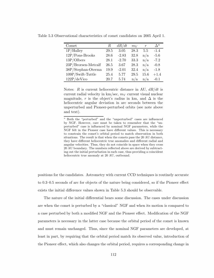
Table 5.3 Observational characteristics of comet candidates on 2005 April 1.

Comet R dR/dt mV r ∆a

1P/Halley 29.5 3.05 28.3 5.5 -1.412P/Pons-Brooks 28.6 -2.83 32.8 n/a -5.613P/Olbers 28.1 -2.70 33.3 n/a -7.223P/Brorsen-Metcalf 26.5 3.67 28.3 n/a -0.838P/Stephan-Oterma 19.9 -2.01 32.4 n/a -1.8109P/Swift-Tuttle 25.4 5.77 29.5 15.6 +1.4122P/deVico 20.7 5.74 n/a n/a -0.1

Notes: R is current heliocentric distance in AU, dR/dt iscurrent radial velocity in km/sec, mV current visual nuclearmagnitude, r is the object’s radius in km, and ∆ is theheliocentric angular deviation in arc seconds between theunperturbed and Pioneer-perturbed orbits (see note aboveand text).

a Both the “perturbed” and the “unperturbed” cases are influencedby NGF. However, care must be taken to remember that the “un-perturbed” case is influenced by nominal NGF parameters, while theNGF felt in the Pioneer case have different values. This is necessaryto constrain the comet’s orbital period to match observation in bothsituations. The result is that when the comets pass the 20 AU distance,they have different heliocentric true anomalies and different radial andangular velocities. Thus, they do not coincide in space when they cross20 AU boundary. The numbers reflected above are derived by subtract-ing out the initial perturbation in each case, thus providing a coincidentheliocentric true anomaly at 20 AU, outbound.

positions for the candidates. Astrometry with current CCD techniques is routinely accurate

to 0.3–0.5 seconds of arc for objects of the nature being considered, so if the Pioneer effect

exists the initial difference values shown in Table 5.3 should be observable.

The nature of the initial differential bears some discussion. The cases under discussion

are when the comet is perturbed by a “classical” NGF and when its motion is compared to

a case perturbed by both a modified NGF and the Pioneer effect. Modification of the NGF

parameters is necessary in the latter case because the orbital period of the comet is known

and must remain unchanged. Thus, since the nominal NGF parameters are developed, at

least in part, by requiring that the orbital period match its observed value, introduction of

the Pioneer effect, which also changes the orbital period, requires a corresponding change in

112

NGF parameters in order to leave the orbital period unaltered. For the sake of brevity, in

this section only, we will refer to the nominal NGF case as “unperturbed” and the modified

NGF plus Pioneer effect case as “perturbed.”

Another interesting aspect of this initial discrepancy is that recent observations of

1P/Halley show it to be approximately 1.4 seconds of arc behind its ephemeris position

(Hainaut et al., 2004), while these simplified calculations show it to be about 1.2 seconds

of arc behind at the time of the observations, a remarkably similar quantity. Although

differences on the order of a second of arc potentially can be understood in terms of errors

in the astrometry, the idea that perturbations due to the Pioneer effect contribute is worthy

of additional investigation.

If the current position of the candidate comets is corrected for this initial discrepancy,

and the unperturbed and Pioneer-perturbed comets are made to coincide at the current

epoch, we can investigate the rate at which the angular deviation grows from the present.

Thus, Figure 5.1 shows the heliocentric angular deviation of each comet from a starting

point of 2005 April 1. Recall that the standard NGF parameters shown in Table 5.2 are

generally positive, implying an outward-directed NGF. Thus, the NGF generally acts to

lengthen the orbital period of comets by pushing them out to greater aphelion distances.

As time progresses, the perturbed orbit falls more and more behind one not influenced by

NGF. However, by the time the Pioneer effect comes into play, the NGF are essentially

nonexistent. Once they are felt, the acceleration due to the Pioneer effect serves to lessen

the aphelion distance and increases the angular velocity of the comet. Thus, Figure 5.1

shows angular deviations that grow in the negative direction, leading us to expect the

Pioneer-perturbed comets to get progressively more and more ahead of the unperturbed

positions as time progresses.

Figure 5.1 would seem to indicate that comets would provide fertile ground for deter-

mining whether the Pioneer effect really exists, with angular deviations reaching detectable

levels as soon as two to three years from now. However, these angular differences are con-

sistent with current astrometric errors for measurements of this type. More importantly,

113

-1.0

-0.8

-0.6

-0.4

-0.2

0.0

0 1 2 3 4 5

Ang

ular

Dev

iatio

n (O

-C)

(arc

sec)

Elapsed Time (yr)

1P/Halley12P/ZPons-Brooks13P/Olbers23P/Brorsen-Metcalf38P/Stephan-Oterma109P/Swift-Tuttle122P/deVico

Figure 5.1 Heliocentric angular deviation between modified NGF-perturbed comet candidateorbits and those perturbed by the Pioneer effect. The elapsed time is that from 2005 April1. The angular differences shown are consistent with current astrometric errors.

Table 5.3 also shows the current nuclear magnitude of the comets; the brightest currently

has a magnitude of something over 28, while the faintest is dimmer than magnitude 33.

Unfortunately, it is extremely difficult to detect objects this faint. Recent observations

of 1P/Halley have detected the comet at a distance of over 28 AU and at a visual magnitude

of more than 28 (Hainaut et al., 2004). These observations are part of an ongoing campaign

to monitor 1P/Halley after perihelion, in an effort to define the orbit and allow early pre-

perihelion recovery (Hainaut et al., 1995; West, 1990; West and Jorgensen, 1989; West et

al., 1991). The observations represent the greatest distance and the greatest magnitude

of any cometary observation. The three 8.2 meter Very Large Telescopes at the European

Southern Observatory’s Paranal site were used simultaneously for a total exposure of 32,284

seconds in order to achieve this remarkable feat.

The current magnitudes of the candidate comets, coupled with the difficulties associated

with NGF, outlined previously, force us to conclude that comets do not currently provide

a good opportunity for investigating the Pioneer effect. However, continuing cometary

114

observations such as the long term program at the ESO, might provide insight over time,

especially as target comets approach aphelion. However, the idea that the Pioneer effect

and the standard NGF model do not conflict with one another represents an important

conclusion.

Nevertheless, referring back to Table 5.3 provides motivation for an interesting observa-

tion about the Swift-Tuttle comet. One of the difficulties associated with determining NGF

for long period comets is simply that they have not been observed for a significant number

of revolutions. There are some exceptions. For example, using ancient Chinese records,

apparitions of 1P/Halley have been convincingly connected from its 1986 appearance back

28 revolutions, over more than 2000 years (Kaing, 1972). The important finding here is that

the comet returned consistently about four days late over this entire span. Additionally,

it had no significant change in magnitude over that interval. This orbital period change

is remarkably close to the magnitude of the change due to the Pioneer effect or to NGF.

If we suppose that the relatively constant magnitude is indicative of a relatively constant

amount of outgassing, we may further imagine that there has been relatively little change

in the NGF as well. 1P/Halley thus demonstrates that the motion of comets can remain

uniform over long intervals.

Swift-Tuttle’s motion is known over long periods also. Although its orbit has been

traced back for more than 2000 years (Yau et al., 1994), its motion is consistent with no

NGF, even though a well-developed coma shows this comet outgasses. Further, there is no

evidence of any change in its absolute magnitude over this entire interval. The comet has a

relatively long period and goes further into the Pioneer effect region than any other of our

comet candidates, thus the effect of the Pioneer effect on its orbital period is the largest

of our candidates: Swift-Tuttle’s period is lessened by almost 25 days in the absence of

other perturbations. It is certainly a provocative speculation that Swift-Tuttle’s outgassing

causes NGF that fortuitously change the orbital period in the right way to make NGF

seem to be nonexistent. Thus, if the Pioneer effect is present, the altered NGF required to

increase the orbital period to its recognized value are completely reasonable and in no way

115

unusual. Recognizing the difficulties with a bright comet not having any NGF has resulted

in speculations that Swift-Tuttle is much more massive than comet Halley (Yeomans, 1994).

While possible, the interesting idea that the Pioneer effect could imply that Swift-Tuttle is

a less unusual body is worthy of further investigation.

5.4 Conclusions

This chapter shows that comets, although seemingly providing a potential observational

vehicle for investigating the Pioneer effect, are by no means ideal for this purpose. Although

possessing many of the qualities that made asteroids useful for this purpose, for example,

because they have a large mass and are large and bright enough to observe for possibly

satisfactorily long intervals.

However, comets possess many characteristics that make them a marginal candidate for

assisting us in our quest. Generally, comets are of small size and have a low albedo. This

makes them difficult to observe at distances from the Sun where the Pioneer effect plays a

role. Also problematic is the fact that comets can be extended sources. Locating the center

of light of a comet image can present more problems than nominal asteroids.

In terms of the existence of the Pioneer effect, perhaps the most important thing comets

have to say is that if the Pioneer effect exists, the impact on the motion of comets would

not contradict the physically well-motivated NGF model. Although the NGF model pa-

rameters would have to change, the changes would result in model parameter values that

are completely reasonable.

Notwithstanding the poor prospects of comets providing astrometric data showing the

existence or non-existence of the Pioneer effect, they do have some interesting charac-

teristics. Continuing observations such as those undertaken at the ESO (Hainaut et al.,

2004) might provide insight over time into vagaries in their motion, especially as target

comets approach aphelion. ESO observations also provided the provocative result that

comet 1P/Halley is approximately 1.4 seconds of arc behind its expected ephemeris posi-

tion. The idea that perturbations like the Pioneer effect could contribute to this discrepany

116

is worthy of further investigation.

Another issue that might be worthy of further investigation is the orbit of comet

109P/Swift-Tuttle. Because of its brightness, Swift-Tuttle is assumed to be large. Its

NGF parameters are also zero. The idea of a large comet with substantial outgassing flies

in the face of the physical justification for the NGF. The idea that Swift-Tuttle’s outgassing

causes NGF that fortuitously change the orbital period in the right way to make NGF seem

to be nonexistent is provocative. However, the idea that the Pioneer effect could imply that

Swift-Tuttle is a less unusual body is worthy of further research.

117

Chapter 6: Impact of LSST and Pan-STARRS

When published, the material presented in Chapter 3 (Page et al., 2006) investigated the

possibility of using minor planets to assess gravity in the outer Solar System. That paper was

mostly devoted to the use of astrometry of asteroids to test the inverse square law of gravity

in the outer Solar System and the potential use of such observations to ascertain the reality

of the Pioneer effect (a constant, sunward, radial acceleration that has resisted conventional

explanation). This material showed that a sustained, although not intensive, observation

campaign could discern whether the Pioneer effect perturbed the orbits of properly selected

asteroids in no more than 20 years.

The need for more observations runs afoul of the scarcity of available time on instruments

appropriate to this type of astrometry program. However, the advent of facilities such

as Pan-STARRS (Jewitt, 2003) and LSST (Sweeney, 2006) places observation programs

such as that proposed in Chapter 3 in a new light. Pan-STARRS will provide coverage

of the available sky three times during each dark moon period and LSST is intended to

provide complete coverage of the available sky every three nights. The very high observation

cadences planned for these remarkable instruments place the assessment of gravity in the

outer Solar System by astrometric means within reach independent of telescope availability.

We will use the Pioneer effect as an exemplar of a gravitational perturbation, but the

method described here is applicable to any other gap in our knowledge or understanding

of the gravitational field in the outer Solar System. There is not a great deal of literature

on this topic, and most is devoted to looking at outer planets, which are generally very

low eccentricity bodies. The problems associated with using the outer planets to measure

gravity at intermediate scales will be dealt with elsewhere, and this paper’s primary purpose

is to investigate the relationship of observations to orbital parameters such as semimajor

118

axis and eccentricity and the length of the observation arc leading to the determination of

the orbital elements.

It is important to recognize explicitly the question being asked in this analysis. We

are parametrically varying two orbital elements: semimajor axis and eccentricity. In all

cases, these parameters are treated as being initially known exactly. The question we ask

in this chapter is, given a reality containing an orbiting body with given semimajor axis

and eccentricity, what will happen if we compare observations made subject to a Newtonian

model of gravity with ones made that include additional perturbations. Thus, as described

below, we generate simulated observations arising from the same initial conditions (e.g.,

orbital elements) and the two gravity models, and compare the predicted locations in the

sky to see what observationally detectable position differences result in light of observation

and other errors. The converse problem of understanding what variations in orbital elements

lead to distinguishable sky positions presents different challenges and will be dealt with in

a separate paper.

The remainder of this Chapter is divided into four further sections. Section 6.1 describes

the approach we have adopted to understanding the nature of the orbital changes that an

additional gravitational perturbation would cause, and a detailed discussion of the analysis

methodology we have chosen to make our case. Section 6.2 addresses our results in terms of

the relationships between orbital parameters and observation arc length on the observability

of small perturbations. Section 6.3 provides a discussion of our results and Section 6.4

presents conclusions and final remarks.


In order to carry out the required analysis, we must recognize the complexity of planetary

motion and orbit determination. Unavoidable observational errors and the motions of many

perturbing bodies all influence our ability to understand and predict orbits. Thus, the

general approach to understanding orbital motion involves determining orbital elements

so as to minimize discrepancies between observations and predictions. It is important to

119

note that orbital elements are not directly observable and rather result only from this fitting

process in conjunction with underlying observations. In the context of this paper, a problem

arises in that adjustment of orbital parameters to minimize that difference can conceal the

differences between two potential gravity models. For example, a change in semimajor

axis might allow motion perturbed by a Pioneer effect-like acceleration to be completely

explained in terms of a non-Pioneer model. In this case, there would be no way to determine

whether or not the perturbation existed because its impact would be concealed beneath the

variation resulting from measurement errors.

Before beginning discussion of our method of analysis, it must be made clear that we

are talking of perturbing forces that are spherically symmetric and directed towards the

sun. Perturbations due to localized mass concentrations (e.g., Planet X) are specifically

excluded (Standish, 1993). However, the latter can be instructive. Some years ago, there

were allegations that the motion of the outer planets contained anomalies that indicated the

presence of a large mass concentration in the outer Solar System. Talmadge et al. (1988)

showed how these presumed anomalies in Uranus’ motion vanish when the orbital elements

are adjusted while using correct values of Neptune’s mass as determined by spacecraft. The

important point here is that it is not enough to merely compare projected positions, rather

one must adjust the orbital elements, and even other parameters defining the problem, to

best fit observational data (Standish, 2005).

A further preliminary point deals with the working definition of the gravitational per-

turbation that we have adopted in this paper. Since our primary intent here is to continue

the research path first discussed in Chapter 3, we use the same definition of the pertur-

bation utilized there. This involves a constant radial acceleration with a sudden onset at

a heliocentric distance of 20 AU. This choice was motivated by several factors. First, we

wished to be able to investigate the transition between peturbed and unperturbed regions.

Secondly, we wished to preserve continuity with our earlier work. Third, we wished to have

some empirical basis for our perturbation, which is provided by the Pioneer effect. The

model we use for the Pioneer effect is recognized as a simplistic one. However, with no hard

120

evidence to warrant a more complex model, we continue to use the model of the Pioneer

effect utilized and justified earlier, with the extra radial acceleration being given by:

ap =

8.74 × 10−8cm sec−2 R > 20 AU

0 R ≤ 20 AU

(6.1)

where R is the heliocentric distance. The impact of a cutoff distance is that some of our

objects will be in the perturbation region over their entire orbit while some will spend only

a fraction of their orbit in that region. The sensitivity of our results to the acceleration

value will be addressed later.

In this chapter, we will parametrically vary the values of semimajor axis and eccentricity

of hypothetical test bodies, generate synthetic observations for them with– and without the

perturbing acceleration, and determine the conditions under which the perturbation can be

observed. To span a set of interesting cases, we will vary semimajor axis from 15 to 45 AU

in steps of 5 AU. Each value of semimajor axis will be investigated with eccentricities of

0.01, 0.05, and from 0.1 to 0.9 in steps of 0.1. This set of 77 cases shows a range of variables

that should suffice to determine the interaction of the element values and the observability

of the Pioneer effect. In each case, the elements will be at epoch JD 2000.0 and synthetic

observations will be generated every thirty days until the end of 2100. Observation arc

lengths running from one to 101 years are evaluated. Solar system dynamics are captured

via the JPL DE405 ephemeris (Standish, 1998).

Our general approach is to use OrbFit with a set of elements defined parametrically

to generate an ephemeris separately in both the perturbed and unperturbed cases. The

predicted positions of the test body on the sky represent perfect observations with no un-

certainties. Predictions were prepared beginning 2000 Jan 01 12:00:00 UTC (MJD 51544.5)

and extending to 2100 Dec 12 12:00:00 (MJD 88414.5) at an interval of thirty days between

predictions. Positions are predicted with respect to the geocenter.

This cadence is somewhat less than that anticipated for Pan-STARRS and LSST. We

121

chose this value to provide a conservative estimate of the time required to determine whether

gravitational perturbations are detectable as well as to allow for equipment and environ-

mental (i.e., weather) downtime.

OrbFit requires a standard set of elements consisting of mean anomaly, argument of

perihelion, longitude of the ascending node, inclination, eccentricity, mean motion, and

semimajor axis. We seek to avoid close encounters between our test bodies and the outer

planets in order to avoid confusing the issue with large angle trajectory changes. Thus, we

choose to start all our test bodies at their respective perihelia (mean anomaly equal to zero)

at JD 2000.0, in a direction generally opposite that of the outer planets from the sun. Since

the average argument of perihelion for Neptune and Pluto at this epoch is approximately

190 degrees, we choose for our test objects a value of 10 degrees. The longitude of the

ascending node for Neptune and Pluto averages approximately 120 degrees and this value

will be used for our test bodies and we assume an inclination of 5 degrees. The mean motion

is calculated by assuming Keplerian motion.

In order to generate synthetic observations for each ephemeris, we take the predicted

ephemeris positions and add Gaussian observational error. As in Chapter 3, we use an

observational error of 0.3 seconds of arc to perturb the perfect positions given by the initial

ephemeris. This value is that obtained routinely with current CCD techniques for small

bodies like those of interest here. Thus, these randomly altered positions represent the

results of synthetic astrometric observations. Each set of observations can then be used

with OrbFit to determine elements and errors associated with the elements as a function

of the parametric variables and the observed arc length. This process was carried out 1000

times for each case, characterized by semimajor axis, eccentricity, and arc length (e.g.,

number of observations).

The differences in elements obtained with each set of synthetic observations arise be-

cause ordinarily an initial orbit is determined from a few observations. This orbit is very

uncertain due to the short observational arc and the unavoidable errors of measurement,

reduction, etc. Further observations are used to improve the initial orbit through a process

122

of differential correction (see, for example, Danby, 1988). This process involves minimizing

an “observed minus calculated” position residual difference. Since generally there are far

more observations than orbital elements to be determined, this minimum must be found

via some compromise method, typically a least squares procedure. This process leads to

unavoidable errors and since the problem is inherently nonlinear, the normally made sim-

plifying assumptions compound the errors. However, since we anticipate dealing with small

angular differences, the linear approximation is appropriate.

OrbFit provides sky position errors for each predicted position. The error estimates are

given as one standard deviation error in a maximum direction with an associated position

angle and a one standard deviation error in an orthogonal direction. These values are

derived from a principal components analysis of the covariances of the observations obtained

by OrbFit and represent the maximal projection on the two dimensional sky plane of the

six dimensional error ellipsoid in the space of orbital elements.

Our analytical procedure involves predicting orbital parameters and thus positions on

the sky as a function of time. We find the angular difference in position between the

situation where the perturbation exists and where there is no perturbation. Associated

with each angular difference is a direction, easily specified in terms of a position angle, and

each position has an associated observational error ellipse. We describe the observational

error as the projection of the error ellipse in the direction of the position difference. This

calculation was described earlier.

Comparison of these positions and their errors in the perturbed and unperturbed cases

will show whether the perturbation is observable, specifically by statistically testing the

hypothesis that the orbits are the same by considering the difference between the predicted

position and comparing this quantity with a confidence interval at an appropriate level of

significance. The positional uncertainty used in this calculation is the square root of the

sum of the squares of the independent errors associated with the two positions.

In order to test the hypothesis that there is a difference in position between the un-

perturbed and perturbed cases, we use the unequal variance t-test (Ruxton, 2006) as an

123

alternative to the commonly-used Student’s t-test or the Mann-Whitney U test. This test

is chosen primarily as a hedge against the positional uncertainties of the perturbed and un-

perturbed trajectories being significantly different. Note that for large samples and equal

variances, this test reduces to the Student’s t-test.

6.2 Results

6.2.1 Angular Separation

Our approach compares sets of sky positions for objects with the same nominal orbital

elements subjected to two different gravity models. One of the first issues we must confront

deals with the fact that the angular differences between the nominal case and the perturbed

case are quite small. The magnitude of the angular differences can be estimated by consid-

ering that the heliocentric distance in the perturbed case is diminished by an amount equal

to one half the product of the perturbing acceleration and the square of the time under

which the object is subjected to the perturbation. This diminished radius, together with

conservation of angular momentum, implies an angular difference. If we assume a radial

distance of 25 AU and a time interval of 5 years, the resulting angular difference is less than

a quarter of a degree, even for a circular orbit. For noncircular orbits the angular difference

would be even less, as it would be for larger values of the semimajor axis.

Although previous work (Iorio and Giudice, 2006; Tangen, 2007) bears a superficial re-

semblance to the information presented below, the earlier work is significantly different.

Iorio and Giudice (2006) shows the differences in projected sky positions resulting from the

same orbital elements projected forward in unperturbed and perturbed paths. Our calcu-

lations, although starting from known initial conditions, are based upon elements resulting

from fitting sets of noisy observations and thus reflect more clearly the unavoidable errors

in elements. Tangen (2007) shows work that is based on a subspace of the full space of

orbital elements that consists of four elements. Our approach represents a fuller and more

complete fitting approach to finding orbital elements and thus portrays the effect of errors

124

1.0e-09

1.0e-08

1.0e-07

1.0e-06

1.0e-05

1.0e-04

1.0e-03

1.0e-02

1.0e-01

1.0e+00

1.0e+01

0 20 40 60 80 100

Ang

ular

Sep

arat

ion

(deg

)

Time (yr)

e = 0.01e = 0.1e = 0.3e = 0.5e = 0.7e = 0.9

Figure 6.1 Angular separation as a function of time from perihelion for an object with asemimajor axis of 20 AU.

in orbital elements more clearly as well.

Figure 6.1 shows angular separation as a function of time for a representative case, with

a semimajor axis of 20 AU. All the objects portrayed in this graph have their perihelion on

2000 January 1; thus, the abscissa shows elapsed time from perihelion. There are several

interesting aspects of this figure. First, at small times there is a significant amount of

noise with a maximum value of approximately a microdegree (about three milliseconds of

arc). This noise originates in our monte carlo treatment of the variation in predictions

due to different ensembles of observations. Its level is far below the level of observational

detectability and has no effect on our conclusions.

Another interesting aspect of the figure is the increase in separation, whose magnitude

depends slightly upon eccentricity at an elapsed time of approximately 90 years, approxi-

mately an orbital period for this object. Objects with large eccentricities move very quickly

near perihelion. Small differences in angular position are thus magnified as one object moves

through perihelion and the other has not yet reached it. After both have passed perihelion,

125

the objects angular separation narrows once again to a small value, although this is be-

yond the times investigated here. Objects with smaller eccentricities (more circular orbits)

move with more nearly constant angular velocity and do not suffer the differential angular

separation described above.

Finally, it should be noted that although the separate curves appear close together, they

are fairly substantially separated in time at a given angular separation. This time interval

is roughly correlated with the time required for the objects to cross the 20 AU boundary

and enter our defined perturbation zone.

Figure 6.2 shows a similar curve for an object with a semimajor axis of 40 AU. As above,

perihelion for these objects occurs at 2000 Jan 1 and the abscissa shows elapsed time from

perihelion. The noise seen in Figure 6.1 at early times is present here for a diminished length

of time because the action of the assumed perturbation is smooth and we do not need to

overcome as great a statistical weight of observations early in the arc within the 20 AU

boundary. Similarly, the increase in separation seen previously at one orbital period is not

seen here because the period for this object is approximately 250 years, more than the range

of times shown on the abscissa. The time difference between similar angular separations

is actually larger than a cursory inspection of the figure would indicate. The time interval

is correlated with the time required to the objects to cross the 20 AU boundary where we

define our perturbation to be active.

Most interesting in this figure is the two families of curves that appear at early times.

These correspond to cases where the objects are always within the perturbation region (e.g.,

their heliocentric distance is always greater than 20 AU) and when they are only in the

perturbation region sometimes (e.g., they move across the 20 AU boundary). The families

both exhibit an inverse correlation between the rise of the curves and the eccentricity of the

associated orbit. However, the orbits that are always in the perturbation region begin their

rise earlier that the orbits that move from within the perturbation boundary to outside 20

AU. These orbits also exhibit an inverse correlation between the rise of the curves and the

eccentricity, but the rise begins at greater times than for the other case.

126

1.0e-09

1.0e-08

1.0e-07

1.0e-06

1.0e-05

1.0e-04

1.0e-03

1.0e-02

1.0e-01

1.0e+00

1.0e+01

0 20 40 60 80 100

Ang

ular

Sep

arat

ion

(deg

)

Time (yr)

e = 0.01e = 0.1e = 0.3e = 0.5e = 0.7e = 0.9

Figure 6.2 Angular separation as a function of time from perihelion for an object with asemimajor axis of 40 AU.

The origin of these families is related to the method by which orbital elements are

developed. Since elements are the result of a least squares fit to observational data, objects

which begin their path inside the region where the perturbation takes effect will have their

initial orbital elements produced on the basis of a non-perturbed gravitational field. This

is the classical case. However, when these objects first enter the perturbed region, the

slowly accruing new observations that reflect the existence of the perturbation will have

to overcome the prior observations before they can alter the value of orbital elements and

the associated position on the sky. Thus, in this situation, and given that we begin all

our objects at perihelion, we would expect that a longer interval of observation would be

required before a statistically significant angular position difference would be observed.

On the other hand, objects whose paths are always in the perturbation region do not

have a statistical weight of unperturbed observations to overcome. Their elements are

derived subject to the perturbation, and more quickly can show a statistically significant

angular position difference.

127

It is in this part of our analysis that variation in the magnitude of our assumed grav-

itational perturbation can be introduced. Since the perturbation is very small, we are

operating in a linear regime of the governing equations. The angular differences observed

between the perturbed and unperturbed cases are linear in the product of the perturbing

acceleration and the time. Thus, the time at which a given angular separation occurs can

be scaled inversely with the magnitude of the perturbing acceleration.

6.2.2 Probability of a Significant Position Difference

The analyses presented here result in a fairly large array of numbers. How can they be

summarized and assessed in some compact fashion so that we can make sense of the results?

Our approach to answering this question is to present our results in terms of the probability

that an angular difference between the perturbed and unperturbed cases is statistically

significant as a function of observation arc length. Then, for whatever level of significance

is appropriate, one can figuratively read off the length of observation arc required.

Figure 6.3 shows probability of a significant angular difference as a function of time since

perihelion for the case with a semimajor axis of 20 AU. This case corresponds to that shown

in Figure 6.1. Again, all objects on this graph have their perihelia at 2000 Jan 1, which is

the origin of the time axis. Once again, we note the noise at the beginning of the abscissa

axis; however, the level of significance to which this noise rises is never more than about 20

percent, a level of significance that would never, in practice, be quoted in a hypothesis test.

Similarly, Figure 6.4 shows the probability of a significant angular difference as a function

of elapsed time for the case with a semimajor axis of 40 AU. This case corresponds to Figure

6.2. Again, the initial noise is of shorter duration in this figure; however, the two families

seen in Figure 6.2 remain.

In both Figures 6.3 and 6.4, the inverse correlation between the time required to attain

a given level of significance and the orbital eccentricity is noted.

In order to make sense of the numbers associated with these figures and our other cases,

we choose to fit the probability of a significant difference in position to time from perihelion

128

0.0

0.2

0.4

0.6

0.8

1.0

0 5 10 15 20 25 30 35 40

Pro

babi

lity

of a

Sig

nific

ant A

ngul

ar D

iffer

ence

Time (yr)

e = 0.01e = 0.1e = 0.3e = 0.5e = 0.7e = 0.9

Figure 6.3 Probability of a statistically significant angular difference as a function of timefrom perihelion for an object with a semimajor axis of 20 AU.

0.0

0.2

0.4

0.6

0.8

1.0

0 5 10 15 20 25 30 35 40

Pro

babi

lity

of a

Sig

nific

ant A

ngul

ar D

iffer

ence

Time (yr)

e = 0.01e = 0.1e = 0.3e = 0.5e = 0.7e = 0.9

Figure 6.4 Probability of a statistically significant angular difference as a function of timefrom perihelion for an object with a semimajor axis of 40 AU.

129

Table 6.1 The mean (in years), standard deviation (in years), and rms residual (in arcsec)for each case described by a semimajor axis and an eccentricity.

Semimajor Axis (AU)e Parameter 15 20 25 30 35 40 45

0.01Mean – 28.68/6.34 7.56 8.52 9.44 10.90 10.91

Std. Deviation – 1.34/1.34 2.02 2.54 3.02 4.36 3.27

rms Residual – 0.10/0.07 0.05 0.06 0.04 0.05 0.04

0.05Mean – 24.06/1.78 7.35 8.22 9.47 10.03 9.97

Std. Dev. – 1.03/0.99 1.44 2.18 2.14 2.86 1.70

rms Residual – 0.09/0.01 0.04 0.04 0.04 0.03 0.04

0.10Mean – 23.05/2.12 6.84 7.59 8.57 9.42 10.27

Std. Dev. – 1.02/1.00 2.03 2.50 2.30 2.91 3.82

rms Residual – 0.09/0.03 0.03 0.05 0.03 0.03 0.04

0.20Mean – 21.23/1.86 6.33 7.29 8.14 8.52 9.62

Std. Dev. – 1.51/1.05 1.72 2.31 2.11 2.02 3.55

rms Residual – 0.07/0.02 0.02 0.05 0.05 0.03 0.04

0.30Mean – 19.39/1.66 14.46/2.21 6.37 7.04 8.34 8.45

Std. Dev. – 1.96/1.06 1.20/1.11 2.56 2.14 1.78 2.65

rms Residual – 0.08/0.01 0.05/0.02 0.04 0.02 0.06 0.04

0.40Mean 23.88/2.29 18.19/1.94 16.12/2.18 12.01/2.48 6.54 7.08 8.12

Std. Dev. 0.71/0.71 0.12/0.36 0.96/0.95 0.85/0.85 1.92 2.02 1.78

rms Residual 0.11/0.02 0.09/0.04 0.06/0.02 0.05/0.02 0.03 0.04 0.04

0.50Mean 19.85/2.02 17.39/2.15 16.13/2.19 14.34/2.29 11.71/2.37 6.23 6.61

Std. Dev. 0.77/0.78 0.57/0.57 1.00/0.99 2.09/0.80 0.83/0.82 1.78 2.00

rms Residual 0.07/0.05 0.08/0.00 0.05/0.03 0.08/0.02 0.05/0.02 0.03 0.02

0.60Mean 17.78/2.42 15.79/1.97 15.57/2.34 14.76/2.14 13.75/2.06 12.58/2.35 9.94/2.21

Std. Dev. 0.68/0.68 0.93/0.95 0.62/0.62 1.08/1.06 1.34/1.26 1.05/1.03 1.20/1.16rms Residual 0.07/0.03 0.06/0.03 0.06/0.03 0.05/0.02 0.06/0.03 0.04/0.01 0.05/0.01

0.70Mean 15.98/2.56 14.11/1.81 14.11/1.97 14.11/2.12 14.08/2.27 13.42/1.97 13.24/2.27


0.80Mean 14.37/2.66 13.58/2.61 13.33/2.52 13.22/2.40 13.22/2.34 13.48/2.54 13.23/2.24


0.90Mean 13.82/3.53 12.65/3.14 12.63/3.29 12.01/2.73 12.15/2.82 12.03/2.59 11.96/2.36


Notes: Bolded cells are those for which the orbit is always in the perturbed region, with heliocentric distance greater than 20

AU through the entire orbit. The unbolded cells that describe objects that move from within 20 AU to outside that distance.

The entries for these objects also show the mean and standard deviation in years of a fit to a model in terms of time in years

from crossing the 20 AU boundary. These are shown to the right of the slash mark. Cells marked with a dash indicate objects

that never move into the perturbation region.

to some reasonable functional form. We choose to fit the data to the standard error function;

thus, we fit each curve of probability versus time to a two parameter family of curves. Table

6.1 shows the results of this process, along with the rms residual associated with each fit.

Much of the residual is ascribable to the stochastic noise discussed above; the fits achieved

by this error model are generally quite satisfactory. However, as a general proposition,

we may say that the fits for the cases where the object moves across the perturbation

boundary is a factor of two or more better for the model based on time from passing the

20 AU boundary, at least as measured by the rms residual of the individual fits.

The result of this process is a somewhat smoothed set of parameters that describe the

length of time required before observations will succeed in showing a statistically signifi-

cantly different position on the sky if the additional gravitational perturbation actually acts

130

on the object.

The utility of this approach of fitting to an error function is that we can formulate a

confidence limit at any level we choose. Picking 95 percent, the average shown in Table 6.1

plus 1.965 standard deviations gives that confidence limit (2-sided test). Thus, after that

number of years, the objects subject to the peturbation and those not perturbed will show

a significant difference in sky position at the 95 percent significance level.

A corollary to this approach is that we can plot the probability of a significant positional

difference as a function of time. Representative samples of this type of data are shown in

Figure 6.5. In this figure, the dashed lines show the 95 percent significance level and the

associated time. The dotted lines, read on the right hand axis, show the orbital anomaly as

a function of time. In Panel A, the first part of the line shows the true anomaly, measured

from perihelion, while te disjoint second part of the line shows the anomaly measured from

the angle at which the object passes the 20 AU. Since the object portrayed in Panel B never

comes within 20 AU, the dotted line shows only true anomaly, measured from perihelion.

Panel A, on the top, shows a typical case for an object that moves from within the 20

AU boundary to a point outside that distance, while the bottom panel (Panel B) shows

an object that is always outside the 20 AU boundary. Also shown in these figures is the

anomaly as a function of time. In Panel A, corresponding to an object moving from within

to outside 20 AU, we show one curve showing true anomaly from perihelion out to the 20

AU boundary and another outside 20 AU showing the anomaly measured from the true

anomaly at that distance. Panel B shows only the true anomaly. A general feature of these

figures is that an arc of approximately 10-40 degrees in the perturbed region (e.g., outside

20 AU) is necessary to detect a positional difference at the 95 percent significance level.

6.2.3 Quality of Orbital Fits

Thus far, we have discussed the degree to which orbits fit to observations subject to normal

gravity differ in predicted sky position from those fit to perturbed observations, and when

131

0.0

0.2

0.4

0.6

0.8

1.0

0 20 40 60 80 100

0

30

60

90

120

150

180

Pro

babi

lity

of a

Sig

nific

ant A

ngul

ar D

iffer

ence

Ano

mal

y (d

eg)

Time From Perihelion (yr)

Panel AProbability95% Significance LevelTrue Anomaly

0.0

0.2

0.4

0.6

0.8

1.0

0 20 40 60 80 100

0

30

60

90

120

150

180

Pro

babi

lity

of a

Sig

nific

ant A

ngul

ar D

iffer

ence

Ano

mal

y (d

eg)


Panel BProbability95% Significance LevelTrue Anomaly

Figure 6.5 Probability of a significant sky position difference between the perturbed andthe unperturbed case for selected objects as a function of time from perihelion. The objectshown on the top (Panel A) is representative of one that sometimes passes inside 20 AUand sometimes is outside that distance (semimajor axis = 25 AU, eccentricity = 0.3) whilethe bottom panel (Panel B) shows a representative object that is always outside 20 AU(semimajor axis = 30 AU, eccentricity = 0.3).

132

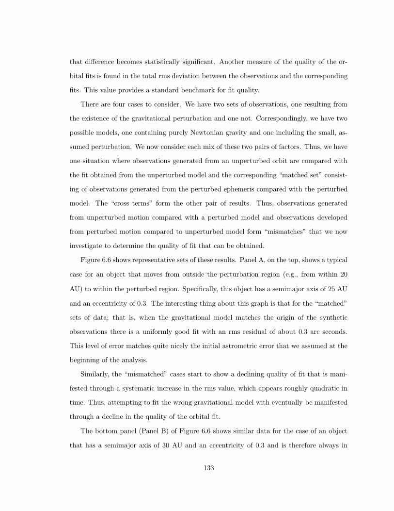
that difference becomes statistically significant. Another measure of the quality of the or-

bital fits is found in the total rms deviation between the observations and the corresponding

fits. This value provides a standard benchmark for fit quality.

There are four cases to consider. We have two sets of observations, one resulting from

the existence of the gravitational perturbation and one not. Correspondingly, we have two

possible models, one containing purely Newtonian gravity and one including the small, as-

sumed perturbation. We now consider each mix of these two pairs of factors. Thus, we have

one situation where observations generated from an unperturbed orbit are compared with

the fit obtained from the unperturbed model and the corresponding “matched set” consist-

ing of observations generated from the perturbed ephemeris compared with the perturbed

model. The “cross terms” form the other pair of results. Thus, observations generated

from unperturbed motion compared with a perturbed model and observations developed

from perturbed motion compared to unperturbed model form “mismatches” that we now

investigate to determine the quality of fit that can be obtained.

Figure 6.6 shows representative sets of these results. Panel A, on the top, shows a typical

case for an object that moves from outside the perturbation region (e.g., from within 20

AU) to within the perturbed region. Specifically, this object has a semimajor axis of 25 AU

and an eccentricity of 0.3. The interesting thing about this graph is that for the “matched”

sets of data; that is, when the gravitational model matches the origin of the synthetic

observations there is a uniformly good fit with an rms residual of about 0.3 arc seconds.

This level of error matches quite nicely the initial astrometric error that we assumed at the

beginning of the analysis.

Similarly, the “mismatched” cases start to show a declining quality of fit that is mani-

fested through a systematic increase in the rms value, which appears roughly quadratic in

time. Thus, attempting to fit the wrong gravitational model with eventually be manifested

through a decline in the quality of the orbital fit.

The bottom panel (Panel B) of Figure 6.6 shows similar data for the case of an object

that has a semimajor axis of 30 AU and an eccentricity of 0.3 and is therefore always in

133

0.0

0.2

0.4

0.6

0.8

1.0

0 20 40 60 80 100

rms

resi

dual

(ar

csec

)

Arc Length (yr)

Panel A

Ephermeris without/Gravity withoutEphermeris without/Gravity withEphermeris with/Gravity withoutEphermeris with/Gravity with

0.0

0.2

0.4

0.6

0.8

1.0

0 20 40 60 80 100

rms

resi

dual

(ar

csec

)

Arc Length (yr)

Panel B

Ephermeris without/Gravity withoutEphermeris without/Gravity withEphermeris with/Gravity withoutEphermeris with/Gravity with

Figure 6.6 Rms residual for various combinations of observations and gravity model as theobservation arc lengthens. Panel A shows the case for an object with a semimajor axis of25 AU and an eccentricity of 0.3. Panel B shows the case of an object that is always inthe perturbation region beyond 20 AU. Its semimajor axis is 30 AU and its eccentricity is0.3. Note: in the legend, “ephemeris with/without” means the synthetic observations weregenerated with/without a Pioneer perturbation; “gravity with/without” means the object’smotion is calculated with/without the additional perturbing force.

134

the assumed perturbation region. The general characteristics outlined above are found here

as well, except for a slightly slower rate of decrease in the quality of the orbital fit as time

progresses for the “mismatched” cases. The overall quality of the fit for the “matched”

cases is slightly better as well, This is probably due to this case being in an area where the

gravitational force is smoothly varying. Thus, the orbital fit does not need to accommodate

the discontinuity in acceleration present at 20 AU due to our assumed perturbation model.

The result is that while acceptable orbital fits might be obtained with “matched” ob-

servations and models, the “mismatched” cases provide inferior fits. However, it should be

noted that a sophisticated analysis of astrometric errors might be necessary to determine

that the achieved fit quality is actually inferior. All “mismatched” cases shown in Figure

6.6 still have sub-arcsecond rms residuals even after an observation arc a century long.

This buttresses the observation made at the beginning of the paper that an adjustment

of orbital parameters can conceal the existence of small perturbations; the quality of the fit

with and without the perturbation is almost indistinguishable on the basis of the degree to

which observations can match an orbital model to which they are fit for an arc of 20 years

length or more.

Figure 6.6 might be compared with Figure 3.4 in Chapter 3 and one might ask why

the rms values here are monotonically increasing while the referenced curves decrease to a

minimum before increasing and why the rate of increase in rms errors here seem so much

smaller than found previously for “mismatched” cases. There are two answers to each

of these questions. First, the earlier work dealt with an object whose orbit was already

known and which possessed a number of existing observations. Thus, new observations had

to overcome the statistical weight of the pre-existing observations and the corresponding

observation arcs. Since they were relatively few and at an uneven cadence, the rms fit was

at first improved by new observations. In the current case, the observations from the start

were evenly spaced and at a high cadence. Thus, the initial fit quality could hardly be

improved as the arc length increased.

135

Secondly, the observation cadence investigated here is much higher than that in the ear-

lier work. Thus, the statistical weight of a relatively large number of observations needed

to be overcome before the fit started to degrade significantly. Even then, the rate of degra-

dation was slower than that seen in the earlier work.

6.3 Discussion

6.3.1 Heuristic for Detection Times

The data shown in Table 6.1 represents information that can be used to obtain an heuristic

for determining our ability to observe manifestations of gravitational perturbations. By this

term we mean some rule, not necessarily physically based, that we can use to easily assess

our ability to observe such differences. Our approach to obtaining such an heuristic is to

perform a least squares fit of some simple model to a confidence limit on time to obtain

observable sky position differences.

In the analysis that follows, we will make use of a 95 percent confidence limit as a level of

significance that, practically speaking, could be construed as providing significant evidence

that a real effect is observed. Subject to the assumptions of normality discussed above, this

confidence limit is 1.965 standard deviations above the mean, assuming a two-sided test

(e.g., testing the hypothesis that the positions are different).

After some consideration, the functional form we chose for our heuristic is given by

T95 =A + Be + Ce2

an, (6.2)

where T95 is the length of time required to observe a 95 percent significant difference in

sky position, and is given in years from perihelion. A, B, C, and n are parameters to be

determined.

Again, we note that this form has no physical meaning; we are only trying to arrive at

a rule for predicting how long an observation arc is needed to distinguish between objects

136

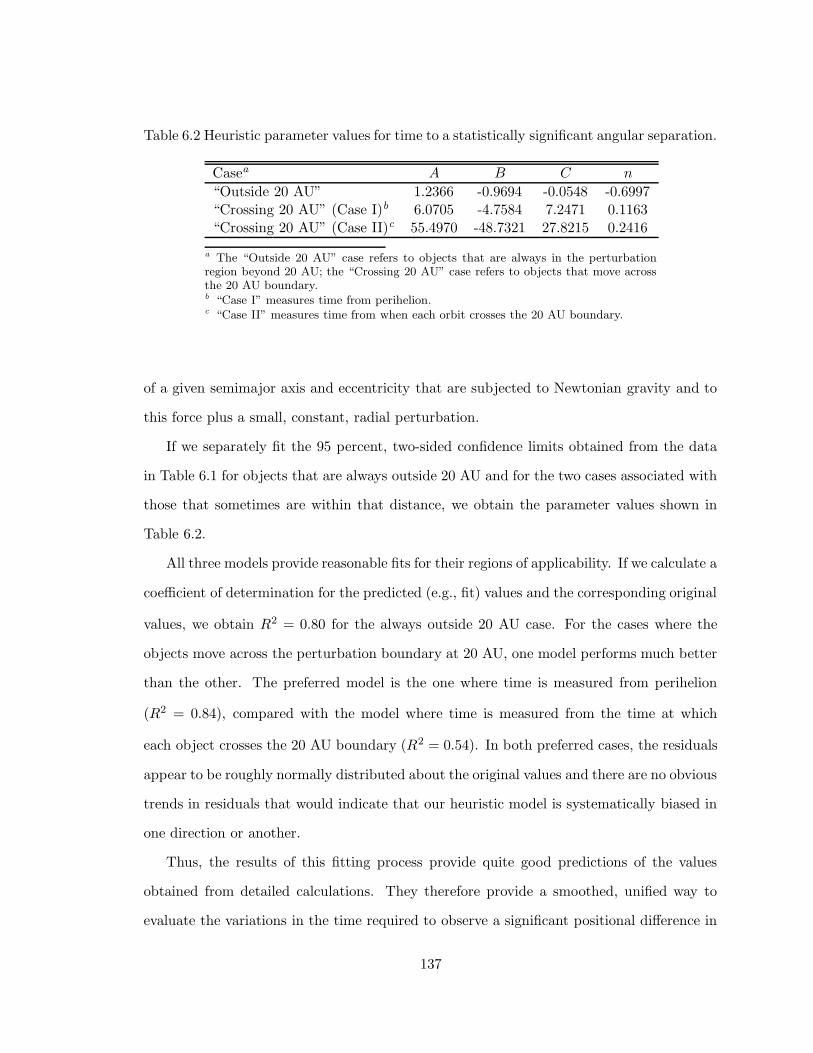
Table 6.2 Heuristic parameter values for time to a statistically significant angular separation.

Casea A B C n

“Outside 20 AU” 1.2366 -0.9694 -0.0548 -0.6997“Crossing 20 AU” (Case I)b 6.0705 -4.7584 7.2471 0.1163“Crossing 20 AU” (Case II)c 55.4970 -48.7321 27.8215 0.2416

a The “Outside 20 AU” case refers to objects that are always in the perturbationregion beyond 20 AU; the “Crossing 20 AU” case refers to objects that move acrossthe 20 AU boundary.b “Case I” measures time from perihelion.c “Case II” measures time from when each orbit crosses the 20 AU boundary.

of a given semimajor axis and eccentricity that are subjected to Newtonian gravity and to

this force plus a small, constant, radial perturbation.

If we separately fit the 95 percent, two-sided confidence limits obtained from the data

in Table 6.1 for objects that are always outside 20 AU and for the two cases associated with

those that sometimes are within that distance, we obtain the parameter values shown in

Table 6.2.

All three models provide reasonable fits for their regions of applicability. If we calculate a

coefficient of determination for the predicted (e.g., fit) values and the corresponding original

values, we obtain R2 = 0.80 for the always outside 20 AU case. For the cases where the

objects move across the perturbation boundary at 20 AU, one model performs much better

than the other. The preferred model is the one where time is measured from perihelion

(R2 = 0.84), compared with the model where time is measured from the time at which

each object crosses the 20 AU boundary (R2 = 0.54). In both preferred cases, the residuals

appear to be roughly normally distributed about the original values and there are no obvious

trends in residuals that would indicate that our heuristic model is systematically biased in

one direction or another.

Thus, the results of this fitting process provide quite good predictions of the values

obtained from detailed calculations. They therefore provide a smoothed, unified way to

evaluate the variations in the time required to observe a significant positional difference in

137

0

5

10

15

20

0 0.2 0.4 0.6 0.8 1

Tim

e F

rom

Per

ihel

ion

to 9

5% S

igni

fican

t Pos

ition

Diff

eren

ce

Eccentricity

a=45 AUa=40 AUa=35 AUa=30 AUa = 25 AU

Figure 6.7 Time (in years) from perihelion that gives a 95 percent probability of a significantdifference in sky position between a perturbed case and the unperturbed case. This graphrelates to objects that never come within 20 AU of the Sun.

the sky.

Figure 6.7 shows these smoothed results for the case where the objects in question are

always outside 20 AU. The time graphed is that from perihelion to the time that gives a

sky position difference at the 95 percent significance level. Note that the time required

with the assumed observation cadence ranges from somewhat less than ten to about 17

years, depending upon eccentricity and semimajor axis. Also note that the curves do not

terminate at their right ends. The maximum value plotted is the highest investigated that

results in the object always being in the perturbation region.

Similarly, the top panel of Figure 6.8 shows results for the case where the objects spend

some time within 20 AU and some time outside that radius. In this case, the time required to

detect a position difference at the 95 percent significance level ranges from somewhat greater

than perhaps 13 years to nearly thirty, depending upon semimajor axis and eccentricity.

The left ends of these curves do not actually terminate; rather, at smaller eccentricities,

the orbits remain outside 20 AU over their entire orbit. The plotted times are given from

138

perihelion; however, the time it takes the object to reach the 20 AU boundary can be a

significant fraction of this interval. The bottom panel of Figure 6.8 shows the same data as

the top panel, but with time measured from the time at which a given orbit crosses the 20

AU boundary.

This graph requires some explanation. In both cases, the curves are well-behaved and

essentially parallel. Note that the length of the curve corresponding to a semimajor axis

of 20 AU is the greatest. This is due to its being in the perturbed region for any value

of eccentricity. The other curves terminate at the left because smaller eccentricity values

than those corresponding to their left-handed ends will result either in their never moving

beyond 20 AU or always being outside that distance.

In both cases, the time required to obtain a statistically significant angular separation

is inversely related to semimajor axis. This is due, ceteris paribus, to the greater time spent

in the perturbation region for higher semimajor axes. However, in the case where time

is measured from perihelion, the time required to achieve a significant angular separation

generally declines with increasing eccentricity while in the case where time is measured from

the time at which each orbit crosses the 20 AU perturbation boundary, they increase. These

differences are due to geometric effects.

The greater the eccentricity, the greater the distance that must be travelled to get to

a given distance. However, the greater the eccentricity, the greater the speed at perihelion

leading to a shorter time to go a given distance. In the case where time is measured from

perihelion, the higher speed associated with a greater eccentricity more than compensates

for the greater distance to be travelled to reach the perturbation region, leading to an overall

decline in time to reach a significant position difference.

On the other hand, for the case where time is measured from crossing the 20 AU bound-

ary, a greater eccentricity implies more foreshortening of the orbital path as seen from the

Earth. This leads to a diminution of angular motion and leads to increasing times being

required to reach a significant position difference.

139

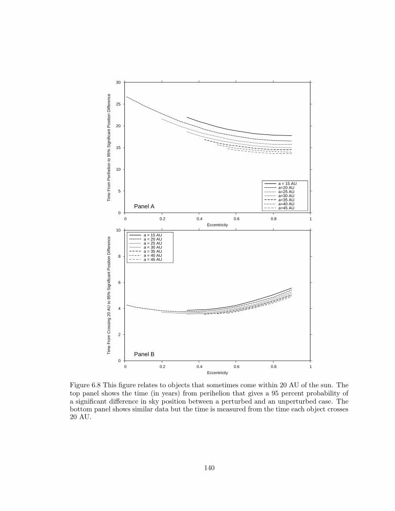
0

5

10

15

20

25

30

0 0.2 0.4 0.6 0.8 1

Tim

e F

rom

Per

ihel

ion

to 9

5% S

igni

fican

t Pos

ition

Diff

eren

ce

Eccentricity

Panel A

a = 15 AUa=20 AUa=25 AUa=30 AUa=35 AUa=40 AUa=45 AU

0

2

4

6

8

10

0 0.2 0.4 0.6 0.8 1

Tim

e F

rom

Cro

ssin

g 20

AU

to 9

5% S

igni

fican

t Pos

ition

Diff

eren

ce

Eccentricity

Panel B

a = 15 AUa = 20 AUa = 25 AUa = 30 AUa = 35 AUa = 40 AUa = 45 AU

Figure 6.8 This figure relates to objects that sometimes come within 20 AU of the sun. Thetop panel shows the time (in years) from perihelion that gives a 95 percent probability ofa significant difference in sky position between a perturbed and an unperturbed case. Thebottom panel shows similar data but the time is measured from the time each object crosses20 AU.

140

6.3.2 Physical Basis for Heuristic

These results can be presented in more physical terms by considering the angle through

which the objects move rather than the elapsed time of their motion. This alternative

geometric view helps to separate out the non-linear combinations of semimajor axis and

eccentricity that complicate interpretation of the last two figures.

Figure 6.9 shows the true anomaly at which an observable position difference between

the perturbed and unperturbed cases is found at the 95 percent significance level. As with

Figure 6.7, with which it can be compared, Figure 6.9 shows results for the case where the

objects are always outside 20 AU. The angle graphed is the true anomaly, measured from

perihelion to the position at which positional differences can be observed at the 95 percent

significance level. As alluded to earlier, this arc varies from somewhat more than 20 degrees

up to nearly 45 degrees, depending upon semimajor axis and eccentricity. Also note that,

again, the curves do not terminate at their right ends; higher values of eccentricity will not

always be within the perturbation region (e.g., at a distance of 20 AU or more).

The top panel of Figure 6.10 shows similar data for cases where the objects move between

the unperturbed and the perturbed regionand thus the objects are only in the perturbation

region part of the time. This graph shows analogous information to that shown in Figure

6.8A, but shows the true anomaly to the point on the orbit where a positional difference

can be observed at a 95 percent significance level plotted against eccentricity. The arcs

required to obtain significant position differences are very large, corresponding to the large

time intervals shown in Figure 6.8A; however, much of those arcs are occupied in moving

outwards through the unperturbed region within 20 AU.

The bottom panel in Figure 6.10 shows information analogous to that shown in Figure

6.8B, but here the arc required to observe a position difference at the 95 percent significance

level is measured from the point at which the object moves into the perturbation region.

The comments made earlier about Figure 6.8B are relevant to this figure as well.

The important point to note, however, is that it requires an observation arc ranging

from about seven degrees to 20 or more degrees beyond the entry into the perturbation

141

0

10

20

30

40

50

0 0.2 0.4 0.6 0.8 1

Tru

e A

nom

aly

at a

Tim

e to

95%

Sig

nific

ant P

ositi

on D

iffer

ence

Eccentricity

a = 25 AUa = 30 AUa = 35 AUa = 40 AUa = 45 AU

Figure 6.9 True anomaly (e.g., the angle from perihelion to the current object position alongits orbit) at which an observable position difference between the perturbed and unperturbedcases is found at the 95 percent significance level. This graph relates to objects that nevercome within 20 AU of the sun.

region to obtain unambiguous evidence (e.g., at the 95 percent significance level) of posi-

tional difference between the perturbed orbit and the unperturbed one. Recalling that the

observations of these objects begin at perihelion, this wide disparity in arcs is largely due to

the statistical weight of observations before the object enters the perturbation region. The

weight of these observations must be overcome by observations in the perturbation region

before a positional difference can be seen in the adjusted orbits.

6.3.3 What Would An Observer See?

Notwithstanding the statistical arguments made above, are there any traits that might

be seen by an observer that might lead him to think the motion of an object was not in

concordance with his model (e.g., Keplerian motion in an inverse square force)? Previously

we saw that the quality of the fit (measured by rms error), although related to the validity

of the model, did not provide unambiguous evidence one way or another. Another possible

142

0

20

40

60

80

100

120

140

160

180

0 0.2 0.4 0.6 0.8 1

Tru

e A

nom

aly

Pro

vidi

ng a

95%

Sig

nific

ant P

ositi

on D

iffer

ence

Eccentricity

Panel A


0

5

10

15

20

25

30

35

0 0.2 0.4 0.6 0.8 1

Ano

mal

y P

ast 2

0 A

U P

rovi

ding

a 9

5% S

igni

fican

t Pos

ition

Diff

eren

ce

Eccentricity

Panel B


Figure 6.10 This figure relates to objects that sometimes come within 20 AU of the sun.The top panel shows the true anomaly (e.g., the angle from perihelion to the current objectposition along its orbit) that result in observable positional differences at the 95 percentsignificance level. The bottom panel shows similar data but with the anomaly measuredfrom the anomaly at which the object moves into the perturbation region.

143

answer to this question lies in the analysis of model residuals.

The least squares procedure underlying orbital parameter fitting assumes that the er-

rors between the model and the data are normally distributed; difficulties can arise if this

assumption is violated by the data. In particular, any systematic structure to the residuals

of a model fit strongly suggests a biased model. In a series of observations, would it be

possible for the observer to unambiguously see such signs of bias? If so, this might provide

a valuable early warning of problems with his model, his data, or both.

Once again we have four cases, consisting of all combinations of observations made with–

and without a small, constant, radial gravitational perturbation in addition to Newtonian

gravity, fit to a purely Keplerian model or one containing a perturbation. As above, we can

categorize these combinations in “matching” cases and “mismatches.”

“Matched” Case

We have generated a series of synthetic observations for arcs of length eleven, 21, and 31

years, with the same thirty day observation cadence used above. This was done separately

for the perturbed and unperturbed cases, and each was separately fit to a perturbed and

unperturbed model. The residuals in each case were then inspected.

A convenient way to look for bias or trends in data like this is through graphing normal

points, which show a moving average of the stochastic data and the corresponding standard

deviation of the data over the same period. Normal points can make trends and biases more

apparent than they would be by inspecting the raw data alone.

Figure 6.11 shows such normal points for the case of an object with a semimajor axis of

25 AU and an eccentricity of 0.3. The observations are generated using unperturbed gravity

and the fitting model does not include a perturbation; thus, this is a “matched” situation

and is directly comparable to Figure 6.5A. The averaging window is one year long. Thus,

for each calendar year, the residuals of all observations made during that year are averaged

and plotted with standard deviation error bars. This type of procedure at least roughly

corresponds to averaging residuals occurring during each opposition. The topmost graph,

144

Panel A, shows the residual structure for the eleven year arc, Panel B shows the 21 year

arc, and Panel C shows the 31 year arc. The residuals shown are in right ascension, but

those for declination show a similar character.

The important point to note in this figure is that there is no discernable structure to

the residuals. Although there is a significant degree of variation within each year, the

average values are small and we certainly would not expect any of the average residuals

to be significantly different from zero. The other “matched” situation, with observations

generated with the perturbation and the fitting model including the perturbation, appears

similar.

“Unmatched” Case

Figure 6.12 shows similar data for a “mismatched” situation with observations generated

without the perturbation and the model contains the perturbation. Again, the averaging

window is one year. As above, the top panel pertains to the eleven year arc, the middle

panel to the 21 year arc, and the bottom panel to the 31 year arc. Right ascension residuals

are shown, but declination residuals are similar.

Once again, there is no discernable structure to the residuals after eleven years of obser-

vations and one could not expect the average residual to be different from zero. Although

the same statements can be made about Panel B, and one could not claim the average

residuals are significantly different from zero, there seems to be an oscillatory character to

the residuals. This trend continues in Panel C, but with the longer run of data showing

biases, it becomes clear that there might be a “mismatch” between observations and the

model. The other “mismatched” case, with observations generated with a perturbation and

the model not containing the perturbation provides similar results.

Although there is some indication that there is a trend, one cannot easily make the

argument that any of the average residuals is different from zero. Again, this confirms the

observation made earlier that a change in orbital elements can conceal the effects of a small

perturbation.

145

-1.0

-0.5

0.0

0.5

1.0

0 5 10 15 20 25 30 35

Ann

ual A

vera

ge R

A R

esid

ual (

arcs

ec)


Panel A

-1.0

-0.5

0.0

0.5

1.0

0 5 10 15 20 25 30 35

Ann

ual A

vera

ge R

A R

esid

ual (

arcs

ec)


Panel B

-1.0

-0.5

0.0

0.5

1.0

0 5 10 15 20 25 30 35

Ann

ual A

vera

ge R

A R

esid

ual (

arcs

ec)


Panel C

Figure 6.11 Normal points (see text) in right ascension for an object with a semimajor axisof 25 AU and an eccentricity of 0.3 in a “matching” case.

146

-1.0

-0.5

0.0

0.5

1.0

0 5 10 15 20 25 30 35

Ann

ual A

vera

ge R

A R

esid

ual (

arcs

ec)


Panel A

-1.0

-0.5

0.0

0.5

1.0

0 5 10 15 20 25 30 35

Ann

ual A

vera

ge R

A R

esid

ual (

arcs

ec)


Panel B

-1.0

-0.5

0.0

0.5

1.0

0 5 10 15 20 25 30 35

Ann

ual A

vera

ge R

A R

esid

ual (

arcs

ec)


Panel C

Figure 6.12 This figure shows normal points in right ascension for an object with the samesemimajor axis (25 AU) and eccentricity (0.3) as in Figure 6.11, but it is a “mismatched”case.

147

Caveats on Residual Analysis

One might therefore expect that trends or biases in residuals could provide an astute ob-

server with information indicating that there might be a “mismatch” between his model and

his observations. However, there are two important aspects of this analysis that should be

noted. First, Figures 6.11 and 6.12 both illustrate the results of a particular set of synthetic

observations. Since the observation errors are stochastic, another realization of this data

would perhaps provide a different view of potential trends and biases. Secondly, since the

data are stochastic, it is not necessarily easy to spot trends in the residuals and one would

likely be forced back into statistical arguments to determine whether discrepancies between

observations and the model are significant.

6.4 Conclusions

Before making final comments, it is desirable to reiterate the question being asked in this

analysis. In this paper, we are parametrically varying semimajor axis and eccentricity, with

these parameters treated as if their initial values are known exactly. Hence, the question

we ask in this paper is, given a known semimajor axis and eccentricity, what will happen

if we compare observations made subject to a Newtonian model of gravity with ones made

that include a small, radial, constant perturbation.

The primary purpose of this paper has been to explore the impact of high observation

cadences on our ability to use astrometry to investigate gravity in the outer Solar System.

We have seen that moderately high cadences (e.g., one observation per month) provide

a way to distinguish between Newtonian gravity and gravity perturbed by an additional

small, radial, constant acceleration. Observations beginning when the object is in the

perturbation region can detect a positional difference at the 95 percent significance level

in approximately five to eight years, depending upon orbit characteristics. Similarly, for

objects that transition between the perturbed and unperturbed regions, an observation

period of approximately ten to 30 years is required.

148

However, this lengthy period is dependent upon our assumption that the observations

began at each object’s perihelion. This implies quite a long observation arc before the

objects even enter the perturbation region. If we subtract out that initial arc inside the

20 AU boundary, the observation interval required to detect positional differences in these

transitional objects is approximately one to eight years.

The origin of this discrepancy points out the weakest part of our analysis of transitional

objects that move from within the 20 AU boundary to outside it and into the perturbation

region: we assume the observations begin at perihelion. Thus, there is a large body of

observational data inside the 20 AU boundary before objects even begin to suffer any

perturbations. The orbital element solution for such a case is heavily weighted towards the

unperturbed solution. Only when a sufficient number of perturbed observations are made

are they able to overcome the statistical weight of the unperturbed observations and begin

to change the orbit elements. This problem would be mitigated by considering observational

arcs beginning at different positions along the orbit; however, that was beyond the scope of

this paper.

As we pointed out previously, our assumed observation cadence of one observation every

thirty days and an assumed astrometric accuracy of 0.3 seconds of arc are conservative.

Pan-STARRS is expected to initially achieve a one standard deviation positional error of

200 mas, which will decrease to about 50 mas as the astrometric grid self-improves, and a

cadence of weekly or faster (Jewitt, 2003). The science goal of LSST is to obtain astrometric

accuracies of 10 mas or better at a rate of complete sky coverage every few nights (Saha

and Monet, 2005). First, we note that these astrometric accuracies are likely achievable for

relatively bright objects whose positions are measured repeatedly. For dimmer objects that

are moving, the final positional accuracy might be considerably less, perhaps 100 to 200 mas.

Although the final performance capabilities of these remarkable instruments remains to be

demonstrated, given that only a prototype Pan-STARRS instrument has seen first light

and LSST will not reach that milestone until 2012 (Sweeney, 2006), we will stand by our

assumptions as providing an accurate indicator of the initial performance of modern, high

149

cadence, automated surveys. However, we must note that eventually substantial reductions

in all the time intervals discussed in this paper are possible or even likely.

In sum, the upcoming advent of observational instruments such as Pan-STARRS and

LSST show every prospect of leading to a realistic possibility of testing the inverse square

law of gravity in the outer Solar System. These systems, with their very high observation

cadences, will completely obviate the difficulties associated with obtaining large amounts of

telescope time in which to conduct this type of observation program. Finally, an additional

factor associated with this method of assessing gravity with LSST and Pan-STARRS deals

with the use of ensembles of objects. The large number of candidate objects that should be

discovered by these instruments will provide such a large volume of data that the statistics

will be driven to determine dynamic variations associated with gravity more quickly than

possible with the single object investigated here. Together, these factors may lead to a

renascence in our ability to test the inverse square law of gravity at intermediate distance

scales.

150

Chapter 7: Astrometry Summary

As outlined in Chapter 1, the overall purpose of the dissertation is twofold. The first goal

is to investigate the use of planets, comets, and asteroids, to look at the reality of the

Pioneer effect, and in particular to determine if those bodies provide a means to evaluate

the gravitational field of the outer Solar System. The second goal is to explore two general

mechanisms for explaining the Pioneer effect within the current astrophysical context. The

latter of these goals will be addressed in Part II; the former is addressed in Part I of the

dissertation.

In particular, the goal of this part of the dissertation is to assess the feasibility of using

observations of asteroids, comets, and planets to evaluate the gravitational field in the outer

Solar System and thereby explore the Pioneer effect by means of precision astrometry. If

an independent method of measuring the Pioneer effect was available it might serve, once

and for all, to either support or refute its existence as a real phenomenon.

Specifically, this portion of the dissertation had objectives that included the following:

• Using asteroids to probe the Pioneer effect—This objective involves investigating

whether asteroids can be used to determine whether or not the Pioneer effect can

be validated by means of astrometric observations. The work shows that a sustained

observation campaign or properly chosen asteroids can over time show whether or not

the Pioneer effect exists.

• Using Pluto as a probe of gravity in the outer Solar System—Contrary to a number

of statements in the literature, and in agreement with other assertions I have made,

we show that the motion of Pluto does not indicate that the Pioneer effect does not

exist; rather, uncertainties in the orbit of Pluto conceal potential small perturbations

to gravity.

151

• Using comets to measure the Pioneer effect—This objective seeks to investigate the use

of comets to see if they provide a vehicle for measuring the Pioneer effect. As smaller

and typically fainter bodies that are also subject to nongravitational perturbations

(Marsden et al., 1973), comets are not ideal candidates for this purpose; however,

examining the general feasibility of comets in this role was the primary thrust of this

objective.

• Exploring the impact of uncoming large, high observation cadence instruments such as

Pan-STARRS and LSST on the use of objects in the outer Solar System to investigate

gravity—Recognizing the scarcity of time on large telescopes, the dissertation shows

that the advent of high speed, deep surveys will revolutionize the use of minor planets

as probes of gravity in the outer Solar System.

Each of these objectives were addressed in an individual Chapter of the dissertation and

will be summarized below.

7.1 Discussion

We showed that asteroids can fill the role of investigating whether the Pioneer effect exists.

These bodies are useful for this purpose because they have a large mass and are large and

bright enough to observe for satisfactorily long intervals. Our analysis clearly shows that

observations could determine whether or not the Pioneer effect exists, and demonstrates that

the residuals of orbital fits grow if continuing observations are conducted and are modeled

with an erroneous force model. We further demonstrate that the Pioneer effect could be

confirmed or refuted by means of a sustained observation campaign against properly chosen

asteroids. These observations can be conducted with modest allocations of telescope time,

and would provide a definitive answer to the question within the next 20 years.

As far as the outer planets are concerned, our analysis above showed two major things.

First, we must fit observations to a particular dynamical model and adjust orbital elements

152

before predicted positions on the sky can be compared. The key idea is that orbital pa-

rameters are not known. Rather, they are derived from observations which have associated

an unavoidable error. The determination of orbits is a model fitting process which has its

own associated error sources. Thus, the orbits are not known with precision in any case.

Finally, extrapolating sky positions very far past the end of an observation arc can result in

predicted observations becoming inaccurate so rapidly as to be worthless. The implication

of these findings is that “matched” and “mismatched” gravity models cannot be distin-

guished on the basis of observable sky positions for observation arc lengths similar to those

currently obtaining for the outer planets.

Similarly, in order to draw conclusions about differences in position in the sky, we must

be careful not to oversimplify the dynamical model used to draw the conclusions. Suppress-

ing degrees of freedom in the dynamics simplifies the orbital determination problem to just

such a degree. We must recognize that the orbital determination problem is nonlinear and

the customary solution methods are approximations. Thus, any missing or ignored degrees

of freedom can, if present, conceal dynamical effects associated with differing gravity models;

we are forced to make use of the full dimensionality of the dynamical problem. In particular,

a substantial amount of variation can be absorbed into a multidimensional parameter space

and the full parameter space must be considered to properly reflect differences in motion of

the outer planets due to the Pioneer effect.

Comets, although seemingly providing a potential observational vehicle for investigating

the Pioneer effect, are by no means ideal for this purpose. Although possessing many of the

qualities that made asteroids useful for this purpose, for example, because they have a large

mass and are large and bright enough to observe for possibly satisfactorily long intervals.

However, comets possess many characteristics that make them a marginal candidate

for assisting us in our quest. Generally, comets are of small size and have a low albedo.

This makes them difficult to observe at distances from the Sun where the Pioneer effect

plays a role. Also problematic is the fact that comets can be extended sources, particularly

when they are close to the Sun. Locating the center of light of a comet image can present

153

more problems than it does for asteroids. Additionally, jetting by comets produces not only

asymmetric isophotes and potentially influencing its trajectory.

Before making comments on the impact of LSST and Pan-STARRS, it is desirable to

reiterate the question being asked in this analysis. We are parametrically varying semimajor

axis and eccentricity, with these parameters treated as if their initial values are known

exactly. Hence, the question we ask in this paper is, given a known semimajor axis and

eccentricity, what will happen if we compare observations made subject to a Newtonian

model of gravity with ones made that include a small, radial, constant perturbation.

The primary purpose of this part of the dissertation has been to explore the impact

of high observation cadences on our ability to use astrometry to investigate gravity in the

outer Solar System. We have seen that moderately high cadences (e.g., one observation per

month) provide a way to distinguish between Newtonian gravity and gravity perturbed by

an additional small, radial, constant acceleration. Observations beginning when the object

is in the perturbation region can detect a positional difference at the 95 percent significance

level in approximately five to eight years, depending upon orbit characteristics. Similarly,

for objects that transition between the perturbed and unperturbed regions, an observation

period of approximately ten to 30 years is required.

7.2 Conclusions

Whether or not the type of observations investigated here allow the Pioneer effect to be

substantiated, astrometry of asteroids can be used to measure the gravitational field in the

outer Solar System. Depending upon the number and type of the measurements, it might

even be possible to break the degeneracy in the alternative predictions of different possible

explanations for the effect or differentiate between alternative gravitational theories. This

is a worthwhile program in its own right, and observations of (5338), (8405), and 1995 SN55

would be particularly helpful for this purpose.

The proposed method is not without weaknesses, however. The first weakness of our

approach is that it has less temporal resolution and lower sensitivity to perturbations than

154

would a spacecraft, dedicated or otherwise. However, the proposed observation program is

low in cost and can explore possible perturbation effects along a number of different vectors

through the Solar System, which would require multiple spacecraft. Such an observation

program could have profound effects on our understanding of the gravitational field and

implied mass distribution in the outer Solar System, and could also assist in discriminating

between alternative gravitational theories such as MOND and classical gravity, as well as

more exotic gravitational theories.

A second weakness is that our adopted model of the Pioneer effect is very simple. Since

the primary intent of this dissertation is to investigate the dynamical consequences of the

Pioneer effect, which apparently begin at large heliocentric distances, for simplicity, and

because there are no current data supporting a more gradual onset of the Pioneer effect, we

assumed the anomalous acceleration of the Pioneer effect begins abruptly at 20 AU. This

assumption, however, does not compromise the methodology. It only places limits on the

number of asteroids to consider as observational candidates. We recognize this as a simplistic

model of the effect. Alternative mechanisms exist that cause the Pioneer effect to vary with

object mass, orbital eccentricity, radial distance, and a number of other parameters of the

motion. As further observations of minor planets become available, they can potentially be

used to investigate various force models in order to explore all possibilities until either the

Effect is ruled out or its origin is found. However, the current status of information on the

Pioneer effect dictates that this simple model be investigated first.

Our analysis of Pluto’s orbit shows that we must conclude that we do not know the

orbits of the outer planets as well as we might have thought. We must continue to perform

astrometry on them in order to be able to comment on the accuracy with which we know

their orbits. In particular, we cannot assert that the motion of these bodies demonstrates

that the Pioneer effect does not exist. That jury is still out. Of course, this does not mean

that the Pioneer effect exists. It does mean that we cannot deny the existence of the Pioneer

effect on the basis of motions of the outer planets as currently known. Further observations

are required before such an assertion can be made with confidence.

155

Pluto is a particularly good target for such observations. Uranus and Neptune are

resolved objects and it is relatively difficult to determine their positions with high accuracy.

Pluto, as a much smaller object is easier to locate astrometrically. In addition, Pluto will be

visited by a spacecraft (New Horizons) in the relatively near future and should provide new

knowledge of parameters of Pluto’s orbit that can inform the kind of calculations performed

here.

We should also point out that in addition to the observations of individual objects dis-

cussed in this chapter, there are other related approaches to assessing gravity in the outer

Solar System. For example, recently Wallin et al. (2007) have investigated the use of en-

sembles of Trans-Neptunian Objects to ascertain whether their motion reflects unknown

additional perturbations. This work showed a 5-σ inconsistency between the motions ex-

hibited by these objects and the existence of the Pioneer effect. Similarly, in the area of the

observation of individual objects as discussed in this chapter, the advent of Pan-STARRS

and LSST in the next several years should provide sufficient data to determine whether the

motion of outer Solar System bodies reflect the action of unknown forces. This determi-

nation should occur over time frames discussed in this paper. However, a combination of

the techniques of Wallin et al. (2007) and the considerations presented here should provide

definitive answers more quickly.

In terms of the existence of the Pioneer effect, perhaps the most important thing comets

have to say is that if the Pioneer effect exists, the impact on the motion of comets would

not contradict the physically well-motivated NGF model. Although the NGF model pa-

rameters would have to change, the changes would result in model parameter values that

are completely reasonable.


existence or non-existence of the Pioneer effect, they do have some interesting charac-

teristics. Continuing observations such as those undertaken at the ESO (Hainaut et al.,

2004) might provide insight over time into vagaries in their motion, especially as target

comets approach aphelion. ESO observations also provided the provocative result that

156

comet 1P/Halley is approximately 1.4 seconds of arc behind its expected ephemeris posi-

tion. The idea that perturbations like the Pioneer effect could contribute to this discrepany

is worthy of further investigation.



NGF parameters are also zero. The idea of a comet with substantial outgassing flies in

the face of the physical justification for the NGF. The idea that Swift-Tuttle’s outgassing



Swift-Tuttle is a less unusual body is worthy of further investigation.

Thus, of the three classes of candidate objects, only one seems to hold promise for

ascertaining the reality of the Pioneer effect. Despite the limitations of the use of asteroids

in that role, it remains true that there are very few intermediate range tests of gravity at

the multiple AU distance scale. Comets experience reaction forces due to outgassing, and

the outer planets move very slowly and cover only some of the region of interest. Spacecraft

like Pioneer are expensive, as well as being tiny, fragile things that outgas, get pushed

about by Solar winds, and suffer reaction forces due to their radio transmissions and power

sources. Most newer spacecraft improve their guidance capabilities by conducting mid-

course corrections, leading to more motion variation and greater difficulty in discerning the

small perturbations. As was said in Chapter 3, notwithstanding all the limitations of the

proposed method, there is nothing quite as useful as a big, unwieldy, dynamically dead

chunk of rock for investigating small variations in Newton’s Laws or the mass distribution

in the outer Solar System.

The lengthy period of time estimated to be required to discern the Pioneer effect in

LSST and Pan-STARRS observations of asteroids is dependent upon our assumption that

the observations began at each object’s perihelion. This implies quite a long observation

arc before the objects even enter the perturbation region. If we subtract out that initial arc

inside the 20 AU boundary, the observation interval required to detect positional differences

157

in these transitional objects is approximately one to eight years.

The origin of this discrepancy points out the weakest part of our analysis of transitional

objects that move from within the 20 AU boundary to outside it and into the perturbation

region: we assume the observations begin at perihelion. Thus, there is a large body of

observational data inside the 20 AU boundary before objects even begin to suffer any

perturbations. The orbital element solution for such a case is heavily weighted towards the

unperturbed solution. Only when a sufficient number of perturbed observations are made

are they able to overcome the statistical weight of the unperturbed observations and begin

to change the orbit elements. This problem would be mitigated by considering observational

arcs beginning at different positions along the orbit; however, that was beyond the scope of

this work.

As we pointed out previously, our assumed observation cadence of one observation every

thirty days and an assumed astrometric accuracy of 0.3 seconds of arc are conservative.

Pan-STARRS is expected to initially achieve a one standard deviation positional error of

200 mas, which will decrease to about 50 mas as the astrometric grid self-improves, and a

cadence of weekly or faster (Jewitt, 2003). The science goal of LSST is to obtain astrometric

accuracies of 10 mas or better at a rate of complete sky coverage every few nights (Saha

and Monet, 2005). First, we note that these astrometric accuracies are likely achievable for

relatively bright objects whose positions are measured repeatedly. For dimmer objects that

are moving, the final positional accuracy might be considerably less, perhaps 100 to 200 mas.

Although the final performance capabilities of these remarkable instruments remains to be

demonstrated, given that only a prototype Pan-STARRS instrument has seen first light

and LSST will not reach that milestone until 2012 (Sweeney, 2006), we will stand by our

assumptions as providing an accurate indicator of the initial performance of modern, high

cadence, automated surveys. However, we must note that eventually substantial reductions

in all the time intervals discussed in this paper are possible or even likely.

In sum, the upcoming advent of observational instruments such as Pan-STARRS and

LSST show every prospect of leading to a realistic possibility of testing the inverse square

158

law of gravity in the outer Solar System. These systems, with their very high observation

cadences, will completely obviate the difficulties associated with obtaining large amounts of

telescope time in which to conduct this type of observation program. Finally, an additional

factor associated with this method of assessing gravity with LSST and Pan-STARRS deals

with the use of ensembles of objects. The large number of candidate objects that should be

discovered by these instruments will provide such a large volume of data that the statistics

will be driven to determine dynamic variations associated with gravity more quickly than

possible with the single object investigated here. Together, these factors may lead to a

renascence in our ability to test the inverse square law of gravity at intermediate distance

scales.

159

Part II

Dark Matter in the Solar System

160

Chapter 8: Dark Matter Methods and Models

The next two areas of discussion relate to the proposed methods of explaining the Pioneer

effect in terms of dark matter captured into Solar orbit. In both these cases, we seek to

determine the three dimensional mass density that would result from hypothesized dark

matter interactions. These density profiles can be compared with that required to generate

the Pioneer effect as well as with observed motions of all Solar System bodies. The first

method deals with a hypothetical weak interaction between elementary particle dark matter

and matter in the Sun. Existing Solar models and an isotropic dark matter distribution will

be used with a Monte Carlo simulation of the dynamics of dark matter particles to determine

the resulting phase space distribution of dark matter as a function of parameters describing

the properties of dark matter. The second mechanism is that of three body gravitational

interactions leading to capture of dark matter into Solar orbit. This mechanism involves

the Galactic barycenter, the Sun, and the dark matter particle interacting gravitationally.

Where the first method requires a weak interaction with elementary particle dark matter,

the second method would have physical validity for any form of dark matter at all.

8.1 Galactic Dark Matter Distribution

The population of dark matter that will interact with the model Sun is viewed as a relaxed,

isotropic, isothermal distribution. One example of such a model has an associated mass

161

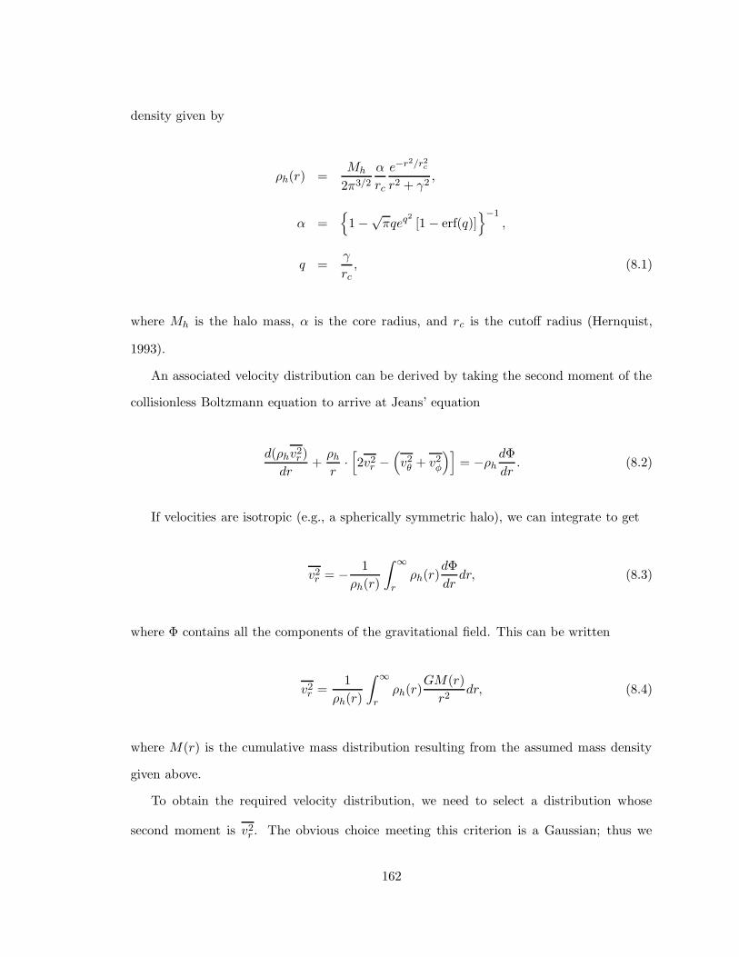
density given by

ρh(r) =Mh

2π3/2

α

rc

e−r2/r2c

r2 + γ2,

α =

1 −√

πqeq2[1 − erf(q)]

−1,

q =γ

rc, (8.1)

where Mh is the halo mass, α is the core radius, and rc is the cutoff radius (Hernquist,

1993).

An associated velocity distribution can be derived by taking the second moment of the

collisionless Boltzmann equation to arrive at Jeans’ equation

d(ρhv2r )

dr+

ρh

r·[2v2

r −(v2θ + v2

φ

)]= −ρh

dΦ

dr. (8.2)

If velocities are isotropic (e.g., a spherically symmetric halo), we can integrate to get

v2r = − 1

ρh(r)

∫∞

rρh(r)

dΦ

drdr, (8.3)

where Φ contains all the components of the gravitational field. This can be written

v2r =

1

ρh(r)

∫∞

rρh(r)

GM(r)

r2dr, (8.4)

where M(r) is the cumulative mass distribution resulting from the assumed mass density

given above.

To obtain the required velocity distribution, we need to select a distribution whose

second moment is v2r . The obvious choice meeting this criterion is a Gaussian; thus we

162

select our speeds from

f(v, r) = 4π

(1

2πv2r

)3/2

v2e−v2/2v2r , (8.5)

and we can initialize our velocity components assuming isotropy. Thus, each component is

independent and drawn from the same distribution for speed.

Now that we have justified using a Maxwell-Boltzmann distribution to describe the

velocity structure of Galactic dark matter, we must ask the question of what value for v2r

is appropriate. This question is not a simple one, notwithstanding the general acceptance

of a working value for such research. Cowsik et al. (1996) provides a description one way

to derive v2r .

The normal way to proceed is to take refuge in a virial approach and to set v2r equal

to 3/2 times the square of the asymptotic value of the Galaxy’s circular rotation speed.

The difficulty arises in that the rotation curve of the Galaxy is not known. Usually, it is

assumed that the rotation curve is flat from about 5 kpc from the center out past the Sun

at about 8.5 kpc. This gives a value of v2r

1/2of 270 km/s which is the value adopted here.

It is worth noting, however, that there are several weaknesses in this approach. First,

there is really no reason to assume a spherical distribution of Galactic dark matter (Bin-

ney and Tremaine, 1987). It could equally well be distributed in a disklike structure and

cosmological dark matter simulations show a filamentary structure. Second, Cowsik et al.

(1996) makes the provocative claim that the velocity dispersion in the Galaxy can be as

great as 600 km/s. This claim received a number of criticisms (Evans, 1997; Gates et al.,

1997), but it remains interesting. Investigation of the impact of such a large dark matter

velocity dispersion is left for future research.

163

8.2 Local Dark Matter Density

The most important observational quantity contributing to the determination of the local

density of dark matter is the Galaxy’s rotation curve. It has been measured frequenty, but

often some comment like “due to our unfortunate location within the Galaxy,” is made

to indicate the difficulty of making it accurately. One complexity is that the total mass

distribution of the Galaxy determines the rotation curve. Thus, knowledge of the disk, the

central bulge, and the halo all are necessary.

Using a variety of approaches, the local dark matter density has been calculated. The

results of these efforts are described in Jungman et al. (1996) and Bertone et al. (2005).

They relate that Bahcall et al. (1983) obtains a value of about 0.009 M/pc3, while Caldwell

and Ostriker (1981) find a smaller vale of 0.006 M/pc3. Turner (1986) found the local dark

matter density to be about 0.008-0.011 M/pc3. Others obtain results agreeing more or less

with these values. Generally, in numerical research, a value of 0.008 M/pc3 is adopted.

Since one M/pc3 = 38 GeV/cm3, this means the canonical value of the local density is

about 0.3 GeV/cm3.

This value is almost universally used in dark matter studies. However, the uncertainties

in it should be noted. As Jungman et al. (1996) points out, the “standard lore” currently

assumes an error is this value of about a factor of two. However, the uncertainties in the

measured rotation curve imply that the local density of dark matter depends strongly on

a number of aspects of the Galaxy’s structure and the associated uncertainties might be

larger than is generally assumed.

164

Chapter 9: Dark Matter Capture Via a Weak Interaction

The idea of Galactic dark matter being captured into bound Solar System orbits due to

various kinds of interactions is not new. Spergel and Press (1985), in a search for an

explanation for the then important “missing Solar neutrino” problem, investigated the

impact of a stable, neutral, massive particle in the Sun’s primordial makeup. The resulting

properties of this particle were remarkably close to the current limits set on the parameters

of dark matter. This initial work was continued in Press and Spergel (1985), to compare

the hypothesized particle properties with those known for dark matter at the time. Both

of these papers used a diffusion approach.

The following year, Gaisser et al. (1986) investigated the possibility that Galactic dark

matter would accumulate in the core of the Sun, annihilate, and produce a neutrino signal

that could be detected in deep underground detectors.

These ideas were further elaborated by Gould (1991), who looked into the idea that

gravitational diffusion of Weakly Interacting Massive Particles (WIMPs) bound to the Sun,

but crossing the orbits of the Earth, Venus, and Jupiter could lead to “indirect” capture.

Later, Gould (1992) further investigated these ideas by seeking to measure some properties

of WIMPs by comparing the strengths of the annihilation signals produced by WIMPs in

the Sun and in the Earth. This work also employed a diffusion approach.

Work in these areas continues. Damour and Krauss (1998) looked into the possibility

that perturbations due to the planets and the departure of the Solar potential from a 1/r

form allow WIMPs that are captured in the outer layers of the Sun by scattering to evolve

into orbits that no longer intersect the Sun, allowing them to persist for significant periods

of time. More recently, Lundberg and Edsjo (2004) investigated the possibility that WIMPs

can be captured by the Earth, sink to its center, annihilate, and produce a signal detectable

165

by modern neutrino telescopes.

This summary, by no means complete, has in common that a diffusive approach was

followed, either in order-of-magnitude arguments or in explicit solution to the Boltzmann

equation.

However, a different approach was recently taken in a series of papers. This approach

began (Peter and Tremaine, 2008) by noting that for any given WIMP model, the approach

taken today to evaluate the potential effectiveness of both direct and indirect dark mat-

ter detection experiments is to assume that Galactic dark matter particles dominate both

classes of phenomena. However, two processes were not included. The first was gravitational

scattering by the planets; the second was elastic scattering of dark matter in the Sun. Al-

though a diffusion approach was previously taken, the author of Peter and Tremaine (2008)

felt that a series of orbital integrations would provide additional insight. This approach has

been continued in Peter (2009a,b,c).

While interesting, this approach is focused on determining possible detection likelihoods

for dark matter candidates. We will employ a similar method to investigate whether dark

matter particles captured by the Sun by means of weak interactions can cause the Pioneer

effect. In particular, we employ what might be termed the “hot Sun” approach where the

constituents of the Sun are in thermal motion.

The remainder of this Chapter is divided into four additional sections. First, Section

9.1 discusses the methods used to accomplish the calculations used in this Chapter. Section

9.2 discusses the results of those calculations, while Section 9.3 provides discussion of them.

Finally, Section 9.4 states conclusions.


In carrying out our calculations, there are four major parts that we need to consider. First,

both in order to calculate the motion of dark matter particles through the Sun and to

determine the likelihood of scattering, as well as the speed with which target atoms are

moving, we require a detailed model of the interior of the Sun. This information also allows

166

us to calculate the gravitational potential inside the Sun. The manner in which these aspects

of our problem are addressed is dealt with in Sections 9.1.1 and 9.1.2, below.

Second, we need a model for scattering of the dark matter particles off Solar matter. For

its simplicity, we choose a simple model of isotropic hard sphere scattering; for completeness,

we will review the simple physics behind this choice in Section 9.1.3.

Third, we wish to parameterize the scattering cross section between dark matter and

Solar matter. The manner in which a cross section per nucleon is aggregated to describe

the scattering against a Solar nucleus is described in Section 9.1.4.

Finally, Section 9.1.5 describes the methodology we use to determine the likelihood of

scattering taking place and where it occurs.

9.1.1 Solar Interior Model

Since the mean free path of dark matter particles streaming through the Sun depends upon

not only the scattering cross section, but also the density of target material, and, since the

thermal velocities of Solar material likewise depend on the internal temperature of the Sun,

we require a detailed model of the Solar interior.

The model we adopt was developed for investigating neutrino fluxes emerging from the

Sun and represents one in a series of models developed for that purpose. We use the BP2000

model (Bahcall et al., 2001). Although there are more recently developed models (Bahcall

et al., 2005, for example), BP2000 is thoroughly documented and suits our requirements

admirably.

The quantities of interest in our calculations are temperature, density, mass, and mass

fraction for the constituents of interest. We included Hydrogen, Helium-4 and -3, Carbon-

12, Nitrogen-14, and Oxygen-16. Figures 9.1 through 9.4 show the main features of the

model.

167

0

0.2

0.4

0.6

0.8

1

0 0.2 0.4 0.6 0.8 1

Mas

s in

terio

r to

rad

ial d

ista

nce

(in s

olar

mas

ses)

Radius (in solar radii)

Figure 9.1 Solar mass interior to a radial distance. Distance is expressed in Solar radii andmass in Solar masses.

0

2e+06

4e+06

6e+06

8e+06

1e+07

1.2e+07

1.4e+07

1.6e+07

0 0.2 0.4 0.6 0.8 1

Tem

pera

ture

(K

elvi

n)


Figure 9.2 Solar termperature versus radial distance. Distance is expressed in Solar radii.

168

0

20

40

60

80

100

120

140

160

0 0.2 0.4 0.6 0.8 1

Den

sity

(g

/ cm

3 )


Figure 9.3 Total mass density versus radial distance Distance is expressed in Solar radii.

1e-06

1e-05

0.0001

0.001

0.01

0.1

1

0 0.2 0.4 0.6 0.8 1

Mas

s fr

actio

n by

spe

cies


HydrogenHelium-4Helium-3Carbon-12Nitrogen-14Oxygen-16

Figure 9.4 Mass fraction of main Solar constituents versus radial distance. Distance isexpressed in Solar radii.

169

9.1.2 Solar Potential

By analogy with Newton’s gravitational force law about a point mass and its associated

potential, it is easy to make the error that the Newtonian gravitational potential about

spherically symmetric mass distribution is

Φ(r) = −GM(r)

r, (9.1)

where M(r) is the mass interior to a radial distance r.1 However, it is somewhat surprising

that such an error has appeared in the refereed literature, although it has in at least one

case (Iorio, 2006).

Taking the view that the potential energy about such an extended body is the work

done in moving an object from infinity to some distance r, we can write the potential as

Φ(r) = −∫ r

∞

F (r) · dr. (9.2)

Now, if we have a body of extent R, we can write the gravitational force as

F (r) =

−GM

r2 r ≥ R

−GM(r)r2 r < R

(9.3)

where G is the Newtonian graviational constant, M is the total mass of the object, and

M(r) is the mass interior to a radius r.

1 A graduate student who shall remain nameless made this error himself as part of his oral qualifying

examination.

170

Then, for r ≥ R we have the familiar result that

Φ(r) =

∫ r

∞

GM

r2dr

= − GM

r

∣∣∣∣r

∞

= −GM

r(9.4)

For r < R, we have

Φ(r) =

∫ r

∞

GM(r)

r2dr

=

∫ R

∞

GM(r)

r2dr +

∫ r

R

GM(r)

r2dr

= − GM(r)

r

∣∣∣∣R

∞

+

∫ r

R

GM(r)

r2dr

= −GM

R

+

∫ r

R

GM(r)

r2dr (9.5)

Considering only the second term in Eq. 9.5, we can integrate by parts and get

∫ r

R

GM(r)

r2dr = − GM(r)

r

∣∣∣∣r

R

+

∫ r

R

G

r

dM(r)

drdr

= −GM(r)

r+

GM

R

+ 4π

∫ r

R

Gρ(r)

rr2dr. (9.6)

The last term arises because M(r) = 4π∫

ρ(r)r2dr which gives dM(r)/dr = 4πr2ρ(r).

171

-1e+16

-9e+15

-8e+15

-7e+15

-6e+15

-5e+15

-4e+15

-3e+15

-2e+15

-1e+15

0 0.2 0.4 0.6 0.8 1

Pot

entia

l ene

rgy

per

unit

mas

s (e

rg/g

)


Figure 9.5 Gravitational potential energy per unit mass inside the Sun. Outside the Sun,the potential takes the form Φ(r) = GM/r. Distance is expressed in Solar radii.

Substituting Eq. 9.6 into Eq. 9.5 we can write a final expression for Φ

Φ(r) = −GM(r)

r+ 4πG

∫ r

R

ρ(r)rdr. (9.7)

It is interesting to compare Eq. 9.1 with Eq. 9.7. Clearly, the second term is a correction

to the naive approach represented by Eq. 9.1.

As a final step in our calculations we can use the Solar model discussed above and can

numerically integrate the expression on the right of Eq. 9.7 to arrive at the potential inside

the Sun. Figure 9.5 shows the resulting potential.

9.1.3 Hard Sphere Scattering

For the parametric analyses being conducted here, we neither need nor desire a complicated

model of the dark matter scattering. Since it takes a particularly simple form, and since we

are in the low energy scattering regime, we elect to model isotropic hard-sphere scattering.

172

In center of mass coordinates, this type scattering takes a particularly simple form. If

vi and v′i are the velocities of the ith particle before and after scattering, respectively, and

mi is the mass of the ith particle, conservation of linear momentum and energy give

v′1 =(m1 − m2)v1 + 2m2v2

m1 + m2

v′2 =(m2 − m1)v2 + 2m1v1

m1 + m2. (9.8)

In order to carry out the scattering, the velocities of Solar nuclei are derived from

assuming that Solar constituents are in thermal equilibrium, leading us to assume that each

constituent’s speeds are distributed according to a Maxwell-Boltzmann distribution at a

local temperature from the previously discussed Solar model.

We assume that the scattering is isotropic in center of mass coordinates.

9.1.4 Scattering Cross Section

In order to simplify our calculations, we wish to parameterize the scattering cross section

between dark matter and Solar matter. A recent review (Taoso et al., 2008) addresses the

scattering of dark matter from baryonic matter. There are two possible scattering modes,

spin-dependent and spin-independent.

The cross section for spin-independent scattering is coherently enhanced compared with

the case of scattering from a single nucleon. This enhancement is approximately given by

σSIN ' A2

(µχ

µp

)2

σSIp , (9.9)

where σSIN is the total cross section between a dark matter particle and a nucleus, A is the

atomic weight of the nucleus, µχ is the reduced mass between the nucleus and the dark

matter particle, µp is the reduced mass of a proton and a dark matter particle, and σSIp is

173

the cross section between a dark matter particle and a single proton.

For spin-dependent couplings, there is no coherent enhancement, and the total cross

section is determined by unpaired nucleons in the target nucleus. For this reason, spin-

independent interactions normally dominate for scattering against heavy nuclei. The spin-

dependent cross section is proportional to A2, which obviously is much less than the spin-

independent cross section for heavy nuclei, all other things being equal.

Since our primary interest is in parameterizing the single nucleon cross section as to

investigate the effect of dark matter elastic scattering on capture of dark matter particles,

we use Eq. 9.9 to allow a one dimensional parameterization across various nuclear species

present in the Sun.

9.1.5 Scattering Depth

We use standard techniques to determine the likelihood of scattering and where it occurs.

The Solar model discussed above provides the mass density and mass fraction for each

nuclear species as a function of radial distance from the center of the Sun. The product

of these two divided by the nuclear species mass gives the number density of nuclei as a

function of position.

Then, the optical depth to scattering is given by

τ =

∫nσds, (9.10)

where n is the number density, σ is the scattering cross section against the particular nuclear

species, and ds is an element of arc length along the path over which the integration takes

place.

Then, the probability of an interaction occuring is simply

P = 1 − e−τ . (9.11)

174

Thus, in order to determine if and where an interaction occurs, we simply integrate

Eq. 9.10 along the path of the object, and calculate the probability accordingly. Standard

simulation techniques are employed to determine if a particular species interacts at a given

position along the path.

9.2 Results

The general approach we have taken to investigate dark matter scattering is straightforward.

First, we randomly determine a speed and direction for a dark matter particle. As outlined

in Chapter 8, we assume the velocity distribution of dark matter is Maxwellian with a given

vrms in a Galactocentric frame of reference. After transforming into a heliocentric frame, we

randomly generate a Solar impact parameter and determine where the dark matter particle

intersects the surface of the Sun. Using the Solar potential described above, we integrate

the dark matter particle path and determine optical depths to scattering for each nuclear

species in the Sun.

After integrating the path through the Sun, we determine which nuclear species interacts

first, where the interaction occurs, and the appropriate physical parameters at the scattering

site. Assuming the Solar material is in thermal equilibrium, we generate a target nucleus

speed by means of a Maxwell-Boltzmann distribution and an associated random direction.

Transforming into center of mass coordinates, we conduct hard sphere scattering, pick a

random outgoing direction, and transform back into heliocentric coordinates.

At this point, we can determine the escape velocity from the Sun, and determine the

destiny of the scattered dark matter particle. We accumulate appropriate statistics and

repeat the process until a specified number of dark matter interactions take place.

Figure 9.6 shows a few illustrative trajectories through the Sun. Cases I and IV are

similar and show trajectories that pass through the outer layers of the Sun. These would

not be expected to interact much because of the low densities present in those regions.

Cases II and III pass much closer to the center of the Sun, however. For a point mass, these

trajectories would be of high eccentricity and would hook sharply around the Sun before

175

-1e+11

-5e+10

0

5e+10

1e+11

-1e+11 -5e+10 0 5e+10 1e+11

SunCase ICase IICase IIICase IV

Figure 9.6 Illustrative dark matter trajectories through the Sun. Cases I, III, and IV haverelatively large impact parameters; Case II has a smaller miss distance.

leaving. However, the extended nature of our Solar model diminishes the gravitational force

in the center, leading to smaller deflections. On the other hand, the central regions of the

Sun are denser and we would expect these particles to scatter more often.

Figure 9.7 shows the resulting optical depth to scattering for two of the dark matter

trajectories. The curves relate to the Case I and Case II trajectories shown in Figure 9.6.

There are two important aspects to note. First, the optical depth is more than three orders

of magnitude greater for Case II than for Case I because the former passes through the high

density core of the Sun. Second, the time required to pass through the Sun is about twice

as great for Case II as for Case I because the latter has a greater distance through which

to pass. Of course, the increased likelihood of an interaction in the central regions of the

Sun in Case II would also involve significantly higher temperatures and the corresponding

higher target nucleus velocities.

Reviewing the discussion of scattering cross section above, we should expect the nature

of the scattering to be unchanged relative to changes in the cross section. We should

176

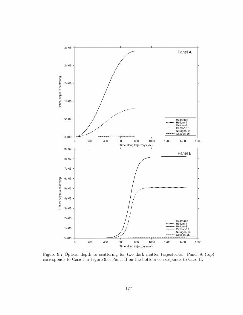
0e+00

5e-07

1e-06

2e-06

2e-06

2e-06

0 200 400 600 800 1000 1200 1400 1600

Opt

ical

dep

th to

sca

tterin

g

Time along trajectory (sec)

Panel A


0e+00

1e-03

2e-03

3e-03

4e-03

5e-03

6e-03

7e-03

8e-03

9e-03

0 200 400 600 800 1000 1200 1400 1600

Opt

ical

dep

th to

sca

tterin

g

Time along trajectory (sec)

Panel B


Figure 9.7 Optical depth to scattering for two dark matter trajectories. Panel A (top)corresponds to Case I in Figure 9.6; Panel B on the bottom corrsesponds to Case II.

177

just expect the frequency with which scattering takes place to be higher with larger cross

sections. For this reason, in the rest of this chapter we will consider only a cross section of

σ = 10−41 cm2.

For dark matter particles impacting the Sun, there are five possible outcomes. The

predominant outcome by far is that dark matter particle pass through the Sun without

interacting. For the particles that do interact, there are two possibilities. Either the particles

are captured into a bound orbit about the Sun, or they still possess enough energy after

scattering to once again escape. For those dark matter particles that are captured, some

will orbit entirely within the Sun and some will have portions of their orbits that rise above

the Solar surface.

Figure 9.8 shows the number of each of these occurrences for the five different dark

matter masses we investigated. This figure assumed a dark matter scattering cross section

of 10−41 cm2 per nucleon and was generated from 10,000 dark matter interactions.

The peak in the number of dark matter particles captured is due to a mass resonance with

Hydrogen. If we had modeled more dark matter masses separated by smaller differences,

there presumably would be a realtively sharp peak at each mass that matched one of the

constituents in our Solar model. The magnitude of the peak would be related to the amount

of that consituent present in the Sun.

The number of particles that escape the Sun after interacting is the complement of the

number captured with respect to the 10,000 interactions. Thus, we see a lessening of the

frequency of that occurrence at the mass of Hydrogen.

The numbers of particles only inside the Sun and rising above the Solar surface add to

equal the number of dark matter particles captured. Again, there is a peak around a dark

matter mass equal to that of Hydrogen. However, perhaps the most interesting feature of

this graph is the relatively constant number of particles that rise above the Sun’s surface.

This is the population of primary interest to us as it will form the group of dark matter

particles that can generate the Pioneer effect at large distances from the Sun.

Figure 9.9 shows the log of the binned frequency versus energy for the bound dark matter

178

0

1000

2000

3000

4000

5000

6000

7000

8000

9000

10000

0.1 1.0 10.0 100.0 1000.0

Fre

quen

cy

Mass of dark matter particle (proton masses)

No. capturedNo. escapingNo. outside SunNo. only inside Sun

Figure 9.8 Number of dark matter particles suffering different fates as dark matter particlemass varies. All these results are for a scattering cross section per nucleon of 10−41 cm2

and represent the results for 10,000 dark matter interactions.

particles. Somewhat unexpected is the same sort of scaling previously seen for scattering

cross section to apply to dark matter particle mass. The approximately even spacing of the

curves in Figure 9.9 show that the overall distribution of captured dark matter particles is

similar for all dark matter masses, with only the absolute frequency of occurrence varying.

For this reason, in what follows we will display only a dark matter mass of 1,000 proton

masses.

9.3 Discussion

Figure 9.10 shows the distribution in total energy of captured dark matter particles. As

discussed previously, the form of the distribution is invariant to scattering cross section and

largely invariant to dark matter particle mass. This particular case is for a cross section

per nucleon of σ = 10−41 cm2 and a mass of 1,000 proton masses.

One interesting facet of this graph is that there are no dark matter particles captured

179

1e-13

1e-12

1e-11

1e-10

1e-09

1e-08

1e-07

1e-06

1e-05

1e-04

-1e+16 -8e+15 -6e+15 -4e+15 -2e+15 0e+00

Fre

quen

cy

Total energy (erg / g)

M = 1000M = 100M = 10M = 1.0M = 0.1

Figure 9.9 Log of binned frequency of captured dark matter particles as dark matter massis varied. All these results are for a scattering cross section per nucleon of 10−41 cm2. Darkmatter masses are given in proton masses.

directly into low energy orbits near the center of the Sun. The frequency of a particular

energy increases monotonically as one moves to greater energies, maximizing at or near a

value of zero. The termination of this distribution is due, of course, to the fact that particles

of positive energy are not bound to the Sun and are thus excluded from our captured case.

The second interesting aspect of Figure 9.10 is that, since the potential energy at the

surface of the Sun is about −1.9× 1015 ergs/g, a substantial part of the energy distribution

places captured dark matter particles outside the Sun’s surface. Of course, there is a lot of

space represented by the energies between those at the Sun’s surface and infinity.

This metaphorical “lot of space” can more clearly be seen in Figure 9.11, which shows

the distribution of semimajor axes corresponding to the captured dark matter shown in

Figure 9.10. As before, the particular case shown here corresponds to a cross section per

nucleon of σ = 10−41 cm2 and a mass of 1,000 proton masses. The frequencies of other

cases scale with cross section and mass, but the form of the distribution remains the same.

Once again, we see no dark matter particles near the center of the Sun. However, the

180

0.0e+00

5.0e-06

1.0e-05

1.5e-05

2.0e-05

2.5e-05

-1e+16 -8e+15 -6e+15 -4e+15 -2e+15 0e+00

Fre

quen

cy

Total energy (erg / g)

Figure 9.10 Frequency of energy bins of captured dark matter particles. An energy corre-sponding to a particle just reaching the surface of the Sun is about 2×1015 erg/g; an energy

corresponding to reaching the Earth’s radius is about 9× 108 erg/g, indistinguishable fromzero energy in this plot. These results are for a dark matter mass of 1,000 proton massesand a scattering cross section per nucleon of 10−41 cm2. The results are illustrative of thosefor dark matter with different masses and cross sections.

peak frequency occurs inside the Sun’s surface, which is shown by the vertical dotted line

in Figure 9.11. However, from our perspective, the most important feature of this graph

is that virtually no dark matter particles have a semimajor axis more than several AU in

magnitude. Given that the eccentricities of the captured dark matter particles are high

(because they approach quite close to the Sun), these objects cannot move beyond about

twice their semimajor axis outwards. This means that virtually none of these objects move

beyond Jupiter’s orbit.

9.4 Conclusions

The major features of the orbits of captured dark matter particles have already been out-

lined. As far as the main objectives of this dissertation are concerned, Figure 9.11 tells the

tale: Virtually no dark matter is scattered into orbits that can extend out to the distances

181

0.0e+00

5.0e-06

1.0e-05

1.5e-05

2.0e-05

2.5e-05

3.0e-05

1e-04 1e-03 1e-02 1e-01 1e+00 1e+01 1e+02

Fre

quen

cy

Upper limit of distance bin (AU)

Figure 9.11 Frequency of semimajor axis for captured dark matter. These results are fora dark matter mass of 1,000 proton masses and a scattering cross section per nucleon of

10−41 cm2. The results are illustrative of those for dark matter with different masses andcross sections. The Sun’s radius is shown by the vertical dotted line.

where the Pioneer effect has been observed. Thus, we must say that this mechanism cannot

be the cause of the Pioneer effect.

In retrospect, this is understandable. If we consider the likelihood of a dark matter

particle of positive energy scattering into a different energy state, and ask what is the

likelihood that that post-scattering energy is of a magnitude sufficient to reach into the

outer Solar System, we find that likelihood to be low.

The depth of the Sun’s potential well is about 9.6×1015 ergs/g while the energy required

to reach a distance at which the Pioneer effect has been observed (e.g., 20 AU) is about

4.4×1011 erg/g. This means that if one considers a dark matter particle uniformly scattering

into a bound gravitational state in the Sun’s field, the probability of it scattering into a

state that takes it at least 20 AU outwards is the ratio of these quantities, about 5 × 10−5.

However, it must be noted that this conclusion is based on a first scattering of dark

matter by Solar material. The potential impact of multiple scatterings is left for future

182

research, although we have some preliminary results indicating that our conclusion with

respect to this mechanism being a potential cause of the Pioneer effect will not be altered.

These ideas will be discussed further below.

The energy distribution of captured dark matter shown in Figure 9.10, shows the dis-

tribution to be roughly an increasing power law in energy. Thus, the peak of the energy

distribution is approaching zero energy, an unbound state. We may safely say that, gen-

erally speaking, the captured dark matter is loosely bound to the Sun. Then, as outlined

above, we might reasonably ask what happens to the orbits of captured dark matter during

subsequent scatterings by Solar material.

The common folklore among researchers of dark matter detectors that seek annihilation

signals for dark matter in the center of the Sun is that dark matter, after capture, quickly

thermalizes and sinks to the center of the Sun. This approach is at the center of recent work

such as (Peter and Tremaine, 2008) and (Peter, 2009a,b,c), for example. This is likely true

for massive dark matter candidates such as those customarily considered. However, there

are lighter dark matter candidates such as axions and neutralinos. Particles lighter than

several times the mass of Solar constituents are likely to be scattered out of their bound

orbits on subsequent scattering by Solar material.

Figure 9.12 shows several optical depths to scattering as a function of time. The topmost

curve represents the maximal rate of increase in optical depth when motion occurs deep in

the sun at a point of maximum density. The successive lower curves show the manner in

which the optical depth to scattering increases as the particle becomes less and less tightly

bound. The “waviness” of the curves is due to their moving through regions of lower density

further from the center of the Sun. Similarly, the duration of the regions of lesser increase in

τ are longer further out from the center than when the particles are deep in higher density

regions. The bottom-most curve in Figure 9.12 illustrates the behavior for a particle whose

orbit takes it from within to well above the surface of the sun. In these latter regions, there

is no chance of an interaction and the rate of increase in τ is zero until the particle once

again enters the Sun.

183

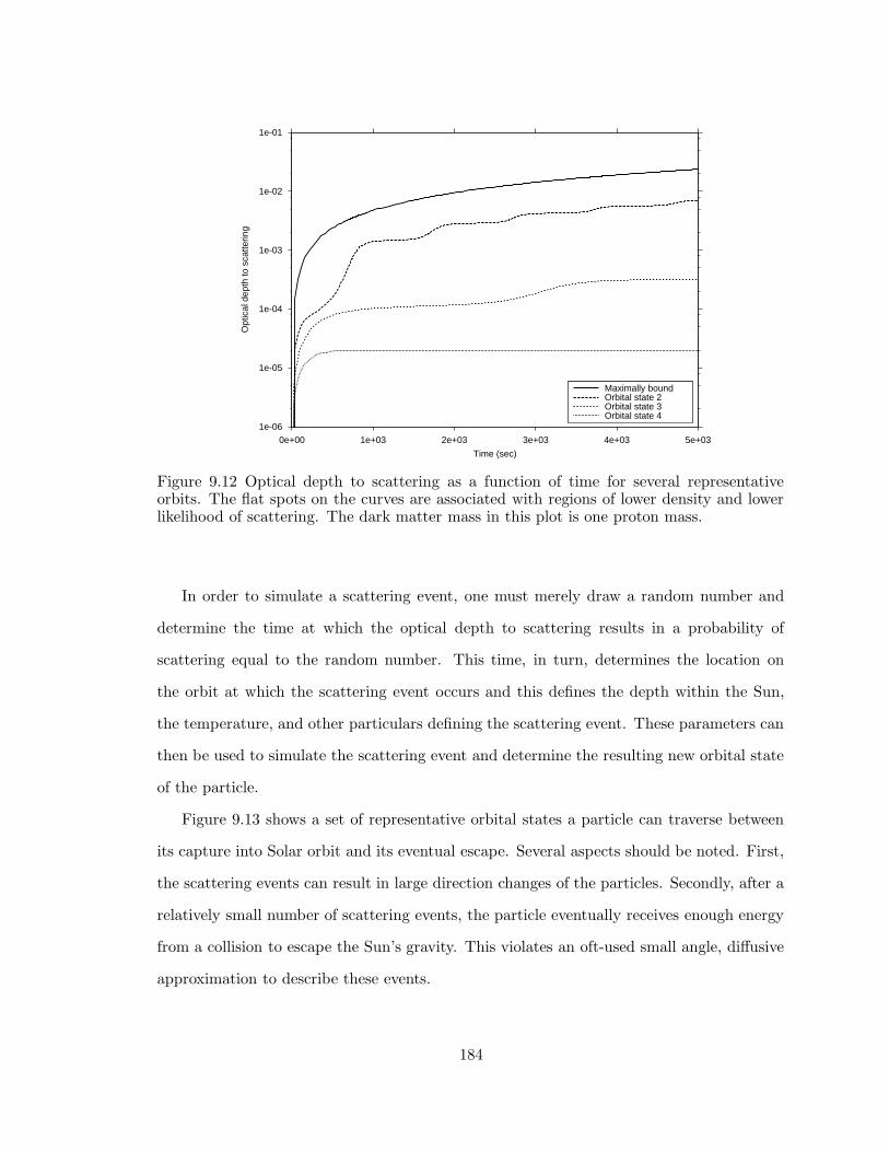
1e-06

1e-05

1e-04

1e-03

1e-02

1e-01

0e+00 1e+03 2e+03 3e+03 4e+03 5e+03

Opt

ical

dep

th to

sca

tterin

g

Time (sec)

Maximally boundOrbital state 2Orbital state 3Orbital state 4

Figure 9.12 Optical depth to scattering as a function of time for several representativeorbits. The flat spots on the curves are associated with regions of lower density and lowerlikelihood of scattering. The dark matter mass in this plot is one proton mass.

In order to simulate a scattering event, one must merely draw a random number and

determine the time at which the optical depth to scattering results in a probability of

scattering equal to the random number. This time, in turn, determines the location on

the orbit at which the scattering event occurs and this defines the depth within the Sun,

the temperature, and other particulars defining the scattering event. These parameters can

then be used to simulate the scattering event and determine the resulting new orbital state

of the particle.

Figure 9.13 shows a set of representative orbital states a particle can traverse between

its capture into Solar orbit and its eventual escape. Several aspects should be noted. First,

the scattering events can result in large direction changes of the particles. Secondly, after a

relatively small number of scattering events, the particle eventually receives enough energy

from a collision to escape the Sun’s gravity. This violates an oft-used small angle, diffusive

approximation to describe these events.

184

Figure 9.13 Representative set of orbital states that a dark matter particle traverses frominitial capture into Solar orbit to eventual escape. The encompassing circle is the Sun’ssurface. The dark matter particle mass in this plot is one proton mass.

Preliminary investigations into this capture mechanism seem to indicate that most cap-

ture orbits are of low energy and low angular momentum. The first is largely due to the

depths in the Sun’s gravitational field that particles must penetrate in order to undergo a

capture event. The second is due to the small radial distance from the center of the Sun at

which the scattering event occurs. Thus, even high energy orbits have only small angular

momentum because they necessarily intersect the Sun. Particles in orbital states such as

this will not travel very far out from the Sun.

For these reasons, it seems likely that even if we consider multiple scatterings, this

capture mode will not be a cause of the Pioneer effect because captures only place dark

matter close to the Sun, while the Pioneer effect is only observed in the outer Solar System.

However, the precision with which the positions of the inner planets are known allows one to

place bounds on the nature and phase space distribution of the dark matter in the vicinity

of the Sun. The bounds will be due to necessarily avoiding too great a mass of captured

dark matter in the inner Solar System because more captured matter would have detectable

185

consequences in terms of the motion of the inner planets.

However, these further considerations are reserved for future reseach.

186

Chapter 10: Dark Matter Capture Via Three-Body

Interactions

The idea of three body capture is familiar from its frequent use with many deep space

probes in the past. Although mostly familiar from the standpoint of allowing probes to gain

energy from planetary encounters, this mechanism has also been used to brake spacecraft

to facilitate their entry into planetary orbit. The first spacecraft to use the technique was

Mariner 10, launched in 1973. This probe used a gravity assist from a close approach

to Venus to reduce its velocity and allow a close approach to Mercury. The initial close

approach to Mercury was further used to adjust the spacecraft’s orbital period and enable

it to return to Mercury for two additional flybys.

Subsequently, the gravity assist maneuver has been used many times. Pioneer 11 was

originally planned as a Jupiter flyby, but use of Jupiter’s gravity to provide the energy for

a near reversal of direction allowed the probe to fly by Saturn only five years later on the

opposite side of the Solar System. Similarly, Voyagers 1 and 2 used a gravity assist from

Jupiter to get to Saturn and Voyager 2 used its Saturn encounter to get to Uranus and

Neptune. Ulysses used an encounter with Jupiter to radically change the plane of its orbit

and allowed it to pass over the poles of the Sun. The Galileo probe performed gravity assist

maneuvers once with Venus and twice with Earth to enable it to get to Jupiter in only six

years. Additionally, a close pass by Jupiter’s moon Io assisted Galileo in reducing its energy

and entering Jovian orbit.

As perhaps the culmination of this type of mission, the currently ongoing Cassini probe

used two flybys of Venus, the Earth, and Jupiter to get to Saturn in seven years. Once

in orbit about Saturn, multiple encounters with Titan have modified Cassinis trajectory to

allow a continuing thorough examination of the Saturnian system.

187

The physical basis of these gravity assist maneuvers is to either gain or lose energy at

the expense of a nearby object. While at first glance this seems to violate the principle of

conservation of energy, the presence of a third body enables the maneuver to be physically

realizable. Thus, for a energy-gaining flyby, the spacecraft would approach the planet from

behind, gaining energy by accelerating towards the planet. At the same time, the planet

imperceptibly slows, moving slightly closer to the Sun and into a lower energy state. This

energy difference is manifested in the increased speed of the spacecraft. A similar maneuver

passing in front of the planet can result in a loss of spacecraft energy.

In our case, the three bodies of interest are the Galactic barycenter, the Sun, and a

dark matter particle. The great depth of the Galactic gravitational potential well, the

huge mass of the Sun, and the isotropic distribution of dark matter should result in a very

large “capture basket” wherein dark matter particles can interact with the Sun and become

captured into Solar orbit. The overall geometry would seem to imply that a significant

number of the captured particles would be in high energy, high angular momentum orbits

that would extend far from the Sun. Additionally, given a lack of perturbations, these

particles, once captured, should remain in Solar orbit for a very long period of time, likely

only perturbed into escape trajectories by the infrequent close passage of other stars or

Galactic tidal effects.

The primary question that this dissertation is intended to address is whether enough

dark matter could accumulate in Solar orbit to cause the Pioneer effect.

As already discussed, even if this capture phenomenology cannot explain the Pioneer

effect, it should place constraints on the dark matter distribution in the vicinity of the Sun.

Additionally, this capture mechanism will operate with any possible type of dark matter,

whether of an elementary particle nature or not.


As is well known, the general three body problem is not soluble in closed form. From

Newton’s day, many very capable people have attempted to make headway against this

188

problem’s complexities. For our purposes here, recalling that our problem has one galac-

tically massive particle (the Galactic barycenter), one extremely massive body (the Sun),

and one almost massless body (a dark matter particle, whether micro– or macroscopic),

the circular restricted three body problem provides an excellent approach. This simplified

three body problem has been the subject of analysis for many years, and there are many

excellent treatments among which are Murray and Dermott (2000) and Valtonen and Kart-

tunen (2006), who approach the problem from different perspectives. In this discussion, we

will largely follow the treatment in Murray and Dermott (2000).

10.1.1 The Circular Restricted Three Body Problem

The circular restricted two body problem involves two massive bodies in circular orbit

about one another. The third body is comparatively massless and orbits the other two.

Importantly, the third body is so small that it has no effect on the motion of the other two

bodies at all. The two massive bodies are called the primaries and we can take their masses

to be m1 and m2. Without loss of generality, we can take m1 > m2. Then, we can define a

unit of mass such as to make G(m1 + m2) = 1 and we can write

µ =m2

m1 + m2. (10.1)

This gives the following values for the two primary masses in this set of units

µ1 = Gm1 = 1 − µ,

µ2 = Gm2 = µ, (10.2)

with µ < 1/2. The unit of length can then be chosen to make the constant separation

between the primaries unity. Similarly, we can take the unit of time to be such as to make

the period of the primaries about one another equal to 2π. This means the mean motion n

of the two primaries is unity.

189

The normal treatment of the circular restricted three body problem involves imagining

a set of rectangular inertial coordinates forming a right handed coordinate system whose

origin is at the center of mass of the two massive primaries. These coordinates can be

labeled ξ, η, and ζ and are often referred to as sidereal coordinates. We can immediately

write the equations of motion of the third body as

ξ = µ1ξ1 − ξ

r31

+ µ2ξ2 − ξ

r32

,

η = µ1η1 − η

r31

+ µ2η2 − η

r32

,

ζ = µ1ζ1 − ζ

r31

+ µ2ζ2 − ζ

r32

, (10.3)

where

r21 = (ξ1 − ξ)2 + (η1 − η)2 + (ζ1 − ζ)2,

r22 = (ξ2 − ξ)2 + (η2 − η)2 + (ζ2 − ζ)2. (10.4)

Since the two primaries are assumed to revolve around their common center of mass in

circular orbits with a constant angular velocity, their separation remains constant as well.

If we take the plane of the primary’s orbits as the ξη plane, it is then completely natural

to look at the equations of motion in a rotating frame of reference where the locations of

the primaries are fixed.

Let us then take a right handed rectangular coordinate system, with its origin also at

the center of mass of the primaries, rotating in the postive direction with a uniform rate n.

If these new coordinates are labeled x, y, and z, we can choose the x axis to lie along the line

connecting the primaries. The primaries will then have locations (x1, y1, z1) = (−µ2, 0, 0)

190

and (x2, y2, z2) = (µ1, 0, 0). Substituting into Eq. 10.4, we have

r21 = (x + µ2)

2 + y2 + z2,

r22 = (x − µ1)

2 + y2 + z2. (10.5)

In the world in which we are working, these rotating coordinates are called the synodic

coordinates.

The rotating coordinates are related to the inertial coordinates by a simple rotation

ξ

η

ζ

=

cos nt − sinnt 0

sinnt cos nt 0

0 0 1

x

y

z

. (10.6)

We can differentiate Eq. 10.6 twice to obtain

ξ

η

ζ

=

cos nt − sinnt 0

sinnt cos nt 0

0 0 1

x − 2ny − n2x

y + 2nx − n2y

z

, (10.7)

where the x and y terms have introduced the Coriolis acceleration and the x and y terms

have introduced the centripetal acceleration into the equations of motion.

We can subtitute Eqs. 10.6 and 10.7 into Eq. 10.3, and eliminate the sin and cos terms

by cross multiplying and adding and subtracting, to get the equations of motion in the

191

synodic system

x − 2ny − n2x = −[µ1

x + µ2

r31

+ µ2x − µ1

r32

],

y + 2nx − n2y = −[µ1

r31

+µ2

r32

]y,

z = −[µ1

r31

+µ2

r32

]z. (10.8)

The accelerations on the right hand side of Eqs. 10.8 plus the centripetal accelarations

can be written as the gradient of a scalar potential, U

x − 2ny =∂U

∂x,

y + 2nx =∂U

∂y,

z =∂U

∂z, (10.9)

where U is given by

U =n2

2(x2 + y2) +

µ1

r1+

µ2

r2. (10.10)

Note that U is positive, contrary to the usual convention in physics; however, this is

the norm in celestial mechanics and presents no difficulties. Note also the U is not a true

potential because its gradient does not produce all the forces on the particle in the rotating

frame.

If we multiply the three Eqs. 10.9 by x, y, and z, and add the results, we get

xx + yy + zz =∂U

∂xx +

∂U

∂xy +

∂U

∂xz. (10.11)

192

This can be integrated immediately to give

x2 + y2 + z2 = 2U − CJ , (10.12)

where CJ is a constant of integration. Rearranging terms and substituting from Eqs. 10.10,

we have

CJ = n2(x2 + y2) + 2

(µ1

r1+

µ2

r2

)− v2. (10.13)

CJ is called the Jacobi integral and it is a constant of the motion in the circular restricted

three body problem. Note that CJ is not an energy intergral because neither energy nor

angular momentum is conserved in the restricted problem. It is the only integral of motion

for this problem, however, which indicates that the problem is not soluble in the general

case.

10.1.2 Hill’s Problem

If the massless particle in the circular restricted three body problem is moving around the

larger primary, the major orbital perturbations will occur when it gets near the smaller

primary. Instead of dealing with the full equations derived above, we can simplify the

problem by describing only the motion that occurs in the vicinity of the second primary.

This problem was first developed by Hill in connection with his lunar theory (Hill, 1878).

Although many variations in this problem have been explored over the years, the starting

point we will choose for developing Hill’s problem are the equations of motion for the circular

restricted three body problem, Eqs. 10.8. Recognizing that if G is unity, the sum of µ1

and µ2 is also one, and then we can write µ1 = 1 − µ and µ2 = µ. Then, Eqs. 10.8 can be

193

written

x − 2y − x = −[(1 − µ)

x + µ

r31

+ µx − (1 − µ)

r32

],

y + 2x − y = −[1 − µ

r31

+µ

r32

]y,

z = −[1 − µ

r31

+µ

r32

]z, (10.14)

where we set n = 1 and, from Eq. 10.5,

r21 = (x + µ)2 + y2 + z2,

r22 = [x − (1 − µ)]2 + y2 + z2. (10.15)

Now, we can recognize that µ 1 which means that we can take terms like 1 − µ

and replace them with one. At the same time, we can transform from the original synodic

coordinate system centered on the center of mass of the primaries to one centered on the

less massive primary. Thus, we can substitute w = x − 1 ⇒ x = w + 1 into Eqs. 10.14 and

10.15 to get

w − 2y − (w + 1) = −[w + 1

r31

+ µw)

r32

],

y + 2w − y = −[

1

r31

+µ

r32

]y,

z = −[

1

r31

+µ

r32

]z, (10.16)

194

and

r21 = (w + 1)2 + y2 + z2,

r22 = w2 + y2 + z2. (10.17)

Finally, we recognize that w 1, which allows us to expand to first order in w, giving

r21 = 1 + 2w. Substituting into Eqs. 10.16, we get Hill’s equations

x − 2y = 3x − µ

R3x,

y + 2x = − µ

R3y,

z = −z − µ

R3z, (10.18)

where we have relabeled w as x for convenience, and

R2 = x2 + y2 + z2. (10.19)

Now, in precisely the same way as previously, we can multiply each of Eqs. 10.18 by x,

y, and z, respectively, and again obtain a perfect differential. This gives the Jacobi constant

in Hill’s approximation

CH = 3x2 − z2 +2µ

R− v2. (10.20)

As a final comment on Hill’s equations, inspection of Eq. 10.18 shows that the radial

force vanishes for µ/R3 = 3. This defines the Hill radius as

RH =(µ

3

)1/3. (10.21)

The Hill radius represents the radius within which the attractive force due to the smaller

195

primary is never less than the force due to the more massive primary. It represents a sphere

of influence about the smaller body in the presence of the larger.

10.1.3 Curves of Zero Velocity

As observed above, the Jacobi constant is the only integral of the motion available to us

in the circular restricted three body problem. This means that we cannot use it to solve

the problem in general. However, we went through the somewhat lengthy derivation of the

Jacobi constant because it can be used to determine regions from which the massless object

can be excluded.

If the velocity in the Jacobi constant is set equal to zero, we obtain a set of surfaces

that are called zero velocity surfaces. If we restrict the motion to planes, we obtain zero

velocity curves. The interesting thing about these curves is that although they are defined

by

CH = 3x2 − z2 +2µ

R, (10.22)

from Eq. 10.20, we clearly must have

CH ≤ 3x2 − z2 +2µ

R(10.23)

for the velocity to be real and not imaginary.

Since the Hill equations are derived from a set of approximations, in order to understand

how the zero velocity curves help us understand motion in the circular restricted three body

problem, we will briefly return to the full problem. In this case, the zero velocity curves are

defined by Eq. 10.13

CJ = x2 + y2 + 2

(µ1

r1+

µ2

r2

), (10.24)

where v has been set equal to zero and n to unity.

Suppose we have a body in the xy plane, very close to the more massive primary. In

196

this case, x, y, and r1 are small and r2 is about unity. Then we have a value for CJ

that is relatively large, about 2µ + 2(1 − µ)/r1. Now for v2 to be positive, we must have

CJ ≤ 2µ +2(1−µ)/r1. This can be written as r1 ≤ 2(1−µ)/(CJ − 2µ). Thus, in this case,

motion is restricted to within a small circle about the more massive primary.

Similarly, if we have a body very close to the less massive primary, x, y, and r1 are all

about unity, but r2 is small. This implies another relatively large value for CJ of about

4 − 2µ + 2µ/r2. Then, for real velocity, the motion is restricted to within a circular region

about the less massive body of radius r2 = 2µ/(CJ − 4 + 2µ).

Finally, suppose the massless body is orbiting very far away from either of the primaries.

Then, r1 and r2 are both large, and the Jacobi integral is about CJ = x2 + y2 in this initial

configuration. For the velocity to be real in subsequent motion, we must have CJ ≤ x2 +y2,

which means that the only permitted motion is outside the initial radial distance from the

center of mass of the primaries. Thus, there is a roughly circular area centered on the center

of mass within which motion is excluded.

This situation is illustrated in Figure 10.1. The important point here is that if a body

is in one of the small regions close to either of the primaries and has a Jacobi constant

with certain values, it can never escape the primary it orbits to become bound to the other

primary. Similarly, if the small object is far away from both primaries, it can have a Jacobi

constant that allows it to orbit both primaries but it can never approach either one. The

excluded area in the Figure is shaded.

In intermediate cases, there are ways for an object orbiting one primary to eventually

begin orbiting the other. Even there, depending upon specifics of the motion, the object

might never be able to leave the vicinity of the system. This is the concept of Hill’s stability

and will be discussed below.

197

Radial Distance (Hill Radii)

Tra

nsve

rse

Dis

tanc

e (H

illR

adii)

−5

−4

−3

−2

−1

0

1

2

3

4

5

−5 −4 −3 −2 −1 0 1 2 3 4 5

Figure 10.1 Zero velocity curves in the orbital plane of the primaries for µ = 0.3. The valueof the Jacobi constant is 2.5. The shaded area represents the excluded area.

10.2 Results

Our problem is a special case of the Hill problem, where the primaries are the Galactic

barycenter and the Sun. The unit of distance is about 8.5 kpc which is about 1.7 × 1020

meters. The ratio of the primary’s masses is about µ = 10−11. The Hill radius is about 1.5

× 10−4 in natural units, or about 2.6 × 1016 meters, or 0.8 pc in more familiar units. The

distance at which the Pioneer effect begins to make itself felt is 20 AU, which is about 3

× 1012 meters or about 1.8 × 10−8 in natural units. In the circular restricted three body

problem system of units, the unit of time is 1.1 × 1015 seconds, making the period of the

primaries 2π. Then, the unit of velocity is about 2.4 × 105 m/s.

We’ll look at this problem in two ways. First, suppose we have a dark matter particle at

a distance of a Hill radius divided by the square root of three away from the second primary

198

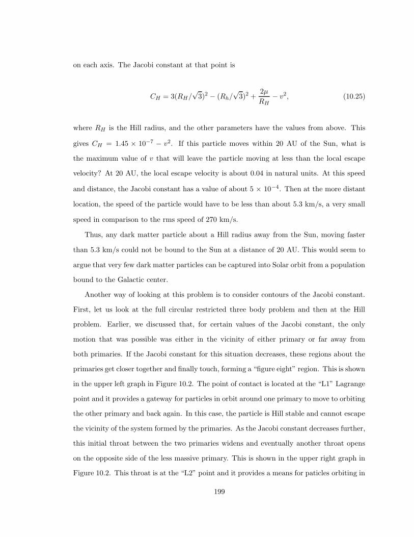
on each axis. The Jacobi constant at that point is

CH = 3(RH/√

3)2 − (Rh/√

3)2 +2µ

RH− v2, (10.25)

where RH is the Hill radius, and the other parameters have the values from above. This

gives CH = 1.45 × 10−7 − v2. If this particle moves within 20 AU of the Sun, what is

the maximum value of v that will leave the particle moving at less than the local escape

velocity? At 20 AU, the local escape velocity is about 0.04 in natural units. At this speed

and distance, the Jacobi constant has a value of about 5 × 10−4. Then at the more distant

location, the speed of the particle would have to be less than about 5.3 km/s, a very small

speed in comparison to the rms speed of 270 km/s.

Thus, any dark matter particle about a Hill radius away from the Sun, moving faster

than 5.3 km/s could not be bound to the Sun at a distance of 20 AU. This would seem to

argue that very few dark matter particles can be captured into Solar orbit from a population

bound to the Galactic center.

Another way of looking at this problem is to consider contours of the Jacobi constant.

First, let us look at the full circular restricted three body problem and then at the Hill

problem. Earlier, we discussed that, for certain values of the Jacobi constant, the only

motion that was possible was either in the vicinity of either primary or far away from

both primaries. If the Jacobi constant for this situation decreases, these regions about the

primaries get closer together and finally touch, forming a “figure eight” region. This is shown

in the upper left graph in Figure 10.2. The point of contact is located at the “L1” Lagrange

point and it provides a gateway for particles in orbit around one primary to move to orbiting

the other primary and back again. In this case, the particle is Hill stable and cannot escape

the vicinity of the system formed by the primaries. As the Jacobi constant decreases further,

this initial throat between the two primaries widens and eventually another throat opens

on the opposite side of the less massive primary. This is shown in the upper right graph in

Figure 10.2. This throat is at the “L2” point and it provides a means for paticles orbiting in

199


Tra

nsve

rse

Dis

tanc

e (H

illR

adii)

−5

−4

−3

−2

−1

0

1

2

3

4

5

−5 −4 −3 −2 −1 0 1 2 3 4 5


Tra

nsve

rse

Dis

tanc

e (H

illR

adii)

−5

−4

−3

−2

−1

0

1

2

3

4

5

−5 −4 −3 −2 −1 0 1 2 3 4 5


Tra

nsve

rse

Dis

tanc

e (H

illR

adii)

−5

−4

−3

−2

−1

0

1

2

3

4

5

−5 −4 −3 −2 −1 0 1 2 3 4 5


Tra

nsve

rse

Dis

tanc

e (H

illR

adii)

−5

−4

−3

−2

−1

0

1

2

3

4

5

−5 −4 −3 −2 −1 0 1 2 3 4 5

Figure 10.2 Zero velocity curves in the orbital plane of the primaries for different values ofCJ . The illustrated case is for µ = 0.3. Values of CJ are 1.960, 1.779, 1.646, and 1.420 forthe four cases. Equation 10.13 is defines the Jacobi constant in this problem. The shadedarea represents the excluded area.

the vicinity of the primaries to escape to the region far from them. As the Jacobi constant

decreases still further, still another throat opens on the opposite side of the more massive

primary. This is shown in the lower left panel of Figure 10.2. This throat is at the “L3” point

and provides still another entry and exit point. Finally, as the Jacobi constant decreases

still further, the throats continue to get wider and eventually the almost the entire space

is available for motion of the dark matter particles. In all these Figures, the shaded area

represents the excluded area.

In the Hill problem, the situation is similar. Figure 10.3 shows the vicinity of the less

massive primary, in the plane of the primary’s orbits, out to a distance of about two Hill

radii. The upper left panel in Figure 10.3 corresponds to Figure 10.1. Again, motion is

200

restricted to either inside the roughly circular area, or outside the two bracketing lines on

the left and the right. As the Jacobi constant is reduced, throats again open up. The

assumptions inherent in the Hill problem lead to the L1 and L2 throats opening simulta-

neously, rather than in sequence as in the full circular restricted problem. This situation

is shown in the upper right panel of Figure 10.3. Again the narrow throats allow particles,

once they have moved in close to the primary, to remain there for a period of time before

they escape. As the Jacobi constant continues to decrease, the throats continue to widen

until, as shown in the lower left panel of 10.3, there is hardly any sign of them. Finally, as

the Jacobi constant decreases further, only small excluded regions remain as shown in the

bottom right panel of 10.3. As above, the shaded areas represent the excluded areas in all

these Figures.

Physically, this means that if a dark matter particle has a Jacobi constant small enough

to be restricted to the vicinity of the primary, it can never venture away. Thus, in the

context of the Hill problem, no dark matter particles can exist outside the vicinity of the

Sun that match this criterion and that can move from outside in to the Sun’s vicinity.

However, at smaller Jacobi constant values, when the throats between the inner and outer

regions are narrow, particles entering the nearby region can remain there for an extended

period of time, moving in nonperiodic orbits in the vicinity of the Sun. However, the throats

provide egress as well as entrance and for each particle entering the region close to the Sun,

we should expect one to leave.

The wider the throats become, the more particles can flow in near the Sun, but the

easier it is for them to leave. Thus, their motion becomes more “passing near” and less

“temporarily bound” to the Sun.

The discussion above has related to the plane containing the motion of the two primaries.

Similar curves for the same values of CH used in Figure 10.3 were used to generate curves in

the plane going through both primaries and normal to the plane of the primaries’ orbits, as

well as in the plane through the lighter primary and normal to the radial direction. These

are shown in Figure 10.4.

201


Tra

nsve

rse

Dis

tanc

e (H

illR

adii)

−2

−1

0

1

2

−2 −1 0 1 2


Tra

nsve

rse

Dis

tanc

e (H

illR

adii)

−2

−1

0

1

2

−2 −1 0 1 2


Tra

nsve

rse

Dis

tanc

e (H

illR

adii)

−2

−1

0

1

2

−2 −1 0 1 2


Tra

nsve

rse

Dis

tanc

e (H

illR

adii)

−2

−1

0

1

2

−2 −1 0 1 2

Figure 10.3 Zero velocity curves for the Hill problem in the orbital plane of the primariesfor different values of CH . The values plotted are 2.5 × 10−7, 2.0 × 10−7, 1.5 × 10−7, and1.0 × 10−7. Equation 10.20 defines CH . The shaded area is the excluded area.

Radial distance

Nor

mal

dis

tanc

e

−2 −1 0 1 2

−2

−1

01

2

Transverse distance

Nor

mal

dis

tanc

e

−2 −1 0 1 2

−2

−1

01

2

Figure 10.4 Zero velocity curves for the Hill problem in the plane going through the primaryand normal to the plane of the primary’s orbits (left panel) and in the plane perpendicularto the orbital plane and normal to the radial direction (right panel). The same values forCH as were used in Figure 10.3 are used here.

202

The left panel of Figure 10.4 is similar to that shown in 10.3. Initially, the particle’s

motion will be restricted to the vicinity of the primary. As the pair of throats open, particles

can become temporarily captured, but can also escape. As the Jacobi constant diminishes

further, the throats continue to open until much of the space is available for motion of the

particle.

The right hand panel in 10.4 shows that these values of the Jacobi constant are appro-

priate for particles that are only in the vicinity of the primary. This means that particles

with these values of the Jacobi constant are not able to leave the vicinity of the primary in

the plane normal to the radial direction.

10.3 Discussion

The circular restricted three body problem is an area that is represented by a substantial

body of research going back many years. For example, Henon (1969) investigated the

restricted three body problem when the mass of the second primary was vanishingly small,

a case not dissimilar to our own. He produced families of unstable periodic orbits. However,

he did restrict himself to motion of the small body in the same plane as the primaries.

Heppenheimer and Porco (1977) also restricted themselves to plane motion, but per-

formed long term numerical integration to find orbits and illustrate their major features.

From our standpoint, their primary finding is that orbits of temporarily captured bodies

always stay at substantial distances from their primary. Heppenheimer and Porco (1977)

does show some of the peculiarities of the temporary, nonperiodic orbits, however.

Bruno and Varin (2006, 2008, 2009) represent part of a series of papers investigating

families of periodic solutions to the restricted three body problem. Many of their cases

relate to a mass ratio near zero, which matches our interests. However, they have also

restricted themselves to motion in the plane.

Almost all investigators recognize that without some form of energy dissipation, per-

manent capture in the restricted three body problem is impossible. One recent example of

such work is Vieira Neto et al. (2004) who investigated the effect of Jupiter’s mass growth

203

on satellite capture. Another such work is Iwasaki and Ohtsuki (2007) who investigated

dynamical behavior of planetesimals temporarily captured from heliocentric orbits. In their

spheres, both these works also find few temporarily captured bodies that pass close to their

primary.

Finally, Peter (2009a,b,c) consider a problem analogous to ours. We are interested in

the capture of Galactic dark matter into Solar orbit by means of three body interactions

between the Galactic barycenter, the Sun, and the dark matter particle. Peter (2009a,b,c)

investigate three body capture where the three bodies are the Sun, Jupiter, and the dark

matter particle. The thrust of these papers is towards dark matter detection through direct

detection experiments, and finding the distribution of dark matter in the Solar system in

support of that aim. They show that gravitational interactions can have an effect on such

detection rates.

In light of all this previous work and our own findings, it does not appear that three

body capture is a mechanism that can accumulate substantial quantities of dark matter

in the vicinity of the Sun and thereby produce an anomalous acceleration like the Pioneer

effect. Is does appear, however, that what capture does occur is probably restricted to

much greater distances from the Sun that is of interest to us here. However, it should be

noted that this conclusion is based upon the limitations of the circular restricted three body

problem and the derivative Hill problem. We shall say more about those restrictions below.

10.4 Conclusions

As indicated above, gravitational capture of Galactic dark matter by means of three body

interactions between the Galactic barycenter, the Sun, and dark matter particles does not

seem to be capable of producing enough captured matter to generate a Pioneer effect. What

capture does occur is temporary and would be at substantially greater distances from the

Sun than are necessary to match the characteristics of the Pioneer effect.

These conclusions, however, are based on attacking the problem with the methods of

the circular restricted three body problem and its special case, the Hill problem. The

204

underlying assumption that the small body is so small as to have no impact on the motion

of the primaries is of great import. In particular, since the primaries do not move from their

keplerian orbit about one another, neither energy nor angular momentum is conserved. As

it happens there is a conserved quantity, the Jacobi constant, but as a single integral of the

motion, it does not permit a general solution.

In the circular restricted three body problem, there is no possibility of permanent cap-

ture in the absence of some form of energy dissipation. Various mechanisms are periodically

proposed that are seemingly appropriate in particular circumstances, but external dissipa-

tion is imposed nonetheless. In the circular restricted three body problem there is no

inherent mechanism that can dissipate energy.

A simple construction due to van Allen (2003) shows that this approach may not be

adequate for all problems. Suppose we have a planet moving in an inertial frame of reference

with velocity U . Further suppose that a very small particle of initial momentum pi interacts

gravitationally with the planet. After the interaction, the small body has momentum pf =

pi +∆p. Conservation of linear momentum then requires that the momentum of the planet

change by an amount P = M(U −∆p/M) where M is the mass of the planet. The energy

of the planet after the interaction is then

P 2

2M=

1

2M[M(U − ∆p/M)]2 ,

=M

2

[U2 − 2U · ∆p

M+

∆p2

M2

]. (10.26)

Multiplying through and ignoring the very small (∆p/M)2 term, the change in energy

of the planet is

∆E =P 2

2M− M

2U2,

= −U · ∆p. (10.27)

205

Of course, if we insist that energy is conserved, the small body’s energy must change by

a corresponding amount.

The surprising thing about this result is that, at least to first order in ∆p, the amount

of energy given up by the planet is independent of the mass of either the planet or the small

particle and only depends on the geometry of the interaction and the amount of momentum

change undertaken by the small particle. This is the way that spacecraft can gain or lose

energy in planetary encounters.

However, the circular restricted three body problem does not recognize this effect. It is

doubtful that a different approach would have an impact on our conclusions with respect

to dark matter capture as a cause of the Pioneer effect. However, other applications would

make it interesting to pursue this alternative approach. This is left for future research.

206

Chapter 11: Dark Matter Summary

As was described in Chapter 1, the dissertation has two overall purposes. The first goal,

addressed in Part I, is to investigate the use of planets, comets, and asteroids to investigate

the reality of the Pioneer effect, and in particular to determine if those bodies provide a

means to evaluate the gravitational field of the outer Solar System. The second goal is to

explore two mechanisms for explaining the Pioneer effect within the current astrophysical

context. This goal is addressed in Part II of the dissertation.

Although theorists have explored many potential causes of the Pioneer effect, Occam’s

razor dictates that we preferentially investigate simpler explanations as a first choice. To

this end, the second phase of the dissertation involves exploring two general mechanisms

for explaining the Pioneer effect within the currently accepted astrophysical context.

The first approach involves investigating the effective mass density that would be pro-

duced in the Solar System as a result of the capture of elementary particle dark matter

by means of a hypothetical weak interaction between the dark matter particles and the

matter in the Sun. This approach is restricted to potential dark matter candidates such as

neutrinos or more exotic particles like neutralinos or axions that are able to interact weakly

with matter in the interior of the Sun.

The second approach to explaining the Pioneer effect involves an effect that has not

heretofore been recognized: three body capture of dark matter from the Galactic halo into

Solar orbit. We are all familiar with utilizing gravity assist trajectories to minimize travel

time for spacecraft on the way to the outer planets. What hasn’t previously been explored

is using this same dynamical phenomenon in reverse. In this case the three bodies whose

interactions can cause halo dark matter to lose sufficient energy to become bound to the

Sun are the Sun itself, the dark matter particle, and the Galactic barycenter. The process

has a very large capture cross section and has the additional benefit of applying to any

207

dark matter candidate (either elementary particle or macroscopic bodies of various levels

of exoticness).

Within the two broad purposes outlined above, the main objectives of this part of the

dissertation include the following:

• Evaluating mass capture due to particle interactions between dark matter and matter

in the Sun as a source of the Pioneer effect—If Galactic dark matter exists as ele-

mentary particles, and if it interacts both gravitationally and weakly with baryonic

matter, those interactions should lead to capture of dark matter into Solar orbit. The

thrust of this objective is to evaluate the possibility that dark matter captured in this

way can explain the Pioneer effect.

• Evaluating three-body capture as a mechanism for explaining the Pioneer effect—A

mechanism for explaining the Pioneer effect in the context of a mass concentration

in the outer Solar System that has not previously been investigated is through three-

body capture of Galactic dark matter into Solar orbit. In this context the three bodies

are the Galactic barycenter, the Sun, and the dark matter particle. Note that this

mechanism does not demand that dark matter be of an elementary particle nature.

Any type of dark matter that gravitates would be subject to this effect.

Each of these objectives were addressed in an individual Chapter of the dissertation and

will be summarized below.

11.1 Discussion

Independent of the amount of dark matter captured into Solar orbit by means of a weak

interaction with Solar matter, we have found that the nature of the orbits is such that they

cannot contribute to causing a Pioneer style acceleration at large distances from the Sun.

Virtually no dark matter is scattered into orbits that can extend out to the distances where

the Pioneer effect has been observed. Thus, we must say that this mechanism cannot be

the cause of the Pioneer effect.

208

If we consider the likelihood of a dark matter particle of positive energy scattering into

a different energy state, and ask what is the likelihood that that post-scattering energy is

of a magnitude sufficient to reach into the outer Solar System, we find that likelihood to

be low. This can be seen because the depth of the Sun’s potential well is about 9.6 × 1015

ergs/g while the energy required to reach a distance at which the Pioneer effect has been

observed (e.g., 20 AU) is about 4.4×1011 erg/g. Thus, if one considers a dark matter particle

uniformly scattering into a bound gravitational state in the Sun’s field, the probability of it

scattering into a state that takes it at least 20 AU outwards is the ratio of these quantities,

about 5 × 10−5.

However, it must be noted that this conclusion is based on a first scattering of dark

matter by Solar material. The potential impact of multiple scatterings is left for future

research, although we have some preliminary results indicating that our conclusion with

respect to this mechanism being a potential cause of the Pioneer effect will not be altered.

These ideas will be discussed further below.

The energy distribution of captured dark matter is roughly an increasing power law in

energy. Thus, the peak of the energy distribution is approaching zero energy, an unbound

state. Generally speaking, the captured dark matter is loosely bound to the Sun. Then, as

outlined above, we might reasonably ask what happens to the orbits of captured dark matter

during subsequent scatterings by Solar material. These questions are discussed below.

Gravitational capture of Galactic dark matter by means of three body interactions

between the Galactic barycenter, the Sun, and dark matter particles does not seem to be

capable of producing enough captured matter to generate a Pioneer effect. What capture

does occur is temporary and would be at substantially greater distances from the Sun than

are necessary to match the characteristics of the Pioneer effect.

It is possible that other approaches to the dynamics of this problem may result if further

insight. These approaches are left to future research. However, some comments will be made

below.

209

11.2 Conclusions

The common folklore among researchers of dark matter detectors that seek annihilation

signals for dark matter in the center of the Sun is that dark matter, after capture, quickly

thermalizes and sinks to the center of the Sun. This is likely true for massive dark matter

candidates such as those customarily considered. However, there are lighter dark matter

candidates such as axions and neutralinos (for example, Bottino et al., 2005; Lin et al.,

2009). Particles lighter than several times the mass of Solar constituents are likely to be

scattered out of their bound orbits on subsequent scattering by Solar material.

Our preliminary investigations into this capture mechanism seem to indicate that most

capture orbits are of low energy and low angular momentum. The first is largely due to the

depths in the Sun’s gravitational field that particles must penetrate in order to undergo a

capture event. The second is due to the small radial distance from the center of the Sun at

which the scattering event occurs. Thus, even high energy orbits have only small angular

momentum because they necessarily intersect the Sun. Particles in orbital states such as

this will not travel very far out from the Sun.

For these reasons, it seems likely that even if we consider multiple scatterings, this

capture mode will not be a cause of the Pioneer effect because captures only place dark

matter relatively close to the Sun, while the Pioneer effect is only observed in the outer

Solar System. However, the precision with which the positions of the inner planets are

known allows one to place bounds on the nature and phase space distribution of the dark

matter in the vicinity of the Sun. The bounds will be due to necessarily avoiding too great

a mass of captured dark matter in the inner Solar System because more captured matter

would have detectable consequences in terms of the motion of the inner planets.

However, investigating the issues associated with multiple scatterings may have signif-

icant implications with regard to the appropriateness of the customary assumptions about

the rate at which interacting dark matter comes into thermal equilibrium with Solar mat-

ter. This, in turn, has implications regarding the effectiveness of some direct dark matter

detection methods.

210

Multiple scattering effects might also conflict with the assumptions associated with dif-

fusive approximations to the outcomes of such encounters. Our preliminary results indicate

that not only are large angle scatterings the norm in our situation, but only a few encounters

are necessary to permit the dark matter particle to escape the Sun’s influence forever.

As observed above, we found that there is no possibility of permanent capture via the

circular restricted three body problem in the absence of some form of energy dissipation.

Various mechanisms are periodically proposed that are seemingly appropriate in particular

circumstances, but external dissipation is imposed nonetheless. In the circular restricted

three body problem there is no inherent mechanism that can dissipate energy.

Thus, we cannot have permanent capture of gravitationally interacting dark matter. It

also appears that dark matter particles captured by this mechanism would generally be

found too far from the Sun to generate the Pioneer anomaly. Further, we found that the

amount of dark matter likely to be temporarily captured is too small to cause the Pioneer

effect

These conclusions, however, are based on attacking the problem with the methods of

the circular restricted three body problem and its special case, the Hill problem. The

underlying assumption that the small body is so small as to have no impact on the motion

of the primaries is of great import. In particular, since the primaries do not move from their

Keplerian orbit about one another, neither energy nor angular momentum is conserved. As


motion, it does not permit a general solution.

211

Part III

Discussion and Conclusions

212

Chapter 12: Conclusions and Final Comments

12.1 Conclusions

12.1.1 Astrometry

Our conclusions fall into two areas. First, they deal with using astrometry to deterimine

whether the Pioneer effect, or any other small perturbation to gravity, exists in the outer

Solar System. Second, our conclusions deal with two potential causes to the Pioneer effect

that involve capture of Galactic dark matter into the Solar System. In the paragraphs that

follow, we will summarize the conclusions of the dissertation.

We show that asteroids can be used to evaluate the gravitational field in the outer Solar

System and can be used to explore the Pioneer effect by means of precision astrometry.

Asteroids are useful for this purpose because they have a large mass and are large and

bright enough to observe for satisfactorily long intervals. Our analysis clearly shows that

observations could determine whether or not the Pioneer effect exists, and demonstrates that

the residuals of orbital fits grow if continuing observations are conducted and are modeled

with an erroneous force model. We further demonstrate that the Pioneer effect could be

confirmed or refuted by means of a sustained observation campaign against properly chosen

asteroids. These observations can be conducted with modest allocations of telescope time,

and would provide a definitive answer to the question within the next 20 years.

However, it should be noted that Wallin et al. (2007), using ensembles of Trans-Neptunian

Objects, showed that the existence of the Pioneer effect is inconsistent with the motion of

these bodies at the 5-σ level. Similarly, Standish (2008) showed that the motion of Uranus

and Neptune is also inconsistent with the Pioneer effect.

In assessing the utility of using astrometry of the outer planets to determine whether

the Pioneer effect exists, our analysis showed two major things. First, observations must be

213

fit to a particular dynamical model and orbital elements must be adjusted before predicted

positions on the sky can be compared. Orbital parameters are derived from observations

which have associated an unavoidable error. The determination of orbits is a model fitting

process which has its own associated error sources. Extrapolating sky positions very far

past the end of an observation arc can result in predicted observations becoming inaccurate

so rapidly as to be worthless. The implication of these findings is that “matched” and “mis-

matched” gravity models cannot be distinguished on the basis of observable sky positions

for observation arc lengths similar to those currently available for Pluto.

Similarly, in order to draw conclusions about differences in position in the sky, we

must be careful not to oversimplify the dynamical model used to draw the conclusions.

Suppressing degrees of freedom in the dynamics simplifies the orbital determination problem

to just such a degree. The orbital determination problem is nonlinear and the customary

solution methods are approximations. Thus, any missing or ignored degrees of freedom can,

if present, conceal dynamical effects associated with differing gravity models; we are forced

to make use of the full dimensionality of the dynamical problem. In particular, a substantial

amount of variation can be absorbed into a multidimensional parameter space and the full

parameter space must be considered to properly reflect differences in motion of the outer

planets due to the Pioneer effect.

The problem with a simplified dynamical approach is a two-faceted one. First, the orbital

fitting problem is inherently nonlinear and is normally solved in the linear approximation.

Even if not mathematically chaotic, the system of equations is sensitively dependent upon

initial conditions. Thus, small changes in elements can result in large changes in predicted

position outside the range of observations. This sensitivity is exacerbated by the problem

of a short observation arc. The length of the entire observational archive for Pluto is

less than about one-third of a complete revolution. Together, these factors conspire to

potentially generate large errors outside the observation arc, while increasing the length of

the observation arc can markedly reduce error over the whole of the arc and even beyond

it.

214

We conclude that we do not know the orbit of Pluto as well as we might have thought.

We must continue to perform astrometry on it in order to be able to comment on the

accuracy with which we know its orbit. Using current data, we cannot assert that the

motion of Pluto demonstrates that the Pioneer effect does not exist. That jury is still out.

Of course, this does not mean that the Pioneer effect exists. It does mean that we cannot

deny the existence of the Pioneer effect on the basis of motions of Pluto as currently known.

Further observations are required before such an assertion can be made with confidence.

We showed that comets, although seemingly providing a potential observational vehicle

for investigating the Pioneer effect, are by no means ideal for this purpose. Although

possessing many of the qualities that made asteroids useful, for example, because they have

a large mass and are large and bright enough to observe for possibly satisfactorily long

intervals.

However, comets possess many characteristics that make them marginal candidates for

this purpose. Generally, comets are of small size and have a low albedo. They are bright

only when they are close to the Sun and non-gravitational forces (NGF) come into play

in this regime. This makes comets difficult to observe at distances from the Sun where

the Pioneer effect plays a role. Also problematic is the fact that comets can be extended

sources. Locating the center of light of a comet image can present more problems than

presented by asteroids.

It is interestng to note that the impact of the Pioneer effect on the motion of comets is of

the same order as that rectified by NGF–several days difference in orbital period. In terms

of the existence of the Pioneer effect, perhaps the most important thing comets have to say

is that if the Pioneer effect exists, the impact on the motion of comets would not contradict

the physically well-motivated NGF model. Although the NGF model parameters would

have to change, the changes would result in model parameter values that are completely

reasonable.


215

existence or non-existence of the Pioneer effect, they do have some interesting character-

istics. An analysis of distant observations might provide insight over time into variations

in their motion, especially as target comets approach aphelion. ESO observations also pro-

vided the provocative result that comet 1P/Halley is approximately 1.4 seconds of arc from

its expected ephemeris position at the time of the observations. The idea that perturbations

like the Pioneer effect could contribute to this discrepany is worthy of further investigation.



NGF parameters are also zero. The idea of a large comet with substantial outgassing flies

in the face of the physical justification for the NGF. The idea that Swift-Tuttle’s outgassing



Swift-Tuttle is a less unusual body is worthy of further research.

Finally, we explored the impact of high observation cadences on our ability to use astrom-

etry to investigate gravity in the outer Solar System. We determined that moderately high

cadences (e.g., one observation per month) provide a way to distinguish between Newtonian

gravity and gravity perturbed by an additional small, radial, constant acceleration such as

the Pioneer anomaly. Observations beginning when the object is in the perturbation region

can detect a positional difference at the 95 percent confidence level in approximately five

to eight years, depending upon orbit characteristics. Similarly, for objects that transition

between the perturbed and unperturbed regions, an observation period of approximately

ten to 30 years is required.

However, this lengthy period is dependent upon our assumption that the observations

began at each object’s perihelion. This implies quite a long observation arc before the

objects even enter the perturbation region. If we subtract out that initial arc inside the

20 AU boundary, the observation interval required to detect positional differences in these

transitional objects is approximately one to eight years.

The upcoming advent of observational instruments such as Pan-STARRS and LSST

216

show every prospect of leading to a realistic possibility of testing the inverse square law

of gravity in the outer Solar System. These observation systems, with their very high

observation cadences, will completely obviate the difficulties associated with obtaining large

amounts of telescope time in which to conduct this type of observation program. Finally,

an additional factor associated with this method of assessing gravity with LSST and Pan-

STARRS deals with the use of ensembles of objects. The large number of candidate objects

that should be discovered by these instruments will provide such a volume of data that

the statistics will be driven to determine dynamic variations associated with gravity more

quickly than possible with the single object investigated here. Together, these factors may

lead to a significant enhancement in our ability to test the inverse square law of gravity at

intermediate distance scales.

12.1.2 Dark Matter Capture

In considering the capture of Galactic dark matter into Solar orbit by means of a weak

interaction with Solar matter, we investigated the major features of the orbits of captured

dark matter particles. As far as the main objectives of this dissertation were concerned,

virtually no dark matter is scattered into orbits that can extend out to the distances where

the Pioneer effect has been observed. Thus, we must say that this mechanism cannot be

the cause of the Pioneer effect.

In retrospect, this is understandable. If we consider the likelihood of a dark matter

particle of positive energy scattering into a different energy state, and ask what is the

likelihood that that post-scattering energy is of a magnitude sufficient to reach into the

outer Solar System, we find that likelihood to be low.

The impact of multiple scattering is unknown at present. However, preliminary infor-

mation suggests that many captured dark matter particles will be expelled from the Solar

System in subsequent scatterings. It would remain unlikely, though, that these subsequent

scatterings would put dark matter far enough from the Sun to contribute to the Pioneer

effect.

217

Gravitational capture of Galactic dark matter by means of three body interactions

between the Galactic barycenter, the Sun, and dark matter particles does not seem to be

capable of producing enough captured matter to generate a Pioneer effect. What capture

does occur is temporary and would be at substantially greater distances from the Sun than

is necessary to match the characteristics of the Pioneer effect.

This conclusion, however, is based on attacking the problem with the methods of the

circular restricted three body problem and its special case, the Hill problem. The underlying

assumption that the small body is so small as to have no impact on the motion of the

primaries is of great import. In particular, since the primaries do not move from their

keplerian orbit about one another, neither energy nor angular momentum is conserved. As


motion, it does not provide enough information to produce a general solution.

There is no possibility of permanent capture via the circular restricted three body prob-

lem in the absence of some form of energy dissipation. Various mechanisms are periodically

proposed that are seemingly appropriate in particular circumstances, but external dissi-

pation is imposed nonetheless. In the circular restricted three body problem there is no

inherent mechanism that can dissipate energy.

However, a close look at the dynamics of the three body interaction might provide a

means for energy dissipation. This is a matter for future research.

12.2 Impact of Dissertation

The dissertation deals with a number of fundamental astrophysical questions and issues

that illustrate the importance of the overall problem area addressed:

• Does Newtonian gravity really operate at intermediate scales?

• Does dark matter really exist?

• If so, what are the parameters describing its distribution in the Galaxy?

218

• Why does there seem to be no Pioneer-like effect in the inner Solar System?

• Are there differences in the dynamics of bound and unbound orbits?

Although not directly addressing all these issues, the work accomplished in this disser-

tation should have a significant impact because of its application of new approaches to the

problems of determining whether the Pioneer effect exists and whether dark matter can be

a cause. Independent of the fact that dark matter does not appear capable of causing the

Pioneer effect, minor planets can provide an alternative approach to determining the reality

of the Pioneer effect. At this writing, we have published three papers on these matters that

directly come from the dissertation research, and another that represents a related concept.

More papers are expected.

In particular, we have accomplished the following:

• We have explored the feasibility of using asteroids to determine if Pioneer effect exists.

This work has been published in The Astrophysical Journal (Page et al., 2006). It

was also presented orally to the 207th meeting of the AAS (Page et al., 2005).

• We have investigated whether the outer planets could be used in a similar fashion.

This work has been accepted by The Astrphysical Journal and is scheduled to appear

in the 1 June 2009 issue (volume 697).

• We have evaluated the feasibility of using comets to determine the existence of the

Pioneer effect.

• We have looked at the likely impact of LSST and Pan-STARRS in terms of providing

a large database for investigating gravity in the outer Solar System.

• We have determined that capture of dark matter into Solar orbit by means of a weak

interaction with Solar matter is not a feasible cause of the Pioneer effect.

• We have found that capture of dark matter into Solar orbit by means of three body

interactions bewteen the Galactic barycenter, the Sun, and the dark matter particle

cannot cause the Pioneer effect.

219

Methodologically, the approach utilized here is new because virtually all investigators

of gravity are either operating at very small (e.g., laboratory) or very large (e.g., galactic

or galaxy cluster) scales. Although the Pioneer effect is often viewed as being a potential

test of gravity at intermediate scales, the use of minor planets and other similar bodies had

not heretofore been explored.

Generally speaking, theorists considering gravity at these scales are operating in an

empirical vacuum. The approach proposed here offers a vehicle for obtaining some useful

observational data in an alternative way and in a shorter time frame than required for

spacecraft, dedicated or otherwise.

The overall thrust of the dissertation, coupled with this initial application area of study-

ing the possibility that dark matter is the cause of the Pioneer effect is of great current

interest. If for no other reason than this current interest, studying the consequences of such

ideas provided an excellent motivation for the work.

The idea of searching for observational evidence for and consequences of dark matter at

Solar System scales is interesting because dark matter is often assumed to exist without a

lot of criticism of its problems as a concept. Observationally and theoretically, gravity in

the Solar System remains one of the more significant in astronomy and astrophysics, tied

as it is to the intersection of our knowledge of gravity at laboratory and Galactic scales.

The dissertation offers an opportunity to find out more about the empirical reality of dark

matter in the Galaxy.

12.3 Future Research Areas

This dissertation shows that the goal of using astrometry to investigate gravity in the outer

Solar System is one that could profitably be explored.

Interestingly, the relatively near-term commencement of operations of the LSST and

Pan-STARRS will further this end by likely discovering many additional candidates for

observation. The whole idea of conducting observations of minor planets at large distances

from the Sun is one that is generally not pursued. Typically, unless there is a chance of

220

an Earth impact, once enough observations of an object are obtained to reasonably well

characterize its orbit, further observations are not conducted. Thus, the suggestion that

the orbits be followed at larger heliocentric radii is one that represents a new opportunity

and justification for observing these objects.

Further observations of outer Solar System objects, and the analysis of that data should

undergo a renaissance with the advent of LSST and Pan-STARRS. The wealth of data

produced by these instruments will provide the capability of applying statistical techniques

to the approach taken here. A meta-analysis of observations of multiple objects could bear

significant fruit.

The orbits of many asteroids whose observation arcs are currently very short will be

improved immensely as well.

Further analysis of existing comet observations might also be interesting. Two major

candidates are 1P/Halley and 109P/Swift-Tuttle. The former has observations now going

out to 28 AU and shows an enticing discrepancy between its measured and predicted loca-

tions. The latter is unique in that its NGF parameters are zero, which seems at variance

to its brightness and assumed size. Investigation of the possibility that the Pioneer effect

impacts its orbit would be of great interest.

Additionally, even though attempting to explain the Pioneer effect through the capture

of dark matter into Solar orbit is not feasible, issues associated with that analysis point the

way to two areas of future research.

First, the impact of multiple scatterings between dark matter and Solar nuclei would

have great interest. The possibility that these multiply scattered objects could not con-

tribute to causing the Pioneer effect should not be discounted, but the impact of multiple

scatterings on the density of captured dark matter in the Sun is of great interest to people

concerned with the design and conduct of direct dark matter detection experiments.

Secondly, the idea that approaches other than that of the circular restricted three body

problem might provide additional insight into three body capture is provocative. There

are a number of areas where such an analysis might be significant. Some of these include

221

planetary accretion, the acquisition of irregular satellites by planets, the “fly-by anomaly,”

and others.

All these areas seem fruitful to pursue in the future.

12.4 Final Remarks

The importance of this work is seen in the continued strong interest in the Pioneer effect

and its underlying causes. Even if the Pioneer effect can be shown to be due to one or more

of the multitude of systematic effects that are currently not well understood, the likely

outcome of such a finding would be recognition that greater care is needed in characterizing

spacecraft destined for high precision missions. Thus, this endeavor would be worthwhile

to engineers and others on its own merits.

However, if the Pioneer effect were shown to exist, at the very least it would lead to

greater interest in understanding the mass density in the outer Solar System. Potentially,

it could lead to the opening of entirely new vistas in gravity theory. These possibilities,

however unlikely, are the engine driving current interest in the Pioneer effect. In this

dissertation, I discuss a new vehicle for obtaining observational information on the Pioneer

effect that can guide theorists now and provide a complimentary view of the phenomenon

as space-based measurements take place in the future. This process fosters the important

empirical end that we continue to explore all possibilities until either the Pioneer effect is

ruled out or its origin is found.

Thus, this dissertation addressed important issues in astronomy and astrophysics, was

observationally well founded, has uncovered new and unique aspects of the natural world,

and has already resulted in a number of papers that have been cited repeatedly. Finally,

the work accomplished in the dissertation has pointed the way to further research areas,

surely a mark of a successful endeavor.

finis

222

Bibliography

223

Bibliography

Anderson, J. D., Laing, P. A., Lau, E. L., Liu, A. S., Nieto, M. M., and Turyshev, S. G., 1998,Indication, from Pioneer 10/11, Galileo, and Ulysses Data, of an Apparent Anomalous,Weak, Long-Range Acceleration, Physical Review Letters 81, 2858–2861.

Anderson, J. D., Laing, P. A., Lau, E. L., Liu, A. S., Nieto, M. M., and Turyshev, S. G.,1999a, Anderson et al. Reply:, Physical Review Letters 83, 1893–+.

Anderson, J. D., Laing, P. A., Lau, E. L., Liu, A. S., Nieto, M. M., and Turyshev, S. G.,1999b, Anderson et al. Reply:, Physical Review Letters 83, 1891–+.

Anderson, J. D., Laing, P. A., Lau, E. L., Liu, A. S., Nieto, M. M., and Turyshev,S. G., 2002a, Study of the anomalous acceleration of Pioneer 10 and 11, Phys. Rev. D65(8), 082004–+.

Anderson, J. D., Lau, E. L., Krisher, T. P., Dicus, D. A., Rosenbaum, D. C., and Teplitz,V. L., 1995, Improved Bounds on Nonluminous Matter in Solar Orbit, ApJ 448, 885–+.

Anderson, J. D., Lau, E. L., Taylor, A. H., Dicus, D. A., Teplitz, D. C., and Teplitz, V. L.,1989, Bounds on dark matter in solar orbit, ApJ 342, 539–544.

Anderson, J. D., Lau, E. L., Turyshev, S. G., Laing, P. A., and Nieto, M. M., 2001, Search fora Standard Explanation of the Pioneer Anomaly, ArXiv General Relativity and QuantumCosmology e-prints, gr-qc/0107022.

Anderson, J. D., Turyshev, S., and Nieto, M. M.: 2002b, Effect of the Pioneer Anomalyon Long-Period Comet Orbits, Bulletin of the American Astronomical Society, Vol. 34 ofBulletin of the American Astronomical Society, pp. 1172–+.

Backman, D. E., Dasgupta, A., and Stencel, R. E., 1995, Model of a Kuiper Belt SmallGrain Population and Resulting Far-Infrared Emission, ApJ 450, L35+.

Bahcall, J. N., Pinsonneault, M. H., and Basu, S., 2001, Solar Models: Current Epoch andTime Dependences, Neutrinos, and Helioseismological Properties, ApJ 555, 990–1012.

Bahcall, J. N., Serenelli, A. M., and Basu, S., 2005, New Solar Opacities, Abundances,Helioseismology, and Neutrino Fluxes, ApJ 621, L85–L88.

Bahcall, J. N., Soneira, R. M., and Schmidt, M., 1983, The galactic spheroid, ApJ 265, 730–747.

Bekenstein, J. D., 2007, The modified Newtonian dynamics-MOND-and its implications fornew physics, ArXiv Astrophysics e-prints, astro-ph/0701848.

224

Belayev, W. B., 1999, Cosmological model in 5D, stationarity, yes or no, ArXiv GeneralRelativity and Quantum Cosmology e-prints, gr-qc/9903016.

Belayev, W. B., and Tsipenyuk, D. Y., 2004, Gravi-electromagnetism in five dimensionsand moving bodies in Galaxy area, ArXiv General Relativity and Quantum Cosmologye-prints, arXiv:gr-qc/0409056.

Bertolami, O., Francisco, F., Gil, P. J. S., and Paramos, J., 2008, Thermal analysis of thePioneer anomaly: A method to estimate radiative momentum transfer, Phys. Rev. D78(10), 103001–+.

Bertone, G., Hooper, D., and Silk, J., 2005, Particle dark matter: evidence, candidates andconstraints, Phys. Rep. 405, 279–390.

Bevington, P. R., and Robinson, D. K.: 2003, Data reduction and error analysis for thephysical sciences, 3rd ed.,Boston, MA: McGraw-Hill, ISBN 0-07-247227-8, 2003.

Bignami, G. et al.: 2005, Cosmic Vision: Space Science in Europe 2015-2025, Noordwijk,The Netherlands, ESA Publications Division (ESA Brochure. Volume BR-247), 2005, 111pp.

Binney, J., and Tremaine, S.: 1987, Galactic dynamics, Princeton, NJ, Princeton UniversityPress, 1987, 747 p.

Boss, A. P., and Peale, S. J., 1976, On the detection of a cometary mass distribution, Icarus27, 119–121.

Bottino, A., Donato, F., Fornengo, N., and Scopel, S., 2005, Do current WIMP directmeasurements constrain light relic neutralinos?, Phys. Rev. D 72(8), 083521–+.

Bronnikov, K. A., Kononogov, S. A., and Melnikov, V. N., 2006, Brane World Correctionsto Newton’s Law, General Relativity and Gravitation 38, 1215–1232.

Brouwer, D., and Clemence, G. M.: 1961, Methods of celestial mechanics, New York: Aca-demic Press, 1961.

Bruno, A. D., and Varin, V. P., 2006, On families of periodic solutions of the restrictedthree-body problem, Celestial Mechanics and Dynamical Astronomy 95, 27–54.

Bruno, A. D., and Varin, V. P., 2008, On families of periodic solutions of the restrictedthree-body problem, Solar System Research 42, 154–176.

Bruno, A. D., and Varin, V. P., 2009, Family h of periodic solutions of the restricted problemfor small µ, Solar System Research 43, 2–25.

Caldwell, J. A. R., and Ostriker, J. P., 1981, The mass distribution within our Galaxy - Athree component model, ApJ 251, 61–87.

Capozziello, S., de Martino, S., de Siena, S., and Illuminati, F., 2001, Non-Newtonian Grav-ity, Fluctuative Hypothesis and the Sizes of Astrophysical Structures, Modern PhysicsLetters A 16, 693–706.

225

Collins, II, G. W.: 1989, The foundations of celestial mechanics, Tucson, AZ, PachartPublishing House (Pachart Astronomy and Astrophysics Series. Volume 16), 1989, 158 p.

Cowsik, R., Ratnam, C., and Bhattacharjee, P., 1996, Dispersion Velocity of Galactic DarkMatter Particles, Physical Review Letters 76, 3886–3889.

Crawford, D. F., 1999, A possible explanation for the anomalous acceleration of Pioneer 10,ArXiv Astrophysics e-prints, astro-ph/9904150.

Damour, T., and Krauss, L. M., 1998, New Solar System Population of WIMP Dark Matter,NASA STI/Recon Technical Report N 99, 28836–+.

Danby, J. M. A.: 1988, Fundamentals of celestial mechanics, Richmond, Va., U.S.A. :Willmann-Bell, 1988. 2nd ed., rev. & enl.

Dittus, H., Laemmerzahl, C., Turyshev, S. G., Anderson, J. D., and Johann, U.: 2006, Anew Mission to explore the Pioneer Anomaly, 36th COSPAR Scientific Assembly, Vol. 36of COSPAR, Plenary Meeting, pp. 3047–+.

Elliot, J. L., Olkin, C. B., Dunham, E. W., Ford, C. H., Gilmore, D. K., Kurtz, D., Lazzaro,D., Rank, D. M., Temi, P., Bandyopadhyay, R. M., Barroso, J., Barrucci, A., Bosh, A. S.,Buie, M. W., Bus, S. J., Dahn, C. C., Foryta, D. W., Hubbard, W. B., Lopes, D. F., andMarcialis, R. L., 1995, Jet-like features near the Nucleus of Chiron, Nature 373, 46–+.

Encke, J. F.: 1823, Berliner Astron. Jahrbuch fur 1826.

Evans, N. W., 1997, Comment on “Dispersion Velocity of Galactic Dark Matter Particles”,Physical Review Letters 78, 2260–+.

Gaisser, T. K., Steigman, G., and Tilav, S., 1986, Limits on cold-dark-matter candidatesfrom deep underground detectors, Phys. Rev. D 34, 2206–2222.

Gates, E., Kamionkowski, M., and Turner, M. S., 1997, Comment on “Dispersion Velocityof Galactic Dark Matter Particles”, Physical Review Letters 78, 2261–+.

Gemmo, A. G., and Barbieri, C., 1994, Astrometry of Pluto from 1969 to 1989, Icarus108, 174–179.

Giorgini, J. D., Yeomans, D. K., Chamberlin, A. B., Chodas, P. W., Jacobson, R. A.,Keesey, M. S., Lieske, J. H., Ostro, S. J., Standish, E. M., and Wimberly, R. N.: 1996,JPL’s On-Line Solar System Data Service, Bulletin of the American Astronomical Society,Vol. 28 of Bulletin of the American Astronomical Society, pp. 1158–+.

Gould, A., 1991, Gravitational diffusion of solar system WIMPs, ApJ 368, 610–615.

Gould, A., 1992, Cosmological density of WIMPs from solar and terrestrial annihilations,ApJ 388, 338–344.

Gregory, P. C.: 2005, Bayesian logical data analysis for the physical sciences: a comparativeapproach with Mathematica support, Cambridge University Press.

Gronkowski, P., and Smela, J., 1998, The cometary outbursts at large heliocentric distances,A&A 338, 761–766.

226

Hainaut, O. R., Delsanti, A., Meech, K. J., and West, R. M., 2004, Post-perihelion obser-vations of comet 1P/Halley. V: rh = 28.1 AU, A&A 417, 1159–1164.

Hainaut, O., West, R. M., Marsden, B. G., Smette, A., and Meech, K., 1995, Post-perihelionobservations of comet P/Halley. IV. r=16.6 and 18.8AU., A&A 293, 941–947.

Heath, M. T.: 1997, Scientific Computing: An Introductory Survey, McGraw-Hill, NY.

Heinrich, J.: 2003, Pitfalls of Goodness-of-Fit from Likelihood, in L. Lyons, R. Mount, andR. Reitmeyer (eds), Statistical Problems in Particle Physics, Astrophysics, and Cosmol-ogy, pp. 52–+.

Henon, M., 1969, Numerical exploration of the restricted problem, V, A&A 1, 223–238.

Heppenheimer, T. A., and Porco, C., 1977, New contributions to the problem of capture,Icarus 30, 385–401.

Hernquist, L., 1993, N-body realizations of compound galaxies, ApJS 86, 389–400.

Hill, G., 1878, Researches in the Lunar Theory, Am. J. Math. 1(1-3), 5–26, 129–147, 245–261.

Iorio, L., 2006, Solar system planetary orbital motions and dark matter, Journal of Cos-mology and Astro-Particle Physics 5, 2–+.

Iorio, L., and Giudice, G., 2006, What do the orbital motions of the outer planets of theSolar System tell us about the Pioneer anomaly?, New Astronomy 11, 600–607.

Ivanov, M. A., 2001, Possible Manifestations of the Graviton Background, General Relativityand Gravitation 33, 479–490.

Ivanov, M. A., 2002, Non-Dopplerian cosmological redshift parameters in a model ofgraviton-dusty universe , Classical and Quantum Gravity 19, 1351–1354.

Iwasaki, K., and Ohtsuki, K., 2007, Dynamical behaviour of planetesimals temporarilycaptured by a planet from heliocentric orbits: basic formulation and the case of lowrandom velocity, MNRAS 377, 1763–1771.

Izzo, D., and Rathke, A., 2005, Options for a nondedicated mission to test the Pioneeranomaly, ArXiv Astrophysics e-prints, astro-ph/0504634.

Jaekel, M.-T., and Reynaud, S., 2006, Radar ranging and Doppler tracking in post-Einsteinian metric theories of gravity, Classical and Quantum Gravity 23, 7561–7579.

Jaynes, E. T., and Bretthorst, G. L.: 2003, Probability theory : the logic of science, Cam-bridge University Press.

Jewitt, D., 2003, Project Pan-STARRS and the Outer Solar System, Earth Moon andPlanets 92, 465–476.

Jungman, G., Kamionkowski, M., and Griest, K., 1996, Supersymmetric dark matter,Phys. Rep. 267, 195–373.

227

Kaing, T., 1972, The Past Orbit of Halley’s Comet, memras 76, 27.

Katz, J. I., 1999, Comment on “Indication, from Pioneer 10/11, Galileo, and Ulysses Data,of an Apparent Anomalous, Weak, Long-Range Acceleration”, Physical Review Letters83, 1892–+.

Khriplovich, I. B., 2007, Density of Dark Matter in the Solar System and Perihelion Pre-cession of Planets, International Journal of Modern Physics D 16, 1475–1478.

Krolikowska, M., 2004, Long-period comets with non-gravitational effects, A&A 427, 1117–1126.

Krotkov, R., and Dicke, R. H., 1959, Comparison between theory and observation for theouter planets, AJ 64, 157–+.

Kuhn, T. S.: 1996, The structure of scientific revolutions, Chicago: University of ChicagoPress, —c1996, 3rd ed.

Lin, S. T., Li, H. B., Li, X., Lin, S. K., Wong, H. T., Deniz, M., Fang, B. B., He, D., Li,J., Lin, C. W., Lin, F. K., Ruan, X. C., Singh, V., Soma, A. K., Wang, J. J., Wang,Y. R., Wu, S. C., Yue, Q., and Zhou, Z. Y., 2009, New limits on spin-independent andspin-dependent couplings of low-mass WIMP dark matter with a germanium detector ata threshold of 220eV, Phys. Rev. D 79(6), 061101–+.

List, M., and Mullin, L.: 2008, Analysis of an extended Pioneer 10 and 11 data set, inA. Macias, C. Lammerzahl, and A. Camacho (eds), Recent Developments in Gravitationand Cosmology, Vol. 977 of American Institute of Physics Conference Series, pp. 284–290.

Liu, A. S., Anderson, J. D., and Lau, E.: 1996, Kuiper Belt Mass Density Estimate FromPioneer 10 Radio Doppler Data, Proceedings of the AGU (Fall Meeting), SH22B-05.

Lundberg, J., and Edsjo, J., 2004, Weakly interacting massive particle diffusion in the solarsystem including solar depletion and its effect on Earth capture rates, Phys. Rev. D69(12), 123505–+.

Malhotra, R., 1995, The Origin of Pluto’s Orbit: Implications for the Solar System BeyondNeptune, AJ 110, 420–+.

Malhotra, R., 1996, The Phase Space Structure Near Neptune Resonances in the KuiperBelt, AJ 111, 504–+.

Mansouri, R., Nasseri, F., and Khorrami, M., 1999, Effective time variation of G in a modeluniverse with variable space dimension, Physics Letters A 259, 194–200.

Marsden, B. G., 1968, Comets and Nongravitational Forces, AJ 73, 367–+.

Marsden, B. G., 1969, Comets and Nongravitational Forces. II, AJ 74, 720–+.

Marsden, B. G., 1985, Initial orbit determination - The pragmatist’s point of view, AJ90, 1541–1547.

Marsden, B. G., Sekanina, Z., and Yeomans, D. K., 1973, Comets and nongravitationalforces. V, AJ 78, 211–+.

228

Massa, C., 2008, Variable cosmological “constant” and motion of a test particle in a cloudof dust, Ap&SS 317, 139–141.

Mbelek, J. P., and Lachieze-Rey, M., 1999, Long-range acceleration induced by a scalarfield external to gravity and the indication from Pioneer 10/11, Galileo and UlyssesData, ArXiv General Relativity and Quantum Cosmology e-prints, gr-qc/9910105.

Mbelek, J. P., Mosquera Cuesta, H. J., Novello, M., and Salim, J. M., 2007, Nonlinear elec-trodynamics and the Pioneer 10/11 spacecraft anomaly, Europhysics Letters 77, 19001–+.

McCulloch, M. E., 2007, Modelling the Pioneer anomaly as modified inertia, MNRAS376, 338–342.

Milani, A., 1999, The Asteroid Identification Problem. I. Recovery of Lost Asteroids, Icarus137, 269–292.

Milani, A., and Valsecchi, G. B., 1999, The Asteroid Identification Problem. II. TargetPlane Confidence Boundaries, Icarus 140, 408–423.

Milani, A., La Spina, A., Sansaturio, M. E., and Chesley, S. R., 2000, The Asteroid Identi-fication Problem. III. Proposing Identifications, Icarus 144, 39–53.

Minguzzi, E., 2006, Possible relation between galactic flat rotational curves and the Pio-neers’ anomalous acceleration, New Astronomy 12, 142–145.

Misner, C. W., Thorne, K. S., and Wheeler, J. A.: 1973, Gravitation, San Francisco:W.H. Freeman and Co., 1973.

Moulton, F. R.: 1914, An introduction to celestial mechanics, New York, The Macmillancompany; 1914. 2d rev. ed.

Murphy, E. M., 1999, Prosaic Explanation for the Anomalous Accelerations Seen in DistantSpacecraft, Physical Review Letters 83, 1890–+.

Murray, C. D., and Dermott, S. F.: 2000, Solar System Dynamics,Solar System Dynamics, by C.D. Murray and S.F. Dermott. ISBN0521575974. http://www.cambridge.org/us/catalogue/catalogue.asp?isbn=0521575974. Cam-bridge, UK: Cambridge University Press, 2000.

Narsky, I.: 2003, Goodness of Fit: What Do We Really Want To Know?, in L. Lyons,R. Mount, and R. Reitmeyer (eds), Statistical Problems in Particle Physics, Astrophysics,and Cosmology, pp. 70–+.

Nat: 2006, NIST/SEMATECH e-Handbook of Statistical Methods. Available fromhttp://www.itl.nist.gov/div898/handbook/.

Nieto, M. M., 2005, Analytic gravitational-force calculations for models of the Kuiper Belt,with application to the Pioneer anomaly, Phys. Rev. D 72(8), 083004–+.

Nieto, M. M., 2008, New Horizons and the onset of the Pioneer anomaly, Physics LettersB 659, 483–485.

229

Nottale, L., 2003, The Pioneer anomalous acceleration: a measurement of the cosmolog-ical constant at the scale of the solar system, ArXiv General Relativity and QuantumCosmology e-prints, gr-qc/0307042.

Østvang, D., 2002, An explanation of the ’Pioneer effect’ based on quasi-metric relativity,Classical and Quantum Gravity 19, 4131–4139.

Page, G. L., Dixon, D. S., and Wallin, J. F., 2006, Can Minor Planets Be Used to AssessGravity in the Outer Solar System?, ApJ 642, 606–614.

Page, G. L., Wallin, J. F., and Dixon, D. S.: 2005, Minor Planets as a Probe of theGravitational Field in the Outer Solar System, Bulletin of the American AstronomicalSociety, Vol. 37 of Bulletin of the American Astronomical Society, pp. 1414–+.

Peter, A. H. G., 2009a, Dark matter in the solar system I: The distribution function ofWIMPs at the Earth from solar capture, ArXiv e-prints, 0902.1344.

Peter, A. H. G., 2009b, Dark matter in the solar system II: WIMP annihilation rates in theSun, ArXiv e-prints, 0902.1347.

Peter, A. H. G., 2009c, Dark matter in the solar system III: The distribution function ofWIMPs at the Earth from gravitational capture, ArXiv e-prints, 0902.1348.

Peter, A. H. G., and Tremaine, S., 2008, Dynamics of WIMPs in the solar system andimplications for detection, ArXiv e-prints, 0806.2133.

Press, W. H., and Spergel, D. N., 1985, Capture by the sun of a galactic population ofweakly interacting, massive particles, ApJ 296, 679–684.

Prialnik, D., and Bar-Nun, A., 1992, Crystallization of amorphous ice as the cause of CometP/Halley’s outburst at 14 AU, A&A 258, L9–L12.

Ranada, A. F., 2004, The Pioneer Anomaly as Acceleration of the Clocks, Foundations ofPhysics 34, 1955–1971.

Rubincam, D. P., 1995, Asteroid orbit evolution due to thermal drag, J. Geophys. Res.100, 1585–1594.

Ruxton, G. D., 2006, The unequal variance t-test is an underused alternative to Student’st-test and the Mann-Whitney U test, Behavioral Ecology 17, 688.

Saha, A., and Monet, D.: 2005, LSST Astrometric Science, Bulletin of the American Astro-nomical Society, Vol. 37 of Bulletin of the American Astronomical Society, pp. 1203–+.

Sanders, R. H., 2006, Solar system constraints on multifield theories of modified dynamics,MNRAS 370, 1519–1528.

Sansaturio, M.-E., Milani, A., Laspina, A., and Muinonen, K.: 1998, The asteroid identifi-cation problem, IAU Colloq. 172: Impact of Modern Dynamics in Astronomy.

Scheffer, L. K., 2001a, A Conventional Physics Explanation for the Anomalous Accelera-tion of Pioneer 10/11, ArXiv General Relativity and Quantum Cosmology e-prints, gr-qc/0108054.

230

Scheffer, L. K., 2001b, Support for a prosaic explanation for the anomalous accelerationof Pioneer 10 and 11, ArXiv General Relativity and Quantum Cosmology e-prints, gr-qc/0106010.

Scheffer, L. K., 2003, Conventional forces can explain the anomalous acceleration of Pioneer10, Phys. Rev. D 67(8), 084021–+.

Seidelmann, P. K.: 1992, Explanatory Supplement to the Astronomical Almanac, Explana-tory Supplement to the Astronomical Almanac, by P. Kenneth Seidelmann. Published byUniversity Science Books, ISBN 0-935702-68-7, 752pp, 1992.

Sekiguchi, T., Watanabe, J., and Boice, D. C.: 1998, The Dusty Carbon Monoxide Comaof (2060) P/Chiron, Bulletin of the American Astronomical Society, Vol. 30 of Bulletinof the American Astronomical Society, pp. 1114–+.

Sereno, M., and Jetzer, P., 2006, Dark matter versus modifications of the gravitationalinverse-square law: results from planetary motion in the Solar system, MNRAS 371, 626–632.

Sivia, D. S., and Skilling, J.: 2006, Data analysis : a Bayesian tutorial, Oxford UniversityPress.

Spergel, D. N., and Press, W. H., 1985, Effect of hypothetical, weakly interacting, massiveparticles on energy transport in the solar interior, ApJ 294, 663–673.

Spitale, J., and Greenberg, R., 2001, Numerical Evaluation of the General Yarkovsky Effect:Effects on Semimajor Axis, Icarus 149, 222–234.

Standish, E. M., 1993, Planet X - No dynamical evidence in the optical observations, AJ105, 2000–2006.

Standish, E. M.: 1998, JPL Planetary and Lunar Ephemerides, DE405/LE405, InterofficeMemorandum IOM 312.F-98-048, Jet Propulsion Library.

Standish, E. M., 2004, An approximation to the errors in the planetary ephemerides of theAstronomical Almanac, A&A 417, 1165–1171.

Standish, E. M.: 2005, private communication.

Standish, E. M.: 2008, Planetary and Lunar Ephemerides: testing alternate gravitationaltheories, Recent Developments in Gravitation and Cosmology, Vol. 977 of American In-stitute of Physics Conference Series, pp. 254–263.

Sweeney, D. W.: 2006, Overview of the Large Synoptic Survey Telescope project, Society ofPhoto-Optical Instrumentation Engineers (SPIE) Conference Series, Vol. 6267 of Societyof Photo-Optical Instrumentation Engineers (SPIE) Conference Series.

Talmadge, C., Berthias, J.-P., Hellings, R. W., and Standish, E. M., 1988, Model-independent constraints on possible modifications of Newtonian gravity, Physical ReviewLetters 61, 1159–1162.

231

Tangen, K., 2007, Could the Pioneer anomaly have a gravitational origin?, Phys. Rev. D76(4), 042005–+.

Taoso, M., Bertone, G., and Masiero, A., 2008, Dark matter candidates: a ten-point test,Journal of Cosmology and Astro-Particle Physics 3, 22–+.

Teplitz, V. L., Stern, S. A., Anderson, J. D., Rosenbaum, D., Scalise, R. J., and Wentzler,P., 1999, Infrared Kuiper Belt Constraints, ApJ 516, 425–435.

Titarchuk, L., and Chardonnet, P., 2006, The Observed Galactic Annihilation Line: PossibleSignature of Accreting Small-Mass Black Holes in the Galactic Center, ApJ 641, 293–301.

Toth, V. T., and Turyshev, S. G., 2006, The Pioneer anomaly: seeking an explanation innewly recovered data, Canadian Journal of Physics 84, 1063–1087.

Toth, V. T., and Turyshev, S. G.: 2008, Pioneer Anomaly: Evaluating Newly RecoveredData, in A. Macias, C. Lammerzahl, and A. Camacho (eds), Recent Developments inGravitation and Cosmology, Vol. 977 of American Institute of Physics Conference Series,pp. 264–283.

Toth, V. T., and Turyshev, S. G., 2009, Thermal recoil force, telemetry, and the Pioneeranomaly, Phys. Rev. D 79(4), 043011–+.

Trencevski, K., 2005, Time dependent gravitational potential in the universe and someconsequences, General Relativity and Gravitation 37, 507–519.

Turner, M. S., 1986, Cosmic and local mass density of “invisible” axions, Phys. Rev. D33, 889–896.

Turyshev, S. G., and Toth, V. T., 2007, Physics Engineering in the Study of the PioneerAnomaly, ArXiv e-prints, 0710.0191.

Turyshev, S. G., Toth, V. T., Kellogg, L. R., Lau, E. L., and Lee, K. J., 2006, A Studyof the Pioneer Anomaly:. New Data and Objectives for New Investigation, InternationalJournal of Modern Physics D 15, 1–55.

Valtonen, M., and Karttunen, H.: 2006, The Three-Body Problem, The Three-Body Prob-lem, by Mauri Valtonen and Hannu Karttunen, pp. . ISBN 0521852242. Cambridge, UK:Cambridge University Press, 2006.

van Allen, J. A., 2003, Gravitational assist in celestial mechanics-a tutorial, AmericanJournal of Physics 71, 448–451.

Vieira Neto, E., Winter, O. C., and Yokoyama, T., 2004, The effect of Jupiter’s mass growthon satellite capture. Retrograde case, A&A 414, 727–734.

Wallin, J. F., Dixon, D. S., and Page, G. L., 2007, Testing Gravity in the Outer SolarSystem: Results from Trans-Neptunian Objects, ApJ 666, 1296–1302.

West, R. M., 1990, Post-perihelion observations of Comet P/Halley. II - R = 10.1 AU, A&A228, 531–538.

232

West, R. M., and Jorgensen, H. E., 1989, Post-perihelion observations of Comet P/Halleyat R = 8.5 AU, A&A 218, 307–316.

West, R. M., Hainaut, O., and Smette, A., 1991, Post-perihelion observations of P/Halley.III - an outburst at R = 14.3 AU, A&A 246, L77–L80.

Whipple, F. L., 1950, A comet model. I. The acceleration of Comet Encke, ApJ 111, 375–394.

Wilson, T.: 2008, The Pioneer Anomaly and a Rotating Godel Universe, 37th COSPARScientific Assembly, Vol. 37 of COSPAR, Plenary Meeting, pp. 3474–+.

Womack, M.: 2000, Cometary Activity Beyond 4 AU, Bulletin of the American Astronom-ical Society, Vol. 32 of Bulletin of the American Astronomical Society, pp. 1076–+.

Wood, J., and Moreau, W., 2001, Solutions of Conformal Gravity with Dynamical MassGeneration in the Solar System, ArXiv General Relativity and Quantum Cosmology e-prints, gr-qc/0102056.

Xu, X., and Siegel, E. R., 2008, Dark Matter in the Solar System, ArXiv e-prints, 0806.3767.

Yau, K., Yeomans, D., and Weissman, P., 1994, The past and future motion of CometP/Swift-Tuttle, MNRAS 266, 305–316.

Yeomans, D. K.: 1994, A Review of Comets and Non Gravitational Forces, in A. Milani,M. di Martino, and A. Cellino (eds), Asteroids, Comets, Meteors 1993, Vol. 160 of IAUSymposium, pp. 241–+.

Zaveri, V. H., 2007, Pioneer anomaly: a drift in the proper time of the spacecraft, ArXive-prints, 0709.3690.

233

Curriculum Vitae

Gary Page was born and raised in northern New Jersey, where a stable home environmentencouraged learning, curiosity, and education. He originally set out on a path to academia,but after Bachelor’s, Master’s, and ABD degrees in physics he lost his path for reasonsnow neither clear nor important. After more than thirty years of modeling and analysisin a broad range of defense-related issues, most recently involving perception testing andmodeling, he found his path again and hopes to finish his working life teaching at the collegelevel and doing research.

234

Documents

Exploring the Weak Limit of Gravity at Solar System Scales A dissertation submitted in partial