Embed Size (px)
Citation preview

EXPLORING THE DOMAIN OF APPLICABILITYOF SIMULATED 2D RIGID BODY DYNAMICAL
SYSTEMS
By
William Macaluso
A Thesis Submitted to the Graduate
Faculty of Rensselaer Polytechnic Institute
in Partial Fulfillment of the
Requirements for the Degree of
MASTER OF SCIENCE
Major Subject: COMPUTER SCIENCE
Approved by theExamining Committee:
Jeffrey C. Trinkle, Thesis Adviser
Barbara Cutler, Member
Christopher D. Carothers, Member
Rensselaer Polytechnic InstituteTroy, New York
January 2012(For Graduation May 2012)

c© Copyright 2012
by
William Macaluso
All Rights Reserved
ii

CONTENTS
LIST OF TABLES . . . . . . . . . . . . . . . . . . . . . . . . . . . . . . . . . vi
LIST OF FIGURES . . . . . . . . . . . . . . . . . . . . . . . . . . . . . . . . vii
ACKNOWLEDGMENT . . . . . . . . . . . . . . . . . . . . . . . . . . . . . . x
ABSTRACT . . . . . . . . . . . . . . . . . . . . . . . . . . . . . . . . . . . . xi
1. INTRODUCTION . . . . . . . . . . . . . . . . . . . . . . . . . . . . . . . 1
1.1 Background . . . . . . . . . . . . . . . . . . . . . . . . . . . . . . . . 1
1.2 Related Work . . . . . . . . . . . . . . . . . . . . . . . . . . . . . . . 4
1.3 Experimental Setup . . . . . . . . . . . . . . . . . . . . . . . . . . . . 5
1.3.1 Camera . . . . . . . . . . . . . . . . . . . . . . . . . . . . . . 6
1.3.2 Tactile Sensors and Microcontroller . . . . . . . . . . . . . . . 8
1.3.2.1 Arduino Microcontroller . . . . . . . . . . . . . . . . 9
1.3.3 Linear Actuator . . . . . . . . . . . . . . . . . . . . . . . . . . 9
2. dVC2d RIGID BODY DYNAMICS SIMULATOR . . . . . . . . . . . . . . 11
2.1 Dynamic Model . . . . . . . . . . . . . . . . . . . . . . . . . . . . . . 11
2.2 Implementation and Solver . . . . . . . . . . . . . . . . . . . . . . . . 12
3. 2dgad DATABASE . . . . . . . . . . . . . . . . . . . . . . . . . . . . . . . 15
3.1 Overview . . . . . . . . . . . . . . . . . . . . . . . . . . . . . . . . . . 15
3.2 Design . . . . . . . . . . . . . . . . . . . . . . . . . . . . . . . . . . . 15
3.3 Implementation and Future Enhancements . . . . . . . . . . . . . . . 18
3.4 Web Interface . . . . . . . . . . . . . . . . . . . . . . . . . . . . . . . 19
4. DESCRIPTION OF EXPLORATORY SEARCH . . . . . . . . . . . . . . 20
4.1 Overview of Experiment Description . . . . . . . . . . . . . . . . . . 20
4.1.1 Space of model physical parameters . . . . . . . . . . . . . . . 20
4.1.2 Configuration space of planar Testbed objects . . . . . . . . . 21
4.1.3 Grasp Acquisition Space . . . . . . . . . . . . . . . . . . . . . 22
4.1.4 Comprehensive space of experiments . . . . . . . . . . . . . . 22
4.2 Sampling Method . . . . . . . . . . . . . . . . . . . . . . . . . . . . . 22
4.2.1 Sampling for planar testbed configuration space . . . . . . . . 23
iii

4.2.1.1 Object Geometries . . . . . . . . . . . . . . . . . . . 23
4.2.2 Actuator Head Geometries . . . . . . . . . . . . . . . . . . . . 23
4.2.3 Object Configurations . . . . . . . . . . . . . . . . . . . . . . 24
4.2.4 Fixel Sampling . . . . . . . . . . . . . . . . . . . . . . . . . . 27
4.2.4.1 Appropriate region for fixel placement . . . . . . . . 27
4.2.4.2 Representative Fixel Configurations . . . . . . . . . . 28
4.2.4.3 Colinear configurations . . . . . . . . . . . . . . . . . 29
4.2.4.4 Non-convex configurations . . . . . . . . . . . . . . . 30
4.2.5 Global Sampling Scheme . . . . . . . . . . . . . . . . . . . . . 31
4.2.6 . . . . . . . . . . . . . . . . . . . . . . . . . . . . . . . . . . . 31
5. CALIBRATION OF EXPERIMENTS . . . . . . . . . . . . . . . . . . . . 32
5.1 Calibration Method . . . . . . . . . . . . . . . . . . . . . . . . . . . . 32
5.1.1 Pattern Search . . . . . . . . . . . . . . . . . . . . . . . . . . 33
5.2 CCNI Opteron Cluster . . . . . . . . . . . . . . . . . . . . . . . . . . 33
5.2.1 Single-Experiment Calibration . . . . . . . . . . . . . . . . . . 35
5.2.2 Multiple-Experiment Calibration . . . . . . . . . . . . . . . . 36
5.3 MATLAB Calibration Interface . . . . . . . . . . . . . . . . . . . . . 38
5.4 Performance Characteristics of Calibrations . . . . . . . . . . . . . . 39
5.4.1 CPU Time of Single Experiment Calibrations . . . . . . . . . 39
5.4.2 CPU Times of Multiple Experiment Calibrations . . . . . . . 39
5.4.3 Objective Function Profile . . . . . . . . . . . . . . . . . . . . 39
5.4.4 Calibration Sensitivity to Initial Conditions . . . . . . . . . . 40
6. EXPERIMENTAL RESULTS . . . . . . . . . . . . . . . . . . . . . . . . . 43
6.1 Expanding the Domain of Applicability along Orthogonal Axis . . . . 43
6.2 Expansion along θ . . . . . . . . . . . . . . . . . . . . . . . . . . . . 43
6.2.1 Pentagon . . . . . . . . . . . . . . . . . . . . . . . . . . . . . 43
6.2.2 Square . . . . . . . . . . . . . . . . . . . . . . . . . . . . . . . 45
6.3 Expansion along Y-Axis . . . . . . . . . . . . . . . . . . . . . . . . . 46
6.3.1 Pentagon . . . . . . . . . . . . . . . . . . . . . . . . . . . . . 46
6.3.2 Square . . . . . . . . . . . . . . . . . . . . . . . . . . . . . . . 47
6.4 Expansion along X-Axis . . . . . . . . . . . . . . . . . . . . . . . . . 48
6.4.1 Pentagon . . . . . . . . . . . . . . . . . . . . . . . . . . . . . 48
6.4.2 Square . . . . . . . . . . . . . . . . . . . . . . . . . . . . . . . 50
6.4.3 Absolute and Relative Domain Error . . . . . . . . . . . . . . 51
6.5 Possible Sources of Experimental Error . . . . . . . . . . . . . . . . . 51
iv

7. CONCLUSION . . . . . . . . . . . . . . . . . . . . . . . . . . . . . . . . . 53
REFERENCES . . . . . . . . . . . . . . . . . . . . . . . . . . . . . . . . . . . 56
APPENDICES
A. Matlab CCNI Calibration Interface Technical Notes . . . . . . . . . . . . . 58
A.1 Landing Pad Setup . . . . . . . . . . . . . . . . . . . . . . . . . . . . 58
A.2 Directory structure on Landing Pad . . . . . . . . . . . . . . . . . . . 58
A.3 Matlab File and Procedure for Calibration . . . . . . . . . . . . . . . 59
B. Step-by-step Guide to Conducting Experiments . . . . . . . . . . . . . . . 61
B.1 Step 1: Preparing the testbed system . . . . . . . . . . . . . . . . . . 61
B.1.1 Configuring Matlab . . . . . . . . . . . . . . . . . . . . . . . . 61
B.1.2 Initializing the Linear Actuator . . . . . . . . . . . . . . . . . 61
B.1.3 Initializing the Arduino . . . . . . . . . . . . . . . . . . . . . . 62
B.1.4 Initializing the webcam . . . . . . . . . . . . . . . . . . . . . . 62
B.2 Step 2: Setting up the initial configuration . . . . . . . . . . . . . . . 63
B.3 Step 3: Executing the experiment . . . . . . . . . . . . . . . . . . . . 64
B.4 Step 4: Processing the results . . . . . . . . . . . . . . . . . . . . . . 65
B.5 Step 5: Calibrating the results . . . . . . . . . . . . . . . . . . . . . . 65
B.6 Step 6: Simulating the results . . . . . . . . . . . . . . . . . . . . . . 65
C. SOURCE CODE LISTINGS . . . . . . . . . . . . . . . . . . . . . . . . . . 66
C.1 Calibration Source Code . . . . . . . . . . . . . . . . . . . . . . . . . 66
C.2 Arduino Tactile Program Source Code . . . . . . . . . . . . . . . . . 69
C.3 Testbed Overlay Source Code . . . . . . . . . . . . . . . . . . . . . . 70
C.4 Video and Tactile Capture Source Code . . . . . . . . . . . . . . . . . 77
C.5 MATLAB Pattern Search . . . . . . . . . . . . . . . . . . . . . . . . 80
C.6 MATLAB Domain of Applicability Expansion . . . . . . . . . . . . . 85
C.7 Dakota Input File . . . . . . . . . . . . . . . . . . . . . . . . . . . . . 88
v

LIST OF TABLES
3.1 Number of rows per table in 2dgad as of 11/11/2011 . . . . . . . . . . . 19
vi

LIST OF FIGURES
1.1 A polygon mesh representation of a sphere . . . . . . . . . . . . . . . . 3
1.2 An overhead view of the planar testbed . . . . . . . . . . . . . . . . . . 6
1.3 A side view of the planar testbed, with the testbed camera circled. Amore detailed view of the webcam . . . . . . . . . . . . . . . . . . . . . 7
1.4 A close-up view of the tactile sensors attached to the fixels . . . . . . . 8
1.5 Circuit diagram of tactile sensor . . . . . . . . . . . . . . . . . . . . . . 8
1.6 The Arduino microprocessor used to relay tactile data to the computer 9
1.7 Diagram of the planar testbed system . . . . . . . . . . . . . . . . . . . 10
3.1 Entity relationship diagram of 2dgad . . . . . . . . . . . . . . . . . . . 17
4.1 A visual representation of the tripod radius . . . . . . . . . . . . . . . . 21
4.2 Testbed objects . . . . . . . . . . . . . . . . . . . . . . . . . . . . . . . 23
4.3 Nominal sample configuration of the pentagon and square object . . . . 24
4.4 Object configuration samples, varying Ox . . . . . . . . . . . . . . . . . 25
4.5 Samples along the axis of the actuator for fixel configuration 1 . . . . . 25
4.6 Object configuration samples, varying Oy . . . . . . . . . . . . . . . . . 25
4.7 Samples perpendicular to the axis of the actuator for fixel configuration1, pentagon . . . . . . . . . . . . . . . . . . . . . . . . . . . . . . . . . 26
4.8 Object configuration samples, varying Oθ . . . . . . . . . . . . . . . . . 26
4.9 Samples rotated about the initial sample point for fixel configuration 1,pentagon . . . . . . . . . . . . . . . . . . . . . . . . . . . . . . . . . . . 27
4.10 Widely-spaced and closely-spaced collinear arrangements . . . . . . . . 29
4.11 Rotated collinear fixel arrangements . . . . . . . . . . . . . . . . . . . . 29
4.12 Widely-spaced and closely-spaced non-convex arrangements . . . . . . . 30
4.13 Rotated non-convex arrangements . . . . . . . . . . . . . . . . . . . . . 30
4.14 Asymmetric in Y non-convex arrangements . . . . . . . . . . . . . . . . 31
vii

5.1 Architecture of CCNI Cluster . . . . . . . . . . . . . . . . . . . . . . . 34
5.2 Comparison of simulation with experiment using calibrated parametersfor pentagon sample 19, Fixel config 19 . . . . . . . . . . . . . . . . . . 36
5.3 Program flow of Calibration optimization process for multiple experiments 38
5.4 CPU times in seconds for single experiment calibrations of sampledexperiments . . . . . . . . . . . . . . . . . . . . . . . . . . . . . . . . . 39
5.5 Objective function vs. iteration number for calibration single experiment 40
5.6 Individual calibration error and average calibration error vs. y position,pentagon . . . . . . . . . . . . . . . . . . . . . . . . . . . . . . . . . . . 41
5.7 Average theta error and initial pentagon configuration for theta = 1.257 42
6.1 Average and individual objective functions for all theta samples, domainsize of two . . . . . . . . . . . . . . . . . . . . . . . . . . . . . . . . . . 43
6.2 Average and individual objective functions for all theta samples, domainsize of four . . . . . . . . . . . . . . . . . . . . . . . . . . . . . . . . . . 44
6.3 Average and individual objective functions for all square theta samples,domain size of two . . . . . . . . . . . . . . . . . . . . . . . . . . . . . . 45
6.4 Average and individual objective functions for all square theta samples,domain size of four . . . . . . . . . . . . . . . . . . . . . . . . . . . . . 45
6.5 Average and individual objective functions for all pentagon y samples,domain size of three . . . . . . . . . . . . . . . . . . . . . . . . . . . . . 46
6.6 Average and individual objective functions for all pentagon y samples,domain size of five . . . . . . . . . . . . . . . . . . . . . . . . . . . . . . 46
6.7 Average and individual objective functions for all square y samples,domain size of three . . . . . . . . . . . . . . . . . . . . . . . . . . . . . 47
6.8 Average and individual objective functions for all square y samples,domain size of five . . . . . . . . . . . . . . . . . . . . . . . . . . . . . . 48
6.9 Average and individual objective functions for all pentagon x samples,domain size of two . . . . . . . . . . . . . . . . . . . . . . . . . . . . . . 48
6.10 Average and individual objective functions for all pentagon x samples,domain size of four . . . . . . . . . . . . . . . . . . . . . . . . . . . . . 49
6.11 Average and individual objective functions for all square x samples,domain size of two . . . . . . . . . . . . . . . . . . . . . . . . . . . . . . 50
viii

6.12 Average and individual objective functions for all square x samples,domain size of four . . . . . . . . . . . . . . . . . . . . . . . . . . . . . 50
6.13 Domain objective function relative to optimal parameter objective func-tion for all square theta samples, domain size of 2 . . . . . . . . . . . . 51
A.1 CCNI remote directory structure . . . . . . . . . . . . . . . . . . . . . . 59
B.1 The TBVST program icon, and program GUI . . . . . . . . . . . . . . 62
B.2 Matlab’s Image Acquisition Tool . . . . . . . . . . . . . . . . . . . . . . 63
B.3 Overlay Function . . . . . . . . . . . . . . . . . . . . . . . . . . . . . . 64
ix

ACKNOWLEDGMENT
I would like to acknowledge and thank a few people with whom I have had the
privilege to work with for the past year and a half here at RPI. I would first and
foremost like to thank my advisor, Jeff Trinkle, for his guidance and support through
my career here at RPI. With his help, I have gained a much deeper understanding
of the most pertinent questions and problems facing robotics, as well as the most
promising answers today that are being investigated today.
Emma Zhang was an invaluable resource for much of the research presented
in this thesis. Much of the software used in the experimentation performed in this
thesis was developed by Emma, and her advice and help was indispensible towards
completing this research.
All of my fellow labmates in the Computer Science Robotics Lab deserve a
special thanks as well. Jed Williams, Binh Nguyen, Jeremy Betz, Chris Jordan,
Hans Vorsteveld, Matt Dallas, Kane Hadley, Bryant Pong, Chris Wendling, Cihan
Caglayan, and Billy Sisson - Each of you possessed a passion in a unique area of
robotics, and it was your varied interests that helped expand my understanding of
the field.
Finally, I would like to extend my appreciation to the RPI Computer Science
Department and Department of Graduate Education for supporting me throughout
my career. I thank all of the faculty and staff who were so kind and generous to me
throughout my time here at RPI.
x

ABSTRACT
In many common robotic manipulation tasks, the manipulation of nominally rigid
bodies is a primary goal. Establishing a stable grasp of an object between two or
more fingers is a common scenario in grasping applications. Other tasks that involve
pushing, pulling, or caging of objects are also typical tasks in robotic manipulation.
Often, such tasks as these fail due in part to a lack of understanding of the system’s
dynamics.
One approach to increasing the success rate of manipulation tasks involves
executing a dynamical simulation of a manipulation trajectory before attempting
it. Once simulated, the simulated system may provide useful information regarding
the degree of success of the manipulation trajectory. If the simulation represents
the dynamics of the physical system accurately, it may be used to reliably design
successful manipulation actions.
In this thesis, I will be nominally focused on exploring the space in which a
planar physical system composed of rigid bodies may be accurately simulated by a
state-of-the-art planar rigid body simulator to within a certain tolerance. We will
denote this space as the domain of applicability. This realm represents the space
of system conditions in which the simulated system may be used to provide useful
insight into the dynamics of the physical system it represents, without conducting
physical experiments. We will conduct this search with heavy emphasis on grasping
scenarios; i.e. scenarios in which our bodies represent a hand and object being
manipulated.
To investigate this space, we will first determine the optimal set of model pa-
rameters for a set of physical experiments. This is formulated as an optimization
problem, in which our objective function is an error metric defining the difference
between simulated and experimental system trajectories for one set of system pa-
rameters. We will refer to this process as calibration. Once found, we calculate
the error between our simulated and experimental results using this set of optimal
parameters. If the error is less than a certain threshold for all the experiments in
xi

this set, we conclude that the space covered by the set of experiments is a subset of
the domain of applicability. We repeat this procedure iteratively, until the error for
one experiment in the set exceeds this threshold, indicating that we have reached a
boundary in our domain of applicability.
The results of this work provide evidence toward establishing tolerance bounds
on the physical correspondence between a planar simulator and a physical planar
system. Also, contributions to the calibration process, 2dgad database design, and
planar testbed system were made as a result of this work. In addition, a large amount
of planar experiment data that may be used for further analysis was introduced to
the 2dgad database.
xii

CHAPTER 1
INTRODUCTION
1.1 Background
Robotic manipulation is an area of concentrated and continual research in the
robotics community. The ability for a robot to reliably, accurately and quickly ma-
nipulate objects on the centimeter scale is one of the major unsolved problems facing
robotics today. Robots, unlike human beings, do not have a highly adapted motor
cortex conditioned by millions of years of evolution at their disposal. Even with
their innate ability, human beings require reinforcement learning over the period of
years before they can dexterously and accurately manipulate objects. It is of little
wonder that fine manipulation tasks are considered so difficult for modern day robot
controllers to acheive.
Surely one of the main reasons behind this difficulty in manipulation tasks
is the enormous complexity of the physical world. One aspect of this complexity
is the highly non-linear nature of most rigid-body dynamic systems. Non-linear
systems are, in general, difficult to solve, because often they are either difficult or
impossible to solve analytically, and so must be computed numerically. Non-linear
mechanical systems also tend to behave in a fundamentally unpredictable manner.
Even a small error in the physical parameters that describe the evolution of the
system may produce a completely different end result than the evolution of the
actual system.
For example, the dynamics of the simple pendulum under the effect of gravity
is a non-linear system that may be described [1] by the differential equation:
d2θ
dt2+ sin (θ) = 0
Known as Mathieu’s equation, this equation is not solved easily. Even more complex
is the double pendulum, which compounds the complexity of the single pendulum,
producing chaotic, albeit deterministic motion that is very sensitive to initial con-
1

2
ditions. Stick-slip friction, contact-non contact conditions and varying coefficients
of resititution are also all non-linear properties of rigid-body systems, which may
produce unpredictable dynamics in rigid body system.
The difficulty of rigid body dynamics has compelled many researchers to opt for
approaches to manipulation that attempt to minimize the influence of the system
dynamics on the system under investigation. Many researchers opt for a quasi-
static model of their system, sacrificing speed and dynamic information for reduced
complexity of the problem domain. By using a robot controller with very high gains
that moves very slowly, the dynamics of the robot can be effectively neglected.
The dynamics of rigid body objects that are the focus of manipulation task,
however, often cannot be treated quasi-statically: It’s apparent physical proper-
ties cannot be altered by a robot controller. To minimize the effect of object dy-
namics in this case, some approaches [2] use methods that mathematically cage
an object, constraining its location to within a volume defined by the fingers of a
robot hand. Other, non-prehensile approaches [3, 4] minimze the object dynamics
and sensor uncertainties by using push-grasping and sweeping actions, which allow
locally-confining manipulation trajectories, effectively funnelling objects into the
palm, where the finger can easily wrap around the object.
However, many manipulation tasks, in particular fine manipulation tasks, re-
quire a certain level of understanding of the dynamics of a system in order to achieve
success. In particular, manipulation actions like grasping typically require a knowl-
edge of the mass and distribution of mass of an object under consideration, as well
as its frictional parameters. For a robot to acquire a grasp of a pen, it is important
to understand the mechanical properties of the pen. Otherwise, an attempted grasp
may slip, be unstable, or simply fail to grasp the object.
Most manipulation tasks involve the control and interaction between objects.
Typical items that are the focus of much manipulation research include nominally
rigid objects similar in shape to spheres, cylinders, ellipsoids, rectangular and tri-
angular prisms, and polyhedra. Items that demonstrate a more complicated rigid
shape can be be approximated by solid modeling using a polygon mesh, or by using
semialgebraic sets. The manipulator is typically a collection of interlinking rigid

3
Figure 1.1: A polygon mesh representation of a sphere
bodies as well, and so a rigid body geometrical representation of a system under
consideration for manipulation is a reasonable assumption.
It is for this reason that a dynamic analysis of a rigid body system is a very use-
ful consideration in any manipulation task that requires reliable and precise move-
ment. Theoretically, with a complete and perfect understanding of the mechanical
parameters of a classical system, and infinite processing power, a physical simulation
of the system can be run to within an arbitrary degree of error from the actual real
world progression of the system. In practice, limitations on processing power and
error in the parameter estimates of a system lead to an inevitable accumulation of
error in such simulations [5].
While simulation error is an unavoidable consequence, a simulation can provide
useful insight into the potential dynamics of a system for a certain amount of time.
It is the intention of this thesis to investigate, using a state-of-the-art rigid body
dynamics simulator, the domain of configurations in which a simulation of rigid
bodies may be reliably used to predict the progression of the corresponding real
world system. To reduce the complexity of our problem domain, we consider only
the two-dimensional case of the rigid body simulation problem.
To analyze our simulation, model parameters are searched for that most closely
reproduce the progression of one or more real world experiments. This is a form
of system identification, in which we are looking for the values of uncertain model
parameters that can best describe the dynamics of our real world experiments. In
the course of this paper, we will be refering to this form of system identification as

4
calibration. Using these parameters, we compare a simulation of these experiments
with their actual trajectories, and note the error. If the error falls below a threshold,
we conclude that the region circumscribed by this set of experiments describes a
subset of the domain of applicability of our simulator. We then attempt to expand
the domain of applicability by conducting experiments in the the space of nearby
system configurations, and calibrate the dynamic model. The process is repeated
until the error for a subset of our sampled experiments exceeds that of our threshold.
Because our system parameters are determined by an optimization search over
the simulation parameters using comparison with a small sample set of experiments
for our objective function, a secondary goal of this thesis is to determine the repre-
sentative ability of a small set of experiment simulations to accurately generalize to
nearby system configurations. This dynamic parameter estimation represents the
imperfect information that is typically gathered from real world scenarios, as often
in practice system parameters must be tuned from experiment and are not available
beforehand.
1.2 Related Work
The use of dynamical system simulators is by no means a new addition to
the field of robotics. Many new manipulation and motion planning algorithms are
developed and tested in silico before being validated experimentally. If the simula-
tion is considerably accurate, a simulation representation of a manipulation scenario
can provide a good indication of success in experiment. Dynamical simulators al-
low for an exhaustive testing and tuning of system parameters, as well as sparing
wear-and-tear of expensive robotic equipments [6].
There are numerous examples of dynamical simulators used in the field for
this purpose. GraspIt!, a grasp simulator developed at Columbia University, allows
a user to compute simulated grasps, given the relevant parameters for the hand
and object [7]. OpenGRASP [6] and OpenRAVE [8] are a simulators that feature
dynamical physics engines which can simulate robot grasps, motion planning and
task planning, among other things.
The task of exploring a model parameter space for optimal system parame-

5
ters for possible further use in predicting experiment results is a common task. A
subfield of control engineering, known as system identification, attempts to find op-
timal model parameters primarily via statistical methods. In our case, the model is
the simulated physical domain of our planar testbed. Optimal system parameters
for simulation has been explored in detail by Marvel and Newman [9]. In their
paper, they also describe how Yamanobe et al. used optimization of force control
parameters for clutch assemblies through iterative simulation. This group went on
to validate their optimized results through physical experiments. In this thesis, a
similar iterative simulation approach is used for optimization of system parameters.
System identification approaches may produce non-parametric system models,
which can be later used to select optimal model parameters. In [10], a unique ap-
proach to solving for dynamical systems in a non-parametric way is presented. The
approach, dubbed SVM-ARMA2k, takes a typical systems identification regression
model, the autoregressive and moving average approaches, and applies a linear pro-
gramming support vector machine. This allows for different characterizations of AR
and MA components in the compositie kernel introduced by this method, allowing
for a more accurate model representation. While we do not use any nonparametric
methods, it may be useful in modelling future parameter estimation schemes.
In [11], we also see comparison of experimental and simulated grasping results
similar in nature to what is conducted in this research. The calibration formula-
tion is this thesis is modelled from this work, as well as the dynamic model. In
[11], the justification regarding treating our planar testbed as a representative two-
dimensional system is made.
1.3 Experimental Setup
Our experimental apparatus for this work is the planar testbed, consisting of:
• Aluminum plate with a grid of holes
• Linear actuator with a square aluminum pusher
• Pentagon and square planar wooden objects, covered with copper tape

6
• Set of fixels (aluminum pegs with threaded bottoms, allowing fixation to the
plate), wrapped with copper wire for binary tactile sensing
• Logitech HD Pro Webcam C910
Figure 1.2: An overhead view of the planar testbed
The planar testbed is approximately 56 X 56 cm.
1.3.1 Camera
The planar testbed camera is a Logitech HD Pro Webcam C910, set at 51.7
cm above the surface of the testbed surface. The speed at which we capture video
data with the camera is 30 frames per second. The camera is capable of a resolution
of 1920 X 1080 pixels, however, in our experiments a resolution of 1280 X 720 pixels
is used. This is primarily due to the limited frame rates at higher resolutions (15
FPS).
For our set of experiments, a Matlab Camera Calibration Toolbox [12] was
used. Using this toolbox, camera calibration was performed to identify the focal
length of the webcam and the radial distortion of the webcam. This toolbox utilizes
this information to construct the camera transformation matrix, and, given the
height of the objects in our field of view, allowed us to project points in image space

7
to the real-world. This is the primary means by which video data of experiments
was processed to provide information regarding the real-world experiment. The
inverse projection was also used to provide overlay capabilities when setting up
the initial configurations for experiments. Once an experiment is recorded into
the 2dgad database, it is often necessary to repeat the experiment or a similar
experiment on the apparatus. The overlay function for the planar testbed allows
the experimenter to project an outline of the testbed object on a streaming video of
the testbed, allowing the experimenter to manually place the object in the correct
initial location on the testbed. In this manner, the experimenter can take an initial
object configuration and accurately place it on the aluminum plate.
Figure 1.3: A side view of the planar testbed, with the testbed camera
circled. A more detailed view of the webcam

8
1.3.2 Tactile Sensors and Microcontroller
The tactile sensors are coils of 22 AWG stripped copper wire, arranged pair-
wise on each of the fixels. The tactile sensors provide binary tactile information
regarding contact between the object and any one fixel. When a rigid object covered
with copper tape makes contact with the upper and lower coils of wire, a circuit
is completed. The circuit utilizes a pull-up resistor to switch the output voltage
between 0 and +5 volts when the connection is made to complete the circuit. A
reading of 0 volts corresponds to a state of no contact, a reading of +5 volts implies
a contact state.
Figure 1.4: A close-up view of the tactile sensors attached to the fixels
Figure 1.5: Circuit diagram of tactile sensor
To prevent the testbed from shorting out the tactile contact, duct tape was
used to insulate the copper wire from the metal fixel.

9
1.3.2.1 Arduino Microcontroller
To collect tactile information and integrate it with the Matlab video capture
process, an Arduino Mega 2560 microcontroller was used. A serial connection to the
microcontroller is made by USB from Matlab. During video capture, the microcon-
troller is queried for tactile information by a callback function that is called after
each frame grab. Tactile readings are therefore synchronized with the frame rate of
the camera, so that each camera frame corresponds to exactly 1 tactile reading.
Figure 1.6: The Arduino microprocessor used to relay tactile data to the
computer
1.3.3 Linear Actuator
The linear actuator is driven by a stepper motor, and has a reach of 150 mm.
At the end of the linear actuator is a square actuator head, with a side length of 2.9
cm. The actuator speed used for all experiments is 1.35 cm/sec. The force exerted
by the actuator at stall is approximately 34.3 N. The linear actuator is operated by
remote desktop connection via a windows PC, allowing the experimenter to initialize
the actuator from a nearby location.
Below is a comprehensive diagram, showing the experimental setup:

10
Figure 1.7: Diagram of the planar testbed system

CHAPTER 2
dVC2d RIGID BODY DYNAMICS SIMULATOR
This section will describe the design and algorithmic implementation of our 2D
simulator, dVC2d. dVC2d is a multi-body simulator for two-dimensional rigid-body
systems subject to intermittant contact, with friction [13]. dVC2d is a time stepper
model, which allows the user to choose the time step interval depending on desired
level of precision. Unlike other physical simulators, dVC2d does not use penalty or
regularization methods in solving physical systems. It instead models non-smooth
phenomena such as collisions and stick-slip friction with a set of complementarity
conditions, leading to a mixed LCP formulation, which converges to provably correct
dynamics as the step size goes to zero.
2.1 Dynamic Model
The dynamic model used by dVC2d starts with the equations of motion com-
mon for a planar system. The following formulations were presented in the original
paper presenting dVC2d [13]:
M(q)ν = Wn(q)λn +Wt(q)λt + λapp(t, q, ν) (2.1)
In which q represents the generalized coordinates of the bodies in the system, ν
is a vector of generalized velocities, M(q) is the inertia matrix, λapp(t, q, ν) is the
vector sum of all generalized non-contact forces, λn,t are the nc-dimensional vec-
tors of contact forces in the normal and tangential directions, nc is the number of
potential contacts, and Wn and Wt are the Jacobian matricies that transform the
contact forces into the equivalent wrench in the appropriate frames. In addition,
the following relationship holds:
q = G(q)ν (2.2)
11

12
Where G(q) represents a parameterization matrix that relates the system velocity
to the system configuration. The non-penetration constraint is described by the
complementarity condition:
0 ≤ λin ⊥ ψin(q, t) ≥ 0 (2.3)
In which ψin describes the distance between objects that are near collision. This
statement enforces the condition that when λin ≥ 0, then ψin(q, t) = 0, since this
is the scenario in which contact is occuring and a force is being exerted between
objects, so the distance between the objects must be 0. In the case that ψin(q, t) ≥ 0,
meaning that the distance between the bodies is not zero, λin = 0, enforcing that
there can exist no force between them.
An additional two complementarity conditions are required in order to model
stick/slip Coulomb friction for 2D objects in contact:
0 ≥ µλin + λit ⊥ νf1 (2.4)
0 ≥ µλin − λit ⊥ νf2 (2.5)
Where νf1 and νf2 represent the positive and negative parts of νt, the motion tangen-
tial to the surface of the object. In the case that velocity of the object is non-zero,
the tangential force on an object exceeds the normal frictional force, represented by
µλin. In the case where the velocity of the object tangential to a contact point is
zero, the absolute value of the frictional normal force, |µλin| must exceed that of
the tangential force λit.
dVC2d is based upon satisfing these three constraints(2.3, 2.4, 2.5), along with
the equations of motion.
2.2 Implementation and Solver
Because dVC2d uses a time-stepping method, the equations of motion are
discretized in time and solved for the system at each time step ℓ, so that at tℓ
represents the system at the ℓth time step. h represents the interval of time per time

13
step [13]:
Mνℓ+1 =Mνℓ + h(
W ℓnλ
ℓ+1
n +W ℓfλ
ℓ+1
f + λℓapp)
(2.6)
qℓ+1 = qℓ + hνℓ+1 (2.7)
The normal non-penetration complementarity condition is discretized as:
0 ≤ pℓ+1
n ⊥ ψℓn +∂ψℓn∂q
∆q +∂ψℓn∂t
∆t ≥ 0 (2.8)
In this equation, ∆q = qℓ+1 − qℓ, ∆t = h, pn = hλn. The Coloumb friction comple-
mentarity conditions are discretized as:
0 ≤ pℓ+1
f ⊥ Eσℓ+1 +∂ψℓf∂q
∆q +∂ψℓf∂t
∆t ≥ 0 (2.9)
0 ≤ σℓ+1 ⊥ Upℓ+1
n − ETpℓ+1
f ≥ 0 (2.10)
Where pf = hλf , U is a diagonal matrix along which are the coefficients of friction
µ1...µnc, and E is a diagonal matrix of size 2nc × nc where each diagonal element
is[
1 1]T
. σ is the sliding speed between contacts. Finally, these equations are
wrapped into a mixed LCP form for solving:
0
ρℓ+1n
ρℓ+1
f
sℓ+1
=
−M Wn Wf 0
W Tn 0 0 0
W Tf 0 0 E
0 U −ET 0
νℓ+1
pℓ+1n
pℓ+1
f
σℓ+1
+
Mνℓ + hfψℓn
h+ ∂ψℓ
n
∂t
∂ψℓt
∂t
0
(2.11)
with orthogonality conditions encompassing stick/slip and non-penetration con-
straints:
0 ≤
ρℓ+1n
ρℓ+1
f
sℓ+1
⊥
pℓ+1n
pℓ+1
f
σℓ+1
≥ 0 (2.12)
. This mixed LCP is solved every time step using the PATH solver [14]. For the
2.5D formulation, the formulation used in our experiment simulations, the mixed

14
LCP is changed slightly:
0
ρℓ+1n
ρℓ+1
f
sℓ+1
=
−M Wn Wf 0
W Tn 0 0 0
W Tf 0 0 E
0 U −ET 0
νℓ+1
pℓ+1n
pℓ+1
f
σℓ+1
+
Mνℓ + hfψℓn
h+ ∂ψℓ
n
∂t
∂ψℓt
∂t
p
(2.13)
With orthogonality conditions:
0 ≤
ρℓ+1n
ρℓ+1
f
sℓ+1
⊥
pℓ+1n
pℓ+1
f
σℓ+1
≥ 0 (2.14)
Here, U =[
U 0]T
, p =[
0 Ukpnk
]T
. pnk are the tripod support points for the
rigid body object, determined by Rtri in our experiments. Uk are the coefficients of
friction for these support points, which in our experiments, are denoted by µs. pf ,
σ and E now incorporate surface friction in this formulation.

CHAPTER 3
2dgad DATABASE
3.1 Overview
The two-dimensional Grasp Acquisition Database (2dgad) is a relational database,
whose primary purpose is for the organization and storage of grasp-related data for
our planar testbed. With the exception of video and image data, the 2dgad contains
all relevant experimental and simulation data related to the planar testbed, and to
this thesis. Physical parameters, rigid object geometries, calibration data and filter
parameters are all organized in the 2dgad, and exposed to users through a direct
database connection, and our web interface at http://grasp.robotics.cs.rpi.edu/. In
the next few pages, we will outline the design and characteristics of the 2dgad in
relation to this work.
3.2 Design
The 2dgad design is modeled after the logical structures that represent different
parts of grasp-acquisition. In particular:
• Each experiment is represented by one row in the experiment table
• each simulation of our dVC2d simulator is represented by one row in the
simulation table,
• each calibration of experiment(s) is represented by one row in the calibration
table,
• each rigid body object geometry is represented by one row in the object actuator geometry
table,
• each set of system parameters p is represented by one row in the system parameters
table,
15

16
• each filtering parameters can be connected to one row in the filter parameters
table.
Below is a Entity-Relationship Diagram showing the different tables that com-
prise the 2dgad:

17
Figure 3.1: Entity relationship diagram of 2dgad

18
To understand the most common workflow of the 2dgad, we illustrate the path
of an experiment from acquisition to simulation:
1. An experiment is conducted on the planar testbed. Metadata describing the
experiment’s video file path and tactile information are logged to the 2dgad
experiments table
2. The experimenter processes the video data that was taken for this experiment.
During this process, the trajectory of the object and actuator is determined, as
well as the fixel configuration and actuator speed and input into the experiment
database. At this point, all observable data for the experiment, excepting the
video, is stored in the 2dgad.
3. Once processed, the experimenter may wish to calibrate the experiment. To do
so, the experiment is queued up remotely to the CCNI cluster at ccni.rpi.edu
using the remote Matlab interface. An entry is made in the calibration table
corresponding to this action.
4. After a certain amount of time, the calibration will be completed, and the
experimenter retrieves the calibrated parameters. There parameters are stored
in both the calibration and system parameters table.
5. The experimenter then wishes to simulate this experiment with these cali-
brated parameters, to determine the level of correspondance. To do so, the
experimenter selects the system parameter that was produced by this calibra-
tion, and runs a simulation. After it has run, the simulated object trajectory
is stored in the simulation table.
3.3 Implementation and Future Enhancements
The 2dgad is currently implemented as a PostgreSQL database running on an
Linux Ubuntu version 10.10 server. The current size of the database is 73 MB.

19
Table 3.1: Number of rows per table in 2dgad as of 11/11/2011
Table name # of rows
experiment 535
simulation 3936
calibration 1805
system parameters 887
filter parameters 2
object actuator geometry 5
Extending the 2dgad for 3-D experiments is a logical next step for evaluating
and compiling grasp data that is not constrained to the plane. Because the 2dgad
is specialized towards incorporating data from the planar testbed, it may be neces-
sary to construct a new 3dgad database. This new 3dgad database would provide
support for more general experiments, provided that the geometry of the objects
and manipulator kinematics available.
3.4 Web Interface
A web interface has been provided by lab member Hans Vorsteveld, at http:
//grasp.robotics.cs.rpi.edu/. A user may visualize different experiment and simula-
tions that have been performed in the course of this work at this website.

CHAPTER 4
DESCRIPTION OF EXPLORATORY SEARCH
4.1 Overview of Experiment Description
This section will discuss the approach taken towards exploring the space of
dVC2d’s domain of applicability. We first look at the space of system parameters
in the context of our planar testbed. We then discuss the sampling strategy used to
explore this space. Next we look at our method of calibration and cross-validation to
help improve our experiment data set, and finally our approach toward measuring
error in our system. The following formulation regarding the space of physical
parameters was originally proposed by Zhang, Betz and Trinkle in [11].
4.1.1 Space of model physical parameters
Our planar testbed is modelled as a rigid body system. Let:
• µf ∈ F represent the friction coefficient of the fixels
• µs ∈ S represent the coefficient of friction for the shape object
• µa ∈ A represent the coefficient of friction for the actuator head
• Rtri ∈ R represent the tripod radius of the shape object
The tripod radius [11] parameterization allows for a more simple, point-contact
representative model of the planar contact present between the shape and the hole-
board. Using this model, we consider the contact occuring between the shape and
the hole-board as occuring at three support points arranged in an equilateral triangle
about the center of mass of the object. Rtri represents the distance from the center
of mass to one of these triangle vertices. This allows us to simulate the dynamics
occuring between the hole-board and the shape by considering only this tripod radius
and µs.
20

21
Figure 4.1: A visual representation of the tripod radius
We can represent the space of all possible physical parameters of any particular
system configuration with the cartesian product of their spaces:
P = F × S ×A×R.
This is the search space of our calibration optimization search, discussed in chapter
5.
4.1.2 Configuration space of planar Testbed objects
The configuration space of the planar testbed, representing the possible space
of scenarios, involves two parameters:
• qo ∈ Qo = SE(2), the configuration of the object,
• go ∈ Go = R2No represent the geometry of the object as a set of ordered
vertices in a plane(No×R2, where No represents the number of vertices of the
object),
• ga ∈ Ga = R2Na represent the geometry of the actuator (Na × R
2, where Na
represents the number of vertices of the actuator), and
• qf ∈ Qf = R2 × R
2 × R2 is the configuration of the fixels.

22
The configuration space of the planar testbed can then be described as:
Ξ = Qo ×Qf ×Go ×Ga
Which represents the space of all possible configurations of the testbed.
4.1.3 Grasp Acquisition Space
The space of grasp acquisition strategies represents the space of all trajectory
and force profiles of the actuator. This includes the initial position and orientation of
the actuator relative to the object frame OTA ∈ SE(2), the velocity profile θ(t) ∈ Θ
, and the controller gains g ∈ G. Taking the Cartesian product once again, we can
describe the grasp acquisition space as:
Ω = SE(2)×Θ×G
For our formulation, we will set this space to a constant: The actuator path
is fixed, the actuator speed is fixed, and the gain is fixed. The rationale we have
for fixing this space is that our space is so large, we must fix certain dimensions for
tractability.
4.1.4 Comprehensive space of experiments
The comprehensive space, representing the space of all possible experiments
with all possible physical parameters, is the cartesian product of all three of these
spaces.
4.2 Sampling Method
Because the configuration space of our system is very large, it is impractical to
sample all possible spaces in a undiscriminating manner. Also, many configurations
of our system are irrelevant towards the goal of producing meaningful data. One
particular type of system configuration that does not improve upon our data set
is one in which the object is placed so that it does not achieve contact with the

23
actuator. Another such type of configuration is one in which the object achieves
contact with the actuator, but does not impinge upon any of the fixels.
Therefore, a sampling method is required that will select relevant configura-
tions, while minimizing dispersion within this relevant space. Toward this end, a
sampling method will be described for each independant degree of freedom of the
system.
4.2.1 Sampling for planar testbed configuration space
The sampling for the space of planar testbed configurations will be approached
with three goals in mind. This first goal is to produce as low a dispersion sampling
of the space as possible. The second is to sample the space in such a way that we
may compare different experiments by a simple and intuitive measure of distance.
The third is to keep the total number of samples within the ability of the researcher,
since each sample requires setup and time to produce.
4.2.1.1 Object Geometries
We sample from two different object shapes: A pentagon and a square with a
side length of 107.5 mm. Therefore, there are two elements in our space of object
geometries, Go, the pentagon with five 2D vertices, and the square with four 2D
vertices. Our sampling method will incorporate both objects in each configuration
of the system.
Figure 4.2: Testbed objects
4.2.2 Actuator Head Geometries
We will not be varying the actuator head geometry, due to the enormous space
of other system parameters.

24
4.2.3 Object Configurations
The configuration space of the object, Qo, is SE(2). Our second goal, to sample
in such a manner so that configurations that are similar enough for comparison, is
considered in selecting a sampling scheme for the object configurations.
Given a proposed trajectory and fixel configuration, we will consider a config-
uration of our object that is located 5 cm along the direction of actuator motion,
rotated π/8 radians, as our initial sample. Below is an image showing this initial
position for both the pentagon and square object:
Figure 4.3: Nominal sample configuration of the pentagon and square
object
We will then select 10 samples in which the object has been shifted perpendic-
ular to the axis of the actuator by a constant δy (5 shifts in both the ± y-direction
of the actuator frame). We will also sample 5 shifted samples parallel to the axis of
the actuator, again by a constant factor δx (only in the positive direction). We will
select 5 different θ samples scaled by a constant δθ at our initial sample position.
Each of these group of samples will be performed while holding the other dimensions
constant, at a δ = 0.
This sampling strategy allows us to determine the difference in simulation
performance along the different degrees of freedom of the object configuration space.
For any particular grasp profile and fixel configuration, this leaves us with a total

25
of 21 different object configurations.
For this sampling scheme, we will let δx = 5 mm, δy = 8 mm and δθ = π10
radians.
∆x δx 2δx 3δx 4δx 5δx
∆y 0 0 0 0 0
∆θ 0 0 0 0 0
Figure 4.4: Object configuration samples, varying Ox
Figure 4.5: Samples along the axis of the actuator for fixel configuration 1
∆x 0 0 0 0 0 0 0 0 0 0 0
∆y −5δy −4δy −3δy −2δy −δy 0 δy 2δy 3δy 4δy 5δy
∆θ 0 0 0 0 0 0 0 0 0 0 0
Figure 4.6: Object configuration samples, varying Oy

26
Figure 4.7: Samples perpendicular to the axis of the actuator for fixel
configuration 1, pentagon
∆x 0 0 0 0 0
∆y 0 0 0 0 0
∆θ δθ 2δθ 3δθ 4δθ 5δθ
Figure 4.8: Object configuration samples, varying Oθ

27
Figure 4.9: Samples rotated about the initial sample point for fixel con-
figuration 1, pentagon
This results in a total of 21 object configuration samples. Let us denote this
set of samples as Co.
4.2.4 Fixel Sampling
4.2.4.1 Appropriate region for fixel placement
In the case that a fixel is located relatively far from the path of the actuator
with respect to the object size, it is less likely that the object will collide with the
fixel. Therefore, it is reasonable to assume that fixel configurations that include
fixels that are within a certain range to the path of the actuator will be more likely
to produce useful experimental data.
In addition, fixel placement will be restricted to locations that are greater
than a minimum distance from the initial position of the actuator. This is to ensure
that there is enough distance for the actuator to travel for an accurate measure of
its velocity. A maximum distance from the initial position of the actuator will be
enforced for the fixel locations as well. The purpose of this is to confine fixels to
locations that are on the planar testbed area, and to prevent excessive video sizes.

28
Because the typical resolution used for these experiments is 1280 X 720 pixels, and
we are running at a frame-rate of 30 frames per second, each second of video requires
about 77 megabytes of memory.
Our sampling area is restricted to locations appropriate for fixel placement.
This area is:
• At least 14.5 cm from the actuator head’s initial position,
• At most 35.5 cm from the actuator head’s initial position, and
• Within 10.5 cm laterally of the actuator’s path.
for the pentagon, and:
• At least 12.5 cm from the actuator head’s initial position,
• At most 33.5 cm from the actuator head’s initial position, and
• Within 10.5 cm laterally of the actuator’s path
for the square object. This results in a square candidate sampling area of 21 X 21
cm, or 441 cm2 for each object.
4.2.4.2 Representative Fixel Configurations
To get the most meaningful data corresponding to our simulation, it is logical
to sample fixel configurations which:
1. Represent scenarios in which the object will most likely contact multiple fixels
2. Correspond to probable grasping scenarios
3. Produce complicated dynamics
To this end, we have selected a set of 10 representative fixel placements that are
representative of many grasping scenarios. Four of these configurations are colinear
arrangements, and the other six represent non-convex arrangements, in which there
exists a central region that the object may be funnelled into.
The following plots show these fixel configurations in a unit square of [−.5, .5]2.
The central point represents the center of the appropriate region described above.

29
4.2.4.3 Colinear configurations
We will select 4 arrangements of fixels that are colinear. Of these, one arrange-
ment will be a closely arranged configuration of the fixels, directly perpendicular to
the axis of the actuator. One will be a more widely spaced arrangement, similarly
perpendicular to the axis of the actuator.
The two other arrangements will be placed so that the axis of the actuator
is at a 45o and −45o angle to the line formed by the fixel arrangement. These
arrangements will be placed so that the actuator axis directly intersects the middle
fixel.
Figure 4.10: Widely-spaced and closely-spaced collinear arrangements
Figure 4.11: Rotated collinear fixel arrangements

30
4.2.4.4 Non-convex configurations
The non-convex configurations of the fixels are arrangements such that the
placement of the fixels forms an indented region, so that there exists the possibility
that the object may be funneled into the enclosed region and caged between the
fixels and thumb.
The first of these configurations is a tight arrangement of fixels, the second
is a more spread out fixel arrangement. Similar to the previous configurations, a
diagonal non-convex arrangement at angles of 45o and −45o will also be used.
Figure 4.12: Widely-spaced and closely-spaced non-convex arrangements
Figure 4.13: Rotated non-convex arrangements

31
Also, 2 fixel configurations will be used where one of the 3 fixels is unilaterally
closer to the initial actuator position, introducing an element of asymmetry.
Figure 4.14: Asymmetric in Y non-convex arrangements
4.2.5 Global Sampling Scheme
For each possible combination of object shape, position and orientation, we
have consider 10 fixel configurations. A comprehensive sampling scheme can now
be descibed. The set of experiments sampled will be:
E = Gs × Co × Cf
With 2 object geometries, 21 object configurations and 10 fixel configurations,
this gives us a total of 420 experiments sampled.
4.2.6

CHAPTER 5
CALIBRATION OF EXPERIMENTS
Calibration of experiments refers to the parameter optimization that is conducted to
determine optimal frictional and dynamical parameters for our rigid body objects.
This procedure can be be conducted on either a single experiment, or multiple
experiments.
5.1 Calibration Method
The calibration method used in this work was first implemented by [11]. Cal-
ibration is conducted to determine optimal values of Rtri, µf , µs and µa for a rigid
body system on our planar testbed.
Calibration is formulated as an optimization search against a set of experi-
ments performed on our planar test bed. In this formulation,Rtri, µf , µs and µa
are iteratively selected and evaluated by our dVC2d simulator, using the initial con-
figuration of the experiment as the input to our simulator. The observation error
between the simulated results and observed experimental results are tallied for each
experiment in the set.
Let q define the configuration of the object. Let ǫ represent the error between
the observed and actual object state. We can define the above mentioned error as
[11]:
minpE(p) = min
p
N∑
j=0
1
Nj
[(q0j − q0j )T (q0j − q0j ) +
Nj∑
l=1
ǫljTǫlj]
Where p represents Rtri, µf , µs and µa, Nj represents the number of time steps
for experiment j, q0j is the initial estimate of the object position for experiment j,
q0j is the initial observation of the object configuration, ǫlj is the error between the
simulation and experiment at time step l for experiment j (i.e. ǫlj = ql − ql). E(p)
then represents the error for a set of experiments, given a particular p. To equate the
importance of the orientation of the object in our objective function, we multiply it
by a scale of 35, which is appropriate for a distance measure of this scale.
32

33
5.1.1 Pattern Search
The above mentioned error function is used as the objective function for our
optimization algorithm. The pattern seach algorithm is used, a nonlinear optimiza-
tion method that does not rely on the gradient of the parameter space.
This search algorithm is given an initial point in parameter space. Then, for
each dimension in the parameter space, it proceeds to sample and evaluate a point
±δ along that dimension, keeping the other dimensions constant. This results in 2n
evaluations in the pattern [15]. Once all dimensions have been evaluated, it selects
the offset point that has the smalled objective function. This pattern continues,
contracting δ by a certain contraction factor at each iteration to improve accuracy.
In our calibrations, we used a contraction factor of .9.
In the situations where the contraction factor prohibits the finding of parame-
ters that are distant from the initial point, it was necessary to re-calibrate a number
of experiments using a pattern search in Matlab with a contraction factor of .5. In
many cases, this reduced the calibration error dramatically.
5.2 CCNI Opteron Cluster
To perform calibrations, a computer cluster was utilized. This was mainly
because of the fact that a calibration typically requires over 1000 simulator iterations
using different p, and each iteration requires approximately a few seconds of CPU
time. In the cases where multiple single or multiple sets of experiments are to be
calibrated, calibration on a single i7 desktop computer could take a prohibitively
long amount of time.
The computer cluster used was RPI’s Computer Center for Nanotechnology
Innovations (CCNI) Opteron Computer Cluster. This cluster consists of 462 IBM
LS21 blade servers, each with with two dual-core 2.6 GHz Opteron processors.

34
Figure 5.1: Architecture of CCNI Cluster

35
For a calibration in which the objective function is determined by comparing
our simulation with a single experiment, we do not need to parallelize our optimiza-
tion search. Here, we have a single input and single process (SPSD), and require
only 1 node on which to perform our optimization.
However, when we perform our optimization over a range of experiments, the
situation requires parallelization. The model used for this optimization process is
Single Process Multiple Data (SPMD). Here, the rigid body simulation, dVC2d, is
the single process. The multiple data consists of different initial scenes describing
the initial configuration for different experiments, and different actuator trajectory
parameters. A set of the frictional and tripod radius parameters p are shared across
all scenes for evaluation.
5.2.1 Single-Experiment Calibration
In regard to the calibration of a single experiment, only 1 node need be ded-
icated to the simulation iteration process. Because the pattern search is nearly
sequential in this case, parallelization of the search in unnecessary. The optimiza-
tion process is given an initial guess, 2n = 8 samples near the initial point, and the
sample with the lowest objective function is selected for further search. The pattern
is then repeated in an identical fashion at the newly selected point in parameter
space, with the exception that the distance with which we sample our new points
are contracted by a factor of .9.

36
Figure 5.2: Comparison of simulation with experiment using calibrated
parameters for pentagon sample 19, Fixel config 19
To further improve our single-experiment calibrations, we simulate the samples
in the x, y and θ groups (respectively) with their neighbor’s calibrated parameters,
and for each experiment, select the parametes that produce the lowest objective
function. This provides a more precise optimal result, in the case that any particular
calibration search did not yield an optimal parameter set.
5.2.2 Multiple-Experiment Calibration
Once all experiments have been calibrated individually, multiple experiment
calibration can utilize their individual parameter values to make an educated esti-
mate for p.
For calibration of multiple experiments, we perform a weighted average of their
parameters to obtain an optimal p:
pset =
N∑
i
wipi
N∑
i
wi

37
This was performed iteratively with many different combinations of the sample
set to obtain parameter sets with lower error.
Where, N represents the number of experiments in the set under consideration,
and wi is1
Ei, where Ei is the calibration error for the ith experiment. By using the
inverse of the calibration for each experiment, we favor parameter contributions
from more accurate calibrated parameters.1
For another resource to minimize the objective function error over multiple
experiments, the CCNI cluster was used. A master/slave architecture allows evalu-
ation of multiple simulated experiments with a certain parameter set. The objective
function in this case is the sum of the error for all experiments involved.
In this case, multiple calibration makes use of the MPI library for delegation
of simulator processes to individual slave nodes on the CCNI Opteron Cluster. The
SLURM scheduler integrates the MPI functionality into its operation, so that a call
to MPI from a SLURM-initiated job will properly spawn a new process on a new
node.
1It should be noted that the objective functions calculated from the calibrations on CCNI
do not directly correlate to those found in the 2dgad simulation table, due to differences in
representation of trajectory information on CCNI

38
Figure 5.3: Program flow of Calibration optimization process for multiple
experiments
5.3 MATLAB Calibration Interface
For convenience, a MATLAB interface to the CCNI cluster was developed to
allow remote setup, queuing, and retrieval of calibrated parameters for calibration
jobs. Data transfer from and to the CCNI landing pad was accomplished through
the use of SCP protocol, and remote execution of different processing task was
accomplished with the use of Plink, a command-line connection tool.
A more comprehensive explanation of this interface can be found in Appendix
A.

39
5.4 Performance Characteristics of Calibrations
5.4.1 CPU Time of Single Experiment Calibrations
For calibrations whose objective function is solely determined by comparison
with a single experiment, typical running time is about 2.5 hours. This varies due
to the extremely non-smooth nature of the search space.
Figure 5.4: CPU times in seconds for single experiment calibrations of
sampled experiments
5.4.2 CPU Times of Multiple Experiment Calibrations
Multiple experiment calibrations typically scale linearly with N , the number of
experiments under consideration. For this reason, multiple experiment calibrations
require N times more CPU time than an individual experiment calibration.
5.4.3 Objective Function Profile
Due to the pattern search selection criteria for expansion in the search space,
the objective function will never increase beyond the pattern that it is currently
evaluating. Below is a plot showing a typical objective function vs iteration number
for a single experiment calibration.

40
Figure 5.5: Objective function vs. iteration number for calibration single
experiment
This particular calibration was for fixel configuration 4, sample #20 with the
pentagon shape. It continued until it reached iteration 1350 before terminating.
5.4.4 Calibration Sensitivity to Initial Conditions
In the course of calibrating all sampled experiments, it became apparent that
the accuracy of a calibration is heavily dependant on initial conditions of the ex-
periment. The set of experiments sampled along the Y axis illustrate this result
most clearly. In figure 5.6, we see the individual and average simulation calibration
error vs. the Y position of the object. If we neglect the outlier calibration at fixel
configuration 8 Y position 4, we get the average calibration error profile in figure
5.6. Here we can see that calibrations of experiments where the initial object config-
uration is more directly in front of the actuator are more accurate. This is because
the experiments near the edges of the sampling space on the Y axis tend to produce
more complicated trajectories, with more rotation.

41
Figure 5.6: Individual calibration error and average calibration error vs.
y position, pentagon
Calibrations for experiments sampled along the θ direction also exhibited this
sensitivity to initial conditions. In particular, calibration error was low for exper-
iments in which the direction of motion of the pusher was nearly collinear with
surface normal of the object at the initial point of contact. This is evident in figure
5.7, where we see the average calibration error of the θ samples for the pentagon.

42
The minimum at θ = 2π5corresponds to the configuration shown in the second image
in figure 5.7. Calibration error generally increases as the pusher direction of motion
becomes less aligned with the surface normal of the object at the initial point of
contact.
Figure 5.7: Average theta error and initial pentagon configuration for
theta = 1.257

CHAPTER 6
EXPERIMENTAL RESULTS
6.1 Expanding the Domain of Applicability along Orthogo-
nal Axis
In this section, we will explore the results of our domain of applicability explo-
ration about the nominal sample point, in the X,Y and θ direction for the 10 fixel
configurations related to the square and pentagon. For this situation, we have pre-
calibrated the simulation model parameters in our sample set for each experiment
to determine the best parameters for each individual experiment.
In the following analysis, we consider our simulation error with domain size
4δx and 2δx for the X samples, 5δy and 3δy for the Y samples and 4δθ and 2δθ for
the θ samples.
In all plots below, the green shaded region represent the calibrated domain
that we are investigating.
6.2 Expansion along θ
6.2.1 Pentagon
Figure 6.1: Average and individual objective functions for all theta sam-
ples, domain size of two
43

44
Figure 6.2: Average and individual objective functions for all theta sam-
ples, domain size of four
The results for the expansion of the domain for the pentagon, shaded in green,
provide some insight into the characteristics of the domain. For a domain size of
two, the pentagon domain is described well up until ∆θ = 3δθ, where it begins to
drop off. This is primarily due to the fact that the 4δθ initial configuration produced
an extremely uncomplicated trajectory, resulting in a low calibration error for a wide
range of parameters.
When the domain size is expanded to 4 samples, we see that no set of param-
eters can easily accomodate the domain set. This results in a large maximum error
in the domain.
45
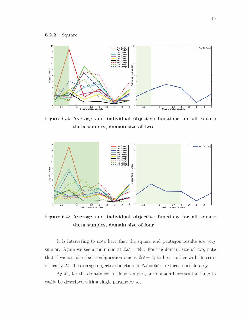
6.2.2 Square
Figure 6.3: Average and individual objective functions for all square
theta samples, domain size of two
Figure 6.4: Average and individual objective functions for all square
theta samples, domain size of four
It is interesting to note here that the square and pentagon results are very
similar. Again we see a minimum at ∆θ = 4δθ. For the domain size of two, note
that if we consider fixel configuration one at ∆θ = δθ to be a outlier with its error
of nearly 20, the average objective function at ∆θ = δθ is reduced considerably.
Again, for the domain size of four samples, our domain becomes too large to
easily be described with a single parameter set.

46
6.3 Expansion along Y-Axis
6.3.1 Pentagon
Figure 6.5: Average and individual objective functions for all pentagon
y samples, domain size of three
Figure 6.6: Average and individual objective functions for all pentagon
y samples, domain size of five
Expanding our domain along the Y-axis provides more insight into the char-
acteristics of the domain than our θ samples. Here we can see a clearly defined
area that is below a certain error threshold. If we consider the central peak of the
domain error, a value of 5 at ∆y = 0 to be our threshold, the average domain of
applicability extends from −2δy to 2.5δy. It is important to note that while the

47
objective function does increase rapidly the further we travel from the domain, the
dynamics of the experiments at the extremities of the Y-Axis were complex, and
often led to large calibration errors with even optimal parameters.
The characteristics of the error seen here is that as we venture outside of the
domain, our error appears to increase at an exponential rate. This suggests that the
domain of applicability for situations in which there is a lateral displacement of the
object is limited to one to two δy, or 8 to 16 millimeters.
6.3.2 Square
Figure 6.7: Average and individual objective functions for all square y
samples, domain size of three

48
Figure 6.8: Average and individual objective functions for all square y
samples, domain size of five
Again, the results for the square domains are similar to those of the pentagon.
Here we see the domain parameters become unstable for a domain size of five, where
no set of parameters can adequately describe the domain so that all models produce
a low error. The domain size of three illustrates a narrow domain of applicability
region.
6.4 Expansion along X-Axis
6.4.1 Pentagon
Figure 6.9: Average and individual objective functions for all pentagon
x samples, domain size of two

49
Figure 6.10: Average and individual objective functions for all pentagon
x samples, domain size of four
The pentagon X-axis domain error is unfortunately marred by the heavy cal-
ibration error near the nominal sample, at ∆x = 0. In addition, the samples near
∆x = 0 produced more complicated trajectories than the samples near ∆x = 5δx,
resulting in higher calibration error even with optimal parameters. This results in a
counter-intuitive result where the error outside of the domain is less than the error
inside it. However, if we remove the outlier calibration error from fixel configuration
4, δx = 0, we observe a more reasonable result. The domain size of four suffers from
the same phenomenon.

50
6.4.2 Square
Figure 6.11: Average and individual objective functions for all square x
samples, domain size of two
Figure 6.12: Average and individual objective functions for all square x
samples, domain size of four
The square domain illustrates a clear domain of applicability. For a domain
size of two, an error threshold of 2.1 extends the domain of applicability to ∆x = 3δx,
and an error threshold of 2.15 extends the domain of applicability to ∆x = 4δx. The
domain size of four produces a very narrow domain of applicability.

51
6.4.3 Absolute and Relative Domain Error
For the preceding analysis, only the absolute error was considered in conjectur-
ing the domain of applicability. However, as was discussed in the previous chapter,
even with optimal parameters, each sample carries calibration error. In figure 6.5
we again show the calibration error for the domain parameters in relation to the
calibration error for the optimal parameters for all samples along the X axis, with
the square.
Figure 6.13: Domain objective function relative to optimal parameter ob-
jective function for all square theta samples, domain size of
2
Comparing this to figure 6.3, we see that the relative error for the domain is
fairly low in comparison to the rest of the samples.
6.5 Possible Sources of Experimental Error
It should be noted that over the course of the experiment, small grooves and
notches formed in the sides of the objects. Occassionally, the actuator head would
become lodged in one of these notches during the course of experimentation. This
may have influenced our simulator to consider very high µs parameters as valid, since
to an outside observer, the coefficient of friction would appear to increase in this

52
case. One possible solution for future experiments may be to replace the copper tape
covering the sides of the objects with a more rigid and durable conductive material,
such as an aluminum or steel sheet.
Another possible source of experiment error was that the lighting in the ex-
periment room changed as experiments were conducted at all hours of the day. This
may have made a small impact on the localization of the colored stickers that are
used to identify the object, fixel and actuator position.

CHAPTER 7
CONCLUSION
This thesis aimed to explore the space of our planar testbed system in terms of ap-
plicability to simulation. By characterizing this domain of applicability, dVC2d, an
accurate physical simulator can be used more effectively and with more sensitivity to
certain aspects of a simulation problem under investigation. The results presented
highlight certain situations in which our physical simulation is appropriate as an
accurate model, and scenarios in which it cannot be relied upon. By examining
expansions along the orthogonal axis of a proposed space of initial object configura-
tions, simulations that model grasping trajectories can gain a better understanding
of how small changes might effect grasp success rates.
The important process of calibration remains a large goal for successful physi-
cal modeling through simulation using dVC2d. In particular, parallellization of the
the optimization search on a feasible scale is a goal that must be pursued in order
to allow for accurate predictive capabilities in a reasonable amount of time. For a
system that must make such predictions on-the-fly, a possible avenue to pursue is
an increase in the time step of the simulator, thereby sacrificing a certain degree of
accuracy for quick results.
The next logical step to pursue for exploring the domain of applicability is
to investigate the space in which dVC3d becomes an acceptable predictor. dVC3d,
the three dimensional version of dVC2d, uses the same formulation as the two-
dimensional model. Since the space of system parameters is so much greater in
three dimensions, additional reductions and simpllifications will need to be made in
order to produce a feasible exploratory framework for dVC3d.
A search for other, possibly more appropriate system models may be useful as
well in producing a more accurate model for both dVC2d and dVC3d. In addition
to parametric modelling of a system, a non-parametric modelling approach to the
planar system may prove to be a worthwhile endeavor. Non-parametric methods
typically allow for more generality than parametric models, and so can account
53

54
for small disturbances and experiment error when used in conjuction with them.
Regression approaches, borrowed from the field of system identification may also
prove to be accurate and robust. In particular, the autocorrelation moving average
approach from system identification may be a good technique for our system model,
since it involves noisy time-interval data.
As a more exotic approach to system identification, machine learning ap-
proaches could in principle be utilized to help identify system parameters by using
a set of system experiments as training data. Bayesian networks represent one class
of machine learning algorithms that may be appropriate for such a task. Hidden
Markov Models may also be used to model a system in which the underlying pa-
rameters are unknown. Particle filters have already successfully been implemented
in determining system parameters for the planar testbed system[16].
For a more complete exploration of the dVC2d, and in general, 2D physi-
cal simulation domain of applicability, a more comprehensive sampling scheme is
required. While the planar testbed experiments space is very large, if the sam-
pling method could be automated for the planar testbed, an exhaustive number of
samples could be drawn from this space. Such a sampling scheme could provide a
low-dispersion sample set that would be a definitive source for sensitivity analysis.
This type of analysis would provide useful predictive information for many planar
manipulation tasks, as well as possibly three-dimensional manipulation tasks.
Generalization of this work may be applied to other system that require iden-
tification, including estimations of other physical parameters like weight, center of
mass and moment of inertia.
The planar testbed is a useful tool, and can be utilized to a great extent
toward two-dimensional problems that may generalize naturally to everyday, three-
dimensional problems. By examining a more simple version of a complicated prob-
lem, a more comprehensive analysis can be made. An understanding of the problem
in this reduced-dimension allows for a knowledgable attempt at the real-world ver-
sion, where a vision system cannot always capture the entire state of the system.
Further research with the planar testbed is undoubtedly necessary for progression
with grasping and manipulation prediction and execution, and has certainly proven

55
to be a valuable tool.

REFERENCES
[1] D. Tong, “Classical dynamics,” class notes for Mathematical Tripos Part II,Department of Applied Mathematics and Theoretical Physics, University ofCambridge, Nov. 2, 2004.
[2] A. Rodriguez, M. Mason, and S. Ferry, “From caging to grasping,” in Proc. ofRobotics: Science and Systems VII, (Los Angeles, CA), Jun. 2011.
[3] M. R. Dogar and S. Srinivasa, “A framework for push-grasping in clutter,” inProc. of Robotics: Science and Systems VII, (Los Angeles, CA), Jun. 2011.
[4] M. Dogar and S. Srinivasa, “Push-grasping with dexterous hands: Mechanicsand a method,” in 2010 IEEE/RSJ Int. Conf. on Intelligent Robots andSystems (IROS), pp. 2123 –2130, Oct. 2010.
[5] C. Kemp, A. Edsinger, and E. Torres-Jara, “Challenges for robotmanipulation in human environments [grand challenges of robotics],” IEEERobot. Automat. Mag., vol. 14, pp. 20 –29, Mar. 2007.
[6] B. Len, S. Ulbrich, R. Diankov, G. Puche, M. Przybylski, A. Morales,T. Asfour, S. Moisio, J. Bohg, and J. Kuffner, OpenGRASP: A Toolkit forRobot Grasping Simulation, vol. 6472 LNAI, pp. 109–120. Springer, 2010.
[7] A. Miller and P. Allen, “Graspit! a versatile simulator for robotic grasping,”IEEE Robot. Automat. Mag., vol. 11, pp. 110 – 122, Dec. 2004.
[8] D. Rosen and K. James, “Openrave: A planning architecture for autonomousrobotics,” Tech. Rep. CMU-RI-TR-08-34, Robotics Institute, Pittsburgh, PA,Jul. 2008.
[9] J. A. Marvel and W. S. Newman, “Model-assisted stochastic learning forrobotic applications,” IEEE Trans. Autom. Sci. Eng., vol. 8, pp. 835 –845,Oct. 2011.
[10] Z. Lu, J. Sun, and K. Butts, “Linear programming svm-arma with applicationin engine system identification,” IEEE Trans. Autom. Sci. Eng., vol. 8,pp. 846 –854, Oct. 2011.
[11] L. Zhang, J. Betz, and J. C. Trinkle, “Comparison of simulated andexperimental grasping actions in the plane,” in 1st Joint Int. Conf. onMultibody System Dynamics, Jun. 2010.
56

57
[12] J. Y. Bouguet, “Camera calibration toolbox for Matlab.”http://www.vision.caltech.edu/bouguetj/calib doc/index.html, 2008. DateLast Accessed, 11/01/2011.
[13] S. Berard, J. C. Trinkle, B. Nguyen, B. Roghani, J. Fink, and V. Kumar,“davinci code: A multi-model simulation and analysis tool for multi-bodysystems,” in 2007 IEEE Int. Conf. on Robotics and Automation, pp. 2588–2593, Apr. 2007.
[14] M. C. Ferris and T. S. Munson, “Interfaces to path 3.0: Design,implementation and usage,” Computational Optimization and Applications,vol. 12, pp. 207–227, 1999. 10.1023/A:1008636318275.
[15] B. M. Adams, J. W. Bohnhoff, Dalbey, et al., “Dakota, a multilevel parallelobject-oriented framework for design optimization, parameter estimation,uncertainty quantification, and sensitivity analysis. ver 5.1 users manual.,”Tech. Rep. SAND2010-2183, Sandia National Laboratories, Livermore, CA,Dec. 2009.
[16] L. Zhang and J. Trinkle, “Exploring the application of particle filters tograsping acquisition with visual and tactile occlusion,” Tech. Rep. 10-09,Department of Computer Science, Rensselaer Polytechnic Institute, 2010.

APPENDIX A
Matlab CCNI Calibration Interface Technical Notes
A.1 Landing Pad Setup
Using the Matlab interface to the CCNI supercomputing cluster requires an
understanding of the various files and directory structure on the remote machine
so that correct operation is possible. Also, an understanding of the various Matlab
files used in the process of remote calibration is important for correct calibration
processing, and keeping data from being corrupted. The following technical notes
elaborate these issues.
A.2 Directory structure on Landing Pad
Users who are granted an account on CCNI are given a data folder for their
respective project. The directory structure of this folder must be correct for the
Matlab interface to correctly setup and submit jobs for SLURM and Dakota to
process. Below is a directory tree showing the necessary directory structure of this
data subdirectory:
58

59
Figure A.1: CCNI remote directory structure
A.3 Matlab File and Procedure for Calibration
Every calibration that is created by a user is given a unique file, named
calibration XX, where XX represents a unique identifier for this calibration.This
file contains all the relevant information regarding a particular calibration, including
the SLURM job id, experiments that are being calibrated against, the final objective
function and the final calibrated parameters. If a user is using the Matlab inter-
face to perform remote calibration functions, the general lifecycle that a calibration
undergoes is:
1. A user select a set of 1 or more experiments to queue for calibration by using
QueueExperimentForCalibrationSetup.m. This will create calibration XX
for this calibration. An entry will also be created in the calibrations table in
the 2dgad.
2. Once queued, a user may set up the prerequisites necessary for Dakota to oper-
ate on the remote file system by executing RunExperimentCalibrationSetup.m.

60
3. Once the prerequisites have been set up, all that is left is to submit the cali-
bration job to SLURM using RunSubmitCalibration.m.
4. After the job has completed, run Collect Completed Calibration Results.m
to copy resulting parameters from all completed calibrations to the calibration
files for each respective calibration.
5. RetrieveCalibratedExperimentParameters.m will take these calibration files
and transfer them to the experimenter’s local machine, where they will be pro-
cessed and inserted into the 2dgad database.

APPENDIX B
Step-by-step Guide to Conducting Experiments
This appendix provides a step-by-step guide to conducting experiments on the planar
testbed. The instructions are general to accomodate different fixel configurations,
object geometries and pusher geometries It assumes that the experimenter has the
necessary apparatus and equipment, however, the general procedure is valid for
similar experimental testbeds.
B.1 Step 1: Preparing the testbed system
B.1.1 Configuring Matlab
All experiments are conducted through Matlab, so Matlab must be running
on the experimenter’s computer. First, checkout the 2dTestbed Matlab code folder
from the lab SVN, at svn+ssh://grasp.robotics.cs.rpi.edu/var/svn/repo/2dTestbed.
Add this folder to the Matlab path by right clicking the folder from within the Mat-
lab environment and selecting “Add to Path → Selected Folders and Subfolders”.
All necessary experiment code should now be loaded.
In order to successfully log experiments, three configuration items in
2dTestbed/configure.m must be specified.
• videoPath must be set to a folder available for storing experiment videos,
• imagePath must be set to a folder available for storing extracted experiment
images and
• dataPath must be set to a folder available for storing experiment and simula-
tion plots.
Save these changes.
B.1.2 Initializing the Linear Actuator
The PC that controls the linear actuator must also be on. The experimenter
should at this time connect to the linear actuator PC via Remote Desktop Con-
61

62
nection (mstsc.exe). While remoting into the linear actuator PC, the experimenter
should start the TBVST program, which is the application used to control the linear
actuator.
Figure B.1: The TBVST program icon, and program GUI
In the TBVST program window, select “Servo ON” to turn the linear actuator
on. Leave the remote desktop connection open, as it will be used in a later step to
perform our experiment.
B.1.3 Initializing the Arduino
Ensure that the arduino is plugged into the experimenter’s computer. Load up
the arduino programming enviroment, and open tactile arduino program.pde,
located in 2dTestbed/Extras/tactile arduino program/. Upload this program to
the arduino. Check to see which port the arduino is operating on by selecting
“Tools → Serial Port” from the menu bar of the arduino programming environ-
ment. Then navigate to 2dTestbed/Extras/Capture Video And Tactile/ and open
Capture Video And Tactile.m. Replace the “port” variable with whatever port
the arduino was observed to be connected to.
B.1.4 Initializing the webcam
Ensure that the webcam is accessible by navigating to Matlab’s start menu,
and select “Start → Toolboxes → Image Acquisition Toolbox → Image Acquisiton

63
Tool”. Select RGB1280 X 720 in the left navigation pane, and click “Start Preview”.
A preview of the testbed from the camera should appear.
Figure B.2: Matlab’s Image Acquisition Tool
B.2 Step 2: Setting up the initial configuration
Once the system has been initialized and set up, the experimenter must setup
the initial configuration of the testbed for their experiment. Unscrew the fixels from
the testbed and screw them into the desired fixel locations. Select an object, and
an initial object position and orientation. Navigate to 2dTestbed/Extras/Overlay/,
and locate Overlay With Coords.m. Provide this function with the three param-
eters mentioned, and an interactive overlay of the testbed with the initial object
configuration outlined will appear. Use this streaming overlay to manually position
the object in the outlined area. Press “Ctrl + C” to exit the overlay.
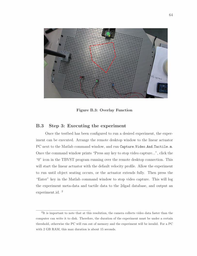
64
Figure B.3: Overlay Function
B.3 Step 3: Executing the experiment
Once the testbed has been configured to run a desired experiment, the exper-
iment can be executed. Arrange the remote desktop window to the linear actuator
PC next to the Matlab command window, and run Capture Video And Tactile.m.
Once the command window prints “Press any key to stop video capture...”, click the
“0” icon in the TBVST program running over the remote desktop connection. This
will start the linear actuator with the default velocity profile. Allow the experiment
to run until object seating occurs, or the actuator extends fully. Then press the
“Enter” key in the Matlab command window to stop video capture. This will log
the experiment meta-data and tactile data to the 2dgad database, and output an
experiment id. 2
2It is important to note that at this resolution, the camera collects video data faster than the
computer can write it to disk. Therefore, the duration of the experiment must be under a certain
threshold, otherwise the PC will run out of memory and the experiment will be invalid. For a PC
with 2 GB RAM, this max duration is about 15 seconds.

65
B.4 Step 4: Processing the results
Once the experiment has been executed, run processExperiment.m to ex-
tract the object and actuator trajectory, as well as the fixel locations to the 2dgad.
This function requires the experiment id that was outputted after executing the
experiment. Once this completes, all experiment data is now in the 2dgad.
B.5 Step 5: Calibrating the results
At this point, the experimenter may wish to calibrate this experiment to de-
termine the optimal parameters that fit the dVC2d simulation that corresponds
to this experiment. To do so, run the steps specified in Appendix A. If the re-
sults appear to have found a local minimum in parameter space, it is useful to
run Piecewise Calibration Single Exp.m, located in /2dTestbed/Extras/ Piece-
wise Calibration. This function requires the experiment id, maximum number of
iterations for the search, as well as the number of contractions to perform. This will
perform a similar pattern search on this experiment that is executed on the CCNI
cluster, and log the new calibrated results to the 2dgad.
B.6 Step 6: Simulating the results
To simulate this experiment with the calibrated system parameters, locate the
calibration entry in the calibration table corresponding to this calibration, and select
the system parameter id. Run runSimulation.m with this system parameter id and
the experiment id of the desired experiment. This will run the simulation, log it to
the database, and output a simulation id. The simulation may then be visualized
against the experimental data using the compare.m script in /2dTestbed/Launch/.
Simply specify the experiment id and simulation id in the two variables at the top
of the script, and execute it.
In the case that there are multiple calibrations for an experiment or set of
experiments, run Best Params For Exps By Max Error.m to identify the best pa-
rameters for these experiments.

APPENDIX C
SOURCE CODE LISTINGS
C.1 Calibration Source Code
showstringspaces
#!/ bin / bash
# This s c r i p t w i l l check the c a l i b r a t i o n queue f o l d e r and se tup
# any and a l l p r e r e q u i s i t e s necessary f o r c a l i b r a t i o n
c a l i b r a t i o n s t o b e s e t u p=/gp f s / smal l /SDRG/home/SDRGmacw/data/
Cal ibrat ions To Be Setup /∗
c a l i b r a t i o n s t o b e s e t u p p a t h=/gp f s / smal l /SDRG/home/SDRGmacw/data/
Cal ibrat ions To Be Setup
ca l i b r a t i on s t o b e subm i t t e d pa th=/gp f s / smal l /SDRG/home/SDRGmacw/data/
Cal ibrat ions To Be Submitted
c a l i b r a t i o n i n i t i a l p a r ame t e r s p a t h=”/ gp f s / smal l /SDRG/home/SDRGmacw/
data/ Ca l i b r a t i o n I n i t i a l P a r ame t e r s /”
da t a d i r e c t o r y=/gp f s / smal l /SDRG/home/SDRGmacw/data/ Ca l i b r a t i on s /
for f i l e in $ c a l i b r a t i o n s t o b e s e t u p
do
################### Extrac t c a l i b r a t i o n queue f i l e f i l ename
###########################
echo ”Extract ing f i l ename o f c a l i b r a t i o n queue f i l e . . . ”
f i l ename=$ ( basename ” $ f i l e ” )
ex t ens i on=$ f i l ename##∗.
f i l ename=$ f i l ename%.∗
################### Read con ten t s o f c a l i b r a t i o n queue f i l e
###########################
66

67
echo ”Reading c a l i b r a t i o n queue f i l e . . . ”
c a l i b r a t i o n f i l e c o n t e n t s =‘cat $ f i l e ‘
echo ”Experiments f o r t h i s c a l i b r a t i o n are : ”
echo $ c a l i b r a t i o n f i l e c o n t e n t s
################## Read i n i t i a l parameter f i l e
###########################
i n i t i a l p a r am s f i l e=”$ c a l i b r a t i o n i n i t i a l p a r ame t e r s p a t h $
f i l ename i n i t i a l p a r am s ”
echo ”Reading i n i t i a l parameters f i l e ”
t r i p od r ad i u s=$ (awk ’ pr in t $1 ’ $ i n i t i a l p a r am s f i l e )
f i x e l f r i c t=$ (awk ’ pr in t $2 ’ $ i n i t i a l p a r am s f i l e )
o b j e c t f r i c t=$ (awk ’ pr in t $3 ’ $ i n i t i a l p a r am s f i l e )
a c t u a t o r f r i c t=$ (awk ’ pr in t $4 ’ $ i n i t i a l p a r am s f i l e )
################### Make f o l d e r f o r t h i s c a l i b r a t i o n
##############################
echo ”Making $ f i l ename d i r e c t o r y . . . ”
n ew c a l i b r a t i o n f o l d e r=” $da ta d i r e c t o ry$ f i l e name ”
# Make a d i r e c t o r y in ”data ” corresponding to t h i s c a l i b r a t i o n
mkdir ” $n ew c a l i b r a t i o n f o l d e r ”
chmod 770 $n ew c a l i b r a t i o n f o l d e r
# Give permiss ions to e v e r y t h in g
chmod 770 ∗
############## Create and a l l s c r i p t s f o r t h i s c a l i b r a t i o n
###############

68
#Sp l i t a l l exper iments in c a l i b r a t i o n f i l e i n t o array
exp array=($ c a l i b r a t i o n f i l e c o n t e n t s // / )
#Move to our new c a l i b r a t i o n d i r e c t o r y
cd ” $n ew c a l i b r a t i o n f o l d e r ”
#Create p r e r e q u i s i t e s c r i p t s / f i l e s f o r Dakota
. . . / . . / Produce Submit Job Scr ipt . sh ” $n ew c a l i b r a t i o n f o l d e r ” ”$#
exp array [@] ” > ” submit job . sh”
. . . / . . / Produce S ta r t Sc r i p t . sh > ” s t a r t . sh”
. . . / . . / Produce Template Scr ipt . sh > ” template ”
. . . / . . / Produce Dakota Parameters Scr ipt . sh $ t r i p od r ad i u s
$ f i x e l f r i c t $ o b j e c t f r i c t $ a c t u a t o r f r i c t 0 . 5 > ”
dakota dvc NGOpt PatternSearch m . in ”
. . . / . . / Produce Video Sequence Scr ipt . sh ” $ c a l i b r a t i o n f i l e c o n t e n t s ”
> ”videoSeq m . sh”
. . . / . . / Produce Simparams Script . sh > ”simparams . txt ”
#I f our c a l i b r a t i o n has on ly one experiment , do the s i n g l e experiment
procedure .
#Otherwise , do the mu l t i p l e experiment c a l i b r a t i o n procedure
i f [ $#exp array [@] = 1 ]
then
. . . / . . / P roduc e S imu l a t o r S c r i p t S i ng l e Ca l i b r a t i on . sh ”
$ c a l i b r a t i o n f i l e c o n t e n t s ” > ” s imu l a t o r s c r i p t ”
. . . / . . / Produce Submit Job Scr ipt . sh ” $n ew c a l i b r a t i o n f o l d e r ”
”$#exp array [@] ” ”240” > ” submit job . sh”
else
. . . / . . / P roduc e S imu l a t o r S c r i p t Mu l t i p l e Ca l i b r a t i on . sh > ”
s imu l a t o r s c r i p t ”
. . . / . . / Produce Submit Job Scr ipt . sh ” $n ew c a l i b r a t i o n f o l d e r ”
”$#exp array [@] ” ”600” > ” submit job . sh”
f i
chmod 770 ∗

69
############# Move c a l i b r a t i o n f i l e to ” Ca l i b r a t i on s to be Setup”
##########################
mv ” $ f i l e ” ” $ c a l i b r a t i on s t o b e subm i t t ed pa th ”
cd $ c a l i b r a t i on s t o b e subm i t t ed pa th
chmod 770 ∗
done
Source Code/Setup Calibration Prerequisites.sh
C.2 Arduino Tactile Program Source Code
showstringspaces
int green p in = 1 ;
int r ed p in = 0 ;
int b lue p in = 2 ;
int th r e sho ld = 900 ;
void setup ( )
S e r i a l . begin (115200) ;
void loop ( )
byte t a c t i l e b y t e = 0 ;
i f ( S e r i a l . a v a i l a b l e ( ) > 0)
int r e d p i n va l = analogRead (0 ) ;
int g r e en p i n va l = analogRead (1 ) ;
int b l u e p i n v a l = analogRead (2 ) ;

70
i f ( r e d p i n va l > th r e sho ld )
t a c t i l e b y t e = t a c t i l e b y t e ˆ 2 ;
i f ( b l u e p i n v a l > th r e sho ld )
t a c t i l e b y t e = t a c t i l e b y t e ˆ 1 ;
i f ( g r e en p i n va l > th r e sho ld )
t a c t i l e b y t e = t a c t i l e b y t e ˆ 4 ;
S e r i a l . wr i t e ( t a c t i l e b y t e ) ;
S e r i a l . f l u s h ( ) ;
Source Code/tactile arduino program.pde
C.3 Testbed Overlay Source Code
showstringspaces
function Overlay ( exp id , ob j t h e t a d e l t a , ob j e c t po s d e l t a ,
f i x e l 1 d e l t a , f i x e l 2 d e l t a , f i x e l 3 d e l t a , a c t po s d e l t a ,
a c t t h e t a d e l t a )
%% I n i t i a l i z e database connect ion
dbConn = database ( ’ 2dgad ’ , ’ r o b o t i c s ’ , ’ s en so rne t ’ , ’ org . p o s t g r e s q l . Dr iver
’ , ’ jdbc : p o s t g r e s q l : // grasp . r o bo t i c s . c s . r p i . edu/ ’ ) ;
% Clean and i n i t i a l i z e camera d r i v e r
video = imaqf ind ;
for i =1: length ( v ideo )
delete ( v ideo ( i ) ) ;
end

71
vid = video input ( ’ winvideo ’ , 1 , ’ RGB24 1280x720 ’ ) ;
v id . TimerPeriod = . 0 4 ;
c on f i gu r e ;
%% Se l e c t a l l exper iments from the database t ha t have not been
processed
unprocessed exp query = [ ’SELECT v i d e o f i l e p a t h FROM experiment WHERE
exper iment id = ’ num2str( exp id ) ] ;
% Execute query
cur so r = exec (dbConn , unprocessed exp query ) ;
f e t cheddata = f e t ch ( cur so r ) ;
v i d e o f i l e p a t h = fe tcheddata . data ( : , 1) ;
%% Check to ensure the v ideo f i l e i s on our computer
f u l l f i l e p a t h = s t r c a t ( videoPath , v i d e o f i l e p a t h ) ;
i f exist ( f u l l f i l e p a t h 1)
%% Retr i eve the image o f the f i r s t v ideo frame
v id eo r eade r = VideoReader ( f u l l f i l e p a t h 1) ;
f i r s t f r am e = read ( v ideo reader , 1) ;
else
fprintf ( ’ Image not on computer ’ ) ;
return ;
end
% Load f i x e l geometry
global pegH SIMPAUSETIME lineWidth ;
B3 = [ 4 .76 −0.00;
4 .53 −1.47;
3 .85 −2.80;
2 .80 −3.85;
1 .47 −4.53;
0 .00 −4.76;
−1.47 −4.53;
−2.80 −3.85;

72
−3.85 −2.80;
−4.53 −1.47;
−4.76 −0.00;
−4.53 1 . 4 7 ;
−3.85 2 . 8 0 ;
−2.80 3 . 8 5 ;
−1.47 4 . 5 3 ;
−0.00 4 . 7 6 ;
1 .47 4 . 5 3 ;
2 .80 3 . 8 5 ;
3 .85 2 . 8 0 ;
4 .53 1 . 4 7 ; ] ;
%% Load o b j e c t geometr i e s
ob j e c t g eomet ry id = ce l l 2mat ( f e t ch (dbConn , sprintf ( ’SELECT
ob j e c t g eomet ry id FROM experiment WHERE exper iment id = %d ’ , exp id
) ) ) ;
a c tuato r geomet ry id = ce l l 2mat ( f e t ch (dbConn , sprintf ( ’SELECT
actuato r geomet ry id FROM experiment WHERE exper iment id = %d ’ ,
exp id ) ) ) ;
objGeometry = PostgresqlToMatlabArray ( ce l l 2mat ( f e t ch (dbConn , sprintf ( ’
SELECT geometry FROM obje c t ac tua to r geomet ry WHERE
ob j e c t a c tua t o r g eome t ry i d = %d ’ , ob j e c t g eomet ry id ) ) ) ) ;
objHeight = ce l l 2mat ( f e t ch (dbConn , sprintf ( ’SELECT he ight FROM
obje c t ac tua to r geomet ry WHERE ob j e c t a c tua t o r g eome t ry i d = %d ’ ,
ob j e c t g eomet ry id ) ) ) ;
actGeometry = PostgresqlToMatlabArray ( ce l l 2mat ( f e t ch (dbConn , sprintf ( ’
SELECT geometry FROM obje c t ac tua to r geomet ry WHERE
ob j e c t a c tua t o r g eome t ry i d = %d ’ , ac tuato r geomet ry id ) ) ) ) ;
actHeight = ce l l 2mat ( f e t ch (dbConn , sprintf ( ’SELECT he ight FROM
obje c t ac tua to r geomet ry WHERE ob j e c t a c tua t o r g eome t ry i d = %d ’ ,
ac tuato r geomet ry id ) ) ) ;
%% Object h e i g h t s
objH = objHeight ;
actH = actHeight ;
%% Load Ca l i b r a t i on parameter

73
% PARAMETERFILENAME i s de f ined in con f i gu r e
ca l ibPara = loadCa l i b r a t i on (PARAMETERFILENAME) ;
%% Set Ex t r i n s i c Parameters
Rc = ca l ibPara . Rc ;
Tc = ca l ibPara . Tc ;
cc = ca l ibPara . cc ;
f c = ca l ibPara . f c ;
kc = ca l ibPara . kc ;
a lpha c = ca l ibPara . a lpha c ;
%% Load experiment coord ina t e s
[ o b j e c t i n i t i a l p o s i t i o n d a t a , . . .
o b j e c t o r i e n t da t a , . . .
a c tua t o r o r i en t da t a , . . .
f i x e l 1 p o s i t i o n d a t a , . . .
f i x e l 2 p o s i t i o n d a t a , . . .
f i x e l 3 p o s i t i o n d a t a , . . .
a c t u a t o r p o s i t i o n da t a ] = Load Experiment Coordinates ( exp id ) ;
%% Se l e c t on ly i n i t i a l c on f i g u r a t i on in format ion
ob j e c t o r i e n t d a t a = ob j e c t o r i e n t d a t a (1 ) ;
o b j e c t i n i t i a l p o s i t i o n d a t a = o b j e c t i n i t i a l p o s i t i o n d a t a ( 1 : 2 ) ;
a c t u a t o r o r i e n t da t a = ac tua t o r o r i e n t da t a 1 ;
a c t u a t o r po s i t i o n da t a = ac tua t o r po s i t i o n da t a (1 , 1 : 2 ) ;
f i x e l 1 p o s i t i o n d a t a = f i x e l 1 p o s i t i o n d a t a ( 1 : 2 ) ;
f i x e l 2 p o s i t i o n d a t a = f i x e l 2 p o s i t i o n d a t a ( 1 : 2 ) ;
f i x e l 3 p o s i t i o n d a t a = f i x e l 3 p o s i t i o n d a t a ( 1 : 2 ) ;
%% Retr i eve current ac tua tor p o s i t i o n and o r i e n t a t i o n
[ p i x e l l o c a t i o n o r i e n t a t i o n p i x e l ] = F ind Actuato r St i cke r ( ) ;
%% Determine o r i e n t a t i on po in t s in r e a l world
r e a l c o o r d c e n t e r = coo rd ina t e Inve r s e ( p i x e l l o c a t i o n ’ , 0 , ca l ibPara ) ;
r e a l c o o r d o r i e n t = coo rd ina t e Inve r s e ( o r i e n t a t i o n p i x e l , 0 , ca l ibPara ) ;
o r i e n t a t i o n v e c t o r = r e a l c o o r d o r i e n t − r e a l c o o r d c e n t e r ;
% Construct t h e t a in r e a l world

74
theta = atan2 ( o r i e n t a t i o n v e c t o r (2 ) , o r i e n t a t i o n v e c t o r (1 ) ) ;
% Determine t h e t a d i f f e r e n c e
t h e t a d i f f = theta − a c t ua t o r o r i e n t da t a ;
% Rotate everybody by t h e t a d i f f in the r e a l world
R = [ cos ( t h e t a d i f f ) −sin ( t h e t a d i f f ) ; sin ( t h e t a d i f f ) cos ( t h e t a d i f f )
] ;
o b j e c t i n i t i a l p o s i t i o n d a t a = R∗ o b j e c t i n i t i a l p o s i t i o n d a t a ’ ;
a c t u a t o r po s i t i o n da t a = R∗ a c tua t o r po s i t i on da t a ’ ;
f i x e l 1 p o s i t i o n d a t a = R∗ f i x e l 1 p o s i t i o n d a t a ’ ;
f i x e l 2 p o s i t i o n d a t a = R∗ f i x e l 2 p o s i t i o n d a t a ’ ;
f i x e l 3 p o s i t i o n d a t a = R∗ f i x e l 3 p o s i t i o n d a t a ’ ;
a c t u a t o r o r i e n t da t a = theta ;
o b j e c t o r i e n t d a t a = ob j e c t o r i e n t d a t a + t h e t a d i f f ;
o b j e c t i n i t i a l p o s i t i o n d a t a = o b j e c t i n i t i a l p o s i t i o n d a t a ’ ;
a c t u a t o r po s i t i o n da t a = ac tua t o r po s i t i on da t a ’ ;
f i x e l 1 p o s i t i o n d a t a = f i x e l 1 p o s i t i o n d a t a ’ ;
f i x e l 2 p o s i t i o n d a t a = f i x e l 2 p o s i t i o n d a t a ’ ;
f i x e l 3 p o s i t i o n d a t a = f i x e l 3 p o s i t i o n d a t a ’ ;
%% Adjust parameters based on d e l t a s
o b j e c t i n i t i a l p o s i t i o n d a t a = o b j e c t i n i t i a l p o s i t i o n d a t a +
ob j e c t p o s d e l t a ;
o b j e c t o r i e n t d a t a = ob j e c t o r i e n t d a t a + ob j t h e t a d e l t a ;
a c t u a t o r o r i e n t da t a = ac tua t o r o r i e n t da t a + a c t t h e t a d e l t a ;
f i x e l 1 p o s i t i o n d a t a = f i x e l 1 p o s i t i o n d a t a + f i x e l 1 d e l t a ;
f i x e l 2 p o s i t i o n d a t a = f i x e l 2 p o s i t i o n d a t a + f i x e l 2 d e l t a ;
f i x e l 3 p o s i t i o n d a t a = f i x e l 3 p o s i t i o n d a t a + f i x e l 3 d e l t a ;
a c t u a t o r po s i t i o n da t a = ac tua t o r po s i t i o n da t a + a c t p o s d e l t a ;
a c t u a t o r o r i e n t da t a = ac tua t o r o r i e n t da t a + a c t t h e t a d e l t a ;
%% Ca l cu l a t e the corner in r e a l world
oCorner = cornerConvers ion ( o b j e c t i n i t i a l p o s i t i o n d a t a ,
ob j e c t o r i e n t da t a , objGeometry ’ ) ;

75
aCorner = cornerConvers ion ( a c tua t o r po s i t i on da t a , a c tua t o r o r i en t da t a
, actGeometry ’ ) ;
f1Corner = cornerConvers ion ( f i x e l 1 p o s i t i o n d a t a , 0 , B3 ’ ) ;
f2Corner = cornerConvers ion ( f i x e l 2 p o s i t i o n d a t a , 0 , B3 ’ ) ;
f3Corner = cornerConvers ion ( f i x e l 3 p o s i t i o n d a t a , 0 , B3 ’ ) ;
%% Pro jec t to image space
oCorner (3 , : ) = objH ;
aCorner (3 , : ) = actH ;
f1Corner (3 , : ) = pegH ; f2Corner (3 , : ) = pegH ; f3Corner (3 , : ) = pegH ;
oCorner = p r o j e c t p o i n t s 2 ( oCorner , r od r i gue s (Rc) , Tc , fc , cc , kc ,
a lpha c ) ;
aCorner = p r o j e c t p o i n t s 2 ( aCorner , r od r i gue s (Rc) , Tc , fc , cc , kc ,
a lpha c ) ;
f1Corner = p r o j e c t p o i n t s 2 ( f1Corner , r od r i gue s (Rc) , Tc , fc , cc , kc ,
a lpha c ) ;
f2Corner = p r o j e c t p o i n t s 2 ( f2Corner , r od r i gue s (Rc) , Tc , fc , cc , kc ,
a lpha c ) ;
f3Corner = p r o j e c t p o i n t s 2 ( f3Corner , r od r i gue s (Rc) , Tc , fc , cc , kc ,
a lpha c ) ;
aCorner c t r = mean( aCorner ’ ) ;
p i x e l l o c a t i o n = round( p i x e l l o c a t i o n ) − aCorner c t r ;
[ f v e r t e x h e i g h t f v e r t e x w id th ] = s ize ( f1Corner ) ;
[ o b j e c t v e r t e x h e i g h t ob j e c t v e r t ex w id th ] = s ize ( oCorner ) ;
[ a c t ua t o r v e r t e x h e i gh t ac tua to r ve r t ex w id th ] = s ize ( aCorner ) ;
%% Trans la te a l l p i x e l s by d i f f e r e n c e in po s i t i o n
oCorner (1 , : ) = oCorner (1 , : ) + ones (1 , ob j e c t v e r t ex w id th ) ∗
p i x e l l o c a t i o n (1 ) ;
oCorner (2 , : ) = oCorner (2 , : ) + ones (1 , ob j e c t v e r t ex w id th ) ∗
p i x e l l o c a t i o n (2 ) ;
aCorner (1 , : ) = aCorner (1 , : ) + ones (1 , a c tua to r ve r t ex w id th ) ∗
p i x e l l o c a t i o n (1 ) ;
aCorner (2 , : ) = aCorner (2 , : ) + ones (1 , a c tua to r ve r t ex w id th ) ∗
p i x e l l o c a t i o n (2 ) ;

76
f1Corner (1 , : ) = f1Corner (1 , : ) + ones (1 , f v e r t e x w id th ) ∗
p i x e l l o c a t i o n (1 ) ;
f1Corner (2 , : ) = f1Corner (2 , : ) + ones (1 , f v e r t e x w id th ) ∗
p i x e l l o c a t i o n (2 ) ;
f2Corner (1 , : ) = f2Corner (1 , : ) + ones (1 , f v e r t e x w id th ) ∗
p i x e l l o c a t i o n (1 ) ;
f2Corner (2 , : ) = f2Corner (2 , : ) + ones (1 , f v e r t e x w id th ) ∗
p i x e l l o c a t i o n (2 ) ;
f3Corner (1 , : ) = f3Corner (1 , : ) + ones (1 , f v e r t e x w id th ) ∗
p i x e l l o c a t i o n (1 ) ;
f3Corner (2 , : ) = f3Corner (2 , : ) + ones (1 , f v e r t e x w id th ) ∗
p i x e l l o c a t i o n (2 ) ;
%% I n i t i a l i z e webcam
t r i g g e r c o n f i g ( vid , ’manual ’ ) ;
s t a r t ( v id ) ;
%% Must send k i l l s i g n a l to terminate t h i s loop once o b j e c t i s in
p o s i t i o n
while t rue
%% Retr i eve frame
data = getsnapshot ( vid ) ;
%% Disp lay image
imshow ( data ) ;
hold on ;
%% Overlay o b j e c t s on image
sHnd1 = plot (1 , 1 , ’ r ’ , ’ LineWidth ’ , l ineWidth ) ;
sHnd2 = plot (1 , 1 , ’ b ’ , ’ LineWidth ’ , l ineWidth ) ;
sHnd3 = plot (1 , 1 , ’ g ’ , ’ LineWidth ’ , l ineWidth ) ;
sHnd4 = plot (1 , 1 , ’ g ’ , ’ LineWidth ’ , l ineWidth ) ;
sHnd5 = plot (1 , 1 , ’ g ’ , ’ LineWidth ’ , l ineWidth ) ;
% Plot r e c t an g l e
p lo tRectang l e ( oCorner , sHnd1 ) ;

77
p lo tRectang l e ( aCorner , sHnd2 ) ;
p lo tRectang l e ( f1Corner , sHnd3 ) ;
p lo tRectang l e ( f2Corner , sHnd4 ) ;
p lo tRectang l e ( f3Corner , sHnd5 ) ;
hold o f f ;
end
end
Source Code/Overlay.m
C.4 Video and Tactile Capture Source Code
showstringspaces
function Capture Video And Tact i le ( v i d e o f i l e p a t h e nd )
% This func t i on w i l l capture v ideo and t a c t i l e data u n t i l a user
% manually t e rminates the func t i on
c on f i gu r e ( ) ;
% g l o b a l v ideoPath
global videoPath
% Path to v i deo s
v i d e o f i l e p a t h = s t r c a t ( videoPath , v i d e o f i l e p a t h e nd ) ;
% Set image frame memory l im i t
%imaqmem(imaqmem( ’ Avai lphys ’ ) ) ;
% I n i t i a l i z e v ideo o b j e c t
vid = video input ( ’ winvideo ’ , 1 , ’ RGB24 1280x720 ’ ) ;
% Get v ideo source
s r c = g e t s e l e c t e d s ou r c e ( vid ) ;

78
% Set frames per t r i g g e r to i n f i n i t e ( f o r v ideo )
vid . FramesPerTrigger = Inf ;
% Preview the sho t
%preview ( v id ) ;
% Set focus to manual so t ha t we don ’ t r e f o cu s wh i l e we are f i lm in g
s r c . FocusMode = ’manual ’ ;
% Save v ideo to d i s k
vid . LoggingMode = ’ d i sk ’ ;
% Se t t i n g s f o r f i l e and v ideo stream i n i t i a l i z a t i o n to d i s k
diskLogger = a v i f i l e ( v i d e o f i l e p a t h , ’ Compression ’ , ’None ’ , ’ Qual i ty ’ ,
75 , ’ keyframepersec ’ , 2 . 14 , ’FPS ’ , 30) ;
v id . DiskLogger = diskLogger ;
%Ce l l array to ho ld t a c t i l e b y t e s
%t a c t i l e b y t e s = c e l l (1) ;
global t a c t i l eBy t e s
t a c t i l eBy t e s = c e l l ( 0 ) ;
% Custom s e r i a l connect ion to Arduino . F i r s t d e l e t e any pre−e x i s t i n g
% connect ions
delete ( i n s t r f i n d ( ’ Port ’ , ’COM4’ ) )
s e r i a l o b j e c t = s e r i a l ( ’COM4’ , ’BAUD’ , 115200) ;
fopen ( s e r i a l o b j e c t ) ;
fpr intf ( ’ Opening S e r i a l Connection . . . \ n ’ ) ;
pause (1 ) ;
fpr intf ( ’ S e r i a l Connection Opened\n ’ ) ;
% Arduino o b j e c t . Attempt to d e l e t e b e f o r e we use i t to be s a f e .
%d e l e t e ( i n s t r f i n d ( ’ Port ’ , ’COM4’ ) )
%ardu ino ob j e c t = arduino ( ’COM4’ ) ;

79
% Set c a l l b a c k func t i on
set ( vid , ’ FramesAcquiredFcnCount ’ , 1) ;
%se t ( vid , ’ FramesAcquiredFcn ’ , ’ Query Tac t i l e Sensor Ca l l back ’ ,
t a c t i l e b y t e s , a r du ino ob j e c t ) ;
vid . FramesAcquiredFcn = ’ Query Tact i l e Senso r Ca l lback ’ , s e r i a l o b j e c t
;
t ry
% Sta r t the v ideo
s t a r t ( v id ) ;
% This w i l l wai t f o r keyboard input − Press any key to s top v ideo
capture
evalResponse = input ( ’ Press any key to stop video capture ’ ) ;
%Wait u n t i l our t a c t i l e data syncs wi th our v ideo data
while ( length ( t a c t i l eBy t e s ) ˜= vid . FramesAcquired )
pause ( . 0 005 ) ;
end
% Stop the v ideo
stop ( vid ) ;
% Write to d i s k
while ( v id . DiskLoggerFrameCount ˜= vid . FramesAcquired )
pause (1 ) ;
end
diskLogger = close ( v id . DiskLogger ) ;
% I f t h e r e s an error anywhere , e x i t so we don ’ t save to the database
catch
fpr intf ( ’Memory e r r o r ! Not l ogg ing t h i s experiment to the database !
’ )
return ;
end

80
% Returned t a c t i l e b y t e s
t a c t i l e b y t e s = t a c t i l eBy t e s ;
t a c t i l e b y t e s = ce l l 2mat ( t a c t i l e b y t e s ) ;
% Dispose o f arduino o b j e c t
%d e l e t e ( i n s t r f i n d ( ’ Port ’ , ’COM4’ ) )
%Close our s e r i a l connect ion
fc lose ( s e r i a l o b j e c t ) ;
f inalContactMode = t a c t i l eBy t e s ( length ( t a c t i l eBy t e s ) ) ;
fpr intf ( ’Number o f t a c t i l e bytes acqu i red : ’ )
fpr intf (num2str( length ( t a c t i l eBy t e s ) ) )
fpr intf ( ’ \nNumber o f frames acqu i red : ’ )
fpr intf (num2str( v id . FramesAcquired ) ) ;
% I f the number o f t a c t i l e b y t e s e qua l s the number o f frames acquired ,
send
% eve r y t h in g to the database
i f ( length ( t a c t i l eBy t e s ) ˜= vid . FramesAcquired )
fpr intf ( ’Frame count and number o f t a c t i l e reads don ’ ’ t match !
Ex i t ing . ’ )
else
dbExportExperimentWithTactileNoPrompt ( v i d e o f i l e p a t h end ,
t a c t i l eBy t e s , f inalContactMode ) ;
end
end
Source Code/Capture Video And Tactile.m
C.5 MATLAB Pattern Search
showstringspaces
t ry

81
matlabpool close
catch ex
fpr intf ( ’ \nMatlab pool not open ’ ) ;
end
t ry
matlabpool l o c a l 7
catch
fpr intf ( ’ \nMatlab pool cannot open ’ ) ;
end
% I n i t i a l i z e database connect ion
dbConn = database ( ’ 2dgad ’ , ’ r o b o t i c s ’ , ’ s en so rne t ’ , ’ org . p o s t g r e s q l . Dr iver
’ , ’ jdbc : p o s t g r e s q l : // grasp . r o bo t i c s . c s . r p i . edu/ ’ ) ;
%% Se l e c t a l l exper iments in our sample s e t
query = ’SELECT exper iment id , ob j e c t g eomet ry id FROM experiment WHERE
exper iment id > 170 ’ ;
r e s u l t = ce l l 2mat ( f e t ch (dbConn , query ) ) ;
exper iments = r e s u l t ( : , 1) ;
ob j e c t g eomet ry id = r e s u l t ( : , 2) ;
d e l t a u f = . 0 5 ;
de l ta up = . 0 5 ;
d e l t a u s = . 0 5 ;
d e l t a R t r i = 2 ;
%% For each o f the experiments , s e l e c t the b e s t params
par f o r j =1: length ( exper iments )
[ best params ( j ) ob j func ( j ) ] =
Determine Best Params For S ing le Exper iment Cal ibrat ion (
exper iments ( j ) ) ;
end
[ rows columns ] = s ize ( exper iments ) ;
i f rows < columns
exper iments = experiments ’ ;

82
end
[ rows columns ] = s ize ( best params ) ;
i f rows < columns
best params = best params ’ ;
end
[ rows columns ] = s ize ( ob j func ) ;
i f rows < columns
ob j func = obj func ’ ;
end
exp bes t params ob j func = [ exper iments best params ob j func ] ;
exp bes t params ob j func = sort rows ( exp bes t params obj func , −3) ;
%% Se l e c t por t i on o f exper iments to c a l i b r a t i o n ( i f wanted )
exp bes t params ob j func = exp bes t params ob j func ( 1 : 3 0 , : ) ;
best params = exp bes t params ob j func ( : , 2) ;
ob j func = exp bes t params ob j func ( : , 3) ;
exper iments = exp bes t params ob j func ( : , 1) ;
for i =1: length ( exper iments )
o r i g e r r o r = ob j func ( i ) ;
%% Get b e s t s imu la ted parameters
[ Rtr i u f us up ] = Get System Parameters By Id ( best params ( i ) ) ;
%% Create pa t t e rn
pattern (1 , : ) = [ ( Rtr i + d e l t a R t r i ) uf us up ] ;
pat tern (2 , : ) = [ ( Rtr i − d e l t a R t r i ) uf us up ] ;
pat tern (3 , : ) = [ Rtr i ( uf + d e l t a u f ) us up ] ;
pat tern (4 , : ) = [ Rtr i ( uf − d e l t a u f ) us up ] ;
pat tern (5 , : ) = [ Rtr i uf ( us + de l t a u s ) up ] ;
pat tern (6 , : ) = [ Rtr i uf ( us − de l t a u s ) up ] ;
pat tern (7 , : ) = [ Rtr i uf us (up + de l ta up ) ] ;
pat tern (8 , : ) = [ Rtr i uf us (up − de l ta up ) ] ;

83
%i f o b j f unc ( i ) > 6
for g=1:10
error = 1000∗ ones (8 , 1) ;
%% Create pa t t e rn
pattern (1 , : ) = [ ( Rtr i + d e l t a R t r i ) uf us up ] ;
pat tern (2 , : ) = [ ( Rtr i − d e l t a R t r i ) uf us up ] ;
pat tern (3 , : ) = [ Rtr i ( uf + d e l t a u f ) us up ] ;
pat tern (4 , : ) = [ Rtr i ( uf − d e l t a u f ) us up ] ;
pat tern (5 , : ) = [ Rtr i uf ( us + de l t a u s ) up ] ;
pat tern (6 , : ) = [ Rtr i uf ( us − de l t a u s ) up ] ;
pat tern (7 , : ) = [ Rtr i uf us (up + de l ta up ) ] ;
pat tern (8 , : ) = [ Rtr i uf us (up − de l ta up ) ] ;
for s=1:8
for q=1:4
i f pattern ( s , q ) < 0
pattern ( s , q ) = 0 ;
end
end
end
%% Pattern search on a l l parameters
cur rent exp = exper iments ( i ) ;
pa r f o r l =1:8
fpr intf ( [ ’ \n ’ num2str( l ) ] ) ;
t ry
[ s im ob j e c t p o s i t i o n s im ob j e c t o r i e n t a t i o n ] =
runSimulat ionWithSpeci f iedParams ( current exp ,
pattern ( l , 1) , pattern ( l , 4) , pat tern ( l , 3) ,
pat tern ( l , 2) ) ;
error ( l ) = Calc Sim Exp Error Given Sim Traj (
s im ob j e c t po s i t i o n , s im ob j e c t o r i e n t a t i o n ,
cur rent exp ) ;
catch
end

84
end
%% Se l e c t b e s t r e s u l t in pat tern , i t e r a t e . No con t rac t i on
[ min val min index ] = min( error ) ;
i f min val < ob j func ( i )
%% Set new params
Rtr i = pattern ( min index , 1) ;
u f = pattern ( min index , 2) ;
us = pattern ( min index , 3) ;
up = pattern ( min index , 4) ;
ob j func ( i ) = min val ;
fpr intf ( [ ’ \nUpdated Error : ’ num2str( ob j func ( i ) ) ] ) ;
else
break ;
end
%% Show error
%[ s im o b j e c t p o s i t i o n s im o b j e c t o r i e n t a t i o n ] =
runSimulat ionWithSpeci f iedParams ( exper iments ( i ) , Rtri ,
up , us , u f ) ;
%Calc Sim Exp Error Given Sim Traj ( s im ob j e c t p o s i t i o n ,
s im ob j e c t o r i e n t a t i o n , exper iments ( i ) ) ;
end
%% Once the i t e r a t i o n number has reached i t e r l i m i t , s top and
input to database
i f ob j func ( i ) < o r i g e r r o r
new system parameter id = Inser t System Parameter Id ( Rtri ,
uf , us , up ) ;
runSimulat ion ( exper iments ( i ) , new system parameter id ) ;
Update Error For 1 S imulat ion ( exper iments ( i ) ,
new system parameter id , ob j func ( i ) ) ;
fpr intf ( [ ’ \nUpdated ’ num2str( exper iments ( i ) ) ’ , new e r r o r :
’ num2str( ob j func ( i ) ) ’ , o ld e r r o r : ’ num2str(
o r i g e r r o r ) ] ) ;

85
end
%end
end
close (dbConn) ;
Source Code/Pattern Search.m
C.6 MATLAB Domain of Applicability Expansion
showstringspaces
function f i x e l g r o u p a l l e r r o r =
I t e ra t i v e Expans i on Doma in Of App l i cab i l i t y A l l D ims ( shape )
%I n i t i a l i z e p a r a l l e l parameters
t ry
matlabpool close
catch ex
fpr intf ( ’ \nMatlab pool not open ’ ) ;
end
t ry
matlabpool l o c a l 7
catch
fpr intf ( ’ \nMatlab pool cannot open ’ ) ;
end
% I n i t i a l i z e database connect ion
dbConn = database ( ’ 2dgad ’ , ’ r o b o t i c s ’ , ’ s en so rne t ’ , ’ org . p o s t g r e s q l . Dr iver
’ , ’ jdbc : p o s t g r e s q l : // grasp . r o bo t i c s . c s . r p i . edu/ ’ ) ;
f i x e l g r o u p a l l e r r o r = zeros (10 , 6) ;
for f i x e l g r o u p =1:10

86
%% Se l e c t a l l exper iments in t h i s group
query = [ ’SELECT exper iment id FROM experiment WHERE
v i d e o f i l e p a t h LIKE $$ ’ shape ’ Samples \\ F ix e l Con f i g ’
num2str( f i x e l g r o u p ) ’\\%$$ ORDER BY v i d e o f i l e p a t h ’ ] ;
cu r so r = exec (dbConn , query ) ;
f e t ched = f e t ch ( cur so r ) ;
exper iments = ce l l 2mat ( f e t ched . data ) ;
%% Begin wi th nominal po in t . Obtain o b j e c t i v e error and p ha t about
t h i s po in t .
nominal exp = exper iments (1 ) ;
best params =
Determine Best Params For S ing le Exper iment Cal ibrat ion (
nominal exp ) ;
%% Expand o r t ho gona l l y to y + 1 , y − 1 , x + 1 , t h e t a + 1. Use
weigh ted avg
% of i n d i v i d u a l c a l i b r a t i o n s to produce es t imate o f p . Simulate a l l
% exper iments wi th t h i s p ha t .
exper iments in domain = nominal exp ;
max error = [ ] ;
error = [ ] ;
max error (1 ) = Get Obj Func By Exp id Sys Param ( nominal exp ,
best params ) ;
ob j func = [ ] ;
best exp params = [ ] ;
param ids (1 ) = best params ;
%% Begin i t e r a t i v e expansion o f domain
for i =1:5
param ids = [ ] ;
%% Se l e c t next po in t s a long or thogona l a x i s
x p lu s 1 exp = exper iments (1 + i ) ;
y p lu s 1 exp = exper iments (12 − i ) ;
y minus 1 exp = exper iments (11 + i ) ;

87
t h e t a p l u s 1 exp = exper iments (15 + i ) ;
%% Add to our domain
exper iments in domain = [ exper iments in domain x p lu s 1 exp
y p lu s 1 exp y minus 1 exp th e t a p l u s 1 exp ] ;
%% Retr i eve curren t b e s t i n d i v i d u a l experiment parameters
for k=1: length ( exper iments in domain )
[ best exp params (k ) ob j func (k ) ] =
Determine Best Params For S ing le Exper iment Cal ibrat ion (
exper iments in domain (k ) ) ;
param ids = [ param ids best exp params (k ) ] ;
end
%% Ca l cu l a t e b e s t params f o r domain .
best params = RetrieveBestParamsForExperiments (
exper iments in domain ) ;
%% Weighted average
i f best params == −1
[ Rtr i we ighted us weighted uf we ighted up weighted ] =
Weighted Avg Params ( param ids , ob j func ) ;
else
[ Rt r i we ighted uf we ighted us weighted up weighted ] =
Get System Parameters By Id ( best params ) ;
end
%% Simulate each experiment in the se t , r e c a l c u l a t e er ror
error = zeros (1 , length ( exper iments in domain ) ) ;
pa r f o r l =1: length ( exper iments in domain )
[ o b j e c t p o s i t i o n o b j e c t o r i e n t a t i o n ] =
runSimulat ionWithSpeci f iedParams ( exper iments in domain ( l ) ,
Rtr i we ighted , up weighted , us weighted , u f we ighted ) ;
error ( l ) = Calc Sim Exp Error Given Sim Traj ( ob j e c t p o s i t i o n ,
o b j e c t o r i e n t a t i o n , exper iments in domain ( l ) ) ;
end
%% Input in t o c a l i b r a t i o n t a b l e

88
%i f ˜ Ca l i b r a t i o n Ex i s t s ( exper iments in domain , bes t params ) &&
best params == −1
i f best params == −1
In s e r tCa l i b r a t i onEnt ry ( exper iments in domain , Rtr i we ighted ,
uf weighted , up weighted , us weighted , sum( error ) / length (
exper iments in domain ) , sum( error ) , max( error ) ) ;
end
max error ( i + 1) = max( error ) ;
%% I f the error i s < e r r o r t h r e s ho l d , expand hypersphere to +2 a l l
% dimensions , and c a l c u l a t e a new p ha t . r epea t u n t i l a s i g n i f i c a n t
% number o f exper iments do not meet errorT .
end
f i x e l g r o u p a l l e r r o r ( f i x e l g r oup , : ) = max error ;
end
close (dbConn) ;
end
Source Code/Iterative Expansion Domain Of Applicability All Dims.m
C.7 Dakota Input File
showstringspaces
# DAKOTA INPUT FILE − dakota NGopt PatternSearch . in
# This input f i l e does opt im iza t i on search on the dvc planar grasp ing
s imu la t i on
# to c a l i b r a t e s imu la t i on parameters
s t ra tegy ,
s ing l e method
t abu l a r g r aph i c s da t a
method ,
c o l i n y pa t t e r n s e a r c h

89
max i t e r a t i on s = 10000
max func t i on eva lua t i ons = 20000
s o l u t i on a c cu r a cy = 1e−6
i n i t i a l d e l t a = 0 .5
t h r e s h o l d d e l t a = 1e−6
pa t t e r n ba s i s coo rd ina te
exp loratory moves ba s i c pa t t e r n
c o n t r a c t i o n f a c t o r = 0 .9
model ,
s i n g l e
va r i ab l e s ,
cont inuous de s i gn = 4
i n i t i a l p o i n t 0 . 2 0 . 2 25 0 .25
lower bounds 0 0 0 0
upper bounds 1 1 60 1
d e s c r i p t o r s ’ fC ’ ’pCFC’ ’sPRD’ ’sFC ’
i n t e r f a c e ,
f o rk
a n a l y s i s d r i v e r = ’ s imu l a t o r s c r i p t ’
p a r ame t e r s f i l e = ’ params . in ’
r e s u l t s f i l e = ’ r e s u l t s . out ’
f i l e t a g
# f i l e s a v e
responses ,
num ob j e c t i v e func t i on s = 1
no g rad i en t s
no he s s i an s
![UNIFORM CONDOMINIUM ACT GENERAL · PDF file[Applicability of Local Ordinances, Regulations, and Building Codes]. 1-107. [Eminent Domain]. 1-108. [Supplemental General Principles of](https://img.dokumen.tips/doc/110x75/5a711df77f8b9abb538c867b/uniform-condominium-act-general-provisionswwwuniformlawsorgshareddocscondominiumuca80pdfpdf.jpg)


![Max Schwarz and Sven Behnkearxiv.org/pdf/2005.05659.pdf3D, while modeling and randomizing more visual effects. Andrychowicz et al. [4] demonstrate applicability of the domain randomization](https://img.dokumen.tips/doc/110x75/5f9d24965c536c27d32c3457/max-schwarz-and-sven-3d-while-modeling-and-randomizing-more-visual-effects-andrychowicz.jpg)