Exploring Flexible Strategies in Engineering Exploring Flexible Strategies in Engineering Systems using Screening ModelsSystems using Screening Models

Applications to Offshore Petroleum Projects

Jijun LinPhD Candidate

December 4th, 2008

Dissertation DefenseDissertation Defense

Thesis committee:Prof. Olivier de Weck (chair), ESD and AAProf. Richard de Neufville, ESD and CEEDr. Bob Robinson, BPDr. Daniel Whitney, ESD and ME

2

Outline Motivation Research questions and approach Literature review and gap analysis Integrated screening model approach:

A 4-step screening framework

A simulation framework for screening under uncertainty (step 3)

Implementation of a screening model for offshore petroleum projects

Applications of the integrated screening model Case study 1: Staged development of a hypothetical large oil field

Case study 2: Tieback flexibility for deepwater small oilfields

Insights, contributions and future work

3

Motivation Large-scale engineering systems, such as offshore oil/gas production systems, are

capital-intensive, long lived, and complex due to the interactions among multiple disciplines. $100M-$1B+ class investment (CAPEX) 20-30 year lifecycle or longer 1000’s of people in the workforce, 10’s of contractors, host government etc…

These engineering systems are developed and operated in a very uncertain environment. An “optimal” design for some initial specification will invariably become “sub-optimal” later. Three main sources of uncertainty: Geology: reservoir size and structure, quantity and properties of hydrocarbons Technology: cost, performance and availability of facilities Market: demand and price for oil and gas products

Traditional workflow during project planning is essentially “linear”. Challenging to deal with uncertainties in a proactive (i.e. flexible) way: geosciences reservoir engineering facility engineering project economics

decision makers Potential loss of value due to neglected interactions and feedback loops

In the conceptual study phase, there is a need to have computationally efficient, yet credible “screening models ” to explore flexible strategies.

Complexity: e.g. Azeri-Chirag-Gunashli (ACG) Project

• Capex: $9bn total / $6m / day• 90,000 te topsides• 90,000 te jackets• 1000 km offshore pipelines

• 80% of man-hours in Azerbaijan• 20% across another 10 countries• New Workforce - 9000 Azeris

• One of world’s largest terminals• 7 years of execute• 74 million man-hours total• Over 3 million man-hours/month

Source: BP

5

Uncertainty: Difficulty of Predicting Future State

Appreciation Factor (AF) = Recoverable reserve (t) / Recoverable reserve(t0)

Reservoir (geological) Uncertainty: Historical appreciation factors (AF) for three oilfields in the North Sea

Market Uncertainty: crude oil priceHistorical Crude Oil Price

$0.00

$20.00

$40.00

$60.00

$80.00

$100.00

$120.00

1946

1949

1952

1955

1958

1961

1964

1967

1970

1973

1976

1979

1982

1985

1988

1991

1994

1997

2000

2003

2006

Years

Pri

ce (

US

D)

Nominal Inflation Adjusted 2007

1946~ May, 2008

Nov., 2007~ Nov., 2008

6

Linear Workflow: Lifecycle of A Petroleum Project

Typical lifecycle: 20-50 years

Exploration

Obtain basin information; study geological, volume, and composition of hydrocarbon. Drill exploration wells and declare discovery

Appraisal

Reduce subsurface uncertainty; identify a full range of potential project options. Establish economic viability

Concept Study

Select and define preferred project alternatives (engineering design, cost, and project economics)

ExecutionContract detailed engineering designs.Execute a development plan (procurement, fabrication, construction, etc.)

Production

Produce oil and gas (reservoir and production management, platform capacity expansion, etc.)

Abandonment

Decommission and recycle facility, equipments.

Current practice: Uncertainty is acknowledged, but then a deterministic number (e.g. P50) is passed along between project phases. Designs are typically chosen based on a “best guess”. This may result in “Lock-in”.

focus of thesis

Research Questions and Approach Research Questions (and sub-questions):

How can flexible strategies be modeled and explored in a computationally efficient, yet credible way during appraisal and concept study? How do we model multi-domain uncertainty? What types of flexibility exist and how do they interrelate? How do we mimic human decision-making in regards to exercising flexibility?

Is there a general (i.e. project independent) framework for embedding and exercising flexibility in complex Engineering Systems such as petroleum exploration and production projects? What steps are required? What level of fidelity is necessary to reliably rank strategies? How can the value of flexibility be quantified and visualized?

Research Approach Literature search and gap analysis Full immersion in Oil & Gas industry

interviews, on-site work at BP Houston and Sunbury, learn tools, collect data, develop case studies

Develop mid-fidelity models, calibrate and integrate them Apply to both hypothetical and real oil & gas projects of interest Extract insights and generalized answers and conclusions

7

8

Summary of Literature Review

Integrated modeling for capital-intensive systems

Examples: manufacturing systems, commercial aircraft, satellite systems, water resource systems, petroleum E&P projects, etc.

Uncertainty in engineering systems

Endogenous, Exogenous, and hybrid uncertainties

Flexibility in engineering systems

Real options “on” projects (i.e., valuating flexibility using financial option theory )

Real options “in” projects (i.e., simple parking garage example, energy or industrial infrastructures, manufacturing systems, etc.)

Domain literature: petroleum engineering (~20 references)

Optimal field development and operations, integrated asset modeling, real options, risk management, decision making under uncertainty (Society of Petroleum Engineers, Department of Petroleum Engineering, Stanford University, Delft closed-loop reservoir management workshop, Special issue in Journal of Petroleum Science and Engineering, etc. )

9

7 Key Papers related to my researchAuthors

/Years

Journal

/conferenceMain topic Limitations

a)de Weck, O., de Neufville, R. and Chaize, M. (2004)

Journal of Aerospace Computing, Information, and Communication

Staged deployment of communication satellite systems

Only consider market/demand uncertainty

b) Wang, T. and de Neufville, R. (2006)

International Council on Systems Engineering (INCOSE)

Real options “in” projects /concept of using screening model (application: river damn)

Low-fidelity nonlinear programming modeldiscrete values for uncertainty variablesno systematic frameworks for screening

c) Dias, M.A.G. (2004) Journal of Petroleum Science and Engineering

Overviews of real options models for valuation of E&P assets

simple business model

(NPV=qBP-D)option pricing model real options “on” projects

d) Lund, M. (2000) Annual of Operations Research

Valuing Flexibility in Offshore Petroleum Projects using stochastic programming

Reservoir uncertainty is overly simplified (H-M-L). no facilities / cost modelno configurational flexibility

e) Goel, V. and Grossmann, I. E. (2004)

Computers and Chemical Engineering

Planning of offshore gas field developments under uncertainty in reserves

Only reservoir uncertaintyPoint-optimal solution (stochastic programming)

f) Begg et al. (2001) Society of Petroleum Engineers

Improving Investment Decision Using Stochastic Integrated Asset Modeling (SIAM)

Uncertainty is modeled as H-M-L No discussion on different types of flexibility in oilfield development

g) Saputelli et al. (2008) Halliburton

Society of Petroleum Engineers

Integrated Asset Modeling for making optimal field development decisions

Integration based on high-fidelity modelsOptimization under uncertainty

10

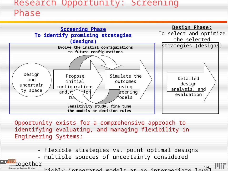
Research Opportunity: Screening Phase

Propose initial configurations and

decision rules

Simulate the outcomes using

screening models

Design and uncertainty

space

Detailed design analysis, and

evaluation

Screening PhaseTo identify promising strategies (designs)

Design Phase:To select and optimize the

selected strategies (designs)

Sensitivity study, fine tune the models or decision rules

Evolve the initial configurations to future configurations

Opportunity exists for a comprehensive approach to identifying evaluating, and managing flexibility in Engineering Systems:

- flexible strategies vs. point optimal designs- multiple sources of uncertainty considered together- highly-integrated models at an intermediate level of fidelity

11

Screening Approach as Augmentation of Current Practice

Level of detail

Level of integration

Low Mid

Alte

rnat

ives

Con

side

red

High

Low

High

few

man

y

Screening approach

Current practice(high-detailed domainmodels, point “optimal”solutions)

Computation time for each run

seconds Seconds ~ minutes

Hours ~ Days

Goal: Make sure the most promising strategies are

investigated during detailed design

12

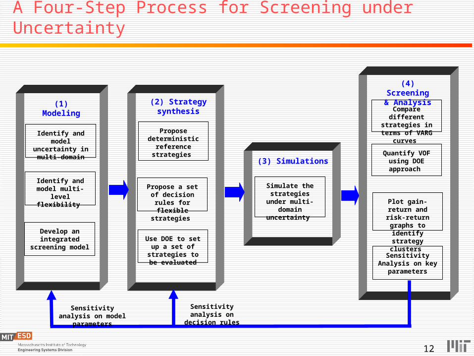
A Four-Step Process for Screening under Uncertainty

Identify and model uncertainty in multi-domain

Develop an integrated

screening model

Propose deterministic

reference strategies

Identify and model multi-level flexibility

Use DOE to set up a set of strategies

to be evaluated

Simulate the strategies under

multi-domain uncertainty

Propose a set of decision rules for flexible strategies

Sensitivity Analysis on key

parameters

Compare different strategies in terms of VARG curves

Quantify VOF using DOE approach

Plot gain-return and risk-return

graphs to identify strategy clusters

(1) Modeling (2) Strategy synthesis

(3) Simulations

(4) Screening& Analysis

Sensitivity analysis on decision rules

Sensitivity analysis on model parameters

13

Simulation Framework (step 3)

Monte Carlo Simulation i = 1:n1 (samples)

Simulation time step j = 1:n2 (years)

Decision Making Module

j > n2

Economic Outputs (e.g., NPV) for

sample i

i > n1

END

Outer Loop

Inner Loop

Uncertainty Learning Models

YES

YES

NO

NO

Endogenous Uncertainty

Model

Exogenous Uncertainty

Hybrid Uncertainty

Multi-domain uncertainty models

Resource systems

System designs

Integrated screening models

Project economics

Multi-level flexible strategies Strategic level Tactical level Operational level

Identified Strategies or Designs Probability distribution of outcomes:

Value-at Risk-Gain (VARG) curves Technical metrics: e.g., throughputs Economic metrics: e.g., NPV, CAPEX

Chapter 3

Chapter 4

Chapter 5

Case studies: Chapters 6&7

Chapter 3

Chapter 3

Strategies

Turn “on” or “off” flexibilities Strategic level: Y/N Tactical level: Y/N Operational level: Y/N

14

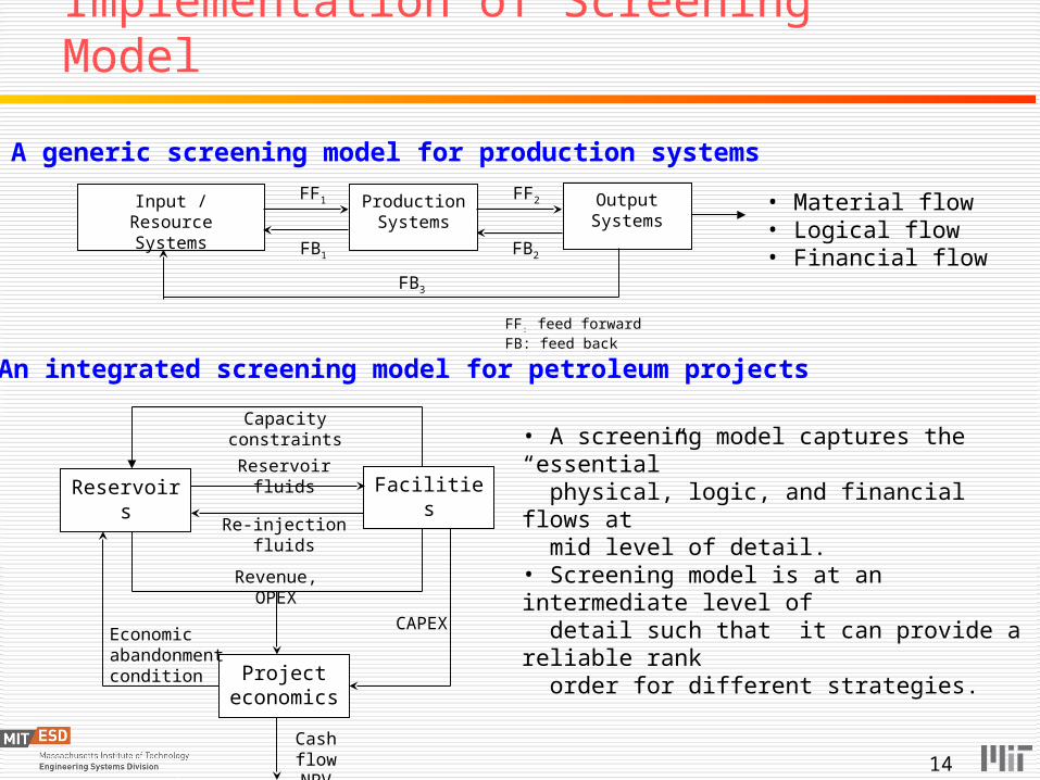
Implementation of Screening Model

A generic screening model for production systems

An integrated screening model for petroleum projects

• A screening model captures the “essential” physical, logic, and financial flows at mid level of detail.• Screening model is at an intermediate level of detail such that it can provide a reliable rank order for different strategies.

• Material flow• Logical flow• Financial flow

Input / Resource Systems

ProductionSystems

Output Systems

FF1 FF2

FB1 FB2

FB3

FF: feed forwardFB: feed back

Reservoirs Facilities

Project economics

Reservoir fluids

CAPEX

Re-injection fluids

Revenue, OPEX

Economic abandonment condition

Cash flowNPV

Capacity constraints

A Simulation Model for Reserve Evolution

05.02.03.015.02.015.0 000 P

tePtP 0

Random walk for P50 at each step

(2) Standard deviation (in log scale)

Probability of “disruptive changes”

Magnitude of “disruptive changes”

050 btP

Where Σ0 is initial standard deviation, “a” is a sample from standard normal distribution, “b” is a sample from uniform distribution [0.5 1.5]

0 5 10 15 20 25400

600

800

1000

1200

1400

1600Evolution of reservoir volume estimates (two realizations)

Number of Years

Res

ervo

ir V

olum

e (m

mst

b)

P50P50

P10

P10

P90P90

Example of disruptive change !

(1) Median (in log scale)

“Disruptive changes” of variation

Evolution of t

Assume reserve estimate follows lognormal distribution at any given point of time

ett 1

etct 1,max 0

Where “c” is a sample from uniform distribution [0.5 1]

tP eat 050

16

Application of the Screening Approach

Baseline NPV

NPV distribution

(RU+FU+MU)

NPV distribution

(RU + FU+ MU +

flexible facility)

NPV distribution

(RU + FU + MU +

flexible facility +

tieback)

Reservoir: reserve

+

+

Deterministic inputs:• Expected values for RU, FU, and MU • Optimize the designs of facilities

+

Flexible facilities+decision rules

RU: reservoir uncertaintyFU: facility uncertaintyMU: market uncertainty

Oil / gas price+

Traditional Traditional Practice:Practice:

Single number for NPV as decision Making criteria

New Approach: New Approach: Value-at-Risk-GainCurve (VARG)• Expected NPV• Maximal Gain• Maximal loss• Initial CAPEX• Value of Flexibility

0 2 4 6 8 10 12 14 16 18 200

10

20

30

40

50

60

70

80

90

100Facility Availability (FA)

Years of production

Faci

lity

Ava

ilabi

lity

(%)

FA

EFA

Facility Availability

0 2 4 6 8 10 12 14 16 18 200

10

20

30

40

50

60

70

80

90

100Facility Availability (FA)

Years of production

Faci

lity

Ava

ilabi

lity

(%)

FA

EFA

Facility Availability

0 2 4 6 8 10 12 14 16 18 200

10

20

30

40

50

60

70

80

90

100Facility Availability (FA)

Years of production

Faci

lity

Ava

ilabi

lity

(%)

FA

EFA

Facility Availability

“Bespoke”Design

+

+

Flexible facilities+ decision rules+ tie-back flexibility

+

Oil / gas price+

Oil / gas price+

(1)

(2)

(3)

(4)

Reservoir: reserve

Reservoir: reserve

Bespoke: point-optimal, customized

17

Problem “Landscape”

Case study 1:Compare four

field developmentstrategies

Case study 2:Tieback flexibility for small oilfields

Tie back options• FlexibilityA

C

BD

number of facility

Staged Development• Standardization• Flexibility

number of reservoir

1 2 3 4 51 12 13 14 15 1 16 17 1

Facility Index

Reservoir Index

Staged development of a large reservoir

Tie-back a small reservoir (ID 3)To facility ID 5 as capacity becomes available

e.g., fields in GoM, North Sea, Alaska Prudhoe Bay

e.g., ACG, Caspian sea, Azerbaijan

e.g., Angola B18 (Great Plutonio), B31

18

Multi-Level Flexibility in Oilfield Development

Multi-level flexibility:

•Strategic Level (inter-facility):Change the topological (architecture) of a network

• Tactical Level (intra-facility):Change the design/behavior of a node or connection

• Operational level:Change the flow rates

Facility

Field

Production flowline

Injection flowline Service lines

Stage 1

Stage 2

19

Outline Motivation Research questions and approach Literature review and gap analysis Integrated screening model approach:

A 4-step screening framework

A simulation process for screening under uncertainty (step 3)

Implementation of a screening model for offshore petroleum projects

Applications of the integrated screening model Case study 1: Staged development of a hypothetical large oil field

Case study 2: Tieback flexibility for deepwater small oilfields

Insights, contributions and future work

1) Single big stage development Single stage in year 0 with 100% capacity (180 MBD)

2) Pre-determined staged development Three identical stages (33% capacity each) in year 0, 2 and 4

90% learning factor on CAPEX and development / drilling time reduction

3) Flexible staged development Initial stage with 75% capacity

Future stage options: 33%, 50%, 75%, 100% capacity

Variable stages depending the evolution of reserve estimates

A decision rule determines when to add additional stage with how much capacity

Cost of flexibility: 10% of platform cost for the initial stage

4) Reactive staged development The initial stage is the same as strategy 1

Allow to add one additional stage with 100% capacity

Case Study 1: Development of a Large Oilfield

21

Simulation Results (RU only) Value-at-Risk-Gain (VARG) Curve

(with Reservoir Uncertainty(RU))

0

0.2

0.4

0.6

0.8

1

0 2 4 6 8 10Net Present Value [Billion $]

Cu

mm

ula

tive

Pro

bab

ility

Flexible staged Three stages One big stage Reactive staged

ENPV ENPV ENPV ENPV

One big stage

Pre-determinedthree-stages

Reactive staged

Flexible staged

DEVELOPMENTTYPE

NPV ($, Billions) CAPEX ($, Billions)

Expected Minimal MaximalStandard Deviation

Expected Total

Minimal Initial

Maximal Eventual

One big Stage 3.11 0.02 4.60 1.11 2.76 2.76 2.76

Three stages 2.81 0.03 4.10 0.97 3.12 1.14 3.12

Flexible staged 3.66 0.25 10.76 2.01 3.88 2.25 10.05

Reactive staged 3.40 0.02 7.93 1.62 3.15 2.76 5.52

22

Case study 1: Sensitivity Analysis Sensitivity to cost of option (flexible staged option)

Flexible staged

Reactivestaged

One big stage

Cost of option(% of initial 75% capacity

platform cost)0% 5% 10% 20% 30% 40% 50% 60%

Cost of option(% of the CAPEX for one big

stage)0.0% 1.5% 2.9% 5.9% 8.8% 12% 15% 18%

ENPV (Bn$) 3.75 3.70 3.66 3.57 3.47 3.38 3.29 3.19 3.40 3.11

Min NPV (Bn$) 0.34 0.30 0.25 0.17 0.08 0.00 -0.09 -0.18 0.02 0.02

Max NPV (Bn$) 10.85 10.80 10.76 10.66 10.52 10.47 10.37 10.27 7.93 4.60

Sensitivity to benefit of option (learning factor on CAPEX reduction)

Flexible stagedReactive staged

One big stage

Benefit of option 100% 95% 90% 85% 80%

ENPV (Bn$) 3.56 3.61 3.66 3.71 3.76 3.40 3.11

Min NPV (Bn$) 0.26 0.26 0.25 0.26 0.26 0.02 0.02

Max NPV (Bn$) 10.22 10.49 10.76 11.00 11.24 7.93 4.60

23

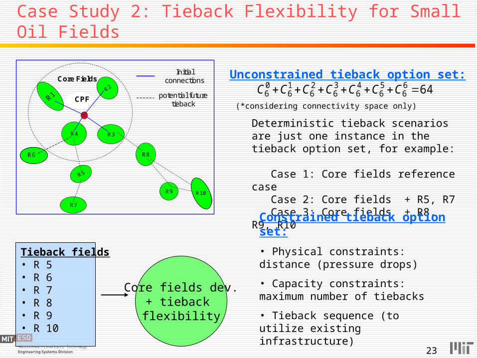
Case Study 2: Tieback Flexibility for Small Oil Fields

Core fields dev.+ tieback flexibility

Tieback fields• R 5• R 6• R 7• R 8• R 9• R 10

Unconstrained tieback option set:646

656

46

36

26

16

06 CCCCCCC

Deterministic tieback scenarios are just one instance in the tieback option set, for example: Case 1: Core fields reference case Case 2: Core fields + R5, R7 Case 3: Core fields + R8, R9, R10

Constrained tieback option set:

• Physical constraints: distance (pressure drops)

• Capacity constraints: maximum number of tiebacks

• Tieback sequence (to utilize existing infrastructure)

(*considering connectivity space only)

R4

R2

R3

R10

R8

R9

FPSO

R5

R7

R5

Core Fields

R6

R10

CPF

Initial connections

potential future tieback

24

Simulation Setup (with initial 150MBD)

Flexibilitytype

Strategic (inter-facility) flexibility

Tactical (intra-facility) flexibility

Operational flexibility

Strategy ID: Tieback flexibility:

X1 (Y/N)

Platform expansion flexibility

(150200 MBD): X2 (Y/N)

Active reservoir management:

X3 (Y/N)

Strategy 1 N N N

Strategy 2 N N Y

Strategy 3 N Y N

Strategy 4 N Y Y

Strategy 5 Y N N

Strategy 6 Y N Y

Strategy 7 Y Y N

Strategy 8 Y Y Y

*ARM: active reservoir management allows to temporarily shut down higher watercut fluids and allocates platform capacity to produce lower watercut fluids from tie-back reservoirs

Three factors and two levels’ full factorial design

25

Simulation Results (with Initial 150MBD, RU only)

Value-at-Risk-Gain curves are the cumulative probability distribution of projects’ outcomes, such as Net Present Value

Value-at-Risk-Gain (VARG) Curves(with Reservoir Uncertainty (RU))

0

0.2

0.4

0.6

0.8

1

-100 -50 0 50 100 150 200 250 300 350

Net Present Value [ % of ENPV of strategy 1]

Cu

mm

ula

tiv

e P

rob

ab

ility

Strategy 1 Strategy 2 Strategy 3 Strategy 4 Strategy 5 Strategy 6

Strategy 7 Strategy 8 ENPV_1 ENPV_2 ENPV_3 ENPV_4

ENPV_5 ENPV_6 ENPV_7 ENPV_8

Strategies 1&2

Strategies 3&4

Strategy 5

Strategy 7

Strategy 6

Strategy 8

26

*Initial CAPEX is defined as the CAPEX occurs before the first oil (within the first three years of development)

Expected Min Max σ(NPV) Expected Min Max Initial*Strategy 1 100 -66 251 74 100 100 100 64 100 0.0Strategy 2 100 -66 255 74 100 100 100 64 100 0.0Strategy 3 94 -88 262 77 102 100 109 64 100 0.0Strategy 4 94 -88 260 77 102 100 109 64 100 0.0Strategy 5 132 7 266 54 138 104 172 66 148 2.5Strategy 6 152 27 276 50 138 104 172 66 148 2.5Strategy 7 147 22 281 47 177 137 204 66 183 5.2Strategy 8 177 22 335 61 177 137 204 66 183 5.2

Expected total reserve

Expected # of tiebacks

NPV (% of ENPV for strategy 1 )CAPEX (% of exptected CAPEX for

strategy 1)

323121321321 25.125.65.625.65.35.275.124,, xxxxxxxxxxxxENPV

0

10

20

30

40

50

60

Co

ntr

ibu

tio

n t

o E

NP

V

(% o

f E

NP

V o

f S

tra

teg

y 1

)

x1 x1x2 x3 x1x3 x2 x2x3

Main Effects or Interaction Effect

Pareto Chart for Main Effects and Interaction EffectsTieback

flexibilityOperationalflexibility

Simulation Results (with initial 150MBD, RU only)

Value of Flexibility (VOF)= ENPV (w flexibility) -ENPV (w/o flexibility)

27

Strategy Clusters (mean-variance plot)

• Cluster 1: strategies with lowest return and highest variance (1,2,3,4,9,10)• Cluster 2: strategies with mid-range return and the lowest variance (5,6,7,11)• Cluster 3: strategies with highest return and mid-range variance (8,12)

Blue line looks likea “mean-variance efficient frontier” in Capital Asset Pricing Model (CAPM)“the set of mean-variance choices from the Investment opportunity set where for a given variance no otherInvestment opportunity offers a higher mean return”

ENPV vs. standard deviation of NPV

-50

0

50

100

150

200

250

40 45 50 55 60 65 70 75 80

Normalized standard deviation of NPV ( % of ENPV for strategy 1 )

No

rmal

ized

EN

PV

(%

of

EN

PV

fo

r st

rate

gy

1)

Cluster 2(with tiebackwith cpacity or ARM flex )

Cluster 1(no tieback)

Cluster 3(Full flex)

Strategy 8Strategy 12

Strategy 6

P10

P90

Strategy 1&2

Efficient Frontier

Key Insights Flexible Strategies can create significant additional value

Increase in ENPV (expected value) compared to a rigid baseline case Case 1: ENPV of $3.66B (flexible staged deployment) vs. $3.11B (single stage) Case 2: ENPV of strategy 8 (Y/Y/Y) is 177% of strategy 1 (100% baseline)

Impact of flexibility can be largest when looking at tails, not the mean Enhancing upside opportunity: Case 1: max(NPV) $10.76 vs. $3.11B (single stage) Minimizing downside risk: Case 2: -66% for strategy 1 vs. +22% for strategy 8

Interaction amongst various types of flexibility Strategic level flexibility creates most value

Case 2: tie-back flexibility created 50-60% extra NPV

Operational flexibility can enhance value created by strategic options Case 2: Active Reservoir Management (ARM) contributes 10-15% extra NPV Some options don’t have value unless other types of flexibility are also present

Role of uncertainty Sources of uncertainty affect engineering systems in different ways

Reservoir uncertainty shifts distributions horizontally Facility uncertainty (availability) affects all strategies equally by lowering NPV Market uncertainty tends to extend tails and dilute differences between strategies

Fidelity of results Rank order of strategies tends to be robust

Case 1 Sensitivity analysis: Cost of staged deployment flexibility can be as high as 40% of initial platform CAPEX and flexibility strategy still wins over the base case

28

29

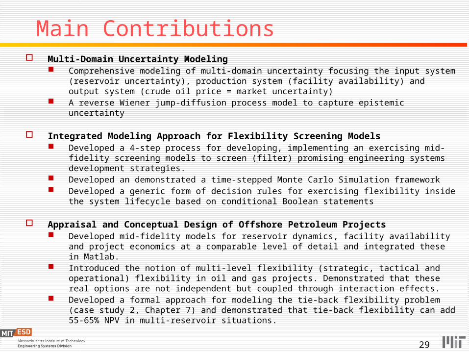
Main Contributions Multi-Domain Uncertainty Modeling

Comprehensive modeling of multi-domain uncertainty focusing the input system (reservoir uncertainty), production system (facility availability) and output system (crude oil price = market uncertainty)

A reverse Wiener jump-diffusion process model to capture epistemic uncertainty

Integrated Modeling Approach for Flexibility Screening Models Developed a 4-step process for developing, implementing an exercising mid-

fidelity screening models to screen (filter) promising engineering systems development strategies.

Developed an demonstrated a time-stepped Monte Carlo Simulation framework Developed a generic form of decision rules for exercising flexibility inside the

system lifecycle based on conditional Boolean statements

Appraisal and Conceptual Design of Offshore Petroleum Projects Developed mid-fidelity models for reservoir dynamics, facility availability and

project economics at a comparable level of detail and integrated these in Matlab. Introduced the notion of multi-level flexibility (strategic, tactical and operational)

flexibility in oil and gas projects. Demonstrated that these real options are not independent but coupled through interaction effects.

Developed a formal approach for modeling the tie-back flexibility problem (case study 2, Chapter 7) and demonstrated that tie-back flexibility can add 55-65% NPV in multi-reservoir situations.

30

Vision: Learning in Engineering Systems

Sensor Decision rules Exercise optionsLearning

Screeningstrategies using

the integrated model

Collect Informationi.e., exploration wells, market conditions, and demands

Process informationi.e., estimate reserves(iterative process, i.e., Bayesian learning)

Trigger decision rulesi.e., if Δreserve (t) > aAND crude oil price(t) > bTHEN do this

Exercise catalogue of options i.e., add 2nd 30% or 50%capacity flexibility, tieback flexibility

Technical and economic outcomesi.e., reservoir production profiles, NPV, VARG

Develop anintegrated

model

Capture resource systems, technical designs, and economics, and their interactions at mid-detailed level

This framework providesdecision makers a “computational lab” to efficiently experiment a large number of possible scenarios before deciding on a specific plan!

31

Future work

Quantify the levels of model-fidelity (MFL similar to TRL?)

Comprehensive catalogue of real options (flexibility) such as reserving margins, extra interfaces, enable multiple paths …

Improve reservoir uncertainty models: estimate model parameters from historical data, Bayesian learning framework

Improve decision rules: sensitivity analysis, obtain experts’ implicit knowledge, adaptive (self-tuning) decision rules

Use low fidelity models (e.g., architecture generators such as OPN) to generate more promising development scenarios to be evaluated by screening models

Integrate with multi-stakeholder analysis and model other non-monetary flows (such as emissions, jobs …), include contractual barriers and enablers in multi-stakeholder contexts

Thank you!