EXPLORATION OF THE PHASE FIELD FRAMEWORK MARMOT TO INCLUDE

EXPLORATION OF THE PHASE FIELD FRAMEWORK MARMOT TO INCLUDE

ANISOTROPIC GRAIN BOUNDARIES WITH MOLECULAR DYNAMICS

by

Aaron S. Butterfield

A senior thesis submitted to the faculty of

Brigham Young University - Idaho

in partial fulfillment of the requirements for the degree of

Bachelor of Science

Department of Physics

Brigham Young University - Idaho

July 2013

Copyright c© 2013 Aaron S. Butterfield

All Rights Reserved

BRIGHAM YOUNG UNIVERSITY - IDAHO

DEPARTMENT APPROVAL

of a senior thesis submitted by


This thesis has been reviewed by the research committee, senior thesis coor-dinator, and department chair and has been found to be satisfactory.

Date Richard Datwyler, Advisor

Date Evan Hansen, Senior Thesis Coordinator

Date Kevin Kelley, Committee Member

Date Stephen Turcotte, Chair

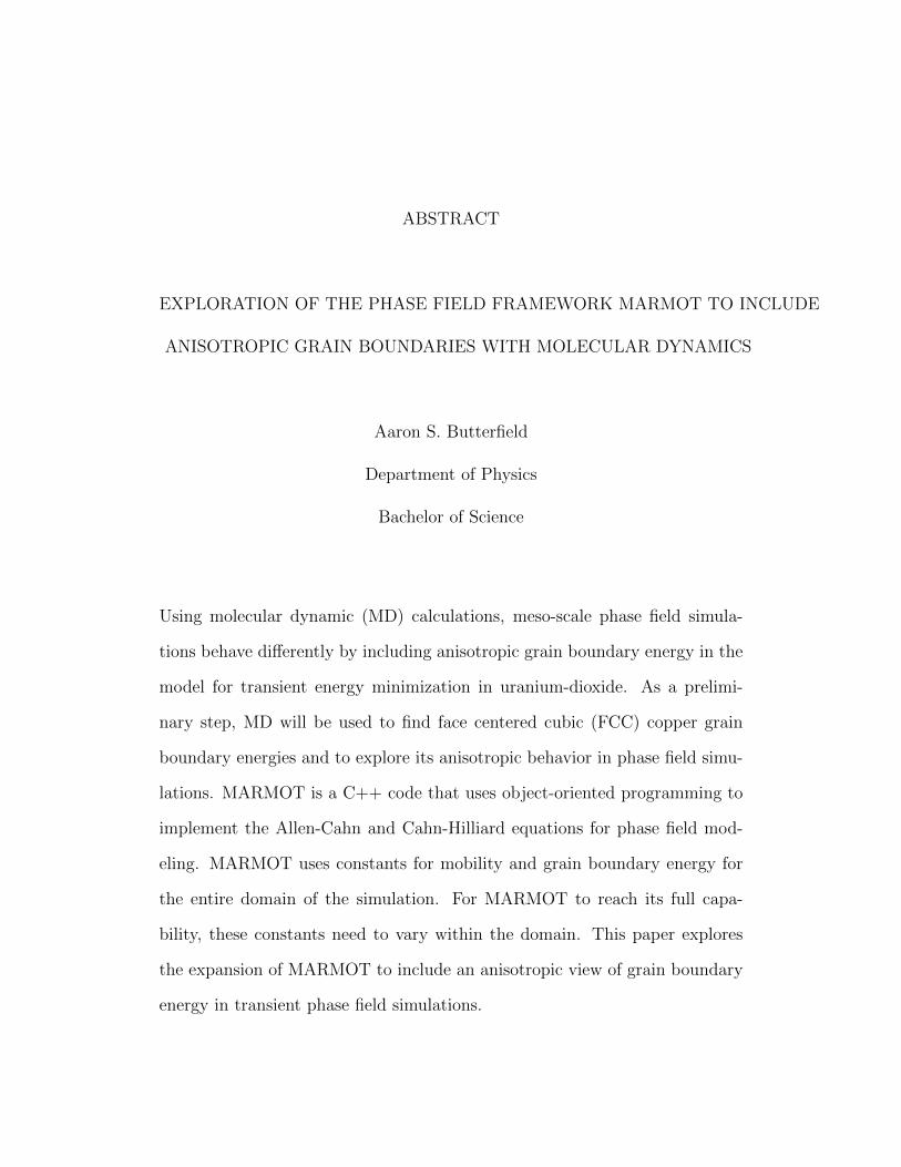
ABSTRACT

EXPLORATION OF THE PHASE FIELD FRAMEWORK MARMOT TO INCLUDE

ANISOTROPIC GRAIN BOUNDARIES WITH MOLECULAR DYNAMICS


Department of Physics

Bachelor of Science

Using molecular dynamic (MD) calculations, meso-scale phase field simula-

tions behave differently by including anisotropic grain boundary energy in the

model for transient energy minimization in uranium-dioxide. As a prelimi-

nary step, MD will be used to find face centered cubic (FCC) copper grain

boundary energies and to explore its anisotropic behavior in phase field simu-

lations. MARMOT is a C++ code that uses object-oriented programming to

implement the Allen-Cahn and Cahn-Hilliard equations for phase field mod-

eling. MARMOT uses constants for mobility and grain boundary energy for

the entire domain of the simulation. For MARMOT to reach its full capa-

bility, these constants need to vary within the domain. This paper explores

the expansion of MARMOT to include an anisotropic view of grain boundary

energy in transient phase field simulations.

ACKNOWLEDGMENTS

In the pursuit of my bachelors degree there are many people that I would

like to thank and praise for helping me get where I am today. I would like to

first thank my wife, Becca, for all of her support, patience, faith, prayers and

love in my endeavor to obtain my degree. My parents have always believed

in my ability to accomplish great things and provided lifetime of support and

love. I thank Idaho National Laboratories (INL) for allowing me to use their

High Performance Computing supercomputers and for the financial contribu-

tion of INL and the Department of Energy to my research. I appreciate Dr.

Michael Tonks and Dr. Yongfeng Zhang for their advice and aid in my re-

search. Kip Harris, Dean of Students at Brigham Young University Idaho,

allowed me access to INLs supercomputing clusters from campus. Thank you

to Dr. Richard Datwyler, Dr. Kevin Kelley, and Dr. Evan Hansen in the BYU

Idaho physics department for their valuable comments and advice.

Contents

Table of Contents xi

List of Figures xiii

1 Introduction 11.1 Nuclear Power in the Future . . . . . . . . . . . . . . . . . . . . . . . 11.2 Light Water Reactor Sustainability . . . . . . . . . . . . . . . . . . . 21.3 Modeling in the Future . . . . . . . . . . . . . . . . . . . . . . . . . . 21.4 Grain Boundaries in Material Science . . . . . . . . . . . . . . . . . . 5

2 Theory and Methods 72.1 Theory . . . . . . . . . . . . . . . . . . . . . . . . . . . . . . . . . . . 8

2.1.1 Molecular Dynamics . . . . . . . . . . . . . . . . . . . . . . . 82.1.2 Finite Element Method . . . . . . . . . . . . . . . . . . . . . . 102.1.3 Phase Field Modeling . . . . . . . . . . . . . . . . . . . . . . . 11

2.2 Methods . . . . . . . . . . . . . . . . . . . . . . . . . . . . . . . . . . 132.2.1 Molecular Dynamics Method . . . . . . . . . . . . . . . . . . . 132.2.2 Anisotropic Model in MOOSE and MARMOT . . . . . . . . . 14

3 Results 193.1 Grain Boundary Energies . . . . . . . . . . . . . . . . . . . . . . . . . 193.2 Verifying the Data . . . . . . . . . . . . . . . . . . . . . . . . . . . . 203.3 Using the Data in the Phase Field Simulation . . . . . . . . . . . . . 22

4 Summary and Conclusions 254.1 Validate Values Obtained from MD . . . . . . . . . . . . . . . . . . . 25

Bibliography 27

Bibliography 27

A Code 29A.1 LAMMPS . . . . . . . . . . . . . . . . . . . . . . . . . . . . . . . . . 29A.2 C++ . . . . . . . . . . . . . . . . . . . . . . . . . . . . . . . . . . . . 31

xi

List of Figures

1.1 Uranium Oxide Fuel Pellets . . . . . . . . . . . . . . . . . . . . . 31.2 Uranium Oxide Fuel Cracking and Fatigue . . . . . . . . . . . 41.3 Grain Structure of Material . . . . . . . . . . . . . . . . . . . . . 5

2.1 Simplifying Complex Geometric Shapes . . . . . . . . . . . . . 102.2 MOOSE Block Diagram . . . . . . . . . . . . . . . . . . . . . . . 152.3 Anisotropic Model for MARMOT . . . . . . . . . . . . . . . . . 17

3.1 Results of Two Molecular Dynamics Simulations . . . . . . . . 203.2 Grain Boundary Energies by Orientation . . . . . . . . . . . . . 213.3 Post Processor View of Kappa Across the Domain . . . . . . 23

xiii

Chapter 1

Introduction

1.1 Nuclear Power in the Future

The United States led the way in the early development of nuclear energy. As the DOE

looks toward the future, it is apparent that nuclear energy has a significant place in the

United States’ energy security; however, today’s world is a much different place than

in the mid 1900’s. After the terrorist attacks in New York City and Washington DC,

nuclear non-proliferation is of paramount concern. The recent accident in Fukoshima,

Japan and past accidents at Three Mile Island and Chernobyl create questions about

the safety of existing nuclear reactors. Amid these challenges, the world has a growing

need for energy and it is only going to increase in the coming years. “Domestic demand

for electrical energy is expected to grow by more than 20% from 2011 to 2040.”[1]

As a result, the Department of Energy (DOE) is very interested in cost-effective,

environmentally friendly, safe, and sustainable energy sources, particularly nuclear

energy.

1

2 Chapter 1 Introduction

1.2 Light Water Reactor Sustainability

The DOE is taking a two-pronged approach to nuclear research. They are working

on maintaining and revitalizing their existing fleet of Light Water Reactors (LWRs)

and designing next-generation nuclear reactors. Many of the existing reactors contain

outdated sensors and control systems that need to be replaced to make them safer

and more automated. Due to the harsh conditions inside a reactor, the state of

the components (walls, cladding, coolant pipes, etc.) deteriorates and the reactor

becomes costly to re-certify. In an effort to maintain and revitalize the existing

LWRs, the DOE is funding research for computational models that are accurate

enough to target the deteriorating components to replace for re-certification and to

find innovative ways to make the reactors more efficient. “The Light Water Reactor

Sustainability Program is developing the scientific basis to extend existing nuclear

power plant operating life beyond the current 60-year licensing period and ensure

long-term reliability, productivity, safety, and security.”[1] This will allow the current

LWRs to operate while research is being done to develop the next generation reactors.

[1]

1.3 Modeling in the Future

Computational modeling maximizes the important results gained from experiments.

Computational modeling and experimental methods have their strengths and weak-

nesses, but if used together, their weaknesses are minimized and their strengths are

maximized. Building large scale experiments are more expensive than using computa-

tional methods; however, computational methods are only as correct as their model.

As a result, computational modeling can be used to guide costly experiments to look

for specific data that would be of the most worth. Experiments performed in test

1.3 Modeling in the Future 3

Figure 1.1 Uranium Oxide Fuel Pellets

reactors can take years to run. This extended time scale causes the data from the

experiment to be gathered at a trickle compared to running simulations in a cluster or

supercomputer. The data gathering is further prolonged if other preliminary experi-

ments need to be preformed. Computational modeling has the ability to run some of

the preliminary experiments numerically first. Often, scientists will use a “bake and

check” method, where a material left in a reactor is cut open and the grain structure

is analyzed to make inferences about what occurred on the meso-scale during its time

in the reactor. These inferences can be supported by computational simulations that

check if our understanding is correct.

The current models used for nuclear engineering for LWR design need to be

adapted for next generation designs. Computational models will simulate next gen-

eration reactors to anticipate specific design adaptations. For example, the High

Temperature Gas-Cooled Reactor (HTGR) uses a compressible fluid instead of an

incompressible fluid as its coolant. “HTGRs are intrinsically different from conven-

tional. . . LWRs, which leads to issues in adapting traditional numerical methodologies.

For example, a large temperature difference between the reactor inlet and outlet cre-

ates a significant density variation in the helium coolant. In this case, employing


Figure 1.2 Uranium Oxide Fuel Cracking and Fatigue

an incompressible assumption and using the Boussinesq approximation for buoyancy

may not give accurate heat transfer results.”[2] Currently there are no next generation

reactors, so computational methods will be heavily relied on as they are built.

As the cost of computing has decreased over the years, it has allowed computa-

tional research, particularly in LWRs, to reach a new level for existing technologies.

“Modeling and simulation has a long history with researchers and scientists exploring

nuclear energy technologies. In fact, the existing fleet of currently operating reac-

tors was licensed with computational tools that were produced or initiated in the

1970s. Researchers and scientists in Nuclear Energy Advanced Modeling and Simu-

lation (NEAMS) are developing new tools to predict the performance, reliability and

economics of advanced nuclear power plants. The new computational tools will allow

researchers to explore in ways never before practical, at the level of detail dictated

by the governing phenomena, all the way from important changes in the materials of

a nuclear fuel pellet to the full-scale operation of a complete nuclear power plant.”[1]

As nuclear research moves forward, both computational modeling and experimen-

tal methods will be vital in engineering and researching current and future designs.

1.4 Grain Boundaries in Material Science 5

Figure 1.3 Grain Structure of Material

1.4 Grain Boundaries in Material Science

Grain sizes in materials affect the overall properties of the material. Often engineers

will assume that the properties in a material is the same in every direction (isotropic),

however, the properties of many materials vary based on the direction or orientation

(anisotropic).

Because of the extreme conditions inside a nuclear reactor, understanding grain

structure at the meso-scale is imperative. For example, temperature gradients across

fuel pellets can change over a one-thousand degrees kelvin in a centimeter. Grain sizes

greatly affect the thermal conductivity and thereby become an important attribute to

understand for efficient and safe coolant flows. Not only have these effects been seen

in models, but they have now been verified experimentally by looking at the spent

cladding of nuclear reactors.


Chapter 2

Theory and Methods

The use of computational methods allows researchers to know how a reactor will

behave from an engineering perspective. At Idaho National Laboratories (INL), com-

putational modeling is leading the way for experiential research. They have developed

two applications called MOOSE (Multi-Physics Object Oriented Simulation Environ-

ment) and MARMOT. MOOSE is an object oriented code that employs the finite

element method (FEM) for nuclear research and design. MARMOT is an extension

of MOOSE that allows for simulation of phase field models. In the current models

that MOOSE and MARMOT employ, MARMOT assumes that the grain boundary

energy across each grain boundary is only a factor of its area and not its orientation,

relative to the adjacent grain. In reality, materials have several different kinds of

grain boundaries; each differs in its energy per area due to its grain orientation with

the adjacent grain. Changing the framework to include these cases will allow a more

realistic view of materials at the meso-scale.[3]

Understanding how fuel pellets behave under the extreme conditions inside a nu-

clear reactor is central to the designing of safer, economical, and environmentally

friendly reactors. Uranium dioxide fuel pellets power most of the reactors today. I

7

8 Chapter 2 Theory and Methods

have chosen to use FCC copper for preliminary research to validate an anisotropic

model that can be employed in the future to analyze the grain structure of uranium

dioxide. There is a vast amount of data about FCC copper available in the research

community to validate my findings and its simple lattice structure makes the molec-

ular dynamics easier to implement.

2.1 Theory

In my research, I will be using three areas of computational science to build an

anisotropic model of FCC copper:

1. Molecular Dynamics

2. The Finite Element Method

3. Phase Field Method

2.1.1 Molecular Dynamics

Molecular dynamics (MD) uses Newton’s second law to calculate the positions and

velocities of a system of particles. Given the initial conditions of the system, many of

its thermodynamic properties can be obtained. MD can be used for any multi-body

system; however, it tends to be used for the study the motion of molecules, hence,

the name ”molecular dynamics.”[4]

LAMMPS (Large-scale Atomic/Molecular Massively Parallel Simulator) is an MD

software package produced by Sandia National Laboratories. It uses the embedded

atom method (EAM) to calculate position, acceleration, pressure, and energy. The

EAM is represented by equation 2.1,

2.1 Theory 9

Ei = Fα

∑i 6=j

ρβ(rij)

+1

2

∑i 6=j

φαβ(rij), (2.1)

where rij represents the distance between atoms i and j. ρβ represents the contri-

bution of atom j, of type β, on the electron gas cloud. Fα is the embedded energy

function representing the amount of energy necessary to embed an atom i, of type α,

within the electron gas cloud. φij is a function that represents the pairwise interaction

of the atoms i and j.

Because MD simulations calculate energy and forces of a given system, energy

minimization through various methods is possible. LAMMPS has an energy mini-

mization operating mode which translates atoms randomly to find a minimum energy

state within the configuration. LAMMPS also allows you to minimize the system

while holding some thermodynamics properties constant, such as volume, entropy,

enthalpy, etc. The lowest energy can be achieved by using a series of minimizations

with different thermodynamic properties.

Grain boundary energies are found by subtracting two minimized system energies.

A monocrystalline material represents the lowest energy state possible. LAMMPS

keeps a running total of the energy of the system as it minimizes. After obtaining

the result for the monocrystalline (EMONO) and polycrystalline (EPOLY ) materials,

the grain boundary energy, (EGB), can be achieved by finding the difference between

the two systems energies and dividing the energy by twice the area (A) of the grain

boundary.

EGB =EPOLY − EMONO

2A(2.2)


2.1.2 Finite Element Method

The Finite Element Method (FEM) is “a numerical analysis technique for obtaining

approximate solutions to a wide variety of engineering problems...the basic premise

of the finite element method is that a solution region can be analytically modeled or

approximated by replacing it with an assemblage of discrete elements.”[5]

Figure 2.1 Simplifying Com-plex Geometric Shapes

Most people get exposed to the fundamentals

of FEM in their first geometry class. You see

a complex shape when you look at the following

shape in figure 2.1. When asked to find the area

of the shape, almost without thinking, you sepa-

rate or discretize the domain into smaller pieces

to simplify the problem. In FEM we separate

a complex shape into smaller, more manageable,

elements that the computer can easily handle.

Several numerical analysis methods have been

developed over the years. One common model is

the finite difference method; it uses a grid point

system to discretize its domain, which means that

information is only available for those points and

the rest of your domain is left without data. This

method is difficult to use for irregular geometries

and unusual boundary conditions. A benefit of

using FEM is that it is meant for complex shapes

and you can have continuous data over your whole domain. [5]

In nuclear engineering, a continuous domain is important to maintain while looking

at very complex shapes. For example, a nuclear reactor has several fuel rods that are

2.1 Theory 11

bathed in a pool of water. The fuel rods of a reactor also have control rods that

slide over the them to control the nuclear reaction that generates the heat. The

location of the control rods on the fuel rods greatly influence the performance of the

reactor. Modeling the reactor using complex geometry is essential to understanding

how quickly the water can remove the heat from the reactor.

2.1.3 Phase Field Modeling

The phase field method uses the FEM to analyze the behavior of interfaces between

different materials (eg. oil and water) or phases of the same material (eg. ice and wa-

ter). The model uses the Allen-Cahn and Cahn-Hilliard equations to track interfaces

between different phases or materials as they evolve over time. Within the phase

field framework, each phase or material is represented by “continuous variables that

smoothly transition from one value to another...this description of the interfaces elim-

inates the need to explicitly discretize a[n]...interface.” [3] These continuous variables

represent the existence of a phase or material at a given point.

A one-dimensional example is the step function in mathematics. Consider the

function f(x) = x2; in order to make the function to exist between the values of

2 < x < 3, we can utilize a step function. The step function is defined as 2.3

u(x) =

0 x < 0

1 x ≥ 0, (2.3)

using this function we can represent our variable as equation 2.4,

φ(x) = f(x) ∗ (u(x− 2)− u(x− 3)), (2.4)

where φ is the order parameter. The order parameter is defined over the entire domain,

but, f(x) is only between 2 < x < 3. In the phase field approach, micro-structural


features are described using continuous variables. These variables take two forms:

conserved variables representing physical properties such as atom concentration or

material density, and non-conserved order parameters describing the microstructure

of the material, including grains and different phases.[3]

The evolution of these order parameters is a function of the derivative of the Gibbs

free energy, which in turn is a function of the order parameters. The time evolution

of the conserved order parameters proceeds according to the Cahn-Hilliard partial

differential equation (PDE) 2.5,

∂ci∂t

= ∇ ·Mi∇∂F

∂ci, (2.5)

where ci is the conserved order parameter, Mi is the associated mobility, and F is

the free energy functional. The time evolution of the non-conserved order parameters

proceed according to the Allen-Cahn PDE 2.6,

∂ηj∂t

= −Lj∂F

∂ηj, (2.6)

where ηi is the non-conserved order parameter and Lj is the non-conserved order

parameter mobility. For a system using N conserved order parameters and M non-

conserved order parameters, the free energy functional follows the form

F =∫V

[floc(ci, . . . , cN , ηi, . . . , ηM) + fgr(ci, . . . , cN , ηi, . . . , ηM) + Ed], (2.7)

where floc is the local free energy and fgr is the gradient free energy, and Ed is

any long distance energy provided by electromagnetic or pressure applied from the

outside of the material.

For the cases of grain boundary motion equation 2.8 represents the floc,

floc = µ(η3i − ηi + 2N∑j 6=1

ηiη2j ), (2.8)

2.2 Methods 13

where µ represents a model parameter that is related to the grain boundary surface

energy. The fgr is defined as

fgr =N∑i

κi/2|∇ci|2 +M∑i

κj/2|∇ηj|2, (2.9)

for all of the conserved and non-conserved order parameters. In MARMOT, the phase

field model assumes that µ,κi, κj, Mi, and Lj are constants. This is what we will

call the isotropic case. In reality, grain boundaries have different energies based on

their orientation with adjacent grains. This is the called the anisotropic case. My

anisotropic model continues to treat the order parameter mobilities (Mi and Lj) as a

constants, but will allow µ, κi, and κj to vary throughout the domain.

2.2 Methods

Now that the numerical method’s theory has been explained, we need to understand

how it is applied. I will outline the MD procedure for calculating grain boundary

energies and how that data will be used to implement anisotropic behavior in MAR-

MOT.

2.2.1 Molecular Dynamics Method

In the LAMMPS input file I set the units in which I wanted the simulation to be

performed. In this case, the unit’s setting name is called “metal.” The distance will

be in angstroms, mass is in amu, time is in picoseconds, energy is in eV, etc. The

lattice is set to a unit length of 3.61070A with an orientation of x along [100]. I

created a simulation box of 50 x 50 x 50 A and split it into two regions, one for

the top grain and one for the bottom. In the monocrystalline structure, the top and

bottom regions have the same lattice. The monocrystalline structure is the minimum


energy state in which all the other simulations will be compared. Then I imported

the EAM file which contains the potential for copper and specified a cut-off distance

for the potential. The temperature for all the simulations was set to 0K. Then I

minimized the system twice, once fixing the volume as a constant, and once, allowing

the volume to change in the z direction. After each minimization, I calculated the

grain boundary energy from equation 2.2.

After calculating the minimum energy for the monocrystalline structure, I found

the minimum energy for several orientations of polycrystalline structures. My orien-

tation of the bottom grain was based on φ and θ of a spherical coordinate system. In

order to use angles from a spherical coordinate system, I had to define a FCC copper

unit cell in a custom way. I used a python script to loop through φ and θ from 0 to

π/2 to batch-process each MD simulation.

2.2.2 Anisotropic Model in MOOSE and MARMOT

MOOSE is a compilation of other powerful software which provides rich framework to

build our new anisotropic model by modularizing its code into classes. The modules

and pieces of MOOSE are listed on figure 2.2.

In order to understand the new anisotropic model of grain boundaries, it will be

important to understand four of the classes or modules in MOOSE and what they do.

The four classes are Kernels, Materials, Boundary Conditions, and Initial Conditions.

Kernels

Kernels describe the physics in the simulation and they contain PDEs that have

been reduced to their weak form. Higher-order equations are reduced by using the

divergence theorem. Because of MOOSE’s object oriented roots, scientists and engi-

neers can focus on the PDEs and not on monotonous programing syntax. Instead,

2.2 Methods 15

Figure 2.2 MOOSE Block Diagram

the PDEs can almost be added to the simulation exactly in its weak form. In the

anisotropic model, the kernel that we will use is found in equation below. As we

apply the divergence theorem and reduce the equation to its weak form, it looks like

this:

(∂ηj∂t, φm) = −L(κj∇ηj,∇φm)−L(

∂floc∂η

+∂Ed∂η

,∇φm)+L < κj∇ηj·~n,∇φm > . (2.10)

The last term of the equation represents our boundary condition and the other parts

represent the differential equation that includes the physics in our domain. MARMOT

uses equation 2.10 as superclass that all other subclasses are based upon. MOOSE is

open to any PDE under the sun; however, MARMOT limits itself to just the phase

field perspective. As a result, the only functions that need to be provided are ∂floc∂η

and ∂Ed

∂η. MARMOT simplifies the use of MOOSE for phase field simulations using

the Allen-Cahn equation. For the purpose of grain boundaries, ∂floc∂η

is the derivative

of equation 2.8.


Materials

Notice in the equations 2.5, 2.6, 2.8, and 2.9, there are several coefficients which are

not provided in the kernel. These coefficients are calculated at each quadrature point.

In FEM, an integral is taken to drive the residual to zero. Each node of the elements

carries the value of the order parameter η. A test function is used to multiply by and

an integral is taken to perform a best fit to the domain. MOOSE uses Newtonian

Quadrature to integrate over the domain. As a result, the error on integration is zero

due to every test function being a polynomial.

At every quadrature point throughout the domain, the kernel class calls the ma-

terial class. The material class calls the computeQpProperties() function, which con-

tains whatever code the user would like to run to provide the coefficients at each

quadrature point.

Boundary and Initial Conditions

Boundary conditions (BCs) and initial conditions (ICs) are very intuitive; however, it

is important to understand what MOOSE has built into it. MOOSE uses Dirichlet,

Neumann, and periodic BCs. For the most part in our simulations at the meso-scale,

we use periodic BCs which are already included and do not have to be programed.

ICs are set by overloading a function called value() in the IC‘s superclass. The

input to the function is a point data type which represents arbitrary points in the

domain. Using conditional statements, an individual provides the initial conditions

for the transient simulation.

The Model

The new model exists as a material class in the MOOSE framework, and is called

AnisotropicGrainBoundaryEnergy. This class will inherit all of the properties of the

2.2 Methods 17

Figure 2.3 Anisotropic Model for MARMOT


material class. It then overloads the computeQpProperties() function. As the object

of the class is created at the beginning of the simulation, the MD database of grain

boundary energies is loaded into a multidimensional array for easy reference by the

constructor of the class. Further, the constructor will couple each of the order pa-

rameters into the simulation to reference where the quadrature point is within the

domain and how close the point exists to each of the grains. The model will allow

the user to define the orientation of the grains in the simulation or let the user assign

a random distribution to each grain.

As the simulation starts, quadrature points will be evaluated. As the compute-

QpProperties function is called, the function checks the quadrature points location

to the nearest grains and uses one of the grains as a reference orientation. Then the

function calculates the difference between the two orientations according to φ and θ.

Referencing the container of energies, it finds the closest energy to the calculated φ

and θ.

Chapter 3

Results

3.1 Grain Boundary Energies

Minimizing the MD lattices took a large portion of time. The simulations used over

4,500 CPU-hours. I used a program to create many folders for each simulation that

needed to be run. I started the run, saving all of the trajectory information of the

atoms in each simulation. Once it filled up over 800 GB of data, I had to stop

collecting that data. After running the simulation, I compared the minimized single

crystalline lattice to the other polycrystalline lattices and found that the simulation

allowed other lattices to minimize lower in energy than what should be the base

energy. I believe this happened because I did not delete as many atoms as I should

have, allowing some atoms to be too close together. Also, the atoms were placed in

each region separately which resulted in the lattice restarting its pattern rather than

just filling the whole simulation box with one lattice command. This would have

eliminated the need for deleting atoms. To correct this, I found the lowest energy of

the calculated grains and made that the zero reference point, and the grain boundary

energies were plotted according to φ and θ. The results of the grain boundary energies

19

20 Chapter 3 Results

(a) Monocrystalline Lattice (b) Polycrystilline Lattice

Figure 3.1 Results of Two Molecular Dynamics Simulations

are located in figure 3.2. The energies followed a general trend, increasing in energy

as the angle increased further away from a monocrystalline structure. The graph

shows grain boundary energies as a function of φ and θ. The grain boundaries form

an interpolated surface and the grain boundary energies follow a general trend with

a few exceptions of spikes in the data.

3.2 Verifying the Data

Though numerical modeling is an estimate of the real world, we must get it as close as

we can to the real values for the model to be accurate. MARMOT has used 0.708J/m2

for the grain boundary energy everywhere, as stated in a paper by Schonfelder[6]. It

is the value of a 30 degree twist boundary. I compared my 30 degree twist boundary

energy with his to see that mine was and found that both were very comparable.

3.2 Verifying the Data 21

Figure 3.2 Grain Boundary Energies by Orientation


3.3 Using the Data in the Phase Field Simulation

Once I obtained the energies for different orientations, it was time to apply them to the

anisotropic model. Using the code that can be found in Appendix A, I used the grain

boundary energies to calculate the constants µ and κ in the material model. Running

the simulation I was able to watch κ, and κ and µ were doing exactly what I wanted.

They were being defined on the grain boundaries and were zero everywhere else. It

was fine that it was zero everywhere else; however, I could not get the simulation to

converge. This showed that µ and κ could not still be treated as constants and had to

be defined as functions of the order parameters. This added a larger complexity to the

problem many were hoping was negligible. As you can see by the figure, my material

property worked well for the assumption that I was trying to make. In the figure it

shows a pixilated nature for κ. This is not an accurate representation of the data.

Instead, they were actually defined at each quadrature point; but, the post-processor

in elemental so it averages the values of the quadrature points and reports one value

for each element.

3.3 Using the Data in the Phase Field Simulation 23

Figure 3.3 Post Processor View of Kappa Across the Domain


Chapter 4

Summary and Conclusions

There are necessary stepping-stones to accomplish goals in research. In setting out

to find a new model for Anisotropic Grain Growth within the MARMOT framework,

research leads to the right answer. My research showed what valid assumptions

could be made and provided necessary data to successfully model FCC copper with

anisotropic grain boundaries. I proved that µ and κ need to be represented as some

function of order parameters. Then using the chain rule, the material model will

again be expanded to include the anisotropic cases.

4.1 Validate Values Obtained from MD

I have calculated over 4,000 grain boundary energies. Each energy represents some

twist, tilt or combination of the two. I was able to find one grain boundary energy

that was calculated for a 30 degree twist boundary; however, that does not mean I

am right. Other MD work should be done to verify. Also, experimental validation is

required to verify that my values are correct. Some of the data has unresolved spikes

that seem out of the ordinary. These spikes need to be resolved in order for the model

25

26 Chapter 4 Summary and Conclusions

to work correctly. In my anisotropic model, I threw them out because I feel it was a

model artifact from setting my deletion radius too short.

Bibliography

[1] Department of Energy. Light water reactor sustainability program integrated

program plan. Technical Report INL/EXT-11-23452, 2013.

[2] Derek Gaston, Chris Newman, Glen Hansen, and Damien Lebrun-Grandi.

Moose: A parallel computational framework for coupled systems of nonlinear

equations. Nuclear Engineering and Design, 239(10):1768–1778, 10 2009.

[3] Michael R. Tonks, Derek Gaston, Paul C. Millett, David Andrs, and Paul Tal-

bot. An object-oriented finite element framework for multiphysics phase field

simulations. Computational Materials Science, 51(1):20–29, 1 2012.

[4] Nicholas J. Giordano and Hisao Nakanishi. Molecular Dynamics, page 270. Com-

putational Physics. Pearson Education, Inc., Upper Saddle River, NJ, 2nd edi-

tion, 2006.

[5] Kenneth H. Hubner, Earl A. Thornton, and Ted G. Byrom. The Finite Element

Method for Engineers. John Wiley & Sons, New York City, New York, third

edition, 1995.

[6] B. Schonfelder, D. Wolf, S. R. Philpot, and M. Futkamp. Molecular-dynamics

method for the simulation of grain-boundary migration. 5(4):245–245–262, 1997.

27

28 BIBLIOGRAPHY

[7] Tae Wook Heo, Lei Zhang, Qiang Du, and Long-Qing Chen. Incorporating

diffuse-interface nuclei in phase-field simulations. Scripta Materialia, 63(1):8–11,

7 2010.

[8] Pratyush Tiwary, Axel van de Walle, Byoungseon Jeon, and Niels Gronbech-

Jensen. Interatomic potentials for mixed oxide and advanced nuclear fuels.

Phys.Rev.B, 83(9):094104, Mar 2011.

[9] A. Leenaers, L. Sannen, S. Van den Berghe, and M. Verwerft. Oxidation of spent

uo2 fuel stored in moist environment. Journal of Nuclear Materials, 317(23):226–

233, 5/1 2003.

[10] N. Moelans, B. Blanpain, and P. Wollants. Quantitative analysis of grain bound-

ary properties in a generalized phase field model for grain growth in anisotropic

systems. Phys. Rev. B, 78:024113, Jul 2008.

[11] Department of Energy. Energy consumption by primary fuel. Technical Report

DOE/EIA-0383ER, 2013.

[12] Crystal planes in silicon miller index angle between planes wafer flat crystallog-

raphy. id: 1.

Appendix A

Code

A.1 LAMMPS

1 #Def ine The Prope r t i e s o f the S imult ion

un i t s metal

3 atom sty l e atomic

boundary p p p

5 dimension 3

7 #Create The Atoms o f The La t t i c e St ructure

r eg i on abox block −25.00 25 .00 −25.00 25 .00 −25.00 25 .00 un i t s box

9 c r ea t e box 1 abox

reg i on tg r b lock INF INF INF INF 0 .0 25 un i t s box

11 l a t t i c e f c c 3.61070147794558 o r i e n t x 1 0 0 o r i e n t y 0 1 0 o r i e n t z 0

0 1

create atoms 1 reg i on tg r

13 r eg i on bgr block INF INF INF INF −25 0 .0 un i t s box

l a t t i c e custom 3.61070147794558 &

15 a1 %x &

a2 %y &

29

30 Chapter A Code

17 a3 %z &

ba s i s 0 . 0 0 .0 0.99999999 &

19 ba s i s 0 . 0 0.99999999 0 .0 &

ba s i s 0 .99999999 0 .0 0 .0 &

21 ba s i s 0 . 5 0 .5 0 . 0 &

ba s i s 0 . 0 0 .5 0 . 5 &

23 ba s i s 0 . 5 0 .0 0 . 5 &

ba s i s 0 . 0 0 .0 0 . 0

25 create atoms 1 reg i on bgr

27 group gr1 r eg i on tg r

group gr2 r eg i on bgr

29

#Def ine the Po t en t i a l o f the System

31 p a i r s t y l e eam/ a l l o y

p a i r c o e f f ∗ ∗ Cu01 . eam . a l l o y Cu

33 neighbor 1 .0 bin

ne igh modi fy every 1 de lay 5 check yes

35

# Delete Overlaping Atoms

37 de l e t e a toms over lap 0 .35 a l l a l l

39

41 # Run Minimizat ion

r e s e t t ime s t e p 0

43 thermo 10

the rmo sty l e custom step pe lx ly l z atoms

45 dump 1 gr1 atom 1 %path/ gr0 . atom

dump 2 gr2 atom 1 %path/ gr1 . atom

47 min s ty l e cg

A.2 C++ 31

minimize 1e−15 1e−15 5000 5000

49 undump 1

undump 2

51

# Run Minimizat ion 2

53 r e s e t t ime s t e p 0

thermo 10

55 the rmo sty l e custom step pe lx ly l z atoms

f i x 1 a l l box/ r e l ax z 0 vmax 0 .001

57 min s ty l e cg

minimize 1e−15 1e−15 5000 5000

59

# Dump Data in to F i l e s

61 dump 1 gr1 atom 1 %path/ gr0 . atom

dump 2 gr2 atom 1 %path/ gr1 . atom

template.in

A.2 C++

#i f n d e f AnisotropicCuGrGr H

2 #de f i n e AnisotropicCugrgr H

4 #inc lude ”Mater ia l . h”

#inc lude ”AddV. h”

6 #inc lude ”MooseRandom . h”

8 //Forward Dec l a ra t i on s

c l a s s AnisotropicCuGrGr ;

10

template<>

32 Chapter A Code

12 InputParameters validParams<AnisotropicCuGrGr>() ;

14 c l a s s AnisotropicCuGrGr : pub l i c Mater ia l

{

16 pub l i c :

AnisotropicCuGrGr ( const std : : s t r i n g & name ,

18 InputParameters parameters ) ;

20 protec ted :

v i r t u a l void computePropert ies ( ) ;

22 unsigned i n t b inarySearch ( std : : vector<Real> &array , Real va lue ) ;

bool onGrainBoundary ( unsigned i n t qp ) ;

24 void f i ndC lo s e s tGra in s ( unsigned i n t &c l o s e s t g r a i n , unsigned i n t &

n ex t c l o s e s t g r a i n , unsigned i n t qp ) ;

void i n i t i a l i z eGBEne r g i e s ( ) ;

26

pr i va t e :

28 //VariableValue & cg ;

30 Real temp ;

Real f 0 s ;

32 Real wGB;

Real l e n g t h s c a l e ;

34 Real t im e s c a l e ;

Real GBmob0 ;

36 Real Q ;

Real GBenergy ;

38 bool has T ;

unsigned i n t crys num ;

40

A.2 C++ 33

42 VariableValue ∗ T ; // po in t e r ra the r than r e f e r e n c e

44 Mater ia lProperty<Real> & sigma ;

Mater ia lProperty<Real> & M GB;

46 Mater ia lProperty<Real> & kappa ;

Mater ia lProperty<Real> & L ;

48 Mater ia lProperty<Real> & l GB ;

Mater ia lProperty<Real> & mu ;

50 Mater ia lProperty<Real> & en t r o p y d i f f ;

Mater ia lProperty<Real> & molar volume ;

52 Mater ia lProperty<Real> & act wGB ;

54 Real kb ;

Real p i ;

56

// These Three Vectors Hold the Values From the MD Simulat ions

58 std : : vector<std : : vector<Real> > eng lookup ;

std : : vector<Real> p o s s i b l e p h i ;

60 std : : vector<Real> p o s s i b l e t h e t a ;

62 // These Vectors hold the Or ienta ion o f the g ra i n s in the Simulat ion

std : : vector<Real> g rn ph i ;

64 std : : vector<Real> g rn th e t a ;

66 // D i f f e r e n c e s in o r i e n t a i on

Real th e ta ;

68 Real ph i ;

70 std : : vector<VariableValue ∗> v a l s ;

unsigned i n t nc ry s ;

72

34 Chapter A Code

} ;

74

#end i f //AnisotropicCuGrGr H

AnisotropicCuGrGr.h

1 #inc lude ”AnisotropicCuGrGr . h”

3 template<>

InputParameters validParams<AnisotropicCuGrGr>()

5 {

InputParameters params = validParams<Mater ia l >() ;

7

params . addParam<Real>(”temp” , 300 , ”Constant temperature in Kelvin ” ) ;

9 params . addCoupledVar ( ”T” , ”Temperature in Kelvin ” ) ;

params . addParam<Real>(” f 0 s ” , 0 . 125 , ”The GB energy constant ” ) ;

11 params . addParam<Real>(”wGB” , 5 . 0 , ” D i f f u s e GB width in nm ” ) ;

params . addParam<Real>(” l e n g t h s c a l e ” , 1 . 0 e−9,”Length s c a l e in m, where

d e f au l t i s nm” ) ;

13 params . addParam<Real>(” t ime s c a l e ” , 1 . 0 e−9,”Time s c a l e in s , where

d e f au l t i s ns” ) ;

params . addParam<Real>(”GBmob0” , 2 . 5 e−6,”Grain boundary mob i l i ty

p r e f a c t o r in mˆ4/(J∗ s ) , d e f a u l t s to the value f o r copper from

Schoen fe lder1997 ” ) ;

15 params . addParam<Real>(”Q” , 0 . 23 , ”Grain boundary migrat ion a c t i v a t i o n

energy in eV , d e f a u l t s to the value f o r copper from Schoen fe lder1997

” ) ;

//params . addParam<Real>(”GBenergy ” , 0 .708 ,” Grain boundary energy in J/

mˆ2 , d e f a u l t s to the value f o r copper from Schoen fe lder1997 ”) ;

17 params . addCoupledVar ( ”v” , ”Array o f coupled v a r i a b l e s ” ) ;

params . addRequiredParam<unsigned int >(”crys num” , ”number o f g r a i n s ” ) ;

A.2 C++ 35

19 params . addRequiredParam<std : : s t r i ng >(” var name base ” , ” base f o r

v a r i ab l e names” ) ;

21

re turn params ;

23 }

25 AnisotropicCuGrGr : : AnisotropicCuGrGr ( const std : : s t r i n g & name ,

InputParameters parameters ) :

Mater ia l (name , AddV( parameters ) ) ,

27 temp ( getParam<Real>(”temp” ) ) ,

// cg ( coupledValue (” cg ”) ) ,

29 f 0 s ( getParam<Real>(” f 0 s ” ) ) ,

wGB( getParam<Real>(”wGB” ) ) ,

31 l e n g t h s c a l e ( getParam<Real>(” l e n g t h s c a l e ” ) ) ,

t im e s c a l e ( getParam<Real>(” t ime s c a l e ” ) ) ,

33 GBmob0( getParam<Real>(”GBmob0” ) ) ,

Q( getParam<Real>(”Q” ) ) ,

35 // GBenergy ( dec lareProperty<Real>(”GBenergy ”) ) ,

// GBenergy ( getParam<Real>(”GBenergy ”) ) ,

37 has T ( isCoupled ( ”T” ) ) ,

crys num ( getParam<unsigned int >(”crys num” ) ) ,

39 T( has T ? &coupledValue ( ”T” ) : NULL) ,

s igma ( dec lareProperty<Real>(” sigma” ) ) ,

41 M GB( dec lareProperty<Real>(”MGB” ) ) ,

kappa ( dec lareProperty<Real>(”kappa op” ) ) ,

43 L ( dec lareProperty<Real>(”L” ) ) ,

l GB ( dec lareProperty<Real>(”l GB” ) ) ,

45 mu( dec lareProperty<Real>(”mu” ) ) ,

e n t r o p y d i f f ( dec lareProperty<Real>(” e n t r o p y d i f f ” ) ) ,

47 molar volume ( dec lareProperty<Real>(”molar volume” ) ) ,

36 Chapter A Code

act wGB ( dec lareProperty<Real>(”act wGB” ) )

49 {

kb = 8.617343 e−5;//Boltzmann constant in eV/K

51 pi = 3.14159265359 ;

53 MooseRandom : : seed (11025) ;

55 // Create Po inte r s to qp in MooseVariables f o r g r a i n s

nc ry s = coupledComponents ( ”v” ) ;

57

v a l s . r e s i z e ( nc ry s ) ;

59 g rn th e t a . r e s i z e ( nc ry s ) ;

g rn ph i . r e s i z e ( nc ry s ) ;

61

f o r ( unsigned i n t i =0; i< ncrys ; ++i )

63 {

v a l s [ i ] = &coupledValue ( ”v” , i ) ;

65

// Assign Or i en ta t i on s to Grains

67 g rn ph i [ i ] = MooseRandom : : rand ( ) ∗( p i /2) ;

g rn th e t a [ i ] = MooseRandom : : rand ( ) ∗( p i /2) ;

69 }

71 // Import Grain Boundary Values

i n i t i a l i z eGBEne r g i e s ( ) ;

73

}

75

void

77 AnisotropicCuGrGr : : computePropert ies ( )

{

A.2 C++ 37

79 Real M0 = GBmob0 ;

81 Real JtoeV = 6.24150974 e18 ; // j o u l e to eV conver s i on

83 Real T = 0 . 0 ;

85

M0 ∗= t ime s c a l e /( JtoeV ∗( l e n g t h s c a l e ∗ l e n g t h s c a l e ∗ l e n g t h s c a l e ∗

l e n g t h s c a l e ) ) ; //Convert to nmˆ4/(eV∗ns ) ;

87

f o r ( unsigned i n t qp=0; qp< qru l e−>n po in t s ( ) ; qp++)

89 {

i f ( has T )

91 T = (∗ T) [ qp ] ;

e l s e

93 T = temp ;

95 // Check i f i t i s on gra in boundary

i f ( onGrainBoundary (qp ) )

97 {

// Ca lcu la te C lo s e s t g r a i n s

99 unsigned i n t c l o s e s t g r a i n ;

unsigned i n t n e x t c l o s e s t g r a i n ;

101

f i ndC lo s e s tGra in s ( c l o s e s t g r a i n , n e x t c l o s e s t g r a i n , qp ) ;

103

// std : : cout << ”The Clo s e s t Grain i s ” << c l o s e s t g r a i n << std : :

endl ;

105 // std : : cout << ”The Next C lo s e s t Grain i s ” << n e x t c l o s e s t g r a i n

<< std : : endl ;

38 Chapter A Code

107 // Find Angles between two g ra in s

ph i = std : : abs ( g rn ph i [ c l o s e s t g r a i n ] − g rn ph i [

n e x t c l o s e s t g r a i n ] ) ;

109 the ta = std : : abs ( g rn th e t a [ c l o s e s t g r a i n ] − g rn th e t a [

n e x t c l o s e s t g r a i n ] ) ;

111 // Look−up Clo s e s t GrainBoundary Energy

unsigned i n t ph i index = binarySearch ( p o s s i b l e ph i , ph i ) ;

113 unsigned i n t the ta index = binarySearch ( p o s s i b l e t h e t a , th e ta ) ;

115 // Look Up Grain Boundary in tab l e

GBenergy = eng lookup [ ph i index ] [ the ta index ] ;

117

}

119 e l s e

GBenergy = 0 . 0 ;

121

s igma [ qp ] = GBenergy∗JtoeV ∗( l e n g t h s c a l e ∗ l e n g t h s c a l e ) ; // eV/nm

ˆ2

123

M GB[ qp ] = M0∗ std : : exp(− Q/(kb∗T) ) ;

125

l GB [ qp ] = wGB; // in the l ength s c a l e o f the system

127

L [ qp ] = 4 . 0/3 . 0∗ M GB[ qp ] / l GB [ qp ] ;

129

kappa [ qp ] = 3 . 0/4 . 0∗ s igma [ qp ]∗ l GB [ qp ] ;

131

mu [ qp ] = 3 .0/4 .0∗1/ f 0 s ∗ s igma [ qp ] / l GB [ qp ] ;

133

e n t r o p y d i f f [ qp ] = 8 .0 e3∗JtoeV ; //J/(K mol ) converted to eV(K mol )

A.2 C++ 39

135

molar volume [ qp ] = 7 .11 e−6/( l e n g t h s c a l e ∗ l e n g t h s c a l e ∗

l e n g t h s c a l e ) ; //mˆ3/mol converted to l s ˆ3/mol

137

act wGB [ qp ] = 0 .5 e−9/ l e n g t h s c a l e ;

139 }

}

141

unsigned i n t

143 AnisotropicCuGrGr : : b inarySearch ( std : : vector<Real> &array , Real

s e a r ch va lu e )

{

145 unsigned i n t low = 0 ;

unsigned i n t high = array . s i z e ( ) − 1 ;

147 unsigned i n t mid ;

149 whi le ( low + 1 != high )

{

151 mid = ( low + high ) /2 ;

i f ( array [ mid ] < s e a r ch va lu e )

153 {

low = mid ;

155 }

e l s e

157 {

high = mid ;

159 }

}

161 i f ( s td : : abs (mid − low ) < std : : abs ( high − mid) )

mid = low ;

163 e l s e

40 Chapter A Code

mid = high ;

165 re turn mid ;

}

167

bool

169 AnisotropicCuGrGr : : onGrainBoundary ( unsigned i n t qp )

{

171 Real va lue = 0 ;

173 f o r ( unsigned i n t i =0; i< ncrys ; ++i )

value += (∗ v a l s [ i ] ) [ qp ]∗ (∗ v a l s [ i ] ) [ qp ] ;

175

i f ( va lue < 1 . 0 )

177 re turn true ;

e l s e

179 re turn f a l s e ;

}

181

void

183 AnisotropicCuGrGr : : f i ndC lo s e s tGra in s ( unsigned i n t &c l o s e s t g r a i n ,

unsigned i n t &n ex t c l o s e s t g r a i n , unsigned i n t qp )

{

185 c l o s e s t g r a i n = 0 ;

n e x t c l o s e s t g r a i n = 0 ;

187

f o r ( unsigned i n t i = 1 ; i < ncrys ; i++)

189 {

i f ( (∗ v a l s [ i ] ) [ qp ] > (∗ v a l s [ c l o s e s t g r a i n ] ) [ qp ] )

191 {

c l o s e s t g r a i n = i ;

193 }

A.2 C++ 41

}

195

f o r ( unsigned i n t i = 1 ; i < ncrys ; i++)

197 {

i f ( ( (∗ v a l s [ i ] ) [ qp ] > (∗ v a l s [ c l o s e s t g r a i n ] ) [ qp ] ) && i !=

c l o s e s t g r a i n )

199 {

n e x t c l o s e s t g r a i n = i ;

201 }

}

203 }

205 void

AnisotropicCuGrGr : : i n i t i a l i z eGBEne r g i e s ( )

207 {

Real va lue = 0 . 0 ;

209 Real s t e p s i z e = 0.023898905039773 ;

unsigned i n t a r r a y s i z e = 66 ;

211

p o s s i b l e p h i . r e s i z e ( a r r a y s i z e ) ;

213 p o s s i b l e t h e t a . r e s i z e ( a r r a y s i z e ) ;

215 eng lookup . r e s i z e ( a r r a y s i z e ) ;

f o r ( s i z e t i = 0 ; i < a r r a y s i z e ; i++ )

217 eng lookup [ i ] . r e s i z e ( a r r a y s i z e ) ;

219 f o r ( unsigned i n t i = 0 ; i < a r r a y s i z e ; i++)

{

221 p o s s i b l e p h i [ i ] = value ;

p o s s i b l e t h e t a [ i ] = value ;

223 value += s t e p s i z e ;

42 Chapter A Code

}

225

// Grain Boundary Energ ie s

227 eng lookup [ 0 ] [ 0 ] = 0 . 0 ;

eng lookup [ 0 ] [ 1 ] = −0.077777;

229 eng lookup [ 0 ] [ 2 ] = −0.169839;

eng lookup [ 0 ] [ 3 ] = 0 .133453 ;

231 eng lookup [ 0 ] [ 4 ] = 0 .087703 ;

eng lookup [ 0 ] [ 5 ] = 0 .288228 ;

233 eng lookup [ 0 ] [ 6 ] = 0 .257641 ;

eng lookup [ 0 ] [ 7 ] = 0 .408668 ;

235 // Continues On Forever

}

AnisotropicCuGrGr.C

Documents

EXPLORATION OF THE PHASE FIELD FRAMEWORK MARMOT TO INCLUDE