exploRase:

Multivariate exploratory analysis and

visualization for systems biology

Michael Lawrence, Dianne Cook, Eun-Kyung Lee

October 30, 2018

1 Overview of exploRase

As its name suggests, exploRase is designed to facilitate the exploratory analysisof biological data using R and Bioconductor. exploRase aims to leverage R inconjunction with GGobi to provide the biologist with the necessary tools andguidance for analyzing and visualizing high-throughput biological data. Theuser controls exploRase through a Graphical User Interface (GUI), which isshown in Figure 1. The GGobi tool provides interactive multivariate visualiza-tions for exploRase.

There is a wide range of analysis methods available in exploRase. Most ofthem are based on functions available in the default installation of R, while thebiology specific methods rely on Bioconductor. All of the methods are delib-erately simple. The user is able to compare biological conditions and calculatesimilarities between biological entities, such as genes, based on the experimentaldata. exploRase also features hierarchical clustering of entities and a search toolfor finding entities matching user-defined patterns (up,down,up,...) in the data.There are two front-ends for linear modeling. The first is based on the limma(Smyth, 2005) package from Bioconductor and is geared towards estimatingthe effect of experimental treatments. The second is designed for time-courseexperiments and uses the lm() function to fit a polynomial time model.

If you want to get started right away with exploRase, please skip to thesection 3. Otherwise, please continue reading for further details on the featuresof exploRase.

2 exploRase in detail

The main GUI of exploRase, shown in Figure 1, has five basic components. Thelargest is the entity metadata notebook, which contains a tab for each entitytype of interest. The default types are genes, proteins, and metabolites, but

1

Figure 1: The main GUI of exploRase.

Figure 2: The exploRase GUI with the filter panel expanded. The active filterrule includes only the genes that are brushed yellow.

2

Figure 3: The experimental design table, with a column for each factor and arow for each condition.

new types are easily added using the exploRase API. Each tab contains a tableand an expandable filter component for filtering the table rows. The table hasa row for each biological entity in the experimental data. The columns of thetable contain metadata, such as biological function and biochemical pathwaymembership. There are two special columns at the left. The first displays thecolor of the entity that was chosen by the user. This color matches the color ofthe glyphs for the entity in the GGobi plots. The other column indicates theuser-defined entity lists to which the entity belongs. The table may be sortedaccording to a particular column by clicking on the header for the column.

There is a filtering component that the user may expose above the table, asshown in Figure 2. This filters the table, as well as the GGobi plots, by anycolumn in the table, as well as by entity list membership. Columns containingcharacter data may be filtered according to whether a cell value equals, startswith, ends with, contains, lacks, or matches by regular expression the test value.Numeric values may be tested for being greater than, less than, equal to, or notequal to the test number. When filtering by color, the user may choose fromthe current palette of colors. The saved rules are displayed in a table below therule editor. There is a checkbox in each row that toggles the activation state ofthe rule. Buttons allow the deletion of selected rules and the batch activationand deactivation of every rule. If a rule is saved, it is combined with all futurerules, unless it is deactivated or deleted.

To the left of the entity metadata table are two lists, one on top of theother. The upper one lists the biological samples in the experimental data. Theuser may select samples from the list in order to limit the scope of many of theanalysis functions. Clicking on the details button below the list displays a tabledescribing the experimental design, as shown in Figure 3. There is a sortablecolumn for each factor in the experiment, and the rows correspond to conditions.The bottom panel contains the user-defined entity lists. The lists store a group

3

Figure 4: The hierarchical cluster browser. Clicking on a node selects its childrenin the exploRase metadata table. In this screenshot, the “High in mutant” geneshave been clustered according to the mutant conditions. The left child of theroot has been selected, resulting in the selection of five genes in exploRase.

of user-selected entities, usually based on the result of an analysis. Selecting anentity list automatically selects the entities from the list in the entity metadatatables.

Above the tables is the toolbar, which contains many important buttons.The first button is a shortcut for loading a project. Perhaps the most importantbutton is the brush tool that colors the selected entities in the current metadatatable and the GGobi plots. The color is selected from a palette that drops downfrom the button. Besides the brush button are buttons for resetting the colorsto the default (gray) and synchronizing the colors with the result of brushing inGGobi. The next button to the right queries AtGeneSearch, a web front-end toMetNetDB (Wurtele et al., 2003), for accessing additional metadata about theselected entities. AtGeneSearch provides links to other web data sources. Thefinal button creates an entity list from the selected entities and adds it to thelist at the bottom left.

At the top of the main exploRase GUI is the menubar. The File menu pro-vides options for loading and saving files and projects. A project is a collectionof files that belong to a single analysis. A project physically consists of a di-rectory in the file system containing the files to be loaded. exploRase requiresseveral different types of data to function: experimental data, entity metadata,experimental design information, and saved entity lists. Loading all of theseat the beginning of a session is tedious and error prone. The project featureovercomes this by automatically loading all of the files in a directory chosen bythe user. The files are loaded appropriately based on their file extension.

The Analysis menu lists a collection of simple methods, mostly designed formicroarray analysis. The results are added as a column in the entity metadata

4

Figure 5: The pattern finder. The calculated patterns across a time courseexperiment are shown in the Pattern column as arrows representing the directionof each transition. The pattern finder dialog selects rows that match the specifiedpattern. Here a constantly increasing pattern has been selected.

table and as a variable in GGobi. This allows the user to sort and filter ac-cording to the results, as well as visualize the results in GGobi. The first set ofmethods is useful for finding entities with levels that differ greatly between twoselected conditions. The methods include subtracting one condition from theother, calculating the residuals from regressing one condition against the other,and finding the Mahalanobis distances across the conditions. The next set ofmethods are distance measures (Euclidean and Pearson correlation, centeredand uncentered) for comparing a selected entity against the rest within a singlesample. The final two methods are hierarchical clustering and pattern finding.The cluster results are displayed in an interactive R plot, shown in Figure 4,where clicking on a branch point selects all of the child entities in the entitytable. The pattern finder calculates whether a gene is significantly rising ordropping relative to the others for each sample transition. A change is calledsignificant if it is in the upper or lower third of the changes. The results aredisplayed as arrows embedded in the metadata table, as shown in Figure 5. Thedialog in Figure 5 allows the user to query for specific patterns. The matchingentities are selected in the table.

The Model menu launches front-ends to linear modeling tools in R. Bothfront-ends are shown in Figure 6. The limma front-end leverages the limmapackage from Bioconductor. It prompts the user for the treatments to includein the model, including interactions. The user may also choose which results toinclude in the table and GGobi. An advanced drop-down offers additional op-tions that are not usually of interest, such as the method for p-value adjustmentand tests for time linearity. For time course modeling, a different front-end isprovided, based on the R lm() function. It is similar to the limma front-end,

5

Figure 6: Linear modeling front-ends. On the left is the front-end to limma,and on the right is the temporal modeling front-end. The user may select thefactors and outputs of interest, as well as specify various other parameters.

Figure 7: Simple subsetting GUI. The user may activate rules that filter entitiesbased on their level, fold change, and replicate variance.

except time is automatically included and all other factors are crossed withtime. It is also possible to define the degree of the time polynomial and choosewhether the time values are actual or virtual (the indices of the time points).

The final menu contains tools for processing experimental data. There isa convenience function for calculating replicate means, medians, and standarddeviations. The means and medians are loaded into the dataset, so the usermay analyze and view them in the same way as the original variables. Thestandard deviations are only added to GGobi for visualization. them to the data.The second option launches the dialog shown in Figure 7 that provides severalsimple rules for filtering out entities based on the experimental data. The cutoffsare based on minimum value, minimum fold-change, and maximum variancebetween replicates. This helps the user focus on entities with substantial levelsthat are changing more between treatments than within. The user may enterthe test values directly or use the slider to get some idea of the range of values.

6

3 Getting started with exploRase

To start exploRase, enter

explorase()

at the R prompt.The first step towards analyzing your data is to load it. One must note

that exploRase is not designed for data preprocessing, so all preprocessing mustbe done before loading data into exploRase. Usually this involves steps likenormalizing and log transforming the data. All files read by exploRase mustadhere to the comma separated value (CSV) format, as interpreted by the RCSV parser. This is compatible with the output of Bioconductor tools andthe CSV export utility of Microsoft Excel. Accordingly, the file containingthe matrix of experimental measurements must be formatted as CSV, with thevalues from each experimental condition stored as a column. The first row shouldhold the names of the experimental conditions. The first column, which doesnot require a name in the first row, should hold unique ids for each biologicalentity (gene, protein, etc) measured in the experiment.

In addition to the experimental measurements, exploRase supports and, forsome features, requires, several types of metadata, all formatted as CSV. Theexperimental design matrix is required for modeling and other features. Likethe experimental data, the first row should name the design factors, such asgenotype, time, and replicate. Some factor names have special meaning. Inparticular, time is used as an ordered factor in the temporal modeling tool andreplicate is used in modeling and averaging over replicates. The elements in thefirst column of the design matrix should match one of the column names in theexperimental data. Another helpful type of metadata is the entity informationthat is shown in the central table of the exploRase GUI. The only restrictionis that the first column should hold entity identifiers that match those of theexperimental data. Finally, entity lists are stored as one or two column matrices.If two columns are present, the first column is interpreted as the type of theentity, such as gene, prot, or met. This allows storing entities of different types inthe same list. The other column holds the identifiers of the entities that belongto the list. The name of that column is the name of the list in the exploRaseGUI.

In order to automatically detect the type of being loaded, exploRase expectsthe input files to be named according to a specific convention. The mappingfrom data type to filename extension is given in Table 1. The user must ensurethat the input files are named according to that convention.

All of these format specifications may sound intimidating, but, in practice,loading the data is a relatively simple task. The CSV format is output bymany of the Bioconductor preprocessing tools, as well as Microsoft Excel. Inour experience, many biologists already have spreadsheets that conform to thestructures described above. The data loading process is further simplified bysupport for projects: all of the data files may be placed into an empty folderand loaded in a single step by choosing the folder in the open project dialog.

7

Type Data Extension File Extension ExampleTranscriptomic Data gene data mittler.gene.dataProteomic Data prot data some-proteins.prot.dataMetabolomic Data met data suh-yeon.met.dataMetabolomic Data met data suh-yeon.met.dataGene Information gene info affy25k.gene.infoProtein Information prot info some-proteins.prot.infoMetabolite Information met info suh-yeons-metabolites.met.infoGene Exp. Design gene design mittler.gene.designProtein Exp. Design prot design some-proteins.prot.designMetabolite Exp. Design met design suh-yeon.met.designInteresting Entities list favorite-metabolites.list

Table 1: Mapping from data type to filename extension per the exploRase file-naming convention. exploRase requires input files to be named accordingly.

The types of the files are determined by their file extension. An example projectmay be downloaded from the exploRase website (Lawrence, 2007b).

4 exploRase in action

In order to briefly demonstrate the features of exploRase, we consider a microar-ray dataset from an experiment investigating the response of biotin-deficientArabidopsis mutants to treatment with exogenous biotin. The mutants wereanalyzed with and without biotin treatment. Wildtype plants were used as acontrol and there were two replicates for each set of conditions. Figure 3 sum-marizes the experimental design. The dataset was normalized using the RMAmethod.

The first step, after launching exploRase, is to load the data. The easiestway to load data into exploRase is as a project. Projects are directories in thefile system that contain the experimental data, design matrix, entity metadata,entity lists, etc, as files. A zip archive containing an exploRase project for thebiotin data is provided on the exploRase website (Lawrence, 2007b).

To load the project:

1. Click the Open button at the left-end of the toolbar (see Figure 1).

2. In the file open dialog, select the biotin directory from the (uncompressed)zip archive and click Open.

The primary goal of this short analysis is to determine which genes appearto respond to biotin treatment in the mutant. Biotin treatment is not expectedto have an effect in the wildtype, since wildtype plants are able to sufficientlyproduce their own biotin. In order to compare across conditions without havingto consider each replicate individually, we add the replicate means to the data,assuming that there are no major inconsistencies within the replicate pairs.

8

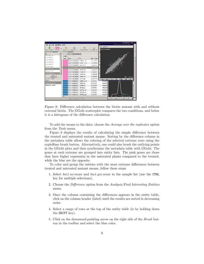
Figure 8: Difference calculation between the biotin mutant with and withoutexternal biotin. The GGobi scatterplot compares the two conditions, and belowit is a histogram of the difference calculation.

To add the means to the data: choose the Average over the replicates optionfrom the Tools menu.

Figure 8 displays the results of calculating the simple difference betweenthe treated and untreated mutant means. Sorting by the difference column inthe metadata table allows the coloring of the selected extreme rows using theexploRase brush button. Alternatively, one could also brush the outlying pointsin the GGobi plots and then synchronize the metadata table with GGobi. Thegenes at each extreme are grouped into entity lists. The pink genes are thosethat have higher expression in the untreated plants compared to the treated,while the blue are the opposite.

To color and group the entities with the most extreme differences betweentreated and untreated mutant means, follow these steps:

1. Select bio1.no.mean and bio1.yes.mean in the sample list (use the CTRL

key for multiple selections).

2. Choose the Difference option from the Analysis/Find Interesting Entitiesmenu.

3. Once the column containing the differences appears in the entity table,click on the column header (label) until the results are sorted in decreasingorder.

4. Select a range of rows at the top of the entity table (ie by holding downthe SHIFT key).

5. Click on the downward-pointing arrow on the right side of the Brush but-ton in the toolbar and select the blue color.

9

6. Click the Brush button to color the selected rows blue.

7. Click the Create List button and enter “biotin-activated” into the entrythat appears in the entity list panel.

8. Click on the header of the difference column again to resort the rows ofthe entity table so that the rows are in increasing order.

9. Repeat steps 4-7 but use pink rather than blue as the brush color andenter “biotin-repressed” when creating the list.

10. To sort the rows in the entity table by their list membership, click on theheader of the “List” column.

The scatterplot at the top-right of Figure 8 compares the two means, showingthat the colored observations are indeed outliers. Below the scatterplot is ahistogram showing the distribution of the difference.

To create the GGobi plots:

1. Focusing on the GGobi control panel window, select the New ScatterplotDisplay option from the Displays menu.

2. Select the two mean variables by clicking on the X button next to thebio1.no.mean label and the Y button next to the bio1.yes.mean label.

3. Select the New Scatterplot Display option (again) from the Displays menu.

4. To change the scatterplot to an ASH plot (histogram), select the 1D Plotfrom the View menu.

5. Click the X button next to the diff.bio1... variable, so that the histogramshows the distribution of the differences.

One possible way to verify that those genes are indeed dependent on biotintreatment would be to fit linear models using limma, including effects for thegenotype, biotin treatment, and their interaction.

To do this using the limma frontend in exploRase:

1. Choose the Linear modeling (limma) option from the Modeling menu.This should open the dialog shown on the left in Figure 6.

2. In the list of factors, select the checkbox for the interaction of genotypeand biotin. Note that this automatically selects the individual factors.

3. Click Apply to run limma.

Figure 9 shows the F values for the interaction of biotin and genotype. Thetable is sorted by the F value and filtered so that only the genes with the largestvalues (> 95) are included in the table. As one might expect, several of the pinkand blue genes have extreme F values, indicating that biotin treatment has agenotype-dependent effect on those genes.

To focus on the largest F values, as above:

10

Figure 9: Limma results for the biotin data. Only the entities with an F statistic> 95 for the interaction of genotype and biotin are displayed.

1. Click on the Filter label above the entity table, so that the filter GUI isshown.

2. Select F.genotype*biotin from the left-most combo box in the filter panel.

3. Change the second combo box to >.

4. Enter “95” into the text field to the right.

5. Click Apply to apply the filter rule (F.genotype*biotin > 95). Genes withan F value less than 95 are now excluded from the entity table.

6. Click the header of the “F.genotype*biotin” column to sort by it.

One outlier is easy to recognize even from the table: 13212 s at. The anno-tations in the table describe 13212 s at as a glycosyl hydrolase. The functionsof the other outlying genes, if known, may be found in the table, and if moreinformation is needed, clicking the AtGeneSearch button in the toolbar spawnsa web browser and queries the MetNetDB for additional details. This analysiscould continue along many paths. For example, one might search for genes thatare similar to the 13212 s at using the distance measures in exploRase (fromthe Analysis menu), or one might continue to inspect the output of limma usingGGobi graphics. This example demonstrates only a fraction of the potential ofexploRase.

11

5 Related work

exploRase is unique among open-source tools in its integration of interactivegraphics with R statistical analysis beneath a GUI designed especially for thesystems biologist. The commercial microarray analysis program GeneSpringlinks to R and Bioconductor and offers some interactive graphics. The freeprogram Cytoscape (Shannon et al., 2003) is designed for viewing and analyzingexperimental data in the context of biological networks and is integrated withR via plugins. However, it lacks interactive graphics outside of its networkdiagrams.

There are many examples of controlling R with a GUI, including severalin Bioconductor. The limmaGUI package (Smyth, 2005) provides a GUI thatleads the user from preprocessing microarray data to modeling it with limmaand producing reports. Unfortunately, limmaGUI lacks the interactive graphicsand breadth of analysis features of exploRase. The Bioconductor iSPlot packageprovides general interactive graphics using the R graphics engine but offers onlya small subset of GGobi’s functionality. Rattle (Williams, 2006) is an RGtk2-based GUI that leverages R as it guides the user through a wide range of datamining tasks.

6 Technical Design Considerations

exploRase is written purely in R, permitting easy integration with R analysispackages. This also enables other R packages to integrate with exploRase viaits public API.

The primary design consideration for the GUI is simplicity. There is noattempt to completely map the features of Bioconductor packages and GGobito the exploRase front-end. Rather, the GUI supports only a subset of thefeatures provided by the underlying packages, while augmenting the subset withshortcuts and conveniences. In order to provide its GUI, exploRase relies on theRGtk2 package (Lawrence, 2007a), a bridge from R to the GTK+ 2.0 cross-platform widget library (GTK+, 2007). RGtk2 allows exploRase to present,completely from within R, a visually pleasing, feature-rich GUI that is identicalacross all major computing platforms.

The rggobi package (Wickham and Lawrence, 2006) links R with GGobi.With rggobi, R packages are able to load data from R into GGobi, retrieveGGobi datasets into R, get and set the color of observations, create and configuredisplays, and more. exploRase uses rggobi to load high-throughput datasetsand synchronize the color of observations in GGobi plots with the colors in thebiological metadata table in the exploRase GUI. This provides the key visuallink between the GUI of exploRase and the visualizations of GGobi.

12

7 Acknowledgements

We thank Eve Wurtele, Heather Babka, Suh-yeon Choi, and others in the Met-Net group at Iowa State University for their helpful feedback in the developmentof exploRase. We also acknowledge our funding sources, NSF Arabidopsis 2010DB10209809 and DB10520267.

References

GTK+. The Gimp Tool Kit, 2007. URL http://www.gtk.org/.

M. Lawrence. RGtk2, 2007a. URL http://www.ggobi.org/rgtk2.

M. Lawrence. Explorase website, 2007b. URL http://www.metnetdb.org/

MetNet_exploRase.htm.

P. Shannon, A. Markiel, O. Ozier, N. S. Baliga, J. T. Wang, D. Ram-age, N. Amin, B. Schwikowski, and T. Ideker. Cytoscape: A SoftwareEnvironment for Integrated Models of Biomolecular Interaction Networks.Genome Res., 13(11):2498–2504, 2003. doi: 10.1101/gr.1239303. URLhttp://www.genome.org/cgi/content/abstract/13/11/2498.

G. K. Smyth. Limma: linear models for microarray data. In R. Gentleman,V. Carey, S. Dudoit, R. Irizarry, and W. Huber, editors, Bioinformatics andComputational Biology Solutions using R and Bioconductor, pages 397–420.Springer, 2005.

H. Wickham and M. Lawrence. rggobi, 2006. URL http://www.ggobi.org/

rggobi.

G. Williams. Rattle: gnome R data mining, 2006. URL http://rattle.

togaware.com/.

E. Wurtele, J. Li, L. Diao, H. Zhang, C. Foster, B. Fatland, J. Dickerson,A. Brown, Z. Cox, D. Cook, E. Lee, and H. Hofmann. Metnet: Software tobuild and model the biogenetic lattice of arabidopsis. Comp. Funct. Genom.,4:239–245, 2003.

13