Exploiting symmetries within constraint satisfaction searchcse.unl.edu/~choueiry/Documents/Meseguer-Torras-2001.pdf · These strategies are then applied to two highly symmetric

Artificial Intelligence 129 (2001) 133–163

Exploiting symmetrieswithin constraint satisfaction search ✩

Pedro Meseguer a,∗, Carme Torras b

a Institut d’Investigació en Intel.ligència Artificial, CSIC, Campus UAB, 08193 Bellaterra, Spainb Institut de Robòtica i Informàtica Industrial, CSIC-UPC, Gran Capità 2-4, 08034 Barcelona, Spain

Received 15 February 2000; received in revised form 28 February 2001

Abstract

Symmetry often appears in real-world constraint satisfaction problems, but strategies for exploitingit are only beginning to be developed. Here, a framework for exploiting symmetry within depth-firstsearch is proposed, leading to two heuristics for variable selection and a domain pruning procedure.These strategies are then applied to two highly symmetric combinatorial problems, namely theRamsey problem and the generation of balanced incomplete block designs. Experimental resultsshow that these general-purpose strategies can compete with, and in some cases outperform, previousmore ad hoc procedures. 2001 Elsevier Science B.V. All rights reserved.

Keywords:Symmetry; Constraint satisfaction; Heuristics; Nogoods

1. Introduction

Symmetry is present in many natural and artificial settings. A symmetry is a transforma-tion of an entity such that the transformed entity is equivalent to and indistinguishable fromthe original one. We can see symmetries in nature (a specular reflection of a daisy flower),in human artifacts (a central rotation of 180 degrees of a chessboard), and in mathematicaltheories (inertial changes in classical mechanics). The existence of symmetries in thesesystems allows us to generalize the properties detected in one state to all its symmetricstates.

Regarding constraint satisfaction problems (CSPs), many real problems exhibit somekind of symmetry, embedded in the structure of variables, domains and constraints. This

✩ This paper is an extended and updated version of [16], presented at the IJCAI-99 conference.* Corresponding author.E-mail addresses:[email protected] (P. Meseguer), [email protected] (C. Torras).

0004-3702/01/$ – see front matter 2001 Elsevier Science B.V. All rights reserved.PII: S0004-3702(01)0 01 04 -7

134 P. Meseguer, C. Torras / Artificial Intelligence 129 (2001) 133–163

means that their state space is somehow fictitiously enlarged by the presence of manysymmetric states. From a search viewpoint, it is advisable to visit only one among thosestates related by a symmetry, since either all of them lead to a solution or none does. Thismay cause a drastic decrease in the size of the search space, which would have a verypositive impact on the efficiency of the constraint solver.

Previous work on symmetric CSPs has been aimed at eradicating symmetries fromeither the initial problem state space or the explicit search tree as it is developed. Theformer approach, advocated by Puget [19], consists in reducing the initial state space byadding symmetry-breaking constraints to the problem formulation. The goal is to turnthe symmetric problem into a new problem without symmetries, but keeping the non-symmetric solutions of the original one. Although this ideal goal is seldom reached,the reductions attained are substantial enough to turn some hard combinatorial problemsinto manageable ones. For generic problem statements, the detection of symmetriesand the formulation of the ad hoc symmetry-breaking constraints is performed by hand[19]. Alternatively, in the context of propositional logic, existing symmetries and thecorresponding symmetry-breaking predicates can be computed automatically [6], althoughwith a high computational complexity.

The second approach, namely pruning symmetric states from the search tree asit develops, entails modifying the constraint solver to take advantage of symmetries.A modified backtracking algorithm appears in [3], where each expanded node is testedto assess whether it is an appropriate representative of all the states symmetric to it.Concerning specific symmetries, neighborhood interchangeable values of a variable arediscussed in [9], while value pruning after failure for strongly permutable variables isproposed in [20]. This last strategy can be seen as a particular case of the symmetryexclusion method introduced in [1] for concurrent constraint programming, and appliedto the CSP context in [11].

In this paper, we propose a third approach to exploit symmetries inside CSPs. The ideais to use symmetries to guide the search. More specifically, the search is directed towardssubspaces with a high density of non-symmetric states, by breaking as many symmetriesas possible with each new variable assignment. This is the rationale for our symmetry-breakingheuristic for variable selection, which can be theoretically combined with thepopular minimum-domain heuristic. The result of this combination is the new variety-maximizationheuristic for variable selection, which has been shown more effective thansymmetry-breaking or minimum-domain separatedly, and it has speeded up significantlythe solving process of CSPs with many symmetries. For problems without a solution,variable selection heuristics can do nothing to avoid revisiting symmetric states alongthe search. To cope with this shortcoming, we have developed several value pruningstrategies (in the spirit of the second approach mentioned above), which allow one toreduce the domain of the current or future variables. These strategies remove symmetricvalues, without removing non-symmetric solutions. In particular, there is a strategy basedon nogoods learned in previous search states. Problem symmetries allow us to keep limitedthe potentially exponential size of the nogood storage. This strategy has been shown veryeffective for hard solvable and unsolvable instances. Results for the Ramsey problem andfor the generation of balanced incomplete block designs (BIBDs) are provided. Once a setof symmetries is specified, our approach provides a general-purpose mechanism to exploit

P. Meseguer, C. Torras / Artificial Intelligence 129 (2001) 133–163 135

them within the search. Moreover, it can be combined with the two previous approachesand incorporated into any depth-first search procedure.

The paper is structured as follows. In Section 2, we introduce some basic concepts.Section 3 presents the symmetry-breaking heuristic and its combination with the minimum-domain one, generating the variety-maximization heuristic. Section 4 details severalstrategies for symmetric value pruning along the search, especially those based on nogoodrecording. Section 5 is devoted to the Ramsey and BIBD problems. Finally, Section 6 putsforth some conclusions and prospects for future work.

2. Basic definitions

2.1. Constraint satisfaction

A finite CSP is defined by a triple (X ,D,C), where X = {x1, . . . , xn} is a set of n

variables, D = {D(x1), . . . ,D(xn)} is a collection of domains, D(xi) is the finite set ofpossible values for variable xi , and C is a set of constraints among variables. A constraint ci

on the ordered set of variables var(ci) = (xi1, . . . , xir(i)) specifies the relation rel(ci) of the

allowedcombinations of values for the variables in var(ci). An element of rel(ci) is a tuple(vi1 , . . . , vir(i)

), vi ∈ D(xi). An element of D(xi1 ) × · · · × D(xir(i)) is called a valid tuple

on var(ci). A solutionof the CSP is an assignment of values to variables which satisfiesevery constraint. A nogoodis an assignment of values to a subset of variables which doesnot belong to any solution. Typically, CSPs are solved by depth-first search algorithms withbacktracking. At a point in search, P is the set of assigned or pastvariables, and F is theset of unassigned or futurevariables. The variable to be assigned next is called the currentvariable.

A classical example of CSP is the n-queens problem. It consists in placing n chessqueens on an n × n chessboard in such a way that no pair of queens is attacking oneanother. Constraints come from chess rules: no pair of queens can occur at the same row,column or diagonal. This problem is taken as running example throughout the paper.

2.2. Symmetries

A symmetryon a CSP is a collection of n + 1 bijective mappings {θ, θ1, . . . , θn} definedas follows,

• θ is a variable mapping, θ :X →X ,• {θ1, . . . , θn} are domain mappings, θi : D(xi) → D(θ(xi)),• constraints are transformed by the adequate combination of variable and domain

mappings; a constraint ci is transformed into cθi , with var(cθ

i ) = (θ(xi1), . . . , θ(xir(i)))

and rel(cθi ) = {(θi1(vi1 ), . . . , θir(i)

(vir(i)))},

such that the set C remains invariant by the action of the symmetry, i.e., ∀cj ∈ C , thetransformed constraint cθ

j is in C . There exists always a trivial symmetry, that in which thevariable mapping and the domain mappings are all the identity. The remaining symmetries,those interesting for our purposes, will be referred to as nontrivial symmetries. Moreover,


Fig. 1. Central rotation of 180 degrees is a symmetry of the 5-queens problem.

when no ambiguity may occur, we will denote a symmetry {θ, θ1, . . . , θn} by its variablemapping θ .

Note that the above definition of symmetry applies to CSPs, i.e., to problems formulatedin terms of a triple (X ,D,C), and not to problems in general. To make this point clear,consider the n-queens problem, which admits at least nine different problem formulationsas a CSP [17]. These formulations vary in the number of variables, sizes of the domains,and constraint set. They specify different CSPs and, as such, it is not surprising that theyhave different symmetries.

Let us consider the most widely used formulation, namely that in which variables arechessboard rows and domains are column indices. Fig. 1 shows an example of a symmetryusing this formulation in the case of 5 queens. It is a central rotation of 180 degrees, whichexchanges variables x1 with x5 and x2 with x4, and maps domains with the functionθi(v) = 6 − v, i = 1, . . . , 5. This transformation is a symmetry because the mappingson variables and domains are bijective, and the set of constraints is left invariant by thetransformation of variables and values. For example, the transformed constraint cθ

12 iscomputed as follows,

var(cθ

12

) = (θ(x1), θ(x2)

) = (x5, x4) = var(c45),

rel(cθ

12

) = {(θ1(1), θ2(3)), (θ1(1), θ2(4)), (θ1(1), θ2(5)), (θ1(2), θ2(4)),

(θ1(2), θ2(5)), (θ1(3), θ2(1)), (θ1(3), θ2(5)), (θ1(4), θ2(1)),

(θ1(4), θ2(2)), (θ1(5), θ2(1)), (θ1(5), θ2(2)), (θ1(5), θ2(3))}

= {(5, 3), (5, 2), (5, 1), (4, 2), (4, 1), (3, 5), (3, 1), (2, 5), (2, 4), (1, 5),

(1, 4), (1, 3)}

= rel(c45).

Thus, cθ12 = c45. Two other nontrivial symmetries of this CSP formulation of 5-queens are

the reflections about the horizontal and vertical axes, as depicted in Fig. 2. The remainingfour symmetries of the chessboard are not symmetries of this formulation.

Now, let us turn to the formulation of n-queens where each queen is a variable whosedomain contains all the squares of the chessboard. The eight symmetries of the chessboardand all permutations of queens are symmetries of this particular CSP formulation.

Taken together, the two examples above illustrate the remark we made that our definitionof symmetry applies to CSP formulations and not to problems in general. Such symmetriescan be viewed as mapping a triple (X ,D,C) onto itself, which is needed to stay within


Fig. 2. Two other symmetries of the 5-queens problem. Top-right: reflection about the vertical axis. Bottom-left:reflection about the horizontal axis.

the formulation. Thus, transformations that change variables into values and vice versa, aswould be required to represent a rotation of 90 degrees under the formulation in Fig. 1, arenot allowed within our framework.

Following [22], we say that two variables xi , xj are symmetricif there exists asymmetry θ such that θ(xi) = xj . This concept generalizes the previous definition of strongpermutability [20]: xi and xj are strongly permutable if they play exactly the same role inthe problem, i.e., if there exists a symmetry φ such that its only action is exchanging xi

with xj (φ(xi) = xj , φ(xj ) = xi , φ(xk) = xk , ∀k = i, j , φk = I , ∀k, I being the identityfunction). We say that two values a, b ∈ D(xi) are symmetricif there exists a symmetry θ

such that θ(xi) = xi and θi(a) = b. This concept generalizes previous definition of valueinterchangeability [9]: a and b are neighbourhood interchangeable if they are consistentwith the same set of values, i.e., if there exists a symmetry φ such that its only action isexchanging a with b (φ = I , φi(a) = b, φi(b) = a, φi(c) = c, ∀c = a, b, φk = I , ∀k = i).

The set of symmetries of a problem forms a group with the composition operator[22]. Because of this, it can be shown that the symmetry relation between variables isan equivalence relation. The existence of this equivalence relation divides the set X inequivalence classes, each class grouping symmetric variables. Domains are also dividedinto equivalence classes by symmetries acting on values only (with identity variablemapping). Regarding the 5-queens problem under the formulation of Fig. 1, there are threeequivalence classes of variables: {x1, x5}, {x2, x4} and {x3}. Concerning values, there arealso three equivalence classes: {1, 5}, {2, 4} and {3}. Neither strongly permutable variablesnor neighbourhood interchangeable values exist in this problem.

2.3. Symmetries in search

Symmetries can occur in the initial problem formulation, and also in any search states, characterized by an assignment of past variables plus the current domains of futurevariables. State s defines a subproblem of the original problem, where the domain of each


past variable is reduced to its assigned value and the relation rel(ci) of each constraint ci

is reduced to its valid tuples with respect to current domains. A symmetry holdsat state s

if it is a symmetry of the subproblem occurring at s. A symmetry holding at s is said to belocal to s if it does not change the assignments of past variables. 1 The set of symmetrieslocal to s forms a group with the composition operation. A symmetry holding at the initialstate s0 is called a global symmetry of the problem. Any global symmetry is local to s0,the state where the set of past variables is empty. Symmetries depicted in Figs. 1 and 2 areglobal symmetries of the 5-queens problem. An important property of symmetries is thatthey are solution-preserving, transforming solutions into solutions.

Let s be a search state with symmetry θ local to it, and s′ a successor state. We saythat the assignment occurring between s and s′ breakssymmetry θ if θ is not local tos′. Typically, symmetries local to s are global symmetries that have not been brokenby the assignments occurring between s0 and s. However, this is not always the case.New symmetries may appear in particular states. For the 5-queens problem, some stateswith local symmetries appear in Fig. 3. State sa keeps as local the three nontrivial globalsymmetries of the problem, since none is broken by the assignment of x3. State sb keepsas local the reflection about the vertical axis only, since the central rotation and the otherreflection are broken by the assignment of x1. In state sc , all nontrivial global symmetriesare broken by the assignment of x1 but a new symmetry appears: a central rotation of 180degrees on the 4 × 4 subboard involving variables from x2 to x5 and columns from 2 to 5.A broken symmetry can be restored by another assignment, as it can be seen in Fig. 4. In

Fig. 3. Three states of the 5-queens problem, with different types of local symmetries.

Fig. 4. The central rotation symmetry is broken in sa and restored in sb .

1 Notice that this definition differs from the one appearing in [16] in that the mapping on past variables is notrequired to be the identity.


state sa the assignment of x1 breaks the central rotation symmetry, which is restored afterthe assignment of x5 in state sb .

3. Heuristics based on symmetries

3.1. The symmetry-breaking heuristic

We argue that breaking as many symmetries as possible at each stage is a good strategy tospeed up the search. Let us first illustrate some points with a simple example. Consider theequation x + y2z2 = 2, where all variables take values in {−1, 0, 1}. There are 5 nontrivialsymmetries, derived from combining the permutability of y and z, with the sign irrelevanceof both y and z. They can be briefly indicated as follows:

(1) θ(y) = z, θ(z) = y;(2) θy = −I ;(3) θz = −I ;(4) θy = −I , θz = −I ;(5) θ(y) = z, θ(z) = y , θy = −I , θz = −I ;

where I is the identity mapping, and all the entries not specified are also the identity.Symmetry (1) is a permutation of variables, symmetries (2)–(4) interchange values,

whereas symmetry (5) entails changes in both variables and values. Note that variables y

and z are involved in (4) nontrivial symmetries each, while variable x is involved in none.Fig. 5 displays two search trees for that equation, following the variable orderings x, y, z

and y, z, x . In the upper tree, no symmetry is broken after assigning x , and thereforeall symmetries act inside each subtree at the first level, leading to a low density of

Fig. 5. Search tree generated to solve the equation x + y2z2 = 2 under two variable orderings. Symmetric statesoriginated by permutable variables are connected by shadowed lines, while those arising from interchangeablevalues are joined by broken lines. Solutions are marked with squares.


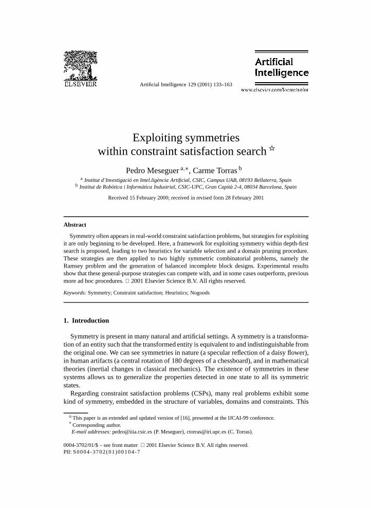
Fig. 6. Effect of pruning on the search trees in Fig. 5.

distinct final states considered whatever the value assigned to x . This can be more easilyvisualized in Fig. 6, where states symmetric to a previously expanded one have beenremoved. There are only 3 distinct states among the 9 final states considered in each ofthe three subtrees resulting from assigning a value to x . For the leftmost subtree, these are(x, y, z) = (−1,−1,−1), (−1,−1, 0) and (−1, 0, 0).

Under the second ordering, represented in the lower tree of Fig. 5, symmetries (1), (2),(4) and (5) are broken after assigning y , and thus only states replicated by symmetry (3)appear inside subtrees at the first level. Concretely, there are 6 distinct states among the9 final states considered in each of the three subtrees resulting from assigning a value toy . For the leftmost subtree, these are (y, z, x) = (−1,−1,−1), (−1,−1, 0), (−1,−1, 1),(−1, 0,−1), (−1, 0, 0) and (−1, 0, 1). The density of distinct final states in each subtree atthe first level is thus much higher here (2/3) than under the first ordering (1/3). Again notethat this is independent of the value assigned to y . If, in Fig. 6, the subtree correspondingto y = 0 or y = 1 would have been expanded first, instead of that for y = −1, then thecorresponding subtree would equally have six distinct final states.

When one has no a priori knowledge on the distribution of solutions across the statespace, trying to maximize the density of distinct final states considered at each searchstage looks like a good strategy. This is the rationale for the following variable selectionheuristic.

Symmetry-breaking heuristic. Select for assignment the variable involved in the greatestnumber of symmetries local to the current state.

The above greedy heuristic, which tries to break as many symmetries as possible at eachnew variable assignment, produces the following benefits:


(1) Wider distribution of solutions. Symmetric solutions will spread out under differentsubtrees instead of grouping together under the same subtree. This increases thelikelihood of finding a solution earlier. Take the equation in the example above.It has four solutions, namely (x = 1, y = −1, z = −1), (x = 1, y = −1, z = 1),(x = 1, y = 1, z = −1) and (x = 1, y = 1, z = 1). Under the first variable ordering,they are all grouped below the rightmost subtree, while under the second, theyspread two subtrees.

(2) Lookahead of better quality. A lookahead algorithm prunes future domains takinginto account past assignments. When symmetries on future variables are present,some of the lookahead effort is unproductive. If there is a symmetry θ such thatθ(xj ) = xk , with xj , xk ∈ F , after lookahead on D(xj ), lookahead on D(xk)

is obviously redundant because it will produce results equivalent (through θ ) tolookahead on D(xj ). If no symmetries are present, no lookahead effort will beunproductive. Therefore, the more symmetries are broken, the less unproductiveeffort lookahead performs. When the number of symmetries is high, savings inunproductive lookahead effort can be substantial.

(3) More effective pruning. Several techniques to prune symmetric states have beenproposed in the literature, such as those based on neigbourhood interchangeablevalues [9] and on permutable variables [20]. The proposed heuristic amplifies theeffect of any pruning technique by moving its operation upwards in the search tree.Fig. 6 shows the result of applying the two types of pruning mentioned to the searchtrees displayed in Fig. 5. The 10 nodes expanded under the variable ordering x, y, z,are reduced to only 6 nodes when the heuristic is in use. Moving pruning upwardstends to produce smaller branching factors in the higher levels of the search tree,resulting in thinner trees.

It is worth noting that points (2) and (3) above apply also to problems without asolution. Empirical results supporting these claims are provided in Section 3.3 for thelayout problem.

3.2. The variety-maximization heuristic

Let us return to the example in Figs. 5 and 6. The variable ordering y, z, x suggestedby the symmetry-breaking heuristic is the one leading to subtrees with highest density ofdistinct final states, and, after pruning, it produces the thinnest tree. This is the effect of theheuristic on a problem where all domains have equal sizes. Now consider the same problembut reducing the domain of x to only one value {−1}. Then, under the variable orderingx, y, z, only the leftmost branch of the upper tree in Fig. 5 would be developed, while underthe ordering y, z, x , the whole lower tree in Fig. 5 would be developed, although only forthe leaves labelled −1. The effect of pruning could likewise be visualized by looking atFig. 6. It is clear that, in this case, the best option is the ordering x, y, z since it leads to athinner tree to start with (13 nodes against 21 for the other ordering) and also after pruning(6 nodes against 14). Thus, in this case, the well-known minimum-domain heuristic woulddo better than the symmetry-breaking one. And the question arises: When should one or theother heuristic be applied? Even more useful, is there a way of combining both heuristicsthat outperforms the isolated application of each of them?


To try to answer these questions, let us first recall the interpretations provided for thegood performance of the minimum-domain heuristic. The most widespread one is thatthe heuristic implements the fail-first principle, and thus minimizes the expected depth ofeach search branch [14]. Smith and Grant [23] tested this interpretation experimentallyby comparing the behaviour of several heuristics with increasing fail-first capabilities andconcluded that the success of minimum-domain may not necessarily be due to the factthat it implements fail first. Often the effect of shallow branches is counteracted by highbranching factors. Thus, another interpretation puts the emphasis on the minimization ofthe branching factor at the current node [21]: since the minimum-domain heuristic forcesthe search tree to be as narrow as possible in its upper levels, the expected number ofnodes generated is minimized. This holds for problems both with and without a solution.Further along this line, we may view the minimum-domain heuristic as following a least-commitment principle, i.e., it chooses the variable that partitions the state space in lessnumber of subspaces, so that each subspace is larger (contains more states) than if anothervariable would have been selected. The resulting search trees are, again, as narrow aspossible in their upper levels, so the aforementioned node minimization still holds. Butnow, for problems with a solution, another factor may play a favourable role: in a largersubspace it is more likely to find a solution. A related interpretation was put forth in[10] under the rationale of minimizing the constrainedness of the future subproblem:underconstrained problems tend to have many solutions and be easy to solve.

In dealing with highly symmetric problems, however, the largest subspace doesnot necessarily contain more distinct final states than a smaller one. Thus, the least-commitment principle has here to be applied in terms of distinctfinal states. What is neededis a strategy that selects the variable leading to consider the highest number of distinct finalstates, but what we have is:

• the minimum-domain heuristic, which selects the variable that maximizes the numberof final states considered, and

• the symmetry-breaking heuristic, which chooses the variable that maximizes thedensityof distinctfinal states considered.

In the following, we develop a framework for the combination of both heuristics,based on the two basic types of symmetry, namely interchangeable values and stronglypermutable variables. As mentioned in Section 2.2, both types of symmetry induceequivalence classes in the domains and set of variables, respectively. Let x1, . . . , xk be therepresentatives of the equivalence classes of future variables at a given search stage, ci bethe size of the equivalence class to which xi belongs, and di be the number of equivalenceclasses in D(xi). In other words, ci is the number of original variables strongly permutablewith xi , including itself; and di is the number of non-interchangeable values that can beassigned to xi .

Let us calculate the number of distinct final states considered at this search stage,where “distinctiveness” is here taken to mean that no two states can be made equal byinterchanging values or permuting variables. For each equivalence class i , we need toassign ci variables, each of which can take di values. If variables were not permutable,the number of joint assignments would be d

ci

i . However, since the variables are stronglypermutable, two assignments related by a permutation are not distinct. Therefore, thenumber of distinct joint assignments is given by the combinations with repetition of di


elements taken ci at a time. Describing this as an occupancy problem, we need to place ci

balls into di buckets (i.e., assign ci variables, each to one of the possible di values). Theformula to obtain the number of possible placements (i.e., distinct assignments) is [8] 2:(di+ci−1

ci

).

The total number of distinct final states, considering all the equivalence classes ofvariables, is thus given by the product

k∏i=1

(di + ci − 1

ci

).

If the next assigned variable belongs to the equivalence class represented by xi0 , then

its corresponding term decreases from(di0+ci0 −1

ci0

)to

(di0+ci0 −2ci0−1

), since the equivalence

class i0 loses an element. Thus, the number of distinct final states considered after variableassignment will be:

(di0+ci0 −2ci0−1

)(di0+ci0 −1

ci0

)k∏

i=1

(di + ci − 1

ci

).

We like to find the i0 that maximizes this expression, i.e.,

maxi

(di+ci−2

ci−1

)(di+ci−1

ci

) ,

which can be developed as

maxi

(di+ci−2)!(di−1)! (ci−1)!

(di+ci−1)!(di−1)! ci !

,

leading to

maxi

ci

di + ci − 1,

which is the same as

mini

di − 1

ci

.

By taking the index i0 that realizes this minimum, and assigning a variable in theequivalence class of xi0 , we attain our purpose of considering a subspace with themaximum number of distinct final states, i.e., states containing neither interchangeable

2 Feller [8, p. 38] provides an ingenous and elegant proof: Let us represent the balls by stars and indicate thedi buckets by the di spaces between di + 1 bars. Thus, | ∗ ∗ ∗ | ∗ |||| ∗ ∗ ∗ ∗| is used as a symbol for a distributionof ci = 8 balls in di = 6 buckets with occupancy numbers 3, 1, 0, 0, 0, 4. Such a symbol necessarily starts andends with a bar, but the remaining di − 1 bars and ci stars can appear in an arbitrary order. In this way it becomesapparent that the number of distinguishable distributions equals the number of ways of selecting ci places out ofci + di − 1, i.e.,

(di+ci−1ci

).


values nor strongly permutable variables. This is what the following variable selectionheuristic does.

Variety-maximization heuristic. Select for assignment a variable belonging to theequivalence class for which the ratio di−1

ciis minimum.

When all the equivalence classes of variables are of the same size, then the synthesizedheuristic reduces to the minimum-domain one. On the other hand, when all domains havethe same number of non-interchangeable values, then the heuristic chooses a variablefrom the largest equivalence class; this is exactly what the symmetry-breaking heuristicwould do. To show this, let us quantify the symmetries broken by a given assignment.Since all permutations inside each class of strongly permutable variables lead to localsymmetries, the total number of such symmetries is c1! c2! · · ·ck! If we assign a variablefrom equivalence class i , then the number of remaining symmetries after the assignmentwill be: c1! c2! · · · (ci − 1)! · · ·ck! Thus, the ratio of remaining symmetries over the totalwill be 1/ci . To maximize symmetry-breaking, we have to determine

min1�i�k

1

ci

which is the same as saying that we have to select a variable from the largest equivalenceclass.

In sum, by applying the least-commitment principle in terms of maximizing the numberof distinct final states considered at each search stage, we have come up with a clean wayof combining the minimum-domain and the symmetry-breaking heuristics, so as to extractthe best of both along the search.

3.3. An example: The layout problem

To illustrate variety-maximization and its relation with minimum-domain, let us considerthe layout problem [12] defined as follows: given a grid, we want to place a number ofpieces such that every piece is completely included in the grid and no overlapping occursbetween pieces. An example of this problem appears in Fig. 7, where three pieces haveto be placed inside the proposed grid. As CSP, each piece is represented by one variablewhose domain is the set of allowed positions in the grid. There is a symmetry betweenvariables y and z, which are strongly permutable. No symmetry between values exists.

Fig. 7 contains two search trees developed by the forward checking algorithm followingtwo variable ordering heuristics. The left tree corresponds to the minimum-domainheuristic, which selects x as first variable (|Dx | = 3 while |Dy | = |Dz| = 4), and y

and z as second and third variables in all the branches. The right tree corresponds tothe variety-maximization heuristic. Instead of x , variety-maximization selects y as firstvariable because 4−1

2 < 3−11 , in agreement with symmetry-breaking. The assignment of y

breaks the problem symmetry, so from this point variety-maximization follows minimum-domain. This can be seen in the rightmost branch after assigning y . Variable z is selectedas next variable because after forward checking lookahead |Dz| = 2 while |Dx | = 3.This example shows how variety-maximization combines both symmetry-breaking and


Fig. 7. The layout problem and two search trees developed by forward checking with minimum-domain (left) andvariety-maximization (right) heuristics.

minimum-domain heuristics, following at each point the most advisable option (dependingon the existing symmetries and domain cardinalities).

To test the benefits that symmetry-breaking (embedded in variety-maximization) bringsover minimum-domain, as listed at the end of Section 3.1, we have solved a larger instanceof this problem. In a 6 × 6 square grid, we want to place 4 pieces of size 2 × 2, plus 4pieces of size 5 × 1. As CSP, each piece corresponds to one variable, with domains ofcardinalities 25 for 2 × 2 pieces and 24 for 5 × 1 pieces. Variables corresponding to equalpieces are strongly permutable. Therefore, there are two equivalence classes of 4 variableseach. The minimum-domain heuristic selects two 5 × 1 pieces as the first two variablesof the search tree. At the second level, there are 242 = 576 nodes, 24 of which lead toa solution. The variety-maximization heuristic selects a 5 × 1 piece as the first variableand a 2 × 2 piece as second variable. At the second level there are 24 × 25 = 600 nodes,32 of which lead to a solution. The density of nodes leading to a solution at the secondlevel following minimum-domain is 24

576 = 0.0417, and following variety-maximization is32600 = 0.059. Thus, variety-maximization yields a better distribution of solutions in thesearch tree than minimum-domain, increasing the likelihood of finding a solution earlier.

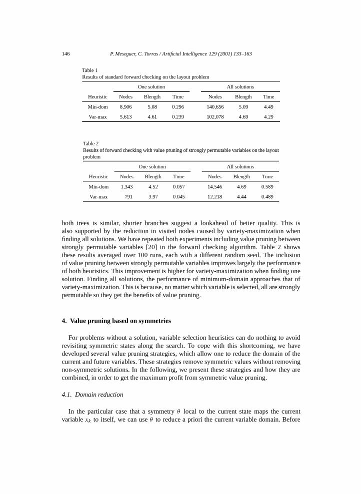
We have solved this problem instance using the standard forward checking algorithm,finding the first solution and all solutions, in successive experiments. Values are selectedrandomly. Table 1 shows the results averaged over 100 runs, each with a different randomseed. We observe that, both in finding one and all solutions, variety-maximization visits lessnodes and requires less CPU time than minimum-domain. In addition, Blength records theaverage length of branches not leading to a solution. We see that variety-maximizationgenerates shorter branches than minimum-domain. Given that the branching factor of


Table 1Results of standard forward checking on the layout problem

One solution All solutions

Heuristic Nodes Blength Time Nodes Blength Time

Min-dom 8,906 5.08 0.296 140,656 5.09 4.49

Var-max 5,613 4.61 0.239 102,078 4.69 4.29

Table 2Results of forward checking with value pruning of strongly permutable variables on the layoutproblem

One solution All solutions

Heuristic Nodes Blength Time Nodes Blength Time

Min-dom 1,343 4.52 0.057 14,546 4.69 0.589

Var-max 791 3.97 0.045 12,218 4.44 0.489

both trees is similar, shorter branches suggest a lookahead of better quality. This isalso supported by the reduction in visited nodes caused by variety-maximization whenfinding all solutions. We have repeated both experiments including value pruning betweenstrongly permutable variables [20] in the forward checking algorithm. Table 2 showsthese results averaged over 100 runs, each with a different random seed. The inclusionof value pruning between strongly permutable variables improves largely the performanceof both heuristics. This improvement is higher for variety-maximization when finding onesolution. Finding all solutions, the performance of minimum-domain approaches that ofvariety-maximization. This is because, no matter which variable is selected, all are stronglypermutable so they get the benefits of value pruning.

4. Value pruning based on symmetries

For problems without a solution, variable selection heuristics can do nothing to avoidrevisiting symmetric states along the search. To cope with this shortcoming, we havedeveloped several value pruning strategies, which allow one to reduce the domain of thecurrent and future variables. These strategies remove symmetric values without removingnon-symmetric solutions. In the following, we present these strategies and how they arecombined, in order to get the maximum profit from symmetric value pruning.

4.1. Domain reduction

In the particular case that a symmetry θ local to the current state maps the currentvariable xk to itself, we can use θ to reduce a priori the current variable domain. Before


instantiating xk , equivalence classes of symmetric values in D(xk) by θ can be computed,producing Q1,Q2, . . . ,Qek equivalence classes. A new domain, D′(xk) is defined as

D′(xk) = {w1,w2, . . . ,wek }such that each wi is a representative for the class Qi . Now, the current variable xk takesvalues from D′(xk) in the following form. If xk takes value wi and generates solution S,there is no reason to test other values of Qi , because they will generate symmetric solutionsto S by θ . On the other hand, if value wi fails, there is no point in testing other values ofQi because they will fail as well. In this case, all values of Qi are marked as tested. Oncethe current variable has been selected, this strategy allows to reduce its domain to non-symmetric values, provided the adequate symmetry θ exists. When backtracking jumpsover xk , equivalence classes are forgotten and the previous D(xk) is taken as the domainfor xk .

An example of this domain reduction arises in the pigeon-hole problem: locating n

pigeons in n − 1 holes such that each pigeon is in a different hole. This problem isformulated as a CSP by associating a variable xi to each pigeon, all sharing the domain{1, . . . , n − 1}, under the constraints xi = xj , 1 � i, j � n, i = j . Among others, thisproblem has a collection of symmetries in the domains

∀i, ∀a, a′ ∈ D(xi) a = a′, ∃θ, θ = I, θi(a) = a′, θi(a′) = a,

where I is the identity mapping. If variables and values are considered lexicographically,before assigning x1 all values in D(x1) form a single equivalence class. Then, D′(x1) ={1}. Performing search by forward checking, value 1 is removed from all future domains.Considering x2, all its values form a single equivalence class, D′(x2) = {2}. Again,lookahead removes value 2 from all future domains. Considering x3, all its remainingvalues form a single equivalence class, D′(x3) = {3}, etc. This process goes on untilassigning (xn−1, n−1), when lookahead finds an empty domain in D(xn), so backtrackingstarts. At that point, all domains of past and current variables have been reduced to a singlevalue, which is currently assigned. Backtracking does not find any other alternative valueto test in any previous variable, so it ends with failure when x1 is reached. Only the leftmostbranch of the search tree is generated, and the rest of the tree is pruned.

4.2. Value pruning through nogood recording

A nogoodis an assignment of values to a subset of variables which does not belong toany solution. Before search, a set of nogoods is determined by the constraints as the setof forbidden value tuples. During search, new nogoods are discovered by the resolution ofnogoods responsible of dead-ends. For example, in Fig. 8, the forward checking algorithmfinds a dead-end in the 5-queens problem (D(x4) = ∅). By the resolution of the nogoodsassociated with every pruned value of D(x4), we get the new nogood,

(x1, 1)(x2, 5)(x3, 2)

which means that variables x1, x2 and x3 cannot simultaneously take the values 1, 5 and 2,respectively. Often nogoods are written in oriented form as,

(x1 = 1) ∧ (x2 = 5) ⇒ (x3 = 2)


Fig. 8. Nogood resolution in a dead-end for the 5-queens problem.

where the variable at the right-hand side is the last variable among the variables ofthe nogood that has been instantiated. This variable will be the one changed first whenperforming backtracking, which is needed to guarantee completeness of tree-searchalgorithms (see [2] for a detailed explanation of nogood resolution).

4.2.1. Value pruning due to symmetric nogoodsLet p = (x1, v1)(x2, v2) . . . (xk, vk) be a nogood found during search and θ a global

symmetry of the considered problem. It is easy to see that the tuple θ(p), defined as(θ(x1), θ1(v1))(θ(x2), θ2(v2)) · · · (θ(xk), θk(vk)), is also a nogood. Let us suppose thatθ(p) is not a nogood, that is, it belongs to a solution S. Given that θ−1 is also a problemsymmetry and problem solutions are invariant through symmetries, θ−1(S) is also asolution. But θ−1(S) contains p, in contradiction with the first assumption that p is anogood. Therefore, θ(p) is a nogood. Intuitively, θ(p) is the nogood that we would obtainfollowing a search trajectory symmetric by θ to the current trajectory. An example of thisappears in Fig. 9.

Given that we can generate nogoods using previously found nogoods and globalsymmetries of the problem, we propose to learn nogoods during search in the followingform:

(1) We store the new nogoods found during search.(2) At each node, we test if the current assignment satisfies some symmetric nogood,

obtained by applying a global symmetry to a stored nogood. If it does, the value ofthe current variable is unfeasible so it can be pruned. Values removed in this wayare restored when backtracking jumps above their corresponding variables.

Nogood recording in search presents two main issues: storage size and overhead [7].Regarding the storage space required, it may be of exponential size which could render thestrategy inapplicable in practice. The usual way to overcome this drawback is to store notall but a subset of the nogoods found, following different strategies: storing nogoods ofsize lower than some limit, fixing in advance the storage capacity and using some policyfor nogood replacement, etc. However, this important drawback has been shown to besurmountable in practice due to the following fact: a new nogood is never symmetric to analready stored nogood. Otherwise, the assignment leading to this new nogood would havebeen found unfeasible, because of the existence of a symmetric nogood, and it would havebeen pruned before producing the new nogood. If the number of global symmetries is highenough, this may cause a very significant decrement in the number of stored nogoods.

Regarding the overhead caused by nogood recording, it has two main parts: nogoodrecording and testing against symmetric nogoods. Nogood recording is a simple process


Fig. 9. Symmetric nogoods in the 5-queens problem. Left-right symmetry: reflection about the vertical axis.Up-down symmetry: reflection about the horizontal axis.

performed on a subset of the visited nodes, causing little overhead. However, testing eachnode against symmetric nogoods could mean checking an exponential number of nogoodsper node, which would severely degrade performance, eliminating any possible savingscaused by value removal. To prevent this situation, we restrict the number of symmetricnogoods against which the current node is tested, following two criteria:

(1) A subset of all global symmetries are used for symmetric nogood generation. Thecomposition of this subset is problem dependent (see Section 5 for further details).

(2) A subset of stored nogoods is considered for symmetric nogood generation. If xi isthe current variable and θ is a global symmetry, only nogoods containing θ(xi) inits right-hand side are considered.

Nevertheless, there are some particular cases where we can prune values withoutchecking stored nogoods, as explained in the following subsection.

4.2.2. Symmetric nogoods at the current branchLet s be a state defined by the assignment of past variables {(xi, vi)}i∈P , θ a symmetry

local to s, and xk the current variable. If after the assignment of xk the nogood p is found:

p =∧

j∈P ′, P ′⊆P

(xj , vj ) ⇒ (xk = vk)

it is easy to see that θ(p) is also a nogood. If p is a nogood, it means that it violatesa constraint c. By the definition of symmetry, θ(p) violates the symmetric constraint cθ .Therefore, θ(p) is also a nogood. The interesting point is that θ(p) also holds at the currentstate. Effectively,


Fig. 10. Symmetric nogoods by central rotation of 180 degrees in the subboard including variables x2 to x5 andcolumns 2 to 5.

θ(p) =∧

j∈P ′, P ′⊆P

(θ(xj ), θj (vj )

) ⇒ (θk(xk) = θk(vk)

)

=∧

j∈P ′′, P ′′⊆P

(xj , vj ) ⇒ (θk(xk) = θk(vk)

)

since all variables in the left-hand side of p are past variables, so they are mapped to otherpast variables and their assignments are not changed by θ . Therefore, at this point we canremove θk(vk) (the value symmetric to vk ) from D(θ(xk)), because it cannot belong toany solution including the current assignment of past variables. If all values of xk are triedwithout success and the algorithm backtracks, all values removed in this way should berestored. If xk is involved in several symmetries, this reasoning holds for each of themseparately. Thus, this strategy can be applied to any variable symmetric to xk .

This strategy of value removal after failure provides further support to the symmetry-breaking heuristic of Section 3.1. The more local symmetries a variable is involved in,the more opportunities it offers for symmetric value removal in other domains if a failureoccurs. This extra pruning is more effective if it is done at early levels of the search tree,since each pruned value represents removing a subtree on the level corresponding to thevariable symmetric to the current one.

An example of this pruning capacity appears in Fig. 10: further resolution of the nogoodsof x3 in Fig. 8 produces the nogood (x1 = 1) ⇒ (x2 = 5). The rotation of 180 degrees ofthe subboard including variables x2 to x5 and columns 2 to 5, is a symmetry local to thestate after the assignment (x1, 1). Therefore, applying this symmetry to the nogood, a newnogood is obtained:

(x1 = 1) ⇒ (x5 = 2)

which is a justification to prune value 2 from D(x5).

4.3. Combination of pruning strategies

The three pruning strategies mentioned, namely(i) domain reduction,

(ii) value pruning due to symmetric nogoods, and


(iii) value pruning due to symmetric nogoods at the current branch,can be combined to obtain the maximum profit in future domain reduction. The domain ofthe current variable is reduced (assuming that the adequate symmetry exists). If, for somereason (lookahead or symmetric nogood existence), its current value is discarded, all valuesof the same equivalence class are also discarded. If the current variable is symmetric withother future variables, the symmetric images of the discarded values of the current variablecan be removed from the domains of the symmetric future variables. This cascade of valueremoval and symmetry chaining has been shown very effective in the problems tackled(refer to Section 5). In this process, any removed value is labeled with the justification ofits removal, computed by applying the corresponding symmetry operators to the nogoodwhich started the pruning sequence. In the following, these strategies are generically namedsymmetric value pruning, and they are implemented by a single procedure called SVP.

5. Experimental results

5.1. The Ramsey problem

Aside from the pigeonhole and the n-queens problems, it is hard to find a highlysymmetric problem that has been tackled by several researchers following differentapproaches. The Ramsey problem is one of the rare exceptions. Puget [19] reported resultson several instances of this problem obtained by adding ad hoc ordering constraints toits formulation, so as to break symmetries. Gent and Smith [11] followed the alternativeapproach of pruning symmetric states from the search tree after failure, and compared theirresults with Puget’s. Thus, we think this is a good problem on which to test the efficiency ofour symmetry-breaking heuristic and its further enhancements described in the precedingsection.

5.1.1. Problem formulationGiven a complete graph 3 with n nodes, the problem is to colour its edges with c colours,

without getting any monochromatic triangle. In other words, for any three nodes n1, n2, n3,the three edges (n1, n2), (n1, n3), (n2, n3) must not have all three the same colour. In thecase of 3 colours, it is well known that there are many solutions for n = 16, but none forn = 17.

This problem can be formulated as a CSP as follows. The variables xij , 1 � i, j � n,i < j, are the edges of the complete graph, the domains are all equal to the set of threecolours {c1, c2, c3}, and the constraints can be expressed as follows:

(xij = xik) or (xij = xjk), ∀i, j, k, i < j < k.

All colour permutations and all node permutations are globalsymmetries of the problem.To break them in the problem formulation, Puget [19] added three ordering constraints, onebased on values and the remaining two based on cardinalities, as detailed in [11]. Later,

3 A graph in which each node is connected to every other node.


Gent and Smith [11] replaced the constraint on values by their procedure of value pruningafter failure. A comparison of their results with ours can be found in the next subsection.

Our heuristic does not make use of global symmetries, instead it exploits symmetrieslocal to each search state. The latter are determined by the automorphisms of the colouredgraph developed so far. Since automorphisms derived from composing colour permutationsand general node permutations are very expensive to detect, and we need a simple test thatcan be applied repeatedly at node expansion, we concentrate on a particular type of nodepermutation that leaves unchanged the coloured graph developed so far, as described below.

When can two nodes i and j be interchanged without altering the colour graph developedso far? The necessary and sufficient condition is that 4 xik = xjk,∀k, which can be easilyassessed by checking the equality of rows i and j of the adjacency matrix for the graph.Note that this condition requires that xik and xjk are both either past variables or futurevariables and, in the former case, they must have the same colour assigned.

Every pair of node interchanges (transpositions) of the type mentioned above defines asymmetry. For instance, if we can interchange nodes i and j , and also nodes k and l, thenwe have the following symmetry local to the current state:

φ(xij ) = xij , φ(xkl) = xkl,

φ(xik) = xjl, φ(xjl) = xik, φ(xil) = xjk, φ(xjk) = xil,

φ(xir ) = xjr , φ(xjr) = xir , φ(xkr ) = xlr , φ(xlr) = xkr,

∀r, r = i, r = j, r = k, r = l,

φ(xqr ) = xqr, ∀q, r, q, r = i q, r = j q, r = k q, r = l,

φqr = I, ∀q, r.

We restrict our analysis and experimentation to symmetries resulting from the combina-tion of such node interchanges. They are easy to detect and constitute an important subsetof all automorphisms of the coloured graph developed so far. Of course, conditions forprogressively more complex subgraph interchangeability, such as those sketched in [20],could be developed for the Ramsey problem, but it is not clear that the effort required todetect more complex symmetries would pay off in terms of search efficiency.

Let us calculate the number of local symmetries of the type mentioned. First note thatinterchangeability of nodes is an equivalence relation leading to a partition of the set ofnodes into equivalence classes. Suppose e1, e2, . . . , ek are the sizes of such classes at thecurrent state. Then, since all permutations inside each class lead to local symmetries, thetotal number of such symmetries is e1! e2! · · ·ek!.

If we assign a variable xij , with i and j belonging to the same equivalence class, say p,then the number of remaining symmetries after the assignment will be: e1! e2! · · ·2(ep −2)! · · ·ek!, because i and j will now belong to a new class. If, on the contrary, i belongs toclass p, and j belongs to class q , p = q , then the number of remaining symmetries afterassigning xij will be: e1! e2! · · · (ep − 1)! · · · (eq − 1)! · · ·ek! Thus, the ratio of remaining

4 For each pair of nodes (i, j), i = j , there is only one variable, either xij or xji , depending on whether i < j

or j < i. To ease the notation, in what follows, we will not distinguish between the two cases, and thus both xij

and xji will refer to the same, unique variable.


symmetries over the total will be 2/(ep(ep − 1)) in the former case, and 1/(epeq) in thelatter one.

To maximize symmetry-breaking, we have to determine

min1�p,q�k, p =q

{2

ep(ep − 1),

1

epeq

}.

Now, note that the equivalence relation over nodes induces an equivalence relation overedges, which are the variables of our problem. Two variables xik and xjl are symmetricif and only if either (i ≡ j and k ≡ l) or (i ≡ l and k ≡ j ), where ≡ denotes nodeinterchangeability. The size cij of the equivalence class to which xij belongs is

cij ={

ep(ep − 1)/2, if i and j belong to the same node class p,epeq, if i belongs to class p, and j belongs to class q .

Therefore, to maximize symmetry-breaking we have to select a variable xij from thelargest equivalence class, in perfect agreement with the case in which we had stronglypermutable variables.

5.1.2. Results and discussionWe aimed at solving the Ramsey problem with 3 colours using the same algorithm

and heuristics for solvable and unsolvable cases. As reference algorithm, we take forwardchecking with conflict-directed backjumping (FC-CBJ) [18], adapted to deal with ternaryconstraints.

Regarding variable selection heuristics, we tried the following ones (criteria orderingindicates priority):

• DG: minimum-domain, maximum-degree, 5 breaking ties randomly.• DGS: minimum-domain, maximum-degree, largest equivalence class, breaking ties

randomly.• VM′: we tried the variety-maximization heuristic (VM), which combines minimum-

domain and symmetry-breaking. Since VM does not include the degree, which hasproved to be quite important for variable selection in this problem, we combined themboth in the following way:– if the variable selected by VM has a two-valued domain (i.e., minimum-domain

dominates symmetry-breaking), use the DG heuristic;– if the variable selected by VM has a three-valued domain (i.e., symmetry-

breaking dominates minimum-domain), use the following heuristic: maximum-degree, largest equivalence class, breaking ties randomly.

Notice that local symmetries induced by node interchanges do not generate equiva-lence classes of strongly permutable variables, so the justification for the VM heuristicdoes not strictly hold in this case. Nevertheless, we take VM as an approximation forthe combination of minimum-domain and symmetry-breaking heuristics.

The value selection heuristic is as follows: for variable xij , select the colour withless occurrences in all triangles including xij with only one coloured edge, breaking tiesrandomly.

5 In this problem, we take as degree of variable xij (edge from node i to node j ) the number of trianglesincluding xij with only one edge coloured.


Table 3Performance results for the Ramsey problem

FC-CBJ-SVP

DG DGS VM′

n Sol Nodes Fails Time Sol Nodes Fails Time Sol Nodes Fails Time

14 99 4494 1009 3.03 100 2167 384 0.69 100 201 15 0.20

15 59 20673 6627 19.46 100 20706 6168 19.50 100 1732 237 0.57

16 100 17172 5290 13.01 100 17027 5247 13.01 100 906 114 0.35

17 100 7418 3232 1.41 100 7485 3175 1.86 100 2952 1132 0.75

Table 4Performance results of previous approaches on theRamsey problem (from [11])

Gent and Smith Puget

n Fails Time Fails Time

16 2030 1.61 2437 1.40

17 161 0.26 636 0.27

The FC-CBJ algorithm was unable to find that no solution exists for n = 17 within1 CPU hour, for any of the considered heuristics. Then, we added the symmetric valuepruning procedure SVP, 6 obtaining the FC-CBJ-SVP algorithm, which has been able tosolve the Ramsey problem for n from 14 to 17 with the proposed heuristics. Given thatseveral decisions are taken randomly, we repeated the execution for each dimension 100times, each with a different random seed. Execution of a single instance was aborted if thealgorithm visited more than 100,000 nodes.

Experimental results appear in Table 3, where for each n and heuristic, we give thenumber of solved instances within the node limit, and for those instances, the averagenumber of visited nodes, the average number of fails and the average CPU time.

We compare the three variable selection heuristics DG, DGS and VM′, within the FC-CBJ-SVP algorithm. Of the 400 runs, FC-CBJ-SVP with DG solved 358 instances within thenode limit, while it was able to solve all instances with DGS or VM′. Considering instancessolved within the node limit, there is little difference between DG and DGS, except forn = 14 where DGS improves significantly over DG. A main improvement in performanceoccurs when passing from DGS to VM′. For solvable cases, we observe a decrement ofone order of magnitude in visited nodes and number of fails, and of almost two ordersof magnitude in CPU time. For n = 17, the improvement is not so strong but it is stillimportant.

6 If xij is the current variable, the subset of symmetries used for symmetric nogood generation is formed bythe symmetries exchanging one node (node i or node j ) while the other (node j or node i) is kept fixed.


These results show clearly the importance of exploiting symmetries in the solvingprocess. The SVP procedure allowed us to achieve an efficient solution for n = 17.The symmetry-breaking heuristic permitted to solve all instances within the node limit,preventing the search process from getting lost in large subspaces without solution.VM′ uses the same information as DGS but in a more suitable way, leading to a verysubstantial improvement for solvable dimensions. Thus, results substantiate the dominanceof VM′ over DGS, providing experimental support to the theoretically-developed variety-maximization heuristic.

We compare these results with those of Puget [19] and Gent and Smith [11], whichare given in Table 4. For n = 16, the number of fails for the DGS is higher than Puget’s,and Gent and Smith’s numbers, while the number of fails for the VM′ heuristic is oneorder of magnitude lower than Puget’s, and Gent and Smith’s numbers. For dimension17, results from DGS and VM′ are worse than previous approaches. This is not surprising,because our variable selection heuristics have been devised for solvable problems. CPUtime cannot be compared because these results come from different machines. From thiscomparison, we can affirm that our approach, based on a new variable ordering and apruning procedure, remains competitive with more sophisticated approaches based on acareful problem formulation [19] plus the inclusion of new constraints during search [11],and it is even able to outperform them for solvable dimensions.

5.2. BIBD generation

Block designs are combinatorial objects satisfying a set of integer constraints [4,13].Introduced in the thirties by statisticians working on experiment planning, nowadays theyare used in many other fields, such as coding theory, network reliability, and cryptography.The most widely used designs are the Balanced Incomplete Block Designs (BIBDs).Although up to our knowledge, BIBD generation has not been tackled from the CSPviewpoint, it appears to be a wonderful instance of highly symmetric CSP, thus offeringthe possibility to assess the benefits of different search strategies on such problems.

5.2.1. Problem formulationFormally, a (v, b, r, k, λ)-BIBD is a family of b sets (called blocks) of size k, whose

elements are from a set of cardinality v, k < v, such that every element belongs exactly tor blocks and every pair of elements occurs exactly in λ blocks. v, b, r, k, and λ are calledthe parameters of the design. Computationally, designs can be represented by a v×b binarymatrix, with exactly r ones per row, k ones per column, and the scalar product of every pairof rows is equal to λ. An example of BIBD appears in Fig. 11.

There are three necessary conditions for the existence of a BIBD:(1) rv = bk,(2) λ(v − 1) = r(k − 1), and(3) b � v.However, these are not sufficient conditions. The situation is summarized in [15], that

lists all parameter sets obeying these conditions, with r � 41 and 3 � k � v/2 (caseswith k � 2 are trivial, while cases with k > v/2 are represented by their correspondingcomplementaries, which are also block designs). For some parameter sets satisfying the


Fig. 11. An instance of (7,7,3,3,1)-BIBD.

above conditions, it has been established that the corresponding design does not exist;for others, the currently known bound on the number of non-isomorphicsolutions isprovided; and finally, some listed cases remain unsettled. The smallest such case is thatwith parameters (22, 33, 12, 8, 4), to whose solution many efforts have been devoted [24,Chapter 11].

Some (infinite) families of block designs (designs whose parameters satisfy particularproperties) can be constructed analytically, by direct or recursive methods [13, Chapter 15],and the state of the art in computational methods for design generation is describedin [4,24]. The aforementioned unsettled case, with vb = 726 binary entries, shows thatexhaustive search is still intractable for designs of this size. In the general case, thealgorithmic generation of block designs is an NP problem [5].

Computational methods for BIBD generation, either based on systematic or randomizedsearch procedures, suffer from combinatorial explosion which is partially due to thelarge number of isomorphic configurations present in the search space. The use of groupactions goes precisely in the direction of reducing this isomorphism [24, Chapter 3]. Thus,BIBD generation can be viewed as a large family of highly symmetric CSPs and, assuch, constitutes a good testbed on which to test strategies to exploit symmetries withinconstraint satisfaction search.

The problem of generating a (v, b, r, k, λ)-BIBD admits several CSP formulations. Themost direct one would be representing each matrix entry by a binary variable. Then, therewould be three types of constraints:

(i) v b-ary constraints ensuring that the number of ones per row is exactly r ,(ii) b v-ary constraints ensuring that the number of ones per column is exactly k, and

(iii) v(v − 1)/2 2b-ary constraints ensuring that the scalar product of each pair of rowsis exactly λ.

All are high-arity constraints, but especially the last type is very costly to deal with, becauseof its highest arity and its large number of instances.

We have opted for an alternative formulation that avoids constraints of type (iii), asfollows. Two rows i and j of the BIBD should have exactly λ ones in the same columns.We represent this by λ variables xijp, 1 � p � λ, where xijp contains the column of thepth one common to rows i and j . There are v(v − 1)/2 row pairs, so there are λv(v − 1)/2variables, all sharing the domain {1, . . . , b}. From these variables, the BIBD v × b binarymatrix T is computed as follows:

T [i, c] ={

1, if ∃j,p such that xijp = c or xjip = c,0, otherwise.


Constraints are expressed in the following terms,

xijp = xijp′ ;b∑

c=1

T [i, c] = r;v∑

i=1

T [i, c] = k,

where 1 � p,p′ � λ, 1 � i, j � v, 1 � c � b. Note that the last two types of constraintsare exactly the same as the former two in the previous formulation, while we have replacedthe costly type (iii) constraints by binary inequality constraints. This reduces considerablythe pruning effort.

Turning to symmetries, all row and column permutations are global symmetries of theproblem, which are retained in both formulations above. Note, however, that each ofthese symmetries involves interchanging many variables at once, i.e., they do not yieldstrongly permutable variables in neither of the two formulations. Moreover, as variablesare assigned, many of these global symmetries disappear, because they involve changingpast variables. Since we are interested in local symmetries that can be easily detected, weconsider the following ones relating future variables:

(1) Variable mapping exchanges xijp and xijp′ , domain mappings are the identity; thissymmetry occurs among variables of the same row pair.

(2) Variable mapping is the identity, one domain mapping exchanges values c1 and c2;this symmetry occurs when T [l, c1] = T [l, c2] for l = 1, . . . , v.

(3) Variable mapping exchanges xijp and xi′j ′p′ , domain mappings are the identity; thissymmetry occurs when T [i, c] = T [i ′, c] and T [j, c] = T [j ′, c] for c = 1, . . . , b.

(4) Variable mapping exchanges xij1p and xij2p′ , the domain mappings correspondingto these variables exchange values c1 and c2; this symmetry occurs when,

T [j1, c1] = T [j2, c2] = 1, T [j1, c2] = T [j2, c1] = 0,

T [j1, c] = T [j2, c], c = 1, . . . , b, c = c1, c = c2,

T [j, c1] = T [j, c2], j = 1, . . . , v, j = j1, j = j2.

(5) Variable mapping exchanges xij1p and xij2p′ , the domain mappings correspondingto these variables exchange values c1 and c2, and c3 and c4; this symmetry occurswhen,

T [j1, c1] = T [j2, c2] = 1, T [j1, c2] = T [j2, c1] = 0,

T [j1, c3] = T [j2, c4] = 1, T [j1, c4] = T [j2, c3] = 0,

T [j1, c] = T [j2, c], c = 1, . . . , b, c = c1, c = c2, c = c3, c = c4,

T [j, c1] = T [j, c2], j = 1, . . . , v, j = j1, j = j2,

T [j, c3] = T [j, c4], j = 1, . . . , v, j = j1, j = j2.

These symmetries have a clear interpretation. Symmetry (1) is inherent to the formulation.Symmetry (2) is the local version of column permutability: assigned values must be equalin columns c1 and c2, for the values c1 and c2 of a variable to be interchangeable. Symmetry(3) is the local version of two pairs of simultaneous row permutations: rows i and i ′(respectively, rows j and j ′) must have the same assigned values for variables xijp andxi′j ′p′ to be permutable. The next two symmetries are generalizations of the preceding


one. Symmetry (4) relates variables sharing row i , and rows j1 and j2 that are equalbut for two columns c1 and c2. These columns are also equal but for rows j1 and j2.Exchanging rows j1 and j2, and columns c1 and c2, matrix T remains invariant. Symmetry(5) develops the same idea in the case where i is not shared, and thus two rows i1 and i2

need to be considered. It occurs when exchanging rows i1 and i2, and columns c1 and c2,and c3 and c4, matrix T remains invariant. It is worth noting that these symmetries keepinvariant matrix T because they are local to the current state, that is, they do not changepast variables.

Concerning the way symmetries act on variables, symmetry (1) is the only one definingstrongly permutable variables. Symmetries (3), (4) and (5) are induced by exchangingrows and columns within the BIBD matrix, leading to equivalence relations of the sametype as in the Ramsey problem. Taken together, the symmetries of the latter three typesform a subgroup, leading to equivalence classes in which the variables are related by onesymmetry type only. In other words, if two variables within a class are related by a givensymmetry, all other variables in the class are related by symmetries of the same type.Let us consider a variable xijp which is strongly permutable with cr − 1 other variablesthrough symmetry (1), and which belongs to a class of size c′

s when the subgroup formedby symmetries (3), (4) and (5) is considered. Then, xijp belongs to a class of size crc

′s when

the four variable symmetries are considered together. Now, by combining the reasoningsin Sections 3.2 and 5.1.1, we can deduce that, after assigning xijp , the ratio of remainingsymmetries over those before the assignment would be:

minr,s

1

crc′s

.

Therefore, in the case of BIBDs, in order to maximize symmetry-breaking, we also haveto select a variable belonging to the largest equivalence class.

5.2.2. Results and discussionBIBD generation is a non-binary CSP. We use a forward checking algorithm with

conflict-directed backjumping (FC-CBJ [18]) adapted to deal with non-binary constraintsas reference algorithm.

Regarding variable selection heuristics, we tried the following ones (criteria orderingindicates priority),

• DG: minimum-domain, maximum-degree, 7 breaking ties randomly.• SDG: symmetry-breaking, minimum-domain, maximum-degree, breaking ties ran-

domly.• VM: variety-maximization heuristic, maximum-degree, breaking ties randomly.Equivalence classes for variables are computed using symmetries (1), (3), (4) and (5),

defined in the preceding subsection. Only symmetry (1) generates strongly permutablevariables, so justification for the VM heuristic does not strictly hold in this case.Nevertheless, we take VM as an approximation for the combination of minimum-domain

7 The degree of variable xijp is the number of future variables xklp′ such that i = k and j = l, or i = k andj = l.


and symmetry-breaking heuristics. Equivalence classes for values are computed usingsymmetry (2). Values are selected as follows:

• if λ = 1, a value within the largest equivalence class;• if λ > 1, randomly.We compare the performance of these heuristics generating all BIBDs with vb < 1400

and k = 3, all having solution. Since the performance of the proposed algorithm dependson random choices, we have repeated the generation of each BIBD 50 times, each with adifferent random seed. Execution of a single instance was aborted if the algorithm visitedmore than 50,000 nodes.

Empirical results appear in Table 5, where for each heuristic and BIBD, we give thenumber of solved instances within the node limit, the average number of visited nodes ofsolved instances, and the average CPU time in seconds for the 50 instances. Of the 2400instances executed, FC-CBJ with DG solves 940, with SDG solves 2393 and with VM solves2394. FC-CBJ with DG does not solve any instance for 5 specific BIBDs, while FC-CBJ

with both SDG and VM provide solution for all BIBDs tested. Regarding CPU time, SDG

dominates DG in 45 classes, and VM dominates SDG in 46 classes, out of the 48 BIBDclasses considered. These results show clearly that the inclusion of the symmetry-breakingheuristic is a very significative improvement for BIBD generation, allowing the solution ofalmost the whole benchmark, while the DG heuristic solved slightly more than one third ofit. The VM heuristic means a refinement of SDG: it can solve one more instance, and CPUtime decreases for most of the classes tested.

Adding the symmetric value pruning procedure 8 to FC-CBJ, we get the FC-CBJ-SVP

algorithm, on which we have tested the heuristics SDG and VM. Empirical results appearin Table 6. FC-CBJ-SVP with SDG can solve 4 more instances than in the previous case,while FC-CBJ-SVP with VM increases in 3 the number of solved instances. In terms ofCPU time, the dominance of VM over SDG remains in 42 cases. From this assessment, weconclude that symmetric value pruning does not play an important role in this problem: itproduces certain benefits but the main advantage is provided by the inclusion of symmetriesin variable selection, either in the form of symmetry-breaking or in the more elaboratedvariety-maximization heuristic.

6. Conclusions

In this paper we have analysed how to take symmetry into account to reduce searcheffort. Two variable selection heuristics and a value pruning procedure have been devised toexploit symmetries inside a depth-first search scheme. We have shown how our symmetry-breaking heuristic can be combined with the minimum-domain one to yield a newvariable selection heuristic that outperforms them both. This is called variety-maximizationheuristic because it selects for assignment the variable leading to a search subspace withthe greatest number of distinct final states. Moreover, our value pruning procedure based onnogood recording has proven effective in both solvable and unsolvable problem instances.

8 Given that FC-CBJ with SDG or VM solved most of the problem instances, we included a SVP procedureallowing a single form of symmetric value pruning: the one due to symmetric nogoods at the current branch.Therefore, nogoods are not explicitly recorded in this case.


Table 5Performance results of BIBD generation using FC-CBJ with three different variable selection heuristics, on a SunUltra 60, 360 MHz

FC-CBJ

BIBD DG SDG VM

(v, b, r, k, λ) Sol Nodes Time Sol Nodes Time Sol Nodes Time

7,7,3,3,1 50 21 1.4e−3 50 22 1.4e−3 50 21 2.6e−36,10,5,3,2 50 60 3.6e−3 50 31 6.6e−3 50 30 4.6e−37,14,6,3,2 50 2152 1.3e−1 50 60 1.9e−2 50 43 1.1e−29,12,4,3,1 50 40 1.8e−3 50 80 2.0e−2 50 48 1.0e−26,20,10,3,4 18 435 3.7e+0 50 77 5.7e−2 50 61 3.3e−27,21,9,3,3 16 2877 4.3e+0 50 65 6.7e−2 50 75 4.5e−26,30,15,3,6 6 196 9.9e+0 50 117 2.4e−1 50 95 1.4e−17,28,12,3,4 11 195 7.6e+0 50 146 2.2e−1 50 86 1.2e−19,24,8,3,2 44 763 1.2e+0 50 75 1.2e−1 50 77 8.2e−26,40,20,3,8 3 156 1.7e+1 50 124 6.5e−1 50 128 3.9e−17,35,15,3,5 6 230 1.5e+1 50 111 4.3e−1 50 109 2.7e−17,42,18,3,6 6 141 1.9e+1 50 131 8.0e−1 50 139 4.8e−110,30,9,3,2 38 181 3.4e+0 50 100 2.7e−1 50 120 2.0e−1

6,50,25,3,10 1 1057 3.1e+1 50 467 1.8e+0 50 155 8.1e−19,36,12,3,3 29 478 6.8e+0 48 116 2.5e+0 50 202 3.8e−113,26,6,3,1 50 1076 3.5e−1 50 151 2.2e−1 50 151 1.7e−17,49,21,3,7 2 151 3.3e+1 50 651 2.0e+0 50 164 8.0e−1

6,60,30,3,12 2 139 4.6e+1 50 184 2.7e+0 50 189 1.5e+07,56,24,3,8 1 36401 4.6e+1 50 258 2.3e+0 50 179 1.2e+0

6,70,35,3,14 0 0 5.4e+1 50 216 4.9e+0 50 215 2.3e+09,48,16,3,4 19 685 1.6e+1 50 151 1.2e+0 50 153 7.3e−17,63,27,3,9 0 0 6.0e+1 50 240 3.4e+0 50 196 1.7e+08,56,21,3,6 5 285 3.7e+1 49 188 3.9e+0 50 498 1.7e+06,80,40,3,6 0 0 7.2e+1 50 243 8.6e+0 50 245 3.6e+0

7,70,30,3,10 1 235 6.7e+1 50 215 5.1e+0 50 215 2.4e+015,35,7,3,1 48 395 9.8e−1 50 219 5.3e−1 50 219 4.2e−1

12,44,11,3,2 41 591 5.1e+0 50 166 9.6e−1 50 191 6.5e−17,77,33,3,11 0 0 9.3e+1 50 243 7.7e+0 50 246 3.2e+09,60,20,3,5 12 386 2.9e+1 49 188 4.8e+0 50 256 1.7e+0

7,84,36,3,12 1 1027 9.2e+1 50 316 1.1e+1 50 254 4.2e+010,60,18,3,4 12 613 2.6e+1 50 244 2.8e+0 50 189 1.5e+011,55,15,3,3 33 680 1.2e+1 50 180 2.0e+0 50 234 1.2e+07,91,39,3,13 0 0 1.3e+2 50 274 1.5e+1 50 280 5.4e+09,72,24,3,6 8 671 4.2e+1 49 221 8.4e+0 50 252 2.7e+0

13,52,12,3,2 43 298 4.6e+0 50 583 2.4e+0 49 218 2.9e+09,84,28,3,7 8 2054 5.4e+1 50 662 1.5e+1 50 257 4.2e+09,96,32,3,8 9 3997 6.6e+1 50 558 2.0e+1 50 296 6.3e+0

10,90,27,3,6 8 3131 5.6e+1 50 279 1.4e+1 50 289 5.3e+09,108,36,3,9 3 1193 9.6e+1 50 335 3.0e+1 49 365 1.4e+113,78,18,3,3 37 1392 1.6e+1 50 274 7.7e+0 50 282 3.5e+015,70,14,3,2 36 1647 2.3e+1 50 615 6.1e+0 49 383 5.5e+012,88,22,3,4 33 1271 2.8e+1 50 292 1.3e+1 50 296 5.1e+09,120,40,3,10 6 10429 1.1e+2 50 386 4.8e+1 50 268 1.4e+119,57,9,3,1 46 778 4.8e+0 48 802 9.1e+0 48 802 8.2e+0

10,120,36,3,8 4 9927 1.1e+2 50 422 5.1e+1 50 377 1.3e+111,110,30,3,6 24 2491 4.9e+1 50 353 3.6e+1 49 366 1.6e+116,80,15,3,2 40 2275 2.3e+1 50 795 1.1e+1 50 485 4.7e+013,104,24,3,4 30 1076 4.9e+1 50 402 2.7e+1 50 344 8.7e+0


Table 6Performance results of BIBD generation using FC-CBJ-SVP with two different variable selection heuristics, on aSun Ultra 60, 360 MHz

FC-CBJ-SVP

BIBD SDG VM

(v, b, r, k, λ) Sol Nodes Time Sol Nodes Time

7,7,3,3,1 50 22 3.0e−3 50 21 4.2e−36,10,5,3,2 50 31 7.2e−3 50 30 5.6e−37,14,6,3,2 50 53 1.9e−2 50 44 1.2e−29,12,4,3,1 50 78 1.9e−2 50 48 1.0e−26,20,10,3,4 50 62 5.4e−2 50 62 3.5e−27,21,9,3,3 50 65 6.8e−2 50 69 4.4e−26,30,15,3,6 50 103 2.4e−1 50 95 1.4e−17,28,12,3,4 50 111 2.1e−1 50 86 1.2e−19,24,8,3,2 50 75 1.2e−1 50 77 8.4e−26,40,20,3,8 50 123 6.6e−1 50 126 3.9e−17,35,15,3,5 50 111 4.3e−1 50 109 2.7e−17,42,18,3,6 50 130 7.9e−1 50 133 4.8e−110,30,9,3,2 50 99 2.7e−1 50 123 2.0e−1

6,50,25,3,10 50 239 1.7e+0 50 156 8.3e−19,36,12,3,3 50 1896 1.0e+1 50 173 3.8e−113,26,6,3,1 50 145 2.1e−1 50 145 1.7e−17,49,21,3,7 50 321 1.8e+0 50 163 7.9e−1

6,60,30,3,12 50 184 2.7e+0 50 185 1.5e+07,56,24,3,8 50 219 2.2e+0 50 173 1.2e+0

6,70,35,3,14 50 213 4.9e+0 50 217 2.3e+09,48,16,3,4 50 152 1.2e+0 50 152 7.3e−17,63,27,3,9 50 220 3.3e+0 50 193 1.7e+08,56,21,3,6 49 179 1.3e+1 50 323 2.0e+06,80,40,3,6 50 242 8.5e+0 50 246 3.6e+0

7,70,30,3,10 50 213 5.0e+0 50 216 2.4e+015,35,7,3,1 50 193 5.0e−1 50 193 3.9e−1

12,44,11,3,2 50 166 9.5e−1 50 204 6.7e−17,77,33,3,11 50 242 7.6e+0 50 240 3.3e+09,60,20,3,5 49 188 1.3e+1 50 238 1.6e+0

7,84,36,3,12 50 270 1.1e+1 50 254 4.2e+010,60,18,3,4 50 232 2.8e+0 50 188 1.5e+011,55,15,3,3 50 180 2.0e+0 50 229 1.3e+07,91,39,3,13 50 274 1.5e+1 50 277 5.4e+09,72,24,3,6 50 979 1.4e+1 50 309 3.0e+0

13,52,12,3,2 50 541 2.5e+0 50 1008 3.4e+09,84,28,3,7 50 440 1.2e+1 50 257 4.2e+09,96,32,3,8 50 418 2.0e+1 50 295 6.4e+0

10,90,27,3,6 50 279 1.4e+1 50 286 5.3e+09,108,36,3,9 50 335 3.0e+1 49 341 4.0e+113,78,18,3,3 50 273 7.7e+0 50 280 3.5e+015,70,14,3,2 50 573 6.1e+0 50 1058 5.7e+012,88,22,3,4 50 290 1.3e+1 50 296 5.0e+09,120,40,3,10 50 381 4.8e+1 50 461 1.4e+119,57,9,3,1 49 745 7.7e+0 49 745 6.9e+0

10,120,36,3,8 50 417 5.1e+1 50 377 1.3e+111,110,30,3,6 50 352 3.5e+1 49 366 3.6e+116,80,15,3,2 50 643 1.0e+1 50 490 4.7e+013,104,24,3,4 50 397 2.8e+1 50 344 8.5e+0


These strategies have been tested on two highly symmetric combinatorial problems,namely the Ramsey problem and the generation of BIBDs. For the former, we havecompared our results with those obtained in previous works. In the case of solvableinstances, i.e., for n � 16, our general-purpose strategies have been able to outperformthe alternative approach of reformulating the original problem by adding new constraintsto break problem symmetries. For n = 17, our strategies can still compete, although it mustbe noted that the variable selection heuristics are oriented towards finding solutions nor toprove their inexistence.

BIBD generation is an NP problem that has triggered a considerable amount of researchon analytic and computational procedures. Its wide variability in size and difficulty makesit a very appropriate benchmark for algorithms aimed at exploiting symmetries in CSPs.We believe that systematic search procedures are more likely to shed light on the solutionof difficult instances of the problem, although randomized algorithms may be quickerat finding solutions in easier cases. The present work has not been aimed at solvinga particular such instance, but instead at proposing and evaluating tools to deal withsymmetries. In this respect, the proposed strategies have been shown to be effective inreducing search effort.

It is worth mentioning that there is always a trade−off between the effort spentin looking for and exploiting symmetries, and the savings attained. Thus, instead ofconsidering all possible symmetries, it is advisable to establish a hierarchy of them andtry to detect the simplest first, as we have done.

Concerning future work, we would like to study whether other variable selectionheuristics (such as degree-maximization) can also be integrated with symmetry-breakingand minimum-domain, under a single decision criterion. Along the same line, we wouldlike to extend the variety-maximization heuristic to other variable relations, beyondstrong permutability. Moreover, we will try to identify criteria for value selection whichcomplement our heuristics for variable selection. Finally, it would be interesting to assessup to what extent our approach depends on the type and number of symmetries occurringin a particular problem.

Acknowledgements

This work has been partially supported by the Spanish Science and Technology Commis-sion (CICYT) under contract TAP99-1086-C03 (project “Constraint-based computation inrobotics and resource allocation”). We thank Thierry Petit, who provided us reference [12].We also thank Javier Larrosa, Lluìs Ros and three anonymous reviewers for their usefulcriticisms.

References

[1] R. Backofen, S. Will, Excluding symmetries in constraint based search, in: Proc. CP-99, Alexandria, VA,1999, pp. 73–87.

[2] A. Baker, The hazards of fancy backtracking, in: Proc. AAAI-94, Seattle, WA, 1994, pp. 288–293.


[3] C.A. Brown, L. Finkelstein, P.W. Purdom, Backtrack searching in the presence of symmetry, in: Proc. 6thInternat. Conference on Applied Algebra, Algebraic Algorithms and Error Correcting Codes, 1988, pp. 99–110.

[4] C.H. Colbourn, J.H. Dinitz (Eds.), The CRC Handbook of Combinatorial Designs, CRC Press, Rockville,MD, 1996.

[5] D.G. Corneil, R.A. Mathon, Algorithmic techniques for the generation analysis of strongly regular graphsand other combinatorial configurations, Ann. Discrete Math. 2 (1978) 1–32.

[6] J. Crawford, M. Ginsberg, E. Luks, A. Roy, Symmetry-breaking predicates for search problems, in: Proc.KR-96, Cambridge, MA, 1996.

[7] R. Dechter, Enhancement schemes for constraint processing backjumping, learning and cutset decomposi-tion, Artificial Intelligence 41 (1990) 273–312.

[8] W. Feller, An Introduction to Probability Theory its Applications, Vol. I, 3rd edn., Wiley, New York, 1968.[9] E.G. Freuder, Eliminating interchangeable values in constraint satisfaction problems, in: Proc. AAAI-91,

Anaheim, CA, 1991, pp. 227–233.[10] I.P. Gent, E. MacIntyre, P. Prosser, B. Smith, T. Walsh, An empirical study of dynamic variable ordering

heuristics for the constraint satisfaction problem, in: Proc. CP-96, Lecture Notes in Computer Science,Vol. 1118, Springer, Berlin, 1996, pp. 179–193.

[11] I.P. Gent, B. Smith, Symmetry breaking in constraint programming, in: Proc. ECAI-2000, Berlin, 2000,pp. 599–603.

[12] ILOG, Ilog Solver User’s Manual 3.1, 1996.[13] M. Hall, Combinatorial Theory, 2nd edn., Wiley, New York, 1986.[14] R.M. Haralick, G.L. Elliott, Increasing tree search efficiency for constraint satisfaction problems, Artificial

Intelligence 14 (1980) 263–313.[15] R. Mathon, A. Rosa, Tables of parameters of BIBD with r � 41 including existence enumeration and

resolvability results: An update, Ars Combinatoria 30 (1990).[16] P. Meseguer, C. Torras, Solving strategies for highly-symmetric CSPs, in: Proc. IJCAI-99, Stockholm,

Sweden, 1999, pp. 400–405.[17] B. Nadel, Representation selection for constraint satisfaction: A case study using n-queens, IEEE Expert

(June 1990) 16–23.[18] P. Prosser, Hybrid algorithmics for the constraint satisfaction problem, Computational Intelligence 9 (3)

(1993) 268–299.[19] J.F. Puget, On the satisfiability of symmetrical constrained satisfaction problems, in: Proc. ISMIS-93,

Norway, 1993, pp. 350–361.[20] P. Roy, F. Pachet, Using symmetry of global constraints to speed up the resolution of constraint satisfaction

problems, in: Proc. ECAI-88 Workshop on Non-binary Constraints, Brighton, UK, 1998, pp. 27–33.[21] S.J. Russell, P. Norvig, Artificial Intelligence: A Modern Approach, Prentice Hall, Englewood Cliffs, NJ,

1995.[22] A. San Miguel, Symmetries the cardinality operator, in: Proc. ECAI-92, Vienna, Austria, 1992, pp. 18–22.[23] B.M. Smith, S.A. Grant, Trying harder to fail first, in: Proc. ECAI-98, Brighton, UK, 1998, pp. 249–253.[24] W.D. Wallis, Computational Constructive Design Theory, Kluwer Academic, Dordrecht, 1996.