9

EXPLOITING LEXICAL AMBIGUITY TO HELP STUDENTS UNDERSTAND THE MEANING OF RANDOM 4

JENNIFER J. KAPLAN

University of Georgia jkaplan@uga.edu

NEAL T. ROGNESS

Grand Valley State University rognessn@gvsu.edu

DIANE G. FISHER

University of Louisiana at Lafayette dfisher@louisiana.edu

ABSTRACT

Words that are part of colloquial English but used differently in a technical domain may possess lexical ambiguity. The use of such words by instructors may inhibit student learning if incorrect connections are made by students between the technical and colloquial meanings. One fundamental word in statistics that has lexical ambiguity for students is “random.” A suggestion in the literature to counteract the effects of lexical ambiguity and help students learn vocabulary is to exploit the lexical ambiguity of the words. This paper describes a teaching experiment designed to exploit the lexical ambiguities of random in the statistics classroom and provides preliminary results that indicate that such classroom interventions can be successful at helping students make sense of ambiguous words. Keywords: Statistics education research; Undergraduate students; Language

1. INTRODUCTION

Language plays a crucial role in the classroom. It is a major means of communication of new ideas, it helps students build understanding and process ideas, and it provides a method by which student learning is assessed (Thompson & Rubenstein, 2000). Pinker (1994) makes a powerful statement about language: “simply by making noises with our mouths, we can reliably cause precise new combinations of ideas to arise in each other’s minds” (p. 1). Can an instructor, however, be sure that the combination of new ideas arising in students’ minds is precisely what he or she wishes? What happens in the learning cycle if the words we use as instructors do not have the same meaning for students as they do for us?

Lemke (1990) observed that as students begin to become exposed to the vocabulary of specialized subjects, they do not yet speak that subject’s language. Furthermore, people connect what they are hearing to what they have heard and experienced previously (Lemke, 1990). If a commonly used English word is also used in a technical domain, students hearing the word for the first time in class may incorporate the technical usage as a new facet of the features of the word they already know. Therefore, the use of domain-specific words that are similar to commonly-used English words may cause students to make incorrect associations between words they know and words that sound and look similar but have different meanings in statistics. These words are said to have lexical ambiguity (Barwell, 2005). One word integral to understanding statistics that has been previously shown to have lexical ambiguity for undergraduate students is random (Kaplan, Fisher & Rogness, 2009, 2010).

There is evidence that misuse of the word random is even more widespread than is suggested by the data collected by the authors. In a 1990 letter to the editor of Nature, Thomas L. Ochs wrote:

Statistics Education Research Journal, 13(1), 9-24, http://iase-web.org/Publications.php?p=SERJ International Association for Statistical Education (IASE/ISI), May, 2014

10

The word “random” is sometimes used in Nature and other publications where another term such as “chaotic”, “unpredictable”, “uncertain”, “arbitrary” or “undetermined” should be used. The use of “random” to describe a process, behaviour or physical system should be reserved for cases where an author can prove the system is random (p. 303).

Ochs (1990) goes on to cite three papers that used the word random incorrectly. Similarly, Garvin-Doxas and Klymkowsky (2008) claim that genetic drift, a random process underlying evolutionary change in biology, is poorly understood, even among working scientists. If it is the case that even scientists use the word random incorrectly, is it any wonder that students struggle with the meaning of the word random as used in statistics?

This paper describes an action research project that included an implementation of a classroom intervention to help students understand the statistical meaning of the word random. Action research is a systematic cyclic process carried out by teachers in their classrooms. Each cycle contains five elements: definition of a problem or area of interest, decision about data collection methods, collection and analysis of data, description of the application of the findings, and dissemination of a plan of action (Johnson, 2012). The definition of random used in this work is that given by Moore (2007): “We call a phenomenon random if individual outcomes are uncertain, but there is nonetheless a regular distribution of outcomes in a large number of repetitions” (p. 248). The classroom intervention was designed based on the literature concerning conceptual misunderstandings of random processes. The research questions explored are:

1. How can the differences between the colloquial and the technical meanings of the word random be leveraged to promote deeper student understanding of the statistical ideas associated with randomness?

2. What are the differences in the knowledge exhibited by students who experienced the intervention in terms of what they know about the word random and in their levels of statistical understanding of randomness when compared with students who did not experience the intervention?

Section 2 of this paper provides a review of the literature on which the intervention design was

based. It fulfills the first element of action research, defining the problem of interest and provides a theoretical answer to the first research question. Section 3 describes the data collection methods, data and analysis plan. The results of the analysis are presented in Section 4 and the paper concludes in Section 5 with a discussion of the results of this study and possibilities for future research, both in the area of lexical ambiguity in statistics generally, and those specifically targeted to student understanding of random processes. As a whole, this paper meets element five of action research – the dissemination of the plan of action.

2. BACKGROUND

2.1. LEXICAL AMBIGUITY IN THE CLASSROOM The research presented here is based on a comprehensive literature review of language, language

acquisition, and previous studies of lexical ambiguities in the classroom. Details of that work can be found in Kaplan et al. (2009). A summary is provided here to explain the use of the word leverage in the statement of research question one.

Research in applied linguistics (Hyland & Tse, 2007) has shown that the teaching of academic vocabulary can be quite challenging because each field takes commonly used words and creates field-specific meanings for those words. Thus, words like random, significant, and spread become much more difficult to learn and teach than technical words such as standard deviation. Furthermore, Makar and Confrey (2005), in their study of pre-service teachers’ use of non-standard language to discuss variation, found that neglecting students’ use of nonstandard language makes the subject seem more difficult. Research done with elementary school children as subjects provides “evidence that awareness of linguistic ambiguity is a late developing capacity which progresses through the school years” (Durkin & Shire, 1991b, p. 48). Shultz and Pilon (1973) found that elementary school students were able to detect lexical ambiguities with a steady, almost linear improvement across grades. We therefore assert that college students, once made aware of the ambiguities, should be able to learn to

11

use the statistical meanings of the ambiguous words correctly. Making students aware of the ambiguities associated with the word random is the leveraging of the differences between the technical and colloquial meanings of random described in research question one.

Within the mathematics and science education literature, several authors suggest practical strategies for helping students deal with, or leverage, lexical ambiguities in mathematics classrooms. Two of the major suggestions are to acknowledge and exploit the lexical ambiguities and to help students to “build their voices” (Adams, Thangata & King, 2005; Durkin & Shire, 1991a; Lemke, 1990). To acknowledge and exploit lexical ambiguities, researchers suggest that students list the ambiguous word pairs and write sentences for each meaning (Adams et al., 2005). Students can also be asked to differentiate between technical and colloquial statements of questions (Lemke, 1990). Instructors can ask students what they think words mean before giving a technical definition so that the new knowledge can be attached to prior knowledge (Adams et al., 2005) or they can contrast the technical and colloquial meanings of a word every time it is used in class (Lavy & Mashiach-Eizenberg, 2009). Furthermore, teachers can use words in contexts where colloquial meanings coincide with technical meanings to build a solid foundation for students (Durkin & Shire, 1991a).

Within statistics education, Lecoutre, Rovira, Lecoutre and Poitevineau (2006) suggest “what people mean by randomness should be taken into account when teaching statistical inference” (p. 20), and Albert (2003) adds “to communicate a particular concept in the statistics classroom, the instructor should first be aware of the knowledge that the students already have at the beginning of class” (p. 37). Rangecroft (2002) also raised the issue of the use of words in statistics that have different meanings, whether they are used in Ordinary English or in Statistical English, concluding:

knowing that a problem exists is the first step to ‘solving’ it. If as teachers we can become more attuned to the possibilities of misunderstandings arising from language difficulties, we can perhaps recognize them and make the necessary explanations. Maybe we should be taking one step back and trying to preempt difficulties by careful use of language in our own teaching. (p. 37)

These suggestions from the literature were incorporated into the design of the classroom intervention as the first guiding principle of the intervention: namely, provide opportunities for instructors to contrast the colloquial meanings of random with the statistical meanings and monitor student progress. 2.2. MISCONCEPTIONS OF RANDOM PROCESSES

Another body of research that informed the design of the intervention, and became part of the

theoretical answer to research question one, was the literature on misconceptions in the understanding of random processes. This literature led to the second guiding principle of the design of the intervention to target student understanding of the word random: that instruction should focus on random processes, not outcomes of random processes. By random process, we mean actions such as rolling three dice or selecting a random sample. The corresponding outcomes would be the values shown on the dice, for example, {3, 4, 2}, or the names of the people selected for the random sample. The consensus in the literature regarding the understanding of the concept of randomness is that instruction should focus on the process rather than on the outcome. Wagenaar (1991), for example, states “randomness is in reality a property of a generator, not of its products” (p. 220). He goes on to say “that inferring properties of generators on the basis of their products will always be problematic” (p. 220) partly because, as has been shown in psychology studies, people are quite poor at assessing randomness of outcomes. They tend to use heuristics, such as irregularity in order, the equal occurrence of equiprobable events (or a similarity to the underlying distribution of outcomes), or higher than actual alternation rate between outcomes (Batanero, Godina, & Roa, 2004; Batanero & Serrano, 1999; Hahn & Warren, 2009).

Falk (1991) also argues for focusing on the process rather than outcome to assess randomness. Her argument is based on the stability of the definition of a random process as compared to the vague notions associated with randomness of outputs of such processes. Wagenaar (1991) and Falk (1991) agree that random processes are defined as having three characteristics: (1) the set of outcomes is fixed; (2) the selection of elements is independent of previous outcomes; and (3) the selection procedure follows an underlying distribution that does not show preference to any alternative. Another argument for focusing on process rather than outcome is that random processes are not

12

reversible (Batanero et al., 2004). Thus, the methods for assessing randomness that analyze the process are more straightforward than the methods that use the outcomes of the random processes (Wagenaar, 1991).

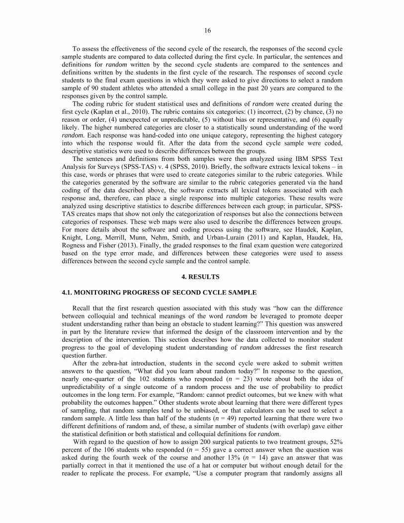
Understanding of random processes is a learning goal that is not specific to the teaching and learning of statistics. Genetic mutations studied in biological sciences, including molecular and cell biology, are random processes, as are radioactive decay and molecular collisions in physics and chemistry (Garvin-Doxas & Klymkowsky, 2008). At the end of a genetics class, students are typically expected to know and be able to write a sentence explaining that the three random processes that contribute to evolutionary processes are natural selection, speciation, and genetic drift (Garvin-Doxas & Klymkowsky, 2008). If, however, as previous research has shown (Kaplan et al., 2010), students persist in thinking that random processes are haphazard, weird or have unlikely outcomes, what might those students understand about the process of evolution? It seems reasonable to assume that the focus on the meaning of the word random and random processes within instruction in statistics classes will not only help student learning in statistics, but also learning in other STEM (science, technology, engineering, mathematics) disciplines. The latter provides a possible future direction for this research, which is discussed in Section 5.

3. RESEARCH METHODS

The study was designed using action research principles defined in Section 1. The remainder of this section describes the first three parts of the action research cycle.

3.1. DEFINITION OF THE PROBLEM

This paper describes the second cycle of action research associated with the lexical ambiguity

project focused on the word random. The first research cycle was motivated by the third author’s experience with students answering the exam question “How would you randomly select a sample of five gas stations in our town?” with responses such as, “Drive all over town and just randomly stop at 5 stations.” Results of the first cycle, which can be read in detail in Kaplan et al. (2010), were based on sentences and definitions written by students at three universities in the U.S. for the word random as used in the statistical sense. In summary, the findings of the first cycle of research were that only 8% of students included the idea of probability in their definition of random and that many of the students defined random as something without order or pattern (39%) or producing a representative or unbiased sample (23%). The sentences and definitions collected during the first cycle of action research will be discussed in more detail below and these data will be called the first cycle sample. In addition, prior to the analysis of the first cycle sample the first author included a question on a course final exam asking students to describe a method for selecting a random sample of 90 student athletes who matriculated in a small college over the past 20 years. The student responses were similar to those reported by the third author. In the detailed discussion below, these responses will be called the control sample. The findings from the first cycle and control samples prompted the research team to define the two research questions that are the focus of the second cycle of the action research and of this paper – to design and implement a classroom intervention in order to find out whether leveraging the ambiguity associated with the word random in the classroom would lead to better understanding of random and random processes by the students in the class.

3.2. DATA COLLECTION

Setting of the second cycle The intervention associated with the second cycle of the action research project was implemented in a one-semester introductory statistics course taught by the first author at a large research university in the Midwestern United States. The students in this course comprise what will be called the second cycle sample for the remainder of the paper. For three hours each week during a 15-week semester, the students met in lecture halls with approximately 120 students per lecture. The students attended an additional hour of recitation with a graduate teaching assistant once per week in classes of 30 students. The course was a three-credit algebra-based introduction to statistics course. It was a service course for non-majors and the “catch-all” course for

13

students since the department also offered introductory courses specifically for certain majors, such as science, business and elementary education. The largest major represented by students was pre-nursing, but there were also a number of criminal justice, journalism, communications, and psychology majors in the course. The course fulfilled the university’s mathematics requirement. The material covered was, in this order: data collection (surveys, studies and simulations), data analysis for one or two categorical variables, data analysis for one quantitative variable, probability models (discrete random variables, normal, binomial and geometric models), sampling distributions, inference for one or two proportions and one or two means, and data analysis (but not inference) for bivariate data. The semester ended with a brief introduction to chi-squared tests. This course did not include the use of computer technology or computer labs.

Intervention during the second cycle Recall there are two guiding principles to the intervention:

(1) provide opportunities for instructors to contrast the colloquial meanings with the statistical meanings and monitor student progress and (2) focus on random processes, not outcomes of random processes, in instruction. In the second class meeting of the course, the instructor contrasted the statistical and colloquial meanings of random, first activating students colloquial definitions for random by asking students to choose the meaning of the word random in the sentence, “Sometimes I say random things.” from these choices: A. Haphazard, weird, out of the ordinary, B. Without order or pattern, C. Without prior knowledge, criteria or method, D. By chance, or E. Without bias.

Next, students were asked to make a similar choice based on the sentence, “A group of participants was selected at random for the survey.” and given the choices: A. The choice was unexpected or unpredictable, B. People were chosen without order or reason, C. The choice was fair, representative and/or without bias, D. People were chosen by chance, and E. The choices were based on probability and everyone had a chance of being chosen. The answer choices were created based on the most common answers given by students in the authors’ previous studies (Kaplan et al., 2009, 2010).

Following the activation activity, the instructor showed her students two pictures (Figures 1a and 1b). The first was of three people dressed in rainbow-striped zebra costumes on a street in Shanghai to represent the colloquial definition of random: something that is weird, haphazard, or out of the ordinary. The other was an upside-down hat to represent the statistical definition of random: where choices or outcomes are based on probability. This introduction provided the instructor with the zebra-versus-hat mnemonic image for random that she used during the rest of the semester to contrast the statistical and colloquial meanings of random.

Figure 1a. Random Zebras (Colloquial). Figure 1b. Random Hat (Statistical).

The introductory activity, the addition of the zebra-versus-hat mnemonic image for random and

the collection of student writing about random, comprised the biggest change in the instructor’s teaching from previous semesters. Most of the other activities associated with the intervention had been used by the instructor previously. For example, on the third day of lecture, the class completed the Gettysburg Address activity (https://www.causeweb.org/webinar/teaching/2010-08/2010-08.pptx). The Gettysburg Address activity is isomorphic to the Random Rectangles activity appearing in the text Activity Based Statistics (Schaefer, Gnandesikan, Watkins, & Witmer, 1996). Students were given a copy of the Gettysburg Address and asked to estimate, just by looking at the Address, the

14

mean length of the words in the Address. The students were then asked to select a “reasonable” sample of 10 words and find the mean length of the 10 words in their sample. Finally, the students were asked to select a random sample of 10 words, using the random integer function on their calculators, and find the mean length of the 10 words in the random sample. When the results of the three estimates were compared, students were urged to notice that the means generated by the judgment samples are higher than the means generated by the random samples. In addition, they were told the true mean word length, which is estimated reasonably well by both the original guesses and the random samples, but is overestimated by the judgment samples, because our eyes are drawn to longer words and overlook the one-letter words “a” and “I.” The instructor connected the hat image to the random integer function of the calculator by telling her students to imagine that the calculator had a hat that it used to choose the integers it produced.

A homework problem collected at the end of the third week of the semester asked students to design an experiment to investigate the use of high doses of Vitamin E on healing time of surgical incisions. The problem specifically asked students to discuss the role of randomization in the design. Because very few students explained how they would randomly assign the surgical patients to the two groups, the instructor could not use the responses to monitor whether students were making progress in understanding what constitutes a random process. In the following week of class, therefore, she asked the students to submit the answer to

Let’s say you have recruited 200 surgical patients to participate in the study. Describe a method for assigning the 200 patients to two groups, one that receives vitamin E and one that receives a placebo, that allows for a statistically valid comparison of the two groups.

After they had answered the question, the students were asked, via a “clicker” or Personal Response System (PRS), if their response had been something similar to “assign the 200 people randomly to two treatments,” which the authors consider a vague answer from which we cannot tell what a student understands about random and random processes. Students who answered “yes” to the clicker question were encouraged to answer the written question again with instructions to make their answers more explicit.

The textbook used in the course emphasizes checking conditions for inference as a necessary step in performing hypothesis tests and constructing confidence intervals. One of the conditions that must be checked is the use of random sampling or random assignment to provide independence. The unit on inference, taught during weeks 6-12 of the course, provided opportunities for the instructor to contrast the colloquial and statistical meanings of random and to focus on random processes. Instead of making a cursory check of the “random” condition in an example of inference, the instructor was mindful of giving examples of processes that were and were not random. While no data were collected as to how many times this occurred during the lectures, there were several instances in which students were asked via their clickers to classify sampling and assignment processes as meeting or not meeting the statistical standard of random. One important aspect of the zebra-hat image is that it provides an image for both the statistical meaning and the colloquial meaning of random. This allowed the instructors to provide examples of sampling and assignment that matched colloquial usage, but did not meet the statistical definition of random as well as examples that met the statistical definition, but not the colloquial one. This differs from the typical statistics course in which the focus would be on only whether an example met the statistical meaning of random.

Samples and measures During each of the classes in which the intervention was implemented, written data were collected from the students in the second cycle sample. This was done to monitor student progress and to inform the ongoing design of the action research. After the zebra-versus-hat introduction and the Gettysburg Address activity, students were asked to submit written answers to the question, “What did you learn about random today?” The written responses describing the randomization of the 200 patients to two groups were also collected.

The first cycle sample was a random sample of student responses from a larger data set of responses collected across three universities, fourteen instructors and two geographic regions of the United States (Kaplan et al., 2010) who provided sentences and definitions for the statistical use of random at the end of a one-semester introduction to statistics course. In order to compare the students in the second cycle sample to the baseline data collected from the first cycle sample, each student in the second cycle sample was asked, during the last week of class, to write a sentence and provide a

15

definition for the primary meaning of random in statistics. The wording of this question and timing of the data collection were identical to that done in the first cycle (Kaplan et al., 2010). There is no reason to believe that the second cycle sample is not comparable to the first cycle sample, particularly since responses from students from the first author’s institution were included in the data set from which the first cycle sample was selected.

The control sample is comprised of the students from the course taught by the first author in a previous semester with no intervention. Students in both the control sample and the second cycle sample were asked the same question on the course final exam: “Describe a method for selecting a random sample of 90 student athletes who matriculated in a small college over the past 20 years.” The control sample and the second cycle sample did not differ in any other measures, such as scores on the Comprehensive Assessment of Outcomes of an introductory Statistics class (CAOS) test, attendance, homework and exam scores; as such, there is no reason to believe that the second cycle sample is not comparable to the control sample. A total of 107 students in the second cycle gave consent to have their data used for research purposes. All 107 students took the final exam, but not all were present in class on each day that data were collected. Table 1 contains a brief description of each sample and the measures associated with each as well as the sample sizes for the measures collected.

3.3. DATA ANALYSIS

The student responses used to monitor students’ progress toward understanding of the statistical meaning of the word random were analyzed qualitatively using open coding of the responses to create categories of responses and then grouping the responses by category. These results, along with student questions and responses to clicker questions asked during lecture but not reported here, were analyzed using only descriptive methods, as their purpose was to provide the instructor with feedback to be used in subsequent classes.

Table 1. Descriptions of the samples and measures

Outcome Measure What did

you learn about

random today?

Describe randomization into treatment

groups

Sentences and definitions for

random

Describe selection of

random sample

Sample

Control Fall 2008 Taught by first author, no intervention

(n = 103)

First Cycle Fall 2008 Random sample of students from large data set (3 institutions, 14 instructors)

(n = 65)

Second Cycle Spring 2010 Taught by first author, with intervention

(n = 102) (n = 106) (n = 82) (n = 107)

16

To assess the effectiveness of the second cycle of the research, the responses of the second cycle sample students are compared to data collected during the first cycle. In particular, the sentences and definitions for random written by the second cycle students are compared to the sentences and definitions written by the students in the first cycle of the research. The responses of second cycle students to the final exam questions in which they were asked to give directions to select a random sample of 90 student athletes who attended a small college in the past 20 years are compared to the responses given by the control sample.

The coding rubric for student statistical uses and definitions of random were created during the first cycle (Kaplan et al., 2010). The rubric contains six categories: (1) incorrect, (2) by chance, (3) no reason or order, (4) unexpected or unpredictable, (5) without bias or representative, and (6) equally likely. The higher numbered categories are closer to a statistically sound understanding of the word random. Each response was hand-coded into one unique category, representing the highest category into which the response would fit. After the data from the second cycle sample were coded, descriptive statistics were used to describe differences between the groups.

The sentences and definitions from both samples were then analyzed using IBM SPSS Text Analysis for Surveys (SPSS-TAS) v. 4 (SPSS, 2010). Briefly, the software extracts lexical tokens – in this case, words or phrases that were used to create categories similar to the rubric categories. While the categories generated by the software are similar to the rubric categories generated via the hand coding of the data described above, the software extracts all lexical tokens associated with each response and, therefore, can place a single response into multiple categories. These results were analyzed using descriptive statistics to describe differences between each group; in particular, SPSS-TAS creates maps that show not only the categorization of responses but also the connections between categories of responses. These web maps were also used to describe the differences between groups. For more details about the software and coding process using the software, see Haudek, Kaplan, Knight, Long, Merrill, Munn, Nehm, Smith, and Urban-Lurain (2011) and Kaplan, Haudek, Ha, Rogness and Fisher (2013). Finally, the graded responses to the final exam question were categorized based on the type error made, and differences between these categories were used to assess differences between the second cycle sample and the control sample.

4. RESULTS

4.1. MONITORING PROGRESS OF SECOND CYCLE SAMPLE Recall that the first research question associated with this study was “how can the difference

between colloquial and technical meanings of the word random be leveraged to promote deeper student understanding rather than being an obstacle to student learning?” This question was answered in part by the literature review that informed the design of the classroom intervention and by the description of the intervention. This section describes how the data collected to monitor student progress to the goal of developing student understanding of random addresses the first research question further.

After the zebra-hat introduction, students in the second cycle were asked to submit written answers to the question, “What did you learn about random today?” In response to the question, nearly one-quarter of the 102 students who responded (n = 23) wrote about both the idea of unpredictability of a single outcome of a random process and the use of probability to predict outcomes in the long term. For example, “Random: cannot predict outcomes, but we knew with what probability the outcomes happen.” Other students wrote about learning that there were different types of sampling, that random samples tend to be unbiased, or that calculators can be used to select a random sample. A little less than half of the students (n = 49) reported learning that there were two different definitions of random and, of these, a similar number of students (with overlap) gave either the statistical definition or both statistical and colloquial definitions for random.

With regard to the question of how to assign 200 surgical patients to two treatment groups, 52% percent of the 106 students who responded (n = 55) gave a correct answer when the question was asked during the fourth week of the course and another 13% (n = 14) gave an answer that was partially correct in that it mentioned the use of a hat or computer but without enough detail for the reader to replicate the process. For example, “Use a computer program that randomly assigns all

17

patients to a group.” Nineteen percent of the students (n = 20) gave the vague answer of “use random assignment” to start and half of those were able to give a correct response to the follow-up question. Eight percent of the students (n = 9) mentioned stratifying or blocking (e.g., by gender or surgery type). By the end of the activity, 68% of students (n = 72) had provided a correct description of a randomization process.

While it is clear from the data that not every student was successful at mastering the ability to recognize and describe methods of random and nonrandom sampling, there is evidence in the data that the class, as a whole, was making progress on these learning outcomes. In the first week of class only about half of the students were able to write coherently about the statistical meaning of the word random. By the middle of the semester two-thirds of the students were making reasonable progress toward the goal of developing understanding of random and random processes, as evidenced by the results on the question of random assignment of patients to treatment groups.

4.2. COMPARISON OF FIRST CYCLE AND SECOND CYCLE SAMPLES

This section describes the results with regard to the second research question: What are the

differences in the knowledge exhibited by students who experienced the intervention when compared with students who did not experience the intervention?

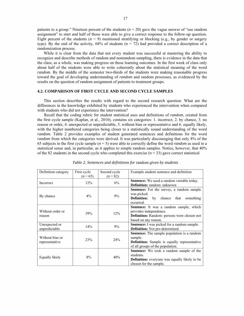
Recall that the coding rubric for student statistical uses and definitions of random, created from the first cycle sample (Kaplan, et al., 2010), contains six categories: 1. incorrect, 2. by chance, 3. no reason or order, 4. unexpected or unpredictable, 5. without bias or representative and 6. equally likely, with the higher numbered categories being closer to a statistically sound understanding of the word random. Table 2 provides examples of student generated sentences and definitions for the word random from which the categories were derived. It was particularly discouraging that only 8% of the 65 subjects in the first cycle sample (n = 5) were able to correctly define the word random as used in a statistical sense and, in particular, as it applies to simple random samples. Notice, however, that 40% of the 82 students in the second cycle who completed this exercise (n = 33) gave correct statistical

Table 2. Sentences and definitions for random given by students

Definition category First cycle

(n = 65) Second cycle

(n = 82) Example student sentence and definition

Incorrect 12% 6% Sentence: We used a random variable today. Definition: random: unknown

By chance 4% 9%

Sentence: For the survey, a random sample was picked. Definition: by chance that something occurred.

Without order or reason

39% 12%

Sentence: It was a random sample, which provides independence. Definition: Random: persons were chosen not based on any reason.

Unexpected or unpredictable

14% 9% Sentence: I was picked for a random sample. Definition: Not pre-determined.

Without bias or representative

23% 24%

Sentence: The sample population is a random sample. Definition: Sample is equally representative of all groups of the population.

Equally likely 8% 40%

Sentence: We took a random sample of the students. Definition: everyone was equally likely to be chosen for the sample.

18

definitions. In contrast to the first cycle sample, the second cycle student responses are clustered toward the bottom of the table, which represents uses and definitions that are closer to the correct statistical use of the word random.

Similar results are seen in Figure 2, which shows the results of the SPSS-TAS analysis of the data. The first set of bars shows the percent of students in each sample who used the phrase random sample in their response. The next 5 sets of bars represent the five categories derived from the hand coding (the incorrect category cannot be derived from the software), shown in the same order, left to right, as appears top to bottom in Table 2. Notice a similar pattern to the bars as was seen in Table 2, with data concentrating in the categories corresponding more to the statistical meanings of random. Finally, notice that the word probability, which was extracted as a lexical token, was not used at all by the students in the first cycle sample, but did appear in the sample collected from the second cycle. It is disappointing that none of the responses in the first cycle sample contained the word probability. Another word that appeared in the second cycle sample data, but not in the first cycle sample data, was hat, which prompted the researchers to search for other random agents, such as computer or coin. Only one student in the first cycle had mentioned an agent (computer). In contrast, 30% of the second cycle students mentioned an agent and 19 of the 25 mentions were of a hat. This indicates that the zebra-versus-hat mnemonic image was something with which the students connected and were accessing to understand the statistical idea of random.

Figure 2. Categorization by SPSS-TAS software.

The SPSS-TAS software can also create webmaps (see Figures 3 and 4) of the extracted categories and tokens. This shows not only the ideas and phrases present in the responses, but also the connections among the categories that tend to appear in the data. The webmaps include nodes (the circles) for each category or lexical token. The size of the node is proportional to the number of responses. Since the largest node for the first cycle sample was random sample, it was the category into which the largest number of responses was placed. Similarly the largest nodes for the second cycle sample were random sample and equal chance. The thickness of the line that connects two nodes indicates the number of responses that include both of the connected tokens. In particular, webmaps that include the five original rubric coding categories along with a category for the phrase random sample and a category for the mention of an agent of randomness, such as a coin, die or hat, were created.

The webmaps show additional differences between the second cycle students and the first cycle sample in their writing about random. In the first cycle sample webmap (Figure 3), the strongest connections (denoted by the thickest lines) are between the three categories of 1. random sample, 2. without bias or representative and 3. no reason or order. In contrast, the strong connections on the

0%

10%

20%

30%

40%

50%

60%

PercentofSam

ple

FirstCycle(n=65)

SecondCycle(n=82)

19

second cycle webmap (Figure 4) include random sample, equal chance, and agents. The thick connecting lines on the second cycle webmap include the statistical ideas underlying random, whereas the first cycle webmap connections reflect a more colloquial use of random. Furthermore, the position of the category agents is markedly different in the two webmaps. In the first cycle sample data, only the students whose responses were in the unpredictable category also mention agents. In contrast, the category agents in the second cycle sample responses is well connected to all of the other categories. This indicates further the value of the hat image even for students who are still struggling to understand the concept of statistical randomness.

Figure 3. Webmap of definitions of random by the first cycle sample.

Figure 4. Webmap of definitions of random by the second cycle sample.

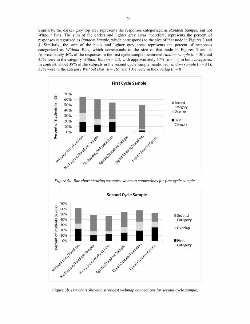
These differences can also be seen in Figures 5a and 5b, in which the major connections in the webmaps (Figures 3 and 4) have been converted into bars. Each bar represents a coupling of two phrases. For example, the leftmost bar on each panel in Figures 5a and 5b represents the two nodes and connection between the categories Without Bias and Random Sample from the webmaps in Figures 3 and 4. The lightest area (in the center) represents the percent of subjects who mentioned both phrases in their responses. This area, therefore, corresponds to the width of the connector between the two nodes and shows the strength of the connection between the two phrases. The bottom black area represents the percent of all responses categorized as Without Bias but not Random Sample.

20

Similarly, the darker grey top area represents the responses categorized as Random Sample, but not Without Bias. The sum of the darker and lighter grey areas, therefore, represents the percent of responses categorized as Random Sample, which corresponds to the size of that node in Figures 3 and 4. Similarly, the sum of the black and lighter grey areas represents the percent of responses categorized as Without Bias, which corresponds to the size of that node in Figures 3 and 4. Approximately 46% of the responses in the first cycle sample mentioned random sample (n = 30) and 35% were in the category Without Bias (n = 23), with approximately 17% (n = 11) in both categories. In contrast, about 38% of the subjects in the second cycle sample mentioned random sample (n = 31), 32% were in the category Without Bias (n = 26), and 10% were in the overlap (n = 8).

Figure 5a. Bar chart showing strongest webmap connections for first cycle sample.

Figure 5b. Bar chart showing strongest webmap connections for second cycle sample.

0%10%20%30%40%50%60%70%

Percent of Students (n = 65)

First Cycle Sample

SecondCategoryOverlap

FirstCategory

0%

10%

20%

30%

40%

50%

60%

70%

Percent of Students (n = 82)

Second Cycle Sample

SecondCategory

Overlap

FirstCategory

21

In summary, the left three bars on panel of Figure 5a and 5b represent the percent of students who

connected the three categories, Random Sample, Without Bias or Representative, and No Reason or Order. The rightmost three bars represent the connections between three categories of Equal Chance, Agents, and Random Sample. Notice that the first set of connections appears in both data sets, though with relatively fewer mentions of No Reason or Order in the second cycle sample. Notice also that the only connections made between more statistical meanings of random in the first cycle sample were between Random Sample and Equal Chance and those were made by very few students. In contrast, there are more robust connections between the statistical meanings evident in the second cycle sample.

4.3. COMPARISION OF THE SECOND CYCLE AND CONTROL SAMPLES

Recall the question on the final exam in which students were asked to give directions to select a

random sample of 90 student athletes who attended a small college in the past 20 years. This question had been given to students in the control sample, the class taught by the first author, in the semester before the intervention was implemented. This question was repeated on the final exam given to the students in the second cycle sample. Forty-three percent of the 103 students in the control sample (n = 44) gave a valid statistical response to the problem, suggesting that names be drawn out of a hat or that random numbers be generated and used to select from an ordered list. In contrast, 78% of the 107 students in the second cycle sample (n = 83) gave a valid statistical answer to the question. An additional 12% of students in the second cycle sample (compared to 7% of the control sample) suggested the use of a computer program but without specifying in what way. Finally, fewer than 3% of the second cycle sample suggested that the athletes be stratified across gender, sport, or year, as compared to 16% of the control sample, suggesting that the students in the second cycle sample had learned that random samples are representative by nature, rather than by having to incorporate stratification into the design.

5. DISCUSSION

5.1. IMPLICATION OF THE RESULTS FOR TEACHING

This paper reports the results of a second cycle of action research associated with a project

designed to address issues in student learning of statistics associated with the lexical ambiguity of the statistical term random. In the first cycle of the research, the researchers found that students do not develop strong understandings of the statistical meaning of the word random (Kaplan et al., 2010). In the second cycle of the research, the authors designed and tested a classroom intervention based on the literature about issues associated with people’s understanding of random processes and the literature on lexical ambiguity. A key feature of the intervention was the use of the zebra-versus-hat mnemonic image that provides a mental picture for students of both what is and what is not classified as random in the statistical sense. Most introductory statistics courses, instructors and texts provide examples and definitions for random as a technical word in statistics. The innovation in this intervention is the inclusion of examples of phenomena that statisticians do not consider to be random, thus contrasting the colloquial and statistical definitions of the words.

The literature review described in Section 2 and subsequent design of the intervention described in Section 3.2 provide a theoretical answer to the first research question posed: how can the ambiguity associated with the word random be leveraged to promote student learning? The results described in Section 4 provide an answer to the second research question: What are the differences in the knowledge exhibited by students who experience the intervention? In particular, the students in the second cycle sample wrote definitions for the word random that showed more similarities to the statistical definition than were found in the first cycle sample. Furthermore, the second cycle students tended to have more connections between the concepts that underlie random processes as evidenced by the number of connections present in the webmap for these students. Finally, the students in the second cycle performed better on a test of knowledge of random sampling than did the students in the control sample. We therefore suggest as a result of this research that instructors consider using

22

examples and counterexamples of events that are and events that are not statistically random, finding opportunities throughout the semester to monitor students’ progress toward the goal of understanding the technical meaning of random. 5.2. LIMITATIONS AND DELIMITATIONS

Study limitations stem from issues of internal validity while delimitations are the results of issues related to external validity, or generalizability (Dereshiwsky, 1999). This study did not attempt to assign students randomly to treatments. It is an observational study in which all of the second cycle students are nested within one class (and one instructor). These factors are limitations of the study because the observed differences between subjects cannot be attributed directly to the intervention. They are, in fact, confounded with class and instructor variables.

The study does attempt to use large samples that represent the entire population where possible. The first cycle sample, as a random sample of students across multiple instructors at three institutions in two states, can arguably be viewed as a random sample of university students in introductory statistics courses. The second cycle students, however, are not a random sample and are nested within the same class. These individuals are not independent from one another, attending the same university, having the same lectures from the same instructor, and using the same textbook. A delimitation of this study, therefore, is that the findings may not be generalizable to other populations, even populations of undergraduate students at similar universities. 5.3. DIRECTIONS FOR FUTURE RESEARCH

The results of the classroom intervention during the second cycle suggest, as a proof of concept, that providing students with an analogy, such as the zebra-versus-hat mnemonic image, which contrasts the statistical and colloquial meanings of random providing both examples and counter-examples, along with continued attention during instruction that emphasizes random processes rather than outcomes is effective in helping students develop deeper understandings of random. There is, however, much more work to be done both on the general issue of addressing lexical ambiguity in statistics and in the particular case of developing deeper student understanding of the word random and associated random processes. These data do not provide evidence about the mechanisms by which the changes are occurring. That is, we do not know why or how the changes occurred. We therefore also do not know which aspects of the intervention were successful and which were superfluous. We do not know how faithful an instructor must be to the described intervention to produce similar results in other classes, nor do we know which aspects should be enhanced to increase the learning on the part of the students.

Clearly, richer data should be collected to investigate the issues raised above. Fidelity issues could be addressed by collecting audio data from classrooms in which other instructors are attempting to implement the intervention. Students of these instructors could be interviewed over the course of the semester using some of the same questions used in the intervention to probe student understandings and misunderstandings of random. Through interviews, researchers would learn why systematic samples are thought by some students to be equivalent to random samples or why students think that stratification is a necessary step in taking a random sample. Furthermore, there is the opportunity for statistics education researchers to work with researchers in evolutionary biology education to answer similar research questions. As mentioned in the literature review, a typical sentence that might appear in an evolution textbook or be a correct response to a test questions is, “Three random events that will contribute to evolutionary processes are natural selection, speciation, and genetic drift” (Garvin-Doxas & Klymkowsky, 2008, p. 230). One possible research question is, in the previous sentence, how do students interpret the meaning of random? Results of such a study could be used to design interventions that target student understanding of random processes that can be implemented in other science disciplines.

The promising results of the intervention for random suggests a continuation of this work with other words found to exhibit lexical ambiguity (Kaplan et al., 2009). Based on the data collected in the second cycle, it was suggested that the use of spread as the primary word when instructors mean variability be discontinued (Kaplan, Rogness, & Fisher, 2012). Two other words of interest are

23

average and normal. Because the second cycle sample students tended to give normal as a colloquial synonym for average, contrasting the meanings of average and normal during instruction (as suggested by Utts, 2005) has the potential to increase student learning in much the same way that focusing on random processes and contrasting the colloquial and statistical meanings of random has been shown to do.

ACKNOWLEDGMENTS

The authors thank the Automated Analysis of Constructed Response (AACR) research group for

connecting the Lexical Ambiguity research group with the available software. In particular, Kevin Haudek was instrumental in providing the results of the data analysis. A big thank you goes to Nicole Ellefson who not only took the photograph of the random zebras, but posted it to Facebook and gave us permission to use it in our research. The authors also thank Dianne Cook for her suggestions about displaying the results and John Gabrosek for his careful reading of our near-final draft of the paper. In addition, the authors are grateful for the comments made by the two anonymous reviewers and the associate editor. These comments were invaluable for providing an organizational framework for the paper. Any errors or issues, however, are solely the responsibility of the authors and not their helpers.

REFERENCES

Adams, T. L., Thangata, F., & King, C. (2005). ‘Weigh’ to go: Exploring mathematical language.

Mathematics Teaching in the Middle School, 10(9), 444–448. Albert, J. H. (2003). College students’ conceptions of probability. The American Statistician, 57(1),

37–45. Barwell, R. (2005). Ambiguity in the mathematics classroom. Language and Education, 19(2), 118–

126. Batanero, C., Godino, J. D., & Roa, R. (2004). Training teachers to teach probability. Journal of

Statistics Education, 12(1). [ Online: http://www.amstat.org/publications/jse/v12n1/batanero.html ]

Batanero, C., & Serrano. L. (1999). The meaning of randomness for secondary school students. Journal for Research in Mathematics Education, 30(5), 558–567.

Dereshiwsky, M. (1999). Limitations and delimitations [electronic textbook]. Flagstaff, AZ: Northern Arizona University. [ Online: http://jan.ucc.nau.edu/~mid/edr720/class/methodology/delimitations/ ]

Durkin, K., & Shire, B. (1991a). Lexical ambiguity in mathematical contexts. In K. Durkin & B. Shire (Eds.), Language in mathematical education: Research and practice (pp. 71–84). Philadelphia, PA: Open University Press.

Durkin, K., & Shire, B. (1991b). Primary school children’s interpretations of lexical ambiguity in mathematical descriptions. Journal of Research in Reading, 14(1), 46–55.

Falk, R. (1991). Randomness – an ill-defined but much needed concept. Journal of Behavioral Decision Making, 4(3), 215–218.

Garvin-Doxas, K., & Klymkowsky, M. W. (2008). Understanding randomness and its impact on student learning: Lessons learned from building the Biology Concept Inventory (BCI). CBE Life Sciences Education, 7(2), 227–233.

Hahn, U., & Warren, P. A. (2009). Perceptions of randomness: Why three heads are better than four. Psychological Review, 116(2), 454–461.

Haudek, K. C., Kaplan, J. J., Knight, J., Long, T., Merrill, J., Munn, A., Nehm, R., Smith, M., & Urban-Lurain, M. (2011). Harnessing technology to improve formative assessment of student conceptions in STEM: Forging a national network. CBE – Life Sciences Education, 10(2), 149–155. [ Online: http://www.lifescied.org/cgi/reprint/10/2/149 ]

Hyland, K., & Tse, P. (2007). Is there an “academic vocabulary”? TESOL Quarterly 41(2), 235–252. Johnson, A. P. (2012). A short guide to action research (4th ed.). Upper Saddle River, NJ: Pearson

Education, Inc.

24

Kaplan, J. J., Haudek, K. C., Ha, M., Rogness, N., & Fisher, D. (2013). Using lexical analysis software to assess student writing in statistics. Manuscript submitted for publication.

Kaplan, J. J., Fisher, D., & Rogness, N. (2009). Lexical ambiguity in statistics: What do students know about the words: association, average, confidence, random and spread? Journal of Statistics Education, 17(3), 1–19. [ Online: http://www.amstat.org/publications/jse/v17n3/kaplan.pdf ]

Kaplan, J. J., Fisher, D., & Rogness, N. (2010). Lexical ambiguity in statistics: How students use and define the words: association, average, confidence, random and spread. Journal of Statistics Education, 18(2), 1–22. [ Online: http://www.amstat.org/publications/jse/v18n2/kaplan.pdf ]

Kaplan, J. J., Rogness, N., & Fisher, D. (2012). Lexical ambiguity: Making a case against spread. Teaching Statistics, 34(2), 56–60.

Lavy, I., & Mashiach-Eizenberg, M. (2009). The interplay between spoken language and informal definitions of statistical concepts. Journal of Statistics Education, 17(1), 1–9. [ Online: http://www.amstat.org/publications/jse/v17n1/lavy.pdf ]

Lecoutre M.-P., Rovira K., Lecoutre, B., & Poitevineau J. (2006). People’s intuitions about randomness and probability: An empirical study. Statistics Education Research Journal, 5(1), 20–35. [ Online: http://iase-web.org/documents/SERJ/SERJ_5(1)_Lecoutre_Rovira_Lecoutre_Poitevineau.pdf ]

Lemke, J. (1990). Talking science: Language, learning and values. Norwood, NJ: Ablex Publishing Corporation.

Makar, K., & Confrey, J. (2005). “Variation-talk”: Articulating meaning in statistics. Statistics Education Research Journal, 4(1), 27–54. [ Online: http://iase-web.org/documents/SERJ/SERJ4(1)_Makar_Confrey.pdf ]

Moore, D. (2007). The basic practice of statistics (4th ed.). New York: W. H. Freeman and Company. Ochs, T. L. (1990). Nonrandom uses. Nature, 343(6246), 303. Pinker, S. (1994). The language instinct: How the mind creates language. New York: HarperCollins

Publisher. Rangecroft, M. (2002). The language of statistics. Teaching Statistics, 24(2), 34–37. Schaeffer, R. L., Gnanadesikan, M., Watkins, A., & Witmer, J. A. (1996). Activity-based statistics.

New York: Springer-Verlag. Shultz, T., & Pilon, R. (1973). Development of the ability to detect linguistic ambiguity. Child

Development, 44(4), 728–733. SPSS (2010). SPSS text analytics for surveys 4.0 user’s guide, Chicago, IL: SPSS, Inc. Thompson, D., & Rubenstein, R. (2000). Learning mathematics vocabulary: Potential pitfalls and

instructional strategies. Mathematics Teacher, 93(7), 568–574. Utts, J. M. (2005). Seeing through statistics (3rd ed.). Belmont, CA: Thompson Brooks/Cole. Wagenaar, W. (1991). Randomness and randomizers: Maybe the problem is not so big. Journal of

Behavioral Decision Making, 4(3), 220–222.

JENNIFER J. KAPLAN Department of Statistics

University of Georgia Athens, GA 30602 USA