Embed Size (px)
Citation preview

Explicit Treatment of Model ErrorSimultaneous State and Parameter
Estimation with an Ensemble Kalman Filter
Altuğ Aksoy*, Fuqing Zhang, and John W. Nielsen-Gammon
Texas A&M University
* Current affiliation: National Center for Atmospheric Research
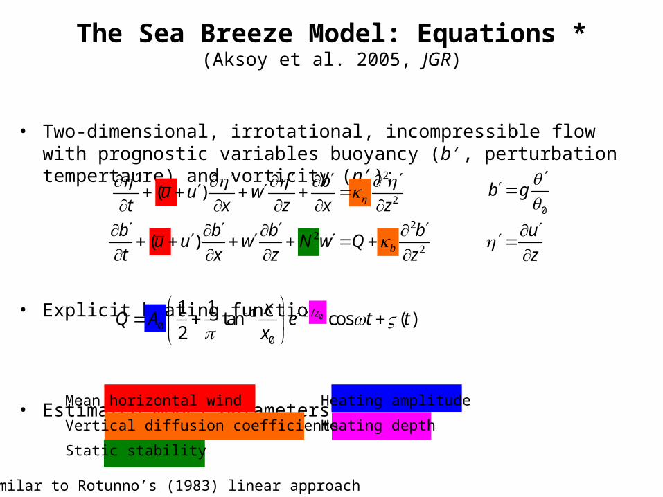
• Two-dimensional, irrotational, incompressible flow with prognostic variables buoyancy (b′, perturbation tempertaure) and vorticity (η′):
• Explicit heating function:
• Estimated model parameters:
0/10
0
1 1tan cos ( )
2z zx
Q A e t tx
2
2
22
2
( )
( ) b
bu u w
t x z x z
b b b bu u w N w Q
t x z z
Mean horizontal wind
Vertical diffusion coefficients
Static stability
Heating amplitude
Heating depth
The Sea Breeze Model: Equations *(Aksoy et al. 2005, JGR)
0
b g
u
z
* Similar to Rotunno’s (1983) linear approach
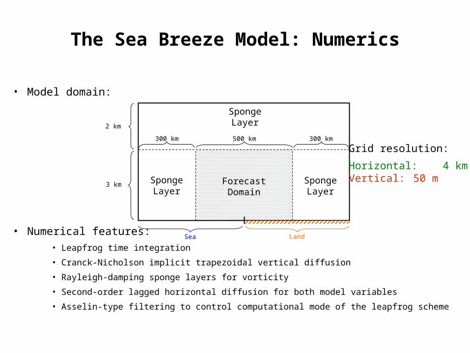
The Sea Breeze Model: Numerics
• Model domain:
• Numerical features:• Leapfrog time integration
• Cranck-Nicholson implicit trapezoidal vertical diffusion
• Rayleigh-damping sponge layers for vorticity
• Second-order lagged horizontal diffusion for both model variables
• Asselin-type filtering to control computational mode of the leapfrog scheme
LandSea
ForecastDomain
SpongeLayer
SpongeLayer
SpongeLayer
500 km300 km 300 km
Grid resolution:
Horizontal: 4 kmVertical: 50 m
2 km
3 km

The Sea Breeze Model: Perfect-model behavior
LandSea
LandSea
Winds and Streamfunction
VorticityTemperature
LandSea
48H Forecast
NoonMaximumHeating
3 km 3 km
3 km
Surface Surface
Surface
250 km 500 km 250 km 500 km
250 km 500 km

LandSea
LandSeaLandSea
51H Forecast
3:00PMOnset of
Sea Breeze
Temperature Vorticity
Winds and Streamfunction
3 km 3 km
3 km
Surface Surface
Surface
250 km 500 km 250 km 500 km
250 km 500 km
The Sea Breeze Model: Perfect-model behavior

LandSea
LandSea
Winds and Streamfunction
Vorticity
LandSea
54H Forecast
6:00PMWarmest
Temperature
Temperature3 km 3 km
3 km
Surface Surface
Surface
250 km 500 km 250 km 500 km
250 km 500 km
The Sea Breeze Model: Perfect-model behavior

LandSea
LandSea
Winds and Streamfunction
Vorticity
LandSea
57H Forecast
9:00PMStrongest
Sea Breeze
Temperature3 km 3 km
3 km
Surface Surface
Surface
250 km 500 km 250 km 500 km
250 km 500 km
The Sea Breeze Model: Perfect-model behavior

LandSea
LandSea
Winds and Streamfunction
Vorticity
LandSea
60H Forecast
MidnightMaximumCooling
Temperature3 km 3 km
3 km
Surface Surface
Surface
250 km 500 km 250 km 500 km
250 km 500 km
The Sea Breeze Model: Perfect-model behavior

LandSea
LandSea
Winds and Streamfunction
Vorticity
LandSea
63H Forecast
3:00AMOnset of
Land Breeze
Temperature3 km 3 km
3 km
Surface Surface
Surface
250 km 500 km 250 km 500 km
250 km 500 km
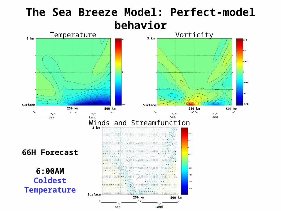
The Sea Breeze Model: Perfect-model behavior
LandSea
LandSea
Winds and Streamfunction
Vorticity
LandSea
66H Forecast
6:00AMColdest
Temperature
Temperature3 km 3 km
3 km
Surface Surface
Surface
250 km 500 km 250 km 500 km
250 km 500 km
The Sea Breeze Model: Perfect-model behavior

LandSea
LandSea
Winds and Streamfunction
Vorticity
LandSea
69H Forecast
9:00AMStrongest
Land Breeze
Temperature3 km 3 km
3 km
Surface Surface
Surface
250 km 500 km 250 km 500 km
250 km 500 km
The Sea Breeze Model: Perfect-model behavior

LandSea
LandSea
Winds and Streamfunction
Vorticity
LandSea
72H Forecast
NoonMaximumHeating
Temperature3 km 3 km
3 km
Surface Surface
Surface
250 km 500 km 250 km 500 km
250 km 500 km
The Sea Breeze Model: Perfect-model behavior

Model Error - Enkf Properties (Aksoy et al. 2006, MWR)
• Observations: Surface buoyancy observations on land
• Observational error: Standard deviation of 10-3 ms-2
• Observation spacing: 40 km (10 grid points)
• Ensemble size: 50 members
• Ensemble initialization: Perturbations from model climatology
• Covariance localization: Gaspari and Cohn’s (1999) fifth-order correlation function with 100
grid-point radius of influence
• Observation processing: Sequential with no correlation between observation errors (Snyder and Zhang 2003)
• Filter: Square-root after Whitaker and Hamill (2002) with no perturbed observations

Bu
oya
ncy
Vo
rtic
ity
3H Prior
3H Prior
3H Posterior
3H Posterior
Perfect-Model EnKF Results
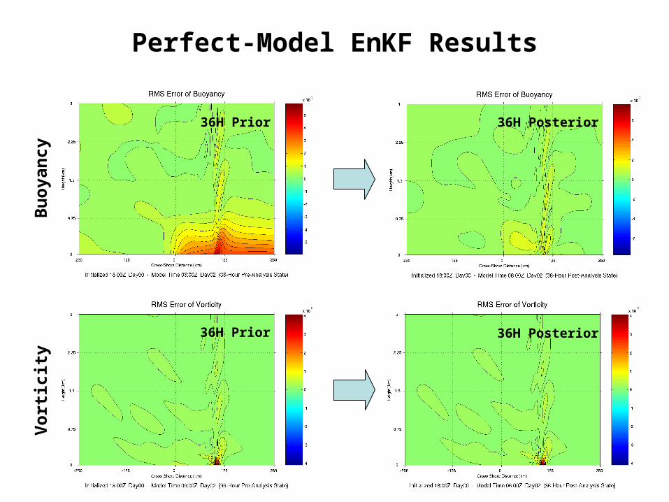
Bu
oya
ncy
Vo
rtic
ity
36H Prior
36H Prior
36H Posterior
36H Posterior
Perfect-Model EnKF Results
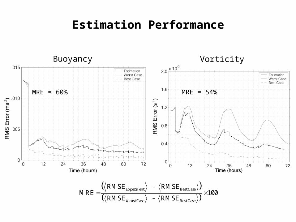
Estimation Performance
Buoyancy Vorticity
Experiment Best Case
Worst Case Best Case
RMSE - RMSEMRE 100
RMSE - RMSE
MRE = 60% MRE = 54%

Estimation Performance
Mean horizontal wind Static stability Vorticity diff. coef.
Buoyancy diff. coef. Heating amplitude Heating depth
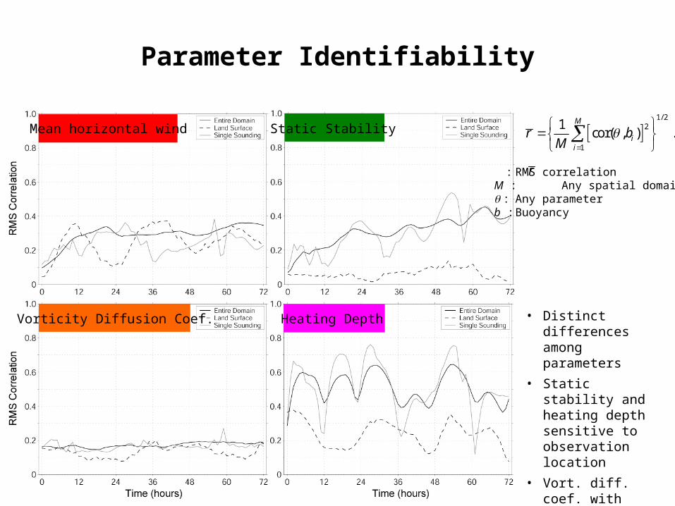
Mean horizontal wind
Parameter Identifiability
1/ 2
2
1
1cor( , ) .
M
ii
r bM
Static Stability
Vorticity Diffusion Coef. Heating Depth
: RMS correlationM : Any spatial domain : Any parameterb : Buoyancy
r
• Distinct differences among parameters
• Static stability and heating depth sensitive to observation location
• Vort. diff. coef. with smallest correlation, appears to exhibit smallest identifiability

MM5 Experiments: Experimental Setup (Aksoy et al. 2006, GRL, submitted)
• 36-km resolution with55×55 grid-point domain
• 43 vertical sigma layers with50 hPa model top
• Initialized: 00Z 28 Aug 2000
• Parameterizations:• MRF PBL scheme
• Grell cumulus scheme withshallow cumulus option
• Simple-ice microphysicalparameterization
• Prognostic variables• Winds (u, v, w )
• Temperature (T )
• Water vapor mixing ratio (q )
• Pressure perturbation (p ‘ )

Control Forecast
•Evidence of the clockwise turning of winds
•Penetration of the temperature and moisture gradients inland during the sea breeze phase
•Well-established return flow during the land breeze phase
Sea breeze phase (7pm local)
Land breeze phase

Ensemble and Filter Properties
• Ensemble size: 40 members
• Observations: Surface and sounding observations of u, v, and T
• Observational error: Std. deviations of 2 ms-1 for u and v ; 1 K for T
• Observation spacing: 72 km for surface, 324 km for sounding
• Covariance localization: Gaspari and Cohn’s (1999) fifth-order correlation function with 30 grid-
point radius of influence
• Observation processing: Sequential (Snyder and Zhang 2003)
• Filter: Square-root (Whitaker and Hamill 2002)
Parameter Estimation Details
• Not attempting to identify individual error sources within the PBL scheme associated with different empirical parameters:
– Multiplier (m) of the vertical eddy mixing coefficient implanted into the MRF PBL code → for a value of 1.0, the original MRF PBL computation is simply repeated
• Variance limit applied at 1/4 of initial parameter error
• Updating is carried out spatially:
– Prior parameter value converted to 2-d matrix assumed at surface
– Spatial updating is performed with same covariance localization properties as the updating of the state
– Updated 2-d distribution is averaged to obtain posterior global parameter value

Correlation Signal – (T,m) and (U,m)
•Relatively strong overall correlation signal with both temperature and winds (signal strength “comparable” to idealized sea breeze model experiments)
•Spatially and temporally varying correlation structure
•Stronger signal near the surface
•Smaller-scale variability with horizontal winds

Estimation Performance – 3 CasesInitial Mean Error = +0.2 Initial Mean Error = +0.65 Initial Mean Error = -0.3

Concluding Remarks
• EnKF demonstrated to be promising for explicit treatment of model error through simultaneous state and parameter estimation
• Lessons from the idealized sea breeze model experiments:
– Sensitivity to observation location, radius of influence, and variance limit is parameter-specific
– Counter-acting correlations do lead to identifiability issues with some parameter pairs (do we really need to estimate every single parameter?)
• A more global approach to the MRF PBL scheme in MM5 appears to be responding well
• Updating of a global parameter through observations that contain spatial information is an issue and does lead to divergence as number of observations increases:
– We have approached this problem through our “spatial updating” technique – ad hoc but effective