Explaining model’s visual explanations from itsdecision

Dipesh TamboliIndian Institute of Technology Bombay, Mumbai, India

dipesh.tamboli@gmail.com

Abstract—This document summarizes different visual expla-nations methods such as {CAM, Grad-CAM, Localization usingMultiple Instance Learning} - Saliency based methods, {Saliencydriven Class-Impressions, Muting pixels in input image} - Adver-sarial methods as well as {Activation visualization, Convolutionfilter visualization} - Feature-based methods. We have also shownthe results produced by different methods as well as a comparisonbetween CAM, GradCAM and Guided Backpropagation.

Index Terms—visualization, explanations, features, saliencymaps

I. INTRODUCTION

In recent years, Deep Neural Networks has shown im-pressive classification performance on a huge dataset suchas Imagenet. Deep Learning regime empowers classifiers toextract distinct patterns of a given class from training data,which is the basis on which they generalize to unseen data.However, our understanding of how these models work or whythey perform so well is not very clear. Before deploying thesemodels on critical applications such as Medical Image Anal-ysis, Road-Lane-Traffic light detection, etc., it is necessary tovisualize the features considered to be important for makingthe decision.

There are several methods to generate visual explanationsfor a trained model. Saliency based methods first forward prop-agate the image and used the activation signal corresponding tothe target class only for the backpropagation to the differentlayers of the network. These backpropagated gradient mapsare combined differently to produce heatmaps to show thevisualization.

In the data-free saliency approach(Addepalli et al., 2020),noise is adversarially modified to maximize the confidence ofthe target class, which transforms it into the picture whichmodel has in its memory. Muting the pixels in the inputimage and generating the heatmap from the confidence of thetarget class highlights the location where an important objectis present in the image.

Feature-based methods use weights of themodel(specifically of convolution filter’s) to conclude it.Zeiler and Fergus have shown that those filters resemble theGabor filters.

The organization of this document is briefly described here.In the following section, we described related literature inthe field of Visualization of Deep Networks and showed their

results. Section-III describes the project idea and explains thecode. We conclude the paper with our analysis in Section-IV.

II. DIFFERENT METHODS

A. Visualizing Live ConvNET Activations

For visualizing what convolutional filters have learnt,(Yosinski et al., 2015) has plotted the activation value ofneurons directly in response to an image or video. As inconvolutional network, filters are applied in a way that respectsthe underlying geometry of the input. But that’s not the casefor the fully connected network as the order of the units isirrelevant. Thus this method is useful only for visualizing thefeatures of the convolutional network.

In the Fig.1, the activation of a conv5 filter is shown whichis trained on the Imagenet dataset. The point to be noted hereis that the Imagenet dataset has no specific class for Face, butstill, the model can capture it as an important feature for theclassification.

B. Saliency-Driven Class Impressions

In this input-agnostic data-free method (Addepalli et al.,2020) has proposed a method of generating visualizationscontaining highly discriminative features learned by the net-work. They initially start with a noise image and iterativelyupdate this using gradient ascent to maximize the logitsof a given class. A set of transformations such as randomrotation, scaling, RGB jittering and random cropping betweeniterations ensures that the generated images are robust tothese transformations; a feature that natural images typicallypossess.

One of the key statistical properties that characterize anatural image is their spatial smoothness which was lackingin the above-generated images. Thus Total Variation Loss isadded to as a Natural Image Prior for making generated imagesmore smooth.

Fig. 2 generated Saliency-Driven Class Impressions repre-sents what in-general model has learnt corresponding to aspecific class. Surprisingly, the adversarially generated featureimage also looks like an actual object and not just randomnoise.

C. Localization using Multiple Instance Learning

Gradient-based localization techniques do not produce goodresults on histopathology images as features are distributed

arX

iv:2

106.

0836

6v1

[cs

.CV

] 1

5 Ju

n 20

21

Fig. 1. A view of the 13×13 activations of the 151st channel on the conv5layer of a deep neural network trained on ImageNet, a dataset that does notcontain a face class, but does contain many images with faces.

over most of the part of the image. (Patil et al., 2019) haveshown that backpropagation methods use for generating someexplanations are not useful in case of Histopathology imagesand thus propose a new method call attention-based multipleinstance learning (A-MIL).

Fig.5, an input image is shredded down to patches of thesame size, which then passed to the classification network.This method provides the solution for a weakly supervisedlearning problem. Instance level pooling aggregates instancelevel features to obtain bag level features. This bag levelfeatures then passed through the network to get the confidencecorresponding to each patch. This confidence is then used forhighlighting the complete input image, thus brightening the

Fox Watch-Tower

Dog Spider

Bird BroomFig. 2. Saliency-Driven Class Impression from (Addepalli et al., 2020)

patch which has high confidence and suppressing the portionwhich has low confidence.

Fig.6 has shown the explanations provided by the popularGradCAM (Selvaraju et al., 2017) method and A-MIL. Asclaimed by the authors, GradCAM is highlighting in-generalsome random portion and not one which is important for thedetection. However, the accuracy achieved by the GradCAMnetwork was comparable with A-MIL.

D. Gradient-weighted Class Activation Mapping (Grad-CAM)

GradCAM (Selvaraju et al., 2017) uses the gradients ofany target concept (say ‘dog’ in a classification network or asequence of words in the captioning network) flowing into thefinal convolutional layer to produce a coarse localization maphighlighting the important regions in the image for predictingthe concept.

As convolutional layers naturally retain the spatial infor-mation which gets lost in fully connected layers, we expectthe last convolutional layers(also called as Rectified ConvFeature Maps) to have the best compromise between high-level semantics and detailed spatial information.

Fig. 3. Working of CAM

Fig. 4. Working of Grad-CAM

How Grad-CAM is different from CAM: Class ActivationMappings(CAM, Zhou et al. (2016)) Produces a localizationmap for an image classification CNN with a specific kind ofarchitecture where global average pooled convolutional featuremaps are fed directly into softmax. These feature maps arethen spatially pooled using Global Average Pooling (GAP)and linearly transformed to produce a score for each class.

Here the limitation for the CAM comes from the fact thatCAM is applicable only on the architectures where final fullyconnected layers are not there. Fig.3 shows the procedure toget the final weight vector.

On the contrary, Grad-CAM(Fig. 4) works with all type ofarchitecture, even where fully connected layers are used.

Given an image and a class of interest (e.g., ‘tiger cat’ orany other type of differentiable output) as input, GradCAMforward propagate the image through the CNN part of themodel and then through task-specific computations to obtaina raw score for the category. The gradients are set to zerofor all classes except the desired class (tiger cat), which isset to 1. This signal is then backpropagated to the rectifiedconvolutional feature maps of interest, which is combined tocompute the coarse Grad-CAM localization (blue heatmap)

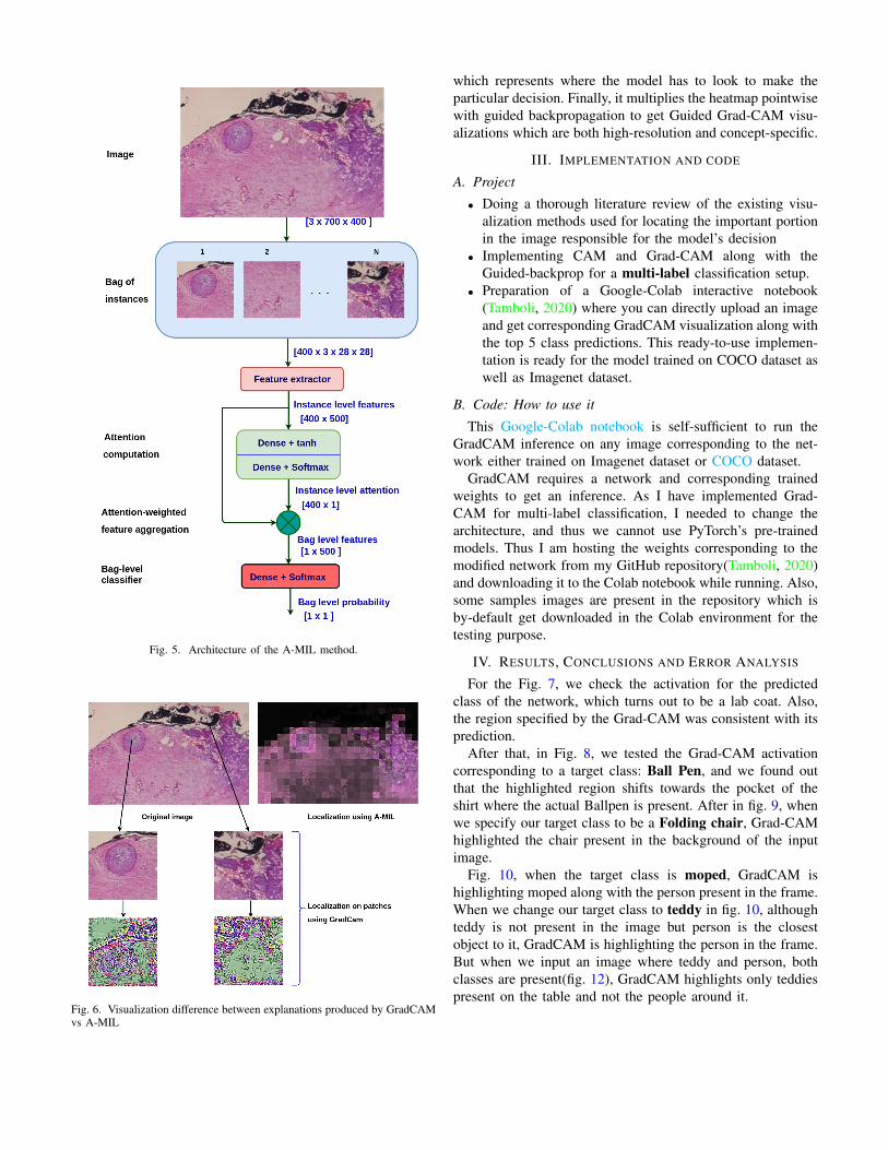
Fig. 5. Architecture of the A-MIL method.

Fig. 6. Visualization difference between explanations produced by GradCAMvs A-MIL

which represents where the model has to look to make theparticular decision. Finally, it multiplies the heatmap pointwisewith guided backpropagation to get Guided Grad-CAM visu-alizations which are both high-resolution and concept-specific.

III. IMPLEMENTATION AND CODE

A. Project

• Doing a thorough literature review of the existing visu-alization methods used for locating the important portionin the image responsible for the model’s decision

• Implementing CAM and Grad-CAM along with theGuided-backprop for a multi-label classification setup.

• Preparation of a Google-Colab interactive notebook(Tamboli, 2020) where you can directly upload an imageand get corresponding GradCAM visualization along withthe top 5 class predictions. This ready-to-use implemen-tation is ready for the model trained on COCO dataset aswell as Imagenet dataset.

B. Code: How to use it

This Google-Colab notebook is self-sufficient to run theGradCAM inference on any image corresponding to the net-work either trained on Imagenet dataset or COCO dataset.

GradCAM requires a network and corresponding trainedweights to get an inference. As I have implemented Grad-CAM for multi-label classification, I needed to change thearchitecture, and thus we cannot use PyTorch’s pre-trainedmodels. Thus I am hosting the weights corresponding to themodified network from my GitHub repository(Tamboli, 2020)and downloading it to the Colab notebook while running. Also,some samples images are present in the repository which isby-default get downloaded in the Colab environment for thetesting purpose.

IV. RESULTS, CONCLUSIONS AND ERROR ANALYSIS

For the Fig. 7, we check the activation for the predictedclass of the network, which turns out to be a lab coat. Also,the region specified by the Grad-CAM was consistent with itsprediction.

After that, in Fig. 8, we tested the Grad-CAM activationcorresponding to a target class: Ball Pen, and we found outthat the highlighted region shifts towards the pocket of theshirt where the actual Ballpen is present. After in fig. 9, whenwe specify our target class to be a Folding chair, Grad-CAMhighlighted the chair present in the background of the inputimage.

Fig. 10, when the target class is moped, GradCAM ishighlighting moped along with the person present in the frame.When we change our target class to teddy in fig. 10, althoughteddy is not present in the image but person is the closestobject to it, GradCAM is highlighting the person in the frame.But when we input an image where teddy and person, bothclasses are present(fig. 12), GradCAM highlights only teddiespresent on the table and not the people around it.

Fig. 7. Test image of myself, detected as Lab coat class

Fig. 8. Target class: Ball point pen, can see the focus shifted to the pocket from 7

Fig. 9. Target class: Folding Chair, the focus has shifted to the tiny chair in the background

Some critical observations:• Although GradCAM can detect the objects(pen, chair)

properly, but still, the probability for those classes arenot in the top5.

• As this is a multi-label classification setup, the sum ofprobabilities of all the classes does not sum up to theone, and thus multiple importance regions are visible.

• Fig. 11, GradCAM is highlighting the person for theclass teddy as it is the closest to the teddy class. Still,in fig. 12, both the teddy and person objects are present,GradCAM is properly locating only teddies present on thetable and not the people standing around it. This ensuresthat although the model thinks a person to be the nearestclass to the teddy, it is also able to discriminate betweenboth.

REFERENCES

S. Addepalli, D. Tamboli, R. V. Babu, and B. Banerjee.Saliency-driven class impressions for feature visualizationof deep neural networks. In 2020 IEEE International

Conference on Image Processing (ICIP), pages 1936–1940,2020. doi: 10.1109/ICIP40778.2020.9190826.

A. Patil, D. Tamboli, S. Meena, D. Anand, and A. Sethi.Breast cancer histopathology image classification and lo-calization using multiple instance learning. In 2019 IEEEInternational WIE Conference on Electrical and ComputerEngineering (WIECON-ECE), pages 1–4, 2019. doi: 10.1109/WIECON-ECE48653.2019.9019916.

Ramprasaath R Selvaraju, Michael Cogswell, Abhishek Das,Ramakrishna Vedantam, Devi Parikh, and Dhruv Batra.Grad-cam: Visual explanations from deep networks viagradient-based localization. In Proceedings of the IEEEInternational Conference on Computer Vision, pages 618–626, 2017.

Dipesh Tamboli. Interactive gradcam. https://github.com/Dipeshtamboli/Interactive-GradCAM, 2020.

Jason Yosinski, Jeff Clune, Anh Nguyen, Thomas Fuchs, andHod Lipson. Understanding neural networks through deepvisualization. arXiv preprint arXiv:1506.06579, 2015.

Bolei Zhou, Aditya Khosla, Agata Lapedriza, Aude Oliva, andAntonio Torralba. Learning deep features for discriminative

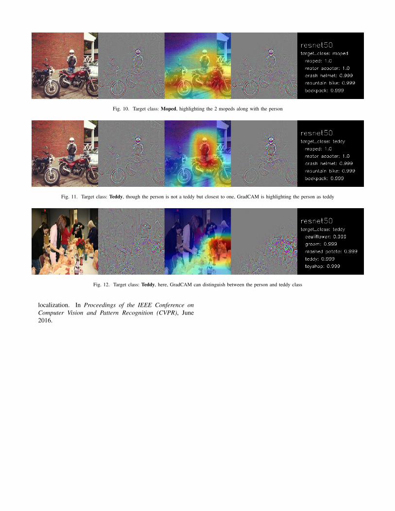
Fig. 10. Target class: Moped, highlighting the 2 mopeds along with the person

Fig. 11. Target class: Teddy, though the person is not a teddy but closest to one, GradCAM is highlighting the person as teddy

Fig. 12. Target class: Teddy, here, GradCAM can distinguish between the person and teddy class

localization. In Proceedings of the IEEE Conference onComputer Vision and Pattern Recognition (CVPR), June2016.