Munich Personal RePEc Archive

Explaining learning gaps in Namibia:

The role of language proficiency

Garrouste, Christelle

European Commission - Joint Research Centre (EC-JRC), UnitG.09Econometrics and Applied Statistics (EAS)

2011

Online at https://mpra.ub.uni-muenchen.de/25066/

MPRA Paper No. 25066, posted 24 Jun 2011 21:02 UTC

1

Explaining learning gaps in Namibia: the role of language proficiency

Christelle Garrouste*

Abstract

In a multilingual context, this study investigates the role of language skills on mathematics achievement. It compares characteristics of 5048 Grade-6 learners in 275 Namibian schools. The outcome variable is the standardized SACMEQ mathematics score collected in year 2000. Hierarchical linear modeling is used to partition the total variance in mathematics achievement into its within- and between-school components. The results do confirm the positive correlation between strong language skills variations at the school-level and low pupil mathematics scores, which may question the capacity of the current bilingual policy to provide for an effective and equal learning environment.

Keywords: Learning achievement; language skills; multilevel analysis; HLM JEL classification: C13, C3, I2.

∗ Christelle Garrouste, PhD. European Commission - Joint Research Centre (EC - JRC), Institute for the protection and Security of the Citizen (IPSC), Unit G.09 Econometrics and Applied Statistics (EAS). Email: christelle.garrouste@jrc.ec.europa.eu

Acknowledgements: The author would like to acknowledge SACMEQ for providing the Data Archive used in this study. Earlier versions of this paper have been improved by thoughtful comments and suggestions from anonymous peer reviewers and colleagues at the IIE (Stockholm University), at the Department of Economics of Padua University and at the JRC-IPSC-EAS (European Commission, Ispra), especially Paola Annoni. This work is part of a broader research project financed by a PhD position from Stockholm University (2002-2006). The usual disclaimer applies.

2

1.1 Introduction

The need for reconstruction after the Second World War has rapidly led to a world-wide

growth of interest in the application of large-scale scientific survey research techniques to

the study of issues related to improving the productivity of workers through an increase of

the number of literate people, among which Husén’s (1969) work and the international

research ran by the Association for the Evaluation of Education and Achievement (IEA) in

the early 1970s which encompassed twenty-three countries (see Elley, 1992, 1994;

Lundberg & Linnakyla, 1993; Postlethwaite & Ross, 1992). This trend spread

progressively to developing countries. In the 1980s the focus of these surveys slowly

moved from an increase of quantity of education to an improvement of quality of

education. Most occidental countries and an increasing number of developing countries are

now applying such techniques to undertake systematic studies of the conditions of

schooling and student achievement levels.

Summarizing the results of the IEA and other studies for developing countries,

Alexander & Simmons (1975) note the lack of consistency across studies and the

conflicting nature of the results. For instance, school-related variables, such as class size,

school size, and teacher characteristics, appeared to be significant in some countries and

non-significant (or negatively significant) in others. Finally, although non-school variables

appeared of high importance in all the studies, home background seemed to have less

influence on pupils’ performance in developing than in developed countries.

In the early 1980s, Heyman & Loxley (1983a; 1983b) examined the effects of

socioeconomic status and school factors on students’ science achievement in primary

school in sixteen low-income countries and thirteen high-income countries. They observed

that the influence of family background varied significantly with national economic

development between countries, and that the percentage of achievement variance explained

3

by school and teacher variables was negatively correlated with the level of a country’s

development. This result was confirmed by Saha (1983) and Fuller (1987) who examined

the effects of school factors on student achievement in the Third World. Fuller concluded

that “much of this empirical work suggests that the school institution exerts a greater

influence on achievement within developing countries compared to industrialized nations,

after accounting for the effect of pupil background” (pp. 255-6; italics in original).

Yet, more recent works based upon more sophisticated survey data have questioned

the sustainability of these results (see Gameron & Long, 2007, for a detailed discussion of

the evolution of the debate on equality of educational opportunity in the past four decades).

For instance, Baker, Goesling and Letendre (2002), who examined data from the Third

International Mathematics and Science Study (TIMSS) of 1995 and 1999, concluded that

Heyneman & Loxley’s findings for the 1970s were not observable anymore two decades

later. Baker et al. (2002) attributed the “Heyneman-Loxley effect” to the lack of mass

schooling investments in most developing countries back in the 1970s. They argued that

the expansion of education systems in developing countries during the 1980s and 1990s

was likely to have generated better educated cohorts of parents. Thus, developing countries

had beneficiated from a catching-up effect towards developed countries’ relative

composition of family and school effects on student outcomes. The authors conjectured,

however, that the Heyneman-Loxley effect might persist in countries where extreme

poverty or social upheaval such as civil war or epidemics slowed down mass schooling.

Chudgar & Luschei (2009) also revisited the Heyneman-Loxley hypothesis, using

the 2003 TIMSS data from 25 countries. They found that in most cases, family background

was more important than schools in understanding variations in student performance, but

that, nonetheless, schools were a significant source of variation in student performance,

especially in poor and unequal countries.

4

Focusing exclusively on Southern and Eastern African countries, the survey by the

Southern and Eastern Africa Consortium for Monitoring Educational Quality (SACMEQ)

revealed corroborative results. In 2005, the SACMEQ II1 national reports showed that most

countries were demonstrating large between- and within-school variations. While within-

school variation is an indication of differences in abilities among learners within each

school, between-school variations are an indication of equity problems within the

education system. South Africa, followed by Uganda and Namibia, demonstrated then the

highest percentage of between-school variation (see, for instance, Gustafsson, 2007, for a

detailed analysis of the South African case).

More specifically, the Namibian results displayed very poor learners and teachers

reading and mathematics scores, a definite decline in reading scores between the first

SACMEQ study of 1995 and the second one of 2000 and considerable variation among

regions (Makuwa, 2005). These results deserve further investigation in view of the high

resource allocation efforts made by the Namibian authorities to launch substantial

education reforms since independence in 1990, which included the adoption of a bilingual

language-in-education policy aiming primarily at facilitating the cognitive development

and, hence, the learning process of pupils (Skutnabb-Kangas & Garcia, 1995).

Hence, after a short review of the status of Namibian schools and political agenda

at the time the SACMEQ II was conducted (i.e. year 2000) (section 1.2), this paper

attempts to investigate the main factors explaining the poor scores of Namibian Grade-6

learners. More specifically, the objective is to see whether the home language and

1 The International Institute for Educational Planning (IIEP) designed the Southern Africa Consortium for Monitoring Educational Quality (SACMEQ) in 1991-1993, together with a number of Ministries of Education in the Southern Africa Sub-region. In 1995 the first SACMEQ survey project was launched in six Southern African countries. The SACMEQ I project was completed in 1998 followed by the SACMEQ II project launched in 2000 in fourteen Southern and Eastern African countries.

5

proficiency in English constitute significant discrimination factors in mathematics

achievement to explain the within-school and between-school variations.

This focus is geared by findings from other studies that have highlighted the

significant role of language proficiency on academic achievement. For instance, Geary,

Bew-Thomas, Liu & Stigler (1996) found that the language structure of Asian numbering

assisted Chinese children in developing meaningful early number concepts. Valverde

(1984) noted that differences in the English and Spanish languages contributed to Hispanic

Americans’ poor performance and involvement in mathematics (see also Bush, 2002, for

similar conclusions). Howie (2002, 2005) applied multilevel analysis (2002, 2005) on

South African TIMSS data to show that significant predictors of between-school variations

include pupils’ performance in the English test, their exposure to English and the extent to

which English is used in the classroom.

The method used in our work is a specific type of multilevel analysis called

Hierarchical Linear Modeling (HLM). This paper follows the theoretical steps enounced by

Bryk & Raudenbush (1988) and Hox (1995) for the use of the HLM method for education

analyses (see section 1.3 for a description of the model and data). The results are then

presented in section 1.4 and conclusions drawn in section 1.5.

1.2 Namibia’s School Structure and Policy Agenda at the Time of the Study

The Republic of Namibia is situated on the south west coast of Africa and is bordered by

the Atlantic Ocean to the west, the republics of Angola and Zambia to the north and north-

east respectively and the republics of Botswana and South Africa to the east and south

respectively. It obtained national independence from former apartheid South African

government on March 21, 1990, after many years of political, diplomatic and armed,

national liberation struggle. Even if the country is well endowed with good deposits of

6

uranium, diamonds, and other minerals as well as rich fishing grounds, there are wide

disparities in the distribution of incomes. With a per capita income of US$2,000 Namibia

may be regarded as a middle income country. Yet, the richest 10 percent of the society still

receives 65 percent of the incomes. As a consequence, the ratio of per capita income

between the top 5 percent and the bottom 50 percent is about 50:1 (Makuwa, 2005). This

provides a brief understanding of the socio-economic context under which the education

system has to develop in Namibia.

Since independence, Namibia has made strides in the provision of basic education,

which by 2001 had resulted in a primary education net enrolment of 94 percent of all

children aged 7-13 (in Grades 1-7), and by 2006 Namibia ranked among the top eight

African countries in term of primary completion rate (>80 percent) (Vespoor, 2006). While

much seems to have been achieved in terms of access to schooling, the quality of

education, efficiency and equity issues are since the late 1990s at the center of political

preoccupations.

Because Article 20 of the Constitution of the Republic of Namibia provides for free

and compulsory education for all learners between the ages of 6 and 16 or learners from

Grade 1 up to the end of Grade 7; and because the government has declared education to

be a priority among all other priorities in Namibia, education has received the largest share

of the national recurrent budget since independence. For instance, out of the estimated total

government current expenditure of N$8.35 billion for the 2001/2002 financial year, N$1.86

billion, i.e. about 20 percent of the budget, was earn-marked for basic education only. Of

the total amount allocated for basic education, N$986.56 million was earn-marked for

primary education and the rest for secondary education. Yet, almost 90 percent of the

money allocated for primary education was spent on personnel costs (e.g., salaries and/or

subsidies to teachers in a number of private schools), leaving only about 10 percent for all

7

the other services and school supplies (Makuwa, 2005). As a consequence, the financial

allocation per learner ratio is more favorable to regions with more qualified staff and fewer

learners than to rural regions with more unqualified teachers and large pupil-teacher ratios.

Finally, the fact that schools are authorized to collect school development funds directly

from parents is again more favorable to schools located in urban areas where parents have

an income than to schools in more remote areas.

In addition to these resource allocation issues, it is also important to highlight the

many changes that took place in the education sector between 1995 and 2000. As

explained in Makuwa’s (2005) report, there were for instance more learners and more

schools in 2000 than in 1995; the department of Sport was added to the Ministry of Basic

Education and Culture; and, more important, the HIV/AIDS pandemic became a national

problem affecting infected administrators, teachers, learners and/or parents. In view of

these new contextual settings, the Ministry of Basic Education, sports and Culture

(MBESC) defined eight new national priority areas in its “Strategic Plan” for the period

2001-2006: equitable access; education quality; teacher education and support; physical

facilities; efficiency and effectiveness; HIV/AIDS; lifelong learning; and sports, arts and

cultural heritage.

Finally, to understand the context framing the data used in this study, it is also

essential to give an overview of the structure of the Namibian primary school system. The

primary phase consists of the Lower Primary (Grades 1-4), during which mother tongue is

used as medium of instruction, and Upper Primary (Grades 5-7), during which English

becomes the medium of instruction up to Grade 12. By the year 2000, there were 998

primary schools hosting a total of 406,623 learners, of which 952 were government schools

and the rest were private schools. Nearly two thirds of all primary schools were located in

8

the six most populated northern regions namely, Caprivi, Kavango, Ohangwena, Oshikoto,

Oshana and Omusati.

It is in the above milieu that the second SACMEQ survey used in the present paper

was collected and it is therefore in that frame that the results of the analysis should be

interpreted.

1.3 Model and Data

The methodological approach applied in this study is a hierarchical linear modeling. The

HLM framework was developed during the 1980s by Aitkin & Longford (1986), DeLeeuw

& Kreft (1986), Goldstein (1987), Mason et al. (1983) and Raudenbusk & Bryk (1986). As

explained by Raudenbush & Bryk (1995), these procedures share two core features. First,

they enable researchers to formulate and test explicit statistical models for processes

occurring within and between educational units, thereby resolving the problem of

aggregation bias under appropriate assumptions. Second, these methods enable

specification of appropriate error structures, including random intercepts and random

coefficients, which can solve the problem of misestimated precision that characterized

previous conventional linear models and hindered their capacity to test hypotheses. Hence,

Lynch, Sabol, Planty & Shelly (2002) confirm the strength of HLM models compared to

other multilevel models to produce superior unbiased estimates of coefficients and robust

standard errors even when the assumptions required by OLS are violated.

The theoretical framework of HLM modeling we apply is the one derived from

Bryk & Raudenbush (1988) and defined by Hox (1995) consisting in 5 steps: (1) the Null

Model; (2) the estimation of the fixed effects of the within-school model; (3) the estimation

of the variance components of the within-school model; (4) the exploration of between-

9

school effects; and (5) the estimation of the cross-level interactions between the within-

and between-school variables.

Hence, the first step in fitting an HLM model is to analyze a model with no

explanatory variables, namely the Null Model. This intercept-only model is defined by:

⎪⎩

⎪⎨⎧

+=

+=

jj

ijjij

U

Ry

0000

0

μβ

β (1)

Hence,

ijjij RUy ++= 000μ . (2)

In this null model, ijy is the total raw mathematics score of individual i in school j and the

base coefficient j0β is defined as the mean mathematics score in school j. Whereas ijR

represents the pupil-level effect with variance )var( ijR (within-school variance), i.e. the

variability in student mathematics scores around their respective school means, jU0

represents the random school-level effect with variance 0000 )var()var( τβ =≡ jjU

(between-school variance), i.e. the variability among school means. For simplicity, we

assume ijR to be normally distributed with homogeneous variance across schools, i.e.

).,0(~ 2σNRij Hence, this intercept-only model is a standard one-way random effects

ANOVA model where schools are a random factor with varying numbers of students in

each school sample (Bryk & Raudenbush, 1988, p.75).

10

From the estimation of the within- and between-school variances, it is possible to

derive the intra-school correlation ρ, which is the ratio of the between-school variance over

the sum of the between- and within-school variances, to measure the percentage of the

variance in mathematics scores that occurs between schools. This first result serves at

justifying the conduct of further variance analyses at the within-school and between-school

levels when introducing pupil-level and school-level explanatory factors.

If the intra-school correlation ρ derived from equation (2) proves to be more than

trivial (i.e., greater than 10% of the total variance in the outcome) (Lee, 2000), the next

phase consists in analyzing a model with pupil-level (within-school) explanatory variables

ijX fixed. This implies that the corresponding variance components of the slopes are fixed

to zero. See Table 1 for a definition and statistics summary of the ijX parameters. This

fixed within-school model yields:

ijjpijp

ijijjjij

RUX

RXy

+++=

++=

0000

10

μμ

ββ , (3)

where the number of within-school explanatory variables ijX is p = 1,…,n; 00μ is the

average score for the population of each school group; 0pμ is the slope of the average ratio

between each within-school variable and the pupil’s mathematics score in each type of

school; and jU 0 is the unique effect of school j on mean mathematics score holding ijX

constant. For each school j, effectiveness and equity are described by the pair ),( 10 jj ββ

(Raudenbush & Bryk, 2002).

The third step consists now in assessing whether the slope of any of the explanatory

variables has a significant variance component between schools. The model considered is:

11

ijjpijpjpijpij RUXUXy ++++= 0000 μμ, (4)

where pjU is the unique effect of school j on the slope of the ratio between each within-

school variable ijX

and the pupil’s mathematics score holding ijX constant. We assume

jU 0 and pjU to be random variables with zero means, variances 00τ

and 11τ respectively,

and covariance 01τ .

The testing of random slopes variations is done on a one-by-one basis. As explained

by Raudenbush & Bryk (1987; 1988; 1992; 1995), the unconditional model is particularly

valuable because it provides estimates of the total parameter variances and covariances

among the βpj. When expressed as correlations they describe the general structure among

these within-school effects. Moreover, HLM derives an indicator of the reliability of the

random effects by comparing the estimated parameter variance in each regression

coefficient, var(βij), to the total variance in the ordinary least square estimates.

Next, the higher level explanatory variables qjZ (i.e., school-level factors, see

Table 1) are added to equation (4) to examine whether these variables explain between-

school variations in the dependent variable. This addition yields:

ijjpijpjqjqpijpij RUXUZXy +++++= 00000 μμμ , (5)

with q between-school explanatory variables Z, q = 1,…,m.

The between-school variables add information about the quality of teaching and the

learning environment. The FML estimation method is again used to test (with the global

chi-square test) the improvement of fit of the new model.

12

Finally, cross-level interactions between explanatory school-level variables and

those pupil-level explanatory variables that had significant slopes variation in equation (4)

are added. This last addition leads to the full model formulated in equation (6):

ijOjpijpjpijqjpqqjqpijpij RUXUXZZXy ++++++= μμμμ 0000 , (6)

Here again, the FML estimation method is used to derive the global chi-square test to

assess the improvement of fit.

Note that relevance to the Namibian context, correlations with test scores and

correlations between input variables were taken into account in the selection of all the

within-school pijX

and between-school qjZ parameters retained for this model (see Table

1 for a description of all variables). The data used to test this model are taken from the

SACMEQ II survey. The sampling procedure for that survey was geared by

methodological recommendations to all participating countries, but with certain flexibility

to take into account contextual differences. Hence, as for all other participating countries,

the desired target population in Namibia was all learners enrolled in Grade 6 in the ninth

month of the school year (i.e. in September 2000). The net enrolment ratio for the age

group 7-13 years old who were enrolled in Grades 1 to 7 in Namibia in 2000 was 91.3

percent. However, in Namibia it was decided to exclude certain learners namely, learners

in schools with less than fifteen Grade 6 learners, learners in “inaccessible” schools, and

learners in special schools. A two-stage cluster sampling was applied using approximately

equal size clusters stratified into the 13 educational regions, which led to a final sample of

5048 learners and 275 schools (Makuwa, 2005)1. The SACMEQ II Mathematics and

Reading tests were conducted in English.

13

The HLM6.0 program was used in this study to partition the total variance in

mathematics scores into its within- and between-school components according to the

methodological steps described above.

1.4 Results

As explained in the previous section, the output variable of our HLM model is pupil’s total

raw score in mathematics at the SACMEQ test (MATOTP). The SACMEQ II Mathematics

test is composed of three domains, namely (1) number (i.e. operations and number line,

square roots, rounding and place value, significant figures, fractions, percentages, and

rations); (2) measurement (i.e. measurements related to distance, length, area, capacity,

money, and time); and (3) space-data (i.e. geometric shapes, charts and data tables)2.

1.4.1 The Null Model

From equations (1) and (2) we find that the within-school variance )var( ijR , i.e. the

variability in student mathematics scores around their respective school means, is

estimated to 25.56 and the between-school variance )var()var( 00 jjU β≡ , i.e. the

variability among school means, is estimated to 36.02. Consequently, the intra-school

correlation ρ, i.e. the ratio of the between-school variance over the sum of the between-

and within-school variances, is .585, which implies that approximately 58.5 percent of the

variance in mathematics scores occurs between schools. This result confirms the

proportion of between-school variations estimated by Makuwa (2005) in Namibian

mathematics and reading scores, namely approximately 60 percent between-school

variation against 40 percent within-school variation.

The Full Maximum Likelihood (FML) estimation method was used to calculate the

value of deviance of this intercept-only model, which is a measure of the degree of misfit

14

of the model (McCullagh & Nelder, 1989; Hox, 1995). In the HLM6.0 software estimates

the deviance as Ldeviance log2−= (Peugh, 2010). From the FML estimation of our null

model we obtained a deviance of 31575.86 (with 3 estimated parameters). Hence, each of

the following steps of this HLM analysis aimed at fitting a model with a lower deviance

value and the highest explanatory capacity.

1.4.2 The Within-School Model: Fixed-Effect Unconditional Model

The next phase consisted in analyzing a model with pupil-level (within-school)

explanatory variables fixed. This implies that the corresponding variance components of

the slopes were fixed to zero (see equation (3)). Based upon relevance to the Namibian

context, correlations with test scores and correlations between input variables3, five pupil-

level explanatory variables (i.e. six parameters when including the intercept namely, the

base score) were retained: ENGLISH, FEMALE, SES, RATOTP and REPEAT. Table 1

defines each of these variables and presents their summary statistics.

The variable ENGLISH explores the role played by the practice of English at home

in learning achievement in a country that applies a bilingual education policy based on

mother-tongue instruction in the early phase of primary education before transiting to

English in Grade 5 upwards. It is nevertheless important to highlight that because of the

nature of the question – “How often do you speak English at home?” – inconsistency in the

responses is plausible. For instance, the fact that 76.9 percent of the sampled pupils

answered that they speak sometimes or all the time English at home does not mean that

English is the mother-tongue of 76.9 percent of that population. In reality, English is the

mother-tongue of only .56 percent of the Namibian population (Gordon, 2005). Moreover,

no indication is provided about the nature and the level of communication in English that is

15

occurring at home. Hence, this home language parameter should not be interpreted as a

proxy of mother-tongue rather as a proxy of the linguistic home background of the pupil.

Further, with regard to the gender variable, FEMALE, in the present case, although

the mean mathematics score for boys (= 18.86) is very close to the one for girls (= 18.25)

the existence of very high variance within each group (66.41 for boys and 56.45 for girls)

justifies further exploration. In turn, SES is a computed variable measuring the pupil’s

socio-economic status (in terms of parents’ education, possessions at home, light, wall,

roof, floor) that takes values between 1 and 15. RATOTP is the pupil’s total raw score in

reading at the SACMEQ test. The reading test scores serve here as a proxy of English

language proficiency (see Geary et al., 1997; Valverde, 1984; Collier, 1992; Ehindero,

1980; Yip et al., 2003; Clarkson & Galbraith, 1992). Note that the strong correlation

expected between RATOTP and ENGLISH is present in our sample with a significance at

the .01 level (2-tailed) and that the mean reading score of pupils who never speak English

at home (= 29.86) is less than the mean score of pupils speaking sometimes or all the time

English at home (= 35.00).

Finally, REPEAT is a dummy variable taking the value of 1 if the pupil has

repeated at least one class and 0 if not. It provides information on the learning

facilities/difficulties of the pupil and serves thereby as a proxy of the pupil’s academic

background when combined with RATOTP (Bryk & Raudenbush, 1988). In our sample the

mean mathematics score of grade repeating pupils is 16.66 compared to 20.55 for pupils

on-track with much larger variance among the first (= 87.95) than among the latter group

(= 29.18).

Replacing each parameter by its label-value in equation (3) we get:

16

ijjijjij

jijijijij

RUREPEATRATOTPRATOTP

SESSESFEMALEENGLISHMATOTP

+++−+

−+++=

•

•

05040

30201000

)(

)(

μμ

μμμμ , (3’)

where the predictors SES and RATOTP are centered around their respective group mean.

The final estimation of these fixed effects with robust standard errors is displayed

in Table 2. It appears that the most significant parameters are the average mathematic

scores at the school-level ( 0μ ), the pupil’s gender ( 2μ ) and the pupil’s English proficiency

level ( 4μ ) (adjusted for the average English proficiency in the school). The slope signs

show that, whereas being a girl has an overall negative impact on individual mathematics

scores, a high mean mathematics score in the school and an individual English proficiency

above the school average have a positive impact on individual mathematics scores.

Note that the lack of statistical significance of the ENGLISH, SES and REPEAT

parameters is not strong enough to justify at this stage a removal from the model. Rather,

what the model shows so far is that speaking English at home and a higher SES

background than the school average have a positive impact (i.e. positive correlation sign)

on mathematics achievement, which confirms the theory. Moreover, grade repetition is

negatively correlated with mathematics achievement, which confirms the conclusions

reached by Verspoor (2006) in his report for ADEA. Yet, before claiming that this result

either invalidates or confirms the assumption that repetition has a negative effect on pupil’s

achievement ‘improvement’, it is important to highlight that the SACMEQ dataset does not

provide for any longitudinal data. This lack implies that it is impossible to know whether

the pupil who repeated a grade did improve its mathematics score compared to the

previous year or not. All we know from the present analysis is that, overall, pupils who

have repeated a grade perform less well than their non-repeating peers. Hence, combined

with RATOTP, the REPEAT variable gives us an idea of the role of the educational

17

background of the pupil on mathematics scores at a fixed date t, with a higher mathematics

achievement when the pupil is on school track (no repetition) and highly proficient in

English.

The deviance of this model is 30002.99 (number of estimated parameters = 8)

which means an improvement from the null model. This fixed unconditioned model

explains 61.7 percent of the total variance in mathematics scores. The explanatory power

of this unconditioned fixed effect model will be compared to the explanatory power of the

final full model to assess the improvement of fit obtained through this hierarchical linear

modeling process (see Table 4).

1.4.3 The Within-School Model: Random-Effect Unconditional Model

The third step consisted in assessing whether the slope of any of the explanatory variables

has a significant variance component between schools:

ijjijjj

ijjjijjijj

ijjijjij

jijijijij

RUREPEATURATOTP

RATOTPUSESSESUFEMALEU

ENGLISHUREPEATRATOTPRATOTP

SESSESFEMALEENGLISHMATOTP

+++−

+−++

++−+

−+++=

•

•

•

•

05

432

15040

30201000

)

()(

)(

)(

μμ

μμμμ

, (4’)

where the predictors SES and RATOTP are centered around their respective group mean.

The testing of random slopes variations was done on a one-by-one basis. Table 2

presents all the results for the within-school explanatory models (with fixed-effects and

with random-effects). At this first level of the HLM, the models are still unconditioned by

the between-school variables. As explained by Raudenbush & Bryk (1987; 1988; 1992;

1995), the unconditional models are particularly valuable because they provide estimates

18

of the total parameter variances and covariances among the βpj. When expressed as

correlations they describe the general structure among the within-school effects.

Table 2 shows that a high base level of achievement is associated with less grade

repetition (r = .974), higher English proficiency (r = .915), higher SES (r = .602), and male

pupils (r = .650) who do not have English as home language (r = .192). There is also a

substantial association between pupil high SES and academic achievement (with a high

negative correlation between SES and grade repetition (r = .624) and a positive correlation

with English proficiency (r = .278)).

Moreover, HLM derives an indicator of the reliability of the random effects by

comparing the estimated parameter variance in each regression coefficient, βij, to the total

variance in the ordinary least square estimates. These results are also displayed in Table 2.

As expected, the base score is rather reliable, .788, compared to the regression coefficients

which range from .036 for pupils’ SES to .315 for reading raw score (i.e. English

proficiency). This relatively low reliability may express the fact that much of the observed

variability among schools in regression slopes is due to sampling error that can not be

explained by within-school factors. The same test on the conditioned model will enable us

to ascertain or reject this interpretation.

Finally, the results of the homogeneity-of-variance tests provide statistical evidence

of significant variation within schools in each of the six random regression coefficients

(with high Chi-square statistics and 233 degrees of freedom). The probability of the

observed variability in these coefficients, under a homogeneity hypothesis, is less than .001

for β0 (base score coefficient) and β4 (English proficiency coefficient) and less than .20 for

β5 (repetition coefficient). This means that schools vary significantly in the degree to which

achievement in mathematics depends on the child’s reading score in English and repetition

status, i.e. on the child’s academic background, which confirms the findings by

19

Raudenbush & Bryk (1988). Despite low statistical significance, the pupil’s gender, SES

and home language status, are still retained as random parameters because of previously

reported school effects on each of them (see section 1.1).

1.4.4 The Between-School Model: Conditional Model

Next, the higher level explanatory variables qjZ (i.e., school-level factors) were added to

equation (4) to examine whether these variables explain between-school variations in the

dependent variable. This addition yields equation (5). The between-school variables add

information about the quality of teaching and the learning environment.

In this model, Zqj includes q=11 classroom and school parameters (see Table 1 for

details): TOTENROL which measures the size of the school in term of total enrolment;

PTRATIO providing the pupil-teacher ratio in each mathematics class; STYPE, a dummy

variable taking the value of 1 when the school is governmental and 0 when private; SLOC,

a dummy variable taking the value of 1 when the school is situated in an urban area and 0

when in a rural or isolated area; PRACAD, a measure of the proportion of pupils on track

(no grade repetition) in each school j; DISCLIM measuring the overall discipline climate of

the school; LGMNTY, a dummy variable taking the value of 1 when 40 percent or more of

the pupils speak English at home in school j and the value of 0 when less than 40 percent

never speak English at home (this computation follows Raudenbush & Bryk’s (1988)

computation of racial minority in the U.S. context); MSES, the mean SES in school j; TSEX

taking the value of 1 when the mathematics teacher is a female and the value of 0 when a

male; TSATPLRN taking the value of 1 when the mathematics teacher considers the pupils’

learning as very important and 0 when not important or of some importance; and

MATOTT, the mathematics raw score of the teacher, which serves as a proxy of the

teacher’s qualifications based on its mastery of the subject.

20

Replacing these variable labels into equation (5) yields:

ijjijj

jijjjijjijj

ijjjj

jjj

jjjj

jj

ijjij

jijijijij

RUREPEATU

RATOTPRATOTPUSESSESUFEMALEU

ENGLISHUMATOTTMATOTTTSATPLRN

TSEXMSESMSESLGMNTY

DISCLIMPRACADSLOCSTYPE

PTRATIOPTRATIOTOTENROLTOTENROL

REPEATRATOTPRATOTP

SESSESFEMALEENGLISHMATOTP

+++

−+−++

+−++

+−++

++++

−+−

++−+

−+++=

••

•

•

••

•

•

05

432

1011010

090807

06050403

0201

5040

30201000

)()(

)(

)(

)()(

)(

)(

μμ

μμμ

μμμμ

μμ

μμ

μμμμ

(5’)

where the predictors TOTENROL, PTRATIO, MSES, RATOTP and MATOTT are centered

around their respective grand mean.

The FML estimation method was again used to test (with the global chi-square test)

the improvement of fit of the new model. After adding the between-school explanatory

parameters, the deviance was reduced to 29495.19 with 39 degrees of freedom. Table 3

presents the results for this conditional model. What appears from this analysis is that the

proportion of students on track, the mean pupil’s SES and the level of mathematics of the

math teacher explain very significantly (significant at the .001 level) variations in the

individual mathematics scores. At a lesser level, the school’s overall disciplinary climate

and the type of school also play a significant role, with t-values of 1.812 and -1.281

respectively. The negative slope of the type of school indicates that private schools

perform on average better than governmental schools.

21

1.4.5 The Final Model: Cross-Level Interaction Model

Finally, cross-level interactions between explanatory school-level variables and the pupil-

level explanatory variables that had significant slope variations in equation (4) were added.

This last addition led to the full model formulated in equation (6) where the predictors SES,

RATOTP, TOTENROL, PTRATIO, MSES and MATOTT were centered around their

respective grand mean:

ijjijj

jijjjijjijj

ijjijjijj

ijjijj

jijj

jijjjijj

jijj

jijjijj

jijijj

ijijj

ijjijj

jjjjij

RUREPEATU

RATOTPRATOTPUSESSESUFEMALEU

ENGLISHUREPEATMSESMSESREPEATSTYPE

REPEATRATOTPRATOTPMATOTTMATOTT

RATOTPRATOTPMSESMSES

RATOTPRATOTPPRACADRATOTPRATOTPSTYPE

RATOTPRATOTPTOTENROLTOTENROL

RATOTPRATOTPSESSESDISCLIM

SESSESFEMALEMSESMSES

FEMALEENGLISHDISCLIM

ENGLISHSTYPEENGLISHMATOTTMATOTT

MSESMSESPRACADSLOCSTYPEMATOTP

+++

−+−++

+−++

+−−+

−−+

−+−+

−−+

−+−+

−+−+

++

++−+

−++++=

••

•

••

••

••

••

••

••

•

•

05

432

15251

5045

44

43142

41

4031

3021

2012

111005

0403020100

)()(

)(

))((

))((

)()(

))((

)()(

)()(

)(

)(

μμ

μμ

μ

μμ

μ

μμ

μμ

μμ

μμμ

μμμμμ

(6’)

Here again, the FML estimation method was used to derive the global chi-square test to

assess the improvement of fit. The deviance is now 29354.015 (with 44 estimated

parameters), which means a 7.57 percent improvement compared to the null model. The

OLS regression of the full explanatory model improved the capacity of explanation of the

variations in individual mathematics scores ( 2

FullR = 63.5 percent) by almost 2 percent

compared to the unconditioned model ( 2

nedUnconditioR = 61.7 percent).

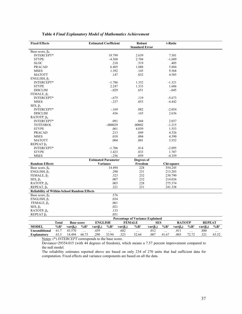
The results of the final explanatory model are displayed in Table 4 and show that

the base score differences between private and public schools (STYPE) disappear once the

22

school location (SLOC), the portion of pupils on track (PRACAD), the mean SES (MSES)

of the school and the mathematics score of the math teacher (MATOTT) are taken into

account. The negative slope of the school type means that greater mathematics

achievement is associated with private schools situated in urban areas, with a high

proportion of pupils on track, a high average SES and a good mastery of mathematics by

the teacher. The effect of the school type (public or private) on the attraction of home-

English speaking pupils disappears once the disciplinary climate (DISCLIM) is taken into

account. Home-English speaking pupils tend to attend private schools where the

disciplinary climate is safer. Furthermore, low average school SES tends to be more

associated with boys than with girls (FEMALE) and pupil’s SES is associated to important

disciplinary problems. Greater reading scores are associated with public schools if they are

of small size (TOTENROL), if the proportion of pupils on track is high and the school

average SES is not too low. In addition, great reading scores are also associated with a

good mastery of mathematics by the math teacher. Finally, there seems to be less grade

repetition in public schools and in schools with a lower average SES.

The most rigorous test of the explanation power of the final model of our HLM

analysis involves acceptance of the homogeneity of residual variance hypotheses, i.e. “after

modeling each βpj as a function of some school-level variables, is there evidence of

residual parameter variation in the βpj that remains unaccounted?” (Bryk & Raudenbush,

1988, p.79). Table 4 shows evidence of significant residual variation (high Chi-square) in

base achievement score and academic background (RATOTP and REPEAT) and the

homogeneity hypothesis for the home language (p > .500), gender (p > .500) and social

differentiation (p > .500) is still not sustained. This means that the remaining variance in

βpj might be due to sampling variance arising because pjβ̂ measures βpj with error (i.e.

23

pjpjpj R+= ββ̂ ) and because of the existence of correlation between Xpij and Upj (i.e.

0][ ≠pijpj XUE ) (see Pedhazur, 1982, for a comprehensive discussion of measurement

errors, specification errors, and multicollinearity and see our annex for a detailed

discussion on the significance of this potential endogeneity bias for the validity of our

results).

Finally, the last panel of Table 4 compares the residual parameter variances from

the explanatory model with the total parameter variances estimated in the unconditional

model (i.e. the difference between the estimated parameter variance in the null model and

the estimated parameter variance in the full model divided by the estimated parameter

variance in the null model; Roberts, 2007). The proportion reduction in these parameters’

variance can be interpreted as an indicator of the power of the explanatory model. The

fitted model accounts for a substantial percentage of the variance of each within-school

parameters ranging from 33.94 percent for the home language parameter (ENGLISH) to

72.72 percent for the individual reading scores (RATOTP) which constitutes our English

proficiency proxy.

1.5 Conclusions

In sum, our HLM analysis provides empirical support for the contention that academic

organization and normative environment of schools have a substantial impact on the social

distribution of achievement within them (58.5% of the variance in mathematics scores is

explained by the presence of heterogeneity between schools). On the one hand, at the

individual level, the base mathematics score of the school, followed by the academic

background of the pupil (RATOTP and REPEAT), its gender as well as its home language

play a statistically significant role in the individual mathematics achievement. On the other

24

hand, at the school level, the analysis shows that, overall, individual mathematics

achievement is facilitated in schools with a higher proportion of students on-track

(REPEAT), a higher average SES and a strong mastery of the subject by the mathematics

teacher (MATOTT). Pupils also tend to perform better in private schools than in

governmental schools (STYPE) which confirms the observed tendency for higher

achievement in schools with less disciplinary problems (DISCLIM).

With regard to language parameters, although the use of English at home looses a

bit of its statistical significance when comparing between-school variations, its coefficient

remains very high and confirms it as an important factor of variation in mathematics

scores. Moreover, the language proficiency parameter (RATOTP) increases even more its

explanatory capacity at the between-school level which makes it the most significant

explanatory variables of this model.

The policy and research implications of these results are four-fold. First of all, the

confirmed strong role played by linguistic parameters on learning achievement should

incite decision makers to focus their attention on assessing the effectiveness and equity of

the language-in-education policy (LiE) (Garrouste, 2007). From our analysis, it appears

that the individual low scores in Mathematics are strongly driven by overall low

achievement scores and strong within-school variations in English proficiency. This result

questions both the capacity of the Namibian bilingual policy to compensate for

heterogeneous individual exposure to the English language at home (equity) and its

efficiency to provide for a high instruction level in English by all schools (effectiveness).

The real source of this inefficiency should therefore be investigated further at the micro

level through a detailed questionnaire on the pupils’ and teachers’ home language to

estimate the proportion of pupils actually receiving their primary phase instruction in their

mother tongue. This information should then be complemented with a test-based

25

assessment of the literacy level in mother tongues to understand whether the low levels of

reading skills in English are indeed driven by low levels of mother tongue literacy.

Moreover, our study also reveals the need for an improvement of the quality of

resource allocations in teacher training as a prerequisite to improve the subject mastery of

teachers, but also in the development of better supervision structures to improve the

disciplinary climate in governmental schools. Thirdly, it appears important to investigate

the potential negative direct effect (on the targeted pupil) and indirect effect (via peer-

effect) of high repetition rates in primary education.

Finally, despite the fact that it is assumed to have a potential positive effect on the

fit of the final model in view of the HIV/AIDS pandemic affecting the whole country, the

health status of the pupils could not be accounted for by this study. Because less than half

of the pupils sampled (N=2199 out of 5048) answered the question related to the reasons of

their absenteeism (illness, work, family or fee not paid), and because of the very unspecific

nature of the question, this parameter could not be included in this analysis. In absence of

information about the type of illness or the duration of absenteeism in the SACMEQ II

dataset, the choice of this parameter as a proxy of the potential role of HIV/AIDS on

learning achievement would have been highly questionable.

Thus, based upon our analysis, we would like to recommend further efforts by all

concerned stakeholders to incorporate more appropriate linguistic data into large-scale

student/school surveys to better isolate the impact of LiE policies on the effectiveness and

equity of the Namibian schools.

Notes:

1 The parameters retained in this HLM analysis suffered no missing data, except for the

outcome variable. In the case of the total raw mathematics scores of the pupils, 58 cases

26

(1.1 percent) were missing because of non-completion of the test but these data could be

recomputed by estimating a probabilistic value from the school mean and the grand mean.

2 For a detailed overview of the levels and items composing the SACMEQ II Mathematics

test, see the blueprint in Makuwa (2005, p. 31).

3 Stem & Leaf plots of Mathematics scores by each parameter have been drawn and

revealed the existence of large variations between and/or within groups, which justify the

conduct of the present HLM analysis on these parameters to investigate the source of this

variance.

27

References

Aitkin, M., & Longford, N. (1986). Statistical Modeling Issues in School Effectiveness

Studies. Journal of the Royal Statistical Society, Series A, 149(1), 1-43.

Alexander, L., & Simmons, J. (1975). The Determinants of School Achievement in

Developing Countries: A Review of Research. Economic Development and Cultural

Change, 26, 341-58.

Baker, D.P., Goesling, B. & Letendre, G. (2002). Socio-Economic Status, School Quality

and National Economic Development: A cross-national analysis of the Heyneman-

Loxley effect. Comparative Education Review, 46: 291-313.

Billy, J.O.G. (2001). Better Ways to do Contextual Analysis: Lessons from Duncan and

Raudenbush. In A.C. Crouter (Ed.), Does it Take a Village?: Community Effects on

Children, Adolescents, and Families. Mahwah, NJ: Lawrence Erlbaum.

Bush, W.S. (2002). Culture and Mathematics: An Overview of the Literature with a View

to Rural Contexts. Working Paper Series, 2. Louisville: University of Louisville,

Appalachian Collaborative Center for Learning, Assessment and Instruction in

Mathematics.

Clarkson, P.C., & Galbraith, P. (1992). Bilingualism and Mathematics Learning: another

Perspective. Journal for Research in Mathematics Education, 23(1), 34-44.

Collier, V.P. (1992). A Synthesis of Studies Examining Long-Term Language Minority

Student Data on Academic Achievement. Bilingual Research Journal, 16(1&2), 187-

212.

DeLeeuw, J., & Kreft, I. (1986). Random Coefficient Models for Multilevel Analysis.

Journal of Educational Statistics, 11(1), 57-85.

28

Ehindero, O. J. (1980). The Influence of Two Languages of Instruction on Students’

Levels of Cognitive Development and Achievement in Science. Journal of Research

in Science Training, 17(4), 283-8.

Elley, W.B. (1992). How in the World do Children Read? The Hague: IEA.

Elley, W.B. (Ed.). (1994). The IEA Study of Reading Literacy: Achievement and

Instruction in Thirty-Two School Systems. Oxford: Pergamon Press.

Fielding, A., & Steele, F. (2007). “Handling Endogeneity by a Multivariate Response

Model: Methodological Challenges in Examining School and Area Effects on Student

Attainment”. Paper presented at the Sixth International Conference on Multilevel

Analysis, Amsterdam, April 16-17, 2007.

Frank, R. (2005). “Help or Hindrance?: A Multi-level Analysis of the Role of Families and

Communities in Growing up American”. Paper presented at the Population

Association of America’s Annual Meeting, Philadelphia, PA, March 31-April 3, 2005.

Fuller, B. (1987). What School Factors Raise Achievement in the Third World? Review of

Educational Research, 57(3), 255-97.

Gameron, A., & Long, D.A. (2007). Equality of Educational Opportunity: A 40-year

retrospective. In R. Teese, S. Lamb & M. Duru-Bellat (eds.), International Studies in

Educational Inequalty, Theory and Policy, Vol.1, Educational Inequality, Persistence

and Change. Dordrecht: Springer.

Garrouste, C. (2007). Determinants and Consequences of Language-in-Education Policies:

Essays in Economics of Education. Stockholm: Institute of International Education,

Studies in International and Comparative Education, 74.

Geary, D.C., Bow-Thomas, C.C., Liu, F., & Stigler, R.S. (1996). Development of

Arithmetic Computation in Chinese and American Children: Influence of Age,

Language, and Schooling. Child Development, 67, 2022-2044.

29

Goldstein, H. (1987). Multilevel Models in Educational and Social Research. Oxford:

Oxford University Press.

Gordon, R. G., Jr. (Ed.). (2005). Ethnologue: Languages of the World, 15th ed. Dallas,

T.X.: SIL International. URL: http://www.ethnologue.com/.

Grilli, L., & Rampichini, C. (2007). “Endogeneity Issues in Multilevel Linear Models”.

Paper presented at the Sixth International Conference on Multilevel Analysis,

Amsterdam, April 16-17, 2007.

Gustafsson, M. (2007). Using the Hierarchical Linear Model to Understand School

Production in South Africa. South African Journal of Economics, 75(1), 84-98.

Heyneman, S., & Loxley, W. (1983a). The Distribution of Primary School Quality within

High and Low Income Countries. Comparative Education Review, 27(1), 108-18.

Heyneman, S., & Loxley, W. (1983b). The Effect of Primary School Quality on Academic

Achievement across 29 high- and low-income countries. American Journal of

Sociology, 88(6), 1162-94.

Howie, S. (2002). English Language Proficiency and Contextual Factors Influencing

Mathematics Achievement of Secondary Schools in South Africa. Twente: University

of Twente, Unpublished PhD thesis.

Howie, S. (2005). System-Level Evaluation: Language and Other Background Factors

Affecting Mathematics Achievement. Prospects, XXXV(2), 175-186.

Hox, J.J. (1995). Applied Multilevel Analysis. Amsterdam: TT-Publikaties.

Husén, T. (1969). Talent, Opportunity and Career: A 26 Year Follow-up of 1500

Individuals. Stockholm: Almqvist & Wiksell.

Lamb, S., & Fullarton, S. (2002). Classroom and School Factors Affecting Mathematics

Achievement: A Comparative Study of Australia and the United States using TIMSS.

Australian Journal of Education, 46(2), 154-173.

30

Lee, V.E. (2000). Using Hierarchical Modeling to Study Social Contexts: The case of

school effects. Educational Psychologist, 35(2), 125-141.

Lundberg, I., & Linnakyla, P. (1993). Teaching Reading Around the World. The Hague:

IEA.

Lynch, J.P., Sabol, W.J., Planty, M., & Shelly, M. (2002). Crime, Coercision and

Community: the Effects of Arrest and Incarceration Policies on Informal Social

Control in Neighborhoods. Rockville, MD: National Criminal Justice Reference

Services (NCJRS).

Makuwa, D. (2005). The SACMEQ II project in Namibia: a Study of the Conditions of

Schooling and the Quality of Education. Harare: SACMEQ Educational Policy

Research Series.

Mason, W.M. (2001). Multilevel Methods of Statistical Analysis. On-Line Working Paper

Series, CCPR-006-01. Los Angeles, CA: University of California, California Center

for Population Research.

Mason, W.M., Wong, G.Y., & Entwistle, B. (1983). Contextual Analysis through the

Multilevel Linear Model. In S. Leinhardt (Ed.), Sociological Methodology 1983-1984,

14. San Francisco, C.A.: Jossey-Bass.

McCullagh, P., & Nelder, J.A. (1989). Generalized Linear Models. London: Chapman &

Hall.

Miller, J. E., & Phillips, J. A. (2002). Does Context Affect SCHIP Disenrollment?

Findings from a Multilevel Analysis. Working paper, 316. Chicago: Northwestern

University/University of Chicago Joint Center for Poverty Research.

Pedhazur, E.J. (1982). Multiple Regression in Behavioral Research: Explanation and

Prediction, 2nd ed. New York, NY: Holt, Rinehart and Winston.

31

Peng, X. (2007). Estimates of School Productivity and Implications for Policy. Columbia,

MO: University of Missouri-Columbia. Unpublished M.A. thesis.

Peugh, J.L. (2010). A practical guide to multilevel modeling. Journal of School

Psychology, 48, 85–112.

Postlethwaite, T., & Ross, K. (1992). Effective Schools in Reading: Implications for

Planners. The Hague: IEA.

Raudenbush, S.W., & Bryk, A.S. (1986). A Hierarchical Model for Studying School

Effects. Sociology of Education, 59(1), 1-17.

Raudenbush, S.W., & Bryk, A.S. (1987). Application of Hierarchical Linear Models to

Assessing Change. Psychological Bulletin, 101(1), 147-58.

Raudenbush, S.W., & Bryk, A.S. (1988). Toward a More Appropriate Conceptualization of

Research on School Effects: A Three-Level Linear Model. The American Journal of

Education, 97(1), 65-108.

Raudenbush, S.W., & Bryk, A.S. (1992). Hierarchical Linear Models: Applications and

Data Analysis Methods. Beverly Hills, C.A.: Sage Publications.

Raudenbush, S.W., & Bryk, A.S. (1995). Hierarchical Linear Models. In T. Husén & T.N.

Postlethwaite (Eds.), The International Encyclopedia of Education, 2nd ed., 5, 2590-6.

Raudenbush, S.W., & Bryk, A.S. (2002). Hierarchical Linear Models: Applications and

Data Analysis Methods. 2nd Edition. London: Sage Publications.

Rettore, E., & Martini, A. (2001). “Constructing League Tables of Service Providers when

the Performance of the Provider is Correlated to the Characteristics of the Clients”.

Paper presented at the Convegno Intermedio della Società Italiana di Statistica

Processi Metodi Statistici di Valutazione, Rome, June 4-6, 2001.

Roberts, J.K. (2007). Group Dependency in the Presence of Small Intraclass Correlation

Coefficients: An Argument in Favor of Not Interpreting the ICC. Paper presented at

32

the annual meeting of the American Educational Research Association, April 10,

2007.

Saha, L.J. (1983). Social Structures and Teacher Effects on Academic Achievement: A

comparative Analysis. Comparative Education Review, 27(1), 69-88.

Skutnabb-Kangas, T., & Garcia, O. (1995). Multilingualism for All – General Principles?

In Skutnabb-Kangas, T. (ed.), Multilingualism for All. Lisse: Swets & Zeitlinger B.V.,

European Studies on Multilingualism, 4, 221-256.

Valverde, L.A. (1984). Underachievement and Underrepresentation of Hispanics in

Mathematics and Mathematics Related Careers. Journal for Research in Mathematics

Education, 15, 123-33.

Vespoor, A. (2006). Schools at the Center of Quality. ADEA Newsletter, 18(1), 3-5.

Willms, J.D., & Raudenbush, S.W. (1989). A Longitudinal Hierarchical Linear Model for

Estimating School Effects and Their Stability. Journal of Educational Measurement,

26(3), 209-32.

Xiao, J. (2001). Determinants of Employee Salary Growth in Shanghai: An Analysis of

Formal Education, On-the-Job Training, and Adult Education with a Three-Level

Model. The China Review, 1(1), 73-110.

Yip, D.Y., Tsang, W.K., & Cheung, S.P. (2003). Evaluation of the Effects of Medium of

Instruction on the Science Learning of Hong Kong Secondary Students: Performance

on the Science Achievement Test. Bilingual Research Journal, 27(2), 295-331.

33

Table 1 Parameters Definition and Sample Descriptive Statistics (N=5048)

Category Variable

label

Type Definition Minimum Maximum Mean Std. Skewness Kurtosis

Output variable

(yij)

MATOTP Continuous Pupil i’s (in school j) total raw score in mathematics at the SACMEQ test

4.00

57.00

18.54

7.835 1.706 (.034)

3.649 (.069)

Pupil-level factors (Xij)

ENGLISH

FEMALE

SES

RATOTP

REPEAT

Dummy Dummy Continuous Continuous Dummy

=1 if pupil i speaks English sometimes or always at home =0 if never =1 if pupil i is a girl =0 if pupil i is a boy Pupil i's socio-economic status (parents’ education, possessions at home, light, wall, roof, floor). Pupil i’s (in school j) total raw score in reading at the SACMEQ test (proxy of English proficiency) =1 if pupil i has repeated at least one class =0 if pupil i has never repeated any class

.00

.00

1.00

4.00

.00

1.00

1.00

15.00

78.00

1.00

.77

.51

6.85

33.81

.52

.421

.500

3.39

13.617

.500

-1.280 (.034)

-.049 (.034)

.315 (.034)

1.258 (.034)

-.063 (.034)

-.363 (.069)

-1.998 (.069)

-.896 (.069)

.922 (.069)

-1.997 (.069)

School-level factors (Zqj)

TOTENROL

PTRATIO

STYPE

SLOC

Continuous Continuous Dummy Dummy

Total enrolment in school j (size of school) Pupil-teacher ratio in each mathematics class of school j =1 if school j is governmental =0 if school j is private =1 if school j located in urban area =0 if school j located in rural or isolated area

112.00

8.05

.00

.00

1510.00

53.93

1.00

1.00

594.61

30.20

.95

.44

297.186

6.797

.209

.496

.705 (.034)

.239 (.034)

-4.338 (.034)

.257 (.034)

-.074 (.069)

1.061 (.069)

16.825 (.069)

-1.935 (.069)

34

Category Variable

label

Type Definition Minimum Maximum Mean Std. Skewness Kurtosis

Zqj (con’t)

PRACAD

DISCLIM

LGMNTY

MSES

TSEX

TSATPLRN

MATOTT

Continuous Continuous Dummy Continuous Dummy Dummy Continuous

Proportion of pupils on track (no grade repetition) in each school j Overall discipline climate of the school (average of 27 dummy variables =1 if answer is “never”; =0 if answer is “sometimes/often”)1 =1 if 40 percent or more of the pupils in school j speak English at home =0 if less than 40 percent never speak English at home Mean SES in school j =1 if mathematics teacher is a female =0 if mathematics teacher is a male =1 if mathematics teacher considers the pupils’ learning as very important =0 if not important or of some importance Mathematics raw score of the teacher (proxy of teacher’s mastery of the subject)

.00

.00

.00

1.89

.00

.00

7.00

1.00

.92

1.00

13.58

1.00

1.00

41.00

.48

.49

.05

6.85

.46

.94

23.24

.190

.180

.226

2.722

.499

.231

.343

.150 (.034)

.151 (.034)

.3.953 (.034)

.527 (.034)

.154 (.034)

-3.845 (.034)

.343 (.034)

-.239 (.069)

-.427 (.069)

13.630 (.069)

-.731 (.069)

-1.977 (.069)

12.786 (.069)

-.439 (.069)

Notes: The skewness and kurtosis’ standard errors are displayed in brackets. 1. DISCLIM is the computed average of the following dummy variables: pupil arrive late, pupil absenteeism, pupil skip class, pupil drop out, pupil classroom disturbance, pupil cheating, pupil language, pupil vandalism, pupil theft, pupil bullying pupils, pupil bullying staff, pupil injure staff, pupil sexually harass pupils, pupil sexually harass teachers, pupil drug abuse, pupil alcohol abuse, pupil fights, teacher arrive late, teacher absenteeism, teacher skip classes, teacher bully pupils, teacher harass sexually teachers, teacher harass sexually pupils, teacher language, teacher drug abuse, teacher alcohol abuse.

35

Table 2 Within-School Fixed and Random Effects: Unconditional Model

Fixed Effects Estimated

Coefficient

Robust

Standard

Error

t-Ratio

Base score, µ0 ENGLISH, µ1

FEMALE, µ2 SES, µ3

RATOTP, µ4 REPEAT, µ5

18.578 .397

-.673 .045 .252

-.381

.433

.163

.125

.029

.010

.139

42.875 2.441

-5.349 1.541

22.562 -2.742

Random

Effects

Estimated

Parameter

Variance

Degrees of

Freedom

Chi-square P-Value

Base score, β0

ENGLISH, β1 FEMALE, β2

SES, β3

RATOTP, β4

REPEAT β5

43.570 .439 .682 .012 .011 .880

233 233 233 233 233 233

1335.669 216.276 242.089 215.688 409.413 252.234

.000 >.500

.327 >.500

.000

.185

Correlation Matrix of Random Effects

β0 β1 β2 β3 β4

Base score, β0

ENGLISH, β1 FEMALE, β2

SES, β3

RATOTP, β4

REPEAT β5

-.192 -.650 .602 .915

-.974

-.540 -.601 .118 .193

.092 -.864 .617

.278 -.624

-.866

Reliability of Within-School Random Effects Base score, β0

ENGLISH, β1 FEMALE, β2

SES, β3

RATOTP, β4

REPEAT β5

.788

.050

.119

.036

.315

.127

Notes: All estimates for two-level models reported in this article were computed using the HLM6.0 program. Unconditional Fixed Effect Model Deviance=30002.99 with 8 estimated parameters. R2

=61.7%. Unconditional Random Effect Model Deviance=29663.63 with 28 estimated parameters. The reliability estimates reported above are based on only 234 of 270 units that had sufficient data for computation. Fixed effects and variance components are based on all the data.

36

Table 3 Between-School Fixed and Random Effects: Conditional Model

Fixed Effects Estimated

Coefficient

Robust

Standard

Error

t-Ratio

Base score, β0

INTERCEPT(*) TOTENROL PTRATIO STYPE SLOC PRACAD DISCLIM LGMNTY MSES TSEX TSATPLRN MATOTT ENGLISH, β1 INTERCEPT(*) FEMALE, β2

INTERCEPT(*) SES, β3

INTERCEPT(*) RATOTP, β4

INTERCEPT(*) REPEAT β5

INTERCEPT(*)

17.5982

-.0004 .0207

-2.4568 .4107

5.0594 2.0183 -.2038 .8508 .3916

-.4477 .1051

.3433

-.6484

.0527

.2695

-.3063

1.977 .001

.0325 1.918 .511 .966

1.114 .667 .127 .375 .569 .030

.162

.127

.030

.011

.133

8.901 -.464 .594

-1.281 .804

5.239 1.812 -.306 6.668 1.043 -.787 3.548

2.123

-5.106

1.758

24.184

-2.299

Random

Parameters

Estimated

Parameter

Variance

Degrees of

Freedom

Chi-square P-Value

Base score, β0

ENGLISH, β1 FEMALE, β2

SES, β3

RATOTP, β4

REPEAT, β5

17.300 .383 .740 .012 .011 .716

222 233 233 233 233 233

651.016 216.635 242.144 216.462 397.302 252.032

.000 >.500

.326 >.500

.000

.187

Reliability of Within-School Random Effects Base score, β0

ENGLISH, β1 FEMALE, β2

SES, β3

RATOTP, β4

REPEAT β5

.615

.044

.128

.037

.318

.106

Notes: (*) INTERCEPT corresponds to the base score. Deviance=29495.19 with 39 degrees of freedom. The reliability estimates reported above are based on only 234 of 270 units that had sufficient data for computation. Fixed effects and variance components are based on all the data.

37

Table 4 Final Explanatory Model of Mathematics Achievement

Fixed Effects Estimated Coefficient Robust

Standard Error

t-Ratio

Base score, β0

INTERCEPT* STYPE SLOC PRACAD MSES MATOTT ENGLISH, β1

INTERCEPT* STYPE DISCLIM FEMALE, β2

INTERCEPT* MSES SES, β3

INTERCEPT* DISCLIM RATOTP, β4

INTERCEPT* TOTENROL STYPE PRACAD MSES MATOTT REPEAT β5

INTERCEPT* STYPE MSES

19.799 -4.568

.210 6.405 1.392

.147

-1.786 2.247 -.029

-.675 -.237

-.169 .436

.091

-.000029 .061 .213 .018 .004

-1.706 1.423 -.256

2.639 2.704 .519

1.088 .145 .032

1.352 1.333 .651

.119 .053

.082 .165

.044

.00002 4.039 .049 .004 .001

.814 .833 .059

7.501

-1.689 .405

5.884 9.568 4.585

-1.321 1.686 -.045

-5.673 -4.442

-2.054 2.636

2.037

-1.215 1.553 4.326 4.390 3.552

-2.095 1.707

-4.359

Random Effects

Estimated Parameter

Variance

Degrees of

Freedom Chi-square

Base score, β0

ENGLISH, β1

FEMALE, β2

SES, β3

RATOTP, β4

REPEAT, β5

14.494 .290 .323 .007 .003 .321

228 231 232 232 228 231

554.245 213.203 230.790 214.036 275.374 241.338

Reliability of Within-School Random Effects

Base score, β0

ENGLISH, β1

FEMALE, β2

SES, β3 RATOTP, β4

REPEAT β5

.576

.034

.061

.021

.133

.051

Percentage of Variance Explained

Total Base score ENGLISH FEMALE SES RATOTP REPEAT

MODEL %R² var(β0) %R² var(β1) %R² var(β2) %R² var(β3) %R² var(β4) %R² var(β5) %R²

Unconditional 61.7 43.570 … .439 … .682 … .012 … .011 … .880 …

Explanatory 63.5 14.494 66.73 .290 33.94 .323 52.64 .007 41.67 .003 72.72 .321 63.52

Notes: (*) INTERCEPT corresponds to the base score. Deviance=29354.015 (with 44 degrees of freedom), which means a 7.57 percent improvement compared to the null model. The reliability estimates reported above are based on only 234 of 270 units that had sufficient data for computation. Fixed effects and variance components are based on all the data.

38

Appendix - Discussion of the Endogeneity Bias

In microeconomics modeling, the existence of a “non-zero” correlation between Xpij and

Upj violates one of the basic validity conditions. It is however a very common issue in most

empirical applications and especially in multilevel linear models (Billy, 2001). Indeed, it

implies that pupils’ performance and school quality can be positively correlated, which

means that the residual variability across schools with respect to Upj, remaining after

accounting for the observable heterogeneity Xpij, understates the true variability of Upj . For

instance, pupils with better than average characteristics might be better informed and thus

more able to choose the best school (“pupils self-selection”), and schools that attract better

pupils (because of a better location, better status – private vs. public – or better

organizational characteristics) also tend to attract better teachers (“teachers self-selection”).

Moreover, schools with better teachers and management are in a position to recruit better

students and “weed out” less promising cases (“creaming”), as it is the case for Namibian

private schools (see Grilli & Rampichini, 2007; Fielding & Steele, 2007; Peng, 2007;

Frank, 2005; Rettore & Martini, 2001; Mason, 2001; and Willms & Raudenbush, 1989; for

methodological discussions and statistical proposals or attempts to solve this endogeneity

bias).

In the case of this paper, the existence of potential endogeneity bias has partially

been accounted for by the computation of the indicator of the reliabilities of random

effects. This indicator examines the reliability of the ordinary least squares (OLS) estimate

and the correlation among the model’s parameters at the pupil and school levels. The

reliability of the level-2 outcome variables (which are the input variables of level-1) is

expected to ensure that the data can detect systematic relations between within- and

between-school variables (Raudenbush & Bryk, 1992). The reliabilities depend on two

factors: first, the degree to which the true underlying pupil parameters vary from school to

39

school; and, second, the precision with which each school regression equation is estimated.

For each school at Level-2,

reliability][

)ˆ(2

jk

pjtσττ

τβ

ββ

β

+= (7)

is the reliability of the schools’ sample mean as an estimate of its true mean. The average

of these reliabilities across schools presented in Tables 2-4 provides summary measures of

the reliability of the school means (Xiao, 2001).

This indicator demonstrates weak reliability of all regression coefficients, except

j0β̂ , and a decrease of overall reliability between the final model (Table 4) and the

unconditional model (Table 2), which confirms the presence of potential underestimation

bias of the size of the random effects on the outcome variable. However, it is worth

noticing that the bias is considered small when the number of Level-1 observations is large

and the number of Level-2 groups is small (Miller & Phillips, 2002), which is exactly the

case in our study (5048 pupils in Level-1 and 275 schools in Level-2).

Hence, although the sampling error and endogeneity bias should be accounted for

when interpreting the results presented in this paper, it is reasonable to assume that the bias

size is not problematic in this application.