Explaining Inequality: Wealth Mobility, Inheritance,

and Extinction in Rural Japan 1694-1872

Yuzuru Kumon∗†

Draft Date: December 2018

Early Version: Please do not cite

Abstract

How important are inter-generational transfers in explaining inequality? I look at

the case of rural Japan, 1694-1872, a highly equal society in the early modern period.

Using inter-generational data on household land ownership in 30 villages, I explore three

channels through which land inequality was transmitted across generations: wealth

mobility, inheritance, and extinction. Consistent with the modern literature, I find

that higher levels of wealth mobility partially explains the relative equality of Japan.

Further, I explore how household formation and extinction was gradually changing

the household composition of the village. Partible inheritance was practiced by rich

households resulting in dispersion of wealth among the rich. Simultaneously, the poor

faced high probabilities of household extinction due to the lack of heirs which decreased

inequality. The latter two mechanisms have received little attention in the literature

but may have played a large role in sustaining the usual equality of early modern Japan.

∗Graduate Student at UC Davis, Department of Economics†This is a preliminary draft. Please do not cite.

1

The negative correlation between inter-generational mobility and inequality known as

the “Great Gatsby Curve” has shown that inter-generational transfers are a key component

in explaining inequality (Corak, 2013). Such transfers could occur through inheritance,

education, genetics, institutions or credit constraints (Adermon et al., 2018; Becker et al.,

2018; Boserup et al., 2016; Elinder et al., 2018; Sellars and Alix-Garcia, 2018). Alleviating

inequality seems to rest on policies that increase mobility; these may be inheritance taxes,

better education systems, or improved credit for the poor. However, the literature has been

lacking in two dimensions. Firstly the findings have been based on developed economies but

there is relatively little about whether intergenerational transfers matter to a similar degree

in agricultural societies. Secondly, the limitations in data have meant that we are focused on

tracking family lines rather than whole populations. Therefore, we do not know about how

the lack of heirs (household extinction) or the existence of multiple heirs were interacting

with mobility to change inequality over the long-run.

This paper uses a new dataset of village censuses across 30 villages in rural Japan, 1694-

1872, to investigate how wealth mobility, inheritance, and household extinction were affecting

inequality over the long-run. The data allows me to track household land ownership across

generations which is a extreme rarity within agricultural societies, and it is among the first to

do so within a developing economy. I find a negative correlation between wealth mobility and

inequality at the village level showing that the “Great Gatsby Curve” is a relevant framework

for thinking about agricultural economies. I also find evidence for unequal villages having

poverty traps which led to bi-modal landholdings and low wealth mobility. Such villages

practiced more capital intensive agriculture suggesting that capital constraints played a key

role in decreasing mobility.

However, this framework is also limited because mobility becomes difficult to define

for households that were newly created or for heir-less households that go extinct. This

is problematic if such cases are correlated with wealth. I find that new households were

commonly formed by the surplus sons of the rich who commonly inherited part of the family

land. This dispersed wealth among the rich and decreased inequality. This was the result of

a positive correlation between incomes and fertility during this era. On the flip side, the poor

were less likely to have heirs and I find a higher probability of their households going extinct.

This would decrease inequality. The poor were not missed when it came to inequality.

These findings have implications for the literature on wealth dynamics in developing

economies. The idea that poverty traps can cause inequality has received much attention in

the literature (Barrett and Carter, 2013; Zimmerman and Carter, 2003; Carter and Barrett,

2006), and the empirics have focused on finding cases of poverty traps in African economies

(Lybbert et al., 2004; Carter and Lybbert, 2012). I confirm that poverty traps were also

2

important in the historical case of Japan and it is not only a modern phenomenon. However,

the broad scope of this study also shows that poverty traps can coexist with regions of high

mobility and equality. The findings are suggestive of a geographic aspect to poverty traps

whereby regions with capital intensive agriculture tend towards high inequality while labor

intensive regions remain equal.

The rest of the paper is organized as follows. The first section explains the background of

the Japanese villages during the early modern period. The second section explains the data

source. The third section analyzes the effects of wealth mobility and inequality. The fourth

section analyzes the effects of partible inheritance and extinction on wealth distributions.

The final section concludes.

Background

The Japanese Villages

Tokugawa Japan (1600-1868) was an agricultural economy, with 60-70% of GDP being

agricultural.1 Of the total GDP, 30-35% was composed of land rents. The distribution of

land incomes was the primary source of inequality, and competing interests fought over land

rights. In this feudal economy, the main claim over land came from the 300 lords who were

given ownership over vast amounts of land by the Tokugawa shogunate, in return for various

services. Thus, the lords were the de jure owners of land, and had the right to extract land

rents in kind and in money. I call this income of the lord “taxation”. The lords and the

samurai class were separated from the rural economy because they lived in castle town due to

an institution known as Heino-Bunri. Therefore, the day-to-day maintenance of agricultural

land and the collection of these taxes was left to the mostly autonomous peasants.

In order to collect taxation, the lord had to clarify the liability for taxation and have a

broad understanding of the yield within the rural economy. To collect information, the lords

conducted large scale cadastral surveys of their lands in the early 17th century and recorded

the size and yield of all plots. Taxation was based on the estimated yield. Ultimately,

the village had to organize and collect the tax that was demanded by the lord and paid it

to the lord (Murauke-sei). To facilitate the distribution of tax within the village, a name

was attached to each plot in the cadastral survey (the Naukenin), and they were deemed

responsible for paying the taxation on the plot. However, if individual peasants could not

pay their share, others in the village had to compensate for the missing tax.

Within the village, the peasant whose name was attached to the plot was recognized as

1Saito and Takashima (2016)

3

Figure 1: The Japanese Feudal Economy in the Tokugawa Period

the de facto “owner”, and the lord would support the claim if any disputes arose. In general,

the lord did not interfere in the land distribution within villages, as long as taxes were paid.

From hereon, to differentiate between the land ownership of the lord and the peasant, I refer

to the peasant’s land ownership as landholdings. The peasant landholder was left with

many rights over there landholdings, including the sale or rent of the land and the claim

to all land rents that remained after taxation. I summarize the feudal economy using my

terminology in Figure 1.

Land distribution were always unequal to some degree resulting in some peasants hold-

ing more land than they could cultivate. To resolve this issue households either employed

servants or rented out their excess lands. Land rental markets were established in the early

Tokugawa period and were the favored solution to excess land by the end of the Tokugawa

period.2 By the 18th-19th century, these land rental markets were working efficiently and

Arimoto and Kurosu (2015) show that most if not all of the surplus in landholdings relative

to the family labor force were resolved by land rentals in Northeast Japan. Land sales were

also common and many plots frequently changed hands in the cadastral surveys.3 The ex-

istence of these markets imply two facts. First, land rights were secure enough to allow for

the sale of such rights. Second, the positive price attached to land show that the asset gave

the owners a positive stream of income implying that the lords had indeed failed to extract

2Takeyasu (1966) shows how various village records attach different names to the same plot within thesame year. He argues that this was due to the cultivator being different to the owner, suggesting the existenceof a land rental market.

3Takeyasu (1969) shows that land was frequently changing hands as early as the 17t century.

4

Figure 2: A representation of pre-industrial Inequality

all of the land rent as argued above.

The land holding peasant could collect large amounts of land income but many of these

households were still too poor to subsist purely on land incomes. All but the richest cultivated

land. Thus, the most common survival strategy by peasants was to cultivate the land they

owned (if any) and rent plots from others with a surplus to make ends meet.

The Determinants of Inequality

In the pre-industrial period wealth inequality was the driver of all inequality because labor

income was relatively evenly distributed. In these agricultural economies, skill premiums

were small with typical skilled workers in rural Japan earning perhaps 2.6 times more in

wages.4 Moreover, such skilled workers were rare. Hence, the labor’s share of income was

very equally distributed compared to the modern day and its inequality can be ignored. An

implication is that wealth inequality is a very good measure of total inequality making my

analysis of wealth inequality translate well to income inequality.

Thus, there were two channels through which inequality evolved (see figure 2). The first

were changes in the share of labor’s share of total income. This could be affected by huge

shocks, such as the black death (which did no hit Japan), after which wages are known to

have risen. In Japan, wages appear to have stayed low, meaning this was a fairly static

channel. The other channel was changes in the distribution of wealth. The focus of this

paper is the latter channel.

A blooming literature that estimates pre-industrial inequality has began to illuminate

the facts of pre-industrial inequality (see table ). Yet, relatively few papers have looked at

the determinants of inequality. Milanovic et al. (2011) argues that there was an “inequality

4Saito (2005)

5

Country Year Type Gini Prop. Landless Prop. Demesne% %

England* 1688 Wealth 84.8England* 1803 Wealth 86.5Sweden 1750 Wealth 0.72 20

Denmark 1789 Wealth 0.87 59Finland 1800 Wealth 0.87 71Spain* 1749-59 Land 0.78

NW. Italy+ 18th C. Wealth 0.77Western Pomerania 1556-1631 Land 24

Bohemia 1785-9 24Moravia 1785-9 12.8Hungary 1790 Land 27Poland 1600 Land 44Estonia 1800 Land 38-62

Central Russia 1765 Land 26-36China+ Qing Land 0.6-0.71 13-26China 1929-33 Land 17Japan 1700-1868 Land 0.52 11

Table 1: Wealth Inequality and Wages in Pre-industrial Countries* indicates estimates that include urban regions, whereas other countries include both urbanand rural. + indicates samples from a few villages.Sources: Eastern Europe is from Cerman (2012).

possibility frontier”, whereby inequality cannot be so high as to cause a subsistence crisis

among the poor. In particular, economies with GDP per capita at subsistence levels cannot

have high inequality. Thus, an argument can be made that inequality is positively correlated

with economic development. Yet, the causation could be the reverse with inequality affecting

the path of economic development, and remains to be fully investigated.5

The other classic argument has been the suitable environment for plantations and its

related institutions, in the case of Latin America, causing land to become unequally dis-

tributed.6 However, this argument lacks generality for explaining inequality in areas that

were not plantation economies. Overall, our theoretical understanding of the underlying

causes of the evolution of wealth inequality remains weak.

5For instance inequality has been associated with lower education in 19th century Prussia. See Cinnirellaand Hornung (2016)

6Frankema (2009)

6

Figure 3: The Stem Family in Japan

Data

I use panel data from the religious investigation registers (shumon aratame cho) of 30

villages in rural Japan. These were provided by the “Population and Family History Project”

at Reitaku University7, and by Kawaguchi Hiroshi who made the “DANJURO” dataset.

This data amounts to 1106 village-year observations and 67,056 household-year observations.

All of these households are linked across time, which is possible because households were

inherited by heirs across generations (see figure 3). Some households did go extinct, due to

the lack of heirs, but such events were rare with less than 10% across generations. On the

other hand, households could also “branch” into multiple households if there were multiple

heirs, although this was not always the case.8

These registers were compiled by all villages beginning in 1671 following orders from

the Shogun, to enforce the ban of Christians within Japan. The registers achieved this by

annually recorded the names, ages, and religion of all individuals9 living in the village at the

time the register was compiled, in order to confirm the absence of Christians. Two copies

of these records were made by village heads within each village, with one copy submitted to

the lord, and the other stored by the village head for future reference. Some copies of the

registers held by the village heads survived in storehouses, and these were later collected by

historians10.

7I thank Satomi Kurosu and her team, who gave me access to the data, and helped me to digitize partsof the data. I also thank the team of RAs at UC Davis, who helped me input the digitized version of thedata.

8More commonly, younger sons would work in cities or marry into other households.9However, infants/children were not included in some regions.

10Most of the copies held by lords appear to have been burned, due to the lack of storage space and old

7

The exact content of these registers varied by village and across time, or as administrative

norms changed. Some of these registers include information on landholdings of all households

within the village. Landholdings were measured in the yield value of the plot in units of

koku, where one koku was about sufficient to subsist one person for one year. Unfortunately,

there is only data for landholdings held within the village. I discuss this and other issue with

the data, namely the sampling of the villages, measurement error, and missing observations,

in detail below.

Sampling

Although there were over 70,000 villages at this time, I only have a sample of 30 villages.

The choice of these villages were dictated by data availability over the long-run. This means

I have focused on registers that recorded landholdings for over 25 years, and were linked

across time. Although 25 years is somewhat arbitrary, it should reflect changes in inequality

over multiple generations in the village, allowing it to capture long-run trends.

One source of bias in the data is through source survival. The survival of sources were

not random, with regions with paper scarcity or tea growing regions appearing to have

lower survival rates of registers.11 Also, the more powerful lords could implement their own

registration policies, and no sources have been found for the Satsuma, Choshu, and Tosa

domain in the west of Japan.

A second source of bias is through the decision to include landholdings within the regis-

ters.The inclusion of land depended on the lord who ruled over the village, and as certain

villages were transfered across different lords, the contents of the registers changed.12 Mat-

suura (2009) finds that 40% of registers that were collected in the province of Echizen, or

Fukui prefecture just north-east of Kyoto, included landholdings. The difference was driven

by the lord who administered the village, with the shogunate lands in particular having a

tendency to include landholdings.

Overall, there is a large regional bias in my sample (see table 2). All villages are from

Honshu island, the main island of Japan. Moreover, the observations are concentrated in a

handful of provinces, with more villages from Eastern Japan. It is possible to have included

a few more fishing villages, but they have been omitted due to the importance of alternative

types of wealth, such as boats. In such villages, landholdings would certainly be a poor

measure of wealth inequality.

registers having little administrative value.11For a detailed discussion of biases, see appendix 2 of Drixler (2013)12Due to the similarity in information with population surveys (ninbetsu aratame), which were also being

conducted at the time, many villages merged these two documents into one (shumon ninbetsu aratame cho),which increased the probability of including information on landholdings.

8

Regions Province Village YearsWest Mimasaka Hani 1816-1867

Iguchi 1775-1871Kougou 1767-1800

Yukinobe 1794-1870Central Mino Arioshinden 1752-1800

Higashi Fukase 1837-1865Nakasu 1789-1858

Niremata 1796-1855Nishijyou 1773-1872

Setsu Hanakuma 1789-1869Yamato Tsuji 1767-1869

East Hitachi Ariga 1739-1868Jikoku 1694-1856

Koozuke Hisaya 1763-1863Occhi 1817-1871

Yuzuruhara 1821-1861Musashi Karou 1834-1866

Kaminaguri 1804-1860Dodobashi 1826-1861

Shimoosa Sango 1840-1870Shimotsuke Kamiizumi 1765-1793

Kawagishi 1792-1871Northeast Dewa Koseki 1744-1770

Iwaki Kamiyukiai 1780-1864Mutsu Inazawa 1801-1866

Ishifushi 1752-1812Kanozu 1774-1867Takagi 1798-1837

Tochiyamakami 1843-1870Tonosu 1800-1859

Table 2: Villages in the DatasetNote: Not all years have data, as many (if not most) of the years are missing. Here, I referto the West as villages in the current day regions of Kyushu, Shikoku, or Chugoku. Centralrefers to the Kansai or Chubu regions. East refers to the Kanto region. North East refers tothe Tohoku region.

9

Region Gini Prop. Landless Prop. Wealth Prop. Wealth VillagesBottom 40% top 20%

Kyushu (West) 0.47 0.05 0.09 0.51 4Chugoku (West) 0.50 0.07 0.09 0.56 23Kinki (Central) 0.59 0.24 0.05 0.64 9Chubu (Central) 0.59 0.21 0.06 0.64 64

Kanto (East) 0.46 0.05 0.12 0.53 86Tohoku (Northeast) 0.41 0.11 0.14 0.48 22

Table 3: Landholding Inequality in All Regions of Japan, pooling all periodsI have denoted in brackets how these regions match with the regional groupings I have definedabove.

I can also compare the inequality levels of these villages with long-run data to data that

includes single-year snapshots of inequality in 208 villages across Japan. Table shows the

inequality levels by region, and I note that inequality in the 30 villages used in this paper

is similar to levels observed within these regions, with the exception of villages in central

Japan.

Measurement Error

The measures of the value of landholdings itself has measurement error, which can cause

problems for my analysis. There are two sources, the first is that the value itself became

outdated, and the second is that landholdings outside the village went unrecorded.

The first issue stems from the fact that cadastral surveys were conducted in the early

17th century, when the lords surveyed output in each plot within all villages. The lord

recorded the yield of each field in units of koku.13 This value was recorded on subsequent

documents as the value of the plot. However, surveys did not occur after this, and by the

18th to 19th century, which is the focus of this paper, the values were out of date. Peasants

had no incentive to record updated values, because the lord could use this information as

the basis of taxation. Thus landholding values only accurately recorded their value in the

17th century.14

Therefore, measurement error can occur through hidden increases in plot size (known as

nawanobi), or increased productivity. The first is known to have occurred through expansions

in fields, such that landholders recorded two areas: the official (honse) and real area (yuse).

13One koku is typically approximated to the food a person needs to survive for one year14The value of landholdings was usually copied from cadastral surveys (kenchi-cho), that were specifically

made to record peasant landholdings. Due to the claim over land being based on these records, it is unlikelythat miss-recordings happened.

10

The second is through increased productivity, which is estimated to have increased output

per area by 51% during the early modern period (1600-1868).15 The absolute value of land

certainly became unreliable as a measure. I use the value of landholdings as a relative value,

in which case land values must have increased at similar rates everywhere, so that they were

good measures of relative wealth holdings within the village.

The lack of data on landholdings outside the village is another shortcoming of the data. I

would expect any estimates of inequality to be biased downwards, as the richest households

most likely held disproportionately more land outside the village. However, most households

only held landholdings within the village so the bias should be small. I can check the degree

of the problem by looking at the proportion of land held by outsiders in 47 villages for

which outsider landholdings were also listed. The average was 15%, a small proportion

of land. The richest peasants were usually those who held land outside the village, so I

underestimate wealth at the top of the distribution. This causes a modest downward bias

in my Gini coefficient estimates.

Yet, the bias is probably limited because peasants owned most if not all of their land

within the village. This was partly due to less demand, despite the opportunities for risk

diversification. Owning land in another village was unattractive for buyers, due to increased

costs of monitoring it. Moreover, land was partially managed by village councils, of which

the owner would not be a member, giving the owner less control over the land, making it less

attractive.16 Moreover, supply was also limited due to a tax system that put responsibility

of tax collection on the village rather than landholding individuals. Thus, a misbehaving

outsider could jeopardize the tax collection of the village. Therefore, trusted villagers within

the village were given priority for purchasing lands.

Missing Observations

Due to the sources being old, and not necessarily being stored in the best conditions, about

2% of the household landholdings are missing. This is often due to bugs eating the paper,

leaving holes where the data is missing. Due to nature being the source of measurement

error, it is unlikely that missing observations are correlated with anything.

However, this remains a problem for measuring inequality, especially because Gini-

coefficients can be highly sensitive to missing observation. To see this, suppose the biggest

landholder with 50% of the land is missing in one year. This will cause Gini-coefficients

15Based on Miyamoto’s estimates in Hayami et al. (2004)16In a study of villages in Echigo province, there are case studies of holders of land in other villages had

difficulty pawning land, or had less autonomy over land use compared to villagers of that village (see chapter6 of Watanabe (1995)). Another example is from Mandai (2015) who shows that the proportion of bad debtsfrom tenants was higher for those living outside the village compared to those from within the village.

11

to plummet, resulting in huge measurement error. Other measures of inequality are also

affected, to varying degrees.

To deal with this problem, I take the weighted average of past and future observations,

to impute the value, using the formula below (where there is a missing observation at time

t).

landholdingsi,t =j

j + klandholdingsi,t−j +

k

j + klandholdingsi,t+k

To avoid any unrealistically long periods for imputation, I limit j, k ≤ 5. Some observations

still remain missing, and I have dropped all years for which missing observations are more

than 5% of total households.

12

Figure 4: Wealth Gini Coefficients for Western Japan

Figure 5: Wealth Gini Coefficients for Central Japan

13

Figure 6: Wealth Gini Coefficients for Eastern (Kanto) Japan

Figure 7: Wealth Gini Coefficients for Northeastern Japan

Inequality in Japanese Villages

To present the levels of inequality within these villages, I present the Gini-coefficients

from the Japanese villages in Figure 4-8. (I can also show other measures of inequality but

14

(1) (2) (3) (4) (5)All Regions West Central Kanto Northeast

Y eari,t/100 0.000977 0.0134 0.0529∗∗∗ -0.0133 -0.0481∗∗∗

(0.00876) (0.0160) (0.00867) (0.0160) (0.0170)

N 1015 205 355 226 217adj. R2 0.962 0.567 0.969 0.905 0.963

Standard errors in parentheses∗ p < 0.1, ∗∗ p < 0.05, ∗∗∗ p < 0.01

Table 4: The Time Trend of Inequality in Japanese RegionsThe dependent variable is Gini Coefficient. Each village is given equal weight in the regres-sion. Robust Standard Errors.

the main trends remain unchanged).17 Each of the squares present one observation. It shows

one limitations of my data which is that this is not a complete panel.

It is also immediately apparent that there is a lack of trend in much of Japan. I can go

further, and attempt to estimate a trend using the OLS specification below.

Giniv,t = βv + β1Y eari,t

100+ εv,t

The village fixed effect causes me to only look at within village trends.

I find that there is a positive trend in central Japan, if we narrowly focus on regions

of Japan. This region was known for high inequality, being the most advanced part of the

country, and located near the large cities of Osaka, Kyoto, and Nagoya. However, in all

other regions, there is no positive trend, and even a negative trend in the northeast which

contrasts with findings from pre-industrial Europe where there was a positive trend (Alfani,

2015; Alfani and Ryckbosch, 2016; Alfani and Ammannati, 2017).

Overall, there is no evidence of a trend in Japan and this is convenient because it is

suggestive that inequality was in equilibrium. With respect to my later analysis on household

landholding dynamics, I will not have to worry about the village as a whole moving towards

equilibrium which may cause distortions in how wealth mobility may relate to inequality.

A second surprise from the data is the heterogeneity in inequality outcomes across vil-

lages. Some regions had high inequality, while others remained low. There must have been

some factor causing certain regions to converge towards differing equilibrium. To explore how

far regional differences in inequality can be explained by intergenerational transmissions, I

will later leverage this variation across villages.

17Other measures of inequality are available upon request.

15

Figure 8: A Case of Low Wealth Mobility and Divergence

Does Wealth Mobility Explain Inequality?

What was the underlying mechanism behind differing levels of inequality? Were different

mechanisms at work in high inequality villages as opposed to low inequality villages? Al-

though I cannot identify a causal explanation through the analysis of household dynamics

using the linked registers, I can significantly narrow down the potential explanations.

In particular, I can see whether inequality is associated with lower wealth mobility and

in the extreme a poverty trap.18 This would cause low social mobility and the creation

of class structures of rich and poor. One can visualize this using figure 8, which shows

a wealth mobility function at differing landholding classes. There are three equilibria but

the central one is unstable. Households to the right of the central equilibria accumulate

land and converge towards the high landholding equilibria. Those below this threshold will

converge to the lower equilibria.19 If this were true, we would expect a bimodal distribution

of households split between the rich and the poor. Wealth mobility would be low as the poor

remain poor and the rich remain rich. This suggests a number of potential scenarios. One

could be a situation with dual technology choices such as the use of commercial fertilizers

against traditional fertilizers. Combining this with credit constraints that limit fertilizer use

to large landholding households, it is possible to show a poverty trap will exist. Another

18For a summary of the literature, see Kraay and McKenzie (2014) or Barrett and Carter (2013)19One empirical case study of this is by Lybbert et al. (2004) who finds a poverty trap in the case of

Ethiopian pastoralists.

16

Figure 9: A Case of High Social Mobility and Convergence

valid hypothesis could be a nutritional trap where the poor are simply less productive due

to nutrition.

A contrasting case is one where all households are converging towards a single equilibria,

as shown in figure 9. This means there is one optimal point of landholdings, and households

are clustered around this point. Any households that are knocked away from this point will

quickly re-converge, meaning there is high wealth mobility. In the extreme case of perfect

wealth mobility the only cause of inequality are temporary shocks that reshuffle landholdings

over the short-run. For instance, the death of the breadwinner can lead to temporary sales

in land but an eventual recovery in the next generation.

There are two potential approaches to this analysis, parametric and non-parametric, both

of which are explored

A Parametric Approach

Using a simple model of wealth mobility, I estimate how wealth mobility affects inequality.20

Suppose

ln(wealthi,t) = α + βln(wealthi,t−k) + ε

20One example is Clark and Cummins (2015)

17

where β is the intergenerational elasticity. A higher number indicates lower wealth mobility.

If the economy is in equilibrium,

var(ln(wealthi,t)) =var(ε)

1− β2(1)

Hence, the equilibrium inequality is higher with larger degrees of shocks (a large var(ε)) or

lower levels of wealth mobility (a high β). It must be noted that when β = 1 inequality

levels will explode because there is no equilibrium due to the perfect memory of shocks.21

However, such imperfect wealth mobility have never been observed and should not concern

me here. To investigate whether it was wealth mobility driving inequality I estimate the

following specification.

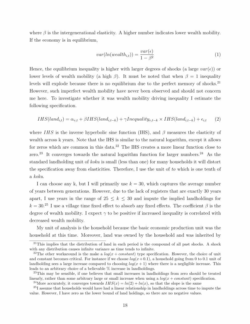
IHS(landi,t) = αv,t + βIHS(landi,t−k) + γInequalityv,t−k × IHS(landi,t−k) + εi,t (2)

where IHS is the inverse hyperbolic sine function (IHS), and β measures the elasticity of

wealth across k years. Note that the IHS is similar to the natural logarithm, except it allows

for zeros which are common in this data.22 The IHS creates a more linear function close to

zero.23 It converges towards the natural logarithm function for larger numbers.24 As the

standard landholding unit of koku is small (less than one) for many households it will distort

the specification away from elasticities. Therefore, I use the unit of to which is one tenth of

a koku.

I can choose any k, but I will primarily use k = 30, which captures the average number

of years between generations. However, due to the lack of registers that are exactly 30 years

apart, I use years in the range of 25 ≤ k ≤ 30 and impute the implied landholdings for

k = 30.25 I use a village time fixed effect to absorb any fixed effects. The coefficient β is the

degree of wealth mobility. I expect γ to be positive if increased inequality is correlated with

decreased wealth mobility.

My unit of analysis is the household because the basic economic production unit was the

household at this time. Moreover, land was owned by the household and was inherited by

21This implies that the distribution of land in each period is the compound of all past shocks. A shockwith any distribution causes infinite variance as time tends to infinite.

22The other workaround is the make a log(x + constant) type specification. However, the choice of unitand constant becomes critical. For instance if we choose log(x+ 0.1), a household going from 0 to 0.1 unit oflandholding sees a large increase compared to choosing log(x + 1) where there is a negligible increase. Thisleads to an arbitrary choice of a believable % increase in landholdings.

23This may be sensible, if one believes that small increases in landholdings from zero should be treatedlinearly, rather than some arbitrary large or small increase when using a log(x + constant) specification.

24More accurately, it converges towards IHS(x) = ln(2) + ln(x), so that the slope is the same25I assume that households would have had a linear relationship in landholdings across time to impute the

value. However, I have zero as the lower bound of land holdings, so there are no negative values.

18

All Villages Gini < 0.4 0.4 ≤ Gini ≤ 0.8 0.8 < GiniOut-Migration or Extinction 4.0 2.9 2.4 10.1

In-Migration 0.9 1.1 1.0 0.2

Branch Households 9.2 4.7 9.2 14.0

Observations 2936 558 1814 564

Table 5: The percentage composition of unobserved households, by village inequality level

Figure 10: Unobserved Observations

surviving members. Such units were mainly composed of family members although agricul-

tural servants would also be incorporated into the household at times. This unit of analysis

departs from the literature on social mobility which focus on individuals.26

One issue is household churn from movements in/out of the village or branching of house-

holds (see figure 5). Ignoring these households can lead to selection bias. In the case of

branching, whereby households split into the main and branch household, I assume both

households had the same landholdings as their parent’s generation.

Another issue is those that are truly unobserved (see figure 10). This is due to in/out-

migration or extinction. This happened in about 4% of cases. I cannot distinguish extinctions

and out-migrations in the data. If I assume leavers are similar to those who migrate in, I find

the median person moving into my village sample had zero land suggesting those households

have zero landholdings in the next period. Similarly out-migrants are disproportionately

26Individuals could potentially have very different outcomes compared to households. However an insightfulpaper by Kurosu and Ochiai (1995) suggests downward mobility was the norm for individuals.

19

(1) (2) (3) (4) (5) (6)

IHS(Landi,t−30) 0.292∗∗ 0.532∗∗∗ 0.360∗∗∗ 0.465∗∗∗ 0.560∗∗∗ 0.498∗∗∗

(0.127) (0.125) (0.101) (0.0755) (0.0672) (0.0558)

IHS(Landi,t−30) ∗Ginii,t−30 0.526∗∗∗ 0.212 0.424∗∗∗

(0.176) (0.166) (0.139)

IHS(Landi,t−30) ∗ CVi,t−30 0.0989∗∗∗ 0.0550∗∗ 0.0733∗∗∗

(0.0328) (0.0224) (0.0197)Famine No Yes Both No Yes Both

N 1440 1471 2911 1440 1471 2911adj. R2 0.532 0.640 0.590 0.531 0.642 0.591

Standard errors in parentheses∗ p < 0.1, ∗∗ p < 0.05, ∗∗∗ p < 0.01

Table 6: Inequality and MobilityCV denotes coefficient of variation. Robust standard errors. Villages are equally weighted.

from the poorest households. Thus, I assume they have zero landholdings.

The results are presented in table 6. There is a clear correlation between inequality

and intergenerational wealth mobility, whether I use the Gini coefficient or the coefficient

of variation. Going from an equal village in the data with a Gini coefficient of 0.3 to an

unequal village with a Gini coefficient of 0.8 increases the coefficient by 0.21. The results

are not explained by differing degrees of attenuation bias between the equal and unequal

regions as the difference in attenuation is less than 1% given my earlier estimates of the

measurement error.27 Since some of the data includes periods of famine one may worry

that this can distort mobility estimates. Therefore, if I only look at non-famine data, the

increase is higher at 0.26.28 Thus, the decrease in wealth mobility is extremely high. The

coefficient during famine becomes insignificant in the case of Gini coefficient, but remains

somewhat significant when using CV as the measure of inequality. These findings are robust

to using a specification with the natural logarithm (see Appendix table 9). One problem

with the results in table 6 is that the sample of villages in the famine and non-famine years

are different. This is advantageous, because I can look at a wider variety of villages and

have more power. However, if I limit the regression to the 11 villages for which both famine

and non-famine are observed, I can see if there are different dynamics during these different

times.

The results are shown in table . The magnitude of effects are similar during non-famine

27This is true even if I double my estimate of standard deviation of error to 28% of the value of land.28I define this as when the village does not see a famine from t− 30 to t

20

(1) (2) (3) (4) (5) (6)

IHS(Landi,t−30) 0.316∗∗ 0.738∗∗∗ 0.556∗∗∗ 0.438∗∗∗ 0.673∗∗∗ 0.556∗∗∗

(0.143) (0.155) (0.104) (0.0815) (0.0955) (0.0597)

IHS(Landi,t−30) ∗Ginii,t−30 0.520∗∗∗ -0.0592 0.184(0.190) (0.203) (0.141)

IHS(Landi,t−30) ∗ CVi,t−30 0.125∗∗∗ 0.0113 0.0647∗∗

(0.0352) (0.0403) (0.0266)Famine No Yes Both No Yes Both

N 708 791 1499 708 791 1499adj. R2 0.654 0.658 0.661 0.659 0.658 0.663

Standard errors in parentheses∗ p < 0.1, ∗∗ p < 0.05, ∗∗∗ p < 0.01

Table 7: Inequality and Mobility for Villages with data for both Famine and Non-famineYears.CV denotes coefficient of variation. Robust standard errors. Villages are equally weighted.

years, but the effect during famines are zero. Moreover, all villages appear to experience

an equal and low level of wealth mobility, with a coefficient of approximately 0.7. This is

suggestive of famines disrupting land markets and decreasing wealth mobility.

A Non-parametric Approach

The weakness of the parametric approach is that I assume a linear relationship between

past and future landholdings. However, the literature for modern day African societies have

found very different outcomes by wealth class. If there is some kind of poverty trap, I would

expect the poor and rich to have different rates of wealth mobility. Thus, an alternative

specification is the following.

IHS(Landholdingsi,t) = f(IHS(Landholdingsi,t−30) + εi,t

I estimate this using local polynomial smoothing. An issue is that landholdings have to have

the same value in all villages due to the regression looking at local effects at each landholding

level. This was not the case due to differing agricultural environments or tax rates. Yet,

single village regressions will lack power. Instead, I focus on regions that had similar socio-

economic environments namely the equal northeast and the unequal mino region of central

Japan.

I drop all branch households because they often got significantly less landholdings than

21

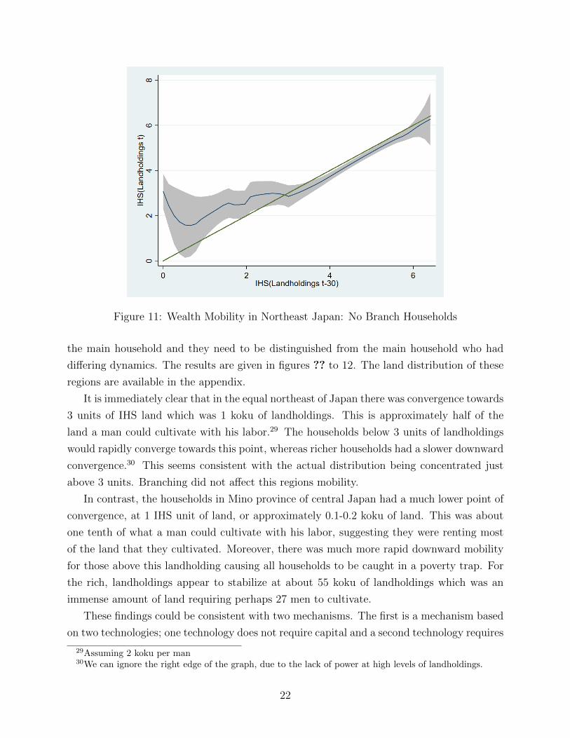
Figure 11: Wealth Mobility in Northeast Japan: No Branch Households

the main household and they need to be distinguished from the main household who had

differing dynamics. The results are given in figures ?? to 12. The land distribution of these

regions are available in the appendix.

It is immediately clear that in the equal northeast of Japan there was convergence towards

3 units of IHS land which was 1 koku of landholdings. This is approximately half of the

land a man could cultivate with his labor.29 The households below 3 units of landholdings

would rapidly converge towards this point, whereas richer households had a slower downward

convergence.30 This seems consistent with the actual distribution being concentrated just

above 3 units. Branching did not affect this regions mobility.

In contrast, the households in Mino province of central Japan had a much lower point of

convergence, at 1 IHS unit of land, or approximately 0.1-0.2 koku of land. This was about

one tenth of what a man could cultivate with his labor, suggesting they were renting most

of the land that they cultivated. Moreover, there was much more rapid downward mobility

for those above this landholding causing all households to be caught in a poverty trap. For

the rich, landholdings appear to stabilize at about 55 koku of landholdings which was an

immense amount of land requiring perhaps 27 men to cultivate.

These findings could be consistent with two mechanisms. The first is a mechanism based

on two technologies; one technology does not require capital and a second technology requires

29Assuming 2 koku per man30We can ignore the right edge of the graph, due to the lack of power at high levels of landholdings.

22

Figure 12: Wealth distribution in Mino Province, Central Japan: No Branch Households

capital (see figure ). Only farmers with sufficient capital or wealth can access this technology

due to borrowing constraints. Thus, there are two equilibria, A and B. Only household with

sufficient wealth to bring them beyond the switch point can converge towards B. Hence,

there is sharp downward mobility between A and the switch point as observed in the data.

This is consistent with the narrative that the central regions near the huge cities of Osaka,

Kyoto, and Nagoya used large amounts of fertilizer. This is likely due to demand for cash

crops such as cotton from being close to cities. Many plots were known to have been double

cropping, whereby two crops were cultivated in one year, and this required large amounts of

fertilizer to quickly replenish the soil. This was done in order to meet the demands of the

cities. The proximity to cities also had the advantage of having sufficient supply of fertilizer

from cities in the form of dried fish and night soil. Geographically, it was efficient for capital

intensive agriculture to be located near cities.

Within the qualitative literature, it has been found that fertilizer could take up 43%

of household expenditure.31 Such cultivation methods required huge amounts of wealth or

borrowing which must have been advantageous for rich households. On the other hand, such

conditions did not exist32 in northeast Japan and this may have resulted in one technology

and one equilibrium.

The other mechanism, which could have been simultaneously occurring, was that cottage

31Imai and Yagi (1955) 10432There is at least nothing in the qualitative literature that suggests widespread fertilizer use in this region.

23

Figure 13: Agricultural Production with Two Technologies

industry opportunities were more prevalent in the central region which were the centers of

commerce. Thus, the land poor households may have had other forms of wealth or skills

with which they could make up for their lack of wealth. Thus, they were content with being

landless households.

This dataset does not allow me to distinguish between these two mechanisms, and these

remain as hypothesis to study in future work.

Partible Inheritance and Extinction

Although wealth mobility was a significant factor in generating inequality, it fails to

capture changes in household composition. This is problematic if changes in household

composition were not random with respect to wealth. I focus on how household extinctions

(the disappearance of households from villages) and the formation of new households through

partible inheritance affected household wealth composition.

The positive correlation between incomes and fertility suggest household extinction would

be more common among the poor. Indeed, the poor were known to have difficulty finding

marriage partners and were less likely to have heirs. Extinctions rarely happened due to the

deaths of all household members. Instead it occurred due to households becoming non-viable

as economic units. For instance, a household with little landholdings and no laborers would

collapse as household members left the village for relatives.

One special factor which acted in favor of the rich were adult adoptions, as it prevented

the lack of biological heirs leading to extinction. In an insightful paper, Kurosu and Ochiai

24

Figure 14: Effects of Changes in Household Composition to Inequality

(1995) shows that almost no rich households went extinct due to adoptions. Despite the

roughly 17% chance that a household would have no male heir33, the social mechanism of

adoption allowed rich households to overcome biological barriers to household continuation.34

Against initial intuition, the lack of extinction among the rich due to adoption will

decrease inequality. This is due to the nature of inheritance for heir-less households. If the

landholdings go to a near relative in the event of the household having no heir, this leads

to the consolidation of wealth into the relative’s household. In contrast, the continuation of

rich households prevents wealth consolidation.

In the case of partible inheritace, a positive correlation between wealth and partible

inheritance would lead to lower inequality. This is because the rich are dispersing wealth

across households while the poorer households can sustain their wealth levels. The qualita-

tive literature suggests this was true, as a law limiting partible inheritance (bunchi seigen

rei) attempted to ban partible inheritance, except for land rich households35, effectively pro-

moting this mechanism. Figure 14 summarizes the effect of changing household composition

on inequality.

To estimate the effects of these mechanisms, I estimate the following specification,

Yi,t = βv + β1IHS(Landholdingsi,t−30) + β2IHS(Landholdingsi,t−30) ∗ inequalityi,t−30 + εi,t

33If one assumes 5 children with a 40% chance of death before adulthood.34This may have also caused more poor households to go extinct, as their sons got poached away. I thank

Fabian Drixler for pointing this out.35The definition of land rich differed by region, but a commonly stated threshold is 10 koku

25

Extinction Partible Inheritance(1) (2) (3) (4) (5) (6)

IHS(Landi,t−30) -0.143 -1.036∗∗∗ -0.527∗∗∗ 0.341 1.306∗∗∗ 0.758∗∗

(0.220) (0.308) (0.162) (0.369) (0.439) (0.299)

IHS(Landi,t−30) ∗Ginii,t−30 -0.232 0.764∗ 0.175 0.110 -1.027∗ -0.404(0.402) (0.409) (0.251) (0.534) (0.580) (0.409)

F-test for joint significance 8.36 34.92 44.55 21.43 28.46 44.41(p-value) (0.02) (0.00) (0.00) (0.00) (0.00) (0.00)

Famine? No Yes Both No Yes Both

N 499 946 1445 1389 1357 2746

Standard errors in parentheses∗ p < 0.1, ∗∗ p < 0.05, ∗∗∗ p < 0.01

Table 8: The Effect of Landholding on Household Inheritance & ExtinctionsA Logit Regression, with the marginal effects at the mean

where Yi,t denotes branching, partible inheritance, or extinction. Partible inheritance is

defined as cases in which branch households36 are observed with land in period t. I estimate

this using Probit or Logit regression. I expect β1 +β2 to be positive for partible inheritance,

and negative for extinctions.

The results for the logit regression are presented in table 37. Note that the sample size

changes due to some villages having no extinctions or partible inheritance. There is a general

negative correlation between landholdings and extinction but with an apparently larger effect

during famines. The overall effect is huge with the marginal effect of landholdings at the

mean being a 43% reduction in going extinct when looking at the whole sample38.

In the case of partible inheritance there is a positive correlation as expected. The effects

seem to be stronger during periods with famine. Again, the interaction term is not strongly

significant. The marginal effect at the mean is large with a 55% probability increase in

partible inheritance39. The inequality interaction term is never strongly significant showing

both mechanisms functioned uniformly across Japan and decreased inequality everywhere.

To get a sense of the magnitude of these effects, I plot the marginal effects of landholdings

by bin in Figure 15. It is clear that extinction was a small threat to the rich while at least

15% of the poorest household went extinct across each generation. In addition, partible

inheritance was also practiced predominantly by the rich who would split their wealth among

36branch households are all households that branched between t and t-3037The results using a probit regression are almost the same. See the appendix.38Assuming a household in a village with a Gini coefficient of 0.539Assuming a household in a village with a Gini coefficient of 0.5

26

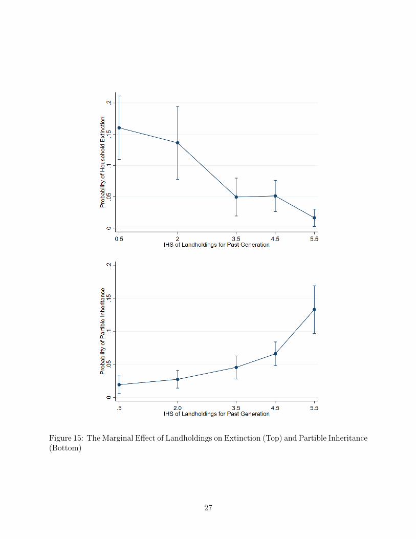
Figure 15: The Marginal Effect of Landholdings on Extinction (Top) and Partible Inheritance(Bottom)

27

multiple households at least 12% of the time while such cases were rare among the poorest.

The large magnitudes of these effects suggest this mechanism played a key role in reducing

inequality everywhere.

Conclusion

This paper is the first study that finds the “Great Gatsby Curve” relationship between

inequality and mobility in a pre-industrial economy. Much of the differences in inequality

across Japan can be explained by differing mobility patterns. In turn, the differing mobility

patterns appear to be explained by regional specialization in differing types of agriculture.

Areas near cities focused on capital intensive cash crops while the rural periphery focused on

labor intensive grains. Overall, mobility remains a key factor in explaining inequality among

agricultural societies.

The other big contribution has been to show that partible inheritance and extinction

could play a large role in inequality outcomes over the long-run. During an era in which

incomes and fertility were positively correlated, the extinction of the poor and the partible

extinction of the rich acted to reduce inequality within Japanese villages. If we compare

these findings to England circa 1600, extinction among the rich happened at least 20% of

the time among the richest households. This led to near relatives, who were also likely rich,

getting large transfers of wealth and increased inequality. This may partially explain why

Japan was a relatively equal society in the pre-industrial world. One implication is that

comparing differences in inheritance and extinction in addition to social mobility may give

us a more comprehensive idea of why inequality differs across societies.

Finally, the condition that favored equality in Japan was the positive correlation between

income and fertility but what would happen after the fertility transition. The implication

appears to be that there will be a reversal in effects with the rich going extinct and the

poor practicing partible inheritance leading to upward pressures on inequality. This could

be detrimental for growth if inequality affects education levels, as argued by De La Croix

and Doepke (2003). Could policies to decrease fertility in developing economies increasing

inequality and damage the chances for growth? This is a potential topic for future research.

28

Appendices

Alternative Specifications

(1) (2) (3) (4) (5) (6)

ln(Landi,t−30) 0.328∗∗∗ 0.569∗∗∗ 0.403∗∗∗ 0.481∗∗∗ 0.580∗∗∗ 0.515∗∗∗

(0.123) (0.118) (0.0976) (0.0735) (0.0642) (0.0544)

ln(Landi,t−30) ∗Ginii,t−30 0.480∗∗∗ 0.170 0.371∗∗∗

(0.172) (0.160) (0.136)

ln(Landi,t−30) ∗ CVi,t−30 0.0931∗∗∗ 0.0496∗∗ 0.0686∗∗∗

(0.0321) (0.0220) (0.0196)Famine No Yes Both No Yes Both

N 1440 1471 2911 1440 1471 2911adj. R2 0.542 0.683 0.607 0.542 0.684 0.608

Standard errors in parentheses∗ p < 0.1, ∗∗ p < 0.05, ∗∗∗ p < 0.01

Table 9: Inequality and Mobility, using natural logarithmRobust Standard Errors. Villages are equally weighted

Extinction Partible Inheritance(1) (2) (3) (4) (5) (6)

IHS(Landi,t−30) -0.0739 -0.546∗∗∗ -0.289∗∗∗ 0.178 0.619∗∗∗ 0.373∗∗∗

(0.120) (0.141) (0.0850) (0.172) (0.209) (0.139)

IHS(Landi,t−30) ∗Ginii,t−30 -0.121 0.415∗∗ 0.118 0.0477 -0.504∗ -0.208(0.207) (0.188) (0.127) (0.249) (0.272) (0.189)

F-test for joint significance 9.46 41.96 49.07 23.74 27.74 47.24(p-value) (0.01) (0.00) (0.00) (0.00) (0.00) (0.00)

Famine? No Yes Both No Yes Both

N 499 946 1445 1389 1357 2746

Standard errors in parentheses∗ p < 0.1, ∗∗ p < 0.05, ∗∗∗ p < 0.01

Table 10: The Effect of Landholding on Household Inheritance & ExtinctionsA Logit Regression with marginal effects at the mean

29

Wealth Distributions

Figure 16: Wealth distribution in Northeast Japan

Figure 17: Wealth distribution in Central Japan, Mino Province

30

References

Adermon, A., Lindahl, M., and Waldenstrom, D. (2018). Intergenerational wealth mobility

and the role of inheritance: Evidence from multiple generations. The Economic Journal,

128(612):F482–F513.

Alfani, G. (2015). Economic inequality in northwestern italy: a long-term view (fourteenth

to eighteenth centuries). The Journal of Economic History, 75(4):1058–1096.

Alfani, G. and Ammannati, F. (2017). Long-term trends in economic inequality: the case of

the florentine state, c. 1300–1800. The Economic History Review, 70(4):1072–1102.

Alfani, G. and Ryckbosch, W. (2016). Growing apart in early modern europe? a comparison

of inequality trends in italy and the low countries, 1500–1800. Explorations in Economic

History, 62:143–153.

Arimoto, Y. and Kurosu, S. (2015). Land and Labor Reallocation in Pre-Modern Japan: A

Case of a Northeastern Village in 1720-1870. IDE Discussion Paper.

Barrett, C. B. and Carter, M. R. (2013). The economics of poverty traps and persis-

tent poverty: empirical and policy implications. The Journal of Development Studies,

49(7):976–990.

Becker, G. S., Kominers, S. D., Murphy, K. M., and Spenkuch, J. L. (2018). A Theory of

Intergenerational Mobility. Journal of Political Economy, 126(S1):S7–S25.

Boserup, S. H., Kopczuk, W., and Kreiner, C. T. (2016). The role of bequests in shaping

wealth inequality: Evidence from danish wealth records. American Economic Review,

106(5):656–61.

Carter, M. R. and Barrett, C. B. (2006). The economics of poverty traps and persistent

poverty: An asset-based approach. The Journal of Development Studies, 42(2):178–199.

Carter, M. R. and Lybbert, T. J. (2012). Consumption versus Asset Smoothing: Testing the

Implications of Poverty Trap Theory in Burkina Faso. Journal of Development Economics,

99(2):255–264.

Cerman, M. (2012). Villagers and Lords in Eastern Europe, 1300-1800. Palgrave Macmillan.

Cinnirella, F. and Hornung, E. (2016). Landownership concentration and the expansion of

education. Journal of Development Economics, 121:135–152.

31

Clark, G. and Cummins, N. (2015). Intergenerational wealth mobility in england, 1858–2012:

Surnames and social mobility. The Economic Journal, 125(582):61–85.

Corak, M. (2013). Income Inequality, Equality of Opportunity, and Intergenerational Mo-

bility. Journal of Economic Perspectives, 27(3):79–102.

De La Croix, D. and Doepke, M. (2003). Inequality and Growth: Why Differential Fertility

Matters. American Economic Review, 93(4):1091–1113.

Drixler, F. (2013). Mabiki: infanticide and population growth in eastern Japan, 1660-1950,

volume 25. Univ of California Press.

Elinder, M., Erixson, O., and Waldenstrom, D. (2018). Inheritance and Wealth Inequality:

Evidence from Population Registers. Journal of Public Economics, 165:17–30.

Frankema, E. (2009). Has Latin America always been unequal?: a comparative study of asset

and income inequality in the long twentieth century, volume 3. Brill.

Hayami, A., Saito, O., and Toby, R. P. (2004). The Economic History of Japan: 1600-1990:

Volume 1: Emergence of Economic Society in Japan, 1600-1859. Oxford University Press.

Imai, R. and Yagi, A. (1955). Hoken Shakai no Noson Kozo. Yuhikaku.

Kraay, A. and McKenzie, D. (2014). Do poverty traps exist? assessing the evidence. Journal

of Economic Perspectives, 28(3):127–48.

Kurosu, S. and Ochiai, E. (1995). Adoption as an heirship strategy under demographic

constraints: A case from nineteenth-century japan. Journal of Family History, 20(3):261–

288.

Lybbert, T. J., Barrett, C. B., Desta, S., and Layne Coppock, D. (2004). Stochastic

wealth dynamics and risk management among a poor population. The Economic Journal,

114(498):750–777.

Mandai, Y. (2015). 19 seiki zenhan no jinushikeiei to kosakuninhensei. Shakai Keizai Shigaku,

81(1):69–93.

Matsuura, A. (2009). Shihai keitai to shumon aratame cho kisai: Echizen koku wo chushin

ni. Shodai Ronshu, 60(4):125–140.

Milanovic, B., Lindert, P. H., and Williamson, J. G. (2011). Pre-industrial inequality. The

economic journal, 121(551):255–272.

32

Saito, O. (2005). Wages, inequality and pre-industrial growth in japan, 1727-1894. Living

standards in the past, pages 77–97.

Saito, O. and Takashima, M. (2016). Estimating the shares of secondary-and tertiary-sector

outputs in the age of early modern growth: the case of japan, 1600–1874. European Review

of Economic History, 20(3):368–386.

Sellars, E. A. and Alix-Garcia, J. (2018). Labor Scarcity, Land Tenure, and Historical Legacy:

Evidence from Mexico. Journal of Development Economics, 135:504–516.

Takeyasu, S. (1966). Kinsei Hokensei no Tochi Kozo. Ochanomizu Shobou.

Takeyasu, S. (1969). Kinsei Kinai Nogyou no Kozo. Ochanomizu Shobou.

Watanabe, T. (1995). Kinsei Beisaku Tansaku Chitai no Sonraku Shakai: Echigokoku Iwa-

temura Satoke Monjyo no Kenkyu. Iwata Shoin.

Zimmerman, F. J. and Carter, M. R. (2003). Asset smoothing, consumption smoothing

and the reproduction of inequality under risk and subsistence constraints. Journal of

Development Economics, 71(2):233–260.

33