Explaining House Price Dynamics: Isolating the Role of Non-Fundamentals

Thao Le, National University of Singapore David Ling, University of Florida

Joseph Ooi, National University of Singapore

This paper was presented at Housing, Stability and the Macroeconomy: International Perspectives conference, November 14-15 2013. The conference was sponsored by the Federal Reserve Bank of Dallas, the International Monetary Fund, and the Journal of Money, Credit and Banking. The conference was held at Federal Reserve Bank of Dallas (http://dallasfed.org).

 

Explaining House Price Dynamics: Isolating the Role of Non-Fundamentals

David C. Ling, Joseph T.L. Ooi and Thao T.T. Le*

December 2011 Revised: November 8, 2013

Abstract

This paper examines the role of non-fundamentals-based sentiment in house price dynamics, including the well-documented volatility and persistence of house prices during booms and busts. To measure and isolate sentiment’s effect, we employ survey-based indicators that proxy for the sentiment of three major agents in housing markets: home buyers (demand side), home builders (supply side), and lenders (credit suppliers). After orthogonalizing each sentiment measure against a broad set of fundamental variables, we find strong and consistent evidence that the changing sentiment of all three sets of market participants predicts house price appreciation in subsequent quarters, above and beyond the impact of changes in fundamentals and market liquidity. More specifically, a one-standard-deviation shock to market sentiment is associated with a 22-80 basis point increase in real house price appreciation over the next two quarters. These price effects are large relative to the average real price appreciation of 0.71 percent per quarter observed over the full sample period. Moreover, housing market sentiment and its effect on real house prices is highly persistent. The results also reveal that the dynamic relation between sentiment and house prices can create feedback effects which contribute to the persistence typically observed in house price movements during boom and bust cycles. Keywords: Sentiment; housing prices; fundamentals

JEL Codes: R3, R21 * Ling: University of Florida; Ooi and Le: National University of Singapore. Acknowledgments: We thank Wayne Archer, Yuming Fu, Patric Hendershott, Yong Tu, Jiro Yoshida, as well as participants at the AREUEA National Meeting in Washington, DC (2011), the National University of Singapore research seminar (2011), and the Asian Real Estate Society Meeting in Kyoto, Japan (2013) for helpful comments and suggestions.

1  

Explaining House Price Dynamics: Isolating the Role of Non-Fundamentals

1. Introduction

The latest U.S. housing boom and bust has generated increased interest in the

dynamics of housing cycles. Most economists agree that house prices are determined in the

long-run by construction costs and economic fundamentals, such as household income,

population growth, employment, and interest rates (Min and Quigley 2006). However, despite

significant variation in hypotheses, modeling techniques, and data, much of the existing

empirical literature concludes that changes in the level and volatility of house prices and

price-to-rent ratios often exceed that which would be predicted by changes in economic

fundamentals (e.g., Duca, Muellbauer, and Murphy 2011; Gelain and Lansing 2013; Glaeser,

Gottlieb, and Gyourko 2013; Lai and Van Order 2010; Mikhed and Zemcik 2009; Shiller 2000).

For example, Glaeser, Gottlieb and Gyuorko (2013) conclude that interest rate declines explain

just 20 percent of the rise in house prices over the long 1996-2006 boom.

Although the standard fundamentals-based real user cost of housing model ignores the

availability of mortgage credit, a growing literature has reported evidence of a relation

between changes in underwriting standards, the supply of mortgage credit and subsequent

house price movement (e.g., Anderson, Capozza and Van Order 2011; Duca, Muellbauer, and

Murphy 2011, 2012; Mayer and Sinai 2009; Mian and Sufi 2009; and Taylor 2009).1 However,

measuring exogenous shifts in the mortgage credit supply function is challenging (Adelino,

Schoar, and Severione 2012 and Aron, et al. 2012). In fact, other researchers have argued that

credit availability and loan-to-value (LTV) ratios increased during the recent housing boom, at

least in part, because lenders were responding to increased home buyer optimism and

speculative demand for housing (Gelain and Lansing 2013; Dell’ Ariccia, Igan and Laeven

2012; and Goetzmann, Peng and Yen 2012).

Rather than attempting to find a causal relation between house price movements and

the availability of mortgage credit, this paper uses vector autoregression (VAR) models to

examine the dynamic short-run relation between real house prices and the “sentiment” of

three major agents in the U.S. housing market: potential home buyers (demand side), home

builders (supply side), and residential mortgage lenders (credit suppliers). Consistent with

Baker and Wurgler (2007), we define housing sentiment as a misguided belief about the                                                             1 The standard user cost of owner-occupied housing model is the discounted present value of after-tax mortgage payments and property tax payments, plus expected maintenance and capital expenditures, minus the expected net proceeds from the sale of the property at the end of the homeowner’s expected holding period.

2  

growth in housing prices, the risk of house price appreciation,2 or both, that cannot be justified

by the current economic information set available to housing market participants. In classical

finance models of asset pricing, there is no role for investor sentiment due to the rational

actions of informed arbitrageurs. However, in behavioral finance models, investor sentiment

can play a role in the determination of asset prices – independent of market fundamentals.3

The behavioral approach explicitly recognizes some investors and homeowners base

expectations on non-fundamental factors and that systematic biases in investors’ and

households’ beliefs can induce them to trade on non-fundamental information (i.e. sentiment).

It is important to note that a behavioral explanation for asset price movements also

requires “limits to arbitrage” in addition to sentiment-induced demand or supply. Examples of

limits to arbitrage that limit or preclude the ability of informed arbitragers to drive prices

back to their fundamental (intrinsic) levels include transaction costs, short-selling restrictions,

and “noise trader risk” (see De Long, et al. 1990). In housing markets, high transaction costs,

illiquidity, limited price revelation, and the inability to short-sell can prevent informed traders

from taking advantage of perceived profit opportunities. Consequently, housing prices may

diverge from their fundamental values for prolonged periods, consistent with the belief that

housing markets are less efficient than financial markets (Case and Shiller 1989).

Despite the potential role of sentiment in explaining house price movements, no

research of which we are aware has tested directly the dynamic relation between measures of

market-wide sentiment and house price dynamics. Instead, sentiment is often inferred

indirectly as price deviations from fundamental values (Mayer 2011). For example, Abraham

and Hendershott (1996) use the difference between actual metropolitan house price levels and

a “fundamental” price level to explain large subsequent declines in real house prices. However,

the inability to observe fundamental housing values makes it difficult to attribute observed

deviations to actual mispricing or model misspecification.

After orthogonalizing each of our survey-based sentiment measures against a broad set

of fundamental variables, we relate each to quarterly changes in real house prices at the

national and MSA level over the 1990Q2-2010Q3 period. A key implication of many models of

                                                            2 Cochrane (2008) argues that it is difficult to distinguish between an asset price bubble and a situation in which rational investors have low risk premiums, and therefore low discount rates and user costs of capital. We define a risk premium as being too low (i.e., non-rational) if its level is inconsistent with current economic fundamentals, including the risk premiums available to households on alternative investments of similar risk. 3 Fama (1988) and Hirsheifer (2001) provide a non-real estate focused review from the rational camp and the behavioral side, respectively. Scherbina and Schlusche (2011) provide a more recent survey of the literature on asset pricing bubbles.

3  

real estate price dynamics (e.g., Burnside et. Al. 2013) is that booms (busts) are associated

with increases (decreases) in liquidity. We therefore include a proxy for market liquidity as a

third endogenous variable in our VAR models. To the extent housing sentiment and market

liquidity are correlated, the inclusion of a liquidity proxy in our empirical models helps avoid a

potential missing variable problem and its attendant bias. Sentiment, including shifts in the

willingness of lenders to extent mortgage credit, is clearly not exogenous. However, by

modeling the dynamic relation between sentiment, house prices, and market liquidity

(turnover) in a VAR framework, we are able to quantify feedback effects among the three

endogenous variables while controlling for their potential endogeneity.

Our primary results can be summarized as follows. First, we find consistent evidence

that high levels of sentiment predict greater house price appreciation in subsequent quarters,

all else equal. A one-standard-deviation shock to, respectively, home buyer, builder, and lender

sentiment is associated with a 22 to 80 basis point increase in real house price appreciation

over the next two quarters. These price effects are large relative to the average real price

appreciation of 0.71 percent per quarter observed over the full sample period. Moreover,

sentiment’s effect on house prices in subsequent quarters persists over a sustained period of

time, which is consistent with the well documented momentum in house price movements.

Second, we find consistent evidence that increased price appreciation predicts significantly

higher levels of sentiment in subsequent quarters among home buyers and mortgage lenders.

Homebuilders, however, do not appear to be backward-looking in forming their expectations.

These results are robust to the addition of a fourth endogenous variable that controls for the

potential endogeneity of demand and supply driven sentiment.

We also perform a MSA-level analysis using the price appreciation indices of the MSAs

tracked by the Case-Shiller Index. Sinai (2012) finds that individual housing markets in the

U.S. have experienced considerable heterogeneity in the amplitude and timing of their house

price cycles. However, we find that national level sentiment proxies are a significant predictor

of price appreciation in 17 of the 19 MSAs. Thus, our national results are not driven by a small

set of MSAs.

Our results are also robust to a number of alternative specifications, including

replacing the individual sentiment indices with a composite sentiment index, using sales

volume in place of turnover as a proxy for market liquidity, and using the Federal Housing

Finance Agency (FHFA) house price index in place of the S&P/Case-Shiller index to measure

house price appreciation. We also test sentiment’s effect over different sub-periods and find

4  

that house prices are more sensitive to changes in market liquidity and past price changes

during boom and bust periods.

We also perform in-sample forecasts of price appreciation to compare the accuracy of

our models to a benchmark model that does not include a sentiment index. Overall, models

that incorporate a measure of sentiment have lower forecast errors than the benchmark

model. Finally, we estimate the long-run effects of sentiment using an overlapping price

change regression model. The estimated coefficients on sentiment are positive and significant

in the one, two, and three-year predictive price appreciation regressions, indicating a 

continuation of price divergence from fundamental values for as long as three years.

Overall, our results provide strong and consistent support for the hypothesis that U.S.

house prices are driven, at least in part, by changes in non-fundamentals-based sentiment

among housing market participants. The results also reveal that the dynamic relations among

sentiment, house prices, and market liquidity can create feedback effects which contribute to

the persistence typically observed in house price movements during boom and bust cycles.

The remainder of the paper proceeds as follows: Section 2 reviews the related

literature; Section 3 describes our sentiment proxies; Section 4 explains the empirical

methodology employed; Section 5 discusses the selection and summary statistics of our

exogenous fundamental control variables; Section 6 contains the empirical results, including a

number of robustness checks. Finally, Section 7 summarizes our findings and their

implications.

2. Literature review

The seminal work of Case and Shiller (1989) on housing market inefficiency has been

followed by a large stream of literature focused on the serial correlation and forecastability of

housing prices. Recently, Glaeser et al. (2011) calibrate a dynamic rational expectations model

to reconcile three stylized facts about housing prices that have puzzled researchers: high

volatility, serial correlation, and mean reversion. Although their model is able to explain mean

reversion and price volatility over one-year horizons, it substantially underpredicts price

volatility over time horizons longer than a year; moreover, it fails to account for the observed

serial correlation (persistence) in house prices.

The authors offer two explanations for their findings. First, serial correlation in house

prices may be the result of a learning process during which households and other market

participants only gradually infer the level of housing demand from transaction prices. The

5  

second, less rational, explanation is the extrapolation hypothesis; that is, market participants

with myopic expectations infer future house price changes from past price changes. This

explanation is consistent with recent findings on household’s expectations of future house

price appreciation. As noted by Jurgilas and Lansing (2013), this survey-based evidence can

be a useful tool for detecting nonfundamentals-based expectations. For example, using survey

data from 2002 and 2003, Case and Shiller (2003) found that respondents expected house

prices to increase 12 to 16 percent per year over the next ten years, implying more than a

three-fold increase in house prices. Case, Shiller, and Thompson (2012) presents conclusions

from a panel survey conducted by the authors in four major U.S. cities (Alameda, Boston,

Milwaukee and Orange).4 The authors conclude that “12-month expectations [of future house

price changes] are fairly well described as attenuated versions of lagged actual 12-month price

changes.”5 The mean-reverting “anchor” placed on housing prices in the long-run by

construction costs appeared to have little or no role in the formation of home buyer price

appreciation expectations.

Using the Michigan Survey of Consumers, Piazzesi and Schneider (2009) report that

“starting in 2004, more and more households became optimistic after having watched house

prices increase for several years.” Using data from the same survey, Lambertini, Mendicino

and Punzi (2012) document that news about recent changes in business conditions can

significantly affect consumers' belief of favorable buying conditions in the housing market.

Moreover, both news on business conditions and expectations of rising house prices and future

tighter credit conditions are significantly related to house price growth. These findings are

consistent with their hypothesis on expectations-driven cycles in the housing market.

Dua (2008) also uses the Michigan Survey of Consumers to identify the factors

influencing homebuyers’ perceptions. Interest rates, income, wealth, financial status and

current house prices are found to Granger-cause home buying attitudes, among which interest

rates play the most influential role. Interestingly, impulse response functions show that rising

prices predict increased sentiment in the short run, but negative sentiment over longer

horizons. However, Dua (2008) does not model the possibility of a reverse causality from

sentiment to house prices.

                                                            4 The first survey was conducted in 1988. The authors replicated it in 2003, 2005 and each year from 2005 through 2012. 5 In a recent study on 36 countries from 2005 to 2012, Aizenman and Jinjarak (2013) also find that the most important factor accounting for real estate price appreciation is the impact of momentum. They conclude that the concerns of Shiller (2000) regarding irrational exuberance apply globally.  

6  

Overall, this survey-based evidence suggests home buyers are more likely to

extrapolate past house price trends than to base decisions on the discounted present value of

the expected service flow, or the real, after-tax user cost, of housing. More formally, recent

research has shown that models with moving-average expectations outperform rational, or

fundamentals-based, models in predicting asset prices, including housing prices. For example,

Gelain and Lansing (2013) demonstrate that the inclusion of moving-average forecast rules for

a subset of market participants can significantly magnify house price appreciation and

volatility in a standard dynamic stochastic general equilibrium model. Simulations performed

by Granziera and Kozicki (2012) show that a rational expectations model is unable to explain

the recent boom and bust in house prices, whereas asset pricing models with backward-

looking expectations are able to capture observed house price changes and volatility during the

2000s.6

Acknowledging the shortcomings of fundamentals-based models in explaining housing

boom-bust cycles, Burnside et al. (2013) introduce a model in which housing market

participants have heterogeneous expectations about long-term fundamentals. Moreover, these

agents interact with each other. These “social dynamics” produce changes in the fraction of

agents who are optimistic about long-run fundamentals and these changes can induce non-

trivial dynamics into house prices. Their model attributes a key role to buyers with speculative

motives. That is, booms (busts) are characterized by increases (decreases) in the proportion of

agents who buy homes primarily because of large expected price appreciation.

Although it appears backward-looking, non-fundamentals-based expectations and

social dynamics help explain housing booms and busts, Glaeser, Gottlieb and Gyourko (2013)

point out that little is known about the process that creates and sustains non-fundamentals-

based expectations, including simple moving-average forecasts. Moreover, the authors suggest

that understanding the role played by non-fundamentals-based “sentiment” in setting price

appreciation expectations is a pressing research topic.

In addition to the literature focused on the formation of price appreciation expectations

and the serial correlation and forecastability of housing prices, the latest housing boom and

bust has produced a growing literature on the role of eroding mortgage underwriting

                                                            6 As pointed out by Gelain and Lansing (2013), the adoption of a backward-looking forecast rule “can be viewed as boundedly-rational because it economizes on the costs of collecting and processing information.” For this reason we avoid the use of the term “irrational” and instead define sentiment as the portion of house price appreciation expectations not based on economic fundamentals.    

7  

standards and the dramatic increase in the market share of subprime loans. (Duca,

Muellbauer and Murphy 2011; Duca, Muellbauer and Murphy 2012; Haughwout et al. 2011;

Himmelberg, Mayer and Sinai 2005; Hubbard and Mayer 2009; Mayer and Pence 2009; Mayer

and Sinai 2009; Mian and Sufi 2009; Taylor 2009). Duca Muellbauer and Murphy (2011) show

that incorporating an accurate measure of LTV ratios for first-time home buyers into models of

price-to-rent ratios yields stable long-run relationships, more precisely estimated effects,

reasonable speeds of adjustment, and improved model fits. Duca, Muellbauer and Murphy

(2012) also report a causal relation between swings in mortgage credit standards and house

price movement during the recent boom and bust.

Mayer and Sinai (2009) show that the growth in subprime lending was greatest in

housing markets that experienced the most dramatic increases in price-rent ratios. Mayer and

Pence (2009) further document that the median loan-to-value ratio was 100 percent for

subprime mortgages originated in 2005, 2006, and the first half of 2007. Anderson, Capozza

and Van Order (2011) and Dell’Ariccia, Igan and Laeven (2012) find that the lower

underwriting standards during this period contributed largely to the credit boom and its

ensuing crisis. Favilukis, Ludvigson and Van Nieuwerburgh (2012) apply an asset-pricing

model to explain fluctuations in the price-rent ratios between 2000 and 2007. The authors

conclude that the observed volatility in price-rent ratios is a rationally expected response to

the changes in residential mortgage markets; in particular, the relaxation of credit

constraints, during their study period.7 Finally, Mora (2008) finds evidence that increased

bank lending fuelled the Japanese real estate boom in the 1980s, with every 0.01 increase in

real estate loans as a share of total loans leading to 14 to 20 percent higher land inflation.

In short, there is growing empirical evidence that the traditional fundamentals-based

user cost of capital model, which includes the cost, but not the availability, of mortgage credit,

is unable to explain observed movements in house prices, especially during boom and bust

periods. We now turn to an examination of whether the inclusion of measures of non-

fundamentals-based housing sentiment improve our ability to explain real house price changes

and changes in market liquidity and, secondly, whether house price changes are predictive of

future levels of sentiment and liquidity. That is, do sentiment, house prices, and liquidity

interact to produce sustain periods of mispricing?

                                                            7 However, the paper takes no stand on whether the changes in housing finance can be characterized as a rational response to economic conditions and/or regulatory changes.  

8  

3. Measures of Housing Sentiment

Several proxies of investor sentiment have been developed for public equity markets.8

These sentiment indicators can be broadly categorized as either direct or indirect measures.

Indirect proxies for investor sentiment are abstracted from a set of quantifiable market

indicators believed to proxy, at least in part, for market sentiment. These include closed-end

fund discounts, trading volume, mutual fund flows, and the volume of IPOs and SEOs. In

contrast, direct sentiment measures are derived from surveys of market participants, such as

the UBS/Gallup surveys of randomly-selected investor households, Investor’s Intelligence

surveys of financial newsletter writers, and the University of Michigan Survey of Consumers.9

We construct direct measures of sentiment using surveys of home buyers, home builders, and

mortgage lenders in the U.S. These agents represent, respectively, the demand, supply, and

financial intermediary sectors of the U.S. housing market. We are not aware of prior research

that provides a comprehensive examination of the role played by each of these housing market

agents.

The sentiment of potential and current home buyers is captured by the Survey of

Consumers, which is conducted monthly by the Survey Research Center at the University of

Michigan (http://www.sca.isr.umich.edu/). For each monthly survey, approximately 500

households from all states in the U.S. are chosen using a rotating panel sample design.10 Each

survey contains approximately 50 core questions to track consumers’ attitudes and

expectations about personal finances, business conditions, and buying conditions.11 Souleles

(2004) finds that the sentiment data from this survey are useful in predicting households’

consumption expenditure. The Index of Consumer Expectations, produced from the survey, is

included in the Leading Indicator Composite Index published by the U.S. Department of

Commerce, Bureau of Economic Analysis.

                                                            8 Baker and Wurgler (2007) provide a comprehensive discussion of the various proxies for investor sentiment in the stock market. Investor sentiment in securitized real estate markets has been the subject of several studies.

9 Qiu and Welch (2005) provide a comparison of several direct survey-based measures of investor sentiment.

10 See http://www.sca.isr.umich.edu/for more details on sample design.

11 Personal finances are addressed in questions about expected change in nominal as well as real family income. Attitudes towards business conditions in the economy are measured using questionnaire concerning expected changes in inflation, unemployment, interest rates, and confidence in government economic policies. Finally, there are several questions probing for the respondent's appraisal of buying conditions for large household durables, vehicles, and houses (see http://www.sca.isr.umich.edu/).

9  

We use the following survey question that addresses respondents’ attitudes about home

buying conditions: “Generally speaking, do you think now is a good time or a bad time to buy a

house?” The responses fall into three broad categories: “good,” “bad,” and “uncertain.” The

follow-up question asks respondents to provide reasons for their previous answers, which are

then classified into six groups for the “good” response and four groups for the “bad” response.

The six reasons for the “good” response include: “prices will increase,” “prices low,” “interest

rates low,” “rising interest rates,” “good investment,” and “time’s good.” We use the percentage

of respondents who think it is a “good” time to buy “because price will increase” as our

sentiment proxy for households (BUYER). This percentage captures changes in the proportion

of households who are bullish about the housing market due to their expectations of large

capital gains (Burnside et al. 3013). .

We use the NAHB/Wells Fargo Housing Market Index published by the National

Association of Home Builders (NAHB: www.nahb.org) to measure the perceptions of U.S.

homebuilders. Derived from a survey conducted monthly by NAHB since 1985, this index

captures the opinions of approximately 400 builders regarding three metrics of housing

market conditions: (1) current sales of new single-family homes, (2) expected sales of new

single-family homes over the next six months, and (3) traffic of prospective buyers in new

homes. The respondents are asked to rate their perceptions of current and expected sales as

"good," "fair," or "poor," and the traffic of prospective buyers as “high-to-very-high,” “average,”

or “low-to-very-low.” The final Housing Market Index (BUILDER) is a weighted average of the

three component indices, where weights are based on their correlations with single-family

housing starts.12 The index can range from zero to 100, with an index number over 50

indicating that more builders view sales conditions as good than poor. BUILDER is widely

interpreted by NAHB and industry watchers as an indicator of “builder confidence.”

Our measure of credit suppliers’ opinions about housing markets is obtained from the

Federal Reserve Board’s Senior Loan Officer Opinion Survey on Bank Lending Practices (see

www.federalreserve.gov). This is a quarterly survey of approximately sixty large domestic

banks and twenty-four US branches or agencies of foreign banks. The purpose of the survey is

to provide qualitative and limited quantitative information on credit availability and demand,

                                                            12 The three component indices are calculated by applying the formula [(Good - Poor + 100)/2] to the present and future sales series, and [(High/Very High-Low/Very Low + 100)/2] to the traffic series. This puts each index on a zero to 100 scale. The indices are then seasonally adjusted (http://www.nahb.org/generic.aspx?sectionID=134& genericContentID=532).

10  

as well as evolving developments and lending practices in the U.S. loan markets.13 The survey

has maintained consistency in its core set of questions since the second quarter of 1990; this

dictates the beginning of our sample period. Responses to this survey have been used as a

proxy for credit availability in the private equity market (Franzoni et al. 2012), debt market

constraints in leveraged buyouts (Axelson et al. 2012), and the supply of loans available to

public corporations (Leary 2009), and the availability of credit in commercial real estate

markets (Ling, Naranjo, and Scheick 2013).

We focus on responses to the following question: “Over the past three months, how have

your bank's credit standards for approving applications from individuals for mortgage loans to

purchase homes changed?” Respondents must select one of the following: “tightened

considerably,” “tightened somewhat,” “remained essentially unchanged,” “eased somewhat,” or

“eased considerably.” We posit that changes in lending standards for home mortgages reflect

the banks’ changing perspectives about the riskiness of the housing markets.14 We use the net

percentage of banks easing their standards (i.e., the percentage of banks easing their

standards minus the percentage of banks tightening their standards) as our proxy of lender

sentiment (LENDER). It is important to emphasize that changes in house prices likely affect

market sentiment. That is, we are not arguing that a sentiment-pricing spiral is initiated by

an exogenous shock to sentiment. Instead, we model the interaction between house prices and

sentiment, as well as market liquidity, in a VAR model that allows all three variables to be

treated as endogenous.

BUYER, BUILDER and LENDER are likely to be correlated with economic factors such

as GDP and income per capita.15 As discussed by Brown and Cliff (2005), when market

participants report they are bullish on the market, it may be a rational projection of

                                                            13 Survey questions focus on two broad areas: changes in the demand for credit and changes in bank lending policies. Various types of loans are covered in the survey, including commercial and industrial loans, commercial real estate loans, residential real estate loans, and consumer lending. In addition, a portion of the questions in each survey cover special topics of timely interest, such as the securitization of mortgage loans and the financial crisis.

14 Take the 2010Q4 survey as an example. The top three reasons cited by the respondents for their tightening of credit standards for commercial and industrial loans include: “less favorable or more uncertain economic outlook,” “reduced tolerance of risk,” and “increased concerns about the effects of legislative changes, supervisory actions, or changes in accounting standards.” Conversely, banks easing their credit standards for commercial and industrial loans cited “more favorable or less uncertain economic outlook,” “improvement in industry-specific problems,” and “more aggressive competition from other banks or nonbank lenders” as their motivation. Apparently, banks take into account their outlook for the riskiness of specific markets. Although there is no survey question to address the reasons for changing credit standards for home mortgage loans, it is reasonable to believe banks are motivated by similar factors when making loans to the residential market.

15 For example, the contemporaneous correlations of BUYER, BUILDER and LENDER with real GDP growth over our sample period are 0.28, 0.54, and 0.55, respectively.

11  

prosperous times to come, a projection not justified by the set of fundamental information

currently available, or some combination of the two. Following Baker and Wurgler (2007), we

orthogonalize our three sentiment series against a set of macroeconomic variables to remove

the influence of fundamentals. The macroeconomic factors used in the orthogonalization

regressions include U.S. population growth, GDP growth, growth in household income, change

in the unemployment rate, and the change in the mortgage lending rate. In our VAR analysis,

we use the residuals from these three regressions as our proxies for buyer, builder, and lender

sentiment. As a robustness test, we also use principal component analysis to extract a

composite sentiment index from the three orthoganalized indices.

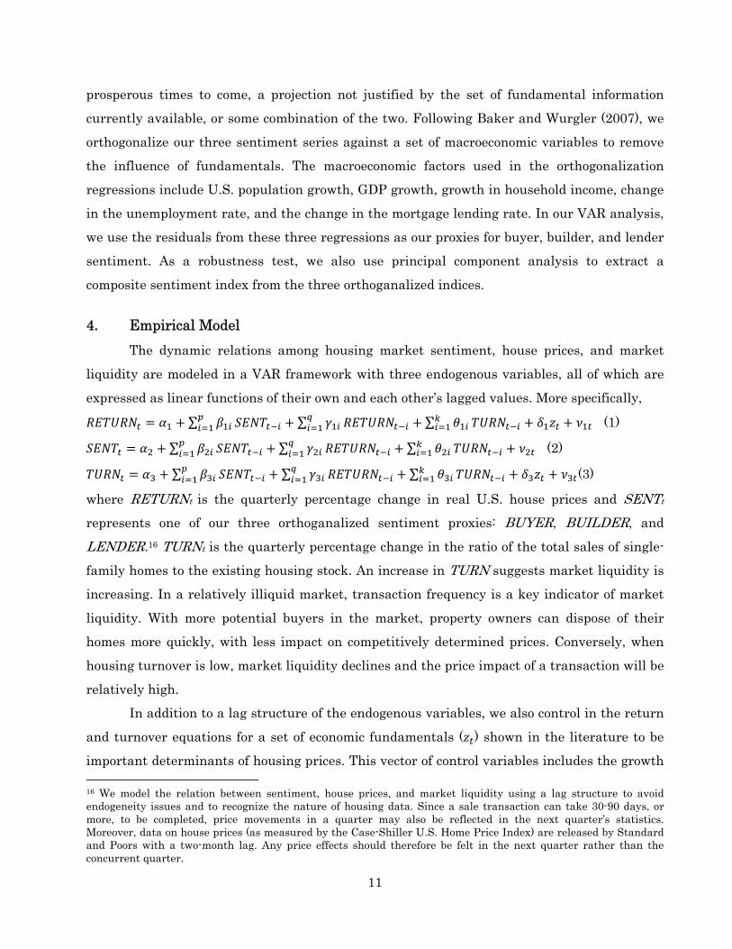
4. Empirical Model

The dynamic relations among housing market sentiment, house prices, and market

liquidity are modeled in a VAR framework with three endogenous variables, all of which are

expressed as linear functions of their own and each other’s lagged values. More specifically,

∑ ∑ ∑ (1)

∑ ∑ ∑ (2)

∑ ∑ ∑ (3)

where RETURNt is the quarterly percentage change in real U.S. house prices and SENTt

represents one of our three orthoganalized sentiment proxies: BUYER, BUILDER, and

LENDER.16 TURNt is the quarterly percentage change in the ratio of the total sales of single-

family homes to the existing housing stock. An increase in TURN suggests market liquidity is

increasing. In a relatively illiquid market, transaction frequency is a key indicator of market

liquidity. With more potential buyers in the market, property owners can dispose of their

homes more quickly, with less impact on competitively determined prices. Conversely, when

housing turnover is low, market liquidity declines and the price impact of a transaction will be

relatively high.

In addition to a lag structure of the endogenous variables, we also control in the return

and turnover equations for a set of economic fundamentals ( ) shown in the literature to be

important determinants of housing prices. This vector of control variables includes the growth                                                             16 We model the relation between sentiment, house prices, and market liquidity using a lag structure to avoid endogeneity issues and to recognize the nature of housing data. Since a sale transaction can take 30-90 days, or more, to be completed, price movements in a quarter may also be reflected in the next quarter’s statistics. Moreover, data on house prices (as measured by the Case-Shiller U.S. Home Price Index) are released by Standard and Poors with a two-month lag. Any price effects should therefore be felt in the next quarter rather than the concurrent quarter.

12  

in the population of individuals between 20 and 30 years of age (POP), real GDP growth

(GDP), real per capita income growth (INCOME), the change in the unemployment rate

(UNEMP), the change in the real mortgage interest rate (MGTRATE), and the change in the

number of newly completed housing units (SUPPLY). Changes in the control variables are

measured from quarter t-1 to t. The vector of controls is not included in the SENT equation

because the three sentiment proxies have been orthoganalized with respect to the variables

included in . Maximum Likelihood Estimation (MLE) is employed to simultaneously

estimate equations (1), (2), and (3) using quarterly data over the 1990Q2 - 2010Q3 sample

period.

We are primarily interested in the estimated coefficients on lagged sentiment in the

RETURN regression ( ). The impact of market sentiment on housing prices is arguably

through the demand side, at least in the short run. When potential buyers believe prices are

very likely to rise, they are more willing to make housing investments because of less

perceived risk and/or high potential price appreciation.17 However, the VAR system specified

above allows for feedback to exist among all three endogenous variables: sentiment, house

prices, and market liquidity.

Riddel (1999) posits that once price begins to increase, positive feedback traders enter

the market in search of momentum profits and accentuate the rise; in contrast, during periods

of price declines feedback traders exacerbate price movements through their selling activities.

During the early stages of the recent house price boom and bust, Case and Shiller (2003) find

that many homebuyers based their purchase decisions, at least in part, on their fear of being

unable to afford a home if they delayed their purchase. Moreover, many financial

intermediaries shared these optimistic expectations of future house price increases and may

have contributed to the rapid appreciation by reducing their lending standards.

Evidence of price changes affecting sentiment suggests myopic expectations and return

chasing behavior. When prices are increasing (decreasing), myopic market participants believe

prices will continue to increase (decrease). If home buyers and lenders chase price

appreciation, the estimated coefficients on in equation (2) are expected to be positive.

Moreover, the dynamic relation between sentiment and home prices may “spiral,” with one

                                                            17 The two major types of buyers that will be highly motivated include (1) first-time homebuyers who act swiftly for fear of being priced out of the market, and (2) speculators who search for excess returns from the price momentum. These optimistic buyers will further be encouraged with easier and cheaper access to credit if developers and creditors share the same optimism. As a result, the market will experience an increase in speculative demand, driving prices away from fundamental values. The reverse can occur in pessimistic periods.

13  

change reinforcing the other. The illiquidity, limits to arbitrage, and information asymmetry

that characterize housing markets also render them more susceptible to pricing spirals,

thereby potentially extending the length and magnitude of cycles.

5. Data

We use the percentage change in the real Case-Shiller U.S. National Home Price Index

(nominal index deflated by the CPI-less-shelter) to measure quarterly house price appreciation

( . The Case-Shiller U.S. National Home Price Index is a composite price index for

single-family homes from all nine U.S. Census divisions, released quarterly by Standard and

Poors (see www.standardandpoors.com). The index is constructed using the repeat sale

methodology refined by Case and Shiller (1989).

Both the University of Michigan Survey of Consumers and the NAHB builder survey

are conducted monthly, while the FED survey of lenders is conducted quarterly. To

synchronize the different frequencies, our subsequent analyses are conducted on a quarterly

basis using the Survey of Consumer and NAHB indices for the months of March (Q1), June

(Q2), September (Q3), and December (Q4), respectively.

Descriptive statistics for our endogenous variables are reported in Table 1. Over the

study period, real house prices registered an average quarterly appreciation rate of 0.71

percent. Both the maximum (5.07 percent in 2005Q1) and the minimum (-8.68 percent in

2009Q1) real appreciation rates occurred during the recent boom and bust period. BUYER,

BUILDER, and LENDER are well-behaved mean-zero indices, as they are residuals obtained

from regressing the original series against a set of fundamental factors. The serial correlation

of BUYER, BUILDER, and LENDER are 0.52, 0.82, and 0.72, respectively. Clearly, even our

orthoganalized sentiment indices are highly persistent.

Figure 1 plots BUYER, BUILDER, and LENDER against contemporaneous real house

price changes over the 1990:Q2-2010:Q3 study period. Among the three indices, BUYER

(Panel A) is the least correlated with real house price movements, especially during the 1995-

2005 period when housing returns and the other two sentiment indices exhibit a consistent

upward trend. BUYER, in contrast, seems to move rather erratically during the 1995-2005

period. This observation is confirmed by the contemporaneous correlation between real house

price changes and BUYER (Table 3), which is a statistically insignificant 0.21. In contrast, the

correlation between real house price changes and BUILDER and LENDER is 0.55 and 0.61,

respectively.

14  

The change in the ratio of total home sales to the existing housing stock, TURN, has a

quarterly mean of -0.05 and a standard deviation of 5.32. TURN displays no significant serial

correlation. VOLUME, our alternative measure of market liquidity, is defined as the change in

the total sales of new and existing single-family homes. VOLUME has a quarterly mean of

0.37 and displays significant time variation but no significant serial correlation.

Descriptive statistics for our macroeconomic control variables are reported in Table 2. 

The quarterly data were obtained from various sources including the Bureau of Economic

Analysis, Bureau of Census, and Bureau of Labor Statistics. All macroeconomic controls are

specified as changes from quarter t-1 to t. The estimation of VARs with nonstationary

variables may produce spurious regression results. We therefore test for stationarity of our

regression variables. The results of these Dickey-Fuller tests, as reported in the last column of

Table 1and Table 2, confirm that all variables are stationary.

The contemporaneous correlations among our endogenous variables are reported in

Table 3 and reveal that our sentiment indices are positively and significantly correlated. Given

our orthoganalization procedure, we can be confident that our sentiment proxies capture

expectations that are independent of fundamental macroeconomic factors. This allows us to

interpret the estimated sentiment coefficients as the marginal effect of sentiment on house

prices. It is interesting to note that BUYER and LENDER are uncorrelated with TURN and

VOLUME. Interestingly, however, BUILDER is positively correlated with TURN and

VOLUME, suggesting that builder sentiment is shaped directly by home sales.

6. Results

6.1 Base Model

Table 4 contains results from the estimation of our trivariate VAR models with

RETURN, SENT, and TURN as endogenous variables. Although the coefficient estimates are

not reported, we also include in the RETURN and TURN equations the change from quarter t-

1 to t in the set of control variables listed in Table 2. This three-equation VAR specification

allows us to test for feedback effects among changes in sentiment, market liquidity, and house

prices, while also controlling for changes in fundamentals. The sample period is 1990:Q2 to

2010:Q3. Conventional lag-length selection criteria (AIC, HBIC, and SBIC) indicate that four

lags of all endogenous variables are most appropriate for the models specified. The first set of

equations in Table 4 corresponds to the use of our buyer sentiment index, the second set

15  

[equations (4) through (6)] corresponds to our builder sentiment model, and the last set

[equations (7) through (9)] to our lender sentiment model.

To examine the cumulative effects of the four lags of our endogenous variables, we sum

the estimated lagged coefficients and test for joint significance. The summed coefficients and

F-stats associated with tests of joint significance are reported in parentheses in Table 4.18

Controlling for lagged price returns, lagged turnover, and changes in fundamentals,

increased sentiment over the prior four quarters predicts more real house price appreciation in

the buyer, builder, and lender models. These sentiment effects are economically as well as

statistically significant. Consistent with several earlier studies that find that changes in

consumer sentiment are predictive of changes in real consumer spending (Carroll, Furher, and

Wilcox 1994; Howrey 2001; Ludvigson 2004; Souleles 2004), especially discretionary

expenditures (Curtin 1982), our results confirm that optimism (pessimism) on the part of

homebuyers can translate into real changes in the demand for houses and thus drive prices up

(down).19 Interestingly, changes in builder confidence also predict price movements beyond

what fundamentals would suggest. Finally, banks play a crucial role in accommodating the

buying and selling activities of the other two market players through credit channels20. As

observed in the recent subprime mortgage crisis, overly optimistic banks may loosen their

credit standards in boom periods and thereby help to fuel price increases (Duca et al. 2011;

Duca et al. 2012; Haughwout et al. 2011; Mian and Sufi 2009)21.Taken together, these findings

strongly support our main hypothesis that sentiment is an important determinant of house

price dynamics. That is, the well-documented high volatility of house prices compared with

observable changes in fundamentals can be ascribed, at least in part, to shifts in housing

market sentiment.

The sum of the four lagged coefficients on TURN is positive and highly significant in

each of the three RETURN equations. That is, lagged market liquidity is highly predictive of

                                                            18 The estimated coefficients on all lagged endogenous variables and their individual significance levels are available upon request from the authors. 19 Curtin (1982) argues that discretionary expenditures that involve large purchases, such as houses, vehicles, or large durables, requires active planning and decision making on the part of consumers. Such expenditure therefore depend not only on income, prices, interest rate, and other traditional market variables, but also on the attitudes of the decision makers and their expectations of future developments. 20 However, one challenge associated with analyzing the effect of changes in builder and lender sentiment on house price changes is disentangling the supply and demand channels. We discuss this issue in the next section. 21 Ramcharan and Crowe (2013) provide an examination of the reverse impact from house price fluctuations to the availability of credits.

16  

house price changes. However, we find no evidence that lagged returns predict turnover. In

contrast, we find strong evidence that increases in buyer and builder sentiment are associated

with increased turnover in subsequent quarters. Each of our three model specifications

explains approximately 78 percent of the variation in quarterly real house price appreciation.

The impulse response functions (IRFs) associated with these VAR estimations are

displayed in Figure 2. These IRFs trace the impact of a one-standard-deviation shock to the

orthoganalized sentiment variables on subsequent house price appreciation. A positive shock

to buyer, builder and lender sentiment, respectively, produces a 30.6, 0.9 and 16.0 basis point

increase in real house price appreciation in the next quarter. The price responses rise further

by 50.7, 21.4 and 39.2 basis points, respectively, in the second quarter. In total, a standard-

deviation sentiment shock is associated with a cumulative price increase of 22-80 basis points

over the next three quarters. Given that the average real price change over the sample period

is 0.71 percent per quarter (Table 1), these price responses are economically significant.

The IRFs also reveal that sentiment’s effects on house prices are highly persistent; a

one standard deviation shock to any of the three sentiment indices appears to influence real

price changes for as long as 10 quarters. This protracted price effect reflects the highly illiquid,

segmented and informationally inefficient characteristics of housing markets, as well as the

lack of a short-sale market. With some initial stimulating condition, such as an abundance of

easy credit, the sentiment-induced mispricing inherent in house prices can spiral into a

bubble. These findings provide at least a partial answer to the question raised by Glaeser,

Gottlieb, and Gyourko (2013) about the interplay among price changes, expectations, and

credit conditions.

We next turn to the three SENT equations in Table 4 for evidence of feedback effects;

that is, from house price movements to sentiment. The sum of the four lagged RETURN

coefficients in the buyer model is positive and highly significant in the sentiment equation (F-

stat=14.7). Households, presumably the least sophisticated and most informationally

constrained agents in the market, appear to rely on past price movements to form their non-

fundamentals-based expectations of future house price movements. Past house price

movements also predict changes in lender sentiment [equation (8)]. Coupled with the

persistent impact of sentiment on house prices established above, this finding of a positive

feedback loop from prices to buyer and lender sentiment may help explain the increased

persistence and volatility of house price changes during boom and bust periods. In contrast,

builder sentiment does not appear to be backward looking [equation (5)]. This finding is

17  

consistent with the results reported by Glaeser, Gyourko, and Saiz (2008), who show that

developers lead rather than follow house price movements.

6.2 Models Including both Demand and Supply Driven Sentiment Proxies

Home buyer sentiment is expected to impact house prices primarily through a demand

channel. In contrast, our measures of home builder and lender sentiment are expected to work

primarily through housing supply and credit supply channels. One challenge associated with

analyzing the effect of changes in home builder and lender sentiment on house prices is

isolating the supply-side channel from potential demand-side determinants. For example, if

lenders cater mortgage lending decisions to shifts in home buyer sentiment, an observed

relation between changes in lender sentiment and house prices may in fact be driven in part

by speculative home buyer demand. Similarly, if home buyer sentiment responds positively to

increases in the availability of mortgage credit, an observed relation between home buyer

sentiment and house price movements may be driven in part by increased credit availability.

To control for the potential endogeneity of demand and supply driven sentiment, we also

estimate several versions of a four equation VAR model that includes both demand- and

supply-side sentiment proxies.

We estimate a four equation VAR model that includes buyer sentiment (BUYER) in

addition to lender sentiment (LENDER), along with lagged real price appreciation and

turnover, to control for the potential endogeneity of demand and supply driven sentiment.

Although not separately tabulated, the sum of the four lagged coefficients on BUYER in the

RETURN regression is positive and highly significant, as expected. However, the inclusion of

BUYER as a fourth endogenous variable in the VAR does not alter the positive relation

between lagged lender sentiment and house price appreciation in the current quarter. The

sum of the four lagged coefficients on LENDER remains positive and significant at the one

percent level (F-stat = 15.95); moreover the sum of the four lagged coefficient on LENDER

increases somewhat in magnitude with the addition of BUYER to the model. Said differently,

controlling for a demand-side sentiment channel does not mitigate the strong positive relation

detected between lagged LENDER and RETURN.

We also estimate a four equation VAR model that includes buyer sentiment (BUYER)

in addition to builder sentiment (BUILDER), along with lagged real price appreciation and

turnover. Again, the inclusion of BUYER as a fourth endogenous variable in the VAR does not

alter the positive relation between lagged builder sentiment and current quarter house price

18  

appreciation. Overall, these results strongly suggest that our consistent finding of a significant

role for builder and lender sentiment in predicting house price appreciation is not due to the

omission of an omitted demand-side variable (channel).

6.3 Composite Sentiment Index

As reported in Table 3, our three sentiment indices are correlated. Thus, it is likely

they have a common sentiment factor that can be extracted using principal component

analysis. We therefore construct a composite direct sentiment index (PCSENT) as the first

principal component of the three series, similar to Baker and Wurgler (2007). The descriptive

statistics for PCSENT is reported in Table 1.

As displayed in Figure 3, PCSENT tracks the overall trend of real house price changes

relatively well; in fact, the two time series have a contemporaneous unconditional correlation

of 0.60 over the sample period. Table 5 reports the results of estimating our trivariate VAR

model using PCSENT as our sentiment proxy. Based on standard selection criteria, the

appropriate lag-length for this alternative model is again four lags of the endogenous

variables.

Our central finding from the individual survey-based measures of sentiment is

strengthened by the use of the composite index. Increases in lagged sentiment are strongly

associated with subsequent real house price appreciation. Lagged market liquidity remains

highly predictive of house price changes and increases in PCSENT are associated with

increased turnover in subsequent quarters. The associated impulse response function

displayed in Figure 4 confirms that the impact of PCSENT on house price appreciation is both

economically significant and highly persistent; a one-standard-deviation positive shock to

PCSENT is associated with a 66 basis-point increase in real house price appreciation over the

next two quarters.

We also estimated our three-equation VAR model using trading volume, VOLUME, in

place of TURN as a proxy for market liquidity. PCSENT is again used as our sentiment proxy.

Four lags of each endogenous variable, as indicated by standard selection criteria, are also

included. Although not separately tabulated, the sum of the four lagged coefficients on

PCSENT is positive and highly significant in the RETURN equation. Thus, controlling for

trading volume in place of housing turnover does not alter our basic findings.

To summarize, our VAR analysis strongly suggests that the sentiment of important

agents in housing markets is associated with house price appreciation in subsequent quarters.

19  

Moreover, this pricing effect is highly persistent. Changes in market liquidity are also highly

predictive of house price appreciation, indicating the importance of a liquidity channel as well

as a sentiment (i.e., demand) channel. We also find strong evidence of backward-looking

expectations of future real price changes among households and weaker evidence among

lenders. The dynamic interplay among sentiment, house prices, and liquidity appear to be a

self-reinforcing process, which provides a potential explanation for the susceptibility of

housing markets to price persistence and volatility.

6.4 Additional Robustness Tests

To test the robustness of our results, we use the quarterly house price index published

by the Federal Housing Finance Agency (FHFA) in place of the S&P/Case-Shiller index to

measure real house price appreciation. The FHFA index measures the price movements of

single-family detached houses for all nine U.S. Census Divisions. Both the S&P/Case-Shiller

index and the FHFA index are constructed using the repeat-sale methodology. However, the

FHFA index is estimated from transactions involving conforming, conventional mortgages

purchased or securitized by Fannie Mae or Freddie Mac. It therefore excludes single-family

homes purchased with non-conforming mortgages, such as jumbo, Alt-A, and subprime

mortgages. In contrast, the S&P/Case-Shiller index is constructed from transaction data

obtained from county assessor and recorder offices, with no restrictions on the type of

financing. Additionally, the S&P/Case-Shiller index is value-weighted while the FHFA index

is equally-weighted.

Table 6 contains results from estimating our trivariate VAR using the FHFA index to

measure house price movements. We use our composite sentiment index (PCSENT). Most

importantly, lagged changes in PCSENT remain highly predictive of real house price changes.

The sum of the four lagged coefficients on TURN is also positive and significant at the 5

percent level in the RETURN equation. In addition, increases in lagged sentiment are

associated with increased turnover in subsequent quarters. However, lagged house price

appreciation no longer predicts sentiment.

To compare sentiment’s effect in different market conditions, we re-estimate our VAR

models using two sub-periods: a pre-housing boom (or normal) market and a boom and bust

market. Naturally, an important step in this test is identifying the start of the recent housing

boom period. Since there is no clear theoretical guide to define the beginning of a boom, we

follow the empirical approach used by Ferreira and Gyourko (2011). They describe the

20  

structural breakpoint or, in other words, a significant discrete jump in the growth rate of

house prices, as signaling the onset of a house price boom. More specifically, we identify the

quarter during which there is a global structural break by estimating the following equation: ∗ for 1 < < 61 (4)

where is the real price change in quarter t; is the intercept term; measures the

importance of the potential breakpoint; ∙ is an indicator function which equals 1 if its

condition is true, and 0 otherwise; is quarter t; ∗ is the location of the potential structural

break, and is the error term. The structural breakpoint ( ∗ is the quarter that maximizes

the R2 of the equation; that is, the quarter in which the change in price growth has the highest

power in explaining the price growth series itself. We estimate the regression using data from

1990Q2 (t=1) to 2005Q1 (t=61) to avoid any influence of the recent boom period in locating the

structural breakpoint.22

The highest R2 achieved from the estimation of equation (4) is 59.4 percent at 1998Q1,

indicating it is the quarter when the structural break occurred. Graphically, it can also be

observed from Figure 1 and 3 that price appreciation prior to 1998Q1 fluctuates around 0.5%;

after 1998Q1, it averages approximately 2.5% per quarter. We therefore split our study period

into two sub-periods, 1990Q2-1997Q4 and 1998Q1-2010Q3, and report the two sets of VAR

results in Table 7.

Prior to the start of the boom (1990Q2-1997Q4), lagged turnover and lagged house

prices changes are not significantly related to current real house price movements. The

significant effect of lagged sentiment on current house prices is, however, still evident. Thus,

an importance inference from these subsample results is that there appears to be a sentiment-

induced mispricing component in house prices, regardless of market conditions. Another

noteworthy result is that, in the second sub-period, sentiment seemed to gather momentum

such that it could be largely predicted by its previous values (Column 5, R2 = 0.801); In

contrast, sentiment levels during the first sub-period cannot be explained by either past

market liquidity or past sentiment levels (Column 2, R2 = 0.373). These results suggest that

house prices are more sensitive to changes in market liquidity and past prices during boom

and bust periods. In addition, sentiment also becomes more predictable.

To further analyze the role of sentiment in housing markets, we perform an in-sample

forecast of price appreciation to evaluate the accuracy of our estimated RETURN equation

                                                            22 We choose 2005Q1 because it is the quarter with the highest real price changes (RETURN). Thereafter, price appreciation started to slow.

21  

compared to a benchmark model that includes all of the explanatory variables except a

sentiment proxy. Model (5) below incorporates both our fundamental and sentiment variables,

while Model (6) contains only the fundamental variables. More specifically,

∑ ∑ ∑ (5)

∑ ∑ (6)

The backward test involves estimating the two models on the full sample period and

using the estimated coefficients to dynamically forecast house price changes between 1998Q1-

2010Q3. Specifically, the estimated coefficients and actual historical values of the exogenous

right-hand-side variables are fitted to the models, except for the autoregressive price changes

(i.e., ) where the previous period’s forecasts are used instead of actual data. This

approach allows us to judge how well the different models can replicate historical data; in

particular, the house price movements during the boom and bust of the recent housing cycle

(1998Q1-2010Q3).

Figure 5 also plots the actual and forecasted values of RETURN from equations (5) and

(6). Three common measures of forecast accuracy -- mean error (ME), mean percentage error

(MPE), and mean squared error (MSE) -- are reported in Table 8. Overall, the model that

incorporates the sentiment index (Model 5) provides a more accurate forecast of price

appreciation; i.e. it has a lower forecast error than the benchmark model as measured by all

three criteria. This result is consistent with prior research (e.g., Granziera and Kozicki 2012)

that suggests house price models that account for the role of non-fundamentals, in addition to

fundamental factors, have better predictive power.

6.5 MSA-Level Analysis

Our analyses to this point have been carried out using price appreciation data at the

national-level. To further examine the robustness of our results, we repeated the analysis

using the (real) price appreciation rates of the 19 MSAs tracked by the S&P/Case-Shiller

indices over our study period 1990-2010.23 Sorting the MSAs based on their real price

appreciation over the study period, the local housing markets in 12 of the 19 MSAs recorded

positive real returns, whilst the remaining seven markets experience net declines in real

house prices between 1990 and 2010.

For each market, we run VAR models using local MSA price appreciation, national

turnover, national sentiment (PCSENT) and national macroeconomic variables. Although not

                                                            23 The Case-Shiller Index for Dallas is not included in the analysis because it is not available prior to 2000. 

22  

separately tabulated, the estimation results show that national sentiment predicts local house

price changes. Specifically, the sum of the lagged coefficients on PCSENT is positive and

significant at the 1 percent level in 17 of 19 MSAs; thus, our national results are not driven by

a few MSAs.24 Moreover, national housing market sentiment matters in local markets, even

after controlling for past price appreciation in the MSA.

In 11 of the 14 Case-Shiller MSAs that experienced price appreciation over the sample

period, the estimated coefficient on RETURN in the sentiment equation is positive and

significant; that is MSA level returns predict national sentiment. It is only in the five worst

performing markets, where price appreciation was actually negative over our sample period,

that MSA-level returns do not predict national sentiment. We also find that national-level

turnover does not predict MSA price appreciation, which is consistent with MSA-level returns

being predicted by local, rather than national, transaction activity.

6.6 Long-Run Regressions

The discussion to this point has focused mainly on the short-run dynamic relation

between house prices and market sentiment through a VAR framework. Arguably, if periods of

optimism (pessimism) lead to house prices overshooting (undershooting) in the initial periods,

the market should observe a negative relationship between cumulative long-run returns and

sentiment as house prices revert to their fundamental values over time.

In this section, the long-run effect of sentiment is tested using a framework adapted

from Brown and Cliff (2005). This framework involves regressing future k-period quarterly

real housing returns on a vector of control variables and our composite sentiment index,

:

⋯ / (7)

where , … , are quarterly real price changes as before, k is the number of

quarters in the holding period return, is the intercept term, is the same set of control

variables employed in the previous VAR models, and is the composite sentiment

index derived from the homebuyers’, builders’ and lenders’ sentiment measures. The test is

carried out for one- to five-year horizons (k = 4 to 20). If sentiment’s effect is persistent, as one

would expect in the housing markets, this will result in a positive coefficient on over

a short and medium horizon that is similar to the results from the VAR models. However,

                                                            24In Las Vegas, the coefficient is positive, but only significant at the 10% level. Only in Boston is the coefficient on PCSENT not significant.

23  

market prices should eventually revert to their fundamental values, such that a negative

coefficient on in the long run will be observed.

There are two econometric issues in estimating the long-run model specified above.

Firstly, the use of overlapping observations in the dependent variable results in a moving

average process in the error term, causing the standard errors obtained from an OLS

estimation to be biased downwards. The second issue is the potential finite sample bias in the

coefficient estimate of a persistent independent variable (in this case, the coefficient

associated with the sentiment index ( ). Stambaugh (1999) shows that a persistent

explanatory variable, though predetermined, is not strictly exogenous. Although an OLS

estimate is consistent and asymptotically normally distributed under the predetermined

assumption, it might suffer from biasness with a finite sample setting. To address these

econometric issues, we employ a bootstrap simulation procedure similar to Brown and Cliff

(2005) and Ling, Naranjo and Scheick (2013). The details of the bootstrap procedure are

explained in Appendix A.

Table 9 reports the bias-adjusted coefficients of the sentiment measure and

their standard errors for the five return horizons. The results are revealing. The sentiment

coefficients on the one-, two- and three-year average returns are significantly positive,

indicating a continuation of price divergence from fundamental values for as long as three

years. However, their magnitudes are decreasing as the return horizon increases, which points

towards a gradual price correction process at work.

The effect of sentiment then falls sharply in both economic and statistical significance

in the four-year return regression, and becomes insignificant over the five-year horizon. These

results strongly suggest that market sentiment at a given time induces very persistent

mispricing in future house prices that takes beyond five years to correct. It is consistent with

the empirical findings in previous sections that housing markets are highly susceptible to

prolonged periods of sentiment-induced mispricing. The five-year adjustment period is a

marked contrast to the quick correction of stock prices in studies such as Schmeling (2009),

Barber, Odean and Zhu (2009), and Brown and Cliff (2005) who find that stock prices revert

in one to twelve months. It is, on the other hand, close to the results from prior studies in the

housing literature that examine the response of prices to supply and demand shocks. For

example, Harter-Dreiman (2004) finds that it takes about five years for house prices to get

within 70 percent of the new equilibrium value in response to an income shock; the

adjustment time estimated by Malpezzi (1999) is approximately 10 years. Examining the rent-

24  

price ratio using 355 years of data on the Amsterdam housing market, Ambrose, Eichholtz and

Lindenthal (2013) conclude from their vector error correction results that the market

correction of mispricing can take decades.25 Nevertheless, a potential limitation of our findings

is that the recent housing boom and bust is a significant portion of our study period (1990Q2-

2010Q3). Thus, the slow correction found in the long-run regression may be driven partly by

the fact that house prices were consistently rising for a significant percentage of the sample.

7. Conclusion

The current study is the first of which we are aware to test directly the dynamic

relation between market-wide sentiment and real house price change. The primary

contribution of the study is the use of a set of proxies that capture the consensus sentiment of

three major agents in housing markets: homebuyers (demand side), home builders (supply

side), and lenders (financial intermediaries). To directly test the role of sentiment in housing

markets, we relate each sentiment proxy (after orthogonalization with respect to

macroeconomic fundamentals) to quarterly changes in real house prices over the 1990Q2-

2010Q3 study period using a three-equation vector autoregression (VAR) model that also

includes a measure of market liquidity as a third endogenous variable. We find strong and

consistent evidence that housing market sentiment predicts real house price appreciation in

subsequent quarters, above and beyond the impact of lagged price appreciation, lagged market

liquidity, and changes in a broad set of fundamentals. More specifically, a one-standard-

deviation shock to sentiment is associated with a 22-80 basis point increase in real house price

appreciation over the next two quarters. These price impacts are large relative to the average

real price appreciation of 0.71 percent per quarter observed over the full sample period.

Moreover, this pricing effect is highly persistence.

We also find that changes in market liquidity consistently predict house price changes;

moreover changes in sentiment are positively associated with market liquidity in the

subsequent quarters. Thus, sentiment appears to affect house prices directly, as well as

indirectly through a market liquidity channel. We also find strong evidence of backward-

looking expectations of future house price changes among households and weaker evidence

among lenders.

                                                            25 The authors contend that since mispricing can persist for a long period, bubble crashes are not always inevitable in the short run. It is hence difficult to know when, or even if, a bubble will collapse. The price correction process may take the form of a fading out over decades than a sudden crash.

25  

Our results are robust to a number of alternative specifications, such as replacing the

individual sentiment indices with a composite sentiment index, using sales volume in place of

turnover as a proxy for market liquidity, and using the Federal Housing Finance Agency

(FHFA) house price index in place of the S&P/Case-Shiller index to measure house price

appreciation. We also test sentiment’s effect over different sub-periods and find that house

prices are more sensitive to changes in market liquidity and past price changes during boom

and bust periods.

We also perform in-sample forecasts of price appreciation to compare the accuracy of

our models to a benchmark model that does not include a sentiment index. Overall, models

that incorporate a measure of sentiment have lower forecast errors than the benchmark

model. We repeat the analysis using MSA-level house price appreciation in place of the

national-level returns. The estimation results show that national sentiment predicts MSA-

level house price changes; thus, our national results are not driven by a few MSAs. Finally, we

also estimate the long-run effects of sentiment using an overlapping price change regression.

The estimated coefficients on sentiment are positive and significant in the one, two, and three-

year predictive price appreciation regressions, indicating a continuation of price divergence

from fundamental values for as long as three years.

In sum, our results provide strong and consistent support for the hypothesis that house

prices are affected by changes in sentiment among important market participants. The results

also reveal that the dynamic interplay between sentiment and house prices can create a self-

reinforcing spiral, which provides a potential explanation for the susceptibility of housing

markets to price persistence and volatility.

References  

Abraham, J. M. and Hendershott, P. H. (1996). “Bubbles in Metropolitan Housing Market”. Journal of Housing Research, 7(2), 191-207.

Adelino, M., A. Schoar, and F. Severino. (2012). “Credit Supply and House Prices: Evidence from Mortgage Market Segmentation.” NBER Working Paper.

Aizenman, J. and Y. Jinjarak (2013). “Real Estate Valuation, Current Account, and Credit Growth Patterns Before and After the 2008-2009 Crisis.” ADBI Working Paper 429. Tokyo: Asian Development Bank Institute.

Ambrose, Brent W., Piet Eichholtz, and Thies Lindenthal. (2013) "House Prices and Fundamentals: 355 Years of Evidence." Journal of Money, Credit and Banking, 45, 477-491.

Anderson, Charles D., Dennis R. Capozza, and Robert Van Order. (2011) "Deconstructing a Mortgage Meltdown: A Methodology for Decomposing Underwriting Quality." Journal of Money, Credit and Banking, 43, 609-631.

26  

Aron, Jannie, John V. Duca, John Muellbauer, and Keiko. (2012) “Credit, Housing Collateral, and Consumption: Evidence from Japan, the U.K.,and the U.S.” Review of Income and Wealth 58, pgs. 397-423.

Axelson, Ulf, Tim Jenkinsom, Per Stromberg, and Michael Steven Weisbach. (2012) "Borrow Cheap, Buy High? The Determinants of Leverage and Pricing in Buyouts." NBER Working Paper.

Baker, Malcolm, and Jeffrey Wurgler. (2007) "Investor Sentiment in the Stock Market." Journal of Economic Perspectives, 21, 129-151.

Barber, Brad M., Terrance Odean, and Ning Zhu. (2009) "Do Retail Trades Move Markets?" The Review of Financial Studies, 22, 151-186.

Brown, Gregory W., and Michael T. Cliff. (2005) "Investor Sentiment and Asset Valuation." The Journal of Business, 78, 405-440.

Burnside, Craig, Martin Eichenbaum, and Sergio Rebelo. (2013) “Understanding Booms and Busts in Housing Markets.” Working paper.

Carroll, C., J. Fuhrer, and D. Wilcox. (1994) “Does Consumer Sentiment Forecast Household Spending? If So, Why?”American Economic Review, 84(5),1397-1408.

Case, Karl E., and Robert J. Shiller. (1989) "The Efficiency of the Market for Single-Family Homes." The American Economic Review, 79, 125-137.

Case, Karl E., and Robert J. Shiller. (2003) "Is There a Bubble in the Housing Market?" Brookings Papers on Economic Activity, 2, 300-361.

Case, Karl E., Robert J. Shiller, and Anne Thompson. (2012) "What Have They Been Thinking? Home Buyer Behavior in Hot and Cold Markets." NBER Working Paper Series No. 18400.

Cochrane, John H. (2008). “The Dog that Did Not Bark: A Defense of Return Predictability.” Review of Financial Studies 21, 1533-1575.

Curtin, Richard T. (1982). “Indicators of Consumer Behavior: The University of Michigan Surveys of Consumers.” The Public Opinion Quarterly, 46(3), 340-352

Dell’Ariccia, Giovanni, Deniz Igan, and L. U. C. Laeven. (2012) "Credit Booms and Lending Standards: Evidence from the Subprime Mortgage Market." Journal of Money, Credit and Banking, 44, 367-384.

De Long, J. Bradford, Andrei Shleifer, Lawrence H. Summers, and Robert J. Waldmann. (1990). “Noise Trader Risk in Financial Markets”. Journal of Political Economy, 98: 703-738.

Dua, Pami. (2008) "Analysis of Consumers’ Perceptions of Buying Conditions for Houses." The Journal of Real Estate Finance and Economics, 37, 335-350.

Duca, John H., John Muellbauer, and Anthony Murphy. (2011) “House Prices and Credit Constraints: Making Sense of the U.S. Experience.” The Economic Journal 121: 533-551.

Duca, John H., John Muellbauer, and Anthony Murphy. (2012) “Shifting Credit Standards and the Boom and Bust in U.S. House Prices: Time Series Evidence from the Past Three Decades.” Working paper.

Fama, Eugene F. (1998) "Market efficiency, long-term returns, and behavioral finance." Journal of Financial Economics, 49, 283-306.

Favilukis, Jack, Sydney C. Ludvigson, and Stijn V. Nieuwerburgh. (2010) "The Macroeconomic Effects of Housing Wealth, Housing Finance, and Limited Risk-Sharing in General Equilibrium." NBER Working Paper No. 15988.

Ferreira, Fernando, and Joseph Gyourko. (2011) "Anatomy of the Beginning of the Housing Boom: U.S. Neighborhoods and Metropolitan Areas, 1993-2009." NBER Working Paper Series No. 17374.

27  

Franzoni, Francesco, Eric Nowak, and Ludovic Phalippou. (2012) "Private Equity Research Performance and Liquidity Risk." The Journal of Finance, 67, 2341-2373.

Gelain, Paolo and Keving J. Lansing. (2013) “House Prices Expectations, and Time-Varying Fundamentals.” Working paper, Norges Bank Research.

Glaeser, Edward L., Joshua D. Gottlieb, and Joseph Gyourko. (2013) "Can Cheap Credit Explain the Housing Boom?" In Housing and the Financial Crisis, edited by E. Glaeser and T. Sinai.

Glaeser, Edward L., Joseph Gyourko, Eduardo Morales, and Charles G. Nathanson. (2011) "Housing Dynamics." Working Paper.

Glaeser, Edward L., Joseph Gyourko, and Albert Saiz. (2008) "Housing supply and housing bubbles." Journal of Urban Economics, 64, 198-217.

Goetzmann, William N., Liang Peng and Jacqueline Yen. (2012) “The Subprime Crisis and House Price Appreciation.” Journal of Real Estate Finance and Economics, 44, 36-56.

Granziera, Eleonora, and Sharon Kozicki. (2012) "House Price Dynamics: Fundamentals and Expectations." Working Paper.

Harter-Dreiman, Michelle. (2004) "Drawing inferences about housing supply elasticity from house price responses to income shocks." Journal of Urban Economics, 55, 316-337.

Haughwout, Andrew, Donghoon Lee, Joseph Tracy, and Wilbert van der Klaauw. (2011) "Real Estate Investors, the Leverage Cycle, and the Housing Market Crisis." Federal Reserve Bank of New York Staff Report No. 514.

Himmelberg, Charles, Christopher Mayer, and Todd Sinai. (2005) "Assessing High House Prices: Bubbles, Fundamentals and Misperceptions." The Journal of Economic Perspectives, 19, 67-92.

Hirshleifer, David. (2001) "Investor Psychology and Asset Pricing." The Journal of Finance, 56, 1533-1597.

Howrey, E. P. (2001) “The Predictive Power of the Index of Consumer Sentiment.” Brookings Papers on Economic Activity, 1, 175–207.

Hubbard, Glenn R., and Christopher J. Mayer. (2009) "The Mortgage Market Meltdown and House Prices." Journal of Economic Analysis and Policy, 9.

Jurgilas, Marius and Kevin J. Lansing. (2013) “Housing Bubbles and Expected Returns to Homeownership: Lessions and Policy Implications.” Available at SSRN: http//ssrn.com/abstract=2209719.

Lai, Rose N. and Robert A. Van Order. (2010) “Momentum and House Price Growth in the United States: Anatomy of a Bubble.” Real Estate Economics 38, 753-773.

Lambertini, Luisa, Maria T. Punzi , and Caterina Mendicino. (2012) "Expectations-Driven Cycles in the Housing Market." Bank of Finland Research Discussion Paper No. 2/2012.

Leary, Mark T. (2009) "Bank Loan Supply, Lender Choice, and Corporate Capital Structure." The Journal of Finance, 64, 1143-1185.

Ling, David C., Andy Naranjo, and Benjamin Scheick. (2013) "Investor Sentiment, Limits to Arbitrage, and Private Market Returns.” Real Estate Economics, Vol. 41, No. 2 (2013).

Ludvigson, S. C. (2004) “Consumer Confidence and Consumer Spending.” Journal of Economic Perspectives, 18(2), 29–50.

Malpezzi, Stephen. (1999) "A Simple Error Correction Model of House Prices." Journal of Housing Economics, 8, 27-62.

Mayer, Christopher. (2011) "Housing Bubbles: A Survey." Annual Review of Economics, 3, 559-577.

Mayer, Christopher, and Karen Pence. (2009). "Subprime Mortgages: What, Where, and to Whom?" In Housing Markets and the Economy: Risk, Regulation, and Policy edited by Glaeser EL, and Quigley JM, pp 149-196. Cambridge, MA: Lincoln Land Inst.

28  

Mayer, Christopher, and Todd Sinai. (2009). "U.S. House Price Dynamics and Behavioral Economics." In Policy Making Insights on Behavioral Economics edited by Foote CL, Goette L, and Meier S, pp 261-295. Boston: Fed. Reserve Bank Boston.

Mian, Atif, and Amir Sufi. (2009) "The Consequences of Mortgage Credit Expansion: Evidence from the U.S. Mortgage Default Crisis." Quarterly Journal of Economics, 124, 1449-1496.

Mikhed, Vyacheslav, and Petr Zemcik. (2009) “Do House Prices Reflect Fundamentals? Aggregate and panel data evidence.” Journal of Housing Economics, 18, 140-149.

Min, Hwang, and John M. Quigley. (2006) "Economic Fundamentals in Local Housing Markets: Evidence from U.S. Metropolitan Regions." Journal of Regional Science, 46, 425-453.

Mora, Nada. (2008) "The Effect of Bank Credit on Asset Prices: Evidence from the Japanese Real Estate Boom during the 1980s." Journal of Money, Credit and Banking, 40, 57-87.

Piazzesi, Monika, and Martin Schneider. (2009) "Momentum Traders in the Housing Market: Survey Evidence and a Search Model." American Economic Review, 99, 406-411.

Qiu, Lily X., and Ivo Welch. (2005) "Investor Sentiment Measures." NBER Working Paper. Ramcharan, Rodney, and Christopher Crowe. (2013) “The Impact of House Prices on

Consumer Credit: Evidence From an Internet Bank.” Journal of Money, Credit and Banking (forthcoming).

Riddel, Mary. (1999) "Fundamentals, Feedback Trading, and Housing Market Speculation: Evidence from California." Journal of Housing Economics, 8, 272-284.

Scherbina, Anna, and Bernd Schlusche. (2011) "Asset Pricing Bubbles: A Survey." Working Paper.

Schmeling, Maik. (2009) "Investor sentiment and stock returns: Some international evidence." Journal of Empirical Finance, 16, 394-408.

Shiller, Robert J. (2000). Irrational Exuberance. Princeton, NJ:Princeton University Press. Sinai, Todd. (2012) “House Price Moments in Boom-Bust Cycles.” Working paper. Souleles, Nicholas S. (2004) "Expectations, Heterogeneous Forecast Errors, and Consumption:

Micro Evidence from the Michigan Consumer Sentiment Surveys." Journal of Money, Credit & Banking, 36, 39-72.

Stambaugh, Robert F. (1999). “Predictive Regressions”. Journal of Financial Economics, 54, 375-421.

Taylor, John B. (2009). Getting Off Track: How Government Actions and Interventions Caused, Prolonged, and Worsened the Financial Crisis. Stanford:Hoover Inst. Press.

29  

Figure 1. Sentiment and contemporaneous housing returns

30  

Figure 2. Impulse response functions of housing returns to three sentiment measures

-0.5

0.0

0.5

1.0

1.5

2.0

1 2 3 4 5 6 7 8 9 10

Response of RETURN to BUILDER

-0.5

0.0

0.5

1.0

1.5

2.0

1 2 3 4 5 6 7 8 9 10

Response of RETURN to LENDER

-0.5

0.0

0.5

1.0

1.5

2.0

1 2 3 4 5 6 7 8 9 10

Response of RETURN to BUYER

31  

Figure 3. Composite sentiment index and contemporaneous housing returns

-5

-4

-3

-2

-1

0

1

2

3

4

-10

-8

-6

-4

-2

0

2

4

6

1990

Q2

1991

Q2

1992

Q2

1993

Q2

1994

Q2

1995

Q2

1996

Q2

1997

Q2

1998

Q2

1999

Q2

2000

Q2

2001

Q2

2002

Q2

2003

Q2

2004

Q2

2005

Q2

2006

Q2

2007

Q2

2008

Q2

2009

Q2

2010

Q2

Sen

tim

ent

Ret

urn

(%

)

RETURN PCSENT

32  

Figure 4. Impulse response function of housing returns to the composite direct sentiment index

-0.5

0.0

0.5

1.0

1.5

1 2 3 4 5 6 7 8 9 10

Response of RETURN to DSENTPCSENT

33  

Figure 5.Backward testing of the models to measure price change forecast accuracy

-10

-8

-6

-4

-2

0

2

4

619

98Q

1

1998

Q3

1999

Q1

1999

Q3

2000

Q1

2000

Q3

2001

Q1

2001

Q3

2002

Q1

2002

Q3

2003

Q1

2003

Q3

2004

Q1

2004

Q3

2005

Q1

2005

Q3

2006

Q1

2006

Q3

2007

Q1

2007

Q3

2008

Q1

2008

Q3

2009

Q1

2009

Q3

2010

Q1

2010

Q3

Per

cen

tage

(%

)

Real RETURN

Predicted RETURN - Fundamental model

Predicted RETURN - Sentiment model

34  

Table 1.Definition and descriptive statistics of endogenous variables

Definition Variable Mean St.D. Min Max Serial correlation

DF test (p-value)

House prices

Real change in Case-Shiller price index (percentage) RETURN 0.71 2.31 -8.68 5.07 0.60*** 0.000

Sentiment indices

Percentage of respondents indicating it is good time to buy a home because price will increase (residuals from orthogonalization)

BUYER 0.00 2.52 -4.67 7.53 0.52*** 0.000

NAHB/Wells Fargo Housing Market Index. An index number over 50 indicates that more builders view sales conditions as good than poor (residuals from orthogonalization).

BUILDER 0.00 14.65 -38.06 28.98 0.82*** 0.014

Percentage of banks easing home mortgage lending standards less percentage of banks tightening standards (residuals from orthogonalization)

LENDER 0.00 14.55 -53.67 29.75 0.72*** 0.000

First principal component derived from BUYER, BUILDER and LENDER

PCSENT 0.00 1.36 -3.92 2.78 0.75*** 0.001

Market liquidity proxies

Change in the ratio of total sales of (new and existing) single-family homes to existing housing stock (percentage)

TURN -0.05 5.32 -24.42 10.78 -0.06 0.000

Change in total sales of (new and existing) single-family homes (percentage)

VOLUME 0.37 5.51 -24.35 13.21 -0.18 0.000

Note: This table reports the descriptive statistics for our sentiment proxies along with the house price appreciation and liquidity variable. Our study period covers 1990Q2-2010Q3. *, ** and *** denote 10%, 5% and 1% significant levels, respectively. Dickey-Fuller (DF) test is employed to test the null hypothesis that the data has a unit root.  

35  

Table 2. Definition and descriptive statistics of control variables     

   Note: This table reports the descriptive statistics for our control variables. Changes in the control variables are measure from quarter t-1 to quarter t. Our study period covers 1990Q2-2010Q3. *, ** and *** denote 10%, 5% and 1% significant levels, respectively. Dickey-Fuller (DF) test is employed to test the null hypothesis that the data has a unit root.    

Definition Source Variable Mean St.D. Min Max Serial Correlation

DF test (p-value)

Change in the population aged between 20-30 (percentage)

Bureau of Census POP 0.09 0.27 -0.45 0.45 0.96*** 0.085

Real GDP growth (percentage) Bureau of Economic Analysis

GDP 0.62 0.64 -1.74 1.95 0.49*** 0.000

Real per capita income growth (percentage)

Bureau of Economic Analysis

INCOME 0.41 0.84 -2.41 2.47 -0.27 0.000

Change in unemployment rate (percentage)

Bureau of Labor Statistics

UNEMP 0.84 4.97 -6.11 18.84 0.69*** 0.000

Change in real mortgage interest rate (percentage)

Datastream MGTRATE -0.08 12.41 -31.62 74.66 -0.27 0.000

Change in the quarterly number of new housing units completed (percentage)

Bureau of Census SUPPLY 0.55 15.72 -39.08 38.57 -0.34*** 0.000

36  

Table 3. Correlation matrix between endogenous variables    

RETURN BUYER BUILDER LENDER PCSENT TURN VOLUME

House prices

House price change RETURN 1.000

Sentiment indices

Buyer sentiment BUYER 0.210 1.000

Builder sentiment BUILDER 0.552* 0.360* 1.000

Lender sentiment LENDER 0.609* 0.332* 0.560* 1.000

Composite index PCSENT 0.600* 0.681* 0.837* 0.824* 1.000

Market liquidity proxies

Turnover rate TURN 0.349* 0.043 0.305* 0.171 0.231* 1.000

Trading volume VOLUME 0.349* 0.043 0.316* 0.177 0.238* 0.997* 1.000

 Note: *denotes 5% significant level. Variable definition is provided in Table 1, Table 2, Section 3 and Section 4.      

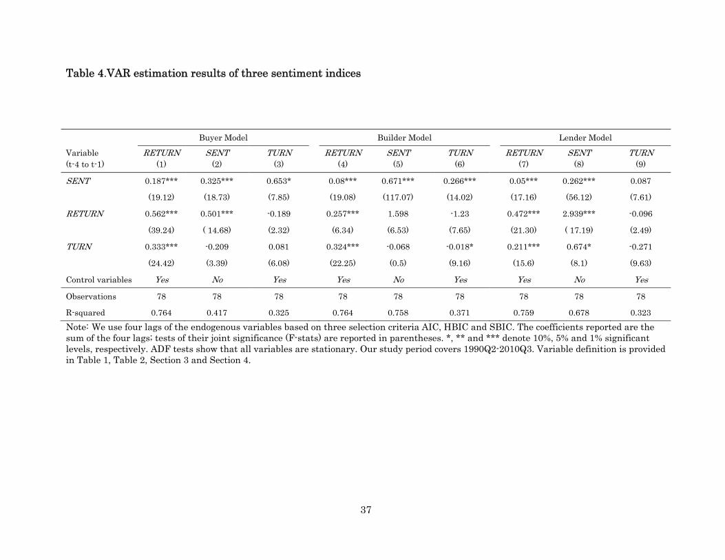
37  

Table 4.VAR estimation results of three sentiment indices

 

 

Note: We use four lags of the endogenous variables based on three selection criteria AIC, HBIC and SBIC. The coefficients reported are the sum of the four lags; tests of their joint significance (F-stats) are reported in parentheses. *, ** and *** denote 10%, 5% and 1% significant levels, respectively. ADF tests show that all variables are stationary. Our study period covers 1990Q2-2010Q3. Variable definition is provided in Table 1, Table 2, Section 3 and Section 4.            

Buyer Model Builder Model Lender Model

Variable (t-4 to t-1)

RETURN (1)

SENT (2)

TURN (3)

RETURN

(4) SENT

(5) TURN

(6)

RETURN (7)

SENT (8)

TURN (9)

SENT 0.187*** 0.325*** 0.653* 0.08*** 0.671*** 0.266*** 0.05*** 0.262*** 0.087

(19.12) (18.73) (7.85) (19.08) (117.07) (14.02) (17.16) (56.12) (7.61)

RETURN 0.562*** 0.501*** -0.189 0.257*** 1.598 -1.23 0.472*** 2.939*** -0.096

(39.24) ( 14.68) (2.32) (6.34) (6.53) (7.65) (21.30) ( 17.19) (2.49)

TURN 0.333*** -0.209 0.081 0.324*** -0.068 -0.018* 0.211*** 0.674* -0.271

(24.42) (3.39) (6.08) (22.25) (0.5) (9.16) (15.6) (8.1) (9.63)

Control variables Yes No Yes Yes No Yes Yes No Yes

Observations 78 78 78 78 78 78 78 78 78

R-squared 0.764 0.417 0.325 0.764 0.758 0.371 0.759 0.678 0.323

38  

Table 5.VAR estimation results of the composite sentiment index

                 Note: We chose four lags of endogenous variables based on three selection criteria AIC, HBIC and SBIC. The coefficients reported are the sum of four lags; tests of joint significance (F-stats) are reported in parentheses. *, ** and *** denote 10%, 5% and 1% significant levels, respectively. ADF tests show that all variables are stationary. Our study period covers 1990Q2-2010Q3. Variable definition is provided in Table 1, Table 2, Section 3 and Section 4. 

Variable (t-4 to t-1)

RETURN (1)

PCSENT (2)

TURN (3)

PCSENT 1.014*** 0.212*** 3.101***

(38.42) (65.09) (17.57)

RETURN 0.102** 0.419*** -1.54*

(9.75) (23.07) (8.11)

TURN 0.271*** -0.0332 -0.078*

(18.31) (2.69) (9.40)

Control variables Yes No Yes

Observations 78 78 78

R-squared 0.803 0.728 0.394

39  

Table 6.VAR estimation results of the composite sentiment index with FHFA housing price index                 Note: We chose two lags of endogenous variables based on three selection criteria AIC, HBIC and SBIC. The coefficients reported are the sum of two lags, and their joint significance tests (F-stats) are in parentheses. *, ** and *** denote 10%, 5% and 1% significant levels, respectively. ADF tests show that all variables are stationary. Our study period covers 1990Q2-2010Q3. Variable definition is provided in Table 1, Table 2, Section 3 and Section 4.    

Variable (t-2 to t-1)

RETURN (1)

PCSENT (2)

TURN (3)

PCSENT 0.47*** 0.76*** 1.81**

(14.77) (46.3) (7.22)

RETURN 0.22*** 0.0862 -0.896

(41.8) (2.19) (1.74)

TURN 0.02** 0.03299 -0.0721

(6.37) (2.04) (1.49)

Control variables Yes No Yes

Observations 80 80 80

R-squared 0.701 0.632 0.271

40  

Table 7. Sub-period analysis

1990Q2-1997Q4 1998Q1-2010Q3

Variable (t-4 to t-1)

RETURN (1)

PCSENT (2)

TURN (3) RETURN

(4) PCSENT

(5) TURN

(6)

PCSENT 1.17*** -0.3519 7.07*** 0.86*** 0.19*** 2.53*** 18.39 0.64 19.02 34.23 69.69 14

RETURN -0.0272 0.68** -1.935 0.014*** 0.48*** -1.291 1.1 11.42 6.81 19.05 18.47 6.28

TURN 0.02157 -0.0913 0.01*** 0.52*** -0.071 0.08*** 0.68 6.12 39.78 32.63 0.1257 13.3

Control variables Yes No Yes Yes No Yes

Observations 27 27 27 51 51 51 R-squared 0.827 0.373 0.829 0.877 0.801 0.489

Note: We chose four lags of endogenous variables based on three selection criteria AIC, HBIC and SBIC. The coefficients reported are the sum of four lags; tests of joint significance (F-stats) are reported in parentheses. *, ** and *** denote 10%, 5% and 1% significant levels, respectively. ADF tests show that all variables are stationary. The equations are estimated over 1990Q2-1997Q4 and 1998Q1-2010Q3. Variable definition is provided in Table 1, Table 2, Section 3 and Section 4.

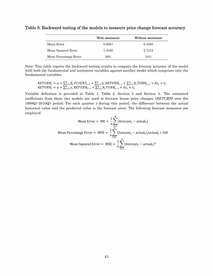
41  

Table 8. Backward testing of the models to measure price change forecast accuracy  

Note: This table reports the backward testing results to compare the forecast accuracy of the model with both the fundamental and sentiment variables against another model which comprises only the fundamental variables ∑ ∑ ∑ ∑ ∑

Variable definition is provided in Table 1, Table 2, Section 3 and Section 4.. The estimated coefficients from these two models are used to forecast house price changes (RETURN) over the 1998Q1-2010Q3 period. For each quarter t during this period, the difference between the actual historical value and the predicted value is the forecast error. The following forecast measures are employed:

MeanError ME 1n

forecast actual

MeanPercentageError MPE 1n

forecast actual /actual ∗ 100

MeanSquaredError MSE 1n

forecast actual

With sentiment Without sentiment

Mean Error 0.0087 0.1085

Mean Squared Error 1.3340 2.7512

Mean Percentage Error 28% 54%

42  

Table 9.Long-run regression results

Return horizon k Adjusted coef.

PCSENTt Bootstrapped

St. Err. R2

One-year 4 1.575*** 0.14 0.709

Two-year 8 1.100*** 0.12 0.475

Three-year 12 0.888*** 0.11 0.301

Four-year 16 0.174* 0.09 0.167

Five-year 20 -0.059 0.10 0.104

Note: The reported coefficients are bias-adjusted OLS estimates derived from the bootstrap simulation procedure documented in the Appendix B. *, ** and *** denote 10%, 5% and 1% significant levels, respectively. Variable definition is provided in Table 1, Table 2, Section 3 and Section 4.

43  

Appendix A

Bootstrap simulation procedure

We adopt the bootstrap simulation procedure described in Brown and Cliff (2005)

and Ling, Naranjo and Scheick (2013). First, the long-run regressions specified in Equation

(7) are estimated using OLS and the beta coefficients of the sentiment measure, , are

saved to calculate bias-adjusted coefficients later.

The second step involves generating a pseudo return series under the null

hypothesis that sentiment has no effect on house prices. The following VAR model is used

as the underlying data generating process of the pseudo return series:

VAR(1) for yt = [ , , ]

where is the real price changes, is our measure of sentiment, and is the

set of control variables. The beta coefficient on is set to zero to ensure that the

pseudo return series is generated under the null. The predicted y-values and residuals from

the VAR estimations are saved.

In the third step, each residual is first multiplied by {n/(n-v)}1/2 to adjust for a

downward bias that results from the use of OLS in estimating the VAR model, where n is

the number of observations and v refers to the degrees of freedom of the VAR (MacKinnon,

2002). The next step involves sampling with replacement from these residuals to generate a

new set of bootstrapped residuals. This sampling process is repeated 10,100 times but the

first 100 samples are discarded to avoid any startup effects.

Fourth, the remaining 10,000 sets of bootstrapped residuals are added to the

predicted y-value saved from the VAR estimation above to create 10,000 sets of pseudo

return series. From these pseudo return series, 10,000 new sets of k-period future returns

can be created as the dependent variables in the long-horizon model specified in Equation

(7). OLS is used to estimate the regressions with these new dependent variables, yielding

10,000 beta coefficients for each of the return horizons.

Calculating bias-adjusted beta:

The bootstrap simulation procedure discussed above can be utilized to correct for the

bias in coefficient estimates within finite sample settings when the bias function is not

44  

known analytically (see MacKinnon and Smith, 1998). Assuming the bias is constant for a

particular return horizon, the estimated bias is expressed as:

where is the OLS beta coefficient from running the original long-run regression (Step 1

above), and is the sample mean of the 10,000 simulated beta coefficients. The adjusted

beta coefficient can therefore be specified as:

2

This bias-adjusted estimator has been widely shown to provide reliable coefficient estimates

in the bootstrap literature.

Calculating adjusted t-statistics and p-values:

Since asymptotic standard errors calculated from a small sample with overlapping

observations suffer from significant downward bias, the bootstrap standard error can be

used as a more accurate alternative. It is simply the standard deviation of the 10,000

simulated beta coefficients:

∑

where is the estimated beta coefficient from iteration i of the simulation process, is the

sample mean of the 10,000 simulated coefficients, and B is the number of simulations. The

new bias-adjusted t-statistic can be calculated as follows:

Because the t-statistics constructed in this manner do not always follow the

standard t-distribution, we develop a bootstrap distribution of t-statistics to compute more

accurate p-values for testing of the null hypothesis. The bootstrap t-distribution is derived

from 10,000 adjusted t-statistics of the simulation process:

∗

where is the estimated beta coefficient from iteration i of the simulation process, is the

sample mean of the 10,000 simulated betas, and is the bootstrap standard error. This

technique generates an empirical distribution of the t-statistics that provides new critical

values for hypothesis testing.

45  

Finally, assuming the distribution is symmetric around zero, p-values can be

calculated as:

∑ | ∗|

where ∙ denotes the indicator function, which equals 1 if its argument is true and 0

otherwise, | ∗|is the absolute value of the t-statistic of iteration i, is the absolute

value of the bias-adjusted t-statistic, and B is the number of simulations.