Experiments withExperiments withMonthly Monthly Satellite Ocean Color FieldsSatellite Ocean Color Fields

in a NCEP Operational Ocean Forecast Systemin a NCEP Operational Ocean Forecast System

PI: Eric Bayler, NESDIS/STARPI: Eric Bayler, NESDIS/STAR

Co-I: David Behringer, NWS/NCEP/EMC/GCWMBCo-I: David Behringer, NWS/NCEP/EMC/GCWMB

Co-I: Avichal Mehra, NWS/NCEP/EMC/MMABCo-I: Avichal Mehra, NWS/NCEP/EMC/MMAB

Sudhir Nadiga, NWS/NCEP/EMC – IMSGSudhir Nadiga, NWS/NCEP/EMC – IMSG

BackgroundBackground

Penetration and absorption of solar insolation in the upper layers of the ocean is affected by the optical properties of the water column

The vertical distribution of heating due to the absorption of solar radiation affects near-surface heat content and vertical stability

• Affects surface heat flux

Chlorophyll concentration has been found to correlate to the optical properties of water column

NCEP operational models employ a limited climatology (1998-2001) of satellite (SeaWiFS) ocean color data for modeling this process

2

SeaWiFS

MotivationMotivation

Improved ocean and coupled ocean-atmosphere forecasts

Better representation of vertical distribution of solar radiation over the water column by properly representing temporal changes

Reduce biases and need for constraining the model (relaxation to observed surface and subsurface fields)

Transition towards operational near-real-time use of VIIRS ocean color data in operational ocean modeling

3

NPP/JPSS VIIRS

NCEP OPERATIONAL OCEAN NCEP OPERATIONAL OCEAN MODEL MODEL

NOAA/OAR/GFDL Modular Ocean Model (MOM4) Global Ocean Data Assimilation System (GODAS) / Coupled

Forecast System (CFS) Grid:

Tripolar 1/2°×1/2° equatorial region: 1/2°×1/4°

Relaxation: SST – 30-day to daily Reynolds ¼-degree optimally interpolated SST SSS – 30-day to WOA 2009 SSS annual mean

Reference: Behringer, D. W., The Global Ocean Data Assimilation System at NCEP, AMS 87th

Annual Meeting, 2007.

4

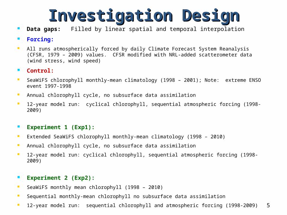
InvestigationInvestigation Design Design Data gaps: Filled by linear spatial and temporal interpolation

Forcing: All runs atmospherically forced by daily Climate Forecast System Reanalysis (CFSR,

1979 – 2009) values. CFSR modified with NRL-added scatterometer data (wind stress, wind speed)

Control: SeaWiFS chlorophyll monthly-mean climatology (1998 – 2001); Note: extreme ENSO

event 1997-1998

Annual chlorophyll cycle, no subsurface data assimilation

12-year model run: cyclical chlorophyll, sequential atmospheric forcing (1998-2009)

Experiment 1 (Exp1): Extended SeaWiFS chlorophyll monthly-mean climatology (1998 – 2010)

Annual chlorophyll cycle, no subsurface data assimilation

12-year model run: cyclical chlorophyll, sequential atmospheric forcing (1998-2009)

Experiment 2 (Exp2): SeaWiFS monthly mean chlorophyll (1998 – 2010)

Sequential monthly-mean chlorophyll no subsurface data assimilation

12-year model run: sequential chlorophyll and atmospheric forcing (1998-2009)5

Environmental State ReferenceEnvironmental State Reference

Climate Forecast System Reanalysis (CFSR) Reanalysis defines the mean states of the atmosphere, ocean, land surface and

sea ice Global, high-resolution, coupled atmosphere-ocean-land surface-sea ice model

system provides the best estimate of the state of these coupled domains over the period 1979 – 2009

Continually assimilated the best possible observation data Hourly time resolution and 0.5° horizontal resolution

Produced using the MOM model, the same model used for the control and experiment cases

Employs control case chlorophyll climatology; however, the reanalysis continually assimilates the best available observations (vertical profiles of temperature, salinity, satellite altimeter data, etc.), largely correcting for the influences of chlorophyll

Saha, S., et al., 2010, “The NCEP Climate Forecast System Reanalysis,” Bull. Amer. Meteor. Soc., 91, 1015-1057.

CFSR atmosphere forcing used for the control case and both experiments

Results referenced to CFSR ocean state values

6

Analysis DefinitionsAnalysis Definitions Anomaly:

Difference from designated reference (specified monthly-mean annual cycle) Index (i) represents month of data record, e.g. (i = 1) = Jan 1998

Root Mean Square Error (RMSE) RMSE includes:

Differences in monthly-mean annual cycles Differences in anomalies

Index (i) represents month of data record; e.g. (i = 1) = Jan 1998

Normalized RMSE difference RMSE comparison of specified cases with respect to a common reference Expressed in terms of percentage of the Control’s RMSE with respect to the common

reference

7

Control Case: Limited Ocean Color Climatology

Upper-ocean temperature variability

Pacific “Cold Tongue”(2S – 2N, 120W)

Temperature (C)

8

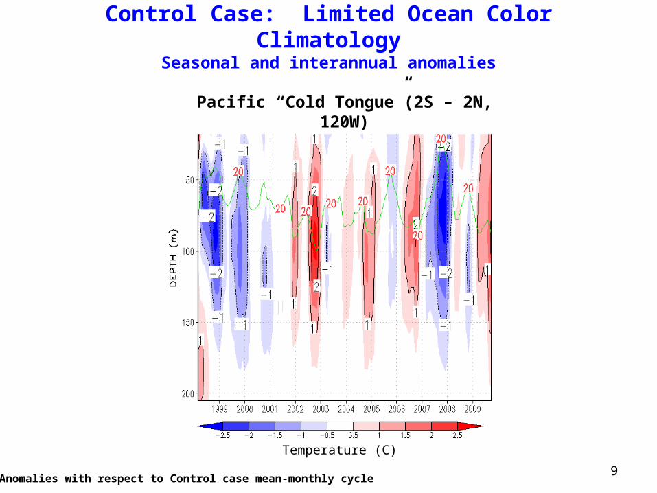
Control Case: Limited Ocean Color Climatology

Seasonal and interannual anomalies

Temperature (C)

* Anomalies with respect to Control case mean-monthly cycle 9

Pacific “Cold Tongue”(2S – 2N, 120W)

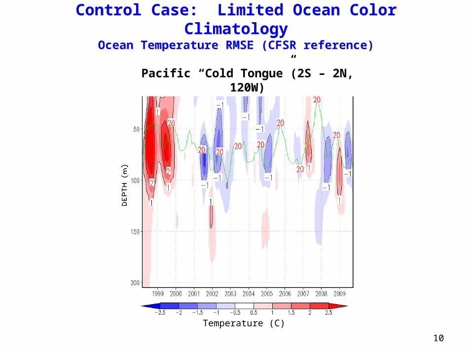
Control Case: Limited Ocean Color Climatology

Ocean Temperature RMSE (CFSR reference)

Temperature (C)

10

Pacific “Cold Tongue”(2S – 2N, 120W)

Exp2: Sequential Monthly-mean Ocean ColorOcean Temperature RMSE (CFSR reference)

Temperature (C)

11

Pacific “Cold Tongue”(2S – 2N, 120W)

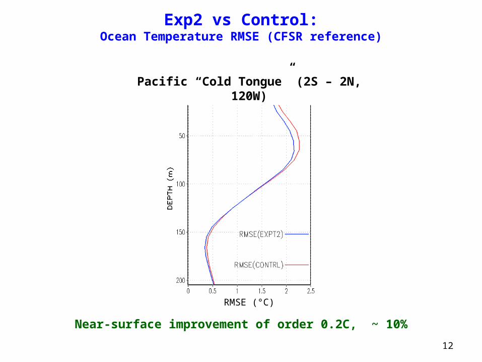
Exp2 vs Control:Ocean Temperature RMSE (CFSR reference)

Pacific “Cold Tongue” (2S – 2N, 120W)

RMSE (°C)

Near-surface improvement of order 0.2C, ~ 10%

12

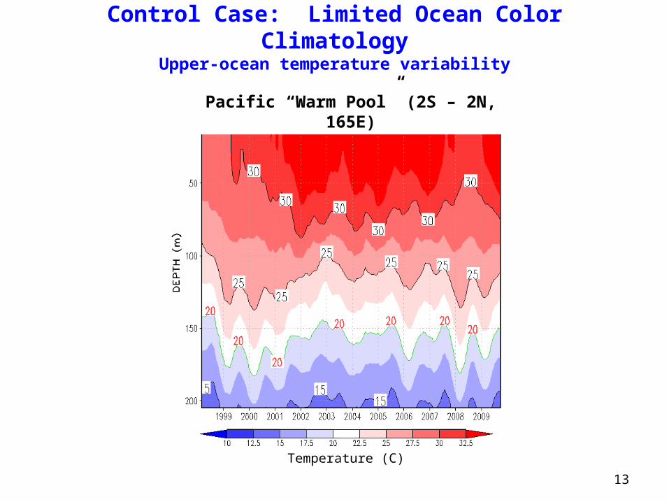
Control Case: Limited Ocean Color Climatology

Upper-ocean temperature variability

Temperature (C)

13

Pacific “Warm Pool” (2S – 2N, 165E)

Temperature (C)

Control Case: Limited Ocean Color Climatology

Seasonal and interannual anomalies

14

Pacific “Warm Pool” (2S – 2N, 165E)

15

Temperature (C)

Control Case: Limited Ocean Color Climatology

Ocean Temperature RMSE (CFSR reference)

Pacific “Warm Pool” (2S – 2N, 165E)

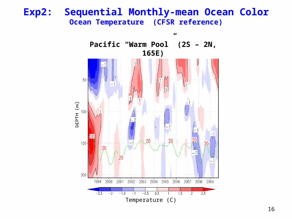
16

Temperature (C)

Exp2: Sequential Monthly-mean Ocean ColorOcean Temperature (CFSR reference)

Pacific “Warm Pool” (2S – 2N, 165E)

17

Exp2 vs Control:Ocean Temperature RMSE (CFSR reference)

Pacific “Warm Pool” (2S – 2N, 165E)

RMSE (°C)

Minor near-surface improvement

18

Near-surface Temperature RMSEControl Case (CFSR reference)

Equatorial Zonal Cross-section (2S – 2N)

Temperature (C)

19

Near-surface Temperature RMSEExp1 (CFSR reference)

Equatorial Zonal Cross-section (2S – 2N)

Temperature (C)

20

Temperature (C)

Equatorial Zonal Cross-section (2S – 2N)

Near-surface Temperature RMSEExp2 (CFSR reference)

21

Equatorial Zonal Cross-section (2S – 2N)

Temperature (C)

Near-surface Temperature RMSEExp1 – Control: Impact magnitude of extended ocean color

climatology

0.05

22

Equatorial Zonal Cross-section (2S – 2N)

Temperature (C)

Near-surface Temperature RMSEExp2 – Exp1: Additional impact magnitude from sequential ocean

color data

0.05

23

Equatorial Zonal Cross-section (2S – 2N)

Temperature (C)

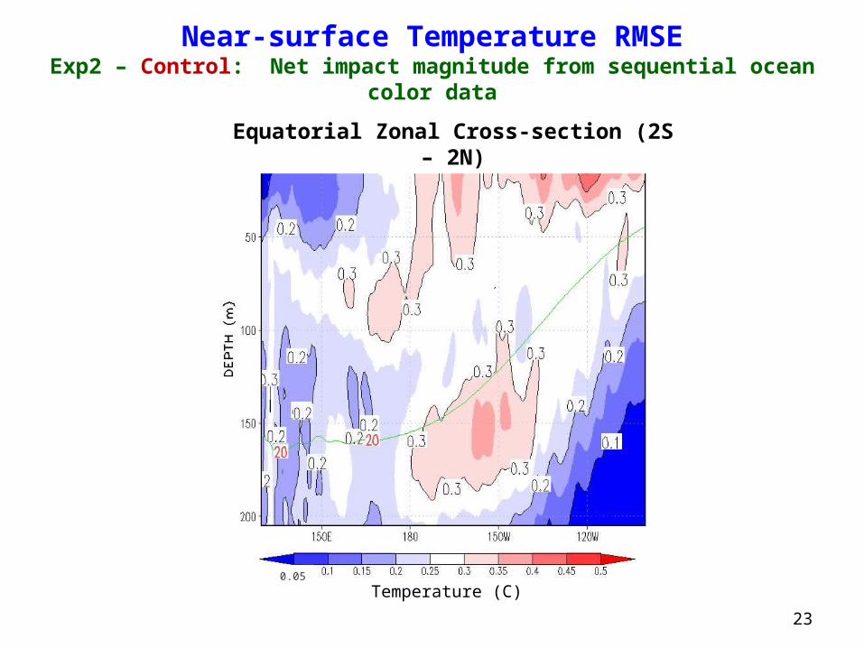
Near-surface Temperature RMSEExp2 – Control: Net impact magnitude from sequential ocean

color data

0.05

24

Equatorial Zonal Cross-section (2S – 2N)

Temperature (C)

Near-surface Temperature RMSE Differences:Extended Ocean Color Climatology

RMSE (Exp1) – RMSE (Control): CFSR reference

25

Equatorial Zonal Cross-section (2S – 2N)

Temperature (C)

Near-surface Temperature RMSE Differences:Sequential Ocean Color Data

RMSE (Exp2) – RMSE (Exp1): CFSR reference

26

Equatorial Zonal Cross-section (2S – 2N)

Temperature (C)

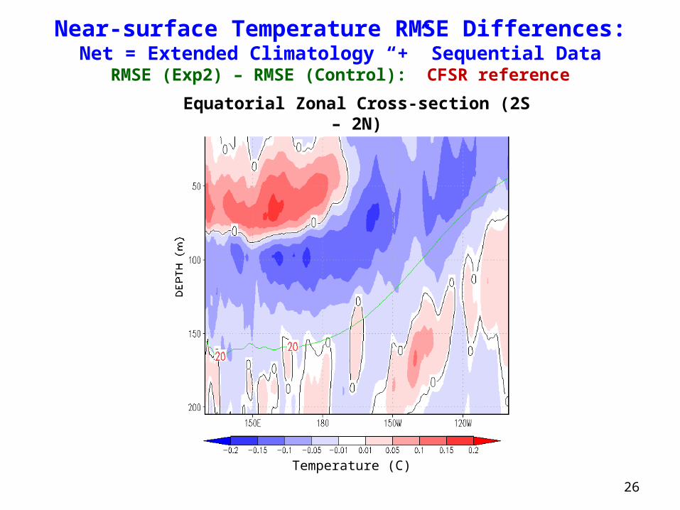
Near-surface Temperature RMSE Differences:Net = Extended Climatology “+” Sequential Data

RMSE (Exp2) – RMSE (Control): CFSR reference

27

Equatorial Zonal Cross-section (2S – 2N)

Percent

Normalized Near-surface Temperature RMSE Differences Extended Ocean Color Climatology

28

Equatorial Zonal Cross-section (2S – 2N)

Percent

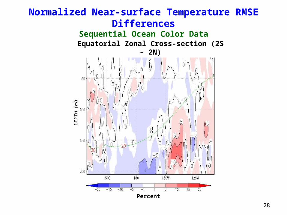
Normalized Near-surface Temperature RMSE Differences

Sequential Ocean Color Data

29

Equatorial Zonal Cross-section (2S – 2N)

Percent

Normalized Near-surface Temperature RMSE Differences

Net = Extended Climatology “+” Sequential Data

32

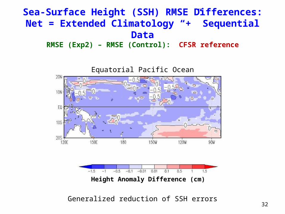
Height Anomaly Difference (cm)

Equatorial Pacific Ocean

Sea-Surface Height (SSH) RMSE Differences:Net = Extended Climatology “+” Sequential

DataRMSE (Exp2) – RMSE (Control): CFSR reference

Generalized reduction of SSH errors

35

Equatorial Pacific Ocean

Percent

Normalized Sea-Surface Height (SSH) RMSE Differences:

Net = Extended Climatology “+” Sequential DataRMSE (Exp2) – RMSE (Control): CFSR reference

Generalized reduction of SSH errors

38

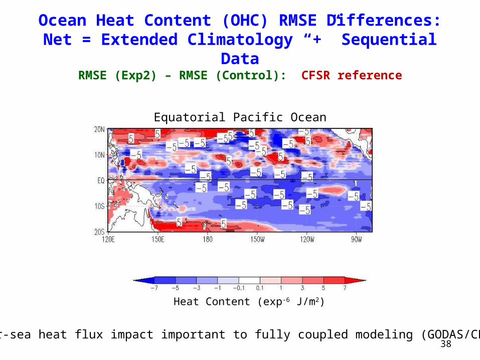
Equatorial Pacific Ocean

Heat Content (exp-6 J/m2)

Ocean Heat Content (OHC) RMSE Differences:Net = Extended Climatology “+” Sequential

DataRMSE (Exp2) – RMSE (Control): CFSR reference

Air-sea heat flux impact important to fully coupled modeling (GODAS/CFS)

41

Equatorial Pacific Ocean

Percent

Normalized Ocean Heat Content (OHC) RMSE Differences:

Net = Extended Climatology “+” Sequential DataRMSE (Exp2) – RMSE (Control): CFSR reference

Air-sea heat flux impact important to fully coupled modeling (GODAS/CFS)

SummarySummary Chlorophyll:

Simulations with monthly SeaWiFS ocean chlorophyll data reduce subsurface temperature errors. Most changes in temperature are found just above the seasonal thermocline (20C isotherm)

Sea-Surface Height (SSH): Reductions of SSH errors in the equatorial cold tongue region and north of the

equator are in the 5-10% range

Ocean Heat Content (OHC): Reductions of ocean heat content errors south of the equator and in the cold tongue

region are in the 1-10% range

Currently constrained at surface. When fully coupled (GODAS/CFS), differences will influence air-sea heat fluxes.

NEXT: Comparisons of model output with real data for validation; (in situ vertical profiles of

temperature, salinity, velocity) from Pacific/Atlantic/Indian Ocean arrays and satellite altimetry

Near-real-time ocean color assimilation

Extend study to assess ocean color assimilation impact on the operational results for NOAA’s Real-Time Ocean Forecast System (RTOFS), based on the HYCOM model

Unify NOAA’s ocean color data assimilation methodology for the operational models (GODAS, RTOFS)

42