Louisiana State UniversityLSU Digital Commons

LSU Master's Theses Graduate School

2017

Experimental Study of Frequency Oscillations inIslanded Power SystemKevin Daniel WellmanLouisiana State University and Agricultural and Mechanical College, kwellm1@lsu.edu

Follow this and additional works at: https://digitalcommons.lsu.edu/gradschool_theses

Part of the Electrical and Computer Engineering Commons

This Thesis is brought to you for free and open access by the Graduate School at LSU Digital Commons. It has been accepted for inclusion in LSUMaster's Theses by an authorized graduate school editor of LSU Digital Commons. For more information, please contact gradetd@lsu.edu.

Recommended CitationWellman, Kevin Daniel, "Experimental Study of Frequency Oscillations in Islanded Power System" (2017). LSU Master's Theses. 4590.https://digitalcommons.lsu.edu/gradschool_theses/4590

EXPERIMENTAL STUDY OF FREQUENCY OSCILLATION IN ISLANDED POWER SYSTEM

A Thesis

Submitted to the Graduate Faculty of the Louisiana State University and

Agricultural and Mechanical College in partial fulfilment of the

requirements for the degree of Master of Science in Electrical Engineering

in

The Department of Electrical and Computer Engineering

by Kevin Daniel Wellman

B.S., Mississippi State University, 2011 August 2017

ii

ACKNOWLEDGEMENTS

I would like to thank Louisiana State University and Entergy Corporation for funding this

project. I would also like to thank Dr. Shahab Mahraeen for teaching and the wealth of

information he gave to me. I would also like to thank Pooria Mohammadi and other students

for the assistance while working on the experiments.

iii

TABLE OF CONTENTS

ACKNOWLEDGEMENTS……………………………………………………………………….……………………………..………ii

ABSTRACT………………………………………………………………………………………..…….………..………………….…...iv

1. INTRODUCTION ……………………………………………………………………………………………………..……………1

1.1. Introduction………………………………………………………………………………………………………………….1

2. THEORETICAL BACKGROUND……………………………………………………………………………………………….4

2.1. Transient Stability………………………………………………………………………………………………………….4

2.2. Generator Model……………………………………….………………………………………………………………….7

2.3. Design of PSS ……………………………………………………………………………………………………………….9

3. POWER SYSTEM DESIGN………………………………………………………………………………………………….…13

3.1. Motor Generator Set…………...………………………………..………………………………………….……….13 3.2. Inertia Calculation………………..……………………………………………………………………….…………….15 3.3. Control Mechanism………………………………………………………………………………………………….…16 3.4. Power System Stabilizer……………..……………………………………………………………………….………21 3.5. Transmission Lines and Loads……………………………………………………………………………………..23 3.6. Photo Voltaic Cells….…………………………………………………………………………………………………..24

4. EXPERIMENTS…………………………………………………………………………………………………………………….25

4.1. Simulation Model…………….………………………………………………………………………………………...25 4.2. Physical Model………………………………………………………………………………………….…………..……30 4.3. Conclusion……………………………………………………………………………………………….……………..….34

5. SUMMARY…………………………………………………………………………………………………………..……………35

REFERENCES………………………………………………………………………………………………………….………………..36

APPENDIX: IEEE 14 BUS…………………………..…………………………………………………………….………………..37

VITA…………………………………………………………………………………………………………………………………….….41

iv

ABSTRACT

Since the introduction of power electronics to the grid, the power system has quickly

changed. Fault detection and removal is performed more accurately and at quicker response

time, and non-inertia driven loads have been added. This means stability must continue to be a

main topic of concern to maintain a stable synchronized grid.

In this thesis a lab was designed, constructed, and tested for the purpose of studying

transient stability in power systems. Many different options were considered and researched,

but the focus of this paper is to describe the options chosen. The lab must be safe to operate

and work around, have flexibility to perform many different type of experiments, and

accurately simulate a power system.

The created lab was then tested to observe the impact of PSS on an unsynchronized

generator connected to a static load. The lab performed as designed, which allows for the

introduction of more machines to create the IEEE 14 Bus grid.

1

CHAPTER 1: INTRODUCTION

1.1 Introduction

The first power grid was built in England in 1881, with numerous patents created in the

following years. Thomas Edison insisted on a Direct Current system, but this proved to be

inefficient due to high line loss at low voltage levels. It was not until the 1930’s when power

electronics were created to simplify voltage transformations on DC systems. Instead, the grid

was designed for Alternating Current by utilizing Nikola Telsa’s patents on transformers and

induction motors. The world electrical demand has grown to nearly 23,000 TWh/year according

to the International Energy Agency. Electricity not only provides comfort and entertainment,

but more importantly, sustaining life.

Stability, a system’s ability to return to equilibrium after a disturbance, is a key

component necessary for reliable operation of any system. In the 1920’s, damping was solved

by introducing generator damper windings and changing prime mover design to turbine style.

Since the introduction of power electronics, the grid has quickly evolved and become more

complicated. Modern systems contain non-inertia driven equipment and components incapably

of supplying reactive power. The response time to an event must be decreased to maintain

stable operation. Generator stability can be broken down into three main categories: steady-

state, transient, and dynamic.

Steady state instabilities occurs in the time periods of 0 to 10−3 seconds. These include

lightning and switching surges and stator transients and sub-synchronous resonance. Due to

2

Figure 1.1: Power System Instability

the high response time required, passive components such as Metal-Oxide Varistor arrestors or

capacitors are utilized. These components chop waveform peaks and smooth out the

corresponding oscillations.

Transient stability occurs in the time period of sub-seconds to tens of seconds. These

disturbances are caused by fluctuation in load or generation. A synchronous power system

must operate at equilibrium, meaning generation must always equal consumption.

Consumption includes energy used to drive rotating equipment, line losses, and faults. When

load is added, frequency decreases and inertia of the generator supplies the additional load.

Additional energy must be then supplied to the prime mover to keep the system in equilibrium.

The dampening of these oscillation generally occurs by synchronous machine dynamics or

3

power electronics component compensation. Systems such as a Power System Stabilizer can

increase the damping ability of a generator.

Dynamic stability is a slow response requiring tens of seconds to minutes of time. These

stabilizers are used to control load fluctuations by reducing energy created by the generator

prime mover. Examples would include adjusting fuel delivered to boiler for steam driven

equipment, regulating fuel delivery to combustion driven generators, or modifying the pitch of

wind powered generators.

System studies can be performed by using advanced software, but at times, a physical

model may need to be created in order to validate the results. The LSU Generator Stability Lab

was designed to handle a variety of experiments. These experiments may be performed

synchronized to the grid or isochronous. Photovoltaic cells and inverters are included in the lab

to be able to model a micro grid or grid containing only non-inertia driven power sources. A key

component of a university is creating a learning environment for faculty and student. The lab

creates unique opportunity for fostering education through use of a small scale power system.

Topics can be focused on stability, fault analysis, protection systems, PV integration, harmonics,

or motor dynamics.

This paper description the purpose for the lab, selection of components, integration of

system, and frequency oscillations in an islanded system. Many different options were

evaluated, but the focus of this paper is to discuss the designed system.

4

CHAPTER 2: THEORETICAL BACKGROUND

2.1 Transient Stability

Although the power system may be considered a robust system of networks connected

over thousands of miles, oscillations are continuously observed. These can be presented as

frequency or voltage related. Elimination of the initiator is viewed as unrealistic, since it may be

in the form of lightning impulses, load oscillations, or faults. Transients in the power system are

caused by large disturbances, such as faults, loss of generation, or sudden load changes. The

power angle is used to determine whether the machine can return to steady-state operation

after a transient occurs.

The rotor motion is defined by Newton’s second law.

𝐽𝑑2𝜃

𝑑𝑡2 = 𝑇𝑚 − 𝑇𝑒 = 𝑇𝛼 (2.1)

Where

J = total moment of inertia of the rotating mass, 𝑘𝑔𝑚2

Θ = angular position of the rotor in rad

𝑇𝑚 = 𝑚𝑒𝑐ℎ𝑎𝑛𝑖𝑐𝑎𝑙 𝑡𝑜𝑟𝑞𝑢𝑒 𝑠𝑢𝑝𝑝𝑙𝑖𝑒𝑑 𝑏𝑦 𝑡ℎ𝑒 𝑝𝑟𝑖𝑚𝑒 𝑚𝑜𝑣𝑒𝑟 𝑚𝑖𝑛𝑢𝑠

𝑡ℎ𝑒 𝑟𝑒𝑡𝑎𝑟𝑑𝑖𝑛𝑔 𝑡𝑜𝑟𝑞𝑢𝑒 𝑑𝑢𝑒 𝑡𝑜 𝑚𝑒𝑐ℎ𝑎𝑛𝑖𝑐𝑎𝑙 𝑙𝑜𝑠𝑠, 𝑁𝑚

𝑇𝑒 = 𝑒𝑙𝑒𝑐𝑡𝑟𝑖𝑐𝑎𝑙 𝑡𝑜𝑟𝑞𝑢𝑒 𝑡ℎ𝑎𝑡 𝑎𝑐𝑐𝑜𝑢𝑛𝑡𝑠 𝑓𝑜𝑟 𝑡ℎ𝑒 𝑡𝑜𝑡𝑎𝑙 𝑡ℎ𝑟𝑒𝑒 𝑝ℎ𝑎𝑠𝑒 𝑒𝑙𝑒𝑐𝑡𝑟𝑖𝑐𝑎𝑙 𝑝𝑜𝑤𝑒𝑟 𝑜𝑢𝑡𝑝𝑢𝑡

𝑜𝑓 𝑡ℎ𝑒 𝑔𝑒𝑛𝑒𝑟𝑎𝑡𝑜𝑟, 𝑝𝑙𝑢𝑠 𝑒𝑙𝑒𝑐𝑡𝑟𝑖𝑐𝑎𝑙 𝑙𝑜𝑠𝑠, 𝑁𝑚

𝑇𝑎 = 𝑁𝑒𝑡 𝑎𝑐𝑐𝑒𝑙𝑒𝑟𝑎𝑡𝑖𝑛𝑔 𝑡𝑜𝑟𝑞𝑢𝑒, 𝑁𝑚

Inertia constant is then normalized to:

5

𝐻 =𝑆𝑡𝑜𝑟𝑒𝑑 𝐾𝑖𝑛𝑒𝑡𝑖𝑐 𝐸𝑛𝑒𝑟𝑔𝑦 𝑎𝑡 𝑆𝑦𝑛𝑐ℎ𝑟𝑜𝑛𝑜𝑢𝑠 𝑆𝑝𝑒𝑒𝑑(𝑀𝑒𝑔𝑎 𝐽𝑜𝑢𝑙𝑒𝑠)

𝐺𝑒𝑛𝑒𝑟𝑎𝑡𝑜𝑟 𝑀𝑉𝐴 𝑅𝑎𝑡𝑖𝑛𝑔=

𝐽 𝜔22

2𝑆𝑅𝑎𝑡𝑒𝑑 (2.2)

Per unit swing equation is defined as the following:

2𝐻

𝜔𝑠 (𝑑2𝛿(𝑡)

𝑑𝑡2) = 𝑃𝑚(𝑡) − 𝑃𝑒(𝑡) = 𝑃𝑎(𝑡) (2.3)

Where 𝛿 = 𝑝𝑜𝑤𝑒𝑟 𝑎𝑛𝑔𝑙𝑒

Swing equation can then be converted to two 1st order derivatives.

dΔ𝜔𝑟

dt=

2

2𝐻(𝑃𝑚 − 𝑃𝑒) (2.4)

dδ

dt= 𝜔𝑠𝑚𝑥Δω𝑟) (2.5)

The power angle is the angle between the generator internal and terminal voltage

phasor. Every machine has a critical angle in which if this angle is surpassed, then the machine

can never return to a steady state. The equal area criterion is used to describe a machine’s

response to transients. Equal Area Criterion is broken down into three distinct time periods:

𝐴1 𝑖s pre-fault, 𝐴2 is during the fault, and 𝐴3is post-fault. When areas under the curve are

equal, the machine is in equilibrium and stable.

6

Figure 2.1: Equal Area Criterion Chart

𝐴1 = ∫ (𝑃𝑚 − 𝑃𝑒𝑓𝛿𝑐𝑙

𝛿0sin (𝛿)) 𝑑𝛿 (2.6)

=∫ µ 𝑑𝜔

𝑑𝑡

𝑡𝑐𝑙

𝑡0𝑥 𝜔 𝑑𝑡

=1

2µ 𝜔𝑐𝑙

2 = 𝐾𝑖𝑛𝑒𝑡𝑖𝑐 𝐸𝑛𝑒𝑟𝑔𝑦

𝐴2 = ∫ (𝑃𝑒 𝑝𝑓 sin(𝛿) − 𝑃𝑚𝛿𝑢

𝛿𝑐𝑙) 𝑑𝛿 (2.7)

=∫ µ 𝑑𝜔

𝑑𝑡

𝛿𝑢

𝛿𝑐𝑙 𝑑𝛿

= −[1

2µ 𝜔𝑢

2 −1

2µ 𝜔𝑐𝑙

2 ]

= 𝑃𝑜𝑡𝑒𝑛𝑡𝑖𝑎𝑙 𝐸𝑛𝑒𝑟𝑔𝑦 = 𝐸𝑛𝑒𝑟𝑔𝑦 𝑡𝑜 𝑏𝑒 𝐴𝑏𝑠𝑜𝑟𝑏𝑒𝑑 𝑏𝑦 𝑡ℎ𝑒 𝑆𝑦𝑠𝑡𝑒𝑚

𝐴3 = ∫ (𝑃𝑒 𝐸𝐸 sin(𝛿) − 𝑃𝑚𝛿𝑐𝑙

𝛿𝑑) 𝑑𝛿 (2.8)

=∫ µ 𝑑𝜔

𝑑𝑡

𝛿𝑐𝑙

𝛿𝑑 𝑑𝛿

7

= −[1

2µ 𝜔𝑐𝑙

2 −1

2µ 𝜔𝑑

2]

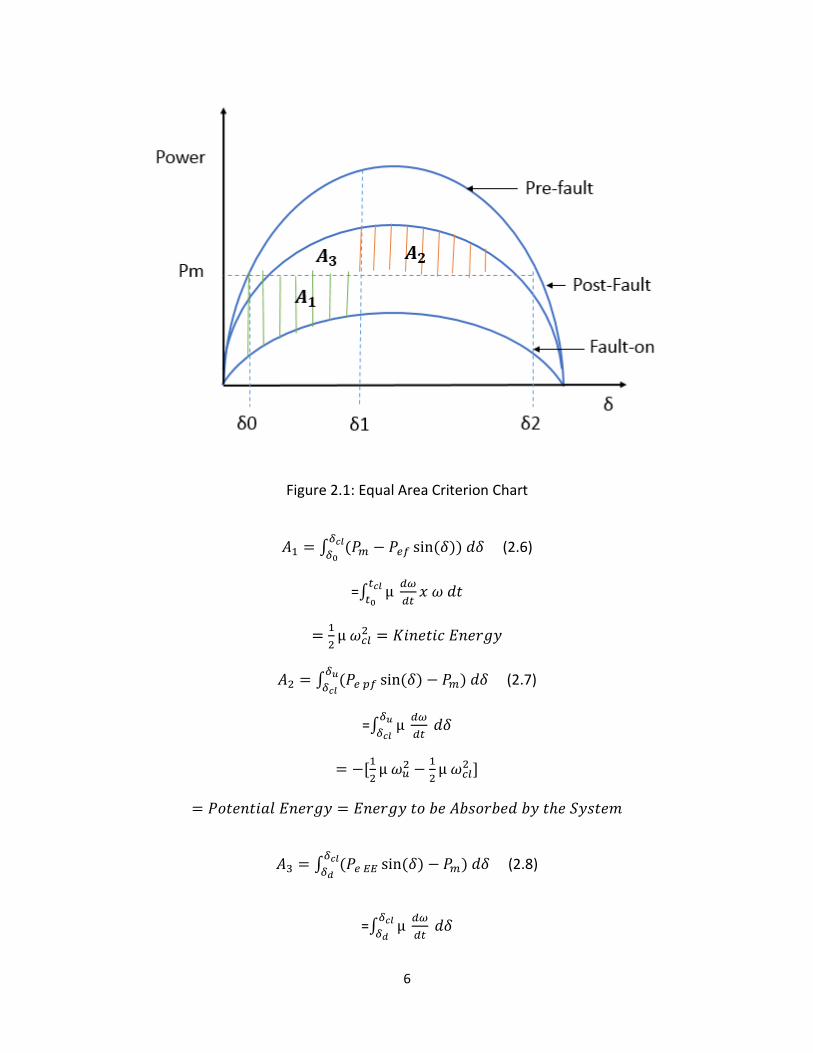
Transient Energy Function is now defined as:

𝑉(𝛿, 𝜔) =1

2𝑀𝜔2 − 𝑃𝑚(𝛿 − 𝛿𝑠) − 𝑃𝑒 𝑃𝐹 (cos 𝛿 − cos 𝛿𝑠) (2.9)

Then

𝐴2 + 𝐴3 = 𝑉(𝛿𝑢, 0) = 𝐴1 + 𝐴3 = 𝑉(𝛿𝑐𝑙, 𝜔𝑐𝑙) (2.10)

2.2 Generator Model

Synchronous generator dynamic models are used to confirm system stability and predict

post fault quantities. For this paper, three different models will be discussed. The higher

complexity leads to more precise modeling, and the one axis model is used for PSS control.

Classical model is the least complex of all, and is sufficient for analyzing swing stability.

The classical model consists of a constant voltage source and subtransient reactance. This

model is best utilized when observing response to an event on an infinite bus.

One axis model includes the d axis, whereas the two axis model adds the d and q axis.

For a rotating field to exist, there must be a three phase voltage present in the stator windings,

and the stator windings are considered to be sinusoidally distributed. D axis is in the direction

of the rotor DC magnetic field, and q axis is perpendicular. Q axis includes damper windings

known as ammortisseur. Inductances and reluctances between the axis’ are completely

separate.

8

Figure 2.2: Synchronous Machine dq Axis Diagram

One axis model is created by utilizing the equivalent circuit in Figure 2.3. From there,

algebraic equations are converted to form dynamic equations. Generator datasheets contain

necessary information to obtain machine resistances and reactances.

Figure 2.3: One Axis Equivalent Circuit

⋵ ′𝑞 = −1

𝑇′𝑑0

(𝐸′𝑞 + (𝑋𝑑 − 𝑋′

𝑑)𝐼𝑑 − 𝐸𝑓𝑑 (2.11)

�̇� = 𝜔 − 𝜔𝑠 (2.12)

9

�̇� =𝜔𝑠

2𝐻(𝑃𝑚 − (𝐸′

𝑞𝐼𝑞 + (𝑋𝑞 − 𝑋′𝑑)𝐼𝑑𝐼𝑞 (2.13)

0 = 𝑅𝑠𝐼𝑑 − 𝑋𝑞𝐼𝑞 + 𝑉𝑑 (2.14)

0 = 𝑅𝑠𝐼𝑞 + 𝑋′𝑑𝐼𝑑 + 𝑉𝑞 − 𝐸′𝑞 (2.15)

0 = 𝑅𝑒𝐼𝑑 − 𝑋𝑒𝐼𝑞 − 𝑉𝑑 + 𝑉∞𝑠𝑖𝑛𝛿 (2.16)

0 = 𝑅𝑒𝐼𝑞 + 𝑋𝑒𝐼𝑑 − 𝑉𝑞 + 𝑉∞𝑐𝑜𝑠𝛿 (2.17)

Model can then be linearized to form equation 2.18. Damping of oscillations occur by

controlling inputs, 𝑃𝑚𝑖 and 𝑉𝑟𝑒𝑓.

0 = [𝐴1]

[ 𝛥𝐸′

𝑞𝑖

𝛥𝛿𝑖

𝛥𝜔𝑖

𝛥𝐸𝑓𝑑𝑖]

+ [𝐵11 ⋮ 𝐵21] [𝛥𝑦′

𝑖

𝛥𝑦′′𝑖

] + 𝐶11 [𝛥𝑃𝑚𝑖

𝛥𝑉𝑟𝑒𝑓] (2.18)

2.3 Design of PSS

Since oscillations are present on most systems, dampeners must be designed and

installed to reduce the impact. When dampeners are inadequate, the oscillations will increase

until the system is unstable and unable to resolve itself.

Oscillations in power systems may be caused by the generator and prime mover or by

an outside source. Rotor dynamics and turbine load swings are examples of oscillations caused

by the machine. Whereas other machines on the power systems, electrical fault, or load

changes can produce these disturbances. Fast response to disturbances greatly improves the

reliability of the systems.

10

A turbine driven generator has several different methods to dampen oscillations. A

Power System Stabilizer (PSS) utilizes the voltage regulator to dampen electromechanical

oscillations. PSS manipulates the electric torque to stabilize the shaft speed and return it to a

stable system. PSS utilizes 2 key quantities: shaft speed and electrical power.

11

Figure 2.4: IEEE AVR Block Diagram [3]

12

Figure 2.5: Simulink AVR Exciter Block Diagram

The exciter is represented by the following transfer function between the exciter

voltage, Vfd and the regulator's output, ef.

𝑉𝑓𝑑

𝑒𝑓=

1

Ke+sTe (2.19)

13

CHAPTER 3: POWER SYSTEM DESIGN

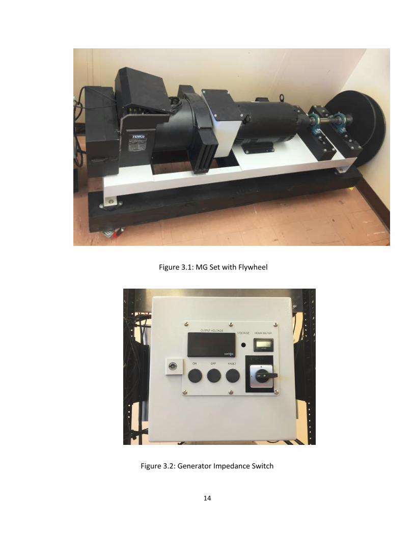
3.1 Motor Generator Set

The LSU Generator Stability Lab was designed to handle a variety of experiments

including generator stability, PV system integration, and micro-grid design. The main

components of this lab are the generator, prime mover, loads, and respective control systems.

Motor generator (MG) set was specified and purchased for the lab. The main constraint was to

operate at a lower speed and voltage for safety reasons, but also a high enough level to

properly perform experiments. The lab operates at 240V 3 phase 60Hz and the MG set is

rotating at 1800 rpm. The system was designed to be mobile, by adding casters to all

equipment, to allow more flexible for future experiments.

The generator is a brushless synchronous machine directly coupled to an induction

motor, which serves as the prime mover. The generator and motor are 4 pole air cooled

machines rated for 7.2kVA. The Non Drive End of the generator houses an incremental encoder

for speed reference. Encoder utilizes 3 channels at 360 pulses per revolution which allows

precise speed measurement, but also rotor position within 45ᵒ.

Generator impedance switch was created to change the impedance of the generator.

This allow the machine to operate in parallel impedance wye or single impedance wye. Thermal

magnetic breaker are included to ensure generator is not damaged during operation.

14

Figure 3.1: MG Set with Flywheel

Figure 3.2: Generator Impedance Switch

15

3.2 Inertia Calculation

Industrial steam turbines and gas turbines have a high inertia value due to the rotating

mass and high speed operation. This help to dampen oscillations and continue to provide

power during transient events. Flywheels were needed to increase the inertia of the motor

generator set to better simulate a steam or gas turbine operation. Two flywheels were

designed and manufactured. Thus, the flywheels were specified with an H =1 and H = 5. Listed

below are the formulas used to provide the specification of the flywheels.

𝐻 = 0.5 𝐽 (𝜔𝑏 ×2

𝜋)2/𝑆𝑏 (3.1)

𝐽 = (M × 𝑟2)/2 (3.2)

𝑉𝑜𝑙𝑢𝑚𝑒 = π × 𝑟2 × ℎ (3.3)

Table 3.1: Motor and Generator Inertia at Synchronous Speed (1800 rpm)

Generator H 0.052 kg 𝑚2

Motor H 0.040 kg 𝑚2

Lab requirement mandated the flywheels to be easily changeable, so weight was a

concern. Tapered hubs were chosen to be welded in the flywheel due to exceptional shaft

compression and ease of removal. High speed balancing was performed on the flywheel

assembly. Flywheel was mounted on a 1 3/8” shaft and directly coupled to the motor Non Drive

End by way of a jaw type coupling with an elastomer. This type of coupling helps to dampen

16

vibrations and noise caused by misalignment, bearing wear, or imbalance, by dampening across

the coupling. Shaft is supported on two pillow block bearings.

Table 3.2: Flywheel Specifications

Flywheel

Types

Thickness Radius Weight

H =1 0.6” 7.95” 33.79 lbs

H =5 0.6” 12.54” 84.05 lbs

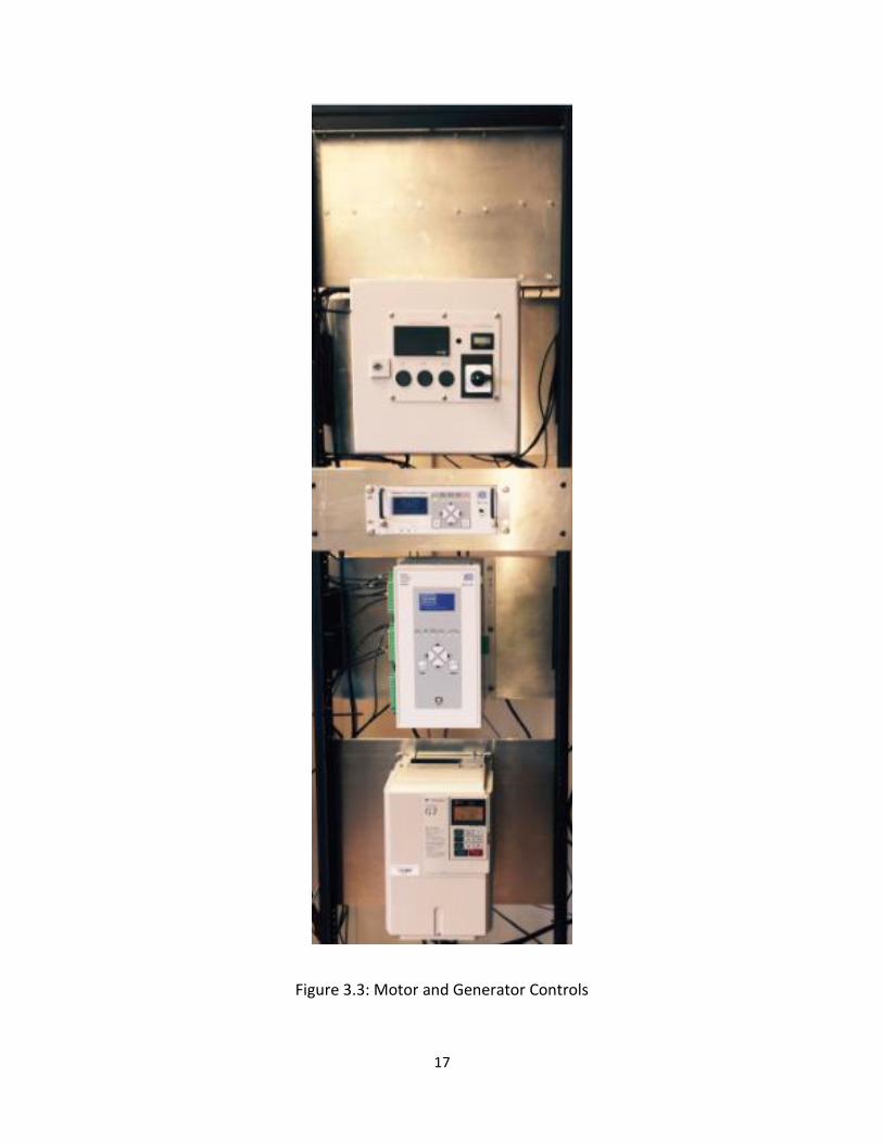
3.3 Control Mechanism

In order to control a single generation unit, many different control devices must operate

in conjunction with each other. Control components were mounted on a single rack with

casters.

The generator was equipped with a voltage regulator, but this was disconnected due to

the lack of flexibility. A Basler DECS-250 was purchased to control the generator field. This was

purchased without the Power Systems Stabilizer module. The generator can be operated in 2

basic modes, Automatic Voltage Regulation (AVR) or Manual. AVR monitors and maintains the

generator terminal voltage. Manual keeps the field current or voltage, depending on the

control method, constant regardless of bus voltage or load changes. Inputs include generator

terminal voltage, generator current, trip command from relay, and PSS gain from dSPACE . The

only outputs is DC current to generator brushless field.

17

Figure 3.3: Motor and Generator Controls

18

Figure 3.4: Generator Voltage Regulator

Figure 3.5: Generator Field Loop Diagram

19

Figure 3.6: PSS Gain Loop Diagram

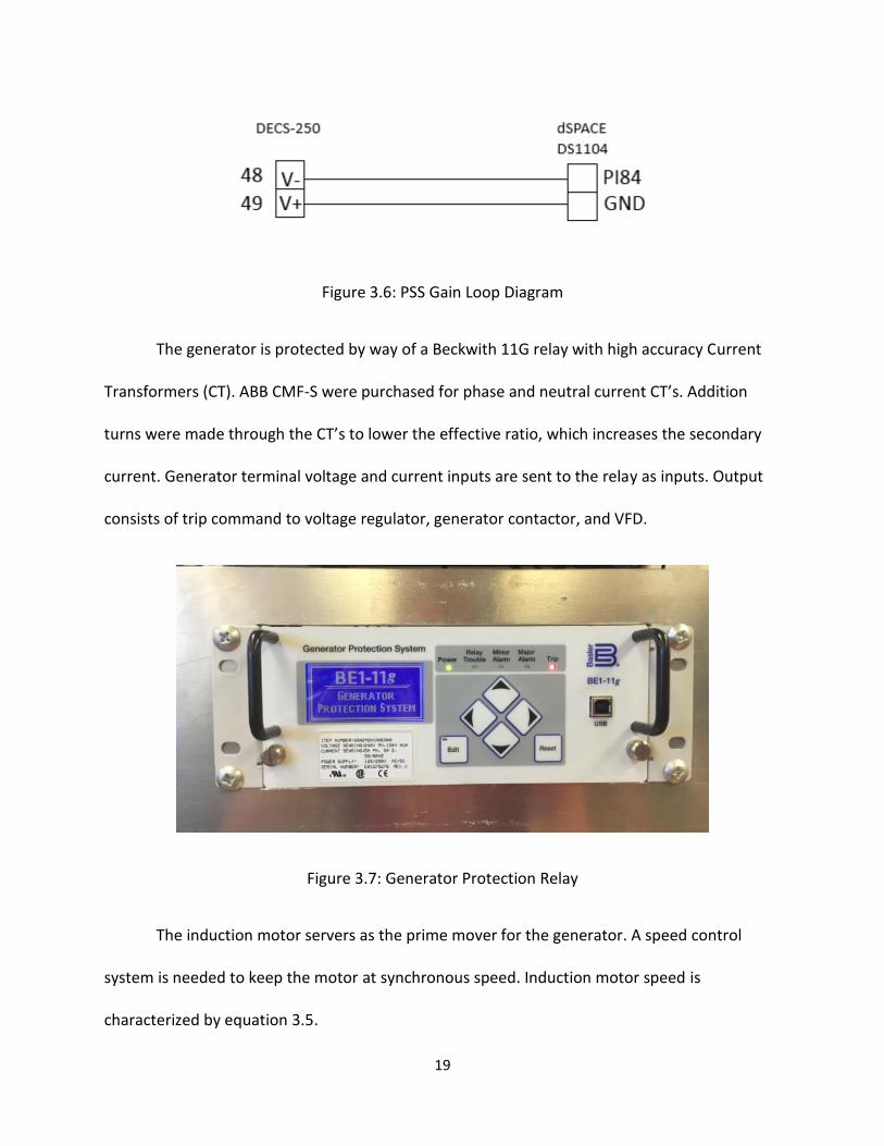
The generator is protected by way of a Beckwith 11G relay with high accuracy Current

Transformers (CT). ABB CMF-S were purchased for phase and neutral current CT’s. Addition

turns were made through the CT’s to lower the effective ratio, which increases the secondary

current. Generator terminal voltage and current inputs are sent to the relay as inputs. Output

consists of trip command to voltage regulator, generator contactor, and VFD.

Figure 3.7: Generator Protection Relay

The induction motor servers as the prime mover for the generator. A speed control

system is needed to keep the motor at synchronous speed. Induction motor speed is

characterized by equation 3.5.

20

𝑛 = 𝑛1 (1 − 𝑠) (3.5)

𝑤ℎ𝑒𝑟𝑒

𝑛 = 𝑆𝑝𝑒𝑒𝑑 𝑜𝑓 𝑅𝑜𝑡𝑜𝑟 (𝑅𝑃𝑀)

n1=Speed of Magnetic Flux (RPM)

𝑠 = 𝑆𝑙𝑖𝑝 (𝑅𝑃𝑀)

To combat the inherent slip and speed reductions caused by increased loading, a

Variable Frequency Drive was installed. A 480V VFD was specified, so a step up transformer was

purchased to accommodate the lower voltages present in the lab. PID control loop was installed

with an encoder to keep the machine at synchronous speed. Input to PID control is the

generator quadrature encoder.

Figure 3.8: Speed Signal Loop Diagram

21

Figure 3.9: Torque versus Speed on Variable Frequency Control

A VFD controls the speed of the motor similarly to a gas or steam turbine powered

generator. Multiple control modes can be utilized and key variables can be adjusted to change

the performance of the prime mover. Flux Vector control was chosen due to precise speed and

torque control as well as feedback utilization. The encoder signal is sent to the VFD as a

reference value.

3.4 Power System Stabilizer

The Simulink Generic Power System Stabilizer was implemented via dSPACE to show

proof of concept. The PSS utilizes a single speed deviation input and exports a stabilized voltage

per unit value to send to the voltage regulator as a ± 5VDC. The voltage regulator then

interprets this as a gain function to adjust the generator terminal voltage to. Voltage regulator

controls the DC field current of the synchronous generator. As generator terminal voltage

22

decrease, electric power delivered from the generator decreases as well.

Figure 3.10: Simulink PSS Block Diagram

PSS was executed in dSPACE by reading and determining speed from the quadrature

encoder. Speed deviation is amplified by to increase the sensitivity of PSS control through a

gain block. Wash-out is a low pass filter designed to remove harmonics above fundamental.

Lead-lag provides phase lead compensation to account for inherent phase lag. Limiter is used to

keep the PSS control from excessive manipulator of generator terminal voltage.

𝛥𝑌𝑃𝑆𝑆 in equation 3.6, is added into the voltage regulator signal, and A Matrix is

modified to create equation 3.8.

𝛥𝐸𝑓𝑑 = 𝐾𝐴

1+𝑠𝑇𝐴(𝛥𝑉𝑟𝑒𝑓 − 𝛥𝑉𝑇 + 𝛥𝑦𝑃𝑆𝑆) (3.6)

𝛥�̇�𝑃𝑆𝑆 = −1

𝑇2𝛥𝑦𝑃𝑆𝑆 +

𝐾𝑃𝑆𝑆

𝑇2

𝛥𝜔

𝜔𝑠+

𝑇1𝐾𝑃𝑆𝑆

𝑇2

𝛥�̇�

𝜔𝑠 (3.7)

𝛥�̇�𝑃𝑆𝑆 = −1

𝑇2𝛥𝑦𝑃𝑆𝑆 +

𝐾𝑃𝑆𝑆

𝜔𝑠𝑇2𝛥𝜔 +

𝑇1𝐾𝑃𝑆𝑆

2𝐻𝑇2(𝛥𝑃𝑚 − 𝐾1𝛥𝛿 − 𝐾2𝛥𝐸′

𝑞) (3.8)

PSS constants are then chosen by utilizing an arbitrary number for 𝑇2 and performing

equations 3.9 and 3.10. 𝐾𝑃𝑆𝑆 is typically set higher than the calculated value, but this gives a

good starting point before commissioning.

23

𝑇1 =tan (𝑡𝑎𝑛−1(𝜔𝑇2)−𝜑𝑃𝑆𝑆)

𝜔 (3.9)

𝐾𝑃𝑆𝑆 =1

|𝐺𝑃𝑆𝑆(𝑗𝜔)||𝐻(𝑗𝜔)| (3.10)

3.5 Transmission Lines and Loads

The lab grid is modeled after the IEEE 14 bus arrangement shown in Figure 3.8, whereas

the impedance matrix is shown in Appendix A. Lines and load can be created by utilizing

capacitors, iron core inductors, and high resistance wire.

Figure 3.11: IEEE 14 Bus One Line Diagram

24

3.6. Photo Voltaic Cells

A PV system was specified to connect to the lab system. The system must operate in the

off-grid and on-grid modes. This requires a battery system to be connected in order to supply

power during times where power production momentarily dips to low levels, such as when a

cloud passes overhead. To better model typical PV generation, single phase inverters with a

wide range of control options were selected.

25

CHAPTER 4: EXPERIMENTS

4.1 Simulation Model

A software model was created to replicate the physical lab model. Simulink has an

excellent library of devices. Figure 4.1 shows the full model with includes the VFD, motor,

generator, voltage regulator, and PSS. Scopes were added to display trends.

26

Figure 4.1: Simulink Block Diagram

27

Figure 4.2: Simulink AVR Exciter Block Diagram

Figure 4.3: Simulink PSS Block Diagram

The model was executed with PSS and without. The model include startup of the

equipment with 2 kW of load, increase to 4 kW of load, and decrease to 2 kW of load. Notice

the oscillations observed in Figures 4.4 and 4.5. PSS greatly reduced the oscillations amplitude

and duration.

28

Figure 4.4: Simulink Simulation without PSS (Graphs arranged top to bottom: VFD Vab, Rotor Speed (Wm), Electromagnetic Torque (Nm), Rotor Speed (pu), Output Active Power (pu),

Output Reactive Power (pu), Generator Vab)

29

Figure 4.5: Simulink Simulation with PSS (Graphs arranged top to bottom: VFD Vab, Rotor Speed (Wm), Electromagnetic Torque (Nm), Rotor Speed (pu), Output Active Power (pu), Output

Reactive Power (pu), Generator Vab)

30

4.2 Physical Model

The lab was used to perform a physical model for the network described in section 3.5.

The VFD was operated at 60.07 Hz in to allow for slip caused by the induction motor. The

generator was connected to a static load bank operating unsynchronized from the public grid.

The load bank was set to 2 KW and an additional 4 KW was momentarily added to create

system disturbances.

Figure 4.6: Load Bank

31

PSS was implemented via dSPACE. dSPACE utilized an encoder input and delivered an

analog output voltage to the voltage regulator to adjust the gain function. Trends were

recorded in dSPACE at a sampling rate of 10 kHz.

Figure 4.7: dSPACE Control Graphic

The generator was operated to observe the impact of PSS on the lab setup. At light

loads, the encoder output fluctuated, which were possibly caused by rotor dynamics. Once

additional load was added the effects decreased. Figures 4.8 and 4.9 shows the impact of PSS.

Observe how the speed was held closer to desired 1800 rpm when PSS was utilized and

oscillations were of lower frequency.

32

Figure 4.8: Generator Speed and Gain with PSS Implemented

Figure 4.9: Generator Speed without PSS Implemented

To better observe the characteristics of PSS, we must observe the points of interest

more closely. Figure 4.10 is a capture of load suddenly added to the generator. Since PSS is

reactive to disturbances rather than proactive, the speed will sharply decrease for both cases.

33

Notice the speed is maintained higher when PSS is used and the recovery time from the event is

much quicker. Figure 4.11 shows the impact of suddenly removing load from the generator.

Notice that the speed to kept lower when PSS is utilized and the response time is slightly

quicker.

Figure 4.10: Speed versus Time with and without PSS with Increasing Load

Figure 4.11: Speed versus Time with and without PSS with Decreasing Load

34

4.3 Conclusion

The lab performed well under a purely resistive load. All tests were perform in

isochronous mode, but the system was synchronized on several occasions for other

experiments. PSS was originally to be run through a National Instruments controller. Due to IT

issues with driver and lack of training on the software, dSPACE was utilized instead. Future

experiments will require a high inertia constant kVA load, such as an induction motor. Load can

be controlled by driving a blower with an air dampener.

On several occasions, the generator was synchronized to the grid through a three-phase

contactor. Generator protective relay performed the synchronizing check function to ensure

the systems where in synchronization. VFD was changed to torque mode to allow finer tuning

of the load. Load was successfully varied from full motoring to full generation. However, one

phase was operating at a much higher current. This is likely due to high loading on that specific

phase in the Electrical Engineering building. A system operating in isochronous mode has much

larger impedance than grid.

35

CHAPTER 5: SUMMARY

LSU Power Systems Lab was designed to handle a variety of experiments. These

experiments can be performed with software or physical components. The lab can operate on-

grid or off-grid, and loads can easily be changed. Generator parameters can be modified to best

replicate the study’s needs. This project challenged me greatly, and I have learned a lot.

36

REFERENCES

[1] Shahab Mehraeen, S. Jagannathan, Mariesa L. Crow, “Novel Dynamic Representation and Control of Power Systems With FACTS Devices”, IEEE Transactions on Power Delivery, Vol 25 No 3, pp. 1542-1554 [2] Shahab Mehraeen, S. Jagannathan, Mariesa L. Crow, “Power System Stabilization Using Adaptive Neural Network-Based Dynamic Surface Control”, IEEE Transactions on Power Delivery, Vol 26 No 2, pp. 669-680 [3] Basler Electric, Instruction Manual for Digital Excitation Control System DECS-250, July 2013 [5] Basler Electric, Instruction Manual for BE1-11g Generator Protection System, February 2017 [6] Yaskawa, G7 Drive Technical Manual, July 2008 [7] C.R. Mason, Art & Science of Protective Relaying - Online Version: http://www.gegridsolutions.com/multilin/notes/artsci/index.htm

[8] IEEE Guide for Synchronous Generator Modeling Practices and Applications in Power System Stability Analyses, IEEE std 1110-2002, 2002 [9] IEEE Recommended Practice for Excitation Models for Power System Stability Studies, IEEE std 421.5-2016, 2016 [10] IEEE Standard Definitions for Excitation Systems of Synchronous Machines, IEEE std 421.1-2007, 2007 [11] Zia A Yamayee, Juan L. Bala, Jr., Electromechanical Energy Devices and Power Systems, John Wiley & Sons, Inc., 1994. pp. 221-438.

37

APPENDIX: IEEE 14 Bus

Table A.1 IEEE 14 Bus - Load

Bus Voltage PL QL

1 1.0600 0.0000 0.0000

2 1.0450 0.2170 0.1270

3 1.0100 0.9420 0.1900

4 1.0000 0.4780 0.0390

5.00% 1.0000 0.0760 0.0160

5 1.0000 0.0000 0.0000

6 1.0700 0.1120 0.0750

7 1.0000 0.0000 0.0000

8 1.0900 0.0000 0.0000

9 1.0000 0.2950 0.1660

10 1.0000 0.0900 0.0580

11 1.0000 0.0350 0.0180

12 1.0000 0.0610 0.0160

13 1.0000 0.1350 0.0580

14 1.0000 0.1490 0.0500

38

Table A.2 IEEE 14 Bus - Line Impedance

From Bus To Bus R X Y

1.0000 2.0000 0.01938 0.05917 0.0528

1.0000 8.0000 0.05403 0.22304 0.0492

2.0000 3.0000 0.04699 0.19797 0.0438

2.0000 6.0000 0.05811 0.17632 0.0374

2.0000 8.0000 0.05695 0.17388 0.0340

3.0000 6.0000 0.06701 0.17103 0.0346

6.0000 8.0000 0.01335 0.04211 0.0128

6.0000 7.0000 0.00000 0.20912 0.0528

6.0000 9.0000 0.00000 0.55618 0.0492

8.0000 4.0000 0.00000 0.25202 0.0438

4.0000 11.0000 0.09498 0.19890 0.0374

4.0000 12.0000 0.12291 0.25581 0.0340

4.0000 13.0000 0.06615 0.13027 0.0346

7.0000 5.0000 0.00000 0.17615 0.0128

7.0000 9.0000 0.00000 0.11001 0.0528

9.0000 10.0000 0.03181 0.08450 0.0492

9.0000 14.0000 0.12711 0.27038 0.0438

10.0000 11.0000 0.08205 0.19207 0.0374

12.0000 13.0000 0.22092 0.19988 0.0340

13.0000 14.0000 0.17093 0.34802 0.0346

Table A.3 IEEE 14 Bus with Load Components Specified

Voltage PL (KW) QL (KVAR) R (Ω) X(Ω) L (H) C (microF)

254.4 0 0 0 0 0 0

250.8 1.562 0.914 40.259 68.789 0.182468 0

242.4 6.782 1.368 8.663 42.952 0.113933 0

240.0 3.442 -0.281 16.736 -205.128 0 12.931

240.0 0.547 0.115 105.263 500.000 1.326291 0

Table cont.

39

240.0 0.000 0.000 0.000 0.000 0 0

256.8 0.806 0.540 81.779 122.123 0.32394 0

240.0 0.000 0.000 0.000 0.000 0 0

261.6 0.000 0.000 0.000 0.000 0 0

240.0 2.124 1.195 27.119 48.193 0.127835 0

240.0 0.648 0.418 88.889 137.931 0.365873 0

240.0 0.252 0.130 228.571 444.444 1.178926 0

240.0 0.439 0.115 131.148 500.000 1.326291 0

240.0 0.972 0.418 59.259 137.931 0.365873 0

240.0 1.073 0.360 53.691 160.000 0.424413 0

Table A.4 IEEE 14 Bus with Line Components Specified

Bus To Bus R L(mH) C (microF) C/2 (mF)

1.0000 2.0000 0.155 1.2556 17.5070 8.754

1.0000 8.0000 0.432 4.7331 16.3134 8.157

2.0000 3.0000 0.376 4.2011 14.5229 7.261

2.0000 6.0000 0.465 3.7416 12.4008 6.200

2.0000 8.0000 0.456 3.6898 11.2735 5.637

3.0000 6.0000 0.536 3.6294 11.4724 5.736

6.0000 8.0000 0.107 0.8936 4.2441 2.122

6.0000 7.0000 0.000 4.4377 17.5070 8.754

6.0000 9.0000 0.000 11.8025 16.3134 8.157

8.0000 4.0000 0.000 5.3480 14.5229 7.261

4.0000 11.0000 0.760 4.2208 12.4008 6.200

4.0000 12.0000 0.983 5.4285 11.2735 5.637

4.0000 13.0000 0.529 2.7644 11.4724 5.736

7.0000 5.0000 0.000 3.7380 4.2441 2.122

7.0000 9.0000 0.000 2.3345 17.5070 8.754

Table cont.

40

9.0000 10.0000 0.254 1.7931 16.3134 8.157

9.0000 14.0000 1.017 5.7376 14.5229 7.261

10.0000 11.0000 0.656 4.0759 12.4008 6.200

12.0000 13.0000 1.767 4.2416 11.2735 5.637

13.0000 14.0000 1.367 7.3852 11.4724 5.736

41

VITA

Kevin Daniel Wellman was born 1988, in Gulfport, MS. He received his Bachelor of

Science from Mississippi State University in 2011. His career started in 2011 after graduation.

He worked for The Dow Chemical Company as a Run Plant Engineer for Energy Systems in

Plaquemine, LA from 2011 until 2015. In 2015, he transferred with the company to Houston, TX

to become a site leverage Electrical Maintenance Engineer. He plans to be awarded the degree

of Master of Science in Electrical Engineering in August of 2017.