Experimental Measurements of LiFePO Battery Thermal

Experimental Measurements of

LiFePO4 Battery

Thermal Characteristics

by

Scott Mathewson

A thesis

presented to the University of Waterloo

in fulfillment of the

thesis requirement for the degree of

Master of Applied Science

in

Mechanical Engineering

Waterloo, Ontario, Canada, 2014

© Scott Mathewson 2014

ii

Author's Declaration

I hereby declare that I am the sole author of this thesis. This is a true copy of the thesis, including any

required final revisions, as accepted by my examiners.

I understand that my thesis may be made electronically available to the public.

Scott Mathewson

iii

Abstract

A major challenge in the development of next generation electric and hybrid vehicle technology is the

control and management of heat generation and operating temperatures. Vehicle performance, reliability

and ultimately consumer market adoption are integrally dependent on successful battery thermal

management designs. It will be shown that in the absence of active cooling, surface temperatures of

operating lithium-ion batteries can reach as high as 50 °C, within 5 °C of the maximum safe operating

temperature. Even in the presence of active cooling, surface temperatures greater than 45 °C are

attainable. It is thus of paramount importance to electric vehicle and battery thermal management

designers to quantify the effect of temperature and discharge rate on heat generation, energy output, and

temperature response of operating lithium-ion batteries. This work presents a purely experimental thermal

characterization of thermo-physical properties and operating behavior of a lithium-ion battery utilizing a

promising electrode material, LiFePO4, in a prismatic pouch configuration.

Crucial to thermal modeling is accurate thermo-physical property input. Thermal resistance measurements

were made using specially constructed battery samples. The thru-plane thermal conductivity of LiFePO4

positive electrode and negative electrode materials was found to be 1.79 ± 0.18 W/m°C and 1.17 ± 0.12

W/m°C respectively. The emissivity of the outer pouch was evaluated to enable accurate IR temperature

detection and found to be 0.86.

Charge-discharge testing was performed to enable thermal management design solutions. Heat generated

by the battery along with surface temperature and heat flux at distributed locations was measured using a

purpose built apparatus containing cold plates supplied by a controlled cooling system. Heat flux

measurements were consistently recorded at values approximately 400% higher at locations near the

external tabs compared to measurements taken a relatively short distance down the battery surface.

The highest heat flux recorded was 3112 W/m2 near the negative electrode during a 4C discharge at 5 °C

operating temperature. Total heat generated during a 4C discharge nearly doubled when operating

temperature was decreased from 35 °C to 5 °C, illustrating a strong dependence of heat generation

mechanisms on temperature. Peak heat generation rates followed the same trend and the maximum rate of

90.7 W occurred near the end of 5 °C, 4C discharge rate operation. As a result, the maximum value of

total heat generated was 41.34 kJ during the same discharge conditions. The effect of increasing discharge

rate from 1C to 4C caused heat generation to double for all operating temperatures due to the increased

ohmic heating.

iv

Heat generation was highest where the thermal gradient was largest. The largest gradient, near negative

electrode current collector to external tab connection and was evaluated using IR thermography to be

0.632 °C/mm during 4C discharge with passive room temperature natural convection air cooling. Battery

designs should utilize a greater connection thickness to minimize both electrical resistance and current

density which both drive the dominant mode of heat generation, ohmic heating. Otherwise cooling

solutions should be concentrated on this region to minimize the temperature gradient on the battery.

v

Acknowledgements

I would first like to express my sincere gratitude to Dr. J. Richard Culham for his supervision, guidance

and patience during this study. The opportunity to work in the Microelectronics Heat Transfer Laboratory

(MHTL) has been a very rewarding experience made only possible by him.

I’d like to thank my peer, Satyam Panchal for his help in developing and running experiments. He always

brightened my spirits and reminded me to continue moving forward. He is truly one of the nicest people

I’ve ever had the pleasure of working with.

A special note of appreciation is owed to Dr. Fowler for enabling me to work within his lab and with his

students. I could not have completed this work without his support. I graciously extend that thanks to all

his students as well.

Finally, thanks to my family and friends. Thank you to my Mother for supporting me in every way

possible, and to my Uncle, Dr. K. Negus for his guidance and faith in me. It is to my family that I

dedicate this work, for their love, patience and understanding.

vi

Table of Contents

Author's Declaration .................................................................................................................................. ii

Abstract ........................................................................................................................................................ ii

Acknowledgements ..................................................................................................................................... v

Table of Contents ....................................................................................................................................... vi

List of Tables .............................................................................................................................................. ix

List of Figures ............................................................................................................................................ xii

Nomenclature ........................................................................................................................................... xvi

Terms and Definitions ............................................................................................................................ xvii

Introduction ......................................................................................................................... 1 Chapter 1

1.1. Electric Vehicle Batteries ........................................................................................................... 1

1.2. Motivation .................................................................................................................................... 2

1.3. Problem Statement ...................................................................................................................... 3

1.4. Outline .......................................................................................................................................... 4

Background and Literature Review .................................................................................. 5 Chapter 2

2.1. Lithium-Ion Batteries ................................................................................................................. 5

2.1.1. Positive Electrode Chemistry ................................................................................................ 7

2.1.2. Negative Electrode Chemistry .............................................................................................. 8

2.1.3. Electrolyte ............................................................................................................................. 9

2.1.4. Separator Materials ............................................................................................................. 10

2.1.5. Current Collectors ............................................................................................................... 11

2.1.6. Battery Construction ........................................................................................................... 11

2.2. Temperature Rise and Heat Generation of Lithium-ion Batteries ....................................... 16

2.2.1. Thermal Models .................................................................................................................. 17

2.2.2. Experimental Works ........................................................................................................... 31

2.3. Summary .................................................................................................................................... 37

Experimental Study .......................................................................................................... 39 Chapter 3

3.1. Thermal Conductivity Experiment ......................................................................................... 40

3.1.1. Batteries .............................................................................................................................. 40

vii

3.1.2. Thermal Resistance Test Stand ........................................................................................... 41

3.1.3. Procedure ............................................................................................................................ 43

3.1.4. Test Plan .............................................................................................................................. 45

3.1.5. Analysis Method ................................................................................................................. 46

3.2. Heat Generation and Cooling Experiment ............................................................................. 48

3.2.1. Batteries .............................................................................................................................. 48

3.2.2. Apparatus ............................................................................................................................ 49

3.2.3. Procedure ............................................................................................................................ 58

3.2.4. Plan ..................................................................................................................................... 59

3.2.1. Analysis Method ................................................................................................................. 61

3.3. Thermo-graphic Experiment ................................................................................................... 66

3.3.1. Batteries .............................................................................................................................. 66

3.3.2. Apparatus ............................................................................................................................ 66

3.3.3. Procedure ............................................................................................................................ 68

3.3.4. Plan ..................................................................................................................................... 68

3.3.5. Analysis Method ................................................................................................................. 69

Experimental Results and Discussion ............................................................................. 72 Chapter 4

4.1. Thermal Conductivity Results ................................................................................................. 73

4.1.1. Thermal Resistance ............................................................................................................. 73

4.1.2. Effective Thermal Conductivity of Samples ....................................................................... 77

4.2. Heat Generation and Cooling Results ..................................................................................... 80

4.2.1. Effect of Discharge Rate and Operating Temperature on Battery Temperature ................. 80

4.2.2. Effect of Discharge Rate and Operating Temperature on Heat Generation ........................ 85

4.2.3. Effect of Discharge Rate and Operating Temperature on Discharge Capacity ................... 92

4.3. Thermo-graphic Results ........................................................................................................... 94

4.3.1. Emissivity Measurement ..................................................................................................... 94

4.3.2. Temperature Response ........................................................................................................ 94

4.3.3. Temperature Gradient ......................................................................................................... 95

4.3.4. Thermal Images................................................................................................................... 98

Conclusions ...................................................................................................................... 103 Chapter 5

5.1. Summary .................................................................................................................................. 103

5.2. Recommendations ................................................................................................................... 105

References ................................................................................................................................................ 106

viii

Appendix A: Experimental Uncertainty ............................................................................................... 112

A.1. Method ......................................................................................................................................... 112

A.2. Experiment 1 Uncertainties ........................................................................................................ 113

A.2.1. Thermal Joint Resistance ....................................................................................................... 113

A.2.2. Thermal Conductivity ............................................................................................................ 113

A.2.3. Summary of Experiment 1 Uncertainty ................................................................................. 114


A.3.1. Average Surface Temperature ................................................................................................ 115

A.3.2. Heat Generation ..................................................................................................................... 116



A.4.1. IR Temperature ...................................................................................................................... 122

A.4.2. Temperature Response ........................................................................................................... 122

A.4.3. Thermal Gradient ................................................................................................................... 123


Appendix B: Experiment 1 Data Summary .......................................................................................... 125

Appendix C: Experiment 2 Results ....................................................................................................... 134

C.1. Effect of Cooling Temperature on Heat Generation ................................................................ 135

C.2. Discharge Data Tables ................................................................................................................ 137

ix

List of Tables

Table 2.1: Common lithium salts for use in electrolytes and their major disadvantages [15] .................... 10

Table 2.2: Compiled thermo-physical properties from literature [24], [25], [26] ....................................... 15

Table 2.3: Lumped thermo-physical properties from literature [6], [24], [25] ........................................... 16

Table 2.4: Compiled results from article (‘x’ represents discharge rate) [44] ............................................ 32

Table 3.1: Manufacturer specifications of 20Ah LiFePO4 Battery ............................................................. 41

Table 3.2: Planned samples for thermal conductivity measurements ......................................................... 45

Table 3.3: Test conditions for thermal conductivity measurements ........................................................... 46

Table 3.4: Spatial locations of thermocouples (dist. from bottom left corner of battery) ........................... 52

Table 3.5: Spatial locations of heat flux sensor centre-points (dist. from bottom left corner of battery) ... 54

Table 3.6: Cooling fluid properties ............................................................................................................. 56

Table 3.7: Planned tests for heat generation and temperature measurement experiments .......................... 59

Table 3.8: Actual coolant temperatures at inlet of cooling plates ............................................................... 60

Table 3.9: Discharge rates and equivalent current ...................................................................................... 61

Table 3.10: X and Y dimensions of thermcouple areas .............................................................................. 62

Table 3.11: Heat rate due to the ambient environment for the operating temperatures .............................. 65

Table 4.1: Thermal resistances of positive electrode samples with 1.38 MPa load condition .................... 74

Table 4.2: Thermal resistances of negative electrode samples with 1.38 MPa load condition ................... 75

Table 4.3: Layer-unit resistance summary .................................................................................................. 76

Table 4.4: Measured thicknesses of battery materials and tested samples at 1.38 MPa load pressure ....... 78

Table 4.5: Measured thicknesses of positive electrode samples at 1.38 MPa load ..................................... 79

Table 4.6: Measured thicknesses of negative electrode samples at 1.38 MPa load .................................... 79

Table 4.7: Determined thermal resistance and conductivity of individual layer-units ............................... 79

Table 4.9: Summary of maximum average surface temperatures of battery for all discharge rates and

coolant/operating temperatures tested ..................................................................................... 83

Table 4.10: Summary of maximum heat generation rates for four discharge rates at four operating

temperatures ............................................................................................................................ 86

Table 4.11: Summary of total heat produced for each discharge condition and cooling condition ............ 87

Table 4.12: Summary of average heat flux measured at 3 locations for all operating temperatures .......... 90

Table 4.13: Summary of peak heat flux measured at 3 locations for all operating temperatures ............... 91

Table 4.14: Summary of discharge capacities for the opearting temperatures and discharge rates tested.. 93

x

Table 4.15: Summary of discharge times for the operating temperatures and discharge rates tested ......... 93

Table 4.16: Average temperature response rate for each discharge condition and linear fit ...................... 95

Table 4.17: Average temperature gradient for each discharge condition and linear fit .............................. 96

Table 4.18: Average temperature gradient along top 46mm of evaluated lines for each discharge condition

and linear fit............................................................................................................................. 97

Table 4.19: Parameters of image series in following subsections............................................................... 98

Table A1: Average uncertainty in surface temperature for five operating temperatures .......................... 116

Table A2: Average uncertainties that give rise to uncertainty in Rayleigh number ................................. 120

Table B1: 7 layer positive electrode sample test results ........................................................................... 126

Table B2: 13 layer positive electrode sample test results ......................................................................... 127



Table B5: 7 layer negative electrode sample test results .......................................................................... 130

Table B6: 13 layer negative electrode sample test results ........................................................................ 131



Table C1: 1C Discharge data (5 °C Cooling, 240 second interval) .......................................................... 137

Table C2: 2C Discharge data (5 °C Cooling, 180 Second interval) .......................................................... 138


Table C4: 4C Discharge data (5 °C Cooling, 60 second interval) ............................................................ 140

Table C5: 1C Discharge data (15 °C Cooling, 240 second interval) ........................................................ 141

Table C6: 2C Discharge data (15 °C Cooling, 180 Second interval) ........................................................ 142




Table C10: 2C Discharge data (25 °C Cooling, 180 Second interval) ...................................................... 146

Table C11: 3C Discharge data (25 °C Cooling, 120 second interval) ...................................................... 147



Table C14: 2C Discharge data (35 °C Cooling, 180 Second interval) ...................................................... 150


xi

Table C16: 4C Discharge data (35 °C Cooling, 60 Second interval) ........................................................ 152

Table C17: 1C Discharge data (Air Cooling only, 240 second interval) .................................................. 153



Table C20: 4C Discharge data (Air Cooling only, 60 Second Interval) ................................................... 156

xii

List of Figures

Figure 1.1: Normalized discharge capacity fade at elevated temperatures. Discharge = C/3, RT = room

temperature [2] .......................................................................................................................... 2

Figure 1.2: Surface temperature profile of a lithium-ion pouch cell during 1C charge and 1C, 2C, 3C and

4C discharge rates. Natural convection air cooling only ........................................................... 3

Figure 2.1: Charge and discharge mechanism in Li-ion battery [4].............................................................. 6

Figure 2.2: Crystal structure of the lithium based species commonly used as battery electrodes. ............... 8

Figure 2.3: The hexagonal structure of a carbon layer used for Li-ion negative electrodes. Two

arrangements of layers are shown [4] ........................................................................................ 9

Figure 2.4: Schematic representation of multi-cell battery structure [21] .................................................. 12

Figure 2.5: Structure of wound cylindrical cells [22] ................................................................................. 13

Figure 2.6: Comparison of average temperatures (solid) and max/min temperatures (dotted) time variation

for prismatic (blue) and cylindrical (red) with mid-size PHEV10 US06 driving scenario [23]

................................................................................................................................................. 14

Figure 2.7: Single cell sandwich modeled by Pals and Newman [3] .......................................................... 17

Figure 2.8: A) Cell potential as a function of utilization and time for isothermal constant discharge current

at several temperatures. Dashed line is OCV of the cell. B) Heat generation rate as function of

utilization and time for isothermal constant discharge current [3] .......................................... 18

Figure 2.9: A) Adiabatic temperature rise as a function of utilization for several discharge current

densities. Dashed line is OCV of the cell. B) Heat generation rate as function of utilization

and time for adiabatic constant discharge current [3] .............................................................. 19

Figure 2.10: Schematic of model structure [26].......................................................................................... 20

Figure 2.11: Current density distributions and temperature distributions after 30 s of 5C discharge under

four different thermal conditions: isothermal, adiabatic, cooling same side as tabs, and

cooling opposite of tabs [26]. .................................................................................................. 21

Figure 2.12: Average cell temperature of cells in a 200 cell stack in 5 s intervals over a 60 s discharge at

5C [26]. .................................................................................................................................... 22

Figure 2.13: Steady-state 2-D temperature distribution in battery pack cooled by an air flow [30] ........... 23

Figure 2.14: Steady-state 2-D temperature distribution in an enclosed battery pack [30] .......................... 24

Figure 2.15: Simulated 1C discharge curves for a 6 Ah lithium-ion cell at different temperatures,

assuming isothermal operation ................................................................................................ 25

xiii

Figure 2.16: Schematic of Li-ion battery pack cooling arrangement evaluated by Karimi and Dehghan

[37] .......................................................................................................................................... 27

Figure 2.17: Temperature distributions in a prismatic pack for 4 cooling conditions. a) Silicon Oil, U-

pattern, h = 100 [W/m2 K], b) Air, Z-pattern, h = 250 [W/m

2 K], c) Silicon Oil, Z-pattern, h =

100 [W/m2 K], d) Air, Z-Pattern, h = 250 [W/m

2 K]............................................................... 28

Figure 2.18: The effect of PCM thermal management on thermal response of 8S2P battery packs [41] ... 29

Figure 2.19: Cell temperature increase for PHEV-20 battery pack under stressed discharge conditions

(Tamb = 40 °C, discharge rate = 6.67C) [39] ............................................................................ 30

Figure 2.20: Thermocouple locations on a 4.8 Ah prismatic battery used by Williford et al. [27] ............ 33

Figure 2.21: Test rig with cell holder and Peltier thermoelectric elements [45] ......................................... 33

Figure 2.22: Measured heat generation profiles of LiAl0.2Mn1.8O4-δF0.2 based 2325 coin cells discharged at

C/3 in four ambient temperatures [47] .................................................................................... 35

Figure 2.23: The curve of charge-discharge heat rate. (a) Discharge of 2C, (b) charge of 2C, (c) Discharge

of 1C, and (d) charge of 1C [48] ............................................................................................. 36

Figure 2.24: Images used to compare electro thermal model [28] .............................................................. 36

Figure 3.1: Commercial 20Ah LiFePO4/graphite prismatic battery ........................................................... 40

Figure 3.2: Schematic of test apparatus ...................................................................................................... 42

Figure 3.3: Image of pouching material and stack of electrode layers with seperator layers in between. .. 44

Figure 3.4: Simplified thermal resistance network for battery samples (HFM = ‘heat flux meter’) .......... 46

Figure 3.5: Breakdown of thermal resistance values on resistance-thickness plot ..................................... 47

Figure 3.6: Charge discharge test bench ..................................................................................................... 49

Figure 3.7: Schematic representation of charge discharge test stand .......................................................... 51

Figure 3.8: Keithley 2700 data logger and M7700 input module ............................................................... 52

Figure 3.9: Spatial arrangement of thermocouples ..................................................................................... 53

Figure 3.10: Spatial locations of heat flux sensor center-points ................................................................. 54

Figure 3.11: Schematic of cooling system flow from bath to cooling plate (P1,P2) inlets/outlets ............. 55

Figure 3.12: Cooling plate design provided by manufacturer..................................................................... 56

Figure 3.13: Exploded assembly of isolating rig built for active cooling tests. (Insulation not shown) ..... 57

Figure 3.14: Cold plate within compression rig. ......................................................................................... 58

Figure 3.15: Standard charge profile used in charge-discharge testing ...................................................... 60

Figure 3.16: Distribution of areas used to determine average surface temperature .................................... 62

Figure 3.17: Plot of ambient heat flow for the operating temperatures tested ............................................ 65

Figure 3.18: FLIR S60 ThermaCam [52] .................................................................................................... 66

xiv

Figure 3.19: Thermo-graphic experimental set-up showing (L) battery on stand and (R) battery and

camera positioning .................................................................................................................. 67

Figure 3.20: Photograph of Gier-Dunkle DB100 infra-red reflectometer .................................................. 67

Figure 3.21: Line locations where thermal gradient data was evaluated from IR Images .......................... 69

Figure 4.1: All thermal resistances measured ............................................................................................. 73

Figure 4.2: Positive electrode sample average thermal resistances at 1.38 MPa load pressure .................. 74

Figure 4.3: Negative electrode sample average thermal resistances at 1.38 MPa load pressure. ............... 75

Figure 4.4: Temperature response at each thermocouple during 1C discharge at 15 °C Operating

temperature .............................................................................................................................. 81


temperature .............................................................................................................................. 82


temperature .............................................................................................................................. 82

Figure 4.7: Maximum average surface temperatures of battery for all discharge rates and

coolant/operating temperatures tested ..................................................................................... 83

Figure 4.8: Difference in average surface temperature between start and end of discharges ..................... 84

Figure 4.9: Heat generation rates of LiFePO4 battery for four discharge rates at 25 °C ............................. 85

Figure 4.10: Total heat produced for each discharge condition and cooling condition .............................. 86

Figure 4.11: Heat flux sensor response during 1C and 4C discharge at 5 °C operating temperature. ........ 88

Figure 4.12: Effect of increased discharge rate on average heat flux [W/m2] measured at 3 different

locations for all operating temperatures .................................................................................. 89

Figure 4.13: Effect of increased discharge rate on peak heat flux [W/m2] measured at 3 different locations

all operating temperatures ....................................................................................................... 91

Figure 4.14: Effect of operating temperature on the discharge capacity of LiFePO4 Battery..................... 92

Figure 4.15: Average temperature rise of discharging battery along three vertical surface lines. .............. 94

Figure 4.16: Average temperature gradient along three vertical surface lines. ........................................... 96

Figure 4.17: Average temperature gradient for top 46 mm of negative electrode line ............................... 97

Figure 4.18: IR images of 2C discharge with passive cooling. Time after start of discharge is indicated

below each image, and estimated SOC is given in brackets ................................................. 100





xv

Figure B1: Thermal resitsance experimental data for 7 layer positive electrode sample .......................... 126

Figure B2: Thermal resitsance experimental data for 13 layer positive electrode sample ........................ 127



Figure B5: Thermal resitsance experimental data for 7 layer negative electrode sample ......................... 130

Figure B6: Thermal resitsance experimental data for 13 layer negative electrode sample ....................... 131



Figure C1: Effect of battery discharge rate on the heat generation profile of the test battery at an operating

temperature of 5 °C ................................................................................................................................... 135


temperature of 15 °C ................................................................................................................................. 135


temperature of 25 °C ................................................................................................................................. 136


temperature of 35 °C ................................................................................................................................. 136

xvi

Nomenclature

A = area [m2] T = temperature [°C]

cp = specific heat capacity [J/kg°C] th = thickness [m]

E = heat energy [J] t = time [s]

h = heat transfer coefficient [W/m2°C] V = cell voltage or cell potential [V]

I = current [A] ⁄ = temperature coefficient [V/°C]

k = thermal conductivity [W/m°C] ⁄ = temperature gradient [°C /m]

L = characteristic length [m]

m = mass [kg]

= mass flow rate [kg/s]

N = number

Pr = Prandtl number

q = heat flux [W/m2]

Q = heat generation rate [W]

R = thermal resistance [°C /W]

Ra = Rayleigh number

Greek Symbols

α = thermal diffusivity [m2/s]

β = thermal expansion coefficient

ε = emissivity

i = layer index

= density [kg/m³]

μ = dynamic viscosity [kg/ms]

ν = kinematic viscosity [m2/s]

Subscripts

∞ = ambient

b = battery

bs = battery surface

c = cell

conv = convection

e = electrical

f = fluid

gen = generated

i = layer index

n = negative electrode

oc = open circuit

p = positive electrode

rad = radiation

T = temperature

th = thermal

w = water

x,y,z = Cartesian coordinate directions

xvii

Terms and Definitions

Battery Cycle Consists of 1 complete charging process and 1 complete discharging process.

Charge Rate Charge rate is a measurement of the current applied to recharge the battery.

Applied current [A] divided by capacity of battery [Ah] gives the charge rate [h-1

].

For a fully discharged 100 Ah battery, a 1C charge rate would apply 100 A for 1

hour to reach 100% SOC.

Discharge Rate Discharge rate is a measurement of the current applied to discharge the battery.

Current drawn divided by capacity of battery [Ah] gives the discharge rate [h-1

].

For a fully discharged 100 Ah battery, a 1C charge rate would apply 100 A for 1

hour to reach 100% SOC.

Battery

Capacity

The coulometric capacity, the total amp-hours available when battery is discharged

at a certain discharge current (specified as a C-rate) from 100% SOC to the cut-off

voltage. Capacity is calculated by multiplying the discharge current (in Amp) by

the discharge time (in hours) and decreases with increasing C-rate.

Nominal

Energy

The “energy capacity” of the battery, the total watt-hours available when battery is

discharged at a certain discharge current (specified as a C-rate) from 100% SOC to

the cut-off voltage. Energy is calculated by multiplying the discharge power (in

watts) by the discharge time (in hours). Like capacity, energy decreases with

increasing C-rate.

Intercalation

The reversible inclusion of a chemical species (ion, molecule, etc.) between two

other chemical species.

Battery Cell A cell is the smallest, packaged form a battery can take and is generally on the

order of one to six volts

Battery Module A module consists of several cells generally connected in either series or parallel.

Battery Pack A battery pack is then assembled by connecting modules together, again either in

series or parallel.

State of Charge

(SOC)

The state of charge (SOC) is a percentage measure of charge remaining in a battery

relative to its predefined “full” and “empty” states. Manufacturers typically

provide voltages that represent when the battery is empty (0% SOC) and full

(100% SOC). SOC is generally calculated using current integration to determine

the change in battery capacity over time.

Depth of

Discharge

(DOD)

The depth of discharge (DOD) is a percentage measure of the amount of energy

extracted during a discharge process, compared to a fully charged state. Depth of

discharge is the compliment of state of charge (SOC). A battery at 60% SOC is

also at 40% DOD.

Cycle life Cycle life refers to the number of times a battery must be charged and discharged

before its nominal capacity falls below 80% (or some other predetermined

xviii

threshold) of its rated value. Cycle life is given for a particular DOD and

determined at specific charge and discharge conditions.

Open Circuit

Voltage (OCV)

The open circuit voltage (OCV) is the voltage when no current is flowing in or out

of the battery, and, hence no reactions occur inside the battery. OCV is a function

of state-of-charge and is expected to remain the same during the life-time of the

battery. However, other battery characteristics change with time, e.g. capacity is

gradually decreasing as a function of the number of charge-discharge cycles.

Terminal

Voltage (V)

The voltage between the battery terminals with load applied. Terminal voltage

varies with SOC and discharge/charge current.

Nominal

Voltage (V)

The reported or reference voltage of the battery, also sometimes thought of as the

“normal” voltage of the battery.

Cut-off Voltage

(V)

The minimum allowable voltage. It is this voltage that generally defines the

“empty” state of the battery

Charge Voltage

(V)

The voltage that the battery is charged to when charged to full capacity. Charging

schemes generally consist of a constant current charging until the battery voltage

reaches the charge voltage, then constant voltage charging, allowing the charge

current to taper until it is very small.

Specific Energy

(Wh/kg)

The “energy capacity” of the battery, the total watt-hours available when a battery

is discharged at a certain discharge current (specified as a C-rate) from 100% SOC

to the cut-off voltage. Energy is calculated by multiplying the discharge power (in

watts) by the discharge time (in hours). Like capacity, energy decreases with

increasing C-rate.

Energy Density

(Wh/L)

The energy density of a battery is expressed as a nominal energy per unit volume,

such as Wh/L. It is highly dependent on the battery chemistry and packaging.

Power Density

(W/L)

The power density of a battery is expressed as a nominal power per unit volume,

such as W/L or kW/L. It is highly dependent on the battery chemistry and

packaging.

PHEV Plug-in hybrid electric vehicle.

SOD Start of discharge

EOD End of discharge

1

Introduction Chapter 1

Introduction

For nearly a decade, electrified powertrain vehicles have been available for purchase in North America.

Steady growth in market share continues as the benefits of electrified systems over conventional

powertrains become increasingly valued. Concern for the environment and increasing cost of fossil fuel

based transportation has driven consumers to demand vehicles that produce minimal carbon emissions

and utilize power from the utility based electrical grid. Vehicle manufacturers have responded with three

powertrain designs that utilize electrification in some or all of the energy storage mechanisms. These

systems can be classified into two categories defined by the battery management scheme: charge

sustaining (CS) and charge depleting (CD).

Common to all proposed and current electrical vehicle designs are the presence of batteries to provide

electrochemical energy storage. A number of batteries are connected to produce a battery pack with

desired electrical characteristics, such as output voltage and available maximum current. The performance

of electrified vehicles depends on the performance of their battery packs. Vehicle range and acceleration

are specifications that depend on adequate and consistent battery performance. Due to the electrochemical

nature of the batteries, the temperature of operation affects their output.

In order to establish control methods that maximize battery performance, the effects of operating

temperature and thermal output of discharging batteries must be known. This research is primarily

concerned with the thermal effects and thermal behavior of individual lithium-ion (Li-ion) batteries.

1.1. Electric Vehicle Batteries

Since the electric vehicle’s invention electrochemical batteries primarily have been used to store or

release the energy used for propulsion. Energy is transferred to or from the battery by creating or breaking

chemical bonds in a controlled way, such that electrons flow through an external circuit.

2

The commercially available and widely used rechargeable batteries are lead-acid, nickel cadmium, nickel

metal hydride, lithium-ion, and lithium-ion polymer batteries. Lithium-ion batteries are a relatively new

battery technology currently undergoing immense growth and development. This work focuses on a

particular lithium-ion battery electrode chemistry, LiFePO4. Details about lithium-ion battery operation

and electrode pairs are given in Section 2.1.

1.2. Motivation

Electrochemical battery reactions are strongly coupled to temperature [1]. At low temperatures, higher

activation energy is needed for the electrochemical reactions to take place and ion diffusion rates are

slow. These two factors lead to a loss of apparent capacity and delivered power. Generally, when

operating temperature is restored to nominal levels, the capacity and power delivery are recovered. When

the battery is subjected to nominal discharge rates, low temperature on its own does not have any

permanent effect on capacity fading, but during charging conditions, lithium plating is likely to occur due

to a decreased intercalation rate at the anode compared to the cathode de-intercalation rate [1].

Continued cycling at elevated temperatures can cause irreversible decreases to the discharge capacity of

Li-ion batteries [2]. In Figure 1.1, the effect of cycling at elevated temperatures on capacity is shown.

FIGURE 1.1: NORMALIZED DISCHARGE CAPACITY FADE AT ELEVATED TEMPERATURES. DISCHARGE =

C/3, RT = ROOM TEMPERATURE [2]

For a given battery technology, temperature limits of operation are provided to minimize degradation and

preserve battery life. This is of great concern to automotive manufacturers as the battery is a major

contributor to the cost of Electric Vehicles (EV).

Furthermore, automotive manufacturers are pressured to increase vehicle range and performance. This is

accomplished by increasing pack capacity and available current draw. This becomes problematic as the

3

heat generation mechanisms are strongly coupled to current density [3], and increased energy density

implies decreased surface area for cooling. Whereas before, packs were simply oversized to accomplish

the required range while limiting current draw, packs must now be optimized for cooling to ensure long

life and good performance of the overall vehicle.

Lithium-ion battery heat generation is strongly coupled to discharge rate (current flow). Figure 1.2 was

prepared by measuring the temperature on the surface of a single battery discharging at 4 increasing

constant current rates. The specified operating temperature range for the particular battery used was -30

°C to 55 °C. With 4C discharges, and no active cooling the battery easily reaches temperatures above the

nominal operating range. Optimized cooling may have potential to increase overall electrical efficiency

and resultant vehicle range by maintaining batteries at optimum temperature.

FIGURE 1.2: SURFACE TEMPERATURE PROFILE OF A LITHIUM-ION POUCH CELL DURING 1C CHARGE

AND 1C, 2C, 3C AND 4C DISCHARGE RATES. NATURAL CONVECTION AIR COOLING ONLY

1.3. Problem Statement

The present work is confined to the thermal characterization of LiFePO4 lithium-ion batteries designed for

automotive applications. The objective of this work is:

a) To design an apparatus that directly measures:

i) The surface temperature distribution of prismatic batteries undergoing discharge.

ii) The surface heat flux near the positive electrode, negative electrode, and at the center of

the prismatic cell surface, and

20

25

30

35

40

45

50

55

60

0 5000 10000 15000 20000 25000 30000 35000 40000

Tem

per

atu

re (

0C

)

Time (s)

3C

2C

4C

1C

4

iii) The heat removed from the battery by any cold plates used in the apparatus for different

discharge rates.

b) To produce data sets of temperature, heat fluxes and heat generation of LiFePO4 battery

undergoing discharges at different operating temperatures

c) To visually observe and report the locations of highest heat generation using infrared thermo-

graphic techniques

d) To examine the effect of discharge rate and operating temperature on battery discharge capacity.

e) To evaluate the thermal resistance and thermal conductivity (k) of the layered battery structure

and constituent layers

1.4. Outline

The presentation of this research has been organized in the following order:

Chapter 2, which follows, provides a description of the operation of lithium-ion batteries as well as a

literature review of existing lithium-ion battery thermal models and experimental programs that

incorporate empirical measurement of temperature and heat generation.

Chapter 3 details the experiments performed that generated the empirical data of interest. The details

include: Experimental set-ups, experimental plans and procedures. Also included in the subsections for

each experiment are the methods of analysis including any relationships, equations, and assumptions

applied.

Chapter 4 presents the analyzed results from the various experiments, including the thermal image series

generated from the third experiment listed in Chapter 3.

Chapter 5 contains a summary of the work performed, along with conclusions and recommendations from

this research.

Appendix A contains analysis of the uncertainty in each experiment.

Appendix B contains tables generated from the Experiment 1 data.

Appendix C contains tables generated from the Experiment 2 data.

5

Chapter 2

Background and Literature Review

2.1. Lithium-Ion Batteries

The electro-chemical and electro-thermal performance of lithium-ion batteries has been the focus of many

investigations in recent years, and the subject has been extensively treated analytically and numerically. A

single lithium-ion battery cell consists of two current conductors, a negative electrode, a separator and a

positive electrode. The electrodes are porous solids which consist of uniform size, spherical, active

particles and additives. The separator is a porous polymer membrane. All components are immersed in an

electrolyte. The electrodes and the electrolyte are involved in the charge and species balance that makes

up the electro-chemical reaction. The current conductors provide a path for electrons to flow through an

external circuit [4].

6

FIGURE 2.1: CHARGE AND DISCHARGE MECHANISM IN LI-ION BATTERY [4]

The electrodes are considered to be a composite material and the chemistry of the positive electrode

defines the type of Li-ion cell. The negative electrode is generally made out of graphite or a metal oxide.

The electrolyte can be liquid, polymer or solid. The separator is chemically porous to enable the transport

of lithium ions but electrically insulating to prevent the cell from internal short circuits.

Lithium battery reactions of this type operate by reversibly incorporating lithium in an intercalation

process. During charging, an applied potential across the electrodes causes lithium ions (Li+) to diffuse

from the cathode to the anode via the electrolyte. The ions fill voids in the cathode composite structure,

and cause a charge potential to be established between the two electrodes. When all the available lithium

ions intercalate into the positive electrode, the battery is considered to be fully charged.

During discharge, an external circuit is used to connect the electrodes and electrical current flows until the

charge potential is eliminated or the circuit is disconnected. These processes are shown in Figure 2.1 for a

Li-ion cell.

7

A note about electrode terminology: the positive electrode is the cathode during discharge as it is the

location of chemical reduction. The opposite reaction, oxidation, occurs at the negative electrode which is

the anode. The opposite is valid when an external voltage is applied and the battery is charging. Then, the

location of oxidation and reduction change and as such the positive electrode is no longer the cathode.

Within this work, electrodes will be primarily referred to by their polarity, and otherwise cathode is taken

to be the positive electrode, while anode is the opposite.

2.1.1. Positive Electrode Chemistry

Numerous commercially available lithium based electrode pairs have been identified. The positive

electrodes utilize a lithiated metal oxide or lithiated metal phosphate as the active material [4]. Three of

the most commonly used positive electrodes chemistries are discussed following. Images of the crystal

structures discussed are displayed in Figure 2.2.

LiCoO2: LiCoO2 is most the most commonly used cathode material [5]. Lithium ions are intercalated

between sheets of CoO2 with a theoretical specific capacity of 274 mAh/g [5]. The structure type of

LiCoO2 is an ordered rock salt-type structure shown in Figure 2.2A [4]. Due to an anisotropic structural

change that occurs at Li0.5CoO2, the realizable capacity is limited to about 140-160 mAh/g [6]. The

discharge capacity of LiCoO2 is good; 136 mAh/g at a 5C rate has been demonstrated with multiwall

carbon nanotube (CNT) augmented electrodes [6]. Despite the attractive electrical properties LiCoO2

cathodes, cobalt is relatively expensive compared to other transition metals such as manganese and iron.

As such research is motivated to develop more inexpensive options using these metals.

LiMn2O4 : LiMn2O4 is a promising cathode material with a cubic spinel structure, shown in Figure 2.2B.

The theoretical specific capacity is 148 mAh/g. Current designs achieve between 115 and 130 mAh/g at

modest discharge rates up to 1C [7]. LiMn2O4 is used commercially, particularly in applications that are

cost sensitive or require exceptional stability upon abuse. LiMn2O4 has lower capacity, 100 to 120 mAh/g,

slightly higher voltage, 4.0V, but has higher capacity loss on storage or cycling, especially at elevated

temperature, relative to cells that use LiCoO2 [4].

LiFePO4 : LiFePO4 is one of the most recent cathode materials to be introduced. Its olivine structure,

shown in Figure 2.2C, is very different from the layered and spinel structures of other lithium-ion

chemistries. The intercalation mechanism is also different, involving phase changes. LiFePO4 has a

specific capacity of about 160 mAh/g and an average voltage of 3.45V [4]. Recent developments have

approached the theoretical discharge capacity [8]. LiFePO4 has the added advantage of being inexpensive

and environmentally friendly.

8

A: LiCOO2 [9] B: LiMn2O4 [10] C: LiFePO4 [11]

FIGURE 2.2: CRYSTAL STRUCTURE OF THE LITHIUM BASED SPECIES COMMONLY USED AS BATTERY

ELECTRODES.

2.1.2. Negative Electrode Chemistry

Negative electrode materials are typically carbonaceous in nature. It is important for the material to be

able to hold large amounts of lithium without a significant change in structure, and have good chemical

and electrochemical stability with the electrolyte. Furthermore, it should be a good electrical and ionic

conductor, and be of relative low cost [4].

Graphite: Today, graphite in stacked layer is one of the most common anode materials in lithium-ion

batteries. An example of the structure of these layer stacks is shown in Figure 2.3. It is favored for its

small volume change during lithiation and delithiation [12]. With graphite electrodes, high coulombic

efficiencies of over 95% have been achieved, but they have a relatively low theoretical specific capacity

of 362 mAh/g [4]. Although this is already higher than the specific capacity of the commonly used

cathode materials, higher specific capacity carbon based electrodes are still desirable because they

contribute to a lower overall battery density.

9

FIGURE 2.3: THE HEXAGONAL STRUCTURE OF A CARBON LAYER USED FOR LI-ION NEGATIVE

ELECTRODES. TWO ARRANGEMENTS OF LAYERS ARE SHOWN [4]

Among carbonaceous materials, carbon nanotubes (CNTs) are the most promising materials being

developed. CNTs of the single walled variety can reversibly intercalate lithium ions with a maximum

composition of Li1.7C6, equivalent to a specific capacity of 632 mAh/g. Etching can increase the

reversible capacity to 744 mAh/g, and capacities as high as 1000 mAh/g have been reported using ball

milling treatments [13].

Silicon: Silicon is an alternative to carbon for negative electrode material and has been extensively

researched. Pure silicon electrodes alloy readily with lithium and have a huge theoretical capacity of 4200

mAh/g, but are impractical as they undergo large volumetric changes and therefore have poor

cycleability. Composite materials have been developed to mitigate the effects of mechanical stresses of

lithiation and de-lithiation. Low cycleability even at small currents and significant irreversible capacities

remain challenges in the development of silicon based electrodes [14].

2.1.3. Electrolyte

The choice of electrolyte in lithium-ion batteries is critical for the performance as well as the safety. The

electrolyte is typically a lithium salt dissolved in a mixture of organic solvents. A good electrolyte must

have low reactivity with other cell components, high ionic conductivity, low toxicity, a large window of

electrochemical voltage stability (0-5V), and be thermally stable [4].

For lithium-ion batteries utilizing liquid electrolytes, a mixture of alkyl carbonates such as ethylene

carbonate (EC), diethyl carbonate (DEC), dimethyl carbonate (DMC), and ethyl-methyl carbonate (EMC)

is used with LiPF6 as the dissolved lithium salt. Many lithium salts are possible, but it is difficult to find

one that is chemically stable, safe, and forms a high conductivity solution. LiPF6 offers the best

compromise between these criteria and has been the standard in lithium-ion batteries. Some of the

commonly utilized salts and their major disadvantages are shown in Table 2.1 [15].

10

TABLE 2.1: COMMON LITHIUM SALTS FOR USE IN ELECTROLYTES AND THEIR MAJOR DISADVANTAGES

[15]

Lithium Salt Disadvantages

LiAsF6 Toxic

LiClO4 Thermal runaway leading to explosion

LiBF4 Interferes with anode passivation

LiSO3CF3 Low Conductivity

LiN(SO2CF3)2 Corrodes aluminum cathode current collector

LIC(SO2CF3)3 Corrodes aluminum cathode current collector

LiPF6 Thermally decomposes to HF and PF3O, deteriorates both anode and

cathode

The main objective of electrolyte development has been to improve the thermal operating range of

lithium-ion batteries. Current batteries rapidly deteriorate above 60 0C. High operating temperatures are

very desirable in high current discharge applications where cooling is limited, such as on electric vehicles.

Ionic liquids have also been proposed as an alternative to alkyl solvents as they generally have good

flame retardant properties and have low heats of reaction. In addition to enhanced safety, ionic liquids

have very high ion concentrations, and the transport kinetics are favorable. However, ionic liquids are

expensive and are only stable at lower voltages [16].

2.1.4. Separator Materials

Lithium-ion cells use microporous films to prevent physical contact between the positive and negative

electrode while permitting free ion flow. The presence of a separator material can adversely affect battery

performance as it increases electrical resistance and increases battery density [17]. Therefore, care must

be taken in selecting an appropriate material. All commercially available liquid electrolyte cells use

microporous polyolefin materials, such a polyethylene (PE) or polypropylene (PP). Requirements for Li-

ion separators include [4]:

High machine direction strength to permit automated winding

Does not yield or shrink in width

Resistant to puncture by electrode materials

Effective pore size less than 1 μm

Easily wetted by electrolyte

Compatible and stable in contact with electrolyte and electrode materials

11

Currently available microporous polyolefin separator materials are either homogenous or a laminate of

polyethylene and polypropylene. Pore sizes of 0.03 to 0.1 μm, and 30 to 50% porosity are commercially

available [4].

The separator forms an important element of battery safety in an over-temperature scenario. The low

melting point of polyethylene (PE) materials enables their use as a thermal fuse. As the temperature rises

to the softening point of the polymer, the membrane begins to shrink, and consequently pore size is

reduced. The flow of Li+ ions is disrupted and the reaction rate is decreased. If the temperature continues

to rise, the separator is required to be capable of shutting down the reaction entirely, below the thermal

runaway threshold. For currently utilized PE-PP bilayer separators shutdown occurs at about 130 °C and

melting occurs at about 165 °C [17].

2.1.5. Current Collectors

Current collectors comprise the component of the battery responsible for transferring the flow of electrons

from the electrodes to an external circuit [4]. There are several types of current collectors: mesh, foam,

and foil. To minimize overall size and improve volumetric capacity of cells, metallic foils which are thin

and light are preferred. Current collectors are an electrochemically inactive volume in the cell, but form

the substrate that the electrochemically active materials are applied to. Active materials are applied onto

the thin current collectors with a conducting agent and an adhesive binder. Hence, current collectors

should possess high electrical conductivity to reduce cell resistance as well as chemical stability in

contact with liquid electrolyte over the operation voltage window of electrodes [18].

Different current collectors can result in significant difference on the performances of the lithium-ion

batteries [19]. The most commonly utilized current collectors in commercial batteries are: copper foil for

the positive electrode, and aluminum foil for the negative electrode [20].

2.1.6. Battery Construction

Several common configurations exist for lithium-ion battery construction. The two prominent types are

prismatic and cylindrical. Generally, cylindrical cells designs are limited to below 4 Ah and prismatic

designs are used for higher capacity ratings [4].

2.1.6.1. Multi-Layered Prismatic

Stacked prismatic batteries consist of many individual cells with electrical connections to a common

negative and positive current tab. A schematic representation of this is shown in Figure 2.4 .

12

FIGURE 2.4: SCHEMATIC REPRESENTATION OF MULTI-CELL BATTERY STRUCTURE [21]

Alternating sheets of positive and negative electrode current collector sheets are stacked between sheets

of separator, such that the current tab of each positive sheet and each negative sheet are aligned on

opposite sides. Both sides of the electrode sheets form electrochemical cells with adjacent electrodes

across the separator layers. An aluminum laminate material is used to form a pouch that the stack of cells

is placed within. The current tabs present at the top of each current collector sheets are joined together

and attached to a larger output tab that extends to the exterior of the pouch.

2.1.6.2. Wound Cylindrical

Cylindrical cells are manufactured by winding a continuous “sandwich” of cell materials. The cell

“sandwich” consists of the following layers: a positive electrode, separator, negative electrode and

another separator. As the “sandwich” is wound around itself, electrode pairs are formed through the

separator layers. This assembly is displayed in Figure 2.5.

13

FIGURE 2.5: STRUCTURE OF WOUND CYLINDRICAL CELLS [22]

Pesaran et al. in [23] investigated integrating individual batteries into a pack for transportation

applications. Three prismatic batteries and three cylindrical batteries all of different physical dimensions

were compared in simulation. Temperature response of the batteries undergoing mid-size PHEV10 cycles

were compared and used to conclude that large cylindrical format cells present more challenges than

prismatic cells. Specifically, the temperature response of a pack consisting of cylindrical cells was

compared against a pack of equal capacity prismatic cells. With equal heat transfer rates applied,

prismatic cells are shown to reach lower temperatures and exhibit faster response times. This response is

shown in Figure 2.6.

14

FIGURE 2.6: COMPARISON OF AVERAGE TEMPERATURES (SOLID) AND MAX/MIN TEMPERATURES

(DOTTED) TIME VARIATION FOR PRISMATIC (BLUE) AND CYLINDRICAL (RED) WITH MID-SIZE PHEV10

US06 DRIVING SCENARIO [23]

Other conclusions presented in [23] are that thinner cells with larger overall surface area are more easily

managed due to larger cooling area. Thinner, larger cells potentially suffer from utilization issues and

require more strategically designed current tabs. As well, multiple small parallel cell banks are more

easily managed than a single large cell stack. This is due to increased cooling area as well, but at the cost

of increased cooling channel complexity.

2.1.6.3. Battery Material Properties

All models discussed and reviewed in the literature make use of model parameters as inputs to enable

determination of representative solutions. Material properties form a large component of model

parameters in electro-chemical battery simulations. For thermally focused modeling the most important

parameters are those that define how heat is transported throughout the various volumes undergoing

study. These parameters are generally reported as the thermal conductivity, specific heat capacity, and

density. A review of the literature for LiFePO4/LixC6 based battery material thermal properties was

conducted. In Table 2.2, the properties are compiled with sources indicated.

15

TABLE 2.2: COMPILED THERMO-PHYSICAL PROPERTIES FROM LITERATURE [24], [25], [26]

Component Material Source Thermal

Conductivity

(W/m°C)

Specific

Heat

Capacity

(J/kg°C)

Density

(kg/m3)

Electrolyte LiPF6/EC + DMC + EMC [24] 0.45 133.9 1290

Separator PP/PE/PP [24] 0.334 1978 492

[26] 0.5 4065.0

[25] 0.12-0.22 1930 - 2000 902 - 906

Positive

plate

LiFePO4 [24] 1.48 1260.2 1500

[26] 1 1333.3

“Cathode Composite” [25] 0.4 1250 2208

Aluminum [24] 238 903 2700

[26] 237 896.3

Negative

plate

Graphite [24] 1.04 1437.4 2660

[26] 1 714.3

“Anode Composite” [25] 1.4 1200 1410

Copper [24] 398 385 8900

[26] 401 386.5

Container 1Cr18Ni9Ti [24] 66.6 460 7800

In most numerical simulations of multi-layered lithium batteries, the material properties are “lumped” into

electrode units with effective properties that exhibit less variation. In [27], Williford et al. used Equation

(2.1) where is the thickness of a layer with thermal conductivity, to calculate the effective thermal

conductivity, , for a multilayered unit. This method is utilized in other works as well [28].

∑ ∑ ⁄

(2.1)

Equation (2.2) was used to calculate the specific heat capacity, , of a multi-layered unit [28] where

and are the density and specific heat capacity of each layer.

∑

∑ (2.2)

Lumped properties can be extended beyond electrode units to the entire battery thickness. In models that

focus on pack modeling, the lumped properties of Table 2.3 have been used [6], [24], [25].

16

TABLE 2.3: LUMPED THERMO-PHYSICAL PROPERTIES FROM LITERATURE [6], [24], [25]

Source Thermal

conductivity [W/m°C]

Specific Heat

Capacity

(J/kg°C)

Density

(kg/m3)

Battery [25] 0.4 1360 2047

Battery [29] 0.488 825 1824

2.2. Temperature Rise and Heat Generation of Lithium-ion Batteries

Heat generation in a battery cell can be attributed to two main sources: (1) entropy changes due to

electrochemical reactions and 2) ohmic heating (or Joule’s effect). Depending on the electrode pair,

reaction heat can be endothermic for charging and exothermic for discharge. Ohmic heating is due to the

transfer of current across internal resistances [30].

The heat generation rate in a cell can be calculated from:

( ) [ (

)] (2.3)

The second term in Equation (2.3), [ ( )] is the heat generated or consumed because of the

reversible entropy change resulting from electrochemical reactions within the cell. The first term,

( ) is the heat generated by ohmic and other irreversible effects in the cell. With practical EV and

HEV current rates the second term is generally negligible compared to the first term [31].

Current collectors create additional ohmic heating due to the high current densities that occur in planar

prismatic type batteries. In another work, Equation (2.4) was developed to include two added terms that

account for heat generated in the current collector tabs [32].

( (

))

(2.4)

As heat is generated in the cell during both charge and discharge, the need for adequate cooling arises.

The temperature of the cell will continue to increase without adequate processes to remove heat. The heat

generation of cell stacks and the collection of stacks into a pack lead to a need for battery pack thermal

management. Researchers have examined achieving thermal control with air or liquid systems, insulation,

thermal storage (phase-change material), active or passive approaches, or a combination [30].

17

2.2.1. Thermal Models

The topic of thermal modeling of Li-ion batteries is a research area that has experienced steady growth in

interest and prevalence. Early research focused on defining a model of a single electrode pair comprising

a single battery cell. Later efforts expanded modeling to include multi-cell stacks, battery packs, and

active or passive thermal management systems. This section is thus organized into three sections:

2.2.1.1 Single Cell;

2.2.1.2 Pack Modeling;

2.2.1.3 Thermal Management.

2.2.1.1. Single Cell

Pals and Newman, in [3] developed a 1D lumped thermal model for the single cell sandwich shown in

Figure 2.7. The model was a modification of the 1D model presented by Fuller and Doyle. Newman

added an energy balance to the model using Equation (2.6). Model parameters were input to represent a

cell utilizing Li|PEO15 – LiCF3SO3|TiS2 electrode pair.

FIGURE 2.7: SINGLE CELL SANDWICH MODELED BY PALS AND NEWMAN [3]

(

) ( )

(2.5)

The left side of the energy balance equation represents the heat generation terms and is equivalent to

Equation (2.3). Convective cooling heat removal is accounted for on the right as well as sensible heat

18

stored in the battery as the temperature rises. Several simulations were performed with both isothermal

and adiabatic boundary conditions to investigate the performance of Li-ion cells.

In isothermal simulations, all heat generated in the cell is assumed to be transferred out of the system as it

is generated. As such, the temperature of the cell is fixed. In Figure 2.8A, the effect of operating

temperature on cell potential and utilization is shown. In general it was observed that as temperature of

operation increases, the cell potential is higher at each utilization point. In Figure 2.8B, the effect of

operating temperature on heat-generation rates is shown. The figure shows that as temperature of

operation decreases, the heat-generation rate increases. This is due to decreased electrical conductivity at

lower temperatures, resulting in higher ohmic heat generation.

A B

FIGURE 2.8: A) CELL POTENTIAL AS A FUNCTION OF UTILIZATION AND TIME FOR ISOTHERMAL

CONSTANT DISCHARGE CURRENT AT SEVERAL TEMPERATURES. DASHED LINE IS OCV OF THE CELL. B)

HEAT GENERATION RATE AS FUNCTION OF UTILIZATION AND TIME FOR ISOTHERMAL CONSTANT

DISCHARGE CURRENT [3]

In adiabatic simulations, all heat generated in the cell is assumed to remain in the cell as sensible heat.

This results in a rising temperature as the battery is discharged. In Figure 2.9A, the temperature rise of the

battery for five discharge current densities is shown. In general, it observed that as the discharge rate is

increased, the cell temperature is higher at each utilization point. In Figure 2.9B, heat generation rates as a

result of five discharge current densities in adiabatic conditions is shown. The figure shows that increased

discharge rates result in increased heat generation.

19

A B

FIGURE 2.9: A) ADIABATIC TEMPERATURE RISE AS A FUNCTION OF UTILIZATION FOR SEVERAL

DISCHARGE CURRENT DENSITIES. DASHED LINE IS OCV OF THE CELL. B) HEAT GENERATION RATE AS

FUNCTION OF UTILIZATION AND TIME FOR ADIABATIC CONSTANT DISCHARGE CURRENT [3]

Battery modeling techniques expanded and developed to higher complexity. The early single cell models

laid the ground work for Gerver and Meyers, in [26] to develop a transient quasi-three-dimensional

thermal-electrochemical battery model. The model incorporates distribution of current density, potential,

and temperature in individual cells and corresponding current collectors using a finite difference

procedure. Previous studies such as [3] and [33] assume a uniform heat generation, and other studies that

attempt to allow variation of heat generation are limited. The model is constructed of several components:

a 1-D electrochemical model developed by [3] in the plane of the cell thickness paired with 2-D resistor

networks in the plane of the current collectors. A visual schematic of the model structure is displayed in

Figure 2.10, with current collector sheets showing 16 nodes, and defined locations for current flow in and

out of the cell.

20

FIGURE 2.10: SCHEMATIC OF MODEL STRUCTURE [26]

The methodology used for a single cell is expanded to a prismatic cell stack such that the cells link

together. This is accomplished by allowing current from current collector plates to transfer into cells on

either side of the collector, physically representing the double sided nature of prismatic electrodes. Nodal

analysis is then applied to the entire system.

Electrochemical heat generation is determined from Equation (2.3) as in previous models. Resistive

heating in the 2-D current collectors is calculated via the finite-difference equation shown as Equation

(2.6) where R represents electrical resistance in this particular equation.

[( )

( )

( )

( )

] (2.6)

Heat transfer between nodes of the model is based on the standard heat conduction equation shown as

Equation (2.7).

(2.7)

The output of the model is transient current and temperature distributions. In Figure 2.11, the results of 5

simulations with different thermal boundary conditions are shown. Figure 2.11A represents the initial

distribution of current at the start of a 5C discharge for a single cell. Figure 2.11B shows the effect of

21

isothermal operation on the initial distribution after 30s of discharge. Without a temperature gradient, the

current distribution is relatively uniform with only 7.1% difference between the maximum and minimum

current densities. Figure 2.11C shows the resulting current and temperature distribution after 30 seconds

of adiabatic operation. The effect of the temperature gradient acts to increase the non-uniformity of

current to 12.4% as material resistances change at nodes in the model. The final D and E images of Figure

2.11 provide comparison between two liquid cooling locations: D) along the same side as the current tabs

and E) cooling along the opposite side as the tabs. In general, it is found that cooling the battery closer to

the areas of highest heat generation leads to greater uniformity in both current and temperature

distribution.

FIGURE 2.11: CURRENT DENSITY DISTRIBUTIONS AND TEMPERATURE DISTRIBUTIONS AFTER 30 S OF 5C

DISCHARGE UNDER FOUR DIFFERENT THERMAL CONDITIONS: ISOTHERMAL, ADIABATIC, COOLING

SAME SIDE AS TABS, AND COOLING OPPOSITE OF TABS [26].

The effect of current distribution between cells in a stack was also considered by modeling the same cell

as above but in a 200 cell stack. The stack is modeled with a symmetry plane at the middle of the stack

such that only 100 cells is simulated and a convective cooling coefficient of 0.05 [W/m2 K] is applied

only to the end cell. The average temperature of each cell after a 5C discharge is given in 5 s intervals up

to 60 s in Figure 2.12.

22

FIGURE 2.12: AVERAGE CELL TEMPERATURE OF CELLS IN A 200 CELL STACK IN 5 S INTERVALS OVER A

60 S DISCHARGE AT 5C [26].

Due to the cooling applied at the end, a temperature gradient is present between the outermost and interior

cells. As the time of discharge increases, the gradient increases. This temperature distribution leads to

increasing current non-uniformities between cells in the stack.

2.2.1.2. Pack Modeling

Pack modeling is important as it provides understanding of the combined effect of the many small heat

generating elements within and more closely represents the real world application of the batteries. By

investigating the collection of batteries in various arrangements and with various thermal control and

cooling methods, researchers generate solutions that increase the commercial value of lithium-ion battery

packs. Furthermore, for EV automotive applications, pack dynamics directly affect the vehicle range and

economic lifetime [30].

Pesaran et al. in [30] presented a fundamental heat transfer model for a pack. The model assumes that as

heat is generated in a module, it is either removed/rejected to the surrounding area, accumulated in the

module, or both. The overall energy balance for a battery module is defined in Equation (2.8).

( ) (

) (

) (2.8)

This model assumes an average temperature for each battery, and ignores the three-dimensional

temperature distribution within each battery. The overall energy balance can be used to obtain the

temperature distribution in a pack of modules. For example, if a certain amount of a fluid is passed around

a module, the fluid temperature change can be obtained from overall energy balance for the module:

( ) ( ) (2.9)

23

The overall temperature change in the fluid can be obtained from the overall energy balance in (2.10):

(

) [ ( ) (

) ]

(2.10)

where in (2.10) is the number of cells contacting the path of .

The authors analyze a hypothetical battery pack consisting of 30 sealed prismatic batteries with a cooling

coefficient applied to the surfaces of each battery. By assuming symmetry in the horizontal plane the

model was solved in 2D using an iterative process. The energy balance between the battery surface

temperature and its surroundings was used to find the temperature change of the fluid, while temperature

distribution in any single battery is determined via superposition principle.

An air flow of 0.08 kg/s entered the pack at one end and split into three paths to cool a series of 10 battery

modules in each path. The air gap was set such that the heat transfer coefficient was about 35 [W/m2 °C].

Figure 2.13 shows the resulting variation of air temperature, battery surface temperature, and battery

centerline temperature along the length of the path in the flow direction at steady state. The air

temperature was found to rise by 1.3 °C per module passed, resulting in a variation of 13 °C between the

inlet and the outlet [30].

FIGURE 2.13: STEADY-STATE 2-D TEMPERATURE DISTRIBUTION IN BATTERY PACK COOLED BY AN AIR

FLOW [30]

There was also a variation of about 4.5 °C within each battery module. Although this cooling arrangement

is not ideal, it is comparatively better than the result obtained when the pack is placed in a closed box, as

shown in Figure 2.14.

24

FIGURE 2.14: STEADY-STATE 2-D TEMPERATURE DISTRIBUTION IN AN ENCLOSED BATTERY PACK [30]

Wu et al. in [34], developed a coupled thermal-electrochemical model to analyze the effect of heat

generation from cell level to pack level in a LiCoO2 based cell. Interconnection resistances for both series

and parallel connected battery packs were compared. Each cell is described by a coupled thermal and

electrochemical model. The electrochemical model is based on ion diffusion and the Butler-Volmer

equation. The thermal model incorporates ohmic heat due to internal contact resistances ( ), heat from

the reaction current and over potentials ( ), and ionic ohmic heat from the motion of ions ( ).

The lumped unsteady heat transfer equation in (2.11) was used to account for sources of heat. Convective

cooling and sensible heat are included with the three heat source terms. Heat generated by entropy

changes in the reaction is considered negligible and ignored.

( ) (2.11)

Isothermal 1C discharges were simulated for a 6 Ah cell to test the effect of temperature on lithium-ion

battery performance. The effect is illustrated in Figure 2.15 where it can be seen that battery performance

improves with increased temperature. As the temperature increases, useable capacity and output energy

increases as well. This is due to faster diffusion of lithium through the solid phase. The performance of

the battery is thus improved, as the solid state diffusion is often the rate determining step [34].

25

FIGURE 2.15: SIMULATED 1C DISCHARGE CURVES FOR A 6 AH LITHIUM-ION CELL AT DIFFERENT

TEMPERATURES, ASSUMING ISOTHERMAL OPERATION

The authors in their previous work [35] determined that in highly interconnected battery packs, the

impedance of cells relative to one another affects the overall pack performance. The effect of cell

interconnection resistance in a pack was further investigated with this model [34]. It was found that the

resistance of cell interconnectors for parallel strips in large battery packs can cause dynamic load

imbalances. In turn, unequal cell loads lead to non-uniform heat generation within a battery pack, and to

the acceleration of capacity and power fade of the hotter cells.

Constant current operation is found to not result in considerable temperature inhomogeneity within a

pack. Cyclic or pulsed loads such as in electric vehicle applications, do not allow time for the cell

impedances to compensate for the effect of interconnect resistances. As a result, cells nearer the load

points experience increased loading and heating rate, and are likely to reach over temperature conditions

which results in degradation and potentially failure. Without adequate control of interconnection

resistances, the need for cooling and thermal management is strengthened.

26

2.2.1.3. Thermal Management

Thermal management of batteries is critical in achieving the desired performance in a low-temperature

environment and the desired lifetime in a high-temperature environment. The heat generated within a

battery must be dissipated to improve reliability and prevent failure [23]. A thermal management system

encompasses the framework of processes that control and regulate battery and pack temperatures.

Lithium-ion batteries degrade rapidly at high temperatures, while cold temperatures reduce power and

energy output, thus limiting their capacity or performance capabilities [3] [34]. In transportation

applications, a thermal management system is necessary to: (1) regulate the batteries to operate in the

desired temperature range; and (2) to reduce uneven temperature distribution [23]. Uneven temperature

distribution in a pack could lead to electrically unbalanced modules and thus to lower performance of the

pack and vehicle [36].

Many cooling systems, especially active ones, require heat to be rejected outside the vehicle, which

requires additional flow ducting and a heat exchanger. Vehicles have limited physical space available and

packaging can become an issue. Some air cooling techniques, such as those in the Toyota Prius, pass

cooled cabin air (cooled by the vehicle’s air conditioner) through the battery pack. In liquid or fin cooling

systems, a secondary refrigeration loop may be needed to reject the heat [23].

Battery pack thermal management and control systems have been demonstrated commercially and in the

literature within both active and passive approaches, utilizing: air or liquid systems, insulation, or phase-

change materials. Several papers that investigate these various strategies are presented in the following.

Active thermal management methods utilize forced fluid convection to directly or indirectly absorb heat

from individual batteries or subgroups of batteries within a pack. Karimi and Dehghen in their work [37],

evaluated thermal management using air and liquid cooling. A pack consisting of twenty, 20 Ah prismatic

LiCoO2 batteries was modeled with a battery thermal model based on ohmic heating and reaction entropy

changes alone. A flow network model was used to determine the effect of several coolant flows on the

final temperature distribution of a pack undergoing constant current discharge. A schematic of the

modeled pack is shown in Figure 2.16.

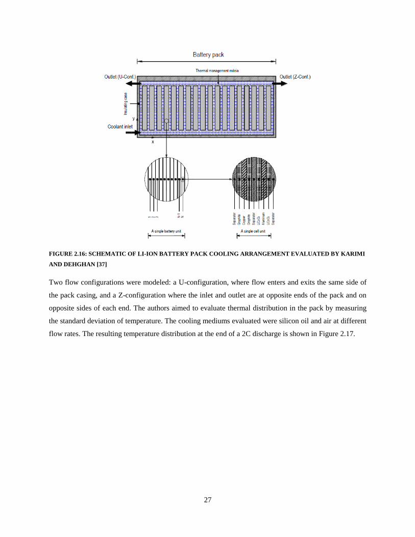
27

FIGURE 2.16: SCHEMATIC OF LI-ION BATTERY PACK COOLING ARRANGEMENT EVALUATED BY KARIMI

AND DEHGHAN [37]

Two flow configurations were modeled: a U-configuration, where flow enters and exits the same side of

the pack casing, and a Z-configuration where the inlet and outlet are at opposite ends of the pack and on

opposite sides of each end. The authors aimed to evaluate thermal distribution in the pack by measuring

the standard deviation of temperature. The cooling mediums evaluated were silicon oil and air at different

flow rates. The resulting temperature distribution at the end of a 2C discharge is shown in Figure 2.17.

28

FIGURE 2.17: TEMPERATURE DISTRIBUTIONS IN A PRISMATIC PACK FOR 4 COOLING CONDITIONS. A)

SILICON OIL, U-PATTERN, H = 100 [W/M2 K], B) AIR, Z-PATTERN, H = 250 [W/M2 K], C) SILICON OIL, Z-

PATTERN, H = 100 [W/M2 K], D) AIR, Z-PATTERN, H = 250 [W/M2 K]

Numerical results from the temperature distributions show that for both air and silicon oil, the Z-

configuration for flow results in a more uniform temperature distribution than the U-configuration.

Furthermore, silicon oil results in a much smaller temperature deviation (0.15 °C vs. 7.33 °C after 2C

discharge). The authors conclude that the penalty for improved thermal control is that parasitic power is

much higher for silicon oil, due to the high viscosity.

Researchers have investigated the use of purely passive thermal control for batteries. Thermal

management systems without blowers, fans, pumps, and piping are desirable for packaging and economic

reasons [38]. Almost all examples found in the literature are works performed with phase change

materials that undergo a change from solid to liquid as heat is absorbed by conduction from a higher

temperature region. Hence, heat absorption takes place both as sensible heat and as latent heat. When the

temperature of the battery and PCM interface reaches the melting range of the PCM, the PCM starts to

melt and the high latent heat capacity of the PCM prevents the battery temperature from rising sharply

[39].

29

Thermal conductivity and phase-change temperature of a PCM are important properties that affect the

overall performance of a thermal management system. Work has been performed to improve the thermal

conductivity of PCM by adding high conductivity structures within the material [40], or by mixing

additional high conductivity materials into the PCM [39].

Kizilel et al. [41] in their work presented a thermal management strategy for high-current applications

using PCM with expanded graphite within (PCM/EG). Their work consisted of charging and discharging

lithium-ion batteries in extreme conditions: ambient temperature of 45 °C, and discharge rates of 2.08C-

rate, while measuring surface temperatures of cylindrical cells within a pack. The authors found that high

energy packs with PCM can be discharged safely at high currents and have improved capacity

degradation rates. In Figure 2.18, the effect of PCM on a battery pack consisting of 8 series and 2 parallel

connected 18650 batteries is displayed.

FIGURE 2.18: THE EFFECT OF PCM THERMAL MANAGEMENT ON THERMAL RESPONSE OF 8S2P

BATTERY PACKS [41]

In extreme condition testing, a constant current discharge was performed on a pack with PCM at 45 °C

and a pack without PCM at 30 °C. The pack with PCM was able to release 90% of capacity before

reaching the safety shut-off, whereas the non-PCM pack at lower temperatures only reached 42%. This is

taken to demonstrate that PCM is a suitable choice for lithium-ion battery thermal control.

30

Furthermore, the authors conclude that other benefits of PCM include: compactness, reduced weight,

reduced cost and simplicity over active systems. The authors conclude that PCM passive control may

make active control, if necessary at all, complementary and/or secondary in function.

In several works, researchers perform studies to compare active and passive thermal management. In [39],

Kizilel et al. produced a comparison of active (air) and passive (PCM) cooling. A battery pack consisting

of 67 modules that each contained 20 1.5 Ah 18650 lithium batteries was modeled using a heat generation

correlation developed in a prior study as the input heat term.

In Figure 2.19, the average temperature of an interior Li-ion cell discharged under stressed conditions

(Tamb = 40 °C, discharge rate 6.67C, 50 A/module) is shown. With air-cooling, the increase in average

temperature of the cell was constant and the temperature reached approximately 60 °C at the end of the

discharge.

FIGURE 2.19: CELL TEMPERATURE INCREASE FOR PHEV-20 BATTERY PACK UNDER STRESSED

DISCHARGE CONDITIONS (TAMB = 40 °C, DISCHARGE RATE = 6.67C) [39]

The temperature profile along a single battery was studied for both the air and PCM cases. The authors

determined that the battery temperature is more uniform when PCM is used. With air-cooling, the

temperature difference along a single battery may be as high as 3 °C, and PCM-cooled batteries had in-

battery variations of less than 0.2 °C. In comparisons of side by side batteries, temperatures are also more

uniform when PCM is used. With air cooling, it was observed that as the rate of convection increases, the

temperature uniformity decreases, and thus it is concluded that air-cooling does not favor temperature

uniformity.

31

2.2.2. Experimental Works

In much of the literature, examples of empirical thermal measurements are performed merely to verify or

evaluate a numerical model. In general, numerical models dominate the literature and a lack of

experimentally focused research was noted. Especially research focused on thermal experimentation. The

empirical thermal studies found in the literature are summarized within the following subsections.

2.2.2.1. Direct Measurement

The most popular method of thermal parameter measurement is via direct measurement, which comprises

measurement via contact between a sensing element and some part of a battery or battery containment

structure. In most cases thermocouples are used, as illustrated by the following review of direct thermal

measurement studies.

The most commonly used thermal sensors are thermocouples. Many thermal models are validated on the

basis of matching temporal temperature data. An example is the electro-thermal model of Ye et al. [42].

To validate their model, the authors compared predicted battery temperatures during discharge to

measurements produced in a physical experiment. The experiment consisted of measuring the surface

temperature of a prismatic 11.5 Ah battery at a single location, the center of the battery’s largest surface.

The battery was discharged at various rates (0.2C, 0.5C, 1C, 2C) inside a temperature-controlled box with

several initial temperatures (0, 10, 25, 55 °C). Insulation was wrapped around the battery to minimize

heat transfer to the box and ambient air. The quasi-insulated state allows the assumption that all heat

generated remains within the battery, and the resulting temperature measured represents the total heat

generated during operation.

In [43], Mi et al. generated numerical and analytical thermal results for a pack consisting of 48 batteries.

To produce these results, the thermal response of an individual cell was measured with a single

thermocouple as the battery underwent discharge. The measured response was used as an input heat term

to a commercial FEA code. In the physical experiment performed, the battery was placed within a test

chamber in a vertical position with only natural convection cooling present. A single thermocouple was

used to measure the surface temperature of the battery, while another thermocouple monitored ambient

temperature. This difference between the battery and ambient temperature was used to quantify the heat

dissipation by radiation and natural convection. The study assumed a surface emissivity of 1, and

calculated natural convection cooling using known correlations. The overall heat balance used is given as

Equation (2.12), and the radiation heat transfer coefficient is given as Equation (2.13).

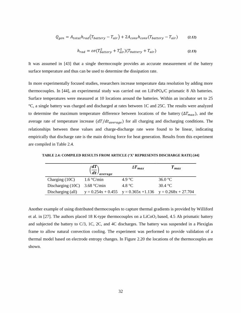
32

( ) ( ) (2.12)

(

)( ) (2.13)

It was assumed in [43] that a single thermocouple provides an accurate measurement of the battery

surface temperature and thus can be used to determine the dissipation rate.

In more experimentally focused studies, researchers increase temperature data resolution by adding more

thermocouples. In [44], an experimental study was carried out on LiFePO4/C prismatic 8 Ah batteries.

Surface temperatures were measured at 10 locations around the batteries. Within an incubator set to 25

°C, a single battery was charged and discharged at rates between 1C and 25C. The results were analyzed

to determine the maximum temperature difference between locations of the battery ( ), and the

average rate of temperature increase ( ) for all charging and discharging conditions. The

relationships between these values and charge-discharge rate were found to be linear, indicating

empirically that discharge rate is the main driving force for heat generation. Results from this experiment

are compiled in Table 2.4.

TABLE 2.4: COMPILED RESULTS FROM ARTICLE (‘X’ REPRESENTS DISCHARGE RATE) [44]

(

)

Charging (10C) 1.6 °C/min 4.9 °C 36.0 °C

Discharging (10C) 3.68 °C/min 4.8 °C 30.4 °C

Discharging (all) y = 0.254x + 0.455 y = 0.365x +1.136 y = 0.268x + 27.704

Another example of using distributed thermocouples to capture thermal gradients is provided by Williford

et al. in [27]. The authors placed 18 K-type thermocouples on a LiCoO2 based, 4.5 Ah prismatic battery

and subjected the battery to C/3, 1C, 2C, and 4C discharges. The battery was suspended in a Plexiglas

frame to allow natural convection cooling. The experiment was performed to provide validation of a

thermal model based on electrode entropy changes. In Figure 2.20 the locations of the thermocouples are

shown.

33

FIGURE 2.20: THERMOCOUPLE LOCATIONS ON A 4.8 AH PRISMATIC BATTERY USED BY WILLIFORD ET

AL. [27]

The surface temperature variation was measured during each discharge. Temperatures around the

positive, aluminum tab were found to be consistently higher (about 5 °C) than those at the negative,

copper tab. In comparing experimental and numerical model results, the authors only utilize point 14 in

Figure 2.20 in defining the battery temperature.

The effect of imposed thermal gradients on the performance of lithium-ion batteries was experimentally

investigated by Troxler et al. in [45]. A test rig was constructed to apply a thermal gradient across a

battery using liquid cooled thermoelectric elements. A schematic of the rig is shown in Figure 2.21.

FIGURE 2.21: TEST RIG WITH CELL HOLDER AND PELTIER THERMOELECTRIC ELEMENTS [45]

34

The authors performed testing on a 4.8 Ah battery. Thermal gradients ranging from 0 °C to 40 °C within

the range of -5 °C to 35 °C were generated across the battery at fixed SOC points. The results are

interpreted to determine that when thermal gradients are present across a battery the charge transfer

resistance becomes non-uniform in each cell layer of the battery. The layer units closer to the hotter side

have lower effective impedance which causes larger currents to pass through them than through the units

close to the colder side [45]. This scenario will lead to uneven heat generation within individual batteries

and is a source of safety issues highlighted in single cell [26] and pack modeling of non-uniform heat

generation [34]. It is ideal that thermal management systems minimize the thermal gradient in all

dimensions of the batteries.

Calorimetric methods have been utilized to measure heat generation as well. Kim et al. in [46] used a

three-cell isothermal micro calorimeter to investigate the dependence of thermal behavior on the

charge/discharge rate. LixMn2O4 coin cells of 2016 size (20 mm diameter, 1.6 mm high) were constructed

by the authors and placed inside wells hollowed out in a large aluminum heat sink. Thermoelectric

sensors located between the sample and the heat sink measured heat generation. The heat sink was

accurately maintained at 25 °C, while the batteries underwent C/10, C/5, C/3, and 1C discharges. The

reversible heat effect was estimated from the total heat generation rate by subtraction of irreversible heat

measured by a dc interruption technique. The authors found that the discharge rate dependence of the

thermal profile suggests that, total heat generation rate is dominated by a reversible heat effect at low and

moderate rates and by irreversible heat effects at high rates only.

In [47], Thomas and Newman performed isothermal calorimetry on 2325 size coin cells to provide

comparison and validation of a model. The test cell was encased in a copper box packed with copper shot

to fill the voids in the calorimeter and decrease the time response of the sensing element within. Heat

generation rates were measured as the cell was discharged at C/8, C/3, and 2C rates. Figure 2.22 shows

the measured heat generation profiles for C/3-rate discharges at 15, 20, 25, and 30 °C ambient

temperatures.

35

FIGURE 2.22: MEASURED HEAT GENERATION PROFILES OF LIAL0.2MN1.8O4-ΔF0.2 BASED 2325 COIN CELLS

DISCHARGED AT C/3 IN FOUR AMBIENT TEMPERATURES [47]

Lv et al. in [48] measured heat generation and temperature response of several 18650 batteries to verify a

modeling method. The batteries were initially warmed to 30 °C, then charged and discharged at 1C, 1.5C

and 2C. The temperature and temperature response ( ) were measured. Since the batteries

were discharged in an adiabatic condition, the temperature rise accounts for all the heat generated in the

cell. The authors used the energy balance in Equation (2.14), to calculate based on over-potential

and resistance values generated by the model.

(2.14)

The results were compared with experimental data and found to be highly consistent, with any small

errors accounted for by other processes not evaluated in Equation (2.14). This provides empirical

evidence that the greatest effect on heat generation and energy loss for lithium-ion batteries is total

resistance and over potential. Figure 2.23 shows the average temperature rise rates for both 1C and 2C

charges and discharges. It can be observed that the charge and discharge heating rates are approximately

mirrored when plotted against SOC. This figure is in agreement with the pattern observed by Thomas and

Newman [47] in Figure 2.22.

36

FIGURE 2.23: THE CURVE OF CHARGE-DISCHARGE HEAT RATE. (A) DISCHARGE OF 2C, (B) CHARGE OF

2C, (C) DISCHARGE OF 1C, AND (D) CHARGE OF 1C [48]

2.2.2.2. IR Thermography

As a non-invasive method of temperature measurement, infra-red (IR) thermography is an excellent tool.

In the same way that single or multiple thermocouples have been used to validate electro-thermal or

chemical models, IR images have been used as well. Niculuta and Veje in [28], utilize IR thermography

to measure the surface temperature profile of a discharging 70 Ah LiFePO4 battery. This enabled visual

determination of the spatial temperature distribution, and resulted in validation of a three-dimensional

electro-thermal model. Figure 2.24 shows the compared images.

FIGURE 2.24: IMAGES USED TO COMPARE ELECTRO THERMAL MODEL [28]

The experimental work consisted of placing the cell vertically within an environmental chamber. The

door of the chamber was replaced with a Plexiglas sheet complete with a viewport for the thermal camera

lens. The chamber was set to lab temperature to reduce error associated with lab air infiltrating through

37

the view port. In order to enable accurate temperature measurement of a surface using thermography, the

surface emissivity was required. The authors chose a value for the battery casing emissivity based on the

material type used to construct the casing. For standardized materials, the value is tabulated in literature.

For the high density poly-ethylene casing in [28], an emissivity value of 0.9 was used from a common

material specification handbook.

The authors found that with currents of 35A (C/2) or higher used to charge/discharge the cell, the

temperature profiles were not uniform. IR thermography is beneficial as it provides a method to observe

surface temperatures without affecting the properties of the surface by applying a sensor.

2.3. Summary

The literature review shows that very few studies with empirical thermal measurements of Lithium-ion

battery cells have been performed. Most works of research consist of numerical model development with

model validation from sparse experimental data. For the specific electrode chemistry (LiFePO4) that this

work is concerned with, the electrochemical operating principles are understood and have been defined in

the literature. Using electrodynamics principles, the nominal charge dynamics generated from the

movement of lithium ions is known in this chemistry is known [4].

Real world applications of Lithium-ion batteries require adequate control of operating temperature, as

battery performance and degradation have been shown to be strongly dependent on temperature [2]. This

creates a great need to characterize the heat generated by operating batteries. Electrochemical models that

attempt to do this have progressed form early 1D models [3] to 3D models [33] that couple

electrodynamics and thermodynamic processes. In this way, researchers have attempted to predict the

heat generated as a result of battery operation.

It has been shown that as heat is generated during battery operation it accumulates in the battery mass or

is dissipated by some means to an external heat sink. Modeling at the cell, or pack level demonstrates

thermal management strategies utilizing: an applied cooling coefficient (e.g. h = 0.05 W/m2K) [26]), a

modeled cooling fluid flow (air, liquid) [37]), or a mass of PCM to absorb the heat [41]. In this way, a

solution for the final temperature field can be determined and used to evaluate final average temperature,

temperature response, and/or temperature non-uniformity.

Numerical methodologies of this type depend on accurate model definition in order to achieve accurate

temperature field solutions. The temperature solution at each time step in a modeled process affects the

heat generation mechanisms that ultimately drive the changes in temperature. Experimental data are

38

required to validate model outputs and increase confidence in results. Furthermore, experimental data to

evaluate thermo-physical properties of the modeled materials are needed as well.

Existing experimental work in the literature is scarce and only a few studies that performed thermal

measurements were found. Many of such studies encompassed placing a single thermocouple to measure

temperature of a single point [42]. In [43], the temperature of the single point is assumed to represent the

surface temperature of the entire battery and forms the basis for all heat dissipation calculations.

Comparing model results to a single temperature reading is a common method of validating numerical

models.

However, multiple temperature sensing elements are required to accurately characterize heat dissipation

and evaluate the effect of temperature non-uniformity [27]. Experiments that make use of distributed

thermocouples benefit from increased surface temperature accuracy and therefore have improved heat

dissipation calculations [44].

Other methods have been utilized to investigate and characterize heat generation of operating batteries.

Calorimetric methods have been used to evaluate the heat rate due to discharges on coin cells [46], [47].

In such studies, coin cells were charged and discharged within a calorimeter and the heat generated was

sensed and measured.

Experimental works that encompass measurements of heat flux, heat generation, and temperature

distribution were not readily discovered. Since these factors directly relate to thermal management and

overall battery performed, a need exists to increase the availability of experimental thermal data and data

collection methods relating to their operation.

39

Chapter 3

Experimental Study

The experimental configurations and methodologies utilized to characterize the thermal behavior and

properties of the LiFePO4 batteries are presented in this chapter. Three different experiments were

performed in this study:

1. The first experiment consisted of direct measurements of the thermal resistance and conductivity

of the constituent battery layers and of the whole battery layer assembly. These results were

generated to provide accurate measurements for computer model programmers.

2. The second experiment measured temperature and heat flux of lithium-ion battery surfaces while

undergoing charging and discharging. The heat generated in four discharge conditions with five

different cooling conditions is determined. A special apparatus was developed to enable this

experiment.

3. The third experiment involved thermo-graphic imaging of the principal battery surface while

undergoing charging and discharging.

40

3.1. Thermal Conductivity Experiment

In this experiment, the thermal resistance and corresponding thermal conductivity of prismatic battery

materials was evaluated. The experiment was designed to measure the thermal conductivity of both the

individual electrode layers, and the overall thermal resistance of the sealed prismatic structure. The

methodology for this experiment is presented in the following sections.

3.1.1. Batteries

In this work, commercially available 20Ah LiFePO4 lithium-ion prismatic cells, shown in Figure 3.1,

were investigated. The cell specifications are given in Table 3.1.

FIGURE 3.1: COMMERCIAL 20AH LiFePO4/GRAPHITE PRISMATIC BATTERY

41

TABLE 3.1: MANUFACTURER SPECIFICATIONS OF 20AH LiFePO4 BATTERY

Specification Value Unit

Cathode Material LiFePO4 -

Anode Material Graphite -

Electrolyte Carbonate based -

Nominal Capacity ~20 Ah

Nominal Voltage 3.3 V

Nominal Energy 65 Wh

Energy Density 247 Wh/L

Mass 496 g

Discharge Power 1200 W

Dimensions 7.25 x 160 x 227 mm

Specific Power 2400 W/kg

Specific Energy 131 Wh/kg

Operating Temperature - 30 to 55 °C

Storage Temperature - 40 to 60 °C

Volume 0.263 L

Number of Cycles Min. 300, approx. 2000 Cycles

Max Discharge 300 A

Max Charge 300 A

Internal resistance 0.5 mΩ

3.1.2. Thermal Resistance Test Stand

Experimental thermal resistance measurements were made using a test apparatus designed by the

Microelectronics Heat Transfer Lab (MHTL) to measure thermal resistance properties of interface

materials. The test stand design was based on ASTM D-5470-95.

The test stand consists of two calibrated electrolytic iron heat flux meters positioned with a heater block

at the base, and a cold plate at the top. The heater block provides heat, Q, to the base of the column, while

the cold plate removes heat from the top of the column. Resistance Temperature Detectors (RTDs) are

installed along the length of the electrolytic iron components at known locations. The test column is

situated inside a bell jar capable of sustaining a vacuum when the attached pump is switched on. This

differs from the recommended apparatus design as described in ASTM D-5470. Instead of a guarded

heater to reduce the heat loss to surroundings, the vacuum and bell jar provide the same function. To

reduce losses associated with radiation, a reflective shroud is placed around the column such that the

column is fully encased, yet the shroud is not contacting the column.

A diagram of the test column apparatus is shown in Figure 3.2.

42

FIGURE 3.2: SCHEMATIC OF TEST APPARATUS

When losses to the surroundings are reduced, the heat flow in the column is assumed to be one

dimensional (1D). The uniform thermal conductivity of the iron meters provides a linear temperature

gradient along the column. The total heat flux rate through each of the heat flux meters is calculated by

(3.1):

( )

(3.1)

where ( ) is the thermal conductivity of the calibrated flux meter material, correlated with respect to

average interface temperature. is the cross-sectional area for heat transfer, and is the

temperature gradient along the column, calculated by a linear least squares fit of the temperature data. The

area for heat transfer is equivalent to the cross-sectional area of the heat flux meters (25 mm x 25 mm).

The test samples must have equal cross-sectional area to restrict 2D heat flow in the sample, and preserve

1D heat flow.

The interface material sample was placed between the two meters and a contact pressure was applied

using a linear actuator to the top of the column to minimize contact resistance. When the apparatus

43

reached steady state at the desired contact pressure and interface temperature, the temperatures of the

RTDs were recorded.

Thermal joint resistance is determined by (3.2):

(3.2)

where is the mean value for upper and lower heat flux meters and is the interpolated temperature

difference between the surfaces of the heat flux meters.

3.1.3. Procedure

Several procedures were employed to determine the thermal conductivity of the battery materials. These

procedures are presented within this section and characterize the following processes: battery dissection,

sample preparation, and thermal conductivity measurements.

3.1.3.1. Battery Sample Preparation

The battery samples used for thermal property evaluation were created from a single dissected battery.

This was required to reduce the overall size of the layered battery structure to match the geometrically

constrained apparatuses. The following procedure was used to create battery samples for testing.

3.1.3.1.1. Battery Dissection Steps

Step 1 was performed with the Experiment 2 apparatus, whereas steps 2 – 8 were performed in a fume

hood due to the toxic properties of the battery electrolyte.

1. An unused battery was discharged at C/20 rate to 0 % SOC and 0 V at room temperature.

2. The edges of the battery pouch were cut with a razor blade outside of the active layer area.

3. The electrode tabs were cut such that the active layers were released from the pouch.

4. The battery layers were removed from the pouch as one multi-layered mass.

5. The battery layers were separated and sorted into negative electrodes, positive electrode sheets

and polymer separator.

6. The materials were left untouched for several days to allow complete vaporization of the

electrolyte material.

3.1.3.1.2. Sample Preparation Steps

In Figure 3.3, the pouching material and a stack of electrode and separator layers is shown just prior to

inserting the stack of electrodes into the pouch.

44

7. The negative electrode, positive electrode and separator sheets were cut into 25 mm by 25 mm

squares to match the heat flux meter surfaces.

8. Layers of battery materials were stacked according to the sample requirements and placed

between two layers of pouch such that a pouch material layer was on the bottom and top of the

layers.

9. A pouch sealing machine was used to hermetically seal the edges of the pouch material such that

the battery layers were sealed inside.

FIGURE 3.3: IMAGE OF POUCHING MATERIAL AND STACK OF ELECTRODE LAYERS WITH SEPERATOR

LAYERS IN BETWEEN.

3.1.3.2. Thermal Conductivity Measurement Steps

10. The surfaces of the heat flux meters were cleaned with acetone to eliminate additional sources of

thermal resistance

11. A thin layer of Dow Corning 340 Thermal grease was applied to the contacting surfaces of the

heat flux meters to reduce contact resistance between the meter and sample surfaces.

12. The following parameters of the test were input to the Labview data acquisition program.

a) Mean joint temperature,

b) Contact load pressures.

c) Convergence criteria for steady-state

d) Sampling rate

13. The Labview data acquisition program was activated and controlled the operation of the

apparatus during testing. The program maintains load pressure while actively controlling heater

45

voltage to obtain steady state heat flow through the test column at the desired joint temperature

and contact pressure.

3.1.4. Test Plan

The experimental plan consisted of 8 contact pressure conditions for 8 different samples. A total of 64

measurements were taken, and repeated in two trials to reduce uncertainty. In all experiments, the joint

temperature was maintained at 40 °C, to simulate working conditions of electric vehicle batteries at

higher temperatures.

3.1.4.1. Samples

The samples used for determining thermal resistances and conductivities of the individual layers and total

battery construction are shown in Table 3.2.

TABLE 3.2: PLANNED SAMPLES FOR THERMAL CONDUCTIVITY MEASUREMENTS

Type Construction (Layering) Sample # of Layers

(N)

Negative

Electrodes

Pouch layer, separator,

N*(electrode layer, separator),

Pouch layer.

1A 25

1B 19

1C 13

1D 7

Positive Electrodes Pouch layer, separator,

N*(electrode layer, separator),

Pouch layer.

2A 25

2B 19

2C 13

2D 7

Two different sample constructions were used with four different layer-unit counts. A layer-unit is

defined in this study as 1 electrode sheet layer and one separator sheet. An additional separator layer was

included to maintain contact resistance symmetry on both the top and bottom of the samples.

3.1.4.2. Test Conditions

The thermal conductivity measurement apparatus required several input parameters to perform testing.

These parameters are displayed in Table 3.3.

46

TABLE 3.3: TEST CONDITIONS FOR THERMAL CONDUCTIVITY MEASUREMENTS

Parameter Range

Ambient Conditions vacuum (10 Pa), air

Heat Flow Rate [W] 6.3 – 9.9

Contact Pressures [MPa] 0.069 - 1.379

Mean Joint Temperature, , [°C] 38 – 42

Joint Temperature Difference [°C] 34 – 46

Sample Thickness [mm] 1.046 – 4.124

3.1.5. Analysis Method

The test rig directly outputs the thermal resistance of the samples. The resistance of individual layer units

can be interpolated from the overall sample results. The thermal resistance network of a test sample is

displayed in Figure 3.4. The resistance output from the test apparatus represents the entire resistance

network shown.

FIGURE 3.4: SIMPLIFIED THERMAL RESISTANCE NETWORK FOR BATTERY SAMPLES (HFM = ‘HEAT

FLUX METER’)

Thus, the measured overall resistance is the sum of contact resistances between the heat flux meter and

outer sample surfaces, and the resistance of the individual layers of the samples including the outer pouch

layers. To evaluate and remove the resistance associated with the outer pouch contact and pouch material,

47

the number of layer-unit in the battery sample is varied between 7 and 25 layer units. This allows a linear

regression to be performed on the data and a line of fit determined that defines the increase in thermal

resistance for an increase in sample thickness (due to increased number of internal layers). This method

also allows extrapolated to a zero layer sample where the extrapolated resistance is the contact resistance

present with all non-zero layer samples. This type of plot and the breakdown of thermal resistance values

displayed are shown in Figure 3.5.

FIGURE 3.5: BREAKDOWN OF THERMAL RESISTANCE VALUES ON RESISTANCE-THICKNESS PLOT

The fitted linear function is thus of the form given in Equation (3.3):

(

) (3.3)

The slope of Equation (3.3) is the reciprocal of the thermal conductivity-area product for the data series

that the linear function represents. The y-intercept of Equation (3.3) represents the contact resistance

between the heat flux meter and outer pouch surfaces, the bulk resistance of the pouch material, and the

48

contact resistance from the pouch surfaces to the layer-unit stack. A proportion of this resistance is due to

the properties of the pouch, but the remainder is a result of the test conditions and is not directly related or

comparable to the real world thermal performance of these interfaces. The thermal resistance of the stack

of layer-units within the pouch itself can be determined by multiplying the thickness of the layer stack by

the slope of Equation (3.3).

3.1.5.1. Thermal Conductivity Method

The output file from the TCR apparatus contains the measured thermal resistance across the interface

material. A resistance value is output for each contact pressure and temperature input. For an interface of

known thickness, the effective thermal conductivity can be determined from Equation (3.4). If the output

resistance values are used, the resulting conductivity will contain the apparent thermal conductivity of the

pouch and contact resistance.

(3.4)

By removing the contact/pouch resistance determined in Equation (3.3) from the output value, and using

the correct thickness measurement, the determined conductivity will be the effective conductivity through

a stack of layer-units. With Equation (3.5), the thermal conductivity of a layer can be evaluated with the

layer resistance determined using Equation (3.3).

(3.5)

3.2. Heat Generation and Cooling Experiment

In this experiment, a prismatic Li-ion battery was charged and discharged with thermocouples and thin-

film heat flux meters applied to the battery surfaces. In most of the tests performed, the battery was

installed inside a compression apparatus where cooling plates were directly contacting the two largest

battery surfaces. In other tests, only natural convection cooling with ambient air was present. Total heat

removed from the cell was determined along with temperature and heat flux at various locations of the

battery surface.

3.2.1. Batteries

In this experiment, the same batteries identified in Section 3.1.1 are used.

49

3.2.2. Apparatus

The test bench used for thermal characterization of the battery is shown in Figure 3.6. The components

shown in the left side of the image make up the battery cycling equipment. Whereas the components

displayed in the right of the image comprise the thermal data collection, and battery cooling system. The

compression apparatus is used to contain and insulate the battery while testing is underway with cold

plates. These major components are described in detail in the following sections.

FIGURE 3.6: CHARGE DISCHARGE TEST BENCH

50

3.2.2.1. Battery Cycling Stand

The battery cycling stand was designed and built in 2008 at the University of Waterloo to perform

component degradation studies and to enable scaled Component-In-The-Loop (CIL) testing [49]. The test

stand as a whole models a hybrid vehicle powertrain that can transfer and measure electrical energy from

an operating fuel cell, or electrical grid to 1, 2 or 3 electric vehicle batteries. A PC running a control

program in Labview is used to set and monitor charge rates, discharge rates, and battery electrical

characteristics.

The hybrid test stand was modified so that the fuel cell components were not connected to the power bus.

This enabled the test stand to behave in full EV mode, where only electric batteries are charged and

discharged using the electrical distribution grid of the lab. The voltage supply and load were a Lambda

ZUP20-40-800 and TDI Dynaload RBL232 50-150-800 respectively. Connections to the TDI Load box,

Lambda power supply and other components are shown in Figure 3.7.

A MotoTron CTRLPCM00200 controller monitored the output of battery voltage, and current sensors,

and was connected to the test stand PC via RS232 communication standard. The Labview program on the

PC recorded the values at one second intervals. Three thermocouples were connected to the MotoTron

allowing one thermocouple per cell in the original hybrid stand design. These thermocouples were

repurposed to measure lab temperature, as the thermal data collection system was implemented to record

and monitor battery temperatures (Section 3.2.2.2).

51

FIGURE 3.7: SCHEMATIC REPRESENTATION OF CHARGE DISCHARGE TEST STAND

3.2.2.2. Thermal Data Collection

The thermal data collection system is comprised of data acquisition components connected to sensors

placed on the battery surfaces.

3.2.2.2.1. Data Acquisition

All measurements were performed using a Keithley 2700 data acquisition system. A 20 channel M7700

analog input module was used to connect to output terminals of all instruments. Data logging was

programmed and controlled by a Windows based Excel add-in patch “ExcelLink” that provides

instantaneous recording of values to an Excel sheet. This software is particularly useful as the immediate

Excel format is easily used. The data acquisition hardware described is shown in Figure 3.8.

52

FIGURE 3.8: KEITHLEY 2700 DATA LOGGER AND M7700 INPUT MODULE

3.2.2.2.2. Sensors

Sensors monitored by the thermal data collection system consisted of the following types: Thermocouples

(TC) and Heat Flux Sensors (HFS). The majority of sensors were placed on the battery surfaces within the

compression rig, while the remaining sensors were installed on the battery cooling system.

Thermocouples

Thermocouples were installed on the principal surface of the battery to measure temperatures at ten

discrete points. T-type 30 gauge, special limits of error (SLE) thermocouple wire were used on one side.

The location of T-type thermocouples is listed in Table 3.4 and displayed in Figure 3.9. Kapton backed

adhesive tape (approx. 4 mm x 4 mm in size) pieces were used to adhere the thermocouples to the battery

surface.

TABLE 3.4: SPATIAL LOCATIONS OF THERMOCOUPLES (DIST. FROM BOTTOM LEFT CORNER OF

BATTERY)

Thermocouple X [mm] Y [mm]

1,1 26.5 194

1,2 78.5 194

1,3 130.5 194

2,1 26.5 169

2,2 130.5 169

3,1 26.5 130

3,2 78.5 130

3,3 130.5 130

4,1 78.5 70

5,1 78.5 35

53

FIGURE 3.9: SPATIAL ARRANGEMENT OF THERMOCOUPLES

Heat Flux Sensor (HFS).

Three thin-film heat flux sensors were installed on the surface opposite to the surface that the

thermocouples were installed upon. The locations of these three sensors are shown in Figure 3.10, and the

x and y coordinates of HFA center points is given in Table 3.5. The two sensors near the top of battery are

of the type HFS-4, which have slightly different sensitivity from the third sensor, an HFS-3. Kapton

backed adhesive tape (approx. 4 mm x 4 mm in size) pieces were used to adhere the HFS to the battery

surface.

These sensors function as a self-generating thermopile transducer. They require no special wiring,

reference junctions or signal conditioning. The HFS utilize a multi-junction thermopile construction on a

polyimide film laminate. The output of the sensors provides an average measurement of surface heat flux

in a 25.4 x 25.4 mm area (1 inch2).

13 mm

25 mm

39 mm

60 mm

35 mm

35 mm

26.5 mm

52 mm

5,1

4,1

– +

54

TABLE 3.5: SPATIAL LOCATIONS OF HEAT FLUX SENSOR CENTRE-POINTS (DIST. FROM BOTTOM LEFT

CORNER OF BATTERY)

Heat Flux Sensor Location Type of HFS X [mm] Y [mm]

1 (+) Electrode HFS-4 104.7 169.8

2 (-) Electrode HFS-4 52.3 169.8

3 Mid-surface HFS-3 78.5 122.7

FIGURE 3.10: SPATIAL LOCATIONS OF HEAT FLUX SENSOR CENTER-POINTS

3.2.2.3. Battery Cooling System

The battery cooling system consisted of a closed loop of tubing connecting two cooling plates (P1, P2) to

a Fisher Scientific Isotemp 3016 fluid bath. Sensors were placed along the flow path to record properties

of the fluid. A schematic of the system is shown in Figure 3.11. The cooling plates were placed within the

compression rig directly against the principal surfaces of the battery such that heat generated within the

battery was principally removed by conduction to the surfaces of the cooling plates.

12 mm

39.5 mm

24.5 mm

– +

55

FIGURE 3.11: SCHEMATIC OF COOLING SYSTEM FLOW FROM BATH TO COOLING PLATE (P1,P2)

INLETS/OUTLETS

3.2.2.3.1. Sensors

Two types of sensors monitored the battery cooling system: thermocouples and flow meters. These

sensors were required to determine the heat gained or lost by the fluid within the cooling plates.

Thermocouples

T-type insertion thermocouples within a thermo-well were installed directly upstream and downstream of

the inlet and outlet to each cooling plate. These thermocouples measured the bulk temperature of the fluid

flowing within the coolant line. The Keithley 2700 discussed in Section 3.2.2.2 recorded the output of

these thermocouples.

Flow meter

A Microtherm FS1 30-300ml/min flow meter was installed directly upstream of the inlet to each cooling

plate. An LCD display provides instantaneous measurement of volumetric flow. This volumetric flow

value was manually recorded at the beginning and end of test cycles.

3.2.2.3.2. Cooling Plates

A set of commercially available battery module cooling plates were selected to remove heat from the

battery within the compression rig. The cooling plates were manufactured from two stamped aluminum

plates joined in a nickel-brazing process. The cooling plate design used is shown in Figure 3.12.

Flowmeter

Flowmeter

T

T

T

T

Fluid Bath

Pump

P2 Inlet

P1 Outlet

P1 Inlet

P2 Outlet

56

FIGURE 3.12: COOLING PLATE DESIGN PROVIDED BY MANUFACTURER

The plate was characterized as having multiple flow channels with the inlets and outlets placed on the

edges of the plate, near the bottom of the battery. The coolant flow paths are symmetrical down the center

of the plate such that the flow channels were mirrored about the centerline.

For all tests de-ionized water was used as the working fluid within the battery cooling system. The

thermal properties of deionized water are displayed in Table 3.6.

TABLE 3.6: COOLING FLUID PROPERTIES

Property Value

Specific Heat [J/kg°C] 4180

Density [kg/m3] 1000

57

3.2.2.4. Compression Apparatus

A special isolating rig was created for tests that include active cooling using the battery cooling system.

The rig was created to isolate the cell from the ambient thermal environment and maintain compression of

the cooling plate/battery surface interface. In Figure 3.13, an exploded assembly of the isolating rig

without insulation is shown.

FIGURE 3.13: EXPLODED ASSEMBLY OF ISOLATING RIG BUILT FOR ACTIVE COOLING TESTS.

(INSULATION NOT SHOWN)

The compression rig is comprised of two transparent 12.7 mm thick polycarbonate sheets that the battery

and cooling plate are sandwiched between. A hole is present in each corner to allow a threaded bolt to

pass through. By tightening down the bolt fasteners, the battery is confined to the assembly by pressure.

Spacers were constructed using 9.53 mm thick polycarbonate with dimensions equal to the battery

dimensions. These spacers were required to change the distance between the cooling plate and the outer

polycarbonate plate so that the inlet, outlet and tubing would fit. For the cooling plate used in the charge

discharge tests, two spacers were used on each side, due to the design of the custom inlet/outlet

connectors used. The compression rig is shown in Figure 3.14.

58

FIGURE 3.14: COLD PLATE WITHIN COMPRESSION RIG.

3.2.3. Procedure

This procedure was followed to initiate battery cycling, and thermal data acquisition, and does not

directly describe the procedure for assembling the battery and cooling/instrumentation components within

the compression rig. As such, this procedure assumes the cell and cooling components are correctly

installed and fully connected to all other components as required.

1. The isothermal fluid bath and pump was turned on for a minimum of 3 hours prior to beginning

cycling to bring the battery, bath and compression rig to steady state temperature. The valves

leading to the plates were observed and set to open. The isothermal fluid bath was set to the

desired cooling temperature for the test. (5 °C to 35 °C)

2. The lab view code for the charge discharge stand was loaded and relevant test parameters were

input to the program. Relevant test parameters include:

a. Charge Current

b. Discharge Current

c. Number of Cycles

d. Maximum voltage at end of charge

e. Minimum voltage at end of discharge

f. Measurement sample rate

59

3. The thermal data acquisition PC and Keithley 2700 were turned on and initialized. On the PC, the

ExcelLink recording software was prepared for data acquisition. The following parameters were

set within the recording software:

a. Sample Rate

b. Measurement type per channel (temperature, or voltage)

4. The internal clocks on both PCs were synchronized to the same time to allow combining data

files.

5. The charge-discharge test stand and thermal data acquisition were then activated at the same time,

such that charging/discharging and data acquisition begin at the same instant.

6. The test continued until the desired number of battery cycles was completed.

7. Two files were created for each test.

a. Data from thermal data acquisition PC

b. Electrical charge discharge data

3.2.4. Plan

In this experiment, two different cooling methods are tested: passive natural convection, and active liquid

cooling with cooling plates. For cooling plates, four nominal coolant temperatures summarized in Table

3.7 were chosen to be implemented. These coolant temperatures are jointly considered the operating

temperatures as the procedure includes pre-cooling the batteries to the coolant temperature.

TABLE 3.7: PLANNED TESTS FOR HEAT GENERATION AND TEMPERATURE MEASUREMENT

EXPERIMENTS

Cooling Type Charge Voltage [V] Ambient/Coolant

Temperature [°C] Discharge Rates

Passive

(Ambient Air Only) 3.8 ~22 1C, 2C, 3C, 4C

Active

(Cooling Plates) 3.6

~5 1C, 2C, 3C, 4C

~15 1C, 2C, 3C, 4C

~25 1C, 2C, 3C, 4C

~35 1C, 2C, 3C, 4C

The temperature of the liquid coolant during discharges was not implemented as exactly as displayed in

Table 3.7. This is due to some heat loss in the valves and piping between the coolant reservoir and the

temperature measuring sensors at the inlets and outlets of the compression rig cooling plates. The actual

temperature of the coolant at the inlet of the cooling plates for each of the nominal planned temperatures

is listed in Table 3.8.

60

TABLE 3.8: ACTUAL COOLANT TEMPERATURES AT INLET OF COOLING PLATES

Cooling Type Nominal Coolant

Temperature [°C]

Actual Coolant

Temperature [°C]

Passive

(Ambient Air Only) Ambient 21.3 – 21.8

Active

(Cooling Plates)

5 5.6

15 15.6

25 24.5

35 33.5

3.2.4.1. Charge Profile

The charging cycle followed the pattern displayed in Figure 3.15. Charging begins when the tests are

initiated or at the end of a discharge.

FIGURE 3.15: STANDARD CHARGE PROFILE USED IN CHARGE-DISCHARGE TESTING

The discharge-cycle begins as soon as the charging completes and the battery voltage reaches the cut off

voltage.

3.2.4.2. Discharge Profile

The discharge rates given in Table 3.7Table 3.9 are constant current rates, and correspond to the values

given in Table 3.9.

0

0.5

1

1.5

2

2.5

3

3.5

4

0

5

10

15

20

25

0 3600 7200 10800 14400V

olt

ag

e (V

)

Cu

rren

t (A

)

Time (s)

Charge Current Charge Voltage Battery Voltage

61

TABLE 3.9: DISCHARGE RATES AND EQUIVALENT CURRENT

Charge/Discharge Rate Constant Current

1C 20 A

2C 40 A

3C 60 A

4C 80 A


The energy balance given in Equation (3.6) was used to determine the actual heat output of the battery. It

is assumed that all heat generated by the battery is either removed by the method of cooling or stored in

the battery. Subsections following describe the method of determining the components of (3.6).

(3.6)

3.2.1.1. Sensible Heat, ( )

The heat energy stored in the battery is termed sensible heat. It is evaluated based on the change in

temperature of the battery in conjunction with the specific heat capacity. Equation (3.7) is used to

evaluate the sensible heat energy stored in the battery when the battery temperature changes from some

initial temperature to a final temperature.

(

) (3.7)

A standard method of determining the average temperature across the entire battery surface has been

devised to enable sensible heat calculations. For each thermocouple, it is assumed that the measured

temperature represents the average of an area extending around the sensor. The areas are determined by

defining each area boundary by calculating the x and y midpoint distance between adjacent sensors.

Equation (3.8) is used to evaluate the average battery surface temperature by summing the temperature-

area products and dividing by the total area of the surface.

∑( )

(3.8)

The ten thermocouples measuring surface temperatures shown in Figure 3.9, are each assigned the areas

that correspond to their locations as shown in Figure 3.16. The physical size of the thermocouple areas is

presented in Table 3.10.

62

TABLE 3.10: X AND Y DIMENSIONS OF THERMCOUPLE AREAS

Thermocouple Area X [mm] Y [mm] Area [m2] (x10

-3)

1,1 A1,1 52.5 25.5 1.34

1,2 A1,2 52 25.5 1.33

1,3 A1,3 52.5 25.5 1.34

2,1 A2,1 78.5 32 2.51

2,2 A2,2 78.5 32 2.51

3,1 A3,1 52.5 49.5 2.60

3,2 A3,2 52 49.5 2.57

3,3 A3,3 52.5 49.5 2.60

4,1 A4,1 157 47.5 7.46

5,1 A5,1 157 52.5 8.24

FIGURE 3.16: DISTRIBUTION OF AREAS USED TO DETERMINE AVERAGE SURFACE TEMPERATURE

The rate of sensible heat accumulation is directly influenced by the battery heat generation rate and the

heat transfer coefficient out of the system. The temperature of the battery increases as heat is generated

A1,1 A1,2 A1,3

A2,1 A2,2

A3,1 A3,2 A3,3

A4,1

A5,1

x

y

63

due to the finite heat transfer coefficient to the surrounding. The rate of sensible heat accumulation is

determined from the rate of change of Equation (3.9), where is the rate that the battery temperature

changes.

(3.9)

The rate of temperature change is evaluated by measuring temperature at two times and calculating the

rate using Equation (3.10).

(

)

(3.10)

The rate of sensible heat accumulation can then be determined via Equation (3.11).

(

)

(3.11)

3.2.1.2. Heat Removed from Battery ( )

A fraction of the heat generated by the battery is removed by the cooling processes. In one series of

testing, the operating battery was placed in a vertical position and ambient air carried heat away by

natural convection. In other tests, cooling plates were present that utilized forced coolant flow to remove

heat.

3.2.1.2.1. Natural Convection Air Cooling

For a fluid at known temperature contacting a surface of known area, heat is transferred via convection

and observes Newton’s law of cooling.

( ) (3.12)

If the heat transfer coefficient and surface temperature is known, the corresponding heat transfer can be

calculated. Determining represents the fundamental challenge of thermal convection. The coefficient is

not itself a thermo-physical property of the fluid, but is dependent on numerous variables such that:

( [ ] ) (3.13)

Nusselt numbers are proportional to via the following relation:

64

(3.14)

Correlations for Nusselt numbers have been developed in experimental tests and are readily available in

mainstream heat transfer texts. These correlations correspond to specific geometries and care must be

taken when selecting the appropriate correlation to use. For buoyancy driven laminar fluid flow across a

vertical plate, the following correlation is found [50]:

( )

⁄

[ (

)

]

⁄

(3.15)

The Prandtl number, Pr is tabulated for different fluid temperature values in heat transfer texts and is

evaluated at the film temperature, which is the average temperature between the fluid and the surface to

be cooled. The Rayleigh number is calculated by the standard relation:

( ) (3.16)

3.2.1.2.2. Cooling Plates

Cooling plate heat removal rate is determined by the inlet and outlet thermocouple data, in conjunction

with the recorded flow rates. The difference in inlet and outlet temperatures is due to heat conducted from

the battery surface. The rate that heat is removed by a single cooling plate is calculated using Equation

(3.17).

( ) (3.17)

The total amount of heat energy removed by the cooling plates for a time period, can be determined

using Equation (3.18).

( ) (3.18)

The term is the average measured outlet temperature during the period , and is

determined via Equation (3.19). represents the number of temperature readings in the summation.

∑

(3.19)

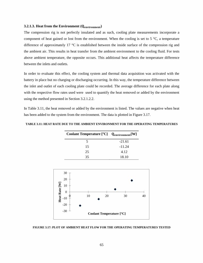
65

3.2.1.3. Heat from the Environment ( )

The compression rig is not perfectly insulated and as such, cooling plate measurements incorporate a

component of heat gained or lost from the environment. When the cooling is set to 5 °C, a temperature

difference of approximately 17 °C is established between the inside surface of the compression rig and

the ambient air. This results in heat transfer from the ambient environment to the cooling fluid. For tests

above ambient temperature, the opposite occurs. This additional heat affects the temperature difference

between the inlets and outlets.

In order to evaluate this effect, the cooling system and thermal data acquisition was activated with the

battery in place but no charging or discharging occurring. In this way, the temperature difference between

the inlet and outlet of each cooling plate could be recorded. The average difference for each plate along

with the respective flow rates used were used to quantify the heat removed or added by the environment

using the method presented in Section 3.2.1.2.2.

In Table 3.11, the heat removed or added by the environment is listed. The values are negative when heat

has been added to the system from the environment. The data is plotted in Figure 3.17.

TABLE 3.11: HEAT RATE DUE TO THE AMBIENT ENVIRONMENT FOR THE OPERATING TEMPERATURES

Coolant Temperature [°C] [W]

5 -21.61

15 -11.24

25 4.12

35 18.10

FIGURE 3.17: PLOT OF AMBIENT HEAT FLOW FOR THE OPERATING TEMPERATURES TESTED

-30

-20

-10

0

10

20

30

0 10 20 30 40

Hea

t R

ate

[W

]

Coolant Temperature [°C]

66

3.3. Thermo-graphic Experiment

In this experiment, a thermo-graphic camera was used to produces images of the principal battery surface

to visually observe temperature distribution. Using manufacturer provided software, thermal gradients are

determined.

3.3.1. Batteries

In this experiment, the same batteries identified in Section 3.1.1 are used.

3.3.2. Apparatus

A S60 FLIR ThermaCam shown in Figure 3.18 was used to produce IR images of the battery undergoing

discharge. This thermal camera has a 320 x 240 detector, standard temperature range 0 °C − 500 °C and

an accuracy of 2 % (typically 2 °C). The sensor is able to detect temperature variances as small as 0.06 °C

[51].

FIGURE 3.18: FLIR S60 THERMACAM [52]

The battery was placed on a cardboard stand constructed to hold the battery at a 45° angle relative to the

plane of the thermal detector. This arrangement eliminates the detection of radiation emitted or reflected

by the camera and operator. To eliminate reflection from the ceiling and other objects in the environment

a large cardboard box was placed over the battery and stand. The camera was positioned on a tripod

outside the enclosing box and pointed such that the detector viewed only the battery and interior of the

box. This setup is displayed in Figure 3.19.

67

FIGURE 3.19: THERMO-GRAPHIC EXPERIMENTAL SET-UP SHOWING (L) BATTERY ON STAND AND (R)

BATTERY AND CAMERA POSITIONING

In order to achieve accurate temperature measurements with the camera, the emissivity of the battery

surface was required for input to the camera software [52]. A Gier-Dunkle DB100 infra-red reflectometer

was used to measure the long wave reflectivity and emissivity of the battery surface. In Figure 3.20, the

equipment is shown.

FIGURE 3.20: PHOTOGRAPH OF GIER-DUNKLE DB100 INFRA-RED REFLECTOMETER

The reflectometer measures the total normal hemispheric reflectivity of any flat surface by measuring the

reflection of a uniform black body emitter. The instrument produces a single number; integrated

reflectance that is weighted for a room temperature black body. As such, the measured value is the total

68

hemispheric reflectivity, but also the total normal-hemispheric reflectivity due to reciprocity. The

emissivity is calculated from the reflectance using Equation (3.20).

(3.20)

3.3.3. Procedure

The experiment consisted of two phases: determining battery surface emissivity, and recording of IR

images of a discharging battery.

3.3.3.1. Emissivity Determination

1. The DB100 was switched on and allowed to warm up for 1 hour prior to proceeding.

2. Calibration was performed on the equipment using a metallic disk with a known surface

emissivity on each side. (Gold: 0.953/Black: 0.094). With the black side placed over the sample

port, the “zero” was adjusted until 0.094 is obtained. The disk was then flipped over and the gain

was adjusted until the proper 0.953 value is obtained.

3. The battery surface was placed over the sample port. The reflectivity of the surface was output on

the digital readout and recorded manually.

3.3.3.2. Discharging

1. The battery was placed in the stand built to hold the battery at 45°.

2. The isolating box was placed over the battery and stand.

3. The positive and negative leads were connected to the battery electrode tabs. The leads entered

the box through an access hole.

4. Charging was performed on the battery until the battery reached a fully charged state.

5. When the battery was fully charged, the camera was oriented in a level position and pointed such

that it viewed only the interior of the box and the surface of the battery. Settings in the camera

were prepared to record images at 20 second intervals once underway.

6. Discharge current rate was modified in the battery cycling stand computer, and the internal clocks

on the camera and computer were synchronized. The battery discharge and camera recording

were then activated simultaneously.

7. At the end of discharge, the battery was recharged, and the images were removed from the

camera to create space in the memory for following tests.

3.3.4. Plan

In this experiment, three constant current discharge rates were used. The discharge rates used were 4C,

3C, and 2C. The charge profile used was the same as in Section 3.2.4.1.

69


The temperature readings taken by the thermal camera are included in the file header of the output image

files. Since the camera has a 320 x 240 detector, the data is in the form of a 320 x 240 numerical matrix.

The software provided by FLIR allows output of this data to .CSV format, which can then be imported

into Excel for analysis. Temperature data from the collected images for each test were input to Excel and

analyzed to determine: the temperature response along three separate lines traversing the battery surface,

the evolution of temperature gradient along those lines, and the average temperature response (

) and thermal gradient ( ) for the discharges. The locations of the three lines

representing the thermal gradients evaluated are shown in Figure 3.21. The line displayed on the right side

of the image corresponds to the negative electrode side (anode during discharge), whereas the line on the

left side corresponds to the positive electrode (cathode during discharge). A middle line is evaluated as

well.

FIGURE 3.21: LINE LOCATIONS WHERE THERMAL GRADIENT DATA WAS EVALUATED FROM IR IMAGES

Using the FLIR software in conjunction with image editing software, the pixels corresponding to the

gradient lines were used to determine the exact row and columns of the output .CSV files that are the

temperature readings along the respective lines. These temperatures were then collected from each image

taken and consolidated to a single Excel file.

Cathode

(+)

Anode

(-)

70

3.3.5.1. Temperature Response

The temperature response is a measure of the change in temperature during a period of time. In this

experiment, results are determined in [°C/s]. The response of a specific point along any of the projected

lines of the battery at time is evaluated using Equation (3.21). The change in temperature measurements

divided by the time difference between readings gives the average temperature response during the two

times selected. In general the rate of change of temperature is representative of sensible heat accumulation

in the area/volume evaluated. When comparing ( ) of two different locations of equal material

properties, higher ( ) values indicate higher heat accumulation or generation rates.

(

)

(

) (3.21)

Equation (3.22) is used to determine the average temperature response along the entire line at time . The

divisor of (3.22) represents the number of readings along the line, which corresponds to the number of

pixels encompassing the line in the image of Figure 3.21. The result of this equation for each thermal

image taken during a discharge is required for input to Equation (3.23).

(

)

∑(

)

(3.22)

The average temperature response along a line for the entire discharge process can be evaluated by

summing the individual averages for each time period and dividing by the number of measurements

during the discharge, as in Equation (3.23). By determining the average temperature response rate for

evaluated lines during the entire discharge process, the effect of discharge rate on temperature response

rate can be evaluated.

(

)

(

)

(

)

(3.23)

3.3.5.2. Thermal Gradient

The thermal gradient on the battery surface is a measure of the change in temperature per unit distance.

Results are determined in [°C/mm]. The thermal gradient at time between two points, and is

determined by Equation (3.24). The divisor of (3.24) represents the distance between the two points

where the thermal gradient is evaluated. In general, the temperature gradient is a measure of temperature

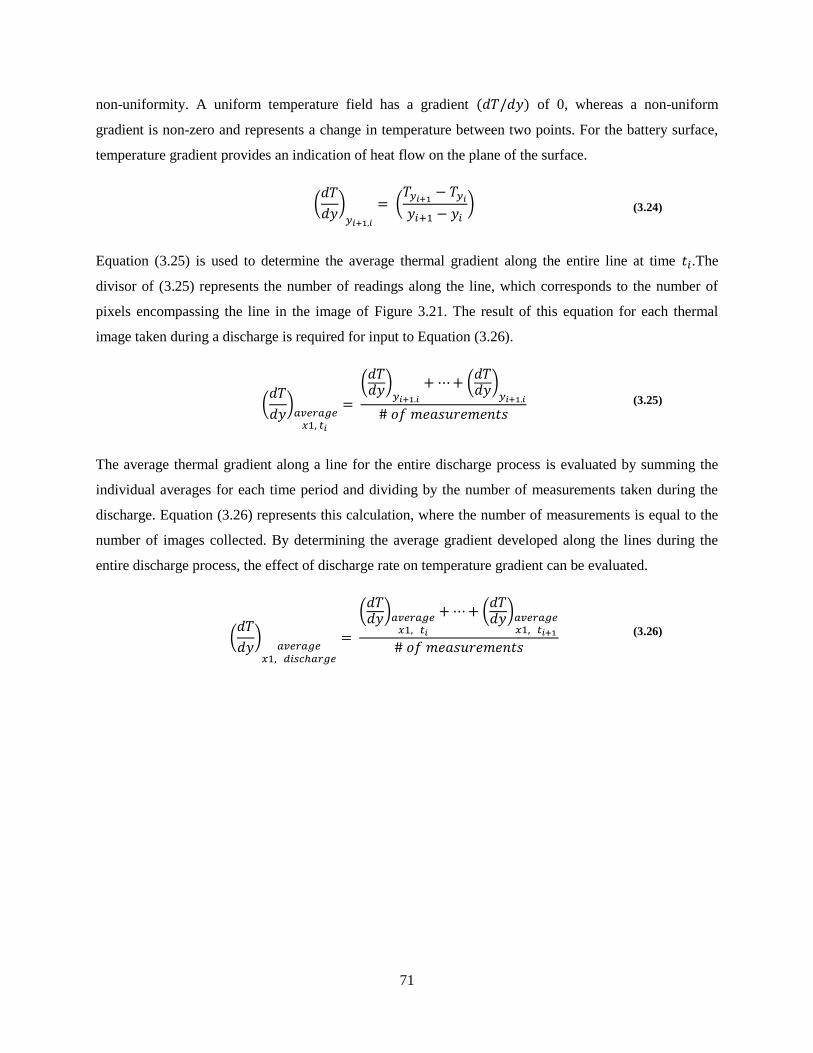
71

non-uniformity. A uniform temperature field has a gradient ( ) of 0, whereas a non-uniform

gradient is non-zero and represents a change in temperature between two points. For the battery surface,

temperature gradient provides an indication of heat flow on the plane of the surface.

(

)

(

) (3.24)

Equation (3.25) is used to determine the average thermal gradient along the entire line at time .The

divisor of (3.25) represents the number of readings along the line, which corresponds to the number of

pixels encompassing the line in the image of Figure 3.21. The result of this equation for each thermal

image taken during a discharge is required for input to Equation (3.26).

(

)

(

)

(

)

(3.25)

The average thermal gradient along a line for the entire discharge process is evaluated by summing the

individual averages for each time period and dividing by the number of measurements taken during the

discharge. Equation (3.26) represents this calculation, where the number of measurements is equal to the

number of images collected. By determining the average gradient developed along the lines during the

entire discharge process, the effect of discharge rate on temperature gradient can be evaluated.

(

)

(

)

(

)

(3.26)

72

Chapter 4

Experimental Results and Discussion

The results generated from the analysis are presented within this section, and have been organized by

experiment in the same format as the preceding chapter.

73

4.1. Thermal Conductivity Results

The experimental data collected was analyzed to produce the following thermal property results. An

evaluation of the uncertainty associated with the following results is available in Appendix A, while the

complete data generated in testing is supplied in Appendix B.

4.1.1. Thermal Resistance

The thermal resistance of samples was output directly by the apparatus, using the method outlined in

Section 3.1.2. Individual layer resistances were determined using the method outlined in Section 3.1.5.1.

Eight load conditions were placed on each sample and the resulting thermal resistances were recorded.

For each sample the testing was repeated three times and the average of the measurements are used for

analysis. These values are displayed in Figure 4.1.

FIGURE 4.1: ALL THERMAL RESISTANCES MEASURED

The 1.38 MPa (200 PSI) load condition measurements contain the smallest component of contact

resistances and thus are used to determine the resistance of individual layer-units within the samples. The

relative uncertainty in thermal resistance measurements determined in Appendix A is 10 %.

0

1

2

3

4

5

6

7

8

9

10

0 0.2 0.4 0.6 0.8 1 1.2 1.4 1.6

Th

erm

al

Res

ista

nce

[K

/W]

Load Pressure [MPa]

Neg. 7 Layer Units Neg. 13 Layer Units

Neg. 19 Layer Units Neg. 25 Layer Units

Pos. 7 Layer Units Pos. 13 Layers Units

Pos. 19 Layers Units Pos. 25 Layers Units

74

4.1.1.1. Positive Electrode Samples (Cathodes)

In Figure 4.2, the four average thermal resistances of the positive electrode samples measured at 1.38

MPa (200 PSI) are plotted against the sample thicknesses.

FIGURE 4.2: POSITIVE ELECTRODE SAMPLE AVERAGE THERMAL RESISTANCES AT 1.38 MPA LOAD

PRESSURE

In Table 4.1, the average thermal resistances determined for the positive electrode samples are listed.

These values make up Figure 4.2, and the thermal resistance values are for the complete sample cross

section, including the outer pouch layers and inner layer-units.

TABLE 4.1: THERMAL RESISTANCES OF POSITIVE ELECTRODE SAMPLES WITH 1.38 MPA LOAD

CONDITION

Sample Thermal Resistance [°C/W]

Positive 7 Layer 4.102




The thermal resistance values of positive electrode samples increase as the number of layer-units within

the test samples increase. This is as expected since increasing the number of layers increases the overall

length or thickness of the sample that heat must conduct through.

7 Layer

13 Layer

19 Layer

25 Layer

y = 0.8617x + 3.058

R² = 0.9963

0

1

2

3

4

5

6

7

0 0.5 1 1.5 2 2.5 3 3.5 4 4.5

Th

erm

al

Res

ista

nce

[°C

/W]

Thickness [mm]

75

4.1.1.2. Negative Electrode Samples (Anodes)

In Figure 4.3, the four average thermal resistances of negative electrode samples measured at 1.38 MPa

(200 PSI) are plotted against the number of layer-units.

FIGURE 4.3: NEGATIVE ELECTRODE SAMPLE AVERAGE THERMAL RESISTANCES AT 1.38 MPA LOAD

PRESSURE.

In Table 4.2, the average thermal resistances determined for the negative electrode samples are listed.

These values make up Figure 4.3. These thermal resistance values are for the complete sample cross

section, including the outer pouch layers and inner layer-units.

TABLE 4.2: THERMAL RESISTANCES OF NEGATIVE ELECTRODE SAMPLES WITH 1.38 MPA LOAD

CONDITION

Sample Thermal Resistance [°C/W]

Negative 7 Layer 3.104




The thermal resistance values of negative electrode samples increase as the number of layer-units within

the test samples increase. This is as expected since increasing the number of layers increases the overall

length or thickness of the sample that heat must conduct through.

7 Layer

13 Layer

19 Layer

25 Layer

y = 1.3252x + 2.2627

R² = 0.99

0

1

2

3

4

5

6

7

0 0.5 1 1.5 2 2.5 3

Th

erm

al

Res

ista

nce

[°C

/W]

Thickness [mm]

76

4.1.1.3. Individual Layer Unit Resistances

In Excel, a linear regression was performed on the positive electrode sample data displayed in Figure 4.2.

The determined expression is Equation (4.1):

( ) (4.1)

The slope of Equation (4.1) is 0.8617 and is equivalent to (1/kA). The thermal resistance of a positive

electrode material of equivalent type can be determined by multiplying the thickness of the sample in

question with the slope of Equation (4.1). For the positive electrode layer-units considered in this study,

the thermal resistance was found to be 0.1387 °C/W.

A linear regression was also performed for the negative electrode sample data displayed in Figure 4.3.

The determined expression is Equation (4.2).

( ) (4.2)

The slope of Equation (4.2) is 1.3252 and is equivalent to (1/kA). The thermal resistance of a negative

electrode material of equivalent type can be determined by multiplying the thickness of the sample in

question with the slope of Equation (4.2). For the negative electrode layer-units considered in this study,

the thermal resistance was found to be 0.1564 °C/W.

The Y-intercept of Equation (4.1) and (4.2) represents the thermal resistance of the contact between the

outer pouch material and the bulk resistance through the pouch material as well. This additional resistance

is an artifact of the test methods and apparatus and does not necessarily represent the contact resistance

present in battery pack applications.

In Table 4.3, the coefficients of the determined linear equations have been summarized along with the

determined thermal resistances for individual layer-units. The uncertainty in thermal resistance of a layer

unit was determined to be 10% in Appendix C, while the absolute error for each layer-unit resistance is

tabulated in Table 4.3.

TABLE 4.3: LAYER-UNIT RESISTANCE SUMMARY

Layer-Unit Type Slope

[°C/Wm]

Resistance

Associated with

Sample Pouch

[°C/W]

Thickness

(x 103) [m]

Thermal

Resistance

[°C/W]

±

[°C/W]

Positive Electrode 0.8617 3.058 0.161 0.1387 10 % 0.0139

Negative Electrode 1.3252 2.263 0.118 0.1564 10 % 0.0156

77

4.1.2. Effective Thermal Conductivity of Samples

The effective thermal conductivity was determined using the method described in Section 3.1.5.1.

Effective thermal conductivity refers to the overall conductivity determined across a cross section of

interest. By removing the component of the thermal resistance measured that represents contact resistance

and the outer pouch material, the thermal resistance of the actual stacks of layer-units can be determined

and used to find the effective thermal conductivity of those layer stacks when the thickness of the stacks

is known.

4.1.2.1. Thicknesses of Battery Materials and Samples

The thickness of all samples tested and the materials samples are composed of was measured using the

laser micrometer. Since the 1.38 MPa (200 PSI) condition is used for determining the thermal

conductivity, the thickness measurements were also made when samples had a 1.38 MPa applied load. In

Table 4.4, the thicknesses are summarized.

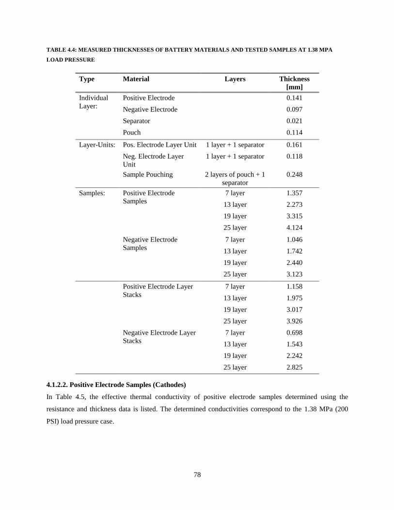
78

TABLE 4.4: MEASURED THICKNESSES OF BATTERY MATERIALS AND TESTED SAMPLES AT 1.38 MPA

LOAD PRESSURE

Type Material Layers Thickness

[mm]

Individual

Layer:

Positive Electrode 0.141

Negative Electrode 0.097

Separator 0.021

Pouch 0.114

Layer-Units: Pos. Electrode Layer Unit 1 layer + 1 separator 0.161

Neg. Electrode Layer

Unit

1 layer + 1 separator 0.118

Sample Pouching 2 layers of pouch + 1

separator

0.248

Samples: Positive Electrode

Samples

7 layer 1.357

13 layer 2.273

19 layer 3.315

25 layer 4.124

Negative Electrode

Samples

7 layer 1.046

13 layer 1.742

19 layer 2.440

25 layer 3.123

Positive Electrode Layer

Stacks

7 layer 1.158

13 layer 1.975

19 layer 3.017

25 layer 3.926

Negative Electrode Layer

Stacks

7 layer 0.698

13 layer 1.543

19 layer 2.242

25 layer 2.825

4.1.2.2. Positive Electrode Samples (Cathodes)

In Table 4.5, the effective thermal conductivity of positive electrode samples determined using the

resistance and thickness data is listed. The determined conductivities correspond to the 1.38 MPa (200

PSI) load pressure case.

79

TABLE 4.5: MEASURED THICKNESSES OF POSITIVE ELECTRODE SAMPLES AT 1.38 MPA LOAD

Sample Layer-Unit Stack

Resistance [°C/W]

Thermal Conductivity

[W/m°C] (@1.38 MPa)

Positive (7) 1.020 1.720

Positive (13) 1.647 1.832

Positive (19) 2.500 1.853

Positive (25) 3.418 1.768

4.1.2.3. Negative Electrode Samples (Anodes)

In Table 4.6, the effective thermal conductivity of negative electrode samples determined using the

resistance and thickness data is listed. The determined conductivities correspond to the 1.38 MPa (200

PSI) load pressure case.

TABLE 4.6: MEASURED THICKNESSES OF NEGATIVE ELECTRODE SAMPLES AT 1.38 MPA LOAD

Sample Layer-Unit Stack

Resistance [°C/W]

Thermal Conductivity

[W/m°C] (@1.38 MPa)

Negative (7) 0.901 1.287

Negative (13) 2.189 1.124

Negative (19) 3.156 1.123

Negative (25) 3.680 1.210

4.1.2.4. Individual Layer Unit Conductivities

The individual layer-unit thermal conductivities were determined using the values for individual layer-

unit thermal resistance in conjunction with thickness. A layer-unit is one electrode layer and one separator

layer stacked together. As such, the thermal properties include the contact resistance between the

electrode and separator sheets. In Table 4.7, the calculated thermal conductivity at 1.36 MPa is listed

with thermal resistance values and absolute and relative uncertainty values from Appendix A.

The positive electrode thermal conductivity was found to be 1.80 W/m°C, which is higher than the values

used for modeling in works found in the literature [24], [26]. The negative electrode thermal conductivity

was found to be 1.17 W/m°C which is also higher than the literature reported values.

TABLE 4.7: DETERMINED THERMAL RESISTANCE AND CONDUCTIVITY OF INDIVIDUAL LAYER-UNITS

Layer-Unit Type Thermal

Resistance [°C/W]

Thermal

Conductivity

[W/m°C]

±

[W/m°C]

Positive Electrode 0.1387 1.799 10 % 0.180

Negative Electrode 0.1564 1.170 10 % 0.117

80

4.2. Heat Generation and Cooling Results

The data produced in the heat generation and cooling requirements experiment consists of electrical data

(battery voltage, and current flow) as well as thermal data: surface temperature data (13 channels), heat

flux meter output voltages (3 channels), inlet/outlet cooling system temperatures (4 channels). In order to

manipulate the large spread sheets of data, MATLAB software was used. An evaluation of the uncertainty

associated with the following results is available in Appendix A.

4.2.1. Effect of Discharge Rate and Operating Temperature on Battery Temperature

The temperature of the ten points measured on the battery surface has been plotted against time for each

discharge in Appendix C.

4.2.1.1. Surface Temperature Response

The surface temperature response is the change in surface temperatures at specific locations over the

course of a discharge. In Figure 4.4, the temperature values recorded by the ten surface thermocouples are

plotted as a function of depth of discharge for the 1C, 15 °C coolant case. It can be observed that the

response of the thermocouple at location 1,1 has the faster rate of increase between 0.0 and 0.2 depth of

discharge (DOD). This thermocouple is nearest the negative electrode of the battery and indicates the

location of highest heat accumulation. The response curves all appear to become constant, such that no

temperatures increase greatly between 0.2 and 0.6 DOD. This represents a period where the heat

generation and cooling were nearly equivalent. After 0.8 DOD the temperatures begin to increase at rates

greater than the initial period.

81

FIGURE 4.4: TEMPERATURE RESPONSE AT EACH THERMOCOUPLE DURING 1C DISCHARGE AT 15 °C

OPERATING TEMPERATURE

In Figure 4.5, the temperature values recorded by the ten surface thermocouples are plotted as a function

of depth of discharge. This particular case is for a 4C discharge at the same coolant/operating temperature

(15 °C) as the previous figure. By comparing between images, the difference in response to increased

current draw and thus current density can be seen. The (1,1), (1,2) and (1,3) thermocouples have

approximately equivalent rates of increase over the entire period. This indicates that the accumulation of

heat, and likely the rates of heat generation are highest near the electrodes.

Furthermore, unlike the 1C case, the is no period where the battery temperatures appeared constant,

indicating that the 4C discharge rates produce heat at a rate greater than the cooling potential provided by

the plates at the tested flow rates.

14

15

16

17

18

19

20

21

0 0.1 0.2 0.3 0.4 0.5 0.6 0.7 0.8 0.9 1

Tem

per

atu

re [

°C]

Depth of Discharge

1,1 1,2 1,3 2,1 2,2

3,1 3,2 3,3 4,1 5,1

82



In Figure 4.6, the temperature values recorded in a 4C discharge at coolant/operating temperature of 35

°C by the ten surface thermocouples are plotted as a function of depth of discharge.



14

16

18

20

22

24

26

28

30

0 0.1 0.2 0.3 0.4 0.5 0.6 0.7 0.8 0.9 1

Tem

pea

rtu

re [

°C]

Depth of Discharge

1,1 1,2 1,3 2,1 2,2

3,1 3,2 3,3 4,1 5,1

30

32

34

36

38

40

42

44

46

0 0.1 0.2 0.3 0.4 0.5 0.6 0.7 0.8 0.9 1

Tem

per

atu

re [

°C]

Depth of Discharge

1,1 1,2 1,3 2,1

2,2 3,1 3,2 3,3

4,1 5,1

83

4.2.1.2. Average Temperature

In Figure 4.7, the maximum average surface temperatures of the battery for the four discharge rates and

operating/cooling temperatures has been plotted. The trend shows that regardless of operating temperature

the maximum average surface temperature increases as the rate of discharge is increased. In Table 4.8,

the maximum average surface temperatures are summarized for the test conditions used.

FIGURE 4.7: MAXIMUM AVERAGE SURFACE TEMPERATURES OF BATTERY FOR ALL DISCHARGE RATES

AND COOLANT/OPERATING TEMPERATURES TESTED

TABLE 4.8: SUMMARY OF MAXIMUM AVERAGE SURFACE TEMPERATURES OF BATTERY FOR ALL

DISCHARGE RATES AND COOLANT/OPERATING TEMPERATURES TESTED

Cooling Type Operating/Coolant

Temperature [°C]

Maximum Temperature [°C]

1C 2C 3C 4C

Passive

(Ambient Air Only) ~22 30.5 36.5 41.2 45.4

Active

(Cooling Plates)

5 10.1 13.3 15.7 18.9

15 19.6 22.9 25.4 28.0

25 27.6 30.4 32.6 35.2

35 35.9 38.2 40.3 42.3

Since the increase in coolant/operating temperature can account for much of the differences in Figure 4.7,

it is useful to consider the difference between the start of discharge average surface temperature and the

0

5

10

15

20

25

30

35

40

45

50

0 1 2 3 4 5

Tem

per

atu

re [

°C]

Discharge Rate [C]

5 °C Water 15 °C Water


22 °C Air

84

end of discharge average surface temperature. This provides a measure of the buildup of heat within the

battery. In Figure 4.8, the differences are plotted.

FIGURE 4.8: DIFFERENCE IN AVERAGE SURFACE TEMPERATURE BETWEEN START AND END OF

DISCHARGES

0

5

10

15

20

25

30

0 1 2 3 4 5

Tem

per

atu

re I

ncr

ea

se [

°C]

Discharge Rate [C]



22 °C Air

85

4.2.2. Effect of Discharge Rate and Operating Temperature on Heat Generation

Figure 4.9 shows the measured heat generation rates of the battery for all 1C, 2C, 3C and 4C discharge

rates at 25 °C as a function of depth of discharge (DOD: varying from 0 to 1). It can be seen that after a

steep rise in the first 0.04 of discharge, the heat generation rate becomes approximately constant until 0.5

DOD when a steady increase is observed. The increase appears to become steeper as the discharge

progresses and is highest just before the end of discharge (>0.97 DOD). Furthermore, it can be seen that

the increase in discharge rate and thus discharge current causes consistent increase in the heat generation

rate for equal depth of discharge points.

The increased heat generation can be accounted for by looking at Equation (2.3) and (2.4) in Section 2.2.

As the current is increased with the discharge rate, the irreversible ohmic heating term becomes larger.

From Equation (2.5), the current collector heat generation increases with the square of current. From this

it follows that more heat will be generated at higher discharge rates. In Table 4.9 the maximum heat

generation rates that the battery discharges with liquid cooling plates produced are tabulated.

FIGURE 4.9: HEAT GENERATION RATES OF LIFEPO4 BATTERY FOR FOUR DISCHARGE RATES AT 25 °C

-10

0

10

20

30

40

50

60

70

80

90

0 0.1 0.2 0.3 0.4 0.5 0.6 0.7 0.8 0.9 1

Hea

t G

enea

rtio

n R

ate

[W

]

Depth of Discharge

1C - 25°C

2C - 25°C

3C - 25°C

4C - 25°C

86

TABLE 4.9: SUMMARY OF MAXIMUM HEAT GENERATION RATES FOR FOUR DISCHARGE RATES AT FOUR

OPERATING TEMPERATURES

Cooling Type Charge Voltage [V] Operating/Coolant

Temperature [°C]

Peak Heat Rate [W]

1C 2C 3C 4C

Active


5 24.0 50.4 68.3 90.7

15 22.5 44.2 73.8 88.7

25 19.4 36.9 56.2 82.3

35 12.5 29.5 38.7 48.5

4.2.2.1. Total Heat Generated

Figure 4.10 shows the total heat generated in the battery discharges determined using the energy balance

presented as Equation (3.6) in Section 3.2.1. In general, the trend shows that increased discharge rate and

decreased temperatures result in increased amount of heat produced during a discharge. This follows from

the results in Figure 4.9 that show that for an equal operating temperature, higher discharges produce

higher instantaneous heat generation rates at equivalent depth of discharge. Thus for a full discharge, the

total heat generated is also always larger.

FIGURE 4.10: TOTAL HEAT PRODUCED FOR EACH DISCHARGE CONDITION AND COOLING CONDITION

In Table 4.10, a summary of the total heat generation values for the discharges and operating temperatures

is provided. The highest value of heat produced was found to be 41.34 kJ when the operating/coolant

0

5

10

15

20

25

30

35

40

45

0 1 2 3 4 5

To

tal

Hea

t [K

J]

Discharge Rate [C]

22 °C Passive 5 °C Active

15 °C Active 25 °C Active

35 °C Active

87

temperature was at 5 °C and the discharge rate 4C. This is almost twice the heat generated by the

equivalent discharge at 35 °C (an increase of approx. 30 °C).

TABLE 4.10: SUMMARY OF TOTAL HEAT PRODUCED FOR EACH DISCHARGE CONDITION AND COOLING

CONDITION


Temperature [°C]

Heat Generated per Discharge [kJ]

1C 2C 3C 4C

Passive

(Ambient Air Only) 3.8 V ~22 13.34 21.52 28.41 33.35

Active


5 27.76 34.31 38.74 41.34

15 19.59 25.59 31.27 35.44

25 11.54 18.20 22.88 26.70

35 8.09 14.28 18.58 21.25

An analysis of uncertainty (Appendix A) determined the uncertainty in total heat generation values is

strongly influenced by the range of average surface temperatures measured during a discharge. In

Appendix A, Section A.3.3, the uncertainty is listed for each operating/cooling temperature. The 5 °C

operating temperature tests resulted in the highest values of uncertainty, at 44.9%. The relative

uncertainty decreased in higher temperature tests to minimums of 34.5% with cooling plates and 24.5%

with 22 °C natural convection cooling tests. The large difference in uncertainty between the cooling plate

tests and natural convection tests is due to the absence of flow meter uncertainty when only natural

convection accounted for cooling. The flow rate uncertainty is the largest factor in the cooling plate heat

calculations and greatly affects the overall uncertainty of heat generation calculations when cooling plates

are utilized.

88

4.2.2.2. Surface Heat Flux Sensors

The surface heat flux meters were placed as described in Section 3.2.2.2.2. To refresh the reader, HFS 1 is

located near the positive electrode along the top of the battery surface, and HFS 2 is similarly near the

negative electrode. HFS 3 is located at about the middle of the battery surface.

4.2.2.2.1. Discharge Response

In Figure 4.11, the response of the heat flux meters for two discharge rates, 1C and 4C at 5 °C

operating/coolant temperatures is plotted as a function of depth of discharge. In the figure, dashed lines

correspond to 1C, while solid lines correspond to 4C. These two cases were chosen for inclusion in this

section as 5 °C tests have the highest heat generation rates.

FIGURE 4.11: HEAT FLUX SENSOR RESPONSE DURING 1C AND 4C DISCHARGE AT 5 °C OPERATING

TEMPERATURE.

From Figure 4.11, it can be observed that the 4C case has higher instantaneous heat flux values at all

times when comparing the same sensor. In general, HFS 1 and 2 measured much larger values, but are

within the same order of magnitude as the output from HFS 3. This indicates that the location of higher

heat generation is near the electrodes. When comparing between HFS 1 and 2, the result is not as clear.

The 4C case illustrates that HFS 1, nearest the positive electrode, measures higher heat flux values when

DOD is less than 0.6. From DOD = 0.6 to the end of discharge, HFS 2 measured higher values of heat

flux. The 1C case shows very little variation between HFS 1 and 2 throughout discharge. At the end of

discharge HFS 2 is reading a slightly higher heat flux as well.

0

1000

2000

3000

4000

5000

6000

0 0.2 0.4 0.6 0.8 1

Hea

t F

lux [

W/m

2]

Depth of Discharge

HFS 1

HFS 2

HFS 3

HFS 1

HFS 2

HFS 3

4C

1C

4C

1C

89

All of the heat flux sensor response curves appear to visually match the heat generation rate profiles

provided in Section 4.2.2, and Appendix C

4.2.2.2.2. Average Heat Fluxes

In Figure 4.12 the average heat fluxes measured by the three heat flux sensors for all operating

temperatures are plotted against discharge rate. It is observed that the highest average heat fluxes were

measured at HFS 1 and HFS 2 when 5 °C cooling was used and 4C discharge rates were used. In general,

for all tests the sensors nearest the electrodes (HFS 1 and 2) measured heat fluxes higher than the sensor

located at the middle of the battery surface. The trend observed is that increased discharge rates and

decreased operating temperature results in increased average heat fluxes at the three locations measured.

FIGURE 4.12: EFFECT OF INCREASED DISCHARGE RATE ON AVERAGE HEAT FLUX [W/M2] MEASURED AT

3 DIFFERENT LOCATIONS FOR ALL OPERATING TEMPERATURES

In Table 4.11, the values of Figure 4.12 are tabulated along with the average heat fluxes for the passive

cooling natural convection cases. For the passive cases, the average heat flux of HFS 2, near the negative

electrode is always highest. Liquid cooling cases do not show a definitive pattern between HFS 1 and 2.

This is likely due to the slightly uneven cooling gradient across the utilized cooling plate. The coolant

temperature and thus plate temperature increases across the width of the battery surface as heat is

absorbed. This is in contrast to the passive cooling case, where the vertical orientation of the battery

provided a condition where cooling potential is approximately equal across the width of the surface. It

0

500

1000

1500

2000

2500

3000

3500

0 1 2 3 4 5

Av

era

ge

Hea

t F

lux [

W/m

2]

Discharge Rate [C]

5 °C HFS 1 5 °C HFS 2 5 °C HFS 3

15 °C HFS 1 15 °C HFS 2 15 °C HFS 3

25 °C HFS 1 25 °C HFS 3 25 °C HFS 3

35 °C HFS 1 35 °C HFS 3 35 °C HFS 3

90

could be inferred that the passive cooling cases are a better representation of the differences in heat

generation between the three locations.

TABLE 4.11: SUMMARY OF AVERAGE HEAT FLUX MEASURED AT 3 LOCATIONS FOR ALL OPERATING

TEMPERATURES

Cooling

Type

Charge

Voltage [V]

Operating/Coolant

Temperature [°C]

Average Heat Flux [W/m2]

Position 1C 2C 3C 4C

Passive

(Ambient Air

Only

3.8 ~22

1 42.3 130.3 238.4 343.6

2 46.3 145.7 239.6 373.4

3 24.6 71.1 108.6 145.3

Active

(Cooling

Plates)

3.6

5

1 575.5 1294.5 2347.7 3112.2

2 599.3 1390.8 2259.5 3072.8

3 149.4 341.3 539.3 764.1

15

1 475.7 1029.7 1711.8 2419.0

2 781.4 1509.9 2351.6 2887.1

3 157.9 331.7 548.4 697.3

25

1 148.2 684.9 1597.3 2309.3

2 168.9 733.2 1851.6 2648.2

3 74.4 194.8 413.0 611.1

35

1 47.6 585.6 1468.4 2160.2

2 86.1 689.7 1579.9 2101.5

3 25.2 163.3 340.6 471.8

4.2.2.2.3. Peak Heat Flux

In Figure 4.13, the peak heat fluxes measured by the three heat flux sensors for all operating temperatures

are plotted against discharge rate. It is observed that the highest peak heat fluxes were always measured at

HFS 2. In general, for all tests the sensors nearest the electrodes (HFS 1 and 2) measured greater peak

heat fluxes than the sensor located at the middle of the battery surface. The trend observed is that

increased discharge rates and decreased operating temperature results in increased peak heat fluxes at the

three locations measured.

In Table 4.12, the values of Figure 4.13 are tabulated along with the average heat fluxes for the passive

cooling natural convection cases.

91

FIGURE 4.13: EFFECT OF INCREASED DISCHARGE RATE ON PEAK HEAT FLUX [W/M2] MEASURED AT 3

DIFFERENT LOCATIONS ALL OPERATING TEMPERATURES

TABLE 4.12: SUMMARY OF PEAK HEAT FLUX MEASURED AT 3 LOCATIONS FOR ALL OPERATING

TEMPERATURES

Cooling

Type

Charge

Voltage [V]

Operating/Coolant

Temperature [°C]

Peak Heat Flux [W/m2]

Position 1C 2C 3C 4C

Passive

(Ambient Air

Only)

3.8 ~22

1 134.4 315.7 446.6 630.0

2 140.5 292.8 485.6 763.2

3 105.9 195.9 246.6 340.8

Active

(Cooling

Plates)

3.6

5

1 998.9 2043.4 3454.6 4410.9

2 1076.7 2395.1 3718.5 5099.7

3 421.3 744.4 1033.2 1461.3

15

1 882.5 1808.5 2726.3 3783.9

2 1275.8 2554.2 3842.7 4972.2

3 443.2 864.4 1196.1 1532.3

25

1 453.1 1311.7 2543.9 3660.9

2 589.1 1613.7 3235.6 4327.5

3 321.3 648.3 972.3 1363.8

35

1 204.8 1059.9 2143.7 3202.4

2 272.6 1469.4 2545.8 3508.4

3 180.7 495.9 793.5 1094.5

0

1000

2000

3000

4000

5000

6000

0 0.5 1 1.5 2 2.5 3 3.5 4 4.5

Pea

k H

eat

Flu

x [

W/m

2]

Discharge Rate [C]

5 °C HFS 1 5 °C HFS 2 5 °C HFS 3

15 °C HFS 1 15 °C HFS 2 15 °C HFS 3

25 °C HFS 1 25 °C HFS 3 25 °C HFS 3

35 °C HFS 1 35 °C HFS 3 35 °C HFS 3

92

4.2.3. Effect of Discharge Rate and Operating Temperature on Discharge Capacity

In Figure 4.14, the discharge capacity of the battery for all five cooling conditions is plotted against

discharge rate. This illustrates the effect of discharge rate and operating temperature on the electrical

performance of the batteries. This is of particular concern for EV development as battery capacity directly

impacts vehicle range. Due to the aggressive charging and discharging profiles used, the battery never

discharged the nominal 20 Ah as specified by the manufacturer. Since the charging conditions were held

constant between tests, the battery performance in each test is still comparable.

FIGURE 4.14: EFFECT OF OPERATING TEMPERATURE ON THE DISCHARGE CAPACITY OF LIFEPO4

BATTERY

In Table 4.13 the values displayed in Figure 4.14 have been tabulated. In general, battery discharge

capacity decreases as temperature is decreased and also as battery discharge rate is increased.

12

13

14

15

16

17

18

19

20

0 1 2 3 4 5

Dis

cha

rge

Ca

pa

city

[A

h]

Discharge Rate [C]

5 °C 15 °C

25 °C 35 °C

22 °C Passive

93

TABLE 4.13: SUMMARY OF DISCHARGE CAPACITIES FOR THE OPEARTING TEMPERATURES AND

DISCHARGE RATES TESTED


Temperature [°C]

Discharge Capacity [Ah]

1C 2C 3C 4C

Passive

(Ambient Air Only) 3.8 ~22 18.90 18.75 18.72 18.74

Active


5 17.27 16.08 15.26 15.18

15 18.40 17.83 17.38 17.27

25 19.17 18.78 18.27 18.26

35 19.41 19.22 19.05 18.98

Another measure of discharge capacity is discharge time. The constant current discharges are within 0.1%

of the nominal current draw at all times and thus increased discharge times indicate more energy

discharged from the battery. In Table 4.14, the discharge times are summarized.

TABLE 4.14: SUMMARY OF DISCHARGE TIMES FOR THE OPERATING TEMPERATURES AND DISCHARGE

RATES TESTED


Temperature [°C]

Discharge Time [s]

1C 2C 3C 4C

Passive

(Ambient Air Only) 3.8 ~22 3406 1689 1123 843

Active


5 3100 1445 914 706

15 3318 1604 1043 778

25 3448 1689 1096 821

35 3488 1729 1142 854

94

4.3. Thermo-graphic Results

Thermo-graphic results are of two types: images of battery distribution, and temporal thermal gradient

data. All data and images were collected from constant current discharges occurring at ambient room

temperatures (22 °C) with only natural convection available to cool the surfaces. A evaluation of the

uncertainty associated with the following results is available in Appendix A.

4.3.1. Emissivity Measurement

The emissivity of the outer battery surface was determined using the Gier-Dunkle DB100 reflectometer.

The output reflectance of the battery surface was converted to emissivity, so that the thermal camera

settings could be changed to the value. The emissivity was found to be 0.86.

4.3.2. Temperature Response

In Figure 4.15, the average temperature rise along the three evaluated lines is shown. Table 4.15 lists the

values of temperature response rate for each discharge condition. Based on the uncertainty analysis in

Appendix A, the determined temperature response rate uncertainty is ± 2.02 %.

FIGURE 4.15: AVERAGE TEMPERATURE RISE OF DISCHARGING BATTERY ALONG THREE VERTICAL

SURFACE LINES.

In general, the data displayed shows that as the discharge rate is increased, the rate that the battery

temperature increases along the evaluated lines is increased as well. Since ambient temperature was

approximately constant between tests, it follows that a decreased discharge time would cause an increased

for equal amounts of heat produced per discharge cycle.

0

0.005

0.01

0.015

0.02

0.025

0.03

0.035

1 2 3 4 5

dT

/dt

[°C

/s]

Discharge Rate

Middle Line

Positive Electrode Line

Negative Electrode Line

95

The negative electrode side (anode during discharge) has the highest rate of temperature increase in each

discharge. This represents the build-up of sensible energy in that region. Since the cooling potential is

essentially uniform across the width of the battery surface it is reasonably to infer the built-up sensible

heat in the region is generated locally, and not conducted from a different area of the battery.

TABLE 4.15: AVERAGE TEMPERATURE RESPONSE RATE FOR EACH DISCHARGE CONDITION AND

LINEAR FIT

Line Location

Discharge Rate

Linear Fit Equation 2C 3C 4C

dT/dt

[°C/s]

dT/dt

[°C/s]

dT/dt

[°C/s]

Middle 0.007875 0.016769 0.024945 y = 0.0078x - 0.0081

Positive Electrode 0.007348 0.015717 0.023005 y = 0.0085x - 0.0091

Negative Electrode 0.008648 0.01823 0.02897 y = 0.0102x - 0.0119

The linear fit equations in Table 4.15 can be used to evaluate temperature response of the batteries tested

at discharge rates different from those tested in this work. Comparisons to the linear fit equations found in

the literature and listed in Table 2.4 for a 25 °C discharge show that the slopes determined in this study

for all three evaluated lines are higher. Since the previous work was concerned with the entire battery

surface and was of equivalent construction and electrode chemistry it can be inferred that the scope of the

dT/dt calculations is responsible for the difference in slopes. The evaluated lines in this work are of the

area where heat generation is suspected to be highest, whereas the previous work incorporated areas of

the surface that are expected to have less heat generated. The average slope of the three linear fits found is

0.5305, which is double the value found in the literature for the whole surface (0.254) [44].

4.3.3. Temperature Gradient

In Figure 4.16, the average temperature gradient that develops during discharge along the three evaluated

lines is shown. Table 4.16 lists the values of temperature response rate for each discharge rate. Based on

the uncertainty analysis in Appendix A, the uncertainty in temperature gradient values is ± 2.01 %.

96

FIGURE 4.16: AVERAGE TEMPERATURE GRADIENT ALONG THREE VERTICAL SURFACE LINES.

In general, the data displayed shows that as discharge rate is increased, the thermal gradients along the

evaluated surface lines increase as well. It follows that for decreased discharge times, due to increased

discharge rates, the heat generated along the line would have less time to conduct to other areas of the

battery surface. Furthermore, the difference in slope between the negative electrode line and the other

lines indicates that the generation of heat, which drives thermal gradients is greatest on the negative

electrode side of the battery. Since the midline has decreased thermal gradients from the positive

electrode side, it can be inferred that heat generation is always greater near the tabs. This is consistent

with ohmic heating in the tabs causing significant heat generation.

TABLE 4.16: AVERAGE TEMPERATURE GRADIENT FOR EACH DISCHARGE CONDITION AND LINEAR FIT

Line Location

Discharge Rate


dT/dy

[°C/mm]

dT/dy

[°C/mm]

dT/dy

[°C/mm]

Middle 0.0126 0.0149 0.0166 y = 0.002x + 0.0086

Positive Electrode 0.0138 0.0215 0.0384 y = 0.0123x - 0.0123

Negative Electrode 0.1029 0.1587 0.1875 y = 0.0423x + 0.0227

The linear fit equations in Table 4.16 can be used to evaluate temperature gradient along the respective

lines at discharge rates different from those tested in this work.

0

0.05

0.1

0.15

0.2

0.25

1 2 3 4 5

dT

/dy

[°C

/mm

]

Discharge Rate

Middle Line

Positive Electrode Line

Negative Electrode Line

97

The line with the largest average temperature gradient is the line closest to the negative electrode. A

closer look at the gradient in that region yields Figure 4.17. In this figure, only the top 46 mm along the

negative electrode line of the battery is used to determine the average temperature gradient during

discharge. The values are summarized in Table 4.17.

FIGURE 4.17: AVERAGE TEMPERATURE GRADIENT FOR TOP 46 MM OF NEGATIVE ELECTRODE LINE

The positive electrode line and middle line exhibit much smaller thermal gradients. In the case of 2C and

3C the thermal gradient at the top of battery is negative. As such, heat is driven to conduct towards these

areas from the hotter negative electrode line area. The gradient along 46 mm of the negative electrode line

for 4C is 0.632, which represents a temperature change of 29.2 °C along that line (46 mm * 0.632

°C/mm). In the case of 2C, the gradient is decreased by half, and a temperature change of 14.1 °C (46 mm

* 0.307 °C/mm) is recorded. The presence of this extreme temperature gradient indicates that the heat

generation in these regions is much smaller than near the negative electrode.

TABLE 4.17: AVERAGE TEMPERATURE GRADIENT ALONG TOP 46MM OF EVALUATED LINES FOR EACH

DISCHARGE CONDITION AND LINEAR FIT

Line Location

[top 46 mm only]

Discharge Rate


dT/dy

[°C/mm]

dT/dy

[°C/mm]

dT/dy

[°C/mm]

Middle Line -0.029 -0.053 -0.073

Positive Electrode Line -0.006 0.003 0.054

Negative Electrode Line 0.307 0.461 0.632 y = 0.1626x + 0.0208

0

0.1

0.2

0.3

0.4

0.5

0.6

0.7

1 2 3 4 5

dT

/dy

[°C

/mm

]

Discharge Rate

98

4.3.4. Thermal Images

Thermal images were captured every 20 seconds with the thermal camera. The following subsections are

titled “XX Discharge” where “XX” represents the discharge rate. For each set of images, a regular

interval was chosen to reduce the number of images displayed. The elapsed time since start of discharge

(SOD) is indicated below each image. State of charge at time of image is also indicated to provide a point

of comparison between image series. Note that the uncertainty of camera temperature measurements is ±

2% to a typical maximum of 2 °C. Table 4.18 lists the image series and their respective interval lengths.

TABLE 4.18: PARAMETERS OF IMAGE SERIES IN FOLLOWING SUBSECTIONS.

Image Series Figure # Image Interval (s) Left Side of Image Right Side of Image

2C Discharge Figure 4.18 240 Positive Electrode Negative Electrode

3C Discharge Figure 4.19 180 Positive Electrode Negative Electrode

4C Discharge Figure 4.20 180 Negative Electrode Positive Electrode

The image sets of different discharges illustrate that the heat generation across the surface of the battery is

non-uniform. In all images, the area of highest temperature is at the negative electrode, indicating that this

is where the greatest source of heat generation is located. Specifically, the hottest spot appears to be

where the current collector tabs of the individual electrode sheets are bonded to the external current tab

for the external system connector.

Using Equation (2.3) to describe this heat generation is clearly not adequate as the heat generation due to

the ohmic heating at the tab/collector interface and within the tab itself is ignored. The images show that

this heat generation is far from negligible, and is in fact the largest source of heat generation in this

particular battery design. Hence, Equation (2.4), which contains several additional terms, is the correct

relation to use when estimating heat generation of prismatic lithium-ion batteries.

In order to minimize this heat generation term, the resistance of the joint formed from bonding the current

collectors of the electrodes to the external tab should be as small as possible. On this particular battery

design, the thickness of the negative electrode tab is smaller than the positive tab, despite being of equal

area. This causes the volumetric current density in the negative tab to increase. Without an equivalent

decrease in electrical resistance due to material properties, this will cause higher heat generation as the

last two terms of Equation (2.4) indicate.

99

4.3.4.1. 2C Discharge

60s (93.3%) 298s (84.3%)

538s (70.3%) 777s (70.3%)

1016s (42.4%) 1254s (28.4%)

FIGURE 4.18: CONT’D…

100

1492s (14.4%) 1751s (0%)

FIGURE 4.18: IR IMAGES OF 2C DISCHARGE WITH PASSIVE COOLING. TIME AFTER START OF

DISCHARGE IS INDICATED BELOW EACH IMAGE, AND ESTIMATED SOC IS GIVEN IN BRACKETS


49s (94.9%) 227s (79.6%)

407s (64.4%) 587s (49.1%)

FIGURE 4.19: CONT’D…

101



767s (33.8%) 944s (18.6%)

1123s (3.3%) 1168s (0%)

102


60s (93%) 240s (73.2%)

420s (53%) 600s (32.9%)

780s (12.7%) 960s (0%)



103

Chapter 5

Conclusions

5.1. Summary

The objectives of this work were:

a) To design an apparatus that directly measures:

i) The surface temperature distribution of prismatic batteries arising from different

discharge rates

ii) The surface heat flux near the positive electrode, negative electrode, and at the center of

the prismatic cell surface, and

iii) The heat removed from the battery by any cold plates used in the apparatus for different

discharge rates

b) To produce data sets of temperature, heat fluxes and heat generation of LiFePO4 battery

undergoing discharges at different temperatures

c) To visually observe and report the locations of highest heat generation using infrared thermo-

graphic techniques

d) To visually observe and report the locations of highest heat generation using IR thermo graphic

techniques

e) To examine the effect of discharge rate and operating temperature on battery discharge capacity

f) To evaluate the thermal resistance and thermal conductivity (k) of the layered battery structure

and constituent layers

All objectives were realized and the results have been discussed within the body of this thesis. The work

was organized into three experiments. In the first, a LiFePO4 battery was dissected and used to build

samples for thermal resistance measurements. The thermal conductivity was then able to be determined

for both the electrode stacks and constituent electrode layer-units. It was found that the positive electrode

104

layer-unit resistance was 0.1387 °C/W, while the negative electrode resistance was found to be

0.1564°C/W. The thermal conductivity of each was 1.80 W/m°C and 1.17 W/m°C respectively.

In the second experiment a commercially available LiFePO4 battery with nominal 20 Ah capacity was

charged and discharged with varied operating and cooling conditions. Experimental results were

generated with the goal of providing data to researchers performing numerical modeling. This required

the development of an apparatus for measuring the surface temperature, heat flux, and heat generation of

prismatic type batteries. The successful construction of such an apparatus met several of the objective

goals.

Discharges were performed on the battery both within and outside the apparatus and numerous electro-

thermal data sets were created. By varying the operating temperature and discharge rate, it was shown that

the amount of heat generated and thus the rate of heat generation of LiFePO4 batteries increase with

discharge rate, and decrease with operating temperature. Battery discharge time and capacity were shown

to increase when discharge rate is decreased and operating temperature is increased.

Measurements of temperature were performed at ten locations on the battery surface and it was clearly

shown that heat generation or heat accumulation is not uniform across the principal surface of the battery.

Specifically, the thermocouples mounted nearest to the electrodes sensed temperature increases that were

larger and sensed earlier than other locations. Measurements of heat flux near the electrodes confirm the

high value of heat flux in that area (as high as 3112.2 W/m2).

In the third experiment, the IR thermo-graphic camera provided images of the battery surface undergoing

2C, 3C and 4C discharge. To enable accurate temperature sensing by the camera, the emissivity of the

battery surface was measured, and found to be 0.86.

The non-uniformity of heat generation was visually observed and it was specifically noted that the largest

source temperature non –uniformity in the particular battery tested appears to come from the external tab

to current collector interface along the top edge of the battery.

Measurements of temperature rate of change and temperature gradient were performed

along lines traced across the battery surface. The results compare in magnitude to literature values and

provide confirmation that the non-uniform heat generation leads to non-uniform temperature distribution.

105

5.2. Recommendations

Several recommendations arise from this study. These recommendations regard improvements to battery

design, improvements to the compression apparatus, and suggestions for additional testing.

Changes to battery design that could reduce the heat generation non-uniformity include:

Move external current tabs to opposite ends of battery to promote a decrease in temperature and

heat generation non-uniformity.

Increase thickness of external current tabs to reduce current density.

Increase external tab size to have larger area of contact between external tabs and current

collectors of the electrodes.

Changes to the current compression apparatus design that could improve measurements and experimental

uncertainty include:

Increasing insulation around compression apparatus to reduce the environmental heat sensed by

the thermal data acquisition system.

Increasing the number of heat flux sensors to cover the entire surface would enable accurate

mapping of the heat flux distribution on the battery. Mapping resolution could be improved by

using sensors with a smaller thermopile area, or with sensors utilizing a different measurement

principle.

Additional work recommended to support and expand this work includes:

Charge/discharge testing at negative coolant/operating temperatures to evaluate cold climate

performance and resultant heat generation rates.

Utilizing different cold plate designs with varied inlet/outlet conditions and flow channel patterns

to cool the battery.

Heat generation measurements arising from drive cycle current draw profiles in the

charge/discharge bench to simulate real world cyclic and pulsed loads on the battery.

.

106

References

[1] T. D. Tran, J. H. Feikert and R. W. Pekala, "Rate effect on lithium-ion graphite electrode

performance," Journal of Applied Electrochemistry, vol. 26, no. 11, pp. 1161-1167, 1996.

[2] K. Anime, J. Liu and L. Belharouak, "High-temperature storage and cycling of CLiFePO4/ graphite

Li-ion cells," Electrochemistry Communications, vol. 7, no. 7, pp. 669-673, 2005.

[3] C. R. Pals and J. Newman, "Thermal modeling of the lithium/polymer battery," Journal of the

Electrochemical Society, vol. 142, no. 10, pp. 3274-3281, 1995.

[4] J. Dahn and G. M. Ehrlich, "Lithium-Ion Batteries," in Linden's Handbook of Batteries, New York,

McGraw Hill, 2011, pp. 26.1-26.79.

[5] J. Fergus, "Recent developments in cathode materials for lithium ion batteries," Journal of Power

Sources, vol. 195, no. 4, p. 939–954, 2010.

[6] J. H. Park, S.-Y. Lee, J. H. Kim, S. Ahn, J.-S. Park and Y. U. Jeong, "Effect of conducting additives

on the properties of composite," Journal of Solid State Electrochemistry, no. 14, pp. 593-597, 2010.

[7] H.-W. Lee, P. Muralidharan, R. Ruffo, C. M. Mari, Y. Cui and D. K. Kim, "Ultrathin spinel

LiMn2O4 nanowires as high power cathode materials for Li-Ion batteries," NANO Letters, vol. 10,

no. 10, p. 3852–3856, 2010.

[8] R. M. Torresi and F. F. C. Bazito, "Cathodes for lithium ion batteries: the benefits of using

nanostructured materials," Journal of the Brazilian Chemical Society, vol. 17, pp. 627-642, 2006.

[9] L. Y. Shao-Horn, C. Delmas, C. E. Nelson and M. A. O'Keefe, "Atomic resolution of lithium ions in

LiCoO2," Nature Materials, vol. 2, pp. 464-467, 2003.

[10] C. Julien, "Local Structure of lithiated manganese oxides," Solid State Ionics, vol. 177, pp. 11-19,

2006.

107

[11] J. S.-Y. Chung and Y.-M. Chiang, "Electrically conductive phospho-olivines as lithium storage

electrodes," Nature Materials, vol. 1, pp. 123-128, 2002.

[12] L. Zhou, "Investigations on the modified natural graphite as anode materials in lithium ion battery,"

Journal of Physics and Chemistry of Solids, vol. 69, pp. 1265-1271, 2007.

[13] B. Gao, C. Bower, J. Lorentzen, L. Fleming, A. Kleinhammes, X. P. Tang, L. McNeil, Y. Wu and O.

Zhou, "Enhanced saturation lithium composition in ball-milled single-walled carbon nanotubes,"

Chemical Physics Letters, vol. 327, no. 1-2, pp. 69-75, 2000.

[14] A. R. Kamali and D. J. Fray, "Review on carbon and silicon based materials as anode materials for

lithium ion batteries," Journal of New Materials for Electrochemical Systems, vol. 13, pp. 147-160,

2010.

[15] D. Aurbach, Y. Talyosef, B. Markovsky, E. Markevich, E. Zinigrad, L. Asraf, J. S. Gnanaraj and H.-

J. Kim, "Design of electrolyte solutions for Li and Li-ion batteries: a review," Electrochimica Acta,

vol. 50, no. 2-3, pp. 247-254, 2004.

[16] G. E. Blomgren, "Liquid electrolytes for lithium and lithium-ion batteries," Journal of Power

Sources, Vols. 119-121, pp. 326-329, 2003.

[17] S. S. Zhang, "A review on the separators of liquid electrolyte Li-ion batteries," Journal of Power

Sources, vol. 164, no. 1, pp. 351-364, 2007.

[18] S.-T. Myung, Y. Sasaki, S. Sakurada, Y.-K. Sun and H. Yashiro, "Electrochemical behavior of

current collectors for lithium batteries in non-aqueous alkyl carbonate solution and surface analysis

by ToF-SIMS," Electrochimica Acta, vol. 55, no. 1, pp. 288-297, 2009.

[19] Y. Wang, H. Liao, J. Wang, X. Qian, Y. Zhu and S. Cheng, "Effects of Current Collectors on

Electrochemical Performance of FeS2 for Li-ion Battery," Journal of Electrochemical Science, vol.

8, pp. 4002-4009, 2013.

[20] Q. Sa and Y. Wang, "Ni foam as the current collector for high capacity C–Si composite electrode,"

Journal of Power Sources, vol. 208, pp. 46-51, 2012.

108

[21] J. Yi, U. S. Kim, C. B. Shin, T. Han and S. Park, "Three-dimensional thermal modeling of a lithium-

ion battery considering the combined effects of the electrical and thermal contact resistances between

current collecting tab and lead wire," Journal of the Electrochemical Society, vol. 160, no. 3, pp.

437-443, 2013.

[22] K.-J. Lee, K. Smith, A. Pesaran and G.-H. Kim, "Three dimensional thermal-, electrical-, and

electrochemical-coupled model for cylindrical wound large format lithium-ion batteries," Journal of

Power Sources, vol. 241, pp. 20-32, 2013.

[23] A. A. Pesaran, G.-H. Kim and M. Keyser, "Integration issues of cells into battery packs for plug-in

and hybrid electric vehicles," in EVS-24 International Battery, Hybrid and Fuel Cell Electric Vehicle

Symposium, Stavanger, Norway, 2009.

[24] G. Guo, B. Long, B. Cheng, S. Zhou, P. Xu and B. Cao, "Three-dimensional thermal finite element

modeling of lithium-ion battery in thermal abuse application," Journal of Power Sources, vol. 195,

no. 8, pp. 2393-2398, 2010.

[25] M. S. Rad, D. L. Danilov, M. Baghalhaa, M. Kazemenini and P. H. Norton, "Thermal modeling of

cylindrical LiFePO4 batteries," Journal of Modern Physics, vol. 4, pp. 1-7, 2013.

[26] R. E. Gerver and J. P. Meyers, "Three-dimensional modeling of electrochemical performance and

heat generation of lithium-ion batteries in tabbed planar configurations," Journal of the

Electrochemical Society, vol. 158, no. 7, pp. A835 - A843, 2011.

[27] R. E. Williford, V. V. Viswanathan and J.-G. Zhang, "Effects of entropy changes in anodes and

cathodes on the thermal behavior of lithium ion batteries," Journal of Power Sources, vol. 189, pp.

101-107, 2009.

[28] M.-C. Niculuta and C. Veje, "Analysis of the thermal behavior of a LiFePO4," Journal of Physics:

Conference Series, vol. 395, 2012.

[29] Y. Kim, J. B. Siegel and A. G. Stefanopoulou, "A Computationally Efficient Thermal Model of

Cylindrical Battery," in American Control Conference (ACC), Washington, DC, USA, 2013.

[30] A. A. Pesaran, A. Vlahinos and S. D. Burch, "Thermal Performance of EV and HEV Battery

Modules and Packs," National Renewable Energy Laboratory, Golden, Colorado, 1997.

109

[31] K. Smith and C.-Y. Wang, "Power and thermal characterization of a lithium-ion battery pack for

hybrid-electric vehicles," Journal of Power Sources, vol. 160, no. 1, pp. 662-673, 2006.

[32] W. B. Gu and C. Y. Wang, "Thermal-Electrochemical Modeling of Battery Systems," Journal of The

Electrochemical Society, vol. 147, no. 8, pp. 2910-2922, 2000.

[33] Y. Chen and J. W. Evans, "Three-dimensional thermal modeling of lithium-polymer batteries under

galvanostatic discharge and dynamic power profile," Journal of the Electrochemical Society, vol.

141, no. 11, pp. 2947-2952, 1994.

[34] B. Wu, V. Yufit, M. Marinescu, G. J. Offer, R. F. Martinez-Botas and N. P. Brandon, "Coupled

thermal–electrochemical modelling of uneven heat generation in lithium-ion battery packs," Journal

of Power Sources, vol. 243, pp. 544-554, 2013.

[35] G. J. Offer, D. A. Howey, B. Wu and N. P. Brandon, "Module design and fault diagnosis in electric

vehicle batteries," Journal of Power Sources, vol. 206, pp. 383-392, 2012.

[36] A. A. Pesaran, "Battery thermal models for hybrid vehicle simulations," Journal of Power Sources,

vol. 110, no. 2, pp. 377-382, 2002.

[37] G. Karimi and A. Dehghan, "Thermal management analysis of a lithium-ion battery pack using flow

network approach," International Journal of Mechanical Engineering and Mechatronics, vol. 1, no.

1, 2012.

[38] S. A. Khateeb, M. M. Farid, J. Selman and S. Al-Hallaj, "Design and simulation of a lithium-ion

battery with a phase change material thermal management system for an electric scooter," Journal of

Power Sources, vol. 128, no. 2, pp. 292-307, 2004.

[39] R. Kizilel, R. Sabbah, J. R. Selman and S. Al-Hallaj, "An alternative cooling system to enhance the

safety of Li-ion battery packs," Journal of Power Sources, vol. 194, no. 2, pp. 1105-1112, 2009.

[40] A. Mills, M. Farid, J. Selman and S. Al-Hallaj, "Thermal conductivity enhancement of phase change

materials using a graphite matrix," Applied Thermal Engineering, vol. 26, no. 14-15, pp. 1652-1661,

2006.

110

[41] R. Kizilel, A. Lateef, R. Sabbah, M. Farid, J. Selman and S. Al-Hallaj, "Passive control of

temperature excursion and uniformity in high-energy Li-ion," Journal of Power Sources, vol. 183,

pp. 370-375, 2008.

[42] Y. Ye, Y. Shi, N. Cai, J. Lee and X. He, "Electro-thermal modeling and experimental validation for

lithium ion battery," Journal of Power Sources, vol. 199, pp. 227-238, 2012.

[43] C. Mi, B. Li, D. Buck and N. Ota, "Advanced electro-thermal modeling of lithium-ion battery system

for hybrid electric vehicle applications," IEEE, 2007.

[44] K. Yang, J. Jing An and S. Chen, "Temperature characterization ananlysis of LiFePO4/C power

battery during charging and discharging," Journal of Thermal Analysis and Calorimetry, vol. 99, pp.

515-521, 2010.

[45] Y. Troxler, B. Wu, M. Marinescu, V. Yufit, Y. Patel, A. J. Marquis, N. P. Brandon and G. J. Offer,

"The effect of thermal gradients on the performance of lithium ion batteries.," Journal of Power

Sources, vol. 247, pp. 1-8, 2013.

[46] J.-S. Kim, J. Prakash and J. Selman, "Thermal characteristics of LiMn204 Spinel," Electrochemical

and Solid-State Letters, vol. 4, no. 9, pp. A141-A144, 2001.

[47] K. E. Thomas and J. Newman, "Thermal modeling of porous insertion electrodes," Journal of the

Electrochemical Society, vol. 150, no. 2, pp. A176-A192, 2003.

[48] Z. Lv, X. Guo and X.-p. Qiu, "New li-ion battery evaluation research based on thermal property and

heat generation behavior of battery," Chinese Journal of Chemical Physics, vol. 25, no. 6, pp. 725-

732, 2012.

[49] M. B. Stevens, "Hybrid fuel cell vehicle powertrain development considering power source

degradation," University of Waterloo, Waterloo, 2008.

[50] F. Incropera, D. De Witt, T. L. Bergman and A. S. Lavine, Fundamentals of Heat and Mass Transfer,

Chicago: John Wiley & Sons, 2007.

[51] FLIR Systems, [Online]. Available: http://www.flirthermography.com/media/S60_datasheet.pdf.

[Accessed 12 2011].

111

[52] FLIR Systems, "ThermaCAM S60 Operator's Manual," FLIR Systems, 2004.

[53] R. J. Moffat, "Uncertainty analysis," Electronics Cooling, 5 1999.

[54] I. Savija, Method for determining thermophysical properties of thermal interface materials,

Waterloo, Ontario, Canada: Department of Mechanical Engineering, University of Waterloo, 2002.

[55] R. A. Smith , In-situ thickness method of measuing thermo-physical properties of polymer like

thermal interface materials, Waterloo, Ontario, Canada: Department of Mechanical Engineering,

University of Waterloo, 2004.

[56] Keithley, "Model 2700 Multimeter/Switch System User's Manual," November 2002. [Online].

Available: http://www.ee.bgu.ac.il/~acl/Equip/2700_900_01fnl.pdf. [Accessed 10 October 2013 ].

112

Appendix A: Experimental Uncertainty

Experimental Uncertainty

In this section, an analysis of the uncertainty in experimental measurements is presented. The accuracy of

measurement equipment is used to establish the uncertainty of calculated relationships and properties.

A.1. Method

The overall uncertainty of the experimental results and theoretical predictions will be calculated using the

method described by Moffat in [53]. In this method, the result R of an experiment is determined from a

set of measurements as in (A.1).

( ) (A.1)

Each measurement can be represented as where is the uncertainty. The effect of each

measurement error on the calculated result is determined as in Equation (A.2):

(A.2)

So the overall uncertainty of the result is determined using Equation (A.3):

∑(

)

⁄

(5.3)

If is described by an equation of the form

then the overall uncertainty of the result

can be determined directly from the set of individual measurement uncertainties as in (A.4).

(

)

(

)

(

)

⁄

(A.4)

113

A.2. Experiment 1 Uncertainties

The final output of experiment 1 is thermal resistances and conductivities of battery components. The

analysis of uncertainty in this experiment is based on the similar analyzes undertaken by Savija [54], and

Smith [55]. The range of uncertainties determined using the following analysis is organized into a

summary table in Section A.2.3.

A.2.1. Thermal Joint Resistance

The uncertainty in specific thermal resistance is taken from Savija [54]. In that work, the uncertainty in

specific thermal resistance was found to be between 2% and 13.6%. As was done in [55], the uncertainty

in thermal resistance measurements is convservatively taken to be ±10.0% in this experimental work.

(A.5)

A.2.2. Thermal Conductivity

The bulk thermal conductivity is calculated based on the thermal resistance and thickness measurements

determined with the Labview controlled program and the laser micrometer.

The thickness measurements were made with a Mitutoyo LSM-503H Laser micrometer. The

manufacturer provided accuracy of the device is ± 0.001 mm. The uncertainty is of the form shown in

Equation (A.6).

[ ] (A.6)

The uncertainty in thermal conductivity is thus of the form in Equation (A.7)

(

)

(

)

⁄

(A.7)

Based on the thicknesses measured, the uncertainty in thickness measurements is essentially negligible

since the highest uncertainty is only 0.8% for the thinnest interface measured. The absolute uncertainty is

thus as shown in Equation (A.8).

(A.8)

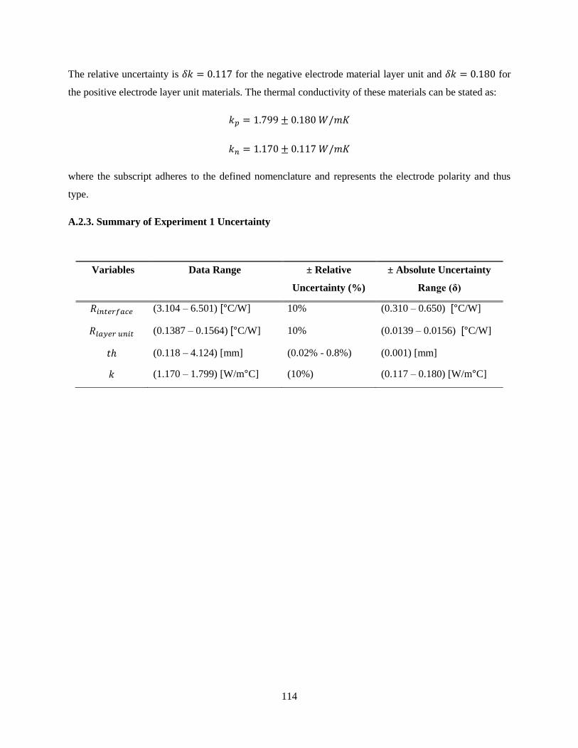
114

The relative uncertainty is for the negative electrode material layer unit and for

the positive electrode layer unit materials. The thermal conductivity of these materials can be stated as:

where the subscript adheres to the defined nomenclature and represents the electrode polarity and thus

type.

A.2.3. Summary of Experiment 1 Uncertainty

Variables Data Range ± Relative

Uncertainty (%)

± Absolute Uncertainty

Range (δ)

(3.104 – 6.501) [°C/W] 10% (0.310 – 0.650) [°C/W]

(0.1387 – 0.1564) [°C/W] 10% (0.0139 – 0.0156) [°C/W]

(0.118 – 4.124) [mm] (0.02% - 0.8%) (0.001) [mm]

(1.170 – 1.799) [W/m°C] (10%) (0.117 – 0.180) [W/m°C]

115


In experiment 2, the total heat generated by the cell is determined along with temperature and heat flux at

various locations of the battery surface. The range of uncertainties determined using the following

analysis is organized into a summary table in Section A.3.3.

A.3.1. Average Surface Temperature

The average battery surface temperature was evaluated using Equation (A.9).

∑(

) (A.9)

Evaluating uncertainty of surface temperature measurements and the of area measurements was required

to determine the overall uncertainty of the average surface temperature measurement. The uncertainties

are as follows:

a) Surface Temperature,

Surface temperature measurements were made with T-type SLE (special limits of error)

thermocouples and recorded with a Keithley 2700 data acquisition system. The uncertainty due to

the thermocouple readout is 1 °C, according to manufacturer’s specifications [56]. The

uncertainty is shown as Equation (A.10).

[ ] (A.10)

b) Area,

An electronic digital caliper with a resolution of 0.005 mm was used to measure the positions of

the thermocouples as installed on the battery surface. As , Equation (A.11) was used to

determine the uncertainty in each area.

(

)

(

)

⁄

(A.11)

For the purpose of evaluating uncertainty in the average surface temperature, let represent the

individual ⁄ components of the surface temperature average, where i and j subscripts describe

the particular thermocouple. Equation (A.12) was then used to determine the error in each product.

116

(

)

(

)

(

)

⁄

(A.12)

A relative uncertainty for the average surface temperature was established via equation (A.13). The

highest surface temperature absolute error occurs when the surface temperature is smallest. The range of

relative uncertainty is large and thus was calculated for each operating temperature. These values are

summarized in Table A1.

(

)

(

)

(

)

⁄

(A.13)

TABLE A1: AVERAGE UNCERTAINTY IN SURFACE TEMPERATURE FOR FIVE OPERATING

TEMPERATURES

Operating

Temperature [°C]

± Relative

Uncertainty (%)

± Absolute

Uncertainty [°C]

5 20.3 1.5

15 2.6 0.5

22 1.1 0.4

25 1.2 0.4

35 0.7 0.3

A.3.2. Heat Generation

The uncertainty in total heat generated is made up of the uncertainties of the components that calculate

the heat. It is calculated using Equation (A.14). The uncertainties that make up Equation (A.14) are

presented in following subsections.

(

)

(

)

(

)

⁄

(A.14)

The uncertainty in the rate of total heat generation is calculated using Equation (A.15).

(

)

(

)

(

)

⁄

(A.15)

117

A.3.2.1. Sensible Heat

The sensible heat energy calculation is based on the mass of the battery, battery specific heat capacity and

average surface temperature. The battery mass and specific heat capacity were reported by the

manufacturer and assumed to have no uncertainty. Thus the uncertainty in sensible heat is as shown in

Equation (A.16).

(A.16)

The uncertainty in the rate of sensible heat accumulation is calculated using Equation (A.17).

(

)

(

)

⁄

(A.17)

a) Surface Temperature Difference Uncertainty

The relative uncertainty in surface temperature difference is largest when the temperature

difference is smallest. Equation (A.18) was used to calculate the uncertainty in average surface

temperature differences.

(

)

(

)

⁄

(A.18)

b) Discharge Time

Discharge time was calculated based on the output from the Labview controlled charge/discharge

bench. The uncertainty is taken to be equal to the resolution of the time measurement, and is

therefore taken to be 1 second. The largest uncertainty occurs during the shortest discharge and is

determined using Equation (A.19). The largest uncertainty will be carried through to simplify

further calculations.

(A.19)

A.3.2.2. Cooling Heat

The cooling heat energy calculation is based on the mass flow rate of the cooling fluid, the coolant

specific heat capacity and temperature difference of the coolant between the inlet and outlet of the cooling

118

plates. The uncertainty in coolant flow rate is assumed to be negligible and the uncertainty in cooling heat

energy is determined using Equation (A.20).

(

)

(

)

(

)

⁄

(A.20)

The uncertainty in the rate of sensible heat accumulation is calculated using Equation (A.21)

(

)

(

)

⁄

(A.21)

a) Flow rate Uncertainty

The volumetric flow rate of the cooling fluid was measured with a Microtherm FS1 30-300

mL/min flow meters. Specifications provided by the manufacturer list instrument uncertainty at

6% of full scale error, which is ± 18 mL/min. This uncertainty is equivalent to Equation (A.22).

The highest relative uncertainty will be carried through to simplify further calculations.

[ ] (A.22)

b) Fluid Temperature Difference

The uncertainty associated with the difference in temperature between the inlet and outlet of the

cooling plates was determined using Equation (A.23). The uncertainty in the temperature

measurement at each inlet or outlet is equivalent to the uncertainty previously given as Equation

(A.10). The highest relative uncertainty will be carried through to simplify further calculations.

(

[ ])

(

[ ])

⁄

(A.23)

a) Discharge Time

This uncertainty is equal to that given in Equation (A.19).

A.3.2.3. Environment Heat

The method of determining the environment heat effect is equivalent to the method used to determine heat

removed by the cooling plate. As such, the uncertainty associated with environmental heat gain is

equivalent to the uncertainty in heat removed by the cooling plates.

119

A.3.2.4. Natural Convection Cooling

The cooling heat energy calculation when natural convection cooling was used is based on correlations

for the heat transfer coefficient based on the Rayleigh and Nusselt number. The uncertainty in convection

cooling heat was determined using (A.24).

(

)

(

)

(

)

(

)

⁄

(A.24)

The uncertainty in the rate of convection cooling heat removal is calculated using Equation (A.26).

(

)

(

)

(

)

⁄

(A.25)

a) Heat Transfer Coefficient Uncertainty

The uncertainty in the heat transfer coefficient was determined using Equation (A.26). The

uncertainty in the thermal conductivity of the air was not included as the effect is considered

negligible.

(

)

(

)

⁄

(A.26)

b) Rayleigh number

The uncertainty in the Rayleigh number was calculated with Equation (A.27). The uncertainty in

the thermo-physical properties of the air were excluded from the calculation as the values were

taken from widely available sources and were dynamically defined based on the film temperature

for each time step of data. As such the contribution to overall uncertainty in Rayleigh number was

assumed to be negligible.

(

)

(

)

(

)

(

)

⁄

(A.27)

120

TABLE A2: AVERAGE UNCERTAINTIES THAT GIVE RISE TO UNCERTAINTY IN RAYLEIGH NUMBER

Variable Absolute Uncertainty (%)

1.78

0.24

0.4

1.1

c) Nusselt Number

The uncertainty in the Nusselt number correlation is equivalent to the uncertainty in the Rayleigh

number as in Equation (A.28). The uncertainty in Prandtl number has been ignored based on the

justification described in the preceding Rayleigh number uncertainty.

( ⁄ )

(A.28)

A.3.2.5. Heat Flux

The heat flux at locations was determined from the product of voltage readings made with the Keithley

hardware and the reported sensitivity of the sensor (HFS). The uncertainty in the HFS voltage readings

based on the Keithley specifications in the range of 100 mV is:

(

[ ]) (A.29)

The maximum uncertainty in HFS readings will occur during the maximum voltage measurement. The

uncertainty in an HFS reading is thus:

(A.30)

121


Variable Range Temperature

[°C]

± Relative

Uncertainty (%)

[°C] 5.6 °C – 47 °C – 2.1% - 17.8%

[°C] 5.6 °C – 44.5 °C – 0.48 % - 28.5%

[J] 1817 J - 29554 J 5 28.7 %

15 3.68 %

22 1.56 %

25 1.70 %

35 1.00 %

[W] 0.52 W – 24.06 W 5 28.7 %

15 3.68 %

22 1.56 %

25 1.70 %

35 1.00 %

[mL/min] 170 mL/min – 218 mL/min – 8.3% - 10.6%

[°C] 0.1 °C – 2.6 °C – 0 % – 21.9%

[J] 5992 J – 11162 J – 24.4 %

[W] 2.9 W – 50.6 W – 24.4 %

[J] 3382.5 J – 66991 J – 24.4 %

[W] 4.12 W – 21.61 W – 24.4 %

[J] 3228 J – 4240 J – 0.56 %

[W] 0.95 W – 4.50 W – 0.58 %

[J] 8090 J – 41345 J 5 44.9 %

15 34.7 %

22 24.4 %

25 34.5 %

35 34.5 %

[W] 2.319 W – 58.56 W 5 44.9 %

15 34.7 %

22 24.4 %

25 34.5 %

35 34.5 %

[W/m2 ] 0 W/m

2 - 4994 W/m

2 – 0% - 0.04%

122


In this experiment, the thermo graphic camera was used to identify and quantify thermal gradients along

several vertical traces of the battery surface. The range of uncertainties determined using the following

analysis is organized into a summary table in Section A.4.4.

A.4.1. IR Temperature

The temperature of the battery surface was measured with an S60 ThermaCAM manufactured by FLIR.

Specifications provided by the manufacturer list uncertainty in temperature measurements to be 2% of the

measured value.

(A.31)

A.4.2. Temperature Response

The uncertainty in temperature responses evaluated in experiment 3 is made up of the uncertainties in

temperatures measured by the camera, and the uncertainty in the time period between images. The

uncertainty in the time measurement between images is taken to be half the resolution of the output

timestamp. This uncertainty is shown as Equation (A.32).

(A.32)

The uncertainty in the temperature response of a single point on the evaluated lines, y1, between two time

indexes t1 and t2 is determined using Equation (A.33):

(

)

(

)

(

)

(

)

⁄

(A.33)

where the uncertainty in temperature difference is 0.0283, determined from the root-sum-square of the

uncertainty of two temperatures.

Since the temperature response for the entire line trace was determined by averaging the response

between each pixel and dividing by the total number of the pixels, the uncertainty in the average

temperature response of an entire evaluated line traced down the battery between two time indexes t1 and

t2 is the same as the uncertainty for the response of a single point, as in Equation (A.34).

123

(

)

(

)

(

)

(

)

(A.34)

Similarly, the uncertainty in the average temperature response of an entire evaluated line traced down the

battery for an entire discharge period is the same as the value determined \using Equation (A.35).

(

)

(

)

(

)

(

)

(A.35)

A.4.3. Thermal Gradient

The uncertainty in thermal gradients evaluated in experiment 3 is made up of the uncertainties in

temperatures measured by the camera, and uncertainties in the Δy measured between each temperature

measurement location. In this case, the pixels in the output images corresponded to temperatures, and thus

Δy was determined from the number of pixels divided by the total length of the evaluated line.

The uncertainty in the thermal gradient between two points y1 and y2 at any point in time is determined

using Equation (A.36). The uncertainty in the distance between pixels is equivalent to (0.5/207).

( ⁄ )

( ⁄ )

(

)

(

)

⁄

(A.36)

The uncertainty in the average thermal gradient of an entire evaluated line traced down the battery

between two time indexes ti and ti+1 was determined using Equation (A.37).

( ⁄ )

( ⁄ )

( ⁄ )

( ⁄ )

(A.37)

The uncertainty in the average thermal gradient of an entire evaluated line traced down the battery for an

entire discharge period was determined using Equation (A.38).

124

( ⁄ )

( ⁄ )

( ⁄ )

( ⁄ )

(A.38)


Variable Range ± Relative

Uncertainty (%)

(20 °C – 70 °C) 2 %

– 2.83%

(

)

(0.00735 °C/s – 0.02897 °C/s) 2.02%

(

)

(0.0126 °C/mm – 0.632°C/mm) 2.01%

125

Appendix B: Experiment 1 Data Summary

Experiment 1 Data Summary

126

Test: Positive Electrode Sample (7 Layers)

TABLE B1: 7 LAYER POSITIVE ELECTRODE SAMPLE TEST RESULTS

1st Test 2

nd Test Average

Load [MPa] Q [W] Tj [°C] R [°C/W] Load [MPa] Q [W] Tj [°C] R [°C/W] R [°C/W]

0.06 7.09 41.03 6.26 0.06 5.97 42.11 6.62 6.44

0.13 7.26 40.69 5.98 0.13 6.18 41.10 6.23 6.11

0.20 7.37 40.13 5.72 0.20 6.35 39.66 5.84 5.78

0.27 7.43 39.56 5.53 0.27 6.91 38.69 5.46 5.50

0.34 7.45 38.96 5.38 0.34 7.44 39.66 5.35 5.36

0.69 8.10 39.08 4.67 0.69 8.13 39.24 4.68 4.67

1.03 8.09 38.24 4.49 1.03 8.15 38.42 4.47 4.48

1.38 8.67 38.99 4.05 1.38 8.49 38.58 4.16 4.10

FIGURE B1: THERMAL RESITSANCE EXPERIMENTAL DATA FOR 7 LAYER POSITIVE ELECTRODE

SAMPLE

0.00

1.00

2.00

3.00

4.00

5.00

6.00

7.00

0.00 0.20 0.40 0.60 0.80 1.00 1.20 1.40 1.60

Th

erm

al

Res

ista

nce

[K/W

]

Contact Pressure [MPa]

1st Test 2nd Test

127



1st Test 2

nd Test Average


0.07 7.58 42.05 6.09 0.06 7.61 42.13 6.04 6.06

0.13 7.69 41.31 5.77 0.14 7.69 41.45 5.78 5.77

0.20 7.73 40.67 5.56 0.20 7.72 40.86 5.60 5.58

0.27 7.72 40.07 5.41 0.27 7.72 40.30 5.46 5.43

0.34 7.70 39.55 5.30 0.34 7.71 39.79 5.34 5.32

0.69 7.81 38.61 4.91 0.69 7.85 38.88 5.00 4.95

1.03 7.77 38.15 4.85 1.03 7.81 38.44 4.95 4.90

1.38 8.00 38.54 4.67 1.38 8.04 38.89 4.79 4.73


SAMPLE

0.00

1.00

2.00

3.00

4.00

5.00

6.00

7.00

0.00 0.20 0.40 0.60 0.80 1.00 1.20 1.40 1.60

Th

erm

al

Res

ista

nce

[K/W

]


1st Test 2nd Test

128



1st Test 2

nd Test Average


0.06 4.44 41.94 7.23 0.07 6.14 40.26 6.57 6.90

0.13 4.54 41.74 7.01 0.14 6.14 38.93 6.38 6.69

0.20 4.64 41.03 6.84 0.21 6.18 38.42 6.22 6.53

0.27 4.69 40.38 6.54 0.27 6.77 40.59 5.94 6.24

0.34 4.70 39.42 6.43 0.34 6.76 40.26 5.89 6.16

0.69 5.21 38.53 6.13 0.68 6.89 39.70 5.67 5.90

1.03 5.83 39.19 5.82 1.03 6.95 39.15 5.54 5.68

1.38 6.25 39.26 5.70 1.37 6.96 38.73 5.46 5.58


SAMPLE

0.00

1.00

2.00

3.00

4.00

5.00

6.00

7.00

8.00

0.00 0.20 0.40 0.60 0.80 1.00 1.20 1.40 1.60

Th

erm

al

Res

ista

nce

[K/W

]


1st Test 2nd Test

129



1st Test 2

nd Test Average


0.06 6.22 42.10 8.24 0.06 5.90 39.57 8.06 8.12

0.13 6.29 41.54 7.92 0.13 5.95 38.79 7.74 7.79

0.20 6.33 40.94 7.66 0.20 5.97 38.14 7.49 7.51

0.27 6.35 40.41 7.48 0.27 6.35 39.18 7.15 7.28

0.34 6.35 39.91 7.32 0.34 6.32 38.84 7.10 7.16

0.69 6.44 39.12 6.94 0.69 6.61 39.01 6.71 6.77

1.03 6.45 38.46 6.75 1.03 6.57 38.55 6.65 6.60

1.38 6.68 38.95 6.51 1.38 6.81 39.26 6.49 6.50


SAMPLE

0.00

1.00

2.00

3.00

4.00

5.00

6.00

7.00

8.00

9.00

0.00 0.20 0.40 0.60 0.80 1.00 1.20 1.40 1.60

Th

erm

al

Res

ista

nce

[K/W

]


1st Test 2nd Test

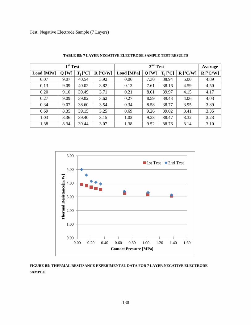
130

Test: Negative Electrode Sample (7 Layers)

TABLE B5: 7 LAYER NEGATIVE ELECTRODE SAMPLE TEST RESULTS

1st Test 2

nd Test Average


0.07 9.07 40.54 3.92 0.06 7.30 38.94 5.00 4.89

0.13 9.09 40.02 3.82 0.13 7.61 38.16 4.59 4.50

0.20 9.10 39.49 3.71 0.21 8.61 39.97 4.15 4.17

0.27 9.09 39.02 3.62 0.27 8.59 39.43 4.06 4.03

0.34 9.07 38.60 3.54 0.34 8.58 38.77 3.95 3.89

0.69 8.35 39.15 3.25 0.69 9.26 39.02 3.41 3.35

1.03 8.36 39.40 3.15 1.03 9.23 38.47 3.32 3.23

1.38 8.34 39.44 3.07 1.38 9.52 38.76 3.14 3.10

FIGURE B5: THERMAL RESITSANCE EXPERIMENTAL DATA FOR 7 LAYER NEGATIVE ELECTRODE

SAMPLE

0.00

1.00

2.00

3.00

4.00

5.00

6.00

0.00 0.20 0.40 0.60 0.80 1.00 1.20 1.40 1.60

Th

erm

al

Res

ista

nce

[K/W

]


1st Test 2nd Test

131



1st Test 2

nd Test Average


0.06 7.10 40.47 6.80 0.07 6.83 42.09 7.10 7.06

0.14 7.31 39.52 6.22 0.13 7.03 41.32 6.57 6.50

0.20 7.40 38.62 5.84 0.20 7.16 40.45 6.11 6.06

0.27 7.80 38.93 5.36 0.27 7.20 39.63 5.80 5.69

0.34 7.77 38.45 5.28 0.34 7.21 38.91 5.59 5.52

0.69 8.36 38.57 4.64 0.68 7.73 38.81 4.83 4.74

1.03 8.34 38.94 4.41 1.03 7.72 38.14 4.68 4.54

1.37 8.62 38.52 4.37 1.38 8.12 38.94 4.41 4.39


SAMPLE

0.00

1.00

2.00

3.00

4.00

5.00

6.00

7.00

8.00

0.00 0.20 0.40 0.60 0.80 1.00 1.20 1.40 1.60

Th

erm

al

Res

ista

nce

[K/W

]


1st Test 2nd Test

132



1st Test 2

nd Test Average


0.06 6.37 41.19 8.04 0.06 6.55 42.07 7.48 7.85

0.14 6.54 40.14 7.43 0.13 6.70 41.67 7.14 7.41

0.20 6.63 39.12 7.02 0.20 6.81 41.14 6.78 7.00

0.27 6.67 38.32 6.74 0.27 6.87 40.64 6.54 6.74

0.34 7.20 39.72 6.33 0.34 6.88 40.13 6.35 6.46

0.69 7.33 38.73 5.95 0.69 7.02 39.10 5.83 5.94

1.03 7.73 38.97 5.52 1.03 7.00 38.14 5.57 5.58

1.38 7.71 38.37 5.44 1.38 7.32 38.72 5.27 5.36


SAMPLE

0.00

1.00

2.00

3.00

4.00

5.00

6.00

7.00

8.00

9.00

0.00 0.20 0.40 0.60 0.80 1.00 1.20 1.40 1.60

Th

erm

al

Res

ista

nce

[K/W

]


1st Test 2nd Test

133



1st Test 2

nd Test Average


0.06 6.12 40.91 8.82 0.06 5.85 42.05 8.54 8.68

0.13 6.43 40.38 8.13 0.13 6.02 41.63 8.05 8.09

0.20 6.63 40.22 7.75 0.20 6.15 41.09 7.62 7.68

0.27 6.76 39.94 7.45 0.27 6.21 40.50 7.32 7.39

0.34 6.85 39.69 7.23 0.34 6.24 39.96 7.11 7.17

0.69 7.24 39.17 6.48 0.69 6.38 38.58 6.47 6.47

1.03 7.34 38.48 6.13 1.03 6.79 39.29 6.04 6.09

1.38 7.71 39.03 5.79 1.37 6.77 38.83 5.97 5.88


SAMPLE

0.00

1.00

2.00

3.00

4.00

5.00

6.00

7.00

8.00

9.00

10.00

0.00 0.20 0.40 0.60 0.80 1.00 1.20 1.40 1.60

Th

erm

al

Res

ista

nce

[K/W

]


1st Test 2nd Test

134

Appendix C: Experiment 2 Results

Experiment 2 Results

135

C.1. Effect of Cooling Temperature on Heat Generation

FIGURE C1: EFFECT OF BATTERY DISCHARGE RATE ON THE HEAT GENERATION PROFILE OF THE TEST

BATTERY AT AN OPERATING TEMPERATURE OF 5 °C



0

10

20

30

40

50

60

70

80

90

100

0 0.1 0.2 0.3 0.4 0.5 0.6 0.7 0.8 0.9 1

Hea

t G

enea

rtio

n R

ate

[W

]

Depth of Discharge

1C - 5°C

2C - 5°C

3C - 5°C

4C - 5°C

-10

0

10

20

30

40

50

60

70

80

90

100

0 0.1 0.2 0.3 0.4 0.5 0.6 0.7 0.8 0.9 1

Hea

t G

enea

rtio

n R

ate

[W

]

Depth of Discharge

1C - 15°C

2C - 15°C

3C - 15°C

4C - 15°C

136





-10

0

10

20

30

40

50

60

70

80

90

0 0.1 0.2 0.3 0.4 0.5 0.6 0.7 0.8 0.9 1

Hea

t G

enea

rtio

n R

ate

[W

]

Depth of Discharge

1C - 25°C

2C - 25°C

3C - 25°C

4C - 25°C

-10

0

10

20

30

40

50

60

0 0.1 0.2 0.3 0.4 0.5 0.6 0.7 0.8 0.9 1

Hea

t G

enea

rtio

n R

ate

[W

]

Depth of Discharge

1C - 35°C

2C - 35°C

3C - 35°C

4C - 35°C

137

C.2. Discharge Data Tables

TABLE C1: 1C DISCHARGE DATA (5 °C COOLING, 240 SECOND INTERVAL)

Charge Voltage [V] 3.6 3.6 3.6 3.6 3.6 3.6 3.6 3.6 3.6 3.6 3.6 3.6 3.6 3.6

Battery Voltage [V] 3.39 3.06 3.05 3.04 3.02 3 3 2.98 2.95 2.9 2.81 2.63 2.35 2.33

Charge Current [A] 0.02 0.01 0.01 0.01 0.02 0.01 0.01 0.02 0.01 0.02 0.01 0.01 0.01 19.99

Discharge Current [A] 20.00 20.07 20.06 20.09 20.06 20.03 20.07 20.10 20.00 20.03 20.06 20.03 20.03 0.22

Time [s] 0 240 480 720 960 1200 1440 1680 1921 2160 2401 2641 2880 3102

1,1 [°C] 6.3 6.8 7.1 7.2 7.3 7.3 7.3 7.4 7.4 7.5 7.8 8.2 8.8 9.5

1,2 [°C] 6.1 6.6 7.0 7.1 7.2 7.2 7.2 7.3 7.3 7.4 7.6 8.1 8.8 9.5

1,3 [°C] 6.3 6.8 7.1 7.3 7.3 7.4 7.4 7.4 7.5 7.6 7.8 8.1 8.7 9.4

2,1 [°C] 6.0 6.4 6.6 6.7 6.8 6.8 6.9 6.9 6.9 7.1 7.3 7.7 8.4 9.1

2,2 [°C] 5.9 6.3 6.5 6.6 6.6 6.7 6.7 6.7 6.7 6.8 7.0 7.4 8.0 8.7

3,1 [°C] 5.9 6.3 6.6 6.8 6.8 6.8 6.8 6.8 6.9 7.1 7.3 7.9 8.8 9.8

3,2 [°C] 5.8 6.2 6.5 6.6 6.7 6.8 6.8 6.8 6.8 7.0 7.3 7.8 8.7 9.8

3,3 [°C] 5.7 6.1 6.3 6.4 6.5 6.5 6.5 6.5 6.5 6.6 6.9 7.4 8.1 9.0

4,1 [°C] 5.6 6.0 6.3 6.4 6.4 6.5 6.5 6.5 6.5 6.7 7.0 7.6 8.6 9.7

5,1 [°C] 5.7 6.2 6.5 6.6 6.7 6.7 6.7 6.7 6.8 7.0 7.4 8.1 9.3 9.5

HFS 1 [W/m2] 267.7 405.5 486.3 519.5 530.8 537.0 545.4 553.3 563.6 588.9 633.2 712.4 826.2 954.7

HFS 2 [W/m2] 299.5 411.1 489.6 526.5 542.7 551.6 560.1 571.8 585.0 616.0 666.3 757.9 889.6 1030.5

HFS 3 [W/m2] 77.8 167.3 217.0 240.1 249.7 251.7 252.2 256.5 265.1 292.2 343.8 442.1 596.2 786.9

Plate 1 Inlet [°C] 5.7 5.7 5.7 5.7 5.6 5.6 5.7 5.7 5.7 5.7 5.7 5.7 5.7 5.7

Plate 1 Outlet [°C] 6.9 7.0 7.0 7.0 7.0 7.0 7.1 7.0 7.0 7.0 7.1 7.1 7.2 7.3

Plate 2 Inlet [°C] 5.6 5.5 5.6 5.6 5.5 5.6 5.6 5.5 5.5 5.5 5.5 5.5 5.5 5.5

Plate 2 Outlet [°C] 6.6 6.6 6.6 6.7 6.6 6.7 6.7 6.7 6.7 6.7 6.7 6.7 6.9 7.0

Average Surface Temperature [°C] 5.8 6.2 6.5 6.6 6.7 6.7 6.7 6.7 6.8 7.0 7.2 7.8 8.7 9.7

138


Charge Voltage [V] 3.6 3.6 3.6 3.6 3.6 3.6 3.6 3.6 3.6 3.6

Battery Voltage [V] 3.12 2.85 2.82 2.75 2.72 2.67 2.61 2.39 2.01 2.57

Charge Current [A] 0.02 0.01 0.01 0.01 0.01 0.01 0.01 0.02 0.02 19.99

Discharge Current [A] 39.96 40.03 40.07 39.98 40.01 40.03 40.02 40.01 40.09 0.07

Time [s] 1 181 361 541 720 900 1081 1261 1441 1447

1,1 [°C] 6.4 7.8 9.1 10.0 10.8 11.4 12.0 12.7 13.9 14.0

1,2 [°C] 6.2 7.9 9.2 10.0 10.6 11.0 11.5 12.3 13.6 13.6

1,3 [°C] 6.4 8.2 9.5 10.2 10.7 11.1 11.4 12.0 13.1 13.2

2,1 [°C] 6.1 7.3 8.3 8.8 9.3 9.7 10.2 10.9 12.3 12.3

2,2 [°C] 5.9 7.2 8.2 8.6 8.9 9.2 9.5 10.1 11.3 11.3

3,1 [°C] 6.0 7.4 8.3 8.8 9.2 9.5 10.0 10.9 12.8 12.9

3,2 [°C] 5.9 7.3 8.3 8.9 9.2 9.5 9.9 10.9 12.7 12.9

3,3 [°C] 5.7 7.0 7.8 8.2 8.5 8.7 9.0 9.8 11.4 11.4

4,1 [°C] 5.6 7.0 7.8 8.2 8.4 8.6 9.0 10.0 12.3 12.4

5,1 [°C] 5.8 7.2 8.2 8.6 8.8 8.9 9.4 10.7 13.5 13.73

HFS 1 [W/m2] 261.3 730.8 1063.1 1259.1 1391.6 1491.5 1584.4 1722.7 1969.6 1981.8

HFS 2 [W/m2] 308.9 656.1 963.4 1202.6 1468.3 1670.0 1829.3 2015.8 2318.1 2331.3

HFS 3 [W/m2] 79.9 357.9 535.9 629.4 693.3 750.3 839.1 1020.9 1396.4 1414.3

Plate 1 Inlet [°C] 5.7 5.7 5.7 5.6 5.7 5.7 5.7 5.6 5.6 5.7

Plate 1 Outlet [°C] 7.1 7.2 7.3 7.4 7.5 7.5 7.5 7.6 7.8 7.8

Plate 2 Inlet [°C] 5.6 5.7 5.7 5.7 5.7 5.7 5.7 5.7 5.7 5.7

Plate 2 Outlet [°C] 6.7 6.9 7.0 7.1 7.2 7.3 7.3 7.4 7.6 7.6

Average Surface Temperature [°C] 5.9 7.3 8.2 8.7 9.0 9.3 9.7 10.7 12.7 12.8

139


Charge Voltage [V] 3.6 3.6 3.6 3.6 3.6 3.6 3.6 3.6 3.6

Battery Voltage [V] 3 2.51 2.62 2.55 2.52 2.48 2.41 2.22 2.81

Charge Current [A] 0.02 0.01 0.01 0.01 0.01 0.01 0.01 0.01 19.29

Discharge Current [A] 59.798 60.043 60.036 60.011 60.05 60 60.032 60.03 0.048

Time [s] 0 121 241 361 481 601 721 841 917

1,1 [°C] 6.3 8.0 11.0 13.0 14.2 15.2 16.0 16.7 17.4

1,2 [°C] 6.1 8.3 11.5 13.3 14.5 15.2 15.9 16.7 17.3

1,3 [°C] 6.3 8.8 12.2 14.0 15.1 15.8 16.4 17.0 17.5

2,1 [°C] 5.9 7.4 9.6 10.9 11.9 12.5 13.1 13.9 14.6

2,2 [°C] 5.8 7.4 9.7 10.9 11.5 12.0 12.5 13.1 13.7

3,1 [°C] 5.8 7.4 9.4 10.7 11.6 12.1 12.7 13.8 14.9

3,2 [°C] 5.7 7.4 9.6 10.8 11.6 12.1 12.7 13.7 14.8

3,3 [°C] 5.6 7.0 8.9 10.0 10.6 11.0 11.4 12.3 13.2

4,1 [°C] 5.5 7.0 8.7 9.7 10.2 10.6 11.1 12.3 13.6

5,1 [°C] 5.6 7.3 9.1 10.0 10.5 10.9 11.5 13.0 14.8

HFS 1 [W/m2] 252.2 1007.9 1919.8 2425.4 2758.3 2967.6 3102.8 3239.4 3348.3

HFS 2 [W/m2] 290.2 747.9 1564.3 2187.1 2622.7 2943.6 3180.5 3417.8 3590.6

HFS 3 [W/m2] 75.3 402.9 837.5 1094.3 1245.9 1356.2 1476.5 1686.0 1913.0

Plate 1 Inlet [°C] 5.6 5.6 5.7 5.7 5.7 5.7 5.7 5.7 5.7

Plate 1 Outlet [°C] 6.9 7.0 7.2 7.4 7.5 7.6 7.7 7.8 7.9

Plate 2 Inlet [°C] 5.6 5.6 5.6 5.6 5.6 5.6 5.6 5.6 5.7

Plate 2 Outlet [°C] 6.6 6.7 7.0 7.3 7.4 7.5 7.6 7.8 7.9

Average Surface Temperature [°C] 5.7 7.4 9.4 10.6 11.3 11.8 12.4 13.4 14.6

140


Charge Voltage [V] 3.6 3.6 3.6 3.6 3.6 3.6 3.6 3.6 3.6 3.6 3.6 3.6 3.6

Battery Voltage [V] 3.54 2.43 2.45 2.46 2.45 2.45 2.53 2.51 2.48 2.41 2.31 2.12 2.66

Charge Current [A] 0.23 0.01 0.02 0.01 0.01 0.01 0.02 0.02 0.02 0.02 0.01 0.02 19.99

Discharge Current [A] 0.105 80.036 80.027 80.018 80.027 80.036 80.027 80.014 80.004 80.03 80.03 80.018 0.002

Time [s] 0 60 121 180 240 301 360 420 481 541 600 661 709

1,1 [°C] 5.8 6.8 9.2 11.5 13.5 15.2 16.5 17.6 18.4 19.1 19.8 20.4 21.0

1,2 [°C] 5.7 6.9 9.9 12.4 14.4 15.9 17.1 18.0 18.5 19.0 19.5 20.1 20.7

1,3 [°C] 5.9 7.1 10.7 13.3 15.4 17.0 18.1 18.7 19.0 19.3 19.6 20.0 20.5

2,1 [°C] 5.5 6.4 8.3 10.0 11.4 12.6 13.5 14.2 14.8 15.4 16.0 16.8 17.5

2,2 [°C] 5.4 6.3 8.5 10.2 11.6 12.6 13.2 13.7 14.0 14.3 14.7 15.2 15.8

3,1 [°C] 5.5 6.5 8.4 10.0 11.3 12.3 13.1 13.8 14.5 15.1 15.9 17.1 18.3

3,2 [°C] 5.3 6.4 8.5 10.2 11.5 12.4 13.2 13.8 14.3 14.9 15.6 16.7 17.9

3,3 [°C] 5.2 6.1 8.0 9.5 10.6 11.4 12.0 12.5 12.9 13.3 13.9 14.8 15.8

4,1 [°C] 5.1 6.2 8.0 9.4 10.3 11.0 11.5 12.0 12.4 13.0 13.8 15.2 16.9

5,1 [°C] 5.3 6.4 8.4 9.9 10.9 11.6 12.1 12.5 13.0 13.6 14.6 16.4 18.6

HFS 1 [W/m2] 239.0 664.8 1646.8 2397.7 3003.9 3487.2 3827.7 3964.7 4021.4 4082.1 4140.8 4231.0 4339.8

HFS 2 [W/m2] 286.8 558.4 1193.4 1886.6 2533.0 3081.1 3531.9 3903.7 4197.6 4441.0 4641.1 4833.3 4994.5

HFS 3 [W/m2] 72.9 309.3 727.1 1085.1 1369.7 1584.6 1746.7 1880.1 1993.2 2114.4 2269.0 2510.0 2784.9

Plate 1 Inlet [°C] 5.1 5.1 5.1 5.1 5.1 5.1 5.1 5.1 5.1 5.1 5.1 5.1 5.1

Plate 1 Outlet [°C] 6.3 6.3 6.4 6.6 6.7 6.9 6.9 7.0 7.1 7.2 7.2 7.3 7.5

Plate 2 Inlet [°C] 5.1 5.1 5.1 5.1 5.1 5.1 5.1 5.1 5.1 5.1 5.1 5.2 5.1

Plate 2 Outlet [°C] 6.0 6.1 6.3 6.6 6.8 7.0 7.1 7.2 7.3 7.4 7.5 7.6 7.7

Average Surface

Temperature [°C] 5.3 6.4 8.5 10.1 11.4 12.3 13.0 13.5 14.0 14.5 15.3 16.5 17.9

141


Charge Voltage [V] 3.6 3.6 3.6 3.6 3.6 3.6 3.6 3.6 3.6 3.6 3.6 3.6 3.6 3.6 3.6

Battery Voltage [V] 3.54 3.07 3.07 3.06 3.05 3.03 3.02 3.01 3 2.99 2.96 2.91 2.76 2.44 2.35

Charge Current [A] 0.19 0.01 0.01 0.01 0.01 0.02 0.01 0.01 0.01 0.01 0.02 0.02 0.01 0.02 20

Discharge Current [A] 0.00 19.95 19.93 19.89 19.99 19.92 19.99 19.91 19.96 19.99 20.03 19.91 19.90 19.95 0.03

Time [s] 0 241 481 720 960 1201 1441 1680 1920 2161 2401 2640 2880 3120 3321

1,1 [°C] 15.5 16.5 17.5 17.9 18.1 18.1 18.1 18.1 18.2 18.2 18.4 18.5 18.8 19.3 19.9

1,2 [°C] 15.5 16.2 16.8 17.2 17.3 17.3 17.3 17.3 17.4 17.4 17.6 17.7 18.0 18.6 19.2

1,3 [°C] 15.6 16.1 16.5 16.8 16.9 16.9 16.9 16.9 17.0 17.0 17.1 17.3 17.5 18.0 18.6

2,1 [°C] 15.5 16.1 16.7 17.0 17.1 17.1 17.1 17.1 17.1 17.2 17.3 17.5 17.8 18.3 19.0

2,2 [°C] 15.5 15.8 16.2 16.4 16.4 16.5 16.5 16.4 16.5 16.5 16.7 16.8 17.1 17.6 18.3

3,1 [°C] 15.5 16.0 16.5 16.7 16.8 16.9 16.8 16.8 16.8 16.9 17.1 17.3 17.7 18.4 19.5

3,2 [°C] 15.4 15.8 16.3 16.5 16.6 16.6 16.6 16.5 16.6 16.6 16.8 17.0 17.4 18.2 19.3

3,3 [°C] 15.4 15.7 16.0 16.1 16.2 16.2 16.2 16.1 16.2 16.3 16.4 16.6 16.9 17.5 18.5

4,1 [°C] 15.3 15.6 15.9 16.0 16.1 16.1 16.1 16.0 16.1 16.2 16.3 16.5 17.0 17.8 19.1

5,1 [°C] 15.4 15.8 16.0 16.2 16.2 16.2 16.2 16.1 16.2 16.3 16.5 16.7 17.3 18.3 19.8

HFS 1 [W/m2] 120.8 252.5 372.9 428.6 455.4 464.4 465.4 466.7 473.7 490.1 513.7 545.4 602.8 718.4 844.1

HFS 2 [W/m2] 129.2 390.1 630.2 732.8 777.4 790.2 788.5 793.8 804.3 828.1 859.0 899.2 968.5 1098.5 1229.8

HFS 3 [W/m2] 40.7 131.4 227.4 272.9 294.8 297.5 286.2 282.5 288.2 309.3 337.0 379.1 451.1 606.6 825.0

Plate 1 Inlet [°C] 15.2 15.1 15.2 15.2 15.1 15.2 15.1 15.1 15.2 15.1 15.2 15.2 15.2 15.2 15.2

Plate 1 Outlet [°C] 15.6 15.8 15.8 15.8 15.8 15.8 15.8 15.8 15.8 15.8 15.9 15.9 15.9 16.0 16.1

Plate 2 Inlet [°C] 15.2 15.2 15.2 15.2 15.2 15.2 15.2 15.1 15.2 15.2 15.2 15.2 15.2 15.2 15.1

Plate 2 Outlet [°C] 15.6 15.7 15.8 15.8 15.8 15.8 15.8 15.8 15.8 15.8 15.9 15.9 15.9 16.0 16.1

Average Surface Temperature

[°C] 15.4 15.8 16.2 16.4 16.5 16.5 16.5 16.4 16.5 16.6 16.7 16.9 17.3 18.1 19.2

142


Charge Voltage [V] 3.6 3.6 3.6 3.6 3.6 3.6 3.6 3.6 3.6 3.6


Charge Current [A] 0.01 0.01 0.02 0.02 0.01 0.02 0.01 0.02 0.01 20.01

Discharge Current [A] 40.02 40.00 39.99 40.01 39.96 39.99 39.97 39.97 40.01 0

Time [s] 10 10 10 10 10 10 10 10 10 9

1,1 [°C] 0 0 0 0 0 0 0 0 0 1

1,2 [°C] 1 180 360 541 720 900 1080 1261 1440 1607

1,3 [°C] 15.3 16.5 18.8 20.1 20.8 21.2 21.5 21.9 22.4 23.3

2,1 [°C] 15.3 16.4 18.2 19.2 19.7 20.0 20.3 20.7 21.2 22.3

2,2 [°C] 15.4 16.4 17.9 18.7 19.2 19.4 19.7 19.9 20.5 21.5

3,1 [°C] 15.3 16.1 17.6 18.5 18.9 19.1 19.4 19.7 20.3 21.5

3,2 [°C] 15.3 16.1 17.1 17.7 18.0 18.2 18.4 18.6 19.2 20.5

3,3 [°C] 15.4 16.2 17.4 18.1 18.5 18.7 18.9 19.3 20.2 22.1

4,1 [°C] 15.3 16.1 17.2 17.9 18.2 18.4 18.6 18.9 19.9 21.8

5,1 [°C] 15.2 15.9 16.7 17.2 17.5 17.6 17.7 18.1 18.8 20.5

HFS 1 [W/m2] 15.2 15.9 16.7 17.1 17.3 17.4 17.5 17.9 18.9 21.2

HFS 2 [W/m2] 15.3 16.1 16.9 17.3 17.4 17.5 17.7 18.1 19.4 22.3

HFS 3 [W/m2] 108.9 395.5 781.9 1000.6 1121.9 1188.4 1239.6 1305.4 1430.3 1678.6

Plate 1 Inlet [°C] 117.7 469.5 1089.2 1465.0 1669.1 1787.8 1890.5 1989.9 2111.4 2355.5

Plate 1 Outlet [°C] 37.3 221.8 470.2 623.9 695.9 725.6 773.8 862.2 1053.0 1484.2

Plate 2 Inlet [°C] 15.0 15.0 15.0 15.0 15.0 15.0 15.0 15.0 15.0 15.0

Plate 2 Outlet [°C] 15.4 15.5 15.7 15.7 15.8 15.8 15.8 15.9 15.9 16.1


143


Charge Voltage [V] 3.6 3.6 3.6 3.6 3.6 3.6 3.6 3.6 3.6 3.6


Charge Current [A] 0.19 0.01 0.02 0.01 0.01 0.01 0.01 0.01 0.01 20

Discharge Current [A] 0.01 60.01 60.00 60.01 60.00 60.02 60.04 59.98 60.03 0.08

Time [s] 0 120 241 361 481 600 720 841 960 1046

1,1 [°C] 15.4 17.6 20.4 22.2 23.3 24.1 24.7 25.3 26.1 27.1

1,2 [°C] 15.4 17.4 19.8 21.4 22.3 22.9 23.5 24.0 25.0 26.1

1,3 [°C] 15.5 17.5 19.6 21.0 21.9 22.4 22.9 23.4 24.2 25.3

2,1 [°C] 15.4 16.9 18.8 20.0 20.8 21.2 21.7 22.3 23.2 24.5

2,2 [°C] 15.3 16.8 18.3 19.3 19.9 20.2 20.6 21.1 22.0 23.3

3,1 [°C] 15.4 17.0 18.5 19.6 20.3 20.8 21.2 21.9 23.4 25.4

3,2 [°C] 15.3 16.9 18.4 19.4 20.0 20.4 20.9 21.6 23.0 25.2

3,3 [°C] 15.3 16.6 17.8 18.6 19.0 19.3 19.7 20.3 21.5 23.3

4,1 [°C] 15.2 16.7 17.8 18.4 18.8 19.0 19.4 20.1 21.8 24.4

5,1 [°C] 15.3 16.9 18.1 18.7 19.0 19.2 19.6 20.4 22.7 26.0

HFS 1 [W/m2] 113.5 699.3 1266.7 1630.7 1860.3 2007.1 2128.1 2255.1 2449.4 2689.4

HFS 2 [W/m2] 136.2 785.8 1601.0 2170.0 2565.8 2838.6 3032.2 3211.4 3447.4 3780.8

HFS 3 [W/m2] 40.2 410.6 760.5 995.6 1139.0 1230.7 1332.7 1493.5 1839.7 2350.5

Plate 1 Inlet [°C] 15.1 15.1 15.1 15.1 15.1 15.1 15.1 15.1 15.1 15.1

Plate 1 Outlet [°C] 15.6 15.7 15.9 16.0 16.1 16.2 16.2 16.3 16.4 16.6

Plate 2 Inlet [°C] 15.1 15.1 15.1 15.1 15.1 15.1 15.1 15.1 15.1 15.1

Plate 2 Outlet [°C] 15.5 15.7 16.0 16.1 16.2 16.3 16.4 16.4 16.5 16.7


144


Charge Voltage [V] 3.6 3.6 3.6 3.6 3.6 3.6 3.6 3.6 3.6 3.6 3.6 3.6 3.6 3.6

Battery Voltage [V] 2.99 2.63 2.69 2.69 2.69 2.69 2.69 2.68 2.66 2.64 2.59 2.49 2.27 2.44

Charge Current [A] 0.01 0.02 0.01 0.01 0.02 0.02 0.01 0.01 0.01 0.01 0.02 0.01 0.01 19.99

Discharge Current [A] 79.791 79.942 79.952 79.975 79.975 79.949 80.014 79.981 79.997 79.981 80 79.984 79.988 76.424

Time [s] 1 60 120 181 241 300 361 420 481 540 601 660 721 780

1,1 [°C] 15.4 15.7 17.4 19.9 21.8 23.4 24.7 25.7 26.5 27.1 27.6 28.1 28.6 29.2

1,2 [°C] 15.3 15.6 17.6 20.0 21.8 23.3 24.4 25.2 25.9 26.4 26.9 27.3 27.8 28.5

1,3 [°C] 15.4 15.8 18.1 20.6 22.3 23.7 24.7 25.5 26.0 26.4 26.8 27.2 27.6 28.2

2,1 [°C] 15.3 15.6 16.9 18.5 19.9 21.0 21.9 22.6 23.1 23.6 24.1 24.5 25.1 26.0

2,2 [°C] 15.3 15.6 17.1 18.7 19.9 20.9 21.6 22.1 22.5 22.8 23.2 23.5 24.0 24.9

3,1 [°C] 15.4 15.7 17.1 18.5 19.7 20.7 21.5 22.1 22.7 23.1 23.6 24.3 25.2 26.7

3,2 [°C] 15.3 15.6 17.1 18.6 19.7 20.7 21.4 21.9 22.4 22.8 23.3 23.8 24.7 26.2

3,3 [°C] 15.2 15.5 16.8 18.0 19.0 19.8 20.3 20.8 21.1 21.4 21.8 22.3 23.0 24.3

4,1 [°C] 15.1 15.5 16.8 18.0 18.8 19.4 19.9 20.2 20.6 20.9 21.2 21.8 22.9 24.8

5,1 [°C] 15.3 15.6 17.1 18.4 19.2 19.8 20.2 20.5 20.8 21.1 21.6 22.3 23.6 26.1

HFS 1 [W/m2] 114.0 238.8 937.7 1623.0 2103.4 2488.6 2767.2 2957.3 3104.1 3218.8 3304.3 3386.0 3474.1 3612.8

HFS 2 [W/m2] 137.5 251.7 797.9 1539.7 2186.8 2733.4 3188.2 3545.9 3826.3 4030.8 4200.9 4343.1 4505.2 4719.2

HFS 3 [W/m2] 39.0 139.7 476.3 827.9 1115.3 1346.8 1528.2 1660.7 1769.3 1864.9 1976.5 2113.4 2327.9 2684.5

Plate 1 Inlet [°C] 15.0 15.0 15.0 15.0 15.0 15.0 15.1 15.1 15.1 15.1 15.1 15.1 15.1 15.1

Plate 1 Outlet [°C] 15.5 15.5 15.6 15.7 15.8 16.0 16.1 16.2 16.3 16.3 16.4 16.5 16.5 16.7

Plate 2 Inlet [°C] 15.0 15.0 15.0 15.0 15.0 15.0 15.1 15.1 15.1 15.1 15.1 15.1 15.1 15.1

Plate 2 Outlet [°C] 15.4 15.5 15.6 15.8 16.0 16.2 16.3 16.4 16.5 16.5 16.6 16.7 16.8 16.9

Average Surface

Temperature [°C] 15.3 15.6 17.1 18.5 19.6 20.5 21.1 21.6 22.0 22.4 22.8 23.4 24.3 25.9

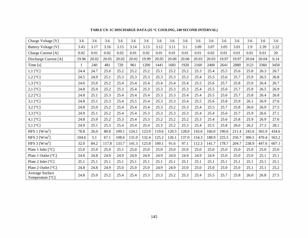
145


Charge Voltage [V] 3.6 3.6 3.6 3.6 3.6 3.6 3.6 3.6 3.6 3.6 3.6 3.6 3.6 3.6 3.6 3.6

Battery Voltage [V] 3.43 3.17 3.16 3.15 3.14 3.13 3.12 3.11 3.1 3.09 3.07 3.05 3.01 2.9 2.39 2.22

Charge Current [A] 0.02 0.01 0.02 0.02 0.01 0.02 0.01 0.01 0.01 0.01 0.02 0.01 0.01 0.01 0.01 20

Discharge Current [A] 19.96 20.02 20.05 20.02 20.02 19.99 20.05 20.00 20.06 20.03 20.03 19.97 19.97 20.04 20.04 0.14

Time [s] 1 240 481 720 961 1200 1441 1681 1920 2160 2400 2641 2880 3121 3360 3450

1,1 [°C] 24.4 24.7 25.0 25.2 25.2 25.2 25.1 25.2 25.2 25.3 25.4 25.5 25.6 25.8 26.3 26.7

1,2 [°C] 24.5 24.9 25.1 25.3 25.3 25.3 25.3 25.3 25.3 25.4 25.5 25.6 25.7 25.9 26.5 26.8

1,3 [°C] 24.6 25.0 25.2 25.4 25.4 25.4 25.4 25.4 25.4 25.5 25.6 25.7 25.8 25.9 26.4 26.7

2,1 [°C] 24.8 25.0 25.2 25.3 25.4 25.3 25.3 25.3 25.3 25.4 25.5 25.6 25.7 25.9 26.5 26.9

2,2 [°C] 24.8 25.1 25.3 25.4 25.4 25.4 25.3 25.3 25.4 25.4 25.5 25.6 25.7 25.8 26.4 26.8

3,1 [°C] 24.8 25.1 25.3 25.4 25.5 25.4 25.3 25.3 25.4 25.5 25.6 25.8 25.9 26.1 26.9 27.6

3,2 [°C] 24.8 25.0 25.2 25.4 25.4 25.4 25.3 25.2 25.3 25.4 25.5 25.7 25.8 26.0 26.9 27.5

3,3 [°C] 24.9 25.1 25.2 25.4 25.4 25.3 25.3 25.3 25.3 25.4 25.4 25.6 25.7 25.9 26.6 27.1

4,1 [°C] 24.8 25.0 25.2 25.3 25.4 25.3 25.2 25.2 25.2 25.3 25.4 25.6 25.8 25.9 26.9 27.6

5,1 [°C] 24.9 25.1 25.3 25.4 25.4 25.4 25.3 25.2 25.3 25.4 25.5 25.8 26.0 26.2 27.3 28.1

HFS 1 [W/m2] 78.8 26.0 80.8 109.1 124.1 123.9 119.6 120.5 128.0 143.6 166.0 190.6 211.4 245.6 365.9 434.6

HFS 2 [W/m2] 104.6 5.1 67.1 108.6 131.0 132.4 125.2 126.1 137.0 154.3 188.9 225.5 256.7 306.5 470.4 563.2

HFS 3 [W/m2] 32.0 84.2 117.8 133.7 141.3 125.8 100.1 91.6 97.1 112.3 141.7 178.7 204.7 238.9 447.6 607.1

Plate 1 Inlet [°C] 25.0 25.0 25.0 25.1 25.0 25.0 25.0 25.0 25.0 25.0 25.0 25.0 25.0 25.0 25.0 25.0

Plate 1 Outlet [°C] 24.8 24.8 24.9 24.9 24.9 24.9 24.9 24.9 24.9 24.9 24.9 25.0 25.0 25.0 25.1 25.1

Plate 2 Inlet [°C] 25.1 25.1 25.1 25.1 25.1 25.1 25.1 25.1 25.1 25.1 25.1 25.1 25.1 25.1 25.1 25.1

Plate 2 Outlet [°C] 24.8 24.8 24.9 25.0 25.0 25.0 24.9 24.9 25.0 25.0 25.0 25.0 25.0 25.1 25.1 25.2

Average Surface

Temperature [°C] 24.8 25.0 25.2 25.4 25.4 25.3 25.3 25.2 25.3 25.4 25.5 25.7 25.8 26.0 26.8 27.5

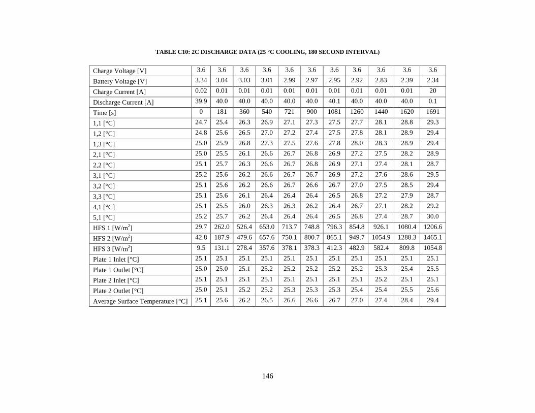
146


Charge Voltage [V] 3.6 3.6 3.6 3.6 3.6 3.6 3.6 3.6 3.6 3.6 3.6

Battery Voltage [V] 3.34 3.04 3.03 3.01 2.99 2.97 2.95 2.92 2.83 2.39 2.34

Charge Current [A] 0.02 0.01 0.01 0.01 0.01 0.01 0.01 0.01 0.01 0.01 20

Discharge Current [A] 39.9 40.0 40.0 40.0 40.0 40.0 40.1 40.0 40.0 40.0 0.1

Time [s] 0 181 360 540 721 900 1081 1260 1440 1620 1691

1,1 [°C] 24.7 25.4 26.3 26.9 27.1 27.3 27.5 27.7 28.1 28.8 29.3

1,2 [°C] 24.8 25.6 26.5 27.0 27.2 27.4 27.5 27.8 28.1 28.9 29.4

1,3 [°C] 25.0 25.9 26.8 27.3 27.5 27.6 27.8 28.0 28.3 28.9 29.4

2,1 [°C] 25.0 25.5 26.1 26.6 26.7 26.8 26.9 27.2 27.5 28.2 28.9

2,2 [°C] 25.1 25.7 26.3 26.6 26.7 26.8 26.9 27.1 27.4 28.1 28.7

3,1 [°C] 25.2 25.6 26.2 26.6 26.7 26.7 26.9 27.2 27.6 28.6 29.5

3,2 [°C] 25.1 25.6 26.2 26.6 26.7 26.6 26.7 27.0 27.5 28.5 29.4

3,3 [°C] 25.1 25.6 26.1 26.4 26.4 26.4 26.5 26.8 27.2 27.9 28.7

4,1 [°C] 25.1 25.5 26.0 26.3 26.3 26.2 26.4 26.7 27.1 28.2 29.2

5,1 [°C] 25.2 25.7 26.2 26.4 26.4 26.4 26.5 26.8 27.4 28.7 30.0

HFS 1 [W/m2] 29.7 262.0 526.4 653.0 713.7 748.8 796.3 854.8 926.1 1080.4 1206.6

HFS 2 [W/m2] 42.8 187.9 479.6 657.6 750.1 800.7 865.1 949.7 1054.9 1288.3 1465.1

HFS 3 [W/m2] 9.5 131.1 278.4 357.6 378.1 378.3 412.3 482.9 582.4 809.8 1054.8

Plate 1 Inlet [°C] 25.1 25.1 25.1 25.1 25.1 25.1 25.1 25.1 25.1 25.1 25.1

Plate 1 Outlet [°C] 25.0 25.0 25.1 25.2 25.2 25.2 25.2 25.2 25.3 25.4 25.5

Plate 2 Inlet [°C] 25.1 25.1 25.1 25.1 25.1 25.1 25.1 25.1 25.2 25.1 25.1

Plate 2 Outlet [°C] 25.0 25.1 25.2 25.2 25.3 25.3 25.3 25.4 25.4 25.5 25.6

Average Surface Temperature [°C] 25.1 25.6 26.2 26.5 26.6 26.6 26.7 27.0 27.4 28.4 29.4

147


Charge Voltage [V] 3.6 3.6 3.6 3.6 3.6 3.6 3.6 3.6 3.6 3.6 3.6


Charge Current [A] 0.02 0.02 0.02 0.01 0.01 0.01 0.02 0.01 0.01 0.01 20


Time [s] 1 121 240 361 481 600 721 841 960 1081 1098

1,1 [°C] 24.6 25.8 27.5 29.1 30.3 31.2 31.9 32.5 32.9 33.7 33.9

1,2 [°C] 24.8 26.2 28.1 29.3 30.2 30.8 31.4 31.9 32.4 33.3 33.5

1,3 [°C] 24.9 26.7 28.9 29.9 30.6 31.0 31.5 32.0 32.5 33.2 33.4

2,1 [°C] 25.0 25.8 26.9 27.9 28.7 29.2 29.7 30.1 30.6 31.6 31.9

2,2 [°C] 25.0 26.1 27.4 28.1 28.5 28.8 29.1 29.5 29.9 30.8 31.0

3,1 [°C] 25.1 25.9 26.9 27.7 28.3 28.7 29.0 29.5 30.2 31.7 32.1

3,2 [°C] 25.0 25.9 27.0 27.7 28.2 28.5 28.8 29.3 30.0 31.4 31.9

3,3 [°C] 25.0 25.8 26.8 27.4 27.7 27.9 28.2 28.6 29.1 30.4 30.8

4,1 [°C] 25.0 25.8 26.5 27.1 27.4 27.5 27.7 28.1 28.8 30.6 31.1

5,1 [°C] 25.1 26.0 26.7 27.2 27.5 27.5 27.8 28.2 29.0 31.3 32.0

HFS 1 [W/m2] 39.5 581.7 1213.3 1511.9 1690.9 1829.1 1957.5 2085.8 2218.1 2416.8 2465.2

HFS 2 [W/m2] 52.7 327.7 918.5 1489.2 1942.1 2253.8 2499.4 2699.5 2845.8 3092.2 3150.3

HFS 3 [W/m2] 11.2 229.2 514.3 717.5 840.4 915.7 1009.9 1133.4 1298.5 1665.5 1782.2

Plate 1 Inlet [°C] 25.0 25.0 25.0 25.0 25.0 25.0 25.0 25.0 25.1 25.0 25.0

Plate 1 Outlet [°C] 24.9 25.0 25.1 25.2 25.3 25.4 25.4 25.4 25.5 25.6 25.7

Plate 2 Inlet [°C] 25.0 25.1 25.1 25.1 25.1 25.1 25.1 25.1 25.1 25.1 25.1

Plate 2 Outlet [°C] 24.9 25.1 25.2 25.4 25.5 25.5 25.6 25.7 25.8 25.9 25.9


148


Charge Voltage [V] 3.6 3.6 3.6 3.6 3.6 3.6 3.6 3.6 3.6 3.6 3.6 3.6 3.6 3.6 3.6

Battery Voltage [V] 2.93 2.76 2.78 2.78 2.75 2.73 2.74 2.74 2.72 2.7 2.68 2.64 2.54 2.28 2.49

Charge Current [A] 0.01 0.01 0.01 0.02 0.02 0.01 0.01 0.01 0.01 0.01 0.01 0.01 0.01 0.01 20.01

Discharge Current

[A] 79.68 80.00 79.97 80.03 80.01 80.02 80.01 80.00 80.02 80.01 79.98 80.02 79.99 80.00 0.41

Time [s] 0 61 121 180 241 300 360 421 480 541 601 660 721 780 824

1,1 [°C] 24.7 25.5 27.1 28.9 30.4 31.6 32.7 33.5 34.1 34.7 35.2 35.6 36.0 36.5 37.0

1,2 [°C] 24.8 25.8 27.6 29.2 30.5 31.6 32.5 33.2 33.7 34.2 34.7 35.1 35.6 36.0 36.6

1,3 [°C] 24.9 26.2 28.1 29.8 30.9 31.9 32.8 33.5 33.9 34.4 34.8 35.2 35.6 36.1 36.6

2,1 [°C] 25.0 25.6 26.7 27.8 28.8 29.6 30.3 30.8 31.2 31.7 32.1 32.5 32.9 33.6 34.4

2,2 [°C] 25.0 25.7 26.9 27.9 28.7 29.3 29.8 30.2 30.5 30.8 31.1 31.5 31.9 32.4 33.2

3,1 [°C] 25.1 25.7 26.7 27.6 28.4 29.0 29.6 30.1 30.4 30.8 31.3 31.8 32.4 33.4 34.7

3,2 [°C] 25.0 25.7 26.7 27.6 28.4 29.0 29.5 29.9 30.2 30.6 31.0 31.4 32.1 33.0 34.4

3,3 [°C] 25.0 25.6 26.5 27.3 27.9 28.4 28.8 29.1 29.4 29.7 30.0 30.4 30.9 31.8 32.9

4,1 [°C] 25.0 25.6 26.4 27.1 27.6 28.0 28.3 28.6 28.8 29.0 29.4 29.8 30.5 31.7 33.4

5,1 [°C] 25.1 25.7 26.6 27.3 27.8 28.2 28.5 28.7 28.9 29.1 29.5 30.0 30.8 32.4 34.6

HFS 1 [W/m2] 37.3 435.1 1050.6 1526.1 1886.2 2197.8 2483.6 2675.2 2814.6 2954.2 3077.9 3185.8 3296.1 3432.5 3591.6

HFS 2 [W/m2] 52.0 257.9 834.6 1468.7 2030.9 2476.0 2842.7 3126.7 3339.9 3532.2 3693.4 3834.2 3967.9 4120.6 4271.0

HFS 3 [W/m2] 10.1 185.5 459.3 720.5 939.8 1110.7 1250.7 1356.9 1443.8 1537.8 1646.1 1772.5 1942.8 2204.0 2579.3

Plate 1 Inlet [°C] 25.0 25.0 25.0 25.0 25.0 25.1 25.1 25.1 25.1 25.1 25.1 25.1 25.1 25.1 25.1

Plate 1 Outlet [°C] 24.9 25.0 25.1 25.2 25.3 25.3 25.4 25.5 25.6 25.6 25.7 25.7 25.8 25.9 26.0

Plate 2 Inlet [°C] 25.1 25.1 25.1 25.1 25.1 25.1 25.1 25.1 25.1 25.2 25.1 25.2 25.1 25.1 25.2

Plate 2 Outlet [°C] 25.0 25.0 25.2 25.3 25.5 25.6 25.7 25.8 25.9 25.9 26.0 26.0 26.1 26.2 26.4

Average Surface

Temperature [°C] 25.0 25.7 26.7 27.6 28.4 28.9 29.4 29.8 30.1 30.4 30.8 31.2 31.8 32.9 34.3

149


Charge Voltage [V] 3.6 3.6 3.6 3.6 3.6 3.6 3.6 3.6 3.6 3.6 3.6 3.6 3.6 3.6 3.6 3.6


Charge Current [A] 0.01 0.01 0.02 0.02 0.01 0.02 0.01 0.01 0.01 0.01 0.01 0.01 0.02 0.01 0.01 20


Time [s] 1 241 480 720 961 1201 1440 1680 1920 2161 2400 2640 2881 3121 3360 3490

1,1 [°C] 33.6 33.8 34.0 34.2 34.2 34.2 34.1 34.1 34.1 34.2 34.3 34.4 34.5 34.5 34.7 34.9

1,2 [°C] 33.9 34.1 34.3 34.4 34.5 34.4 34.4 34.3 34.3 34.4 34.5 34.6 34.7 34.7 34.9 35.2

1,3 [°C] 33.9 34.2 34.4 34.5 34.5 34.5 34.4 34.4 34.4 34.5 34.6 34.7 34.7 34.7 34.9 35.1

2,1 [°C] 34.2 34.3 34.5 34.6 34.6 34.6 34.5 34.5 34.5 34.6 34.7 34.8 34.8 34.9 35.1 35.3

2,2 [°C] 34.4 34.5 34.6 34.7 34.8 34.7 34.7 34.6 34.7 34.7 34.8 34.9 34.9 35.0 35.1 35.4

3,1 [°C] 34.4 34.5 34.7 34.8 34.8 34.7 34.6 34.6 34.6 34.7 34.9 35.0 35.1 35.1 35.3 35.7

3,2 [°C] 34.4 34.5 34.6 34.7 34.8 34.7 34.6 34.6 34.6 34.6 34.8 35.0 35.0 35.0 35.3 35.8

3,3 [°C] 34.5 34.6 34.7 34.8 34.8 34.8 34.7 34.6 34.7 34.7 34.8 35.0 35.0 35.0 35.2 35.6

4,1 [°C] 34.5 34.6 34.7 34.8 34.8 34.7 34.6 34.6 34.6 34.6 34.8 35.0 35.1 35.1 35.4 35.8

5,1 [°C] 34.6 34.7 34.8 34.9 34.9 34.8 34.7 34.6 34.6 34.7 34.9 35.1 35.2 35.2 35.6 36.1

HFS 1 [W/m2] 203.7 109.1 49.8 25.7 17.3 24.5 35.8 35.5 33.8 21.0 3.9 30.3 48.6 52.5 93.8 150.2

HFS 2 [W/m2] 272.0 194.0 124.1 90.4 76.7 83.1 100.6 98.7 96.0 77.5 45.9 6.8 15.3 20.1 79.4 153.9

HFS 3 [W/m2] 62.3 24.6 15.6 34.9 43.5 23.7 1.8 6.4 3.0 14.0 47.8 90.4 110.9 108.4 180.1 297.7

Plate 1 Inlet [°C] 34.6 34.6 34.6 34.6 34.6 34.6 34.6 34.6 34.6 34.6 34.6 34.6 34.6 34.6 34.6 34.6

Plate 1 Outlet [°C] 33.9 33.9 33.9 33.9 33.9 33.9 33.9 33.9 33.9 33.9 33.9 33.9 33.9 33.9 34.0 34.0

Plate 2 Inlet [°C] 34.8 34.7 34.7 34.8 34.8 34.7 34.7 34.8 34.7 34.7 34.7 34.8 34.7 34.7 34.7 34.7

Plate 2 Outlet [°C] 34.1 34.1 34.2 34.2 34.2 34.2 34.2 34.2 34.2 34.1 34.2 34.2 34.2 34.2 34.2 34.3

Average Surface

Temperature [°C] 34.4 34.5 34.6 34.7 34.8 34.7 34.6 34.6 34.6 34.6 34.8 34.9 35.0 35.0 35.3 35.7

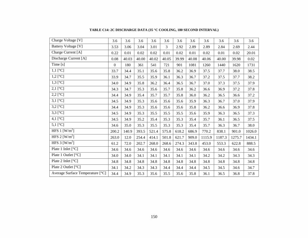
150


Charge Voltage [V] 3.6 3.6 3.6 3.6 3.6 3.6 3.6 3.6 3.6 3.6 3.6

Battery Voltage [V] 3.53 3.06 3.04 3.01 3 2.92 2.89 2.89 2.84 2.69 2.44

Charge Current [A] 0.22 0.01 0.02 0.02 0.01 0.02 0.01 0.02 0.01 0.02 20.01


Time [s] 0 180 361 541 721 901 1081 1260 1440 1620 1731

1,1 [°C] 33.7 34.4 35.1 35.6 35.8 36.2 36.9 37.5 37.7 38.0 38.5

1,2 [°C] 33.9 34.7 35.5 35.9 36.1 36.3 36.7 37.2 37.5 37.7 38.2

1,3 [°C] 34.0 34.9 35.8 36.2 36.4 36.5 36.7 37.0 37.3 37.5 37.9

2,1 [°C] 34.3 34.7 35.3 35.6 35.7 35.8 36.2 36.6 36.9 37.2 37.8

2,2 [°C] 34.4 34.9 35.4 35.7 35.7 35.8 36.0 36.2 36.5 36.6 37.2

3,1 [°C] 34.5 34.9 35.3 35.6 35.6 35.6 35.9 36.3 36.7 37.0 37.9

3,2 [°C] 34.4 34.9 35.3 35.6 35.6 35.6 35.8 36.2 36.6 36.9 37.8

3,3 [°C] 34.5 34.9 35.3 35.5 35.5 35.5 35.6 35.9 36.3 36.5 37.3

4,1 [°C] 34.5 34.9 35.2 35.4 35.3 35.3 35.4 35.7 36.1 36.5 37.5

5,1 [°C] 34.6 35.0 35.3 35.5 35.3 35.3 35.4 35.7 36.3 36.7 38.0

HFS 1 [W/m2] 200.2 140.9 393.5 521.4 575.8 618.2 686.9 770.2 838.1 901.0 1026.0

HFS 2 [W/m2] 263.0 12.0 254.4 414.1 501.8 621.7 909.0 1115.9 1187.3 1275.7 1434.1

HFS 3 [W/m2] 61.2 72.0 202.7 268.0 268.6 274.3 343.8 453.0 553.3 622.8 888.5

Plate 1 Inlet [°C] 34.6 34.6 34.6 34.6 34.6 34.6 34.6 34.6 34.6 34.6 34.6

Plate 1 Outlet [°C] 34.0 34.0 34.1 34.1 34.1 34.1 34.1 34.2 34.2 34.3 34.3

Plate 2 Inlet [°C] 34.8 34.8 34.8 34.8 34.8 34.8 34.8 34.8 34.8 34.8 34.8

Plate 2 Outlet [°C] 34.1 34.2 34.3 34.3 34.4 34.4 34.4 34.5 34.5 34.6 34.7


151


Charge Voltage [V] 3.6 3.6 3.6 3.6 3.6 3.6 3.6 3.6 3.6 3.6 3.6


Charge Current [A] 0.02 0.01 0.01 0.01 0.02 0.02 0.01 0.02 0.01 0.01 20


Time [s] 1 120 241 360 480 601 721 840 961 1080 1145

1,1 [°C] 33.6 34.6 36.9 38.4 39.2 39.6 39.9 40.3 40.7 41.1 41.4

1,2 [°C] 33.9 35.1 37.3 38.5 39.0 39.4 39.7 40.0 40.3 40.7 41.0

1,3 [°C] 33.9 35.6 37.8 38.8 39.3 39.6 39.9 40.1 40.4 40.6 40.9

2,1 [°C] 34.2 34.8 36.2 37.1 37.6 37.9 38.1 38.4 38.8 39.2 39.6

2,2 [°C] 34.4 35.1 36.4 37.1 37.3 37.5 37.7 37.9 38.2 38.5 38.8

3,1 [°C] 34.4 34.9 35.9 36.7 37.1 37.3 37.5 37.8 38.3 38.8 39.4

3,2 [°C] 34.4 34.9 35.9 36.7 37.0 37.2 37.3 37.6 38.1 38.7 39.3

3,3 [°C] 34.5 34.9 35.9 36.4 36.6 36.8 36.9 37.2 37.5 38.0 38.5

4,1 [°C] 34.5 34.9 35.5 36.0 36.2 36.2 36.3 36.6 37.1 37.8 38.6

5,1 [°C] 34.6 35.0 35.6 36.0 36.2 36.2 36.3 36.6 37.2 38.1 39.1

HFS 1 [W/m2] 207.2 456.3 1157.6 1450.0 1595.4 1695.0 1784.3 1861.6 1915.2 1974.8 2062.5

HFS 2 [W/m2] 269.2 130.2 949.9 1461.5 1713.4 1865.4 1986.1 2113.4 2236.1 2357.5 2468.8

HFS 3 [W/m2] 63.2 102.6 418.2 627.3 720.4 757.3 811.7 905.6 1034.9 1158.9 1348.9

Plate 1 Inlet [°C] 34.6 34.6 34.6 34.6 34.6 34.6 34.6 34.5 34.6 34.6 34.6

Plate 1 Outlet [°C] 33.9 33.9 34.1 34.2 34.3 34.3 34.3 34.4 34.4 34.4 34.5

Plate 2 Inlet [°C] 34.7 34.7 34.7 34.8 34.7 34.7 34.7 34.7 34.7 34.7 34.7

Plate 2 Outlet [°C] 34.1 34.2 34.4 34.5 34.6 34.7 34.7 34.7 34.8 34.8 34.9


152


Charge Voltage [V] 3.6 3.6 3.6 3.6 3.6 3.6 3.6 3.6 3.6 3.6 3.6 3.6 3.6 3.6 3.6 3.6


Charge Current [A] 0.02 0.02 0.01 0.01 0.01 0.01 0.01 0.01 0.02 0.02 0.01 0.01 0.01 0.01 0.02 20

Discharge Current

[A] 79.73 80.02 80.03 80.03 80.00 80.03 80.04 80.03 80.03 80.03 80.01 80.03 80.03 80.02 80.02 0.21

Time [s] 1 60 121 180 240 301 360 421 480 541 600 661 720 781 840 857

1,1 [°C] 33.6 33.7 34.9 36.5 38.0 39.3 40.3 41.2 41.8 42.4 42.8 43.2 43.6 43.9 44.1 44.2

1,2 [°C] 33.9 34.0 35.5 37.2 38.6 39.8 40.6 41.2 41.6 42.0 42.4 42.7 43.1 43.3 43.5 43.6

1,3 [°C] 33.9 34.0 36.1 38.1 39.6 40.6 41.3 41.7 42.0 42.3 42.6 42.8 43.1 43.3 43.5 43.5

2,1 [°C] 34.2 34.3 35.0 35.9 36.9 37.7 38.4 38.9 39.3 39.7 40.0 40.3 40.7 41.0 41.3 41.5

2,2 [°C] 34.3 34.4 35.3 36.4 37.3 37.9 38.3 38.6 38.8 39.1 39.3 39.5 39.8 40.0 40.3 40.4

3,1 [°C] 34.4 34.5 35.1 35.8 36.5 37.2 37.7 38.1 38.4 38.7 39.0 39.4 39.8 40.3 40.8 41.1

3,2 [°C] 34.4 34.5 35.1 35.9 36.6 37.3 37.7 38.1 38.3 38.5 38.8 39.1 39.5 40.0 40.6 40.8

3,3 [°C] 34.5 34.5 35.1 35.8 36.5 37.0 37.4 37.6 37.8 38.0 38.2 38.4 38.8 39.2 39.6 39.9

4,1 [°C] 34.5 34.6 35.1 35.6 36.0 36.4 36.7 36.9 37.1 37.3 37.5 37.7 38.1 38.7 39.4 39.8

5,1 [°C] 34.6 34.7 35.2 35.7 36.2 36.5 36.7 36.9 37.1 37.2 37.5 37.8 38.2 38.9 39.9 40.3

HFS 1 [W/m2] 208.5 113.2 682.3 1368.7 1889.9 2215.0 2425.6 2571.3 2670.6 2759.6 2833.4 2902.8 2960.2 3018.1 3077.3 3103.0

HFS 2 [W/m2] 264.3 197.7 235.7 803.3 1351.6 1812.0 2162.4 2450.9 2674.3 2863.3 3018.1 3156.5 3263.9 3340.5 3403.3 3428.9

HFS 3 [W/m2] 61.3 16.9 188.7 426.0 650.1 837.8 972.2 1069.0 1139.3 1212.5 1294.3 1392.2 1502.6 1630.6 1775.7 1846.9

Plate 1 Inlet [°C] 34.5 34.5 34.5 34.6 34.5 34.6 34.5 34.6 34.6 34.6 34.6 34.6 34.6 34.6 34.6 34.6

Plate 1 Outlet [°C] 33.8 33.8 33.8 33.9 34.1 34.1 34.3 34.3 34.4 34.4 34.5 34.5 34.6 34.6 34.7 34.7

Plate 2 Inlet [°C] 34.7 34.6 34.6 34.7 34.7 34.7 34.7 34.7 34.7 34.7 34.7 34.8 34.8 34.8 34.7 34.8

Plate 2 Outlet [°C] 34.0 34.0 34.1 34.3 34.4 34.6 34.7 34.8 34.9 34.9 35.0 35.0 35.1 35.2 35.2 35.3

Average Surface

Temperature [°C] 34.4 34.5 35.2 36.0 36.7 37.3 37.7 38.0 38.2 38.5 38.7 39.0 39.4 39.9 40.5 40.8

153

TABLE C17: 1C DISCHARGE DATA (AIR COOLING ONLY, 240 SECOND INTERVAL)

Charge Voltage [V] 3.8 3.8 3.8 3.8 3.8 3.8 3.8 3.8 3.8 3.8 3.8 3.8 3.8 3.8 3.8 3.8


Charge Current [A] 0.01 0.01 0.02 0.01 0.01 0.01 0.02 0.01 0.01 0.01 0.01 0.02 0.01 0.01 0.01 20


Time [s] 1 241 480 720 961 1201 1441 1680 1920 2161 2401 2640 2881 3120 3361 3409

1,1 [°C] 22.2 22.9 23.7 24.4 24.8 25.1 25.3 25.3 25.4 25.6 25.9 26.4 27.0 28.0 30.0 30.6

1,2 [°C] 22.2 22.8 23.5 24.1 24.5 24.8 24.9 24.9 24.9 25.2 25.5 25.8 26.4 27.4 29.3 30.1

1,3 [°C] 22.3 22.8 23.5 24.0 24.4 24.6 24.8 24.7 24.8 24.9 25.2 25.6 26.1 26.9 28.7 29.3

2,1 [°C] 22.4 22.8 23.6 24.1 24.6 24.7 24.9 24.9 24.9 25.2 25.5 25.9 26.5 27.5 29.6 30.4

2,2 [°C] 22.4 22.9 23.5 24.1 24.5 24.7 24.8 24.8 24.8 25.0 25.4 25.8 26.4 27.3 29.5 30.2

3,1 [°C] 22.4 22.7 23.2 23.5 24.0 24.0 24.2 24.2 24.2 24.4 24.7 25.0 25.5 26.5 28.5 29.3

3,2 [°C] 22.3 22.6 23.2 23.6 24.1 24.1 24.2 24.1 24.2 24.4 24.8 25.0 25.7 26.5 28.7 29.7

3,3 [°C] 22.4 22.8 23.3 23.8 24.1 24.3 24.4 24.4 24.4 24.6 25.0 25.3 26.0 26.9 29.3 29.9

4,1 [°C] 22.2 22.5 22.8 23.1 23.5 23.5 23.6 23.6 23.5 23.9 24.1 24.4 25.0 25.7 28.1 28.8

5,1 [°C] 22.5 22.8 23.2 23.5 23.8 23.9 23.9 23.9 24.0 24.2 24.5 25.0 25.8 26.6 29.2 30.1

HFS 1 [W/m2] 1.6 12.2 24.8 27.5 30.5 42.1 40.4 34.2 41.6 48.7 48.4 54.4 55.8 83.1 92.1 96.5

HFS 2 [W/m2] 0.1 13.0 22.9 42.4 36.6 38.7 36.4 44.1 49.9 46.4 45.2 63.6 60.1 68.8 105.2 105.8

HFS 3 [W/m2] 0.7 11.5 22.6 30.0 37.9 50.4 33.8 39.9 38.8 49.4 55.7 66.4 66.1 96.2 135.7 160.7

Ambient Temperature [°C] 21.4 21.4 21.5 21.7 21.6 21.8 21.5 21.7 21.4 21.7 21.3 21.5 21.7 21.5 21.7 21.8

Average Surface

Temperature [°C] 22.3 22.7 23.2 23.6 24.0 24.1 24.2 24.2 24.2 24.4 24.8 25.1 25.8 26.6 28.9 29.7

154


Charge Voltage [V] 3.8 3.8 3.8 3.8 3.8 3.8 3.8 3.8 3.8 3.8 3.8


Charge Current [A] 0.19 0.01 0.01 0.02 0.02 0.01 0.01 0.01 0.01 0.01 20.01


Time [s] 0 180 360 540 720 901 1081 1261 1440 1620 1692

1,1 [°C] 22.5 24.8 27.9 30.2 31.7 32.6 33.4 34.3 35.5 37.5 39.0

1,2 [°C] 22.6 24.4 26.9 28.9 30.1 31.0 31.7 32.7 33.9 35.9 37.4

1,3 [°C] 22.6 24.4 26.6 28.4 29.6 30.4 31.1 32.0 33.2 35.0 36.7

2,1 [°C] 22.7 24.3 26.6 28.5 29.7 30.6 31.3 32.2 33.4 35.6 37.4

2,2 [°C] 22.8 24.3 26.3 28.1 29.2 30.0 30.8 31.9 33.2 35.5 37.5

3,1 [°C] 22.7 23.7 25.2 26.6 27.4 27.9 28.6 29.5 30.6 32.7 34.7

3,2 [°C] 22.7 23.8 25.3 26.7 27.5 28.3 28.8 29.8 30.8 33.2 35.6

3,3 [°C] 22.8 23.9 25.5 27.0 27.9 28.6 29.4 30.4 31.6 34.1 36.2

4,1 [°C] 22.5 23.4 24.3 25.2 25.9 26.2 26.9 27.8 28.9 31.3 33.7

5,1 [°C] 22.8 23.7 24.8 25.6 26.2 26.7 27.4 28.3 29.6 32.8 35.6

HFS 1 [W/m2] 2.9 45.2 78.1 108.4 133.9 131.7 153.0 182.8 194.9 205.7 237.6

HFS 2 [W/m2] 1.3 42.9 94.4 133.9 138.5 151.5 187.1 194.6 199.8 221.5 252.6

HFS 3 [W/m2] 2.3 42.0 77.9 107.3 128.3 157.5 177.9 188.0 216.8 268.2 334.7

Ambient Temperature [°C] 21.4 21.4 21.4 21.5 21.5 21.5 21.4 21.4 21.5 21.5 21.4


155


Charge Voltage [V] 3.8 3.8 3.8 3.8 3.8 3.8 3.8 3.8 3.8 3.8 3.8


Charge Current [A] 0.02 0.01 0 0.01 0.01 0.01 0.02 0.02 0.01 0.01 20


Time [s] 1 121 240 360 481 601 720 841 960 1081 1125

1,1 [°C] 22.3 25.3 29.4 33.1 36.0 38.0 39.7 41.0 42.8 44.7 45.8

1,2 [°C] 22.4 24.9 28.5 31.6 34.2 35.8 37.5 39.1 40.5 42.7 43.6

1,3 [°C] 22.4 25.1 28.6 31.5 33.8 35.4 37.0 38.4 40.0 41.4 42.7

2,1 [°C] 22.5 24.6 27.7 30.5 32.9 34.6 36.2 37.4 39.3 41.6 43.1

2,2 [°C] 22.6 24.8 27.9 30.5 32.8 34.4 36.0 37.5 39.3 41.8 43.4

3,1 [°C] 22.5 24.1 26.1 28.0 29.5 31.0 32.1 33.1 35.0 37.4 39.4

3,2 [°C] 22.5 24.2 26.3 28.3 30.0 31.2 32.7 34.0 35.7 38.3 40.4

3,3 [°C] 22.6 24.2 26.4 28.5 30.4 31.6 33.0 34.6 36.4 39.3 41.2

4,1 [°C] 22.4 23.7 25.1 26.4 27.4 28.4 29.5 30.5 32.0 35.4 37.3

5,1 [°C] 22.6 24.1 25.5 26.7 27.7 28.5 29.5 30.7 32.3 36.5 38.8

HFS 1 [W/m2] 1.7 77.0 153.5 203.8 241.4 267.4 311.1 314.1 336.0 380.9 367.8

HFS 2 [W/m2] 0.6 60.3 140.6 188.1 240.0 263.9 295.5 355.1 355.2 398.9 428.5

HFS 3 [W/m2] 21.2 21.2 21.2 21.3 21.3 21.2 21.3 21.2 21.3 21.3 21.2

Ambient Temperature [°C] 1.8 48.0 99.3 163.1 203.1 242.5 260.6 313.0 378.9 437.3 501.6


156


Charge Voltage [V] 3.8 3.8 3.8 3.8 3.8 3.8 3.8 3.8 3.8 3.8 3.8 3.8 3.8 3.8 3.8 3.8


Charge Current [A] 0.02 0.01 0.01 0.01 0.02 0.01 0.02 0.02 0.02 0.01 0.02 0.01 0.01 0.01 0.02 19.99


Time [s] 0 60 120 180 241 301 361 420 480 540 600 660 720 781 841 845

1,1 [°C] 22.4 24.5 27.6 30.9 34.1 36.9 39.4 41.6 43.7 45.0 46.9 48.3 49.2 50.6 52.3 52.4

1,2 [°C] 22.5 24.3 27.2 30.1 33.0 35.5 37.7 39.7 41.4 42.9 44.1 46.0 47.3 48.2 50.2 50.4

1,3 [°C] 22.5 24.5 27.5 30.4 33.2 35.5 37.9 39.5 40.9 42.3 43.5 45.1 45.9 47.6 49.0 49.2

2,1 [°C] 22.6 24.2 26.5 28.8 31.3 33.5 35.4 37.3 39.2 40.1 42.0 43.5 44.4 46.3 48.4 48.7

2,2 [°C] 22.6 24.4 26.8 29.4 31.9 34.1 36.3 37.9 39.4 41.0 42.0 43.7 45.3 46.9 49.4 49.6

3,1 [°C] 22.7 23.8 25.4 26.9 28.6 30.1 31.2 32.8 34.2 34.5 36.2 37.6 38.6 40.5 42.3 43.2

3,2 [°C] 22.6 23.9 25.7 27.3 29.2 30.8 32.0 33.5 35.2 35.8 37.4 38.6 39.8 41.5 44.4 45.0

3,3 [°C] 22.7 24.1 25.9 27.6 29.6 31.2 32.9 34.3 35.6 36.8 38.1 39.7 41.3 42.3 46.0 46.1

4,1 [°C] 22.5 23.7 25.1 26.2 27.4 28.3 28.9 30.1 31.2 31.8 32.6 33.7 34.7 36.8 40.5 41.4

5,1 [°C] 22.7 23.9 25.1 26.2 27.0 27.9 28.7 29.4 30.2 30.9 31.5 32.7 33.5 35.9 40.6 41.2

HFS 1 [W/m2] 1.6 64.7 125.8 190.3 257.1 295.6 325.8 356.6 422.9 418.7 462.7 512.5 502.1 574.9 563.3 555.6

HFS 2 [W/m2] 0.6 60.8 122.1 208.5 261.4 291.9 380.6 416.0 430.7 499.3 530.5 527.1 606.8 564.2 588.5 611.3

HFS 3 [W/m2] 5.6 43.5 95.2 144.5 189.0 230.5 263.6 300.8 328.9 390.5 397.2 436.0 477.1 509.4 640.2 646.9

Ambient Temperature [°C] 22.2 22.2 22.2 22.2 22.2 22.2 22.2 22.2 22.2 22.2 22.2 22.2 22.1 22.1 22.2 22.1

Average Surface

Temperature [°C] 22.6 24.0 25.8 27.4 29.1 30.6 31.8 33.2 34.4 35.3 36.4 37.7 38.8 40.7 44.0 44.5

Documents

Experimental Measurements of LiFePO Battery Thermal