Embed Size (px)
Citation preview

EXPERIMENTAL MAIZE FARMING IN
RANGE CREEK CANYON, UTAH
by
Shannon Arnold Boomgarden
A dissertation submitted to the faculty of The University of Utah
in partial fulfillment of the requirements for the degree of
Doctor of Philosophy
Department of Anthropology
The University of Utah
August 2015

Copyright © Shannon Arnold Boomgarden 2015
All Rights Reserved

T h e U n i v e r s i t y o f U t a h G r a d u a t e S c h o o l
STATEMENT OF DISSERTATION APPROVAL
The dissertation of Shannon Arnold Boomgarden
has been approved by the following supervisory committee members:
James F. O’Connell , Chair 22 May 2015
Date Approved
Duncan Metcalfe , Member 19 May 2015
Date Approved
Kevin Jones , Member 27 May 2015
Date Approved
Larry Coats , Member 27 May 2015
Date Approved
Kristen Hawkes , Member 22 May 2015
Date Approved
and by Leslie Ann Knapp , Chair/Dean of
the Department/College/School of Anthropology
and by David B. Kieda, Dean of The Graduate School.

ABSTRACT
Water is arguably the most important resource for successful crop production in
the Southwest. In this dissertation, I examine the economic tradeoffs involved in dry
farming maize vs. maize farming using simple surface irrigation for the Fremont farmers
who occupied Range Creek Canyon, east-central Utah from AD 900 to 1200. To
understand the costs and benefits of irrigation in the past, maize farming experiments are
conducted. The experiments focus on the differences in edible grain yield as the amount
of irrigation water is varied between farm plots. The temperature and precipitation were
tracked along with the growth stages of the experimental crop. The weight of
experimental harvest increased in each plot as the number of irrigations increased. The
benefits of irrigation are clear, higher yields.
The modern environmental constraints on farming in the canyon (precipitation,
temperature, soils, and amount of arable land) were reconstructed to empirically scale
variability in current maize farming productivity along the valley floor based on the
results of the experimental crop. The results of farming productivity under modern
environmental constraints are compared to the past using a tree-ring sequence to
reconstruct water availability during the Fremont occupation of Range Creek Canyon.
The reconstruction of past precipitation using tree ring data show that dry farming would
have been extremely difficult during the period AD 900-1200 in Range Creek Canyon.
Archaeological evidence indicates that the Fremont people were farming during this

period suggesting irrigation was used to supplement precipitation shortfalls.
Large amounts of contiguous arable land, highly suitable for irrigation farming,
are identified along the valley bottom. The distribution of residential sites and associated
surface rock alignment features are analyzed to determine whether the Fremont located
themselves in close proximity to these areas identified as highly suitable for irrigation
farming. Seventy-five percent of the residential sites in Range Creek Canyon are located
near the five loci identified as highly suitable for irrigation farming.
iv

In country such as this, hope’s other name was moisture. Tom Robbins 2001

TABLE OF CONTENTS
ABSTRACT ....................................................................................................................... iii
LIST OF TABLES ............................................................................................................. ix
LIST OF FIGURES .............................................................................................................x
ACKNOWLEDGEMENTS ...............................................................................................xv
Chapters
1. INTRODUCTION .........................................................................................................1
Maize Farming Economics ......................................................................................2 Available Precipitation Thresholds in the Southwest ..............................................5 Dry vs. Irrigation Farming .......................................................................................7 Research Question ...................................................................................................8
Expectations .....................................................................................................9 Objective ........................................................................................................10
Evaluating the Scale of Farming Productivity .......................................................11 The Fremont ...........................................................................................................12 Range Creek Canyon .............................................................................................13
Setting and Background .................................................................................14 Field Station and Field School .......................................................................15 Range Creek Canyon Archaeology ................................................................16 Chronology .....................................................................................................18 Irrigation .........................................................................................................18
2. EXPERIMENTAL MAIZE FARM .............................................................................22
First Year Pilot Study.............................................................................................23 2014 Second Year Experiment ..............................................................................24
Choice of Maize Variety ................................................................................24 Choice of Field Location ................................................................................26 Irrigation Schedule .........................................................................................27
Tracking Soil Moisture ..........................................................................................27 Soil Moisture Sensors .....................................................................................28
Soil Moisture Sensors--Results ..............................................................................30

Control Plot ....................................................................................................30 Experimental Plot 1 ........................................................................................32 Experimental Plot 2 ........................................................................................33 Experimental Plot 3 ........................................................................................36 Experimental Plot 4 ........................................................................................36
Soil Moisture Conclusion ......................................................................................37 Harvesting and Ear Processing--Methods ..............................................................37
Ear and Kernel Analysis .................................................................................38 Harvesting and Ear Processing--Results ................................................................38
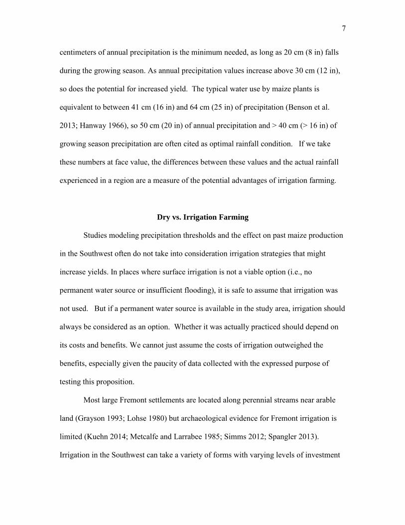
Ear Characteristics ..........................................................................................41 Yield and Water .....................................................................................................45
Sample Adjustments .......................................................................................46 Water and Yield Conclusions ................................................................................50
3. ENVIRONMENTAL CONSTRAINTS ON FARMING ............................................79
Precipitation ...........................................................................................................80
Weather Stations .............................................................................................81 Rain Gauges ...................................................................................................82 PRISM Climate Data ......................................................................................82
Precipitation--Results .............................................................................................84 Thresholds for Dry Farming ...........................................................................85 Recent Precipitation Variability in Range Creek Canyon ..............................86 Regional Precipitation Variability in Range Creek Canyon ..........................89
Seasonality of Temperature in Range Creek Canyon ............................................90 Temperature ....................................................................................................91 Growing Season--Results.......................................................................................94 Frost Free days (FFD) ....................................................................................95 Experimental Crop CGDD ............................................................................ 95 Canyon-wide Estimates of CGDD .................................................................96 Regional Temperature Variability .........................................................................98 Comparing Range Creek CGDD with Other Experiments ..................................100 Muenchrath 1995 ..........................................................................................101 Bellorado 2007 ............................................................................................ 103 Adams et al. 2006 MAIS ..............................................................................104 Comparison to Range Creek CGDD ............................................................105 Precipitation and Temperature Conclusion ..........................................................106 Identifying Arable Land .......................................................................................108 Valley Floor and Slope .................................................................................112 Calculating Amount of Contiguous Arable Land ........................................ 112 Amount of Arable Land--Results.........................................................................114 Soil Texture ..........................................................................................................115 Soil Texture in Farm Plots ............................................................................116 Soil Texture on Canyon Bottom .................................................................. 116 Soil Texture--Results ...........................................................................................117 Field Capacity ...............................................................................................118
vii

Soil Properties from Canyon Floor ............................................................. 119
4. ARCHAEOLOGICAL IMPLICATIONS .................................................................147
Settlement Pattern Studies ...................................................................................148 Behavioral Ecology Approaches to Settlement Pattern Study .....................150
Settlement Patterns in Range Creek Canyon .......................................................154 Modeling Suitability .....................................................................................155
Modern Climate Suitability for Farming .............................................................157 Past Climate Suitability for Farming ...................................................................159
Dry Periods ...................................................................................................161 Wet Periods ..................................................................................................163 Implications for Dry Farming .......................................................................163
Archaeological Expectations for Settlement ........................................................167 Open Residential Sites ..................................................................................168 Distribution of Residential Sites ...................................................................170
Site Density and Arable Land ..............................................................................171 Settlement Patterning Conclusion ........................................................................176
5. FUTURE RESEARCH ..............................................................................................186
Irrigation Cost ......................................................................................................187 Hydrology ............................................................................................................190 Fluvial History .....................................................................................................192 Maize Farming Experiments ................................................................................193
Soil Moisture Sensors ...................................................................................194 Rooting Depth ..............................................................................................195 Other Avenues ..............................................................................................195
Discussion ............................................................................................................196 REFERENCES ................................................................................................................199
viii

LIST OF TABLES
2-1 Comparison of Maize Farming Experiments 2013 and 2014…………………….52
2-2 Precipitation at the Experimental Plots during the Growing Season…………… 58
2-3 Summary of Yields from Experimental Plots in 2013 and 2014……………….. 67
2-4 Results of Ear Descriptive Analysis……………………………………………. 68
2-5 Descriptive Summary of Plot 2 and Plot 3 Yield……………………………… 75
2-6 Descriptive Summary of Yield Samples ………………………..……………… 76
3-1 Total Precipitation from Rain Gauges…………………………………………. 124
3-2 Frost Free Days Compiled by Year and Weather Station……………………… 130
3-3 Cumulative Growing Degree Day Requirements for Maize Hybrid…………....131
3.4 Results of Sedimentation Texture Test in Experimental Plots………………….144
3-5 Results of Canyon-wide Surface Soil Analysis…………………………………146
4-1 Summary of Arable Land Loci and Associated Residential Rock Alignments…184

LIST OF FIGURES
1-1 Illustration of a simple surface irrigation system…………………………………19 1-2 Chart showing a hypothetical sigmoid curve demonstrating the expected increase in yield as a function of available water, either from precipitation or
irrigation. The yield with available precipitation at point A might improve with additional irrigation water if the benefits outweigh the costs. If there is plenty of precipitation to produce the yield at point B, irrigation may not be
profitable………………………………………………………………………... 20 1-3 Relief map showing an overview of the project area…………………………... 21 2-1 Contour map of the Range Creek Field Station headquarters showing the location of the 2014 experimental maize plots………………………………… 53 2-2. Overview of the experimental maize crop facing north on planting day, May 20, 2014. Plots are located in the former orchard of the Range Creek Field Station headquarters……………………………………………………… 54 2-3 Photographs showing the placement of the soil moisture sensors in the experimental plots (left) and an overview of the experimental plots taken facing south, showing sensors aligned down the center (right).……………… 55 2-4 Photographs showing the placement of the soil moisture sensors in the control plot (left) and the application of water to the control plot (right)……... 56 2-5 Chart showing soil moisture data from the sensor control plot. Data are from four sensors, placed at 6 in (6c, blue line), 12 in (12c, red line), 24 in (24c, green line), and 36 in (36c, black line) below the ground surface. Black
arrows indicate the dates that water was added to the plot and the amount in gallons. Blue vertical sections indicate timing and amount of precipitation
received………………………………………………………………………… 57 2-6 Overview photograph showing Plot 1. Plot 1 was irrigated only once, on the day it was planted. The Plot 1 plants dried up and died shortly after June 16, 2014…………………………………………………………………… 59 2-7 Chart showing soil moisture sensor data from Plot 2. Data are from two sensors

placed at 12 in (12e, black line) and 30 in (30e, red line) below ground surface. Vertical arrows indicate irrigation events. Plot 2 was irrigated 8 times during
the growing season (irrigation even on planting day, May 20, 2014 not shown). Blue sections indicate timing and amount of precipitation received. The red area is the timing of critical reproductive stage. The sun symbol indicates the first recorded tassels……………………...…………………………………… 60 2-8 Photographs taken on July 23, 2014, showing maize plants from experimental farm plots. Example of plants in Plot 2, showing stunted growth and severe water stress between irrigation events (left). Photograph of plants from Plot 4 on the same day showing healthy vigorous foliage (right)……………………... 61 2-9 Photographs showing maize plants from Plot 4 (left). These three plants were
excavated from a single basin to examine rooting depth at the end of the growing season. Note the shallow affective root zone, only 25 cm (10 in) below surface including tap roots (right)……………………………………… 62 2-10 Chart showing soil moisture sensor data from Plot 3. Vertical arrows indicate
irrigation events. Plot 3 was irrigated 10 times during the growing season (irrigation event on planting day May 20, 2014 not shown). Blue sections indicate timing and amount of precipitation received. The red area is the timing of critical reproductive stage. The sun symbol indicates the first tasseling recorded……………………...………………………...…………… 63 2-11 Chart showing soil moisture sensor data from Plot 4. Vertical arrows indicate
irrigation events. Plot 4 was irrigated 14 times during the growing season (first irrigation event on planting day May 20, 2014 not shown). Blue sections indicate timing and amount of precipitation received. The red area is the timing of critical reproductive stage. The sun symbol indicates the first
recorded tasseling……...……...………………………...………………………...…… 64
2-12 Overview of experimental farm plots ………………………………………... 65 2-13 Photographs showing overview of a basin and a close up of cobs prior to
harvest..……...……...……...……...……...……...……...……...……...……... 66 2-14 Selection of ears from irrigated experimental plots. (A) Plot 2, (B) Plot 3, (C) Plot 4……………………………………………………………………… 69 2-15 Examples of undeveloped kernels on tips of ears. Mean percentage of kernel
coverage is reported in Table 2-3……………………………………………... 70 2-16 Example of patchy kernel development along the length of the ear. Patchy kernel development is a morphological characteristic likely associated with
environmental stress that occurred more often in Plots 2 and 3………………….71
xi

2-17 Two examples of ears with irregular rows, a morphological characteristic likely associated with environmental stress, was more common in Plots 2 and 3………………...………………………...………………………...……… 72 2-18 Photographs of ears showing pink discoloration ……………………………… 73 2-19 Map showing the location of horse damaged basins in Plot 4 and the location of basins selected for exclusion from Plots 2 and 3…………………………... 74 2-20 Graph showing increase in total grain yield as number of irrigations increase. All plots received 7.37 cm (2.9 in) of rain during the growing season. The data
points between plots were estimated using the surrounding data points……... 77 2-21 Results of maize farming experiment showing total amount of grain yield (g) and amount of irrigation water applied (number of days) for two growing seasons (Adams et al. 1999: Table 1 and Table 8). Data points are labeled using water treatment numbers from Adams et al. 1999. The slope between
irrigation events 5-7 is estimated using the total yield from T2 and T1……… 78 3-1 Relief map of lower Range Creek Canyon showing the location of two automated weather stations and the 11 manual rain gauges. Note the location of the experimental corn field near rain gauge 10…………………… 121 3-2 Mean and range of monthly precipitation values in centimeters from Weather
Station 1 for 2008-2013……………………………………………………... 122 3-3 Total precipitation values in centimeters for growing season months for 2008-2010 and 2012-2013 from Weather Station 1, centrally located in the canyon at an elevation of 1,690 m (5,550 ft). The data set for 2008 includes only July through October. The data set for 2011 was excluded because readings from three months are not available………………………... 123 3-4 Chart showing trend in precipitation totals from the rain gauges located along the canyon bottom. There is a general decrease in amount of precipitation from north to south as elevation decreases. Rain gauge number nine (RG-9) was excluded because it was not placed until 2014…………… 125 3-5 Contour map of the hydrologic basin draining into Range Creek Canyon showing the average precipitation received annually over the last 30 years... 126 3-6 Contour map of the hydrologic basin draining into Range Creek Canyon, showing the average precipitation received from June through September over the last 30 years………………………………………………………… 127 3-7 Contour map of the hydrologic basin draining into Range Creek Canyon, showing average winter precipitation received from November through
xii

March over the last 30 years………...………………………...……………... 128 3-8 Precipitation over the last 30 years modeled from PRISM data. (A) Chart showing the modeled probability distributions for average precipitation received during the growing season over the last 30 years in Range Creek Canyon at five elevations. The vertical black line at 6 in (15 cm) indicates the traditionally cited lower limit of summer precipitation necessary for dry farming maize. (B) Chart summarizes the probability of achieving 15 cm (6 in) of precipitation…………………………...………………………...…… 129 3-9 Chart showing the CGDD for 2009-2014 from Weather Station 1 with a planting date of May 8th (the day after the latest spring freeze for all years)… 132 3-10 Showing the difference in CGDD between Weather Station 1 (mean for years 2009-2014 last spring freeze May 8th) and Weather Station 2 (2014 full year with last spring freeze May 16) with a difference in elevation of 370 m (1,210 ft)……………………………………………………………... 133 3-11 Chart showing the estimated CGDD for increasing elevation and decreasing
temperatures between Weather Station 1(mean for 2009-2014) and Weather Station 2 (2014 only). Note the first fall freeze at Weather Station 2 (2,060 m [6,760 ft] elevation) on October 01, 2014………………………………... 134 3-12 Chart showing the estimated CGDD for increasing elevation and decreasing
temperatures between Weather Station 1 (mean for 2009-2014) and Weather Station 2 (2013 fall). Note the first fall freeze at Weather Station 2 (2,060 m [6,760 ft] elevation) on September 27, 2013………………………………… 135 3-13. Map showing the 2,000 m (6,560 ft) elevation contour in Range Creek Canyon. Based on the CGDD required for the experimental maize to reach full maturity, planting above 2,000 m (6,560 ft) would be risky in cool
years………...………………………...………………………...…………… 136 3-14 Chart showing the modeled probability distributions for average FFD over the last 30 years in Range Creek Canyon at five elevations. (A) The vertical black line indicates the 120 FFD. (B) Chart showing the modeled probability
distributions for average CGDD over the last 30 years in Range Creek Canyon at five elevations. The vertical black line indicates 2250 CGDD......... 137 3-15 Chart showing the probability of achieving ≥ 120 frost free days (FFD) and ≥ 2250 CGDD in Range Creek Canyon at five elevations over the last 30 years
(PRISM dataset 1981-2010)…………………………………………………... 138 3-16 Chart showing the proportional probability of achieving ≥ 1800 CGDD in Range Creek Canyon at five elevations (PRISM dataset 1981-2010)…………. 139
xiii

3-17 Chart showing the probability of receiving ≥ 6 in (15 cm) of precipitation and ≥ 2250 CGDD at five elevations in Range Creek Canyon………………... 140 3-18 Map scaling the contiguous arable land available on the valley floor in Range Creek Canyon. Areas in red have the largest amount of contiguous arable land. Three sections of the topography and associated hotspots for farming are identified………………………………………………………... 141 3-19 Map showing the valley floor in Range Creek Canyon split into three sections and the corresponding loci for contiguous arable land in each
section………...………………………...………………………...…………... 142 3-20 Photograph showing soil profile sample for soil texture analysis, located outside Plot 2………………………………………………………………… 143 3-21 Map of lower Range Creek Canyon showing the location of 21 surface soil samples analyzed for texture and chemistry. Large circles indicate soil texture
determinations for the point sampled and an estimated soil texture for surrounding areas…………………………………………………………… 145 4-1 Map of Range Creek Canyon showing the probability (gray) of receiving the lower limits of precipitation necessary during the growing season for dry
farming (≥ 6 in/15 cm) and the probability of achieving a CGDD ≥ 2250 as a function of elevation……………...…………………………………………… 178
4-2 Graph showing decadal precipitation reconstruction from the Harmon Canyon dendrochronology sequence, Nine Mile Canyon (Knight et al. 2010: adapted from Figure 6:5). Departures above and below the mean (37.6 cm) show extremely wet and dry periods defined as Gaussian-filtered series with standardized values greater than 1.25 in absolute value (Knight et al. 2010)……………...………………………...…………………………... 179 4-3 Chart showing the normal distribution of summer rainfall received in Range Creek Canyon at 1,520 m (5,000 ft) over the last 30 years with a mean of 3.53 in (9 cm) and a standard deviation of 1.19 in (3 cm). That same
normal distribution with a mean of 6 in (15 cm) would require a 170% increase in precipitation to receive the lower threshold for dry farming 50% of the time…………...………………………...……………………………… 180 4-4 Examples of rock alignments at residential sites: (above) coursed wall alignment and (below) a single-course alignment…………………………… 181 4-5 Map of lower Range Creek Canyon showing the density of surface rock alignments. Darker areas have the highest density of rock alignments within a 400 meter radius and areas in white have the lowest number………... 182
xiv

4-6 Map showing variability in amount of contiguous arable land and the density of residential rock alignments in Range Creek Canyon. Patterning associated with three sections of the canyon are identified……………………………... 183 4-7 Map showing the total farmable area in hectares for arable land loci within each section in Range Creek Canyon and the density of rock alignments associated with each loci……………………………………………………… 185 5-1 Example of the areas of the returns curve from the 2014 experimental maize plots that need to be explored further with additional plots and changes in the irrigation schedule. A plot will be added that is watered once every 3-4 weeks, and a plot will be added that is watered every day to test whether yield begins to diminish……………………………………… 198
xv

ACKNOWLEDGEMENTS
I could not have completed this work without my friend and mentor Duncan
Metcalfe. Over the years he has provided ideas, inspiration, critiques, and support that
have been invaluable. I would also like to thank my committee and countless colleagues
for their assistance with data collection, edits, discussions, and endless support including:
Corinne Springer, Isaac Hart, Dave Potter, Andrew Yentsch, Joan Coltrain, Rachelle
Green Handley, Jamie Clark Stott, Kevin Jones, Larry Coats, Andrea Brunnelle, Mitch
Power, Michelle Knoll, Glenna Nielsen, Ellyse Simons, Nicole Herzog, Ashley Grimmes
Parker, and Michael Lewis.
I would like to thank my family, Joel and Folsom Boomgarden, for their love,
support, and patience. I would like to thank my mother, Jamie Weston, for being my
inspiration in all undertakings and teaching me the value of hard work and dedication.
This work could not have been completed without the tireless efforts of the staff
and students of the Range Creek Field School and the support of the Natural History
Museum of Utah and the Department of Anthropology, University of Utah.

CHAPTER 1
INTRODUCTION
For the last 13 years, staff and students of the Range Creek Field Station have
been documenting the archaeological record in Range Creek Canyon, east-central Utah.
We have recorded an intense Fremont occupation of the canyon from AD 900 to 1200. In
addition to identifying archaeological remains, we have focused on learning about the
modern environment and reconstructing the past environment to understand the economic
decisions made by the Fremont living there 1,000 years ago. The archaeological evidence
tells us that they were maize farmers but we suspected, given the wide range of
variability in elevation, precipitation, temperatures, soils, distribution of arable land, and
access to irrigation water along the valley floor, that farming maize was and is still very
difficult in this area. We suspected that the success of maize farming along the valley
floor in Range Creek Canyon likely varied both spatially and temporally. This research
tests these assumptions empirically. The following are the results of maize farming
experiments, reconstruction of modern and past environmental constraints on farming,
and the archaeological patterning in site locations related to the costs and benefits of
farming in Range Creek Canyon.

2
Maize Farming Economics
Water is arguably the most important resource for successful crop production in
the arid Southwest. There is a long tradition in Southwestern archaeology that assumes if
dry farming was possible, then it is what likely was practiced. This view has some
validity but can be expanded to consider irrigation, the artificial management of water, as
a strategy which is likely to have both costs and benefits. When the benefits outweigh
the costs, we should expect prehistoric peoples to consider irrigation a viable and rational
strategy for dealing with the vagaries of farming in an arid or semi-arid environment.
When the costs outweigh the benefits, then irrigation is not a rational strategy. Studies
from behavioral ecology, both in humans and nonhumans, have demonstrated that the
costs and benefits of a particular strategy are strongly conditioned by features of the
natural and social environment in which they occur, and that these features may vary
tremendously through time and across space. In some places, irrigation might be
relatively inexpensive, such as for fields near a permanent creek that is not deeply
entrenched and that have soils easily dug for ditches. The benefits are also likely to vary:
areas that regularly received sufficient quantities of precipitation during all the critical
stages of plant growth and reproduction are not prime candidates no matter how cheap
irrigation is. The important point is that it is a consideration of both the costs and
benefits that allow us to predict where and when we might expect prehistoric farmers to
practice irrigation, and where and when they should not have. In most cases, costs and
benefits will not vary in a coordinated fashion, so the benefits and costs need to be
assessed independently.
3
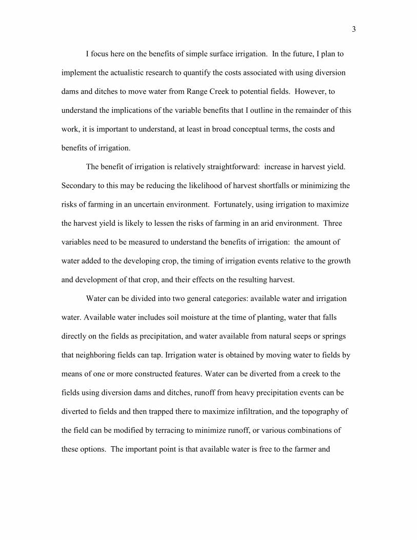
I focus here on the benefits of simple surface irrigation. In the future, I plan to
implement the actualistic research to quantify the costs associated with using diversion
dams and ditches to move water from Range Creek to potential fields. However, to
understand the implications of the variable benefits that I outline in the remainder of this
work, it is important to understand, at least in broad conceptual terms, the costs and
benefits of irrigation.
The benefit of irrigation is relatively straightforward: increase in harvest yield.
Secondary to this may be reducing the likelihood of harvest shortfalls or minimizing the
risks of farming in an uncertain environment. Fortunately, using irrigation to maximize
the harvest yield is likely to lessen the risks of farming in an arid environment. Three
variables need to be measured to understand the benefits of irrigation: the amount of
water added to the developing crop, the timing of irrigation events relative to the growth
and development of that crop, and their effects on the resulting harvest.
Water can be divided into two general categories: available water and irrigation
water. Available water includes soil moisture at the time of planting, water that falls
directly on the fields as precipitation, and water available from natural seeps or springs
that neighboring fields can tap. Irrigation water is obtained by moving water to fields by
means of one or more constructed features. Water can be diverted from a creek to the
fields using diversion dams and ditches, runoff from heavy precipitation events can be
diverted to fields and then trapped there to maximize infiltration, and the topography of
the field can be modified by terracing to minimize runoff, or various combinations of
these options. The important point is that available water is free to the farmer and

4
irrigation water is not. Irrigating requires capital investments as well as maintenance and
operational costs.
The focus of my research is on surface irrigation, specifically moving water from
a surface source, in this case Range Creek, to potential agricultural fields along the
canyon bottom. This type of irrigation typically involves constructing diversion dams
and ditches to divert the water from the creek to the fields. These irrigation systems
range from simple to complex. A simple system is based on a single diversion dam and
one field ditch where the field ditch moves water along the upslope side of the field
(becoming the header ditch, Figure 1-1). More complicated systems include multiple
diversion dams, field ditches, head gates, furrows and tail water ditches. My focus here
is on the simplest surface irrigation system.
The costs of constructing these features will vary as a function of both the
characteristics of the water source and the field, and the distance between the two. It is
clearly less costly to divert water from a creek flowing in a shallow channel than it is to
divert from a deeply incised creek; it is less costly to construct a 100 m field ditch than it
is one twice as long; it is more efficient to spread water across a level and rock-free field
than it is a field filled with large boulders and with an uneven surface. All of these can be
thought of as the capital costs of this type of irrigation, costs that can be amortized over
their useful life. The point is there is no such thing as “the cost” of irrigation because the
cost will be a function of local conditions. Irrigation also has maintenance costs, such as
rebuilding diversion dams damaged during spring or flash floods, cleaning accumulated
silts from ditches, as well as operational costs such as actively distributing irrigation
water throughout the field when irrigating. Both maintenance and operational costs are

5
likely to be less, I suspect in most cases significantly less, than the capital costs, but they
are ongoing costs that accrue over time.
Available Precipitation Thresholds in the Southwest
Farming success is not an either/or proposition, but rather a variable that ranges
from failure to producing the best possible crop. While quantifying the effect of
irrigation on harvest yield, a simple but comprehensive measure of relative success, a
number of other variables are important as well. Clearly soils are important. They must
have sufficient nutrients for crop growth and development and their texture is important
for root development and determines their capacity to hold moisture. Climate variables
are important, especially temperature and precipitation. Crops need water and
appropriate temperatures to grow well. Precipitation can be augmented by irrigation, but
temperatures during the growing season are a function of latitude, elevation, regional and
local topography, and weather patterns. Temperatures and soils are effectively a function
of location, but water may not be. There are also strong interactions between these
variables when it comes to harvest yield, but parsing their effects is the first step to
understanding the opportunities and constraints of prehistoric farming in a particular
place.
Archaeologists studying prehistoric farming in the arid Southwest have typically
employed thresholds to determine whether there was sufficient precipitation to dry farm
successfully (Benson 2010a and 2010b; Benson et al. 2013). Implicit in these studies is
the assumption that if dry farming could have been successful, however that might be

6
measured, irrigation was not a likely option because the costs associated with irrigation
are assumed to outweigh its benefits.
While “success” is a relative term, using precipitation thresholds allows modeling
the tradeoffs evident in choosing an elevation at which to farm. In the northern Colorado
Plateau, and elsewhere in the western United States, higher elevations receive more
annual precipitation but suffer from lower temperatures. Sufficient water and warm
temperatures during the growing season are essential to successful farming. During
droughts, one strategy is to move to higher elevations to take advantage of more
precipitation. This is a reasonable strategy if the drought is accompanied by warmer
temperatures, less reasonable if that higher elevation causes a decrease in crop yield due
to lower temperatures. Conversely, during cooler climatic periods, moving fields to
lower elevations might be reasonable to take advantage of the warmer temperatures, but
this must be weighed against the expected decrease in annual precipitation. This tradeoff
associated with choosing an elevation at which to farm has been the focus of many
regional archaeological studies ever since paleoclimatic reconstructions have been
available. Both precipitation and temperature are highly variable over short and long
term scales but combine to determine the success of crop production. Past records of
annual precipitation are available from tree-ring chronologies but suffer from the ability
to reconstruct the seasonal availability of water (the amount of precipitation falling
during critical phases of plant development) and corresponding reconstructions of past
temperatures (Knight et al. 2010; Benson et al. 2013).
Less than 30 cm (12 in) of annual precipitation is considered too low for dry
farming (Benson 2010a; Benson et al. 2013; Hanway 1966; Shaw 1988). Thirty
7
centimeters of annual precipitation is the minimum needed, as long as 20 cm (8 in) falls
during the growing season. As annual precipitation values increase above 30 cm (12 in),
so does the potential for increased yield. The typical water use by maize plants is
equivalent to between 41 cm (16 in) and 64 cm (25 in) of precipitation (Benson et al.
2013; Hanway 1966), so 50 cm (20 in) of annual precipitation and > 40 cm (> 16 in) of
growing season precipitation are often cited as optimal rainfall condition. If we take
these numbers at face value, the differences between these values and the actual rainfall
experienced in a region are a measure of the potential advantages of irrigation farming.
Dry vs. Irrigation Farming
Studies modeling precipitation thresholds and the effect on past maize production
in the Southwest often do not take into consideration irrigation strategies that might
increase yields. In places where surface irrigation is not a viable option (i.e., no
permanent water source or insufficient flooding), it is safe to assume that irrigation was
not used. But if a permanent water source is available in the study area, irrigation should
always be considered as an option. Whether it was actually practiced should depend on
its costs and benefits. We cannot just assume the costs of irrigation outweighed the
benefits, especially given the paucity of data collected with the expressed purpose of
testing this proposition.
Most large Fremont settlements are located along perennial streams near arable
land (Grayson 1993; Lohse 1980) but archaeological evidence for Fremont irrigation is
limited (Kuehn 2014; Metcalfe and Larrabee 1985; Simms 2012; Spangler 2013).
Irrigation in the Southwest can take a variety of forms with varying levels of investment

8
and associated costs (diversion dams, ditches, terracing, reservoirs, etc.). Archaeological
reports of irrigation are rare but looking for irrigation has not been a priority with survey
and excavations typically focusing on archaeological remains not directly associated with
farm fields (residential sites, campsites, artifact scatters, etc.). Surface evidence for
prehistoric irrigation is often masked by continued use by historic settlers, erosion and
burial by fluvial deposits or modification of the surface by European ranching and
farming activity. Several historic ethnographic accounts provide evidence of prehistoric
irrigation ditches still visible at the time of European settlement (Morss 1931; Reagan
1930; Spangler 2013).
Research Question
Irrigation is often assumed to be “too costly” for Fremont farmers with limited
technology. Little research has focused on the benefits of irrigation, half of the equation
in terms of a cost/benefit analysis. If the benefits are great enough, then even when quite
costly, irrigation might be a successful strategy. The currency for measuring benefits is
pretty straightforward: harvest yield. If irrigation does not improve the harvest, then
irrigation has no benefit and should not be expected whatever its cost. If irrigation results
in some, minimal improvement in the harvest, then only the simplest (less expensive)
types of irrigation should be expected. But where irrigation is necessary for farming,
where the benefits are large, then we should expect a heavy investment in irrigation. The
benefits of irrigating, increased harvest, are likely to be a continuous variable, and as
such need to be investigated quantitatively. The need for quantitative data on benefits of

9
irrigation led to the farming experiments conducted in Range Creek Canyon over the
2013 and 2014 growing seasons, the results of which are reported here.
Expectations
Practical knowledge and common sense allow some qualitative predictions about
the relationship between the amount of water and the size of the harvest. If a field
receives no water, there will be no harvest. As described above, we know that if a field
receives less than 20 cm (8 in) of rainfall during the growing season, it will not produce a
crop. A total of 30 cm (12 in) during the growing season will produce a small harvest.
Something in the order of 40 – 64 cm (16-25 in) will produce a “good” crop. I suspect
that at some point, the rate of gain in harvest size decreases per unit of additional water,
and that there is another point where that gain is effectively zero. Based on these
expectations, I expect that the relationship between the harvest size and water will take
the form of a diminishing returns curve, specifically a sigmoid curve with a y-intercept of
zero (Figure 1-2). There will be some minimum amount of water required to produce
some yield, an ideal amount of water to produce the maximum increase in yield, and
potentially a point where too much water is applied and the yield begins to decrease.
The “maximum harvest” is a theoretical amount of food that could be harvested
without including the costs associated with improving the yield. The maximum harvest is
not likely to ever be observed but is useful in comparison to the “optimal harvest.” The
optimal harvest takes into account the costs associated with improving the yield,
including the real life limitations of a specific time and place (terrain, soil properties,
precipitation, access to technology, surface water, etc.). These costs also include the

10
capital investments in irrigation and the ongoing maintenance associated with farming
such as field preparation, planting, and weeding. This study is particularly focused on
measuring the benefits of irrigation in the context of maximum harvests. Future research
will focus on calculating the costs of irrigation and quantifying the constraints that
determine the optimal harvest.
Objective
The goal of the experimental maize farms is to collect data on growing season
(temperature), soil characteristics, and water availability (precipitation and irrigation) and
examine their effects on maize productivity in an arid, high elevation environment. The
emphasis is to identify, quantify, and model the spatial variation in environmental
variables that determine crop production as the first step in identifying how that variation
is likely to combine to influence the relative success of farming in the canyon today. The
success of farming today under these environmental constraints was evaluated using the
yields from the experimental crops. This then serves as the context to explore how
longer-term climatic changes may have affected the options available to the prehistoric
populations who farmed in this canyon 1,000 to 700 years ago, more specifically, their
settlement and choice of field location. Using the results from modern farming
experiments and yields, I evaluate the location of residential surface rock alignments
relative to arable land and its suitability for farming both under current and past climatic
conditions.

11
Evaluating the Scale of Farming Productivity
After evaluating where farming will be most productive in the canyon under
current conditions and knowing how those areas might have shifted through time, I can
evaluate whether the archaeological record in Range Creek Canyon reflects a pattern of
settlement around locations most suitable for farming. Some areas of the canyon have
high residential site densities and others low. Based on the concept of the Ideal Free
Distribution from behavioral ecology (Fretwell 1972), I predict that farmers settling
Range Creek Canyon would have competed for the best farm land (access to water,
largest amounts of arable land, and areas with longer growing season). If all farm land in
Range Creek Canyon was equally suitable for farming then residential sites should be
distributed evenly relative to the amount of land available along the valley bottom. If
some areas were more desirable for farming than others, then residential sites should be
more densely clustered in these areas. Knowing where more productive farming areas are
located now and how that suitability might have changed in the past, I can test whether
the archaeological record reflects farming suitability in the location of residential sites.
To the degree that the settlement pattern fits the predictions, then this is an
important variable in determining how the farmers distributed themselves. To the degree
that the settlement pattern does not fit the predictions, then other variables such as
hydrology of the creek, access points into the canyon and onto the plateau, availability of
other resources, other features of the natural environment, or social factors such as
competition and cooperation, may need to be evaluated.

12
The Fremont Most of the prehistoric archaeological sites in Range Creek Canyon can be linked
to the Fremont archaeological complex. The Fremont were first defined in the 1930s by
Noel Morss as an extension of the Anasazi (Morss 1931). Three explanations are often
put forth to explain the origins of the Fremont: 1) descended from indigenous archaic
populations who adopted farming, 2) replacement of indigenous people by immigrants
from the south, or 3) from the interactions of both indigenous populations and immigrants
(Simms 2008:197). The Fremont occupied most of Utah and parts of Idaho, Wyoming,
western Colorado, and Nevada. Based on radiocarbon dates the time span of the Fremont
is 200 B.C. – A.D. 1350 (Simms 2008:187; Talbot and Richens 1996; Wilde and Tassa
1991).
While often compared to the better known Anasazi to the south, the Fremont
remained distinctive in many ways. Over the decades archaeologists have found the
Fremont increasingly difficult to define due to the variability in their subsistence
practices and land use (Madsen and Simms 1998; Simms 2008). Nearly all assemblages
include maize and plain gray pottery, but the frequency of other Fremont artifacts
including decorated ceramics, a distinctive “Utah type” metate, stone balls, figurines and
other artifact types varies between sites and geographical subregions, sometimes
dramatically (Madsen and Simms 1998). The interassemblage variability among Fremont
sites is generally spatial rather than temporal. The variation is so great that it is difficult
for archaeologists to consistently recognize the range of sites, assemblage types, and even
geographical areas to include within the definition of the Fremont, but with few notable
exceptions, the Fremont appear to have occupied relatively small settlements composed

13
of several pit structures near arable land and water with significant variation in
subsistence, features and artifacts (adaptive diversity), usually defined based on age,
geography, and artifact associations. One remarkable aspect of Fremont material culture
is the diversity it represents in the apparent importance of maize farming relative to
hunting and gathering. Environmental constraints have been recognized as an important
factor, strongly influencing the archaeological record of these foragers and farmers.
Range Creek Canyon
Range Creek Canyon offers an ideal setting for studying past and present maize
farming potential and the costs and benefits of irrigation because of its perennial stream,
rich archaeological record, and the long term goals of the Range Creek Field Station.
Range Creek, which begins at 10,200 ft (3,100 m) at Bruin Point and drains into the
Green River at approximately 4,200 ft (1,280 m), offers 37 miles (60 km) of potentially
farmable land along its flanks. Range Creek Canyon is a rugged and remote area with an
impressive archaeological record of historic and prehistoric land use (Figure 1-3). Nearly
500 prehistoric archaeological sites have been recorded, primarily associated with the
Fremont culture, who appear to have intensively occupied the canyon within the period
AD 900-1200. The evidence for the local Fremont reliance on maize farming is
considerable: maize starch on groundstone tools, numerous maize cobs associated with
storage features, and evidence for maize farm fields from sediment cores (isotope
chemistry, charcoal record, and maize pollen).
With a perennial creek for irrigation and the tree-ring record in nearby Nine Mile
Canyon available for reconstructing past precipitation, Range Creek Canyon offers a

14
model for understanding variability in farming productivity. By reconstructing climatic
conditions both now and for the past, and comparing those reconstructions with the
archaeological record, we can test whether our predictions match the patterning we see in
archaeological site location and land use. The Range Creek Field Station provides the
time and opportunity to conduct paleoenvironmental and experimental work in the region
of archaeological interest, implementing research designs that may take many years to
complete (Boomgarden et al. 2014).
Setting and Background
Range Creek Canyon is located in the West Tavaputs Plateau of central Utah
within Carbon and Emery Counties (Figure 1-3). The highlands of the Tavaputs Plateau
host a combination of open mountain meadows of sagebrush, grasses, and aspen stands.
Moving down into the northern reaches of the canyon, the meadows are replaced by
Douglas and other fir and spruce trees. About halfway down the canyon (Figure 1-3:
north gate), the vegetation shifts again, dominated by pinyon, juniper, mountain
mahogany, Gambel oak, and sagebrush flats (Metcalfe 2008). Beyond the south gate and
approaching the Green river, the vegetation is dominated by saltbrush, greasewood,
shadscale, and sagebrush. A riparian zone follows the creek, dominated by cottonwoods
and box elder trees (Metcalfe 2008).
The work of the Range Creek Field Station and the University of Utah’s
Archaeological Field School has focused primarily on the canyon below the junction with
Little Horse Canyon (Figure 1-3). North of this junction the land is largely privately
owned. The southern half of the canyon is divided between public ownership and private

15
ownership with approximately 3,000 acres along the canyon bottom designated as the
Range Creek Field Station, administered by the Natural History Museum of Utah. Within
the Range Creek Field Station, the topography is steep and the canyon walls are high, in
some places up to 3,000 ft (900 m) above the canyon floor. At the north gate of the Field
Station (Figure 1-3), the canyon is narrow, with interdigitating ridgelines jutting into the
canyon bottom as forcing the creek to snake a winding path. Approximately 6 miles south
of the north gate, Range Creek Canyon opens up significantly and the creek follows a
more direct path to just below the Field Station Headquarters where the canyon again
narrows, draining into the Green River at the base of Desolation Canyon.
Field Station and Field School
The University of Utah has been conducting archaeological research in Range
Creek Canyon since 2002. The Range Creek Field Station was established in 2009 for the
scientific investigation and preservation of its cultural resources and to provide
opportunities to researchers and students training for professional careers in the field of
natural history and other academic disciplines (Boomgarden et al. 2014). The field station
includes nearly 3,000 acres of the canyon bottom and controls access to approximately
50,000 acres of land managed by the Bureau of Land Management. The Field Station
Headquarters is located at the former Wilcox Ranch, which was a working ranch until the
end of the twentieth century.
The University of Utah has conducted an annual Archaeological Field School
since 2003 (Arnold et al. 2007 and 2008; Arnold et al. 2009 and 2011; Boomgarden
2009; Boomgarden et al. 2013; Boomgarden et al. 2014; Metcalfe et al. 2005; Metcalfe

16
2008: Spangler et al. 2004; Spangler et al. 2006; Springer and Boomgarden 2012; and
Yentsch et al. 2010 for summaries, reports, and research designs). The goal of the field
school is to explore human adaptations of arid-land foragers and farmers requiring
paleoenvironmental, experimental, and archaeological investigations. The 2014
experimental maize crop was planted at the Field Station Headquarters with the help of
students and staff.
Range Creek Canyon Archaeology
Over the last 13 years, the major emphasis of the field school was to identify and
document archaeological sites. To date, we have recorded nearly 500 sites in Range
Creek Canyon, primarily south of the north gate (Figure 1-3). Of these 500 sites,
approximately 20 sites date to the historic European occupation of the canyon. Of the
prehistoric sites, the majority of the can be broken into four types: residential, storage,
rock art, and artifact scatters.
Residential sites. Sites categorized as residential have surface features (primarily
rock alignments and coursed rock walls) suspected to be the remains of residential
architecture and are often associated with other features including middens and hearths
(Boomgarden et al. 2014). The assemblages associated with residential sites are quite
diverse and relatively dense. While most of residential sites are located close to the valley
floor, an interesting subset occurs at higher elevations, on ridgelines and pinnacles, 60 m
(200 ft) or more above the valley floor (Boomgarden et al. 2014). Granaries and rock art
are also frequently found in association with these sites.

17
Storage sites. Storage sites are found throughout the canyon including granaries
(above ground storage), cists (subterranean or semi-subterranean storage), and artifact
caches (Boomgarden 2009; Boomgarden et al. 2014). The construction techniques, sizes,
shapes, locations, and materials used in the storage facilities vary greatly within and
between sites. The most striking characteristic of the storage facilities are those classified
as “remote” granaries which are located well above the valley floor, away from
residential sites, and in often extremely difficult to access but highly visible locations
(Boomgarden 2009).
Rock art sites. Petroglyphs and pictographs are scattered throughout the canyon.
Rock art sites have been recorded both as isolated features as well as associated with
other archaeological types, for example many of the cliff wall granaries have rock art
figures above their openings. The rock art figures include anthropomorphs and
zoomorphs, shields, and various abstract and curvilinear designs (Boomgarden et al.
2014). The majority of these appear to be associated with the styles attributed to the
Fremont but several appear to have been executed in the Barrier Canyon style and yet
others appear to date to the Late Prehistoric or Protohistoric.
Artifact scatter sites. Just over 80 open artifact scatters have been recorded in
Range Creek Canyon. Open artifact scatters are sites that have no clear association with
the other three types identified, but often have additional features such as charcoal stained
sediments or hearths. The most common type of artifact scatters consists of a
combination of lithics, ceramics, and ground stone artifacts. The second most common
type of artifact scatters are lithic only and the third most common are lithic and ceramic

18
scatters. Many artifacts scatters also include remnants of maize cobs, shell beads, and
faunal remains.
Chronology
Thirty-three radiocarbon samples from secure archaeological contexts in Range
Creek Canyon have offered little in terms of variation (Boomgarden et al. 2014). The
95% confidence intervals of 27 of the dates are contained within the span of AD 780-
1210 and 17 have median dates that fall between AD 1080 and 1120 (Boomgarden et al.
2014). The sites are scattered relatively evenly along the valley bottom and up onto
ridgelines and side canyons not far from the central north-south trending main canyon.
There are few outliers but we tend to find sites nearly everywhere we survey despite the
difficulty of access. The density of Fremont age sites located along the bottom of the
canyon presents an ideal opportunity to study farming in this region.
Irrigation
In Range Creek Canyon, the valley floor has been reshaped by natural
depositional and erosional processes and the surface has been further modified by historic
and recent ranching activities. Deposits associated with Fremont farm fields have been
identified up to a meter below the modern surface sediments on the canyon floor based
on the carbon isotope analysis of these sediments (Coltrain 2011). No prehistoric
irrigation features have been identified to date in the canyon. Before searching for such
features we decided to study the economic trade-offs of surface irrigation in the canyon to
determine whether it might have been an expected farming strategy.

19
Figure 1-1. Illustration of a simple surface irrigation system.

20
Figure 1-2. Chart showing a hypothetical sigmoid curve demonstrating the expected increase in yield as a function of available of water, either from precipitation or irrigation. The yield with available precipitation at point A might improve with additional irrigation water if the benefits outweigh the costs. If there is plenty of precipitation to produce the
yield at point B, irrigation may not be profitable.

21
Figure 1-3. Relief map showing an overview of project area.

CHAPTER 2
EXPERIMENTAL MAIZE FARM
The environmental aspects that will be discussed in Chapter 3, whether
temporally static or variable, have a direct effect on crop production. These
environmental constraints place little control over farming success in the hands of the
farmer. While the soil texture, temperature, amount of arable land, and precipitation
(discussed in Chapter 3) are beyond the farmer’s control, the availability of an open water
source for irrigation allows the farmer to make decisions that might directly influence the
yields. The first part of this study discusses the details of a series of experiments designed
to explore the effects of irrigation on final crop yield. The second part explores the
influence of environmental constraints on farming suitability (Chapter 3), and the third
looks at the implications for location of prehistoric archaeological sites (Chapter 4).
It is typical in the Southwestern literature for archaeologists to assume that dry
farming may have been possible in a particular region prehistorically and therefore
irrigation was unnecessary. While possibly true at one end of the continuum, the more
interesting question is: What is the relationship between irrigation and harvest yield?
Given costs and benefits of irrigation in a particular setting, do the benefits derived from
increased crop yield outweigh the capital and maintenance costs of irrigation? When
true, irrigation is expected; when false, it is not. Understanding the relationship between

23
the amount of irrigation water added to a field and its effect on the resulting harvest is the
first step in addressing this pivotal question in Range Creek Canyon.
During 2013 and 2014, experimental maize crops were planted at the Range
Creek Field Station. The goal was to gather data on the productivity of farming under
current climate conditions. The experiments were designed to gather empirical data about
the relationship between irrigation and the harvest yield. Based on the average amount of
precipitation in Range Creek Canyon over the last 30 years, there is currently not
sufficient precipitation during the growing season for plants to survive and produce maize
(see Chapter 3). However year to year precipitation is highly variable. Even if at some
point in the past there was sufficient precipitation at critical growth stages to produce a
harvest, I hypothesize that the addition of more water to the crops by means of irrigation
would increase yields and that the more water added, within limits, the higher the yield.
The following experiments test this hypothesis.
First Year Pilot Study
For the pilot study, four plots of Onaveño maize were planted approximately one
mile north of the Field Station headquarters in a previously bulldozed area adjacent to an
existing irrigation system (Table 2-1). Onaveño is a popcorn variety with large cobs and
plants that reach up to 10 ft (3 m) tall. The area was flat and free of vegetation and
protected from flooding by a bulldozer berm. The area was fenced and nine shallow
basins with five seeds each were planted in each of the four plots. Plot 1 was not
irrigated. Plot 2 was irrigated once per week. Plot 3 was irrigated 2 times per week. Plot 4
was scheduled to be irrigated only when the plants demonstrated signs of water stress.

24
The plants in plots that received irrigation water were productive compared to the plot
that was not watered, but the majority of the cobs did not reach full maturity during this
first trial. Onaveño struggled in Range Creek Canyon because it has a long growing
season and it is typically grown at significantly lower elevations (Sonora Mexico) and
pest damage early in the growing season set the growth and development back by
approximately one month (Table 2-1).
While the pilot study was essentially a comedy of errors related to farming maize
in Range Creek Canyon, we learned a significant amount about what not to do and more
indirectly what should be done. While deficient in empirical results, the pilot study
informed the design of the second year experiments which was much more successful as
a result.
2014 Second Year Experiment
While not producing much in the way of empirical data, the pilot study taught us a
great deal about maize farming in Range Creek Canyon. In addition to erecting a rabbit-
proof fence early on, we focused our attention on the selection of which variety of maize
to grow, where to place the experimental plots, the irrigation schedule most likely to
produce significant patterning in harvest yields, and developing an independent method
for monitoring soil moisture.
Choice of Maize Variety
Staff from Native Seed Search recommended several varieties that might work
better for our second experiment. Tohono O’odham “60 day” maize was chosen because

25
it is a dry adapted flour variety with shorter, bushier plants and small ears. It is adapted to
receiving all of its water from monsoon season precipitation, offering the opportunity,
through the experiment, to record differences between plots that received varying
amounts of water. Tohono O’odham maize was expected to be more productive in Range
Creek Canyon compared to the Onaveño grown in the first season. An experimental crop
of Tohono O’odham maize was planted on May 20, 2014 in a dry farm field at the Range
Creek Field Station headquarters (Figure 2-1, orchard of the former Wilcox Ranch).
The Tohono O’odham (formerly the Papago) have traditionally farmed in
southern Arizona and northern Sonora, Mexico (Muenchrath 1995). They typically plant
late in the summer season to take advantage of the monsoon precipitation and they
supplement the scarce rainwater by farming on gently sloping alluvial fans that capture
storm run-off. Fencing and terracing required considerable investment to capture flood
water without washing out fields. The seeds are planted deep (15 cm [6 in] below ground
surface) with minimal soil disturbance in bunches spread widely and without the addition
of fertilizers or pesticides (Muenchrath 1995; Castetter and Bell 1942). Through a
combination of directed biological evolution and agronomic management, Tohono
O’odham maize is believed to be productive with the least on-field rain of any other
maize variety (Anderson 1954; Muenchrath 1995).
Tohono O’odham maize typically reaches the reproductive stage 50-70 days after
planting and an additional 30 days to cob maturity (Adams et al. 2006; Muenchrath 1995)
for a total growing season of 80-100 days. With an elevation difference of only
approximately 1,000 ft (300 m) between our experiment and where it is traditionally
grown, I expected only a little variation from the 80-100 day growing season, similar to

26
that found in the 2006 grow-out in Farmington New Mexico, where Tohono O’odham
maize reached maturity, on average, in 125 days (Adams et al. 2006).
Choice of Field Location
The field location for the second experimental crop was chosen because it was
already relatively flat and free of obstacles (previously farmed for alfalfa) and it had
access to a modern irrigation ditch (Figure 2-1). Getting the system up and running water
to our plots was minimal compared to starting from scratch. Future experiments will
gather quantitative data associated with water diversion and ditch construction using only
technology and materials available to the Fremont (e.g., Kuehn 2014).
The field was oriented roughly north-south alongside a shallow irrigation ditch. It
was fenced and divided into four plots. Each plot was separated by a shallow ditch and a
berm to keep water in one plot from flowing into the next plot down slope (Figure 2-2).
Twelve shallow basins were excavated in each plot. The location of the basins within the
plots were chosen by letting water flow free from the irrigation ditch and marking where
water flowed easily without human manipulation. Five seeds were planted in each basin
and the soil from the basin was heaped on the down slope edge to catch water.
Vegetation, including dry alfalfa and grasses, were cleared only where the basins were
excavated. The surface was otherwise unaltered. Approximately 3 gal of water was
applied to each basin (including those in the dry plot) at the time of planting to insure
germination.

27
Irrigation Schedule
In the pilot study experiment, the irrigation schedule was so frequent that we saw
very little difference in yield between the irrigated plots. We therefore decided to increase
the variance of the schedule to better investigate the relationship between irrigation
amount and yield (Table 2-1). Once the plants emerged (six days after planting), an
irrigation schedule was implemented. Plot 1 was used as a control and was not irrigated.
Plot 2 was irrigated once every other week. Plot 3 was irrigated once every week. Plot 4
was irrigated two times each week. Water application was timed for 30 minutes at each
plot starting when water reached the plot.
Descriptive summaries for each plot were made on irrigation days including any
problems with the irrigation process (problems diverting water at floodgate, changes in
water flow, etc.) and plant health (height, color, stress indicators, etc.). Reproductive
stages were tracked on maps showing the emergence of tassels, the dropping of pollen,
silking, and cob development. Wilting was also tracked on maps. Photographs document
the changes to the ground surface and the growth of the plants in each plot.
Tracking Soil Moisture
Prior to spring planting, the soils in the experimental plot were relatively dry. The
area was not irrigated prior to planting but some irrigation water was added to the field to
test the flow of the system across the unaltered area to determine where to plant.
Approximately 3 gal of water was then added to each basin where the seeds were planted.
Scheduled irrigation began six days later, after the plants emerged.

28
Soil Moisture Sensors
During our pilot study it was clear that irrigating with water from ditches fed
from the creek allowed for little control over how much water was being applied to the
field plots and made it impossible to measure the amount. Short of moving the project
into a greenhouse or other controlled setting, the solution was to time the irrigation water
applications during our second experiment. Unfortunately the flow of water available
throughout the growing season varies, so the precise amount of water applied over 30
minutes in July could vary significantly from the amount of water applied over the same
period in August. An independent measure of available soil moisture was needed to track
changes from irrigation or precipitation and soil moisture sensors or tensiometers
provided the solution. These instruments were developed and are commonly used in
agronomy research, water table monitoring and modern farming activities.
Watermark Soil Moisture Sensors, Irrometer® Co., record the water tension of soil
moisture in centibars (cb) which is a measure of the available moisture in the soil for
plant growth. The measurements are based on the resistivity of an electrical current
passing through gypsum in the sensor head, which is a function of the moisture in the
gypsum, itself a function of the moisture in the surrounding soil (Shock et al. 2013).
When the soil dries out, the sensor also dries out and resistance to the flow of the
electrical current increases. Higher readings on the scale reflect drier soil (> 80 with a
limit at 199 cb) while the lower end of the scale nears field capacity between 10-20 cb
and saturated between 0-10 cb (Shock et al. 2013). Data from the soil moisture sensors
were recorded daily, and provide an independent measure of how much water was

29
available to the plants and the effects of scheduled irrigation and precipitation on soil
moisture at various depths.
Soil moisture-maize plots. Several weeks after planting, two Watermark Soil
Moisture Sensors were placed in the center of each corn plot at a depth of 12 in (30.5 cm)
and 30 in (76.2 cm) below the ground surface (Figure 2-3). The sensors were soaked and
allowed to dry several times prior to placement and were saturated when installed. The
soil in Plots 2, 3, and 4 had been irrigated prior to the sensor placement but Plot 1 was
dry at the time of placement. The placement of the sensors was based on estimates of the
effective root zone for field corn. Seventy-five percent of the root system is in the top 12
in (30.5 cm) of soil and the maximum depth of roots for field corn is between 36-48 in
(91-122 cm, Irrometer® Company 2013). Measurements from the sensors were taken
every morning from mid June into September.
The data from the moisture sensors provide an independent scale of usable water
in the soil and the effects of variable irrigation frequencies. These quantitative data
provide an estimate of the potential for water stress between episodes of irrigation.
Values in the range between 30 and 60 cb are suitable for corn growth; above 60 cb and
corn plants will begin to suffer the physiological effects of water stress (Irrometer®
Company 2013).
Soil moisture-control plot. A control “plot” was established to determine the
relationship between the amount of water used to irrigate and its effects on the soil
moisture at various depths, as well as the rate of soil drying after irrigation as a function
of depth and time. The experimental plot was placed close enough to the experimental

30
farm plots to ensure that it had the same broad sediment characteristics as the farm plots,
but distant enough to not be affected by the irrigation of the farm plots (Figure 2-4).
The control plot measured 2.3 m² (25 ft²) and was bordered by a shallow berm to
control the spread of water. Soil moisture sensors were placed at 6, 12, 24 and 36 in
(15.2, 30.5, 61, and 91.4 cm) below ground surface and clustered in the center of the plot.
On June 27, 2014, 50 gal was applied to the control plot. On July 23, 2014, another 100
gal was applied. Readings from the sensors were collected daily and provide
comparative, baseline data for interpreting the farm plots.
Soil Moisture Sensors--Results
The data from the soil moisture sensors in the experimental corn plots were
collected daily from June 16, 2014 through August 29, 2014. June 16 was the day the
sensor readings stabilized from their installation and August 29 is date when the corn was
considered physiologically mature and irrigation ended. The corn dried on the stalk until
September 23, 2014 when it was harvested. Data from the control sensor plot were
collected for June 26, 2014 through August 29, 2014. Fifty gallons of water was added to
the control plot on June 27, 2014 and 100 gal was added on July 23, 2014. Monitoring of
the control sensor plot also ended on August 29, 2014.
Control Plot
The control plot was established to better study the effects of irrigating on soil
moisture. The control plot was not planted with corn; it was not regularly irrigated, but
had known quantities of water added to it through the season. Figure 2-5 shows the

31
readings from the control sensors placed at 6, 12, 24, and 36 in (15.2, 30.5, 61, and 91.4
cm) below the surface in the control plot. The sensors will be referred to by their depth
and the letter ‘c’ for control plot. The readings are in centibars (cb) which can range from
0-200 cb, zero being saturated with little to no tension, and 200 cb being dry and the
highest water tension the sensor can measure. On June 27, 2014, 50 gal of water was
applied to the control plot. Sensors 6c, 12c, and 24c reflect the addition of water within
24 hours (Figure 2-5) to near complete saturation between 0-10 cb. The sensors record a
slow drying over the next 25 days.
As might be expected, the rate of drying is fastest closest the ground surface and
slower with increasing depth. Sensor 6c begins to dry immediately and increases water
tension more rapidly than the deeper sensors. Sensors 12c and 24c dry (increase water
tension) slowly over the next eight days, increasing readings over that time by about 10
cb. After that time, the sensor 12c begins to dry more rapidly and begins to approximate
the same curve as sensor 6c. Sensor 24c remains fairly saturated, increasing only 20 cb
over the 25 days before water is again added to the control plot. Sensor 36c responded
more slowly to the addition of water. It took 13 days for sensor 36c to register a reading
below 200 cb and then it slowly decreased in water tension, losing approximately 10 cb
of water tension per day for 11 days then holding steady at 130 cb until water is added
again on July 23, 2014.
On July 23, 2014, 100 gal of water was added to the control plot. This time all of
the sensors plunged down to the saturated end of the scale within 24 hours. This is
because water added to moist soil can move more readily through wet sediments than
through dry sediments (Duley 1939; Duley and Kelly 1939; Kramer 1969).

32
The remaining fluctuations in readings track precipitation events which occurred
over nine days for a total of 2.9 in (7.4 cm, Table 2-2 and Figure 2-5). The first small
rain event (0.13 in [0.33 cm] on July 9th) has no measurable impact on the soil sensor
readings. We see a second small rain event (0.18 in [0.46 cm] on July 28, 2014) reflected
by sensor 6c within one day, but no obvious effect on the deeper sensors. The third rain
event was larger (1.57 in [4 cm] between August 3-5, 2014), and it is reflected in all but
sensor 36c. The fourth rain event is unanticipated: at first blush, it appears that the 0.49
in (1.2 cm) of precipitation had no impact on the sensors. Given the common pattern
associated with similar size events, including the fifth, I suspect that the sensor readings
were incorrectly recorded.
Experimental Plot 1
The plants in Plot 1 received 3 gal of water on the day they were planted (one
irrigation) to insure germination. Plot 1 was not irrigated again and only received the 2.9
in (7.4 cm) of precipitation that fell over nine days during the growing season (Figure 2-
6). The sensors will be referred to by their depth and the letter ‘e’ for experimental farm
plot. The water sensors in Plot 1 quickly dry out and for the majority of the summer they
remained at the upper limit of the data logger (199 cb). None of the rain showers during
the growing season are evident in the Experimental Plot 1 sensors, even sensor 12e. The
fact that the moisture was not absorbed by the extremely dry surface soil speaks volumes
about trying to water corn from precipitation alone.
When loamy sand dries out between rain events, the run off is substantial and the
absorption rate is low when it finally receives rain (Duley 1939; Duley and Kelly 1939;

33
Kramer 1969). Under desert conditions, less than 0.4 cm (0.16 in) of rain has little effect
on subsurface soils to a depth of approximately 15 cm (6 in) below ground surface
(Adams et al 1999; Shreve 1934). At the end of August, I mounded soil around the
sensors in Plot 1 to create a small catchment much like the basins in which the seeds were
planted. In September, after the growing season, rain events began to register on sensor
12e (ranging between 84 and 34 cb). This produced a more accurate reflection of what
the water tension was like in the surrounding Plot 1 plant basins. The significant point is
that the soil tension in Plot 1 never reached the necessary moisture levels during the
growing season to be productive. All of the plants in Plot 1 died within a month of
germination.
Experimental Plot 2
In addition to the 2.9 in (7.4 cm) of precipitation that fell during the growing
season, Plot 2 was irrigated once every two weeks for a total of seven flood irrigation
events (irrigation event on planting day May 20, 2014 not shown in figure). Each event
was 30 minutes long, but due to variation in the water flow in the feeder canal, the exact
amount of water applied is unknown. Figure 2-7 shows the fluctuation in water tension
during the growing season. During the early stage of plant growth (vegetative stage)
there is a striking pattern in soil moisture between irrigation events as tracked by sensor
12e. Neither sensor 12e or 30e record dry conditions above 25 cb (well within the
generally acceptable range of 10-60 cb for corn) until sensor 12e registers a marked
increase in dryness between July 23, 2014 and the next irrigation event. This sudden
decrease of soil moisture corresponds with the corn reaching its reproductive stage,

34
including the onset of silking and tasseling. This is a critical period with respect to
harvest productivity. Moisture stess during the reproductive stage will lower the
resulting harvest even when earlier and later stages do not suffer moisture stress (Shaw
1988).
The health of plants in all plots were recorded during the growing season
including stress indicators such as yellowing on leaves or at the base of plants, narrower
leaves, wilting, plant height, and general appearance of fullness and health. Indications of
stress in Plot 2 were first recorded on June 16, 2014 when it appeared that the overall
height of Plot 2 plants was below that of the plants in the other plots. The appearance of
stress in Plot 2 was patchy in that the plants located closest to the irrigation inlet were
doing far better both in height and color than the plants located on the eastern edge
(furthest from the irrigation inlet). Signs of stress were noted at in all three plots,
particularly during the hottest parts of the day, but only Plot 2 consistently showed stress
and had difficulty recovering after irrigation days in July during the reproductive stage
(Figure 2-8).
The reproductive phase (several weeks before and after July 23, 2014) was the
only time that the sensors picked up on the stress that Plot 2 was visibly experiencing
throughout the summer (Figure 2-7). The rest of the readings reflect the soil holding a
reservoir of available moisture between 0-30 cb at below 12 in (30 cm) deep. Despite the
reservoir of available moisture showing up on the sensor readings, the Plot 2 plants were
exhibiting signs of water stress between irrigation days. This is when it became clear that
the affective root zone for Tohono O’odham maize might not be able to tap deep enough
to reach the moisture available below 12 in deep. Without a sensor placed higher in the

35
profile, I was not tracking the depletion of the upper 12 in of soil and only captured the
extreme stress during the reproductive period in Plot 2.
Plot 2 quickly used up the available moisture during the tasseling and cob
development stages and needed more water in the upper 12 in (30 cm) before and after
this critical time despite evidence that there was moisture available at 30 in (76 cm)
below the surface. The plants in Plot 2 showed signs of water stress throughout the
summer, before and after the reproductive stage. This stress was reflected in the lower
yield, smaller cobs, and overall health of mature cobs (see harvest results this chapter).
Excavation of one basin from Plot 4 verified that the majority of the roots were
very shallow and that the tap roots were barely reaching below 12 in (30 cm) of soil
(Figure 2-9). It is unclear whether the rooting depth varied between plots or even
locations within plots as only one basin was excavated to investigate this idea. Rooting
depth is likely an adaptation that varies between maize varieties but a single variety can
also show differences in rooting depth as a result of water availability and other
environmental constraints (Clausnitzer and Hopmans 1994; Fageria et al. 2006; Hund et
al. 2009; Sharp and Davies 1985). Stress early in the development in Plot 2 might have
restricted rooting depth but this idea needs further investigation in subsequent
experiments. The take away message from this year is that water was available below 12
in depth but this water was clearly difficult for the plants to extract since the plants were
showing physical signs of stress after the top 12 in of water was depleted.

36
Experimental Plot 3
Plot 3 was irrigated once per week for a total of 10 events (irrigation event on
planting day May 20, 2014 not shown in figure) and received precipitation on nine days.
As Figure 2-10 demonstrates, with the repeated irrigation and the timing of the irrigation,
a more than adequate reservoir of available moisture was maintained throughout the
growing season. Neither sensor dried to above 23 cb. Sensor 12e dropped toward
completely saturated with each water event while moisture tension in sensor 30e
fluctuated between 10 and 20 cb throughout the growing season. This level is nearly
completely saturated and was well within the range where corn should be successful but
again the roots appear to have not effectively tapped this depth. The plants in Plot 3
showed some signs of water stress but less stress than those in Plot 2 and the cobs show
less signs of stress than those harvested from Plot 2. A scheduled irrigation occurred the
day before the first signs of tasseling that were recorded July 23, 2014 replenishing soil
moisture in the top 12 in (30 cm), and preventing the extreme drying at that critical time
for plant reproduction that occurred in Plot 2.
Experimental Plot 4
Plot 4 was watered two times per week for a total of 14 irrigation events
(irrigation event on planting day May 20, 2014 not shown) and 2.9 in (7.4 cm) of
precipitation during the growing season (Figure 2-11). Again the reservoir at these depths
did not go above 20 cb of water tension, meaning plenty of available moisture if the roots
had been able to tap into it. The Plot 4 plants showed very little signs of water stress this
summer and no stress indications during critical reproductive stages. The higher

37
frequency of water application meant more water available in the upper 12 in of soil
compared to the other two irrigated plots. This was reflected in the health of the mature
ears and the total weight of the yield (see harvest results this chapter).
Soil Moisture Conclusion
Under current conditions, trying to plant later in the season to take advantage of
monsoon rains in Range Creek Canyon would not work with this variety due to the length
of the growing season. By the time it receives monsoon season precipitation late in the
summer, the morphological damage to plants and ears has already occurred. Tohono
O’odham maize has shallow roots adapted to taking advantage of monsoon season
precipitation. Precipitation alone was not enough to water these plots at critical stages of
growth in Range Creek Canyon. An irrigation strategy designed to apply water more
often and for short periods of time would be ideal for this shallow rooted variety growing
in loamy sand.
Harvesting and Ear Processing--Methods
By September 10, 2014 the maize in the experimental plots was visually
estimated to be mature and drying on the stalks. The exact maturity dates for each plant
are unknown. The corn was not harvested until September 23, 2014. By this time, several
ears had open husks and had completely dried, and the weight of some ears had pulled
the stalks over allowing pests to access the kernels. Tests of the kernels in the lab
confirmed that they had reached the black layer formation stage indicating full maturity
(Afuakwa and Crookston 1983; Nielson 2009).

38
Each stalk was assigned a plot number, basin number, and plant number. All ears
were harvested including those from the primary stalk, tiller stalks, and male tassel ears
from the top of the stalks. Ears from the same plant were collected and bagged together
and notes were taken on any distinguishing characteristics or health problems (pest/horse
damage). Collected ears were placed in brown paper bags with the husks intact but with
as much of the shank removed as possible. Immature ears were also collected. The ears
were returned to Salt Lake City where they were stripped of the husks, labeled, and
placed in a food dehydrator at 115 °F for 3-4 days, or until their weight remained stable
for 24 hours. Dry ears were then stored in plastic bags.
Ear and Kernel Analysis
The dry ears were photographed and analyzed. The following traits were recorded
prior to the removal of kernels: ear length (cm), ear weight (g), ear diameter at center
(cm), ear length to diameter ratio, number of kernel rows, and an estimate of kernel
coverage. Descriptions of row irregularity, kernel color, pest damage, or other
observations were recorded. The kernels were removed and weighed separately. Several
kernels were sampled for a cross section analysis of black layer formation to assure that
they had reached physiological maturity. Cobs were not analyzed at this time but were
bagged and saved along with the kernels for further analysis of stress indicators.
Harvesting and Ear Processing--Results
Table 2-3 shows the harvest from the pilot study in 2013 which included 19
mature Onaveño ears and just over 100 immature ears and many ears that formed

39
bifurcated or “twin” ears (considered corn mothers or corn guardians by indigenous
farmers, Adams et al. 2006). The Tohono O’odham maize grown in Range Creek in 2014
reached physiological maturity at 114 days when the ears were harvested to avoid insect,
rodent, and mold damage (Figure 2-12 and 3-13). The total harvest of Tohono O’odham
maize was 156 mature ears from all plant locations: main central stalks and tiller stalks,
including tassel ears. Every ear that had silks was collected but ears lacking edible
kernels were not analyzed.
A descriptive analysis of the visual variation in the morphology of the maize ears
was undertaken with the goal of understanding the structural mechanisms responsible for
the variation in the weight of kernels from the different experimental plots. I recorded
variation in the length, diameter and weight of the recovered ears, frequency of irregular
and incomplete row and kernel development, and variation in the weight of the kernels by
ear. This analysis was not designed to specifically identify morphological traits present
on maize cobs that are attributable to water stress, such as demonstrated by the work of
Karen Adams, as well as others. Because of the general questions I am addressing, my
focus is on the maize ear (cob and attached kernels), while Adams’ is on the morphology
of the cob. While clearly interrelated, understanding those relationships will be the goal
of future research.
There has been substantial research into the morphological effects of water stress
in the different parts of maize plants, including plant height, total dry matter, total yield,
as well as the morphology of ears, cobs, and kernels (Adams et al. 1999; Denmead and
Shaw 1962; Garcia y Garcia et al. 2014; Hunt et al. 2014; Muenchrath 1995; Musick and
Dusek 1980; Robins and Domingo 1953). A careful descriptive summary of the

40
morphological patterns evident in the experimental maize fields in Range Creek seems
ripe to add to this body of work. With respect to cob morphology, perhaps the best study
is Adams et al. 1999. She analyzed morphological stress indicators present on 588
Tohono O’odham ears from Muenchrath’s two-year maize farming experiment
(Muenchrath 1995). Adams et al. (1999) demonstrate how variation in 17 morphological
characteristics of ears, cobs, and kernels, commonly used to classify maize recovered
archaeologically may or may not be attributed to environmental stress.
All characteristics were found to be significantly affected by precipitation timing,
amount of irrigation water applied, or both (Adams et al. 1999:495). Between fields that
were irrigated with five different schedules throughout the growing season, their results
show that kernel width, kernel length, rachis segment length, ear length, cob diameter,
and cupule width were the characteristics most significantly affected by varying
environmental factors (rain timing) associated with each year while kernel weight, pith
diameter, row number, kernel volume, ratio of kernel width to kernel length, and ratio of
ear diameter to ear length were the least affected characteristics. When the effects of
differences in irrigation rates were isolated, only ear weight, ear diameter, and ear length
were influenced (Adams et al. 1999:492). The experimental fields received 16 cm (6.3 in)
of precipitation in both years, but the timing of the precipitation events differed resulting
in significant morphological differences. The precipitation in 1992 was more evenly
distributed over the growing season but precipitation received in 1993 fell late in the
season. Nearly all the morphological characteristics of the cobs were larger in 1992 than
in 1993, including grain yield, discussed further below.

41
Adams et al. (1999) has important implications for characterizing archaeological
maize. Environmental impacts on morphological development of cobs found
archaeologically must be taken into account given the variability found in a single
variety. This variability might be masking racially diagnostic characters. The suitability
of using dendrochronological reconstructions of precipitation to predict maize
productivity is also questioned in light of the importance that the timing of precipitation
played in determining harvest yields (Adams et al. 1999).
Ear Characteristics
My description of ears focuses on size and weight characteristics and the effects
of irrigation applied at different times and varying amounts relative to growth stages.
These morphological traits appear to contribute most to variation in the overall edible
harvest. The grain yields will be compared to Adams et al. 1999. Table 2-4 shows the
results of the descriptive analysis of all mature ears from the 2014 harvest. All plots
received a total of 2.9 in (7.4 cm) of precipitation during the growing season which was
not enough to meet the water needs for this variety. Plot 1 was not irrigated except at
planting and produced no harvest. Although the plants in Plot 1 germinated shortly after
planting, they soon wilted and died without further irrigation.
Plot 2 was irrigated eight times during the growing season, including on the day it
was planted, and produced 56 plants with 58 mature ears (see Figure 2-14 for examples
of ears from each plot). The number of kernel rows varied between 8 and 12 with a
median of 10 rows. Mature ears from Plot 2 where shorter and weighed less on average
than ears from Plots 3 and 4 with a mean ear weight of 38.5 g and a mean length of 130

42
mm. Mean ear weight increased about 10 g per plot as water increased (Table 2-4). Mean
grain weight for ears from Plot 2 was 30.3 g. The total ear weight is 2,158 g with an
edible grain weight of 1,732 g.
Plot 3 was irrigated 12 times, including at planting and produced 58 plants and 60
mature ears (Figure 2-14). The number of kernel rows ranged between 8 and 14 with a
median of 10 rows. Mature ears from Plot 3 where shorter and weighed less on average
than ears from Plot 4 with a mean ear weight of 48.1 g and mean ear length of 146 mm.
The mean grain weight for ears from Plot 3 was 40.0 g. The total ear weight is 2,888 g
with an edible grain weight of 2,400 g.
Plot 4 produced a total of 41 plants and 38 mature ears. These relatively small
numbers reflect the unfortunate effects of horses eating some of the plants in Plot 4. Of
the remaining ears, Plot 4 had the highest mean ear weight of 57.2 g and ear length of 158
mm (Figure 2-14). Plot 4 was irrigated 18 times during the growing season and produced
a total ear weight of 2,295 g and a total edible grain weight of 1,916 g (Table 2-4).
Despite the loss of nearly all cobs from 5 basins in Plot 4 the total weight is still greater
than the total weight of ears and edible grain in all 12 basins in Plot 2.The mean ear
diameter was 29 mm. The row number varied between 6 and 14 with a median of 10
rows. Mean ear grain weight was the highest among the experimental plots at 50.5 g
(Table 2-4).
There are some clear patterns evident in Table 2-4. In terms of ear weight, ear
length, and edible grain weight, there is a clear and positive relationship between these
variables and the frequency of irrigation. Mean ear diameter was similar for all plots, and
the mean percent kernel coverage also did not vary in frequency of irrigation. Due to the

43
unexpected intervention of the field station horses, increases in total ears, total ear weight
and total edible grain weight with increased irrigation are strongly suggested by the
results from Plots 2 and 3, as well as the trends in average sizes and weights among
irrigated plots.
Additional ear characteristics. The following ear characteristics are separated
from the description above because they are not precisely measurable and provide only a
fairly subjective estimate of differences in morphology between ears. I include them, in
addition to the measurable characteristics above, because they affect the overall yield as it
pertains to the stress caused specifically by water deficiency (Andrade et al. 2000; Boyer
and Westgate 2004; Claassen and Shaw 1970; Haegele 2008; Saini and Westgate 2000;
Setter et al. 2001). When I use the term stress, I am talking about a range of variability
that captures the difference compared to a relatively healthy maize ear. A comparison of
all the ears exhibiting signs of stress to determine the severity was not conducted at this
time. Stress might be segregated into minor, moderate, or severe but here I focus on the
presence or absence of any stress indicators. I recorded differences in ear and kernel
development between plots including: percentage of kernel coverage on each cob (Figure
2-15 and 3-16), patchy kernel development (Figure 2-16), irregular rows (Figure 2-17),
and discoloration (Figure 2-18). These characteristics were described in comments during
analysis. Any indications of patchy development and/or irregular rows were tallied as
stress indicators for the final column of Table 2-4.
Kernels missing from the tips of ears were common in all plots (Figure 2-15).
While kernels missing from tips went into the calculation of percent of kernel coverage
on cobs, it was not included as a stress indicator in Table 2-4. Patchy kernel development
C C

44
was recorded as a stress indicator only for ears with kernels missing from more than the
tip of the ear. These ears appear less healthy than those cobs with good development of
kernels except at the tip (Figure 2-16). Kernel coverage was visually assessed for each
ear by dividing the ear into equal sections lengthwise and estimating the percentage of
kernels filling each section until an overall percent coverage (Table 2-4). The estimate
was to the nearest 5%. A pink discoloration was recorded on kernels from 13 ears and
was recorded in all three plots (Figure 2-18). The discoloration varies in percentage of
kernels affected and the intensity of color. The cause is unknown and requires further
investigation.
While I cannot say that the variability in the row regularity, patchy development,
and percent of kernel development is entirely caused by lack of available moisture, many
studies have shown the effects of water deficits at different stages of development,
particularly in kernel coverage (Andrade et al. 2000; Boyer and Westgate 2004; Claassen
and Shaw 1970; Haegele 2008; Saini and Westgate 2000; Setter et al. 2001). In the
experiments reported here, the amount of water was the only environmental characteristic
that varied significantly between these closely spaced plots. While ears from all plots
exhibit evidence of stress, Plots 2 and 3 exhibit nearly equal signs of stress while Plot 4
exhibits the least. Fifty-nine percent of ears from Plot 2 and 55% of ears from Plot 3
showed patchy development or irregular rows. Plot 4 had fewer ears but only 28%
exhibited signs of stress. This analysis was only cursory. After removing the kernels,
cobs were not analyzed further. Detailed analysis of cob variation between plots with
varying irrigation schedules would be useful in the future for comparison with maize
found archaeologically (Adams et al. 1999).

45
Yield and Water
Variation in ear and cob morphology resulting from different levels of moisture
available to the plants is an important component in maize farming experiments, but how
edible yield (grain weight) varies with amount of water is the primary focus of this
analysis. In arid and semi-arid environments, adequate water at critical times is an
essential aspect of successful farming (Benson 2010a; Benson et al. 2013; Muenchrath
1995; Petersen 1985; Shaw 1980). Archaeologists traditionally employ precipitation
thresholds to gauge adequacy: 20 cm (8 in) inadequate, 30 cm (12 in) very stressed, 50
cm (20 in) adequate during the growing season are considered important thresholds
(Benson et al. 2013; Benson 2010a; Benson and Berry 2009; Shaw 1988). Although they
may be important in evaluating trends through time, these “thresholds” are just snapshots
in time that do not clearly represent the relationship between maximum harvest and water
during a particular growing season, especially if irrigation is available to supplement
precipitation shortfalls, and the costs of irrigation are not greater than the benefit of
increased yields. Irrigation may be costly but how costly and how willing a farmer is to
pay that cost depends on the amount of available water and whether adding more water
increases, decreases, or does nothing for the harvest. This relationship is likely to take the
form of a diminishing returns curve, specifically a sigmoid-curve, with a y-intercept of
zero (Figure 1-2).
This study is particularly focused on measuring optimal harvest and the costs of
irrigation. From this perspective, even when there is sufficient available water to produce
a harvest, perhaps even a good harvest, it may still be worth incurring the additional costs
of providing irrigation water when those costs are less than the benefits from the
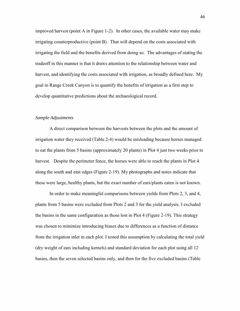
46
improved harvest (point A in Figure 1-2). In other cases, the available water may make
irrigating counterproductive (point B). That will depend on the costs associated with
irrigating the field and the benefits derived from doing so. The advantages of stating the
tradeoff in this manner is that it draws attention to the relationship between water and
harvest, and identifying the costs associated with irrigation, as broadly defined here. My
goal in Range Creek Canyon is to quantify the benefits of irrigation as a first step to
develop quantitative predictions about the archaeological record.
Sample Adjustments
A direct comparison between the harvests between the plots and the amount of
irrigation water they received (Table 2-4) would be misleading because horses managed
to eat the plants from 5 basins (approximately 20 plants) in Plot 4 just two weeks prior to
harvest. Despite the perimeter fence, the horses were able to reach the plants in Plot 4
along the south and east edges (Figure 2-19). My photographs and notes indicate that
these were large, healthy plants, but the exact number of ears/plants eaten is not known.
In order to make meaningful comparisons between yields from Plots 2, 3, and 4,
plants from 5 basins were excluded from Plots 2 and 3 for the yield analysis. I excluded
the basins in the same configuration as those lost in Plot 4 (Figure 2-19). This strategy
was chosen to minimize introducing biases due to differences as a function of distance
from the irrigation inlet in each plot. I tested this assumption by calculating the total yield
(dry weight of ears including kernels) and standard deviation for each plot using all 12
basins, then the seven selected basins only, and then for the five excluded basins (Table

47
2-5). Comparing the means and standard deviations of the entire plot to the areas that
were excluded demonstrated that this strategy was not biasing the results of my analysis.
Table 2-6 shows the total ear and grain weights for the subsample. Plot 1 received
only 7.37 cm (2.9 in) of precipitation during the growing season and all the corn died
before reaching maturity. Plot 2 was irrigated eight times (roughly once every two weeks)
and produced 1,257 g of edible kernels. Plot 3 was irrigated 12 times during the growing
season (roughly once per week) and had an edible grain yield of 1,358 g. The yield from
Plot 4 was 1,775 g after being irrigated 18 times (roughly two irrigation events per week)
during the growing season (Table 2-6).
These numbers were used to construct the graph illustrated in Figure 2-20. Note
that I assumed that the lack of any water, including from precipitation, would also have
produced no harvest. Comparing this graph with the expectations presented in Figure 1-2
provides some interesting insights. First, some amount of moisture is required for maize
to produce edible ears. In Range Creek Canyon, in 2014, the amount of that moisture
was greater than the 2.9 in of precipitation received during the growing season. Second,
there is a clear increase in the resulting harvests from adding increasingly greater
amounts of irrigation water to the fields across the irrigation schedules used in the
experiment. Last, we apparently did not reached the point of diminishing returns for
irrigating the fields; Figure 2-20 does not demonstrate the flattening of the curve
anticipated in Figure 1-2. Even more frequent irrigation, say three times or four times a
week, will be required to document the section of the relationship between water and
crop yield.

48
The yield clearly increases with increased available water. In this experiment,
increased water increased the overall ear weight per plot (in the sample), higher average
ear weight, greater mean ear and kernel weights, and increased health of ears in Plot 4
compared to the other plots based on gross morphology. Increasing the number of
irrigation events between Plots 3 and 4 by four produced significantly higher weight in
yield.
In future experiments I plan to spread the irrigation events out even further to fill
in the part of the curve between Plot 1 and Plot 2 to understand the absolute minimum
amount of irrigation required to produce edible yields in Range Creek under modern
conditions. But the trend is still clear; more water increases yield within the range
employed in 2014.
These findings are consistent with other farming experiments where water
(precipitation or irrigation) was a variable of interest (Adams et al. 1999; Denmead and
Shaw 1960; Garcia y Garcia et al. 2014; Hunt et al. 2014; Muenchrath 1995; Musick and
Dusek 1980; Robins and Domingo 1953). For example, in an early maize farming
experiment by Denmead and Shaw (1960), corn plants were raised in buckets and amount
of water was controlled on a schedule that stressed plants during three growth stages: 1)
vegetative, 2) reproductive, and 3) ear development. Of particularly importance was the
calculation of the interactions between stresses occurring at different stages. Simply
stated, the interactions explored whether plants that were moisture stressed at only one
stage produce more than plants that were stressed at more than one stage (Denmead and
Shaw 1960). Their results indicate that moisture stress during any one or more of the
growing stages reduced grain significantly, although the yield was most severely
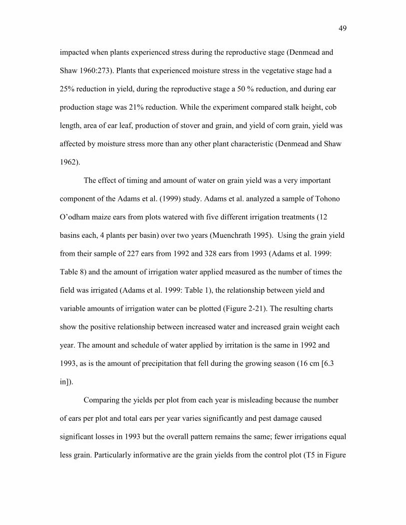
49
impacted when plants experienced stress during the reproductive stage (Denmead and
Shaw 1960:273). Plants that experienced moisture stress in the vegetative stage had a
25% reduction in yield, during the reproductive stage a 50 % reduction, and during ear
production stage was 21% reduction. While the experiment compared stalk height, cob
length, area of ear leaf, production of stover and grain, and yield of corn grain, yield was
affected by moisture stress more than any other plant characteristic (Denmead and Shaw
1962).
The effect of timing and amount of water on grain yield was a very important
component of the Adams et al. (1999) study. Adams et al. analyzed a sample of Tohono
O’odham maize ears from plots watered with five different irrigation treatments (12
basins each, 4 plants per basin) over two years (Muenchrath 1995). Using the grain yield
from their sample of 227 ears from 1992 and 328 ears from 1993 (Adams et al. 1999:
Table 8) and the amount of irrigation water applied measured as the number of times the
field was irrigated (Adams et al. 1999: Table 1), the relationship between yield and
variable amounts of irrigation water can be plotted (Figure 2-21). The resulting charts
show the positive relationship between increased water and increased grain weight each
year. The amount and schedule of water applied by irritation is the same in 1992 and
1993, as is the amount of precipitation that fell during the growing season (16 cm [6.3
in]).
Comparing the yields per plot from each year is misleading because the number
of ears per plot and total ears per year varies significantly and pest damage caused
significant losses in 1993 but the overall pattern remains the same; fewer irrigations equal
less grain. Particularly informative are the grain yields from the control plot (T5 in Figure

50
2-21) which was only irrigated once (at the time of planting). While not a complete loss,
the fields that did not receive additional irrigation water had significantly lower yield
compared to the fields that received one additional irrigation event (Treatment 4 and 5,
Adams et al. 1999: Table 8) during the growing season (a reduction of 44 % in 1992 and
73% yield reduction in 1993). Reduced returns from dry-land farming during dry years
would have significant impacts on the well being of prehistoric farmers (Adams et al.
1999; Adams et al. 2006).
Water and Yield Conclusions
Based on the results of the Range Creek experiment and many other studies of the
effects of water on yield, maize plants only produce edible grain when fields receive
enough water at planting and during a short window around the reproductive stage (about
4 weeks) (Adams et al. 1999; Denmead and Shaw 1960; Garcia y Garcia et al. 2014;
Hunt et al. 2014; Muenchrath 1995; Musick and Dusek 1980; Robins and Domingo 1953;
Andrade et al. 2000; Boyer and Westgate 2004; Claassen and Shaw 1970; Haegele 2008;
Saini and Westgate 2000; Setter et al. 2001). Additional water above this minimum
increases yields. Given the high yearly variation in rainfall amount and timing in the arid
west, the chances of receiving the necessary precipitation, at the right time, in the right
place, are low; probably often too low if it means the difference between making it
through the winter with enough to feed your family. If an investment in irrigation was not
made in advance of when the water was needed, then the loss to crops could be
substantial during a dry year.

51
If there is no source of irrigation water and the needs of the maize crop are not
being met by precipitation alone, a choice must be made: continue to try and farm, move
to an area with access to surface water or greater growing season precipitation, or switch
entirely to foraging (Barlow 2002). If irrigation is an option, then a farmer can decide if
the increased yield from having irrigation water available, when it is needed, is worth the
cost. Once a farmer has invested in irrigation to provide critical moisture during the
roughly 4 weeks around the reproductive phase, there are essentially no additional costs
for using the irrigation system repeatedly over the entire season. The payoffs for
irrigation only increase with use, within reason. The yields increase from the
supplemental water during the entire growing season but once initial costs of constructing
the irrigation system have been incurred, the costs of using that system are comparatively
small.
In Range Creek Canyon the costs of irrigation will be evaluated in the next phase
of the experiment (see Chapter 5), but it is clear that there were significant benefits to
irrigating in terms of increased harvest yield. The price of not providing supplemntal
water in the Range Creek experiment would have been no harvest, an outcome that many
farmers might not be able to overcome if alternative subsistence options are poor.
Because precipitation alone was not enough to water these plots at critical stages of
growth, an irrigation strategy designed to supply water often, for shorter periods of time
would be ideal for this shallow rooted variety growing in loamy sand.

Table 2-1
Comparison of Maize Farming Experiments 2013 and 2014
2013
Maize variety Location Field/plot layout Irrigation schedule Comments
Onaveño-120 day growing season, popcorn variety traditionally grown in Sonora Mexico.
Located 1 mile north of the Field Station Headquarters
4 plots Plot 1-not irrigated New shoots eaten by rabbits, continued to grow late into October but most ears did not reach full maturity
9 basins per plot Plot 2-irrigated 1 x per week 5 seeds per basin Plot 3-irrigated 2 x per week
Plot 4-irrigated as needed
2014
Tohono O'odham "60 day"- 80-100 day growing season, flour variety traditionally grown in Southern Arizona and Northern Mexico.
Located at the Field Station Headquarters
4 plots Plot 1-not irrigated Rabbit proof fence used early, shorter growing season, most ears reached full maturity
12 basins per plot
Plot 2-irrigated 1 x every 2 weeks
5 seeds per basin Plot 3-irrigated 1 x per week
Plot 4-irrigated 2 x per week
52

53
Figure 2-1. Contour map of the Range Creek Field Station headquarters showing the location of the 2014 experimental maize plots.

54
Figure 2-2. Overview of the experimental maize crop facing north on planting day, May 20, 2014. Plots are located in the former orchard of the Range Creek Field Station
headquarters.
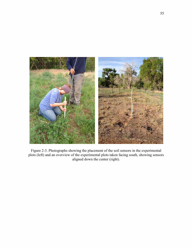
55
Figure 2-3. Photographs showing the placement of the soil sensors in the experimental plots (left) and an overview of the experimental plots taken facing south, showing sensors
aligned down the center (right).

56
Figure 2-4. Photographs showing the placement of the soil sensors in the control plot (left) and the application of water to the control plot (right).

57
Figure 2-5. Chart showing soil moisture data for the sensor control plot. Data are from four sensors, placed at 6 in (6c, blue line), 12 in (12c, red line), 24 in (24c, the green
line), and 36 in (36c, black line) below ground surface. Black arrows indicate the dates that water was added to the plot and the amount in gallons. Blue vertical sections indicate
timing and amount of precipitation received.

58
Table 2-2
Precipitation at the Experimental Plots during the Growing Season
Date Precipitation (in/cm) Comments
July 9, 2014 0.13/0.33
July 28, 2014 0.18/0.46
August 03, 2014 1.57/4.0 over 3 days
August 21, 2014 0.49/1.24
August 27, 2014 0.53/1.35 over 3 days

59
Figure 2-6. Overview photograph showing Plot 1. Plot 1 was irrigated only once, on the day it was planted. The Plot 1 plants dried up and died shortly after June 16, 2014.

Figure 2-7. Chart showing soil moisture sensor data from Plot 2. Data are from two sensors placed at 12 in (12e, black line) and 30 in (30e, red line) below ground surface. Vertical arrows indicate irrigation events. Plot 2 was irrigated 8 times during the growing season
(irrigation event on planting day May 20, 2014 not shown). Blue sections indicate timing and amount of precipitation received. The red area is the timing of critical reproductive stage. The sun symbol indicates the first recorded tassels.
60

Figure 2-8. Photographs taken on July 23, 2014, showing maize plants from experimental farm plots. Example of plants in Plot 2, showing stunted growth and severe water stress between irrigation events (top center). Example of plants in Plot 4 (bottom right) on
the same day show healthier and vigorous foliage.
61

Figure 2-9. Photographs showing maize plants from Plot 4. (Left) These three plants were excavated from a single basin to examine rooting depth at the end of the growing season. (Right) Note the shallow affective root zone, only 25 cm (10 in) below surface
including tap roots.
62

63
Figure 2-10. Chart showing soil moisture sensor data from Plot 3. Vertical arrows indicate irrigation events. Plot 3 was irrigated 10 times during the growing season
(irrigation event on planting day May 20, 2014 not shown). Blue sections indicate timing and amount of precipitation received. The red area is the timing of critical reproductive
stage. The sun symbol indicates the first tasseling recorded.

64
Figure 2-11. Chart showing soil moisture sensor data from Plot 4. Vertical arrows indicate irrigation events. Plot 4 was irrigated 14 times during the growing season (first irrigation event on planting day May 20, 2014 not shown). Blue sections indicate timing and amount of precipitation received. The red area is the timing of critical reproductive
stage. The sun symbol indicates the first recorded tasseling.

65
Figure 2-12. Overview of experimental farm plots.

66
Figure 2-13. Photographs showing overview of a basin and a close up of cobs prior to harvest.

67
Table 2-3
Summary of Yields from Experimental Plots in 2013 and 2014.
plot no. total basins
seeds planted
total plants
mean plant ht.
(cm)
total mature
ears
2013 (Onaveño)
1 9 45 7 33 0
2 9 45 32 201 5
3 9 49 40 215 7
4 9 45 36 217 7
total 36 184 115 167 19
2014 (Tohono O’odham)
1 12 60 0 0 0
2 12 60 56 137 58
3 12 60 58 150 60
4* 12 60 41 166 38
total 48 240 155 151 156 *Plants in 5 of 12 basins were lost to horse damage; totals are for those basins not damaged by horses and several ears recovered from damaged plants.

Table 2-4
Results of Ear Descriptive Analysis
plot no.
total ears
ear wt. (g) x̅/s
ear length (mm)
x̅/s
ear diameter
(mm) x̅/s
mean % kernel
coverage
grain wt. per ear (g)
x̅/s
total ear wt. (g)
total edible grain
wt. (g)
total irrigation
events
no. of ears with stress indicators
1 0 0 0 0 0 0 0 0 1 0
2 58 38.5/24.7 130/37 28/4 75 30.3/21.5 2,158 1,732 8 34
3 60 48.1/23.6 146/31 30/4 80 40.0/20.6 2,888 2,400 12 33
4 38 60.4/40.4 158/51 29/6 80 50.5/34.6 2,295 1,916 18 11
total 156 48.0 144 29/5 80 38.9/26.0 7,341 6,048 39 78
68

Figure 2-14. Selection of ears from irrigated experimental plots. (a) Plot 2, (b) Plot 3, (c) Plot 4.
A A A
B B B
C C
A
69

70
Figure 2-15. Examples of undeveloped kernels on tips of ears. Mean percentage of kernel coverage is reported in Table 2-3.

71
Figure 2-16. Example of patchy kernel development along the length of the ear. Patchy kernel development is a morphological characteristic likely associated with
environmental stress that occurred more often in Plots 2 and 3.

72
Figure 2-17. Two examples of ears with irregular rows, a morphological characteristic likely associated with environmental stress, was more common in Plots 2 and 3.

73
Figure 2-18. Photographs of ears showing pink discoloration.

74
Figure 2-19. Map showing the location of horse damaged basins in Plot 4 and the location of basins selected for exclusion from Plots 2 and 3.

75
Table 2-5
Descriptive Summary of Plot 2 and Plot 3 Yield.
Plot no./basins total ear wt. (g)
ear wt. (g) x̅/s
total grain wt. (g)
grain wt./ear(g)
x̅/s
Plot 2 12 basins 2159 38.5/18.1 1,733 31.0/16.4
7 basins in sample 1528 48.0/17.0 1,257 39.6/15.3
5 excluded basins 631 25.2/9.4 475 19.0/8.6
Plot 3 12 basins 2888 48.1/8.5 2,401 40.0/7.8
7 basins in sample 1641 48.1/9.3 1,358 39.8/8.3
5 excluded basins 1247 48.1/8.7 1,043 40.2/8.0

76
Table 2-6
Descriptive Summary of Yield Samples
plot no. no. mature
ears in sample
ear wt. (g) in sample
edible grain wt. (g) in sample
total irrigation
events
2 33 1,528 1,257 8
3 34 1,641 1,358 12
4 35 2,133 1,775 18

77
Figure 2-20. Graph showing increase in total grain yield as number of irrigations increase. All plots received 7.37 cm (2.9 in) of rain during the growing season. The data
points between plots were estimated using the surrounding data points.

Figure 2-21. Results of maize farming experiment showing total amount of grain yield (g) and amount of irrigation water applied (number of days) for two growing seasons (Adams et al. 1999: Table 1 and Table 8). Data points are labeled using water treatment
numbers from Adams et al. 1999. The slope between irrigation events 5-7 is estimated using the total yield from T2 and T1.
78
CHAPTER 3
ENVIRONMENTAL CONSTRAINTS ON FARMING
The success of farming is largely conditioned by a number of physical variables,
as well as an investment of time and energy on the part of farmers. “Year to year
variability in either precipitation or length of growing season can be large and can be the
deciding factor between success and failure in crop production” (Petersen 1985:37). One
emphasis of my research is that success is a relative term: great success under one set of
circumstances might well be viewed as marginal success under other circumstances. The
key to understanding prehistoric farming is to understand it as a process of sequential
activities, ranging from choosing where to farm, field preparation, planting, tending, and
harvesting. Choice of field location is likely to be a function of the availability of land
with various soils, slopes and aspects, distance to surface water, etc. This will be both a
function of natural availability and what other fields are already in place at the time the
choice is made. As the population in Range Creek Canyon increased over time, the
social constraints on choice of location likely became more important, and the
environmental constraints became less important.
In this chapter, I consider four variables of the physical environment that are
important to the success of farming in a specific plot in Range Creek Canyon:
precipitation, seasonality of temperature (measured as both frost free season and

80
cumulative growing degree days), contiguous arable land (on the valley floor, relatively
close to the creek, and less than a 12 degree slope), and soil texture. Unlike the last two
variables, arable land and soil texture, temperature and precipitation fluctuate at a variety
of time scales: days and months, years and decades, and centuries. My goal in this
chapter is to characterize each variable with existing data across the canyon bottom of
Range Creek. The emphasis is to identify, quantify, and model the spatial variation in
these variables as the first step in identifying how that variation is likely to combine to
influence the success of farming in the canyon today. This will then serve as the context
to explore how longer-term climatic changes might have affected the options available to
the prehistoric populations who farmed in this canyon 1,000 to 800 years ago; more
specifically, how climatic fluctuations influenced the costs and benefits of farming in this
rugged region of central Utah.
Precipitation To understand the relationship between water and harvest yield, it is important to
first define two concepts for scaling farming success. First is the “maximum harvest” or
the amount of food harvested without attention to the costs associated with farming. This
is a theoretical yield that is unlikely to ever be observed and is only useful as a context
for discussing variation in the second concept, “optimal harvest.”
Optimal harvest takes into account the costs associated with improving the yield.
The costs include both capital investments and maintenance costs associated with
planting, weeding, irrigating, field preparation, etc. The optimal harvest is the value that
factors in real-life limitations of a specific time and place, and will be a function of

81
terrain, soil, precipitation, access to surface water, technology, etc. In other words, the
variation seen among modern farmers, or what has been recorded for historic farmers, is
variation in the optimal harvest.
This study is particularly focused on measuring optimal harvest and the costs and
benefits of irrigation. If there is enough available water from precipitation to produce a
harvest but the harvest could still improve with more water, then irrigation will optimize
the yield if the costs of irrigation are less than the benefit of the additional harvest. On the
other hand, if there is plenty of naturally available water for a productive harvest then
irrigation may not be profitable. Before reconstructing the past productivity of Fremont
farmers, the commonly used precipitation thresholds must be evaluated in the modern
and historic environment to understand their effects on maize farming today.
I use three measures of precipitation at various scales and time frames to measure
available water in Range Creek Canyon. The first precipitation dataset comes from the
two largely automated weather stations located at the Field Station. The second data set
was compiled from a series of manual rain gauges placed along the canyon floor. The
third precipitation dataset is from the PRISM Climate Group at Oregon State University.
Weather Stations
Precipitation data were collected in Range Creek Canyon by weather stations in
two locations (Figure 3-1). The location closest to the experimental farm field (Weather
Station 1) has been collecting data since the fall of 2008. A faulty sensor (and a
maintenance error) resulted in only partial precipitation data collection for parts of 2010-
2011, and 2013, 2014. Weather Station 2, located near the northern boundary of the Field

82
Station, was installed in the summer of 2013. Both weather stations use ETI NOAH II
precipitation gauges attached to Campbell Scientific CR1000 data loggers. Fifteen-
minute and one-hour summary files are maintained by the data loggers, allowing fine
grained comparison of precipitation at the two sites and a precise accounting of
precipitation during the growing season.
Rain Gauges
Eleven manual rain gauges were spaced north to south along the valley floor of
the Range Creek Field Station (Figure 3-1) in 2013. The manual rain gauges used are
CoCoRaHS Rain & Snow Gauges that have a precision of 0.01 in and a maximum
capacity of 12 in of precipitation. A thin layer of mineral oil was added to the catch tube
of each of the gauges to minimize evaporation between the rain event and the time of data
collection. For two years, the amount of precipitation captured by each of these gauges
has been recorded for major precipitation events that occurred between May and
November. Samples of the rain water were also collected for isotope analysis. During
the 2014 growing season, the rain gauge located at the Field Station Headquarters, where
the experimental crop was grown, was the primary measure of precipitation for the
farming experiment.
PRISM Climate Data
For a reconstruction of precipitation over a longer period, I used datasets available
online from the PRISM Climate Group website (http://www.prism.oregonstate.edu/).
These climate datasets are used by thousands of agencies, universities, and companies to

83
assist in agronomy, engineering, hydrology, ecology, and natural resource conservation
projects (Daly et al. 2008). PRISM stands for Parameter-elevation Relationships on
Independent Slopes Model (Daly et al. 2008). The model creates a gridded (raster)
dataset of precipitation and temperature, available in digital form, interpolated from
Digital Elevation Models (DEM) and weather station data points (n = ~13,000 stations
for precipitation and n = ~10,000 stations for temperature). Since weather stations are not
available at every grid cell of a DEM, those used in the model are assigned weights based
on physiographic similarity between the station and the nearby grid cell, and a climate-
elevation regression is calculated factoring in a variety of topographic features (Daly et
al. 2008).
The algorithm was designed to mimic the process a climatologist goes through
when they draw a climate map and uses attributes including location, elevation, and
terrain. While precipitation and temperature are closely linked to and often determined by
elevation, there is considerable variation across the landscape (Daly and Bryant 2013).
By dividing the terrain into “facets” with multiple slope orientations, weather stations
located within these same orientation categories are assigned a “facet.” Thus, only
weather stations within the same terrain characteristics as the grid cell of interest are used
in the calculation of the cell’s precipitation and temperature value, creating a local
statistical relationship not often included in such broad scale climate analyses (Daly and
Bryant 2013). The model uses the same methods to control for proximity to coastlines,
location of temperature inversions and cold air pools, and many other complex variables
which are most important at scales from less than 1 km to 50 km (Daly et al. 2008). The

84
datasets generated represent the current state of knowledge of spatial climate patterns in
the United States (Daly et al. 2008).
Prism estimates were available for reconstructing monthly precipitation for the
past 30 years in Range Creek Canyon and provide the basis for exploring the spatial
extent of the often cited thresholds necessary for dry maize farming. I downloaded
PRISM datasets containing the 30-year precipitation values from 1981-2010. From these
files, I created three raster data sets for comparison: one for annual precipitation, one for
summer months only (June-September), and one for the winter (October-March). I
generated contour maps for the average available precipitation for summer, winter, and
the entire year to identify how these varied across Range Creek Canyon. This method
provides a reasonable estimate of variation in the ”value” of farm land within Range
Creek Canyon in the context of dry farming and precipitation
Precipitation--Results
When studying prehistoric farmers, archaeologists often ask whether dry farming
was possible in the area under consideration. In some cases this makes perfect sense: if
there was no source of reliable surface water for irrigation, then surface irrigation was not
an option to the prehistoric farmers. But if a water source is available, then the better
question is whether the benefits of increased harvests with irrigation outweigh the capital
and maintenance costs of irrigating. When the net gain is positive, then irrigation should
be considered to be a viable option; when negative, irrigation is not expected.
Annual precipitation on the Colorado Plateau, and actually over large areas of
western North America, is largely a function of elevation, among other variables. All

85
else equal, higher elevations receive more precipitation than lower elevations. For
farmers, especially farmers without a source of reliable surface water, moving to higher
elevations increases the likelihood of a successful season of farming. Of course,
temperature also fluctuates with elevation; higher elevations have cooler temperatures
and therefore shorter frost-free seasons and lower growing degree days, which also
influence farming productivity. Many authors have investigated settlement patterns in
terms of the tradeoff between water and temperature as a function of elevation (e.g.,
Adams 2004; Adams and Petersen 1999; Barlow 2002; Benson and Berry 2009; Janetski
et al. 2012; Netting 1972; Petersen et al. 1985; Petersen 1994; Van West 1994).
Thresholds for Dry Farming
To evaluate the benefits of supplemental irrigation water on corn production, it is
important to document the amount of precipitation available along the length of Range
Creek Canyon. The typical rule of thumb for dry maize farming is that at least 30 cm (12
in) of annual precipitation is necessary with at least 15 cm (6 in) of that coming during
the growing season (Benson et al. 2013; Benson 2010a; Benson and Berry 2009; Shaw
1988). While these are generally cited as the minimum thresholds for dry farming, it is
also recognized that water stress is likely when precipitation below 40 cm (16 in) is
available during the summer, and that healthy maize crops in the Corn Belt normally
require between 41 and 64 cm (16-25 in) during the growing season (Benson et al. 2013;
Hanway 1966:p158). For the evaluation of Range Creek Canyon the thresholds used for
annual precipitation are: < 30 cm (12 in, inadequate), 30 (adequate) and > 50 cm (20 in,
healthy). The majority of that annual precipitation needs to fall between June and July to

86
meet the following summer precipitation requirements: 15 cm (6 in, lower limits), 20 cm
(8 in, stressed), and 40 cm (16 in, healthy).
Winter precipitation is also essential because it is often the source of soil moisture
required at the time of planting for germination and plant growth through emergence.
While there does not appear to be a reported standard threshold for the amount of winter
precipitation necessary for productive maize farming, I assume that the annual threshold
minus the summer threshold is a fair estimate of the amount of winter precipitation
necessary for dry-land farming. For example if 30 cm (12 in) annual precipitation is
adequate for dry farming maize, and 15 cm (6 in) of that amount is required during the
growing season, then that leaves 15 cm (6 in) falling during the winter. For irrigation-
based farming strategies, the higher the winter precipitation amount, the better since it is
often the principal source of available surface water. A winter threshold estimate of 5 cm
(2 in, inadequate), 10 cm (4 in, stressed), and >10 cm (> 4 in, adequate) is used to
evaluate the winter precipitation estimates for the last 30 years in Range Creek Canyon.
Recent Precipitation Variability in Range Creek Canyon
Before evaluating the effect of variability in precipitation on farming yield and
behavioral responses during the prehistoric occupation of Range Creek, it is important to
understand how variability in the modern record of precipitation affects maize yields and
decisions about field location. This baseline understanding of the present pattern of
available water will serve as the context against which to explore how longer term
changes in water availability may have affected the options available to the prehistoric

87
farmers in this canyon 1,000 to 800 years ago; more specifically, how fluctuations in
precipitation influenced the costs and benefits of farming in Range Creek Canyon.
Weather station record. We have a six-year sample of precipitation data available
from Weather Station 1. While this sample size is small it clearly demonstrates the
variability in monthly and yearly precipitation available in the canyon. While mean
annual precipitation over many years can show the general trend in available moisture for
an area, the success of a dry farmed maize crop depends not only on the amount of
rainfall in a single year, but also on the timing of that rainfall. To evaluate the trend in
growing season precipitation over the last six years I recorded the high, low, and mean
monthly precipitation values for the last six years in Range Creek Canyon from Weather
Station 1 (Figures 2-1 & 2-2). The range of values for precipitation received per month
over the last six years has varied substantially.
The widest range of values was evident in the September data set, with a low of
0.99 cm (0.39 in) in 2010 and a high in 2013 of 9.14 cm (3.6 in). What is especially
interesting is that even with this range of variability, there has been only one year wet
enough to reach above the 20 cm (8 in) precipitation threshold (stressed) during the
growing season. Even during the wettest growing season (2013) with a total precipitation
value of 10.49 in (26.64 cm) between May and October, over half the total value fell
within September/October (Figure 3-3). The 6.8 cm (2.7 in) that fell between July and
August of 2013 (the critical reproductive stage for kernel development) would have
inflicted considerable stress on the crop. The take away message for farming with the
recent precipitation pattern in Range Creek Canyon is that there is high month to month
and year to year variability with overall low available moisture between June and August.

88
Equally important, this estimate of variance undoubtedly underestimates the true
variability that would be evident in a 30-year span, let alone a 300-year or 2,000-year
span. More complete years of data collection in the future will undoubtedly refine this
pattern.
Weather Station 1 provides only one data point near the center of the canyon to
estimate the precipitation values for the surrounding farmland. The amount that actually
falls on any given piece of land nearby is only an estimate. We know from time spent in
the canyon that one needs only drive around the next bend in the road to get out of the
rain from a summer storm. Weather Station 2 helps capture this variability at a finer
resolution and provide data for comparisons of precipitation and elevation. We expect the
amount of precipitation to increase with increased elevation but with only six years of
data from the center of the canyon and one year from the northern boundary of the field
station, that pattern is not yet visible from weather station data alone. Manual rain gauges
are used to supplement the weather station precipitation data.
Rain gauges. Precipitation totals from 10 rain gauges in 2013 and an 11th gauge
added in 2014 are reported in Table 3-1. We only have records from May through
December because the field station is closed during the late winter and early spring. The
rain gauge (RG) numbers correspond to the numbered points illustrated in Figure 3-1 and
show the range of variability in different sections of the canyon over these two years. As
expected, the general trend in the total yearly precipitation is a decrease from higher (RG-
1) to lower (RG-11) elevations (Figure 3-4). These data allow us to measure the timing
and intensity of rain events during the growing season. We had anticipated comparing
that data with the rainfall recorded at Weather Station 1, located just north of the

89
experiment but the 2014 precipitation data was lost due to a malfunctioning sensor. The
experimental plots received 2.9 in (7.73 cm) of precipitation that fell over nine days
during the growing season (May-August) as measured by RG-10. Clearly the thresholds
for adequate precipitation for dry farming were not met. The impacts of available
moisture on the experimental maize harvests were discussed in Chapter 2.
Regional Precipitation Variability in Range Creek Canyon
PRISM Climate Group offer 30 years of climate data, with estimates of
precipitation, minimum temperature, maximum temperature, and dew point. The
following figures are calculated from PRISM data sets from 1981-2010 at 800 m
resolution (for convenience, I will refer to this as the “last 30 years”). Figure 3-5 shows
the average annual rainfall over this period in Range Creek Canyon. It estimates the
geographic limits to productive dry farming, with > 30 cm (≥ 12 in) of precipitation,
requires farming at elevations greater than about 1,765 m (5,790 ft).
Examining just the rainfall during the growing season, from June through
September, demonstrates that the 15 cm (6 in) precipitation, conventionally viewed as the
minimum for dry farming, is located slightly above 2,120 m (6,950 ft) in elevation, more
than 350 m higher than the threshold calculated based on annual rainfall (Figure 3-6). As
I will show later, this elevation is pushing the limits of having sufficient growing season
temperatures needed for corn to reach maturity.
My estimate of a minimum of 10 cm (4 in) of precipitation from November
through March is, on average, available on the canyon floor at or above 1,750 m (5,740
ft) in elevation, well south of the elevation threshold for adequate summer precipitation

90
(Figure 3-7). Any increases in precipitation at higher elevations during the winter would
increase the run-off into Range Creek directly influencing the amount of irrigation water
available at lower elevations. In Range Creek Canyon, growing season precipitation is
the limiting variable.
The map of growing season precipitation (Figure 3-6) is based on the average
monthly precipitation, but obviously some years had more rainfall than others. I therefore
modeled the variance in monthly rainfall by elevation. Figure 3-8 illustrates the mean
and variance of growing season precipitation modeled as normal distributions for
increments of 1,000 ft (300 m) of elevation based on the PRISM precipitation data. The
vertical line indicates 15 cm (6 in). The portions of the distributions to the right of that
line are the probabilities of receiving 15 cm (6 in) or more precipitation. Even at 9,000 ft
(2,700 m) in elevation, there is only about a 30% chance of receiving 15 cm (6 in) or
more precipitation during the growing season, and that probability decreases at lower
elevations. As discussed below, it is impossible to farm at 9,000 ft (2,700 m) because of
the low seasonal temperatures.
Seasonality of Temperature in Range Creek Canyon
Daily temperatures are also a critical constraint on the success of farming. Spatial
variability in temperatures, in regions with significant topographic relief, during the
growing season will be another determinant of when and where various maize varieties
are likely to be successful, as well as the size of the resulting harvest. Plant growth and
development are dependent on temperature, as well as available moisture. Warmer
temperatures encourage more rapid development and cooler temperatures can slow down

91
or halt development (Neild and Newman 1990). Corn plants not only require a sufficient
number above freezing days to develop, but the rate of maturation is strongly conditioned
by temperature. The measure of temperatures accumulated over time is calculated in heat
units or Growing Degree Days (GDD). Each maize variety has a threshold of
accumulated heat units or GDD that must be reached within the growing season for corn
to attain physiological maturity.
Temperature
The length of a growing season is directly tied to temperature which changes
systematically with elevation (Daly et al. 2008; Neild and Newman 1990). In Range
Creek Canyon, temperature data are available from two automated weather stations
(Figure 3-1), with a difference in elevation of 370 m (1,210 ft). Using the daily difference
in temperature between these two locations, I was able to estimate the growing season at
any elevation in the canyon.
The scales used to measure growing season here are Frost Free Days (FFD) and
Growing Degree Days (GDD). Frost Free Days are the number of days between freezing
temperatures in the spring and fall (Neild and Newman 1990). This is the number of days
available for the corn plants to progress through the growth stages of germination,
reproduction, and maturity. During the frost free period, the rate of maize maturation is
determined by accumulated heat units measured in Growing Degree Days (GDD).
Frost Free Days (FFD). The period between the last spring frost and the first frost
in the fall is generally considered the growing season (Neild and Newman 1990). Frost
Free Days (FFD) can be counted by identifying the last day that temperatures reached 32
92
°F (0 °C) or below in the spring and the first date that the temperature dips to 32 °F (0
°C) or below in the fall. FFD was calculated using data collected from weather stations in
two locations (Figure 3-1). The location closest to the experimental farm field (Weather
Station 1) has been collecting data since the summer of 2008 for a total of six complete
growing seasons. Weather Station 2, located in the northern boundary of the Field
Station, has been recording data since the summer of 2013 which means only one
complete growing season and a little over half of another growing season available for
analysis of higher elevations. Temperature data were analyzed to calculate the FFD for
each complete growing season, to compare the change in FFD over the 370 m (1,210 ft)
elevation difference between weather stations.
Growing Degree Days (GDD). Developmental growth stages in most plants are
linked to the number of heat units or GDD that are accumulated during the growing
season (see Adams et al. 2006; Benson et al. 2013; McMaster and Wilhelm 1997;
Muenchrath 1995; Muenchrath and Salvador 1995; Neild and Newman 1990 for further
discussion of GDD). There are temperature thresholds above and below which certain
plants cannot grow or they experience stress. GDD is calculated by subtracting the
temperature base (50 °F for maize) from the average daily temperature, represented by
the following equation:
GDD = (Tmax + Tmin)/2 - Tbase
Tmax is the maximum temperature on a particular day during the growing season, and Tmin
is the minimum temperature for that day. Because modern corn hybrids exhibit little or
no growth at temperatures below 50 °F, Tmin and Tmax are set to 50 °F when the actual
daily temperature extremes are < 50 °F. Similarly, there is little increase in growth at

93
temperatures above 86° F and consequently Tmax is set to 860 F when the maximum
temperature exceeds 86 °F (30 °C). When neither the minimum or maximum
temperatures exceed 50 °F, then the GDD for that day is 0. When Tmin equals 45 °F, and
Tmax equals 78 °F, GDD = (50+ 78)/2-50 = 14. The maximum GDD is 36 when neither
Tmin and Tmax drops below 86 °F.
A measure of Cumulative Growing Degree Days (CGDD) is calculated by
summing the daily GDD values starting from the date of planting to the end of the
growing season. All CGDD measures here are calculated in degrees Fahrenheit and
CGDD reported by other studies in degrees Celsius are converted to degrees Fahrenheit
for comparison. CGDD was calculated for Range Creek using six years of temperature
data from Weather Station 1 and the one year of available data from Weather Station 2.
Using the difference in elevation between these two weather stations, the change in daily
temperature as a function of elevation was calculated and used to make estimates of
CGDD for arable land along the elevation gradient of the canyon floor. The planting date
used for CGDD estimates closer to Weather Station 1 is May 8th, the latest spring freeze
at Weather Station 1 over the full six years. The planting date used for CGDD estimates
closer to Weather Station 2 was May 16th, the latest spring freeze recorded at that
elevation.
Modern corn hybrids require 2700 CGDD to reach maturity during the growing
season (Neild and Newman 1990) and most dry adapted land races require fewer. If the
needed CGDD is not reached before the first freezing temperatures in the fall, maize ears
will not reach full maturity. The CGDD of the experimental Tohono O’odham maize crop
grown in Range Creek Canyon was compared to the 2700 CGDD average for modern

94
hybrids and will be compared to the results from other experiments where dry adapted
land races were grown. The modern record of temperature variation and its constraints on
farming success in Range Creek Canyon is discussed below and will be used to make
predictions about how yearly variation in temperature and growing season might have
influenced prehistoric farming success in Chapter 4.
Growing Season--Results
Prehistoric farmers could not predict or control daily or yearly variation in
temperature that affected their harvest, but they should have preferred field locations that
minimize the risk of reduced harvests due to cooler temperatures. Increasing elevation is
directly linked to decreasing temperature, so choosing a farm location at a lower
elevation can increase the chances of reaching the necessary CGDD before the first fall
freeze. But it is not as simple as moving as far south in the canyon as possible. Locating
farm fields at lower elevations comes with its own costs, such as decreased precipitation
and temperatures that are too high for optimal growth, as well as a deficit in surface water
available for irrigation because neighbors upstream are diverting it into their fields. Only
the first farmers get to choose the optimal locations without reference to existing farm
fields.
Given these tradeoffs, the question is more about how the various constraints
combine to determine the value of land for farming along the length of the canyon floor
of Range Creek Canyon. I will discuss the FFD and CGDD for the experimental maize
crop grown in 2014 at (1,500 m) elevation. Using that example, I will generate a model
for where farming is more or less successful given the FFD and CGDD at increasing

95
elevations in the canyon. I will present an example showing how variation in temperature
over just two growing seasons can affect yields depending on field location.
Frost Free Days (FFD)
The Frost Free Days (FFD) were calculated using data collected from the weather
stations (Figure 3-1). The data on the frost free growing season for each year are
summarized by weather station (Table 3-2). For Weather Station 1, the mean FFD for six
years with complete records is 169 days with a range from 154 to 194 days. Weather
Station 2 had 139 FFD days in 2014, or 30 days less than the average for Weather Station
1 and 40 days less than the 2014 readings from Weather Station 1. These differences are
principally the consequence of the 370 m (1,210 ft) difference in elevation between the
two weather stations. Based solely on FFD, locating farm fields more centrally in the
canyon reduces the risk of freezing temperatures hitting crops before they are mature. On
average, crops can be planted earlier and harvested later around Weather Station 1.
Experimental Crop CGDD
The Cumulative Growing Degree Days (CGDD) was calculated for the 2014
growing season to track the growth stages of the experimental crop. The starting date
used was the planting date, May 20, 2014. Table 3-3 shows the CGDD requirements for
different developmental stages for a 2700 CGDD hybrid (Neild and Newman 1991). The
growth stages of Tohono O’odham maize followed the average CGDD requirements for
hybrid field corn maturity quite closely until the reproductive stage was reached; then
ears in the experimental plots reached maturity more quickly. While there was variation

96
within and between plots, the majority of the Tohono O’odham maize reached the
reproductive stage around 65 days after planting, with emerging tassels, fully emerged
tassels dropping pollen, and silks recorded in all three plots on July 23. The CGDD on
July 23 was 1419 which is the CGDD required for modern corn hybrids to reach this
reproductive stage (Table 3-3). Many ears had reached dough stage by August 19, with a
CGDD of 2027. This is the stage when the Tohono O’odham harvest some green ears
(immature milky kernels) for roasting while the remaining ears continue to mature to
their full weight and dry for storage (Castetter and Bell 19942; Muenchrath 1995).
The Range Creek experimental maize reached maturity between 2100 and 2400
CGDD. On August 29 it was noted that some ears appeared fully mature with a CGDD of
2177. Due to flooding damage to the dams, the fields were no longer irrigated after this
date. By September 10th, it was estimated that all ears had reached physiological maturity
at 114 days with a CGDD of 2400. Within a week, the weight of the ears began pulling
the dried stalks over and they were being eaten by pests and had to be collected for
further analysis. Due to logistical constraints, the ears remained on the stalks to dry until
September 23rd when all ears were harvested. Tests of the kernels in the lab showed black
layer formation indicating that the majority of ears had reached full maturity (Neilsen
2001, 2009).
Canyon-wide Estimates of CGDD
With the CGDD requirements for Tohono O’odham grown in Range Creek as a
baseline, I looked at how the same variety would fare growing at increased elevation and
during past years for which we have temperature data. CGDD was calculated for six

97
years of temperature data from Weather Station 1 (Figure 3-9). The planting date used
was the latest spring freeze date for all six years, May 8 (Table 3-2). Figure 3-9 shows all
six years had reached a CGDD of 2700 by 145 days after planting. By comparing the
average CGDD for all six years from Weather Station 1 to the temperatures at Weather
Station 2 in 2014, it is clear that with an increase of only 370 m (1,210 ft) in elevation
there is a significant difference in CGDD (Figure 3-10).
Using the difference in elevation and the difference in daily temperature over the
growing season between the two known points, I estimated the CGDD for five elevations
between the weather stations (Figure 3-11). The first fall freeze at Weather Station 2
(2,060 m [6,760 ft] elevation) was on October 01, 2014 which gives us a minimum FFD
for the other locations although they would have slightly longer FFD as elevation
decreases. Based on the results of the experimental farm plots, Tohono O’odham maize
reached physiological maturity at about 2400 CGDD. With the overall warmer 2014
temperatures, any maize fields planted at or below an elevation of 1,880 m (6,170 ft)
could have reached maturity with a CGDD of 2400 before the first fall freeze. Crops
planted between 2,060 m (6,760 ft) and 1,880 m (6,170 ft) elevation all reached a CGDD
of 2100 by the first freeze. Some of the ears in the experimental plot had reached
maturity by 2100 CGDD so planting at higher elevations during a warm year would not
have been a complete loss.
We only have one complete growing season from Weather Station 2 but we know
that there is considerable yearly variability in temperatures in Range Creek Canyon. For
example the second half of the 2013 growing season was considerably cooler than 2014. I
used the temperature data from August-October, 2013 to create a second estimate of the

98
CGDD temperatures during a cooler year to see how much the picture changed (Figure 3-
12). The first fall freeze changes by only a few days to September 27, 2013 but with the
overall cooler 2013 temperatures CGDD goes down significantly compared to 2014.
Maize fields planted at an elevation of 1,880 m (6,170 ft) would have barely reached a
CGDD of 2400 by the first freeze. Fields planted above 1,880 m (6,170 ft) and below
2,010 m (6,590 ft) might have produced some mature ears before the freeze. Crops
planted at an elevation above 2,010 m (6,590 ft) would have been unlikely to reach
maturity before the first freeze.
While this is a small sample of yearly data, it is clear that temperature variation
can have significant effects on maize development at very small spatial and short
temporal scales. The horizontal distance between the two weather stations is
approximately 11.5 km (7.15 miles) with a difference of 370 m (1,210 ft) elevation. The
location chosen to farm between those two points could lead to high yields in one year
and the next growing season a near loss based solely on temperature. Under current
climatic conditions, planting above 2,000 m (6,561 ft) would be risky in cooler years
(Figure 3-13). Planting well below 2,000 m (6,561 ft) would be ideal although
precipitation decreases with decrease in elevation. Irrigation is one strategy for dealing
with precipitation deficits while taking advantage of warmer temperatures at lower
elevations.
Regional Temperature Variability
Our local temperature data suffers from small sample size, limited in time and
space. At this point, it is safe to argue that the weather station data under represents the

99
annual variability in temperature if we were able to measure it over decades, and
certainly over centuries. Using daily minimum and maximum temperature data, modeled
from PRISM data, I was able to estimate the FFD and CGDD for the last 30 years at five
elevations in Range Creek Canyon. To determine the FFD for each year I downloaded the
daily minimum and maximum temperature values for March-November for each year,
1981-2010, at five elevations. I then recorded the last spring freeze and first fall freeze
for each year (≤ 32 ° F) and calculated the probability of reaching ≥120 FFD days at each
elevation over the last 30 years. I then used the same data set to calculate CGDD using
the formula described above starting with the day following the last spring freeze of that
year as the planting date. I calculated the probability of achieving ≥ 2250 CGDD at each
elevation.
Figure 3-14 illustrates the mean and variance of FFD and CGDD modeled as
normal distributions for increments of 1,000 ft (300 m) of elevation based on the PRISM
precipitation data. The vertical lines indicate the necessary FFD and CGDD
requirements for Tohono O’odham from the Range Creek farming experiment (120 FFD
and 2250 CGDD). The portions of the distributions to the right of that line are the
probabilities of receiving120 or more FFD and 2250 or more CGDD. Figure 3-15
compares the FFD and CGDD as proxies for growing season in Range Creek Canyon. It
is clear that while FFD sets the limits on the growing season, CGDD better approximates
the amount of heat available for maize growth within the frost free period. For example at
8,000 ft (2,450 m) elevation there is a 42% probability of achieving a ≥ 120 day growing
season but there is a 0% probability of reaching the CGDD requirements for Tohono
O’odham (2250 CGDD) at 8,000 ft (2,450 m). Therefore, the estimates of CGDD will be

100
the focus of our regional estimates of farming suitability over the last 30 years rather than
FFD (Figure 3-15).
While only an estimate, this model of decreasing temperature with increasing
elevation supports the findings from the limited weather station data from within Range
Creek Canyon showing that the further north in the canyon bottom, the lower the
temperatures and the higher the risk of not achieving the necessary growing season
requirements for maize. At 1800 m (6000 ft) elevation there is a 97% probability of
achieving 2250 CGDD, at 2,100 m (7,000 ft) the probability drops to near 60%, and
above 2,400 m (8,000 ft) the probability drops to zero (Figure 3-15). Under current
temperature constraints the most productive farming locations in Range Creek Canyon
are below 2,100 m (7,000ft).
Over longer periods of time, the elevation range of the canyon floor has been
essentially constant, so the same tradeoffs in locating farm fields at different locations,
and hence different elevations, likely faced the Fremont farmers. There were undoubtedly
times when the higher average temperatures made the upper elevations of the canyon
bottom better for farming. There were also likely times when the average temperatures
were lower, and the better farm fields were further to the south at lower elevations.
Comparing Range Creek CGDD with Other Experiments
Several farming experiments and models have explored the limits of our current
understanding of the environmental conditions that influence the success of farming
maize in the Southwest, along with their ethnographic and archaeological implications
(Adams et al. 2006; Adams et al. 1999; Bellorado 2007; Benson 2010a and 2010b,

101
Benson et al. 2013, Muenchrath 1995; Muenchrath et al. 2002; Petersen 1985; Shuster
1983; Shuster and Bye 1981; Toll et al. 1985; Van West 1996). Experimental data
contributing to and used in comparisons with the CGDD results from Range Creek
Canyon will be summarized below.
Muenchrath 1995
The objective of Deborah Muenchrath’s two-year experimental study of Tohono
O’odham maize was to understand “the factors that contribute to the productivity of
existing open-pollinated maize cultivars adapted to extreme conditions” to “facilitate the
development of stress-resistant crops, particularly for low input, high-risk, environments”
(Muenchrath 1995:20). While her objectives were to contribute solutions to the ever
increasing demands for water and food in an ever shrinking environment, her data and the
implications of her work for understanding prehistoric farming practices in the arid
Southwest are important.
Muenchrath conducted farming experiments in 1992 and 1993 at the New Mexico
State University Agricultural Science Center at Los Lunas, New Mexico. Two maize
varieties were chosen for evaluation, Tohono O’odham 60 day (chosen for its dry adapted
short growing season) and A619 x A632 (a hybrid variety commonly grown in the dryer
areas of the Corn Belt was chosen for comparison). The soil was analyzed prior to
planting; the area was fertilized and weeded, and irrigation was provided with a gravity-
flow furrow system (Muenchrath 1995). The experiment evaluated two planting
strategies, rows (2 m long with single plants spaced 0.25 m apart) and hills (four plants

102
per hill spaced 1 m apart). Five irrigation schedules were established and the total amount
of water applied each year was recorded for each plot.
Muenchrath (1995) collected samples from both varieties, and analyzed the grain
yield, morphology, and dry matter production of both under different planting strategies
and watering schedules. The results of Muenchrath’s experiments provide baseline data
on the biological attributes that contribute to its drought resistance (Muenchrath 1995).
She found that the grain yield for Tohono O’odham maize was stable (it produced yields
under all irrigation regimes) and slightly lower yields than the hybrid control
(Muenchrath 1995: Table 4, p 48). Additional adaptations of Tohono O’odham maize to
drought conditions include 1) fewer and narrower leaves and exhibits leaf rolling
behavior, 2) lower stomatal conductance and transpiration rates, and 3) plasticity in
emergence and development rates, all of which conserve water (Muenchrath 1995).
Total precipitation each summer was 16 cm (6.3 in) but the timing varied between
years and had a substantial effect on the harvest (Adams et al. 1999; Muenchrath 1995).
Muenchrath (1995) calculated the CGDD for each year during the growing season: 1462
CGDD in 1992 and 1515 CGDD in 1993. These CGDD results are significantly lower
than those recorded for the Tohono O’odham maize grown in Range Creek Canyon. It is
tempting to explain away this difference as differences in elevation. Tohono O’odham
maize is traditionally grown at 815 m (2,670 ft) on the Tohono O’odham Reservation
near Tucson, AZ (Sonoran Desert). This is significantly lower in elevation from that of
the Range Creek experimental plots growing at 1,530 m (5,010 ft). But of course, these
temperature differences due to elevation should be captured, at least partially, by the
calculated CGDD. Muenchrath (1995) results were also conducted at an elevation of

103
1,480 m (4,850 ft) so the difference in elevation between Los Lunas and Range Creek
Canyon is small.
A potentially more interesting explanation relates to the time of the higher
temperatures. Muenchrath results show that Tohono O’odham maize “is adapted to
warmer air and soil temperatures during germination and emergence” (Muenchrath
1995:88-89). The plots in Los Lunas reached higher solar radiation early on in the
growing season (Muenchrath 1995:86). The early part of the growing season is relatively
cool in Range Creek Canyon and higher temperatures and GDD are achieved in the later
months. This relationship remains unclear and requires further investigation.
Bellorado 2007
Bellorado (2007) conducted maize growing experiments as part of a multi-
pronged approach to understanding archaeological settlement patterning in the Durango
District of southwestern Colorado. While he had productive harvests from five maize
varieties with CGDD requirements ranging from 1900 to 2,000, he had a sizeable yield
from a Hopi Red variety that was productive with only 1899-1998 CGDD. Benson
(2010a) used Bellerado’s lowest CGDD findings to set a limit of 1800 CGDD for his
study of the factors controlling maize productivity in the American Southwest. I use a
more conservative CGDD limit for Range Creek Canyon (2250 CGDD) based on our
experimental crop which falls well within the range found by Adams et al. (2006).

104
Adams et al. 2006 (MAIS)
Finding a lack of baseline descriptions of historic Southwestern Native American
land races, agronomists from Iowa State University and the USDA Plant Introduction
Station in Ames, Iowa, embarked on a large scale “grow-out” of 155 USDA maize
accessions (“accessions represent Native American indigenous open-pollinated maize
collected from Native American farmers by the U.S. Department of Agriculture in the
second half of the 20th century” Adams et al. 2006:5). This research occurred in two
locations over two years (Farmington, New Mexico in 2004 and 2005 and Ames, Iowa in
2004).
Adams et al. (2006) analyzed a subsample of 123 accessions (nearly 2,000 ears)
grown in Farmington, New Mexico in 2004, reporting aspects relevant to archaeological
subsistence models based on maize. The Native American maize accessions examined are
from five regions and 31 groups (Adams et al. 2006, Table 1:11). Thirteen of the
accessions are from southern Arizona groups including Papago (Tohono O’odham, 8
accessions) and Akimel O’odham/Tohono O’odham (Pima/Papago, 5 accessions).
Irrigation water was not varied in this research, but was scheduled daily or every other
day for a total of 59.6 cm (23.45 in). The Farmington fields received only 8.1 cm (3.2 in)
of rain during the 2004 growing season. The data reported include metric and nonmetric
maize ear character and kernel traits, days from planting to maturity, number of days
from emergence to maturity, CGDD, and grain yield (Adams et al. 2006). The results
provide the most comprehensive baseline descriptive data on ear characters and kernel
traits available to archaeologists for characterizing variability in Native American maize
landraces grown historically (Adams et al. 2006).

105
Although the conditions under which this maize was grown were ideal compared
to what likely would have been possible under less than optimal moisture conditions
historically and prehistorically, this data set provides considerable opportunities for
comparing and modeling aspects of the environment, grain yields, and ear morphology in
the present to aspects of the archaeological record (Adams et al. 2006). Of particular
interest for the Range Creek Canyon study are their findings on FFD and CGDD for all
accessions and particularly the Tohono O’odham accessions for comparison between
experiments located in two different environments.
Comparison to Range Creek CGDD
Adams et al. (2006) recorded emergence and maturity dates on 86 of the 123
accessions analyzed. The mean number of days from emergence to maturity for all 86
maize accessions from all three culture regions/groups was 128 days (Adams et al. 2006,
from Table 15:48). It is clear that, based on the frost free growing season in Range Creek
Canyon, many varieties of Native American maize could be grown in the lower reaches
of the canyon. A slightly different picture emerges when looking at cumulative growing
degree days. In the Range Creek case, despite which variety is grown, some years will
not provide optimal temperatures for maize production in the upper elevations of the
Field Station under current climate conditions.
Tohono O’odham “60 day,” the corn variety grown in the Range Creek
experimental plots, falls into the Southern Arizona and Northern Mexico geographic
group identified by Adams et al. (2006). The 2250 CGDD for the Range Creek
experiment falls into the range of 2193-2450 CGDD reported by Adams et al. (2006) for

106
this group. The mean CGDD from emergence to maturity was 2342 with a range of 2193-
2479 (Adams et al. 2006, Table 15:48). It is clear from the tight range of variability in
CGDD in all the varieties analyzed by Adams et al. (2006) that any of those 86 varieties
could be productive below 2,000 m (6,560 ft) elevation in Range Creek Canyon given
current temperature patterns.
If we imagine growing a variety with a lower CGDD in Range Creek Canyon
such as the Hopi Red (1800 CGDD) from the Bellorado (2007) experiment, the upper
limit shifts north slightly. To demonstrate this I modeled the annual variation in CGDD
for five elevations, as normal distributions based on the PRISM data the same way that I
did in Figure 3-14B. I then calculated the probability of achieving 1800 CGDD based on
these distributions. Figure 3-16 shows the probability of achieving 1800 CGDD in Range
Creek Canyon at five elevations along the valley floor. This shows that the growing
season extends up to 2,100 m (7,000 ft) for a variety that matures with 1800 CGDD. At
2,400 m (8,000 ft) the probability of achieving 1800 CGDD drops to 11%.
Precipitation and Temperature Conclusion
Given the estimated average summer temperatures and precipitation values in
Range Creek Canyon in recent times, the probability of receiving ≥ 6 in (15 cm) of rain
below the 2,100 m (7,000 ft) temperature elevation limit on growing season are 16% or
less (Figure 3-17). This demonstrates that under modern conditions, dry farming cannot
be successfully pursued in Range Creek.
Within the study areas (below 2,100 m [7,000 ft]) temperature is not a major
factor in determining farming suitability. Moving further south in the canyon increases

107
temperatures, with a 62% chance of achieving the necessary ≥ 2250 CGDD below 2,100
m (7,000 ft) and the necessary CGDD thresholds are practically guaranteed below 1,800
m (6,000 ft). Supplementing the subpar levels of precipitation with surface irrigation
would have allowed productive farming below 2,100 m (7,000 ft) on arable lands close to
the creek. If future research demonstrates that there is a significant advantage to
maximizing the amount of rainfall during the growing season even when practicing
surface irrigation, then there might still be an advantage of choosing fields towards the
more northern limits of the requisite growing season. Given my expectation that the
major costs of surface irrigation are likely to be associated with the capital and
maintenance costs, not operating costs, such a scenario seems unlikely, but should be
empirical.
Alternatively under current climate patterns, temperatures (below 7,000 ft [2,100
m] in elevation) have been highly suited to farming based on a threshold of ≥ 2250
CGDD. While there is a slight risk of not receiving a high enough CGDD for maize to
reach maturity at 7,000 ft, the probability approaches 100% below 1,800 m (6,000 ft).
Given these results, the variability in precipitation availability and temperature
fluctuations due to elevation would play at best a minor role in, more likely they would
be irrelevant, to choosing where to farm. The amount of arable land with access to the
creek and variability in soil characteristics might provide a better measure of difference
in farming suitability along the valley floor in Range Creek Canyon.

108
Identifying Arable Land
The first farmers in Range Creek Canyon had 16 miles of valley bottom from
which to choose the location of their fields. We know from the analysis of precipitation
that the entire length of the canyon is equally unsuitable for dry farming. We also know
that the temperature below 7,000 ft (2,100 m) was suitable for bringing maize crops to
full maturity the majority of the time and below 6,000 ft (1,800 m) the vast majority of
the time. If all the land was equally suitable for farming, the Fremont should be expected
to have settled more or less uniformly along the canyon floor. Temperature and
precipitation constraints indicate that in order to farm successfully, the Fremont in Range
Creek Canyon were irrigating. I also suspect that there are features of the natural
environment of this canyon that make some areas more productive than others when
irrigation is a necessary component of successful farming. The most obvious is larger
areas of contiguous arable land. Larger tracts of land allow farmers to capitalize on
economies of scale and they also provide opportunities for cooperation in the labor
intensive tasks inherent in surface irrigation.
The costs involved in the construction and maintenance of larger irrigation system
may be less, as measured by cost per hectare, for a larger rather than smaller system.
Each irrigation system requires a diversion dam to move water out of the creek bed and
into the field ditch. The field ditch moves the water to the uphill side of the field where
the water can be diverted from the head ditch onto the fields. In simple surface irrigation
systems, the head ditch may simply be the terminal end of the field ditch.
Each of these features needs to be constructed. The costs associated with building
the diversion dam, generally constructed of rocks, branches and brush, are probably at
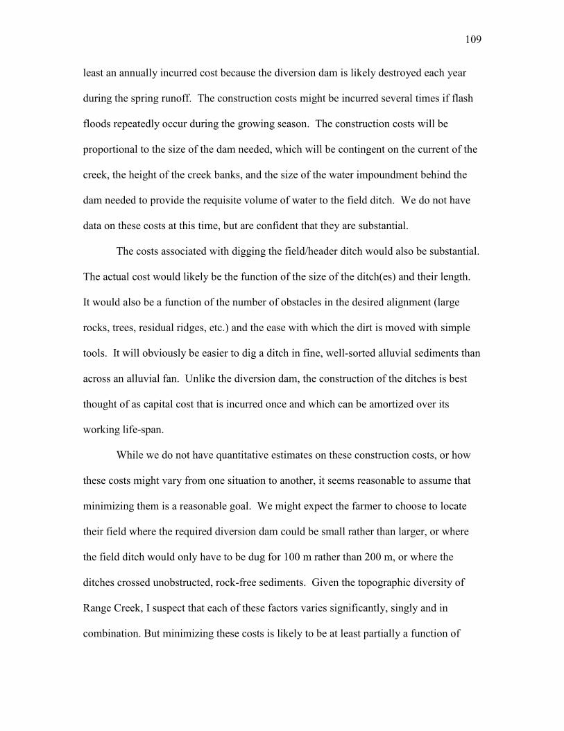
109
least an annually incurred cost because the diversion dam is likely destroyed each year
during the spring runoff. The construction costs might be incurred several times if flash
floods repeatedly occur during the growing season. The construction costs will be
proportional to the size of the dam needed, which will be contingent on the current of the
creek, the height of the creek banks, and the size of the water impoundment behind the
dam needed to provide the requisite volume of water to the field ditch. We do not have
data on these costs at this time, but are confident that they are substantial.
The costs associated with digging the field/header ditch would also be substantial.
The actual cost would likely be the function of the size of the ditch(es) and their length.
It would also be a function of the number of obstacles in the desired alignment (large
rocks, trees, residual ridges, etc.) and the ease with which the dirt is moved with simple
tools. It will obviously be easier to dig a ditch in fine, well-sorted alluvial sediments than
across an alluvial fan. Unlike the diversion dam, the construction of the ditches is best
thought of as capital cost that is incurred once and which can be amortized over its
working life-span.
While we do not have quantitative estimates on these construction costs, or how
these costs might vary from one situation to another, it seems reasonable to assume that
minimizing them is a reasonable goal. We might expect the farmer to choose to locate
their field where the required diversion dam could be small rather than larger, or where
the field ditch would only have to be dug for 100 m rather than 200 m, or where the
ditches crossed unobstructed, rock-free sediments. Given the topographic diversity of
Range Creek, I suspect that each of these factors varies significantly, singly and in
combination. But minimizing these costs is likely to be at least partially a function of

110
irrigating as large a field as possible with a single diversion dam and field canal. There
is an economic advantage when a large field or multiple fields can be irrigated from a
single diversion dam and single field canal. In sections of the canyon where the canyon
floor is broken into smaller parcels, either because of meanders in the creek channel or
the intrusion of ridges descending from the canyon walls, more diversion dams and
canals will be required than in areas with broad and unbroken expanses of arable land.
Another reason to suspect larger areas of arable land are more valuable is that
they may be better at accommodating growth. When farmers are investing heavily in their
fields, especially with irrigation, the ability to expand the size of their fields during good
times is likely to be a huge benefit. It would also better accommodate population growth
across generations. If we start with the simple proposition that there is some minimum
field size that is needed to support a family of maize farmers in this environment (Van
West 1994, 1996) then larger arable tracts, at least potentially, should allow surpluses
which could be used to improve the nutrition of the farmers, allow larger caches as
buffers in an uncertain environment, or be used in trade to improve the lot of the farmer
in many different ways. The alternative is to establish new fields, perhaps at some
distance from the original depending on land status and requiring the construction of an
additional irrigation system. There are a host of reasons why farmers should prefer to
have all their fields in one place (Hard and Merrill 1992:611).
Last, larger areas could potentially support greater numbers of families that
probably operated as independent or at least semi-independent consumptive units.
Having more neighbors likely increases the opportunity to cooperate in activities that
benefit the cooperators. Cooperating families could share the costs of the capital

111
investments associated with an irrigation system that served more than one family’s
fields. As discussed above, a single diversion could be used to feed a ditch that runs the
length of a large farmable area. Any family willing to share in the construction and
maintenance could benefit by reducing the cost per family. This would reduce the costs
associated with a single family having to build and maintain a simple irrigation system of
their own because even if the length of ditch required to irrigate a smaller field was
reduced, the costs associated with building and maintaining a diversion dam to water a
small field are the same as those for a larger field. Without cooperating neighbors to
share the costs, a single family irrigating a small field would pay all the costs for a
diversion and ditch. Cooperating neighbors would divide those costs for the same efforts.
Considering the influence of these factors on reducing irrigation costs, the size of
the arable tracts of land seemed a reasonable first approximation to have significant
influence on the value of the land and the settlement pattern of the Fremont farmers. The
first step in identifying contiguous tracts of arable land in Range Creek Canyon was to
identify those areas of the canyon floor that are relatively flat and composed of
sediments. I recognize that farming can occur in nonoptimal areas if farmers are willing
to invest in clearing rocks, perhaps terracing hillsides, constructing long field ditches for
surface irrigation systems, etc., but the evidence to date does not suggest that the Fremont
farmers utilized any of these expensive options to farm in the canyon. So I used
relatively simple criteria for identifying potentially farmable land: relatively flat areas on
the canyon floor, close to a source of irrigation water, and the presence of alluvial
sediments. The latter was employed to eliminate flat areas on the toes of ridgelines

112
extending into the canyon. The toes of these ridges have little or no sediment
accumulation and would be very poor candidates for farming.
Valley Floor and Slope
The simplest way to identify arable land is to limit farmable land on canyon floor
areas to at or below a specific slope. The Natural Resources Conservation Service of the
United States Department of Agriculture identifies the “gently sloping” class of slopes as
ranging between 1 and 8 percent (USDA NRCS 2010). Studies of ideal topographic
conditions for farming identify a slope between 0-15 percent as “gently sloping”
(Afyuni et al. 1993; Nurmiaty and Baja 2013; Venkateswarlu 2001). Gentle slopes
generate less surface erosion, have increased moisture holding potential, and require less
field preparation for surface irrigation (NEH 1991; USDA NRCS 2010). Based on the
change in slope gradient between the alluvial canyon floor and the base of the cliff walls
in Range Creek Canyon, I identified less than or equal to a 12 degree slope as a
reasonable limit. I also eliminated the side canyons from further consideration. There are
no perennial water sources other than a few seeps in the side canyons, they are prone to
limited but frequent flash floods, and their floors are characterized by much more poorly
sorted sediments than found in the main canyon.
Calculating Amount of Contiguous Arable Land
To empirically scale the amount of arable land along the canyon bottom, I used
the focal statistics tool in ArcGIS 10.1 which calculates a statistic of the values from a
neighborhood around an input cell location and generates a new raster layer from the

113
calculated values. I used this strategy because, in one sense, the entire floor of the canyon
within the study area is contiguous along its upstream/downstream axis. The strategy
described below basically scales changes in the amounts of arable land perpendicular to
the course of the creek. I created a raster layer that assigned a value of “1” to each 25 m²
grid cell with less than a 12 degree slope on the valley floor. Areas with a greater slope
than 12 degrees, or areas with less than 12 degree slope but located outside the valley
floor were assigned a value of “no data.” I ran the focal statistic calculation that searched
for continuous 25 m² blocks of land with less than a 12 degree slope within a specified
distance from each cell.
I used a circle for the shape of the search neighborhood around each cell and
varied the search radius used for several iterations of the analysis and compared each
output. I started with a large radius of 400 m which captures the entire canyon floor at its
widest stretch. I then incrementally decreased the radius until I reached 100 m. A 400 m
search radius was too coarse because it spanned the toes of ridgelines in the upper canyon
and artificially elevated the importance of the sinuous character of the canyon floor in
these reaches.
The results of using a 100 m radius were equally problematic; the entire canyon
floor was highlighted as one long contiguous locus. All the variability in the east-west
dimension of the canyon was lost. A 250 m search radius minimized both of these
problems by constraining the analysis to the valley floor and away from the ridgelines,
without losing the east-west dimension of variability (Figure 3-18). A 250 m radius
keeps the search neighborhood below the maximum distance east to west (~650 m) of the
area designated valley floor. The resulting calculation of amount of arable land became

114
one base layer for exploring the spatial distribution of other aspects of the environment
that constrain farming productivity in Range Creek Canyon. It also provides the basis for
an analysis of the location of residential alignments relative to the estimated amount of
farmable area.
Amount of Arable Land--Results
In Figure 3-18, grid cells that make up the largest contiguous amount of arable
land are shown in red and areas with the least contiguous arable land are shown in blue.
When using a 250 m radius, the largest amount of suitable neighboring land is 0.19 km²,
the smallest 25 m², or 0.000025 km². The size of similarly colored sections, and their
color, is a measure of the amount of arable land present.
Figure 3-18 shows several sections of canyon floor with the largest areas of
contiguous arable land denoted by orange to red highlighting. Section 1 is the southern-
most section and includes about 247 hectares of arable land. It has a single, centrally
located locus with values approaching 0.19 km². That locus includes about 42 ha with a
maximum width of 0.4 km and length of 2 km, measured along the creek.
Section 2 which is essentially one large reach of the canyon with values
approaching 0.19 km² (Figure 3-18). This section of canyon floor is the widest in Range
Creek, reaching a maximum width of 600 m and it is about 10 km in length. There are
306 ha of arable land in Section 2.
Section 3 is topographically quite distinct from Sections 1 and 2. This section of
Range Creek Canyon has a narrow canyon floor that weaves between the alternating toes
of ridges descending from the bordering highlands. Section 3 includes about 184 ha of

115
arable land with three distinct loci of concentrated arable land. Moving south to north,
locus 3A (Figure 3-18) includes an area of about 15 ha along 2 km of the creek with a
maximum width of .3 km. Locus 3B about 3 km long with a maximum width of .3 km.
Locus 3C includes about 22 ha and measures about .3 km by 1 km (Figure 3-19).
All things being equal, if contiguous arable land was the only factor controlling
“value” for farming, the red areas on the map would indicate the most valuable farming
areas in the canyon. Chapter 4 discusses the implications of this variable and other
variables affecting farming productivity in Range Creek Canyon and analyzes the
location of prehistoric residential rock alignment features relative to those locations
identified as potentially highly suitable for maize farming.
Soil Texture
Soil texture is one of four physical aspects of the environment affecting corn
production that arguably played an important role in the farming success of prehistoric
populations who lived in Range Creek Canyon. The spatial distribution of soil types has
likely remained relatively static in Range Creek Canyon with the same formation
processes at work and minimal variation in parent material throughout the canyon.
The soil texture is crucial to farming success because the water holding capacity,
the intake rate, and the drainage rate is largely a function of the texture of the soil
(Rhoads and Yonts 1991, NEH 1991). Soil texture is a classification of the relative
proportion of sands, silt, and clays which separate when dispersed in fluid. I used two
tests to capture the variability in soil texture in Range Creek Canyon. The first is a simple
soil texture test used to identify vertical changes in soil texture in the experimental farm

116
plots. The second identifies near-surface changes in soil texture and chemistry from north
to south along the canyon bottom.
Soil Texture in Farm Plots
To determine the textural characteristics in the vicinity of the farm and control
plots, a small exploratory pit was excavated to a depth of 70 cm (28 in) just outside of the
experimental plots. Soil samples were collected from the exposed profile in 10 cm (4 in)
increments (Figure 3-20). A simple soil texture test was conducted on each sample (Day
1965; Gee and Bauder 1986). The proportion of sand, silt, clays, and gravel was
measured and their relative percentages calculated. The type of soil was identified using
the standard soil texture triangular chart. Additional soil samples are available for future
analyses.
Soil Texture on Canyon Bottom
Soil samples were collected from the valley floor along the length of the Range
Creek Field Station. The canyon floor within the field station was divided longitudinally
into 15 sections. Three soil samples were collected in a generally systematic manner
across each section for a total of 45 samples. The samples within each section were taken
from the alluvium/sagebrush flats within 50 paces east or west of the creek. The samples
were collected by scraping back the surface material (approximately 4 cm [2 in]) and then
collecting two cups of soil from between approximately 4-20 cm (2-8 in) below ground
surface into a plastic bag. The precise locations were recorded with a GPS. Notes on
each sample included location description, setting, vegetation, and direction from the

117
creek. Several overview photographs were taken from each sample location. Every other
sample north to south between the gates of the field station, was selected for analysis.
Samples were sent to the Utah State University Analytical Laboratories (USUAL) for
chemical and texture testing. The soil properties of interest were selected following
Benson’s 2010 study of agricultural productivity in the Southwest and included texture,
pH, electrical conductivity, phosphorus, potassium, total nitrogen and total carbon. One
of the samples did not have enough material for complete analysis which resulted in 20
complete soil samples.
Soil Texture--Results
Results from the soil texture test show that the percentage of sands compared to
the percentage of silts was high at all depths in the soil profile. No clays were detected in
this test but plenty of soil is left for further testing using higher precision equipment. No
“hard pan” barriers were encountered between 0-70 cm 0-28 in) below ground surface
that might impede corn root depth. No gravels were encountered which might have
hindered root development or changed the water holding potential of the soil. The soil in
the profile was classified as loamy sand in all but two of the 10 cm (4 in) levels tested
(Table 3-4). Two of the layers barely crossed the threshold into the sand category.
An important attribute of soil texture is its ability to retain moisture. A number of
terms are used to measure this attribute. The water content of a soil when saturated and
allowed to drain is called the field capacity (Rhoads and Yonts 1991). The permanent
wilting point is the point at which a crop can no longer take water up from the soil and
cannot recover overnight from excessive drying during the day. Other authors tend to use

118
terms like storage capacity, holding capacity, and available water interchangeably to
discuss the range in amount of water available between the field capacity and the wilting
point (Rhoads and Yonts 1991). I will be discussing the field capacity, the maximum
amount of water available for each soil type, and the depletion by maize plants at varying
growth stages.
Field Capacity
Because of the larger grain size, sandy soils do not have a high field capacity
compared to smaller-grain sediments (Rhoads and Yonts 1991: Table 1:2). Sandy soils
generally drain more quickly and need to be irrigated more frequently than clay or loam
soils. The top 10 cm (4 in) of our soil profile is sand which might drain slightly faster
than the loamy sand below. For loamy sand, the field capacity is 1.1 inches/foot. Corn is
capable of using about 50 percent of the field capacity before suffering water stress
(Rhoads and Yonts 1991:1).
In the early stages of plant growth, less water is required than in later stages when
a mature plant with larger leaf area is pulling water from the soil profile (Rhoads and
Yonts 1991: Table 3:2). Once the maize plant has used 0.55 of the 1.1 inches per foot, the
soil moisture needs to be replenished or maize productivity will decrease (Rhoads and
Yonts 1991:2). Replenishing the available moisture is particularly important in the weeks
leading up to the reproductive stage and during the cob development stage that follows,
approximately 4 weeks centered around the time of silking and tasseling (Adams et al.
1999; Adams et al. 2006; Benson 2010a; Shaw and Newman 1990). Seventy-five percent
of the root system of a mature field corn or sweet corn is in the top 12 in of soil (Rhoads

119
and Yonts 1991, Figure 1:3) but the roots steadily increase in size and depth during and
after the reproductive phase until the corn cobs reach physiological maturity, and
subsequently use more and more water. Before this experiment, I didn’t know much
about the rooting depth of Tohono O’odham but between the readings from the soil
moisture sensors (discussed in Chapter 2) and the visual indicators of plant stress, it was
clear the plants were not getting enough water in the plots that were not irrigated
frequently.
Soil Properties from Canyon Floor
Data obtained from analysis of the 21 surface sediment samples from along the
canyon floor are reported in Table 3-5 (Sandy loam abbreviated as SL and Loamy Sand
abbreviated as LS). The number of the sample location corresponds to the numbered
sample areas shown on Figure 3-21. Of particular interest for this study are the results of
the soil texture analysis which show loam, loamy sand, and sandy loam present for most
of the sampled valley floor. Despite these samples coming from the upper 20 cm (8 in) of
the soil profile, it provides an estimate of what might be present at greater depths if the
same depositional processes have been relatively uniform for the past thousand years.
Analysis of samples from greater depths in the future will verify this assumption and
identify any variation from the loam to sand range of textures that dominate the soil
profile on the valley floor in Range Creek Canyon.
While the soils in the experimental plot were dominated by loamy sand with a
field capacity of 1.1 in/ft, the range of soil textures from north to south from the valley
floor samples demonstrate greater variation. Areas with soils dominated by loam have a

120
higher field capacity than sandy loam or sand. Loam, depending on the percentage of
very fine silts or sand, can range between 2 and 2.5 inches per foot in field capacity
(Rhoads and Yonts 1991). Those areas estimated to have a high percentage of loam are
indicated in black (Figure 3-21). The field capacity for sandy loam is 1.4 inches per foot.
These areas of the canyon floor are indicated in dark gray (Figure 3-21).
Sample 12a from the canyon-wide survey is spatially the closest to the location of
the 2014 experimental plots. Sample 12a is classified as loam, while the samples
adjacent to the experimental plots ranged from sand to loamy sand, suggesting that there
might be greater spatial variation than captured by our preliminary survey. This might
also be a function of utilizing different tests to determine soil texture (lab test vs. simple
field test). For now the best estimate for soil water field capacity in Range Creek Canyon
is a range from 1.1-2.5 in/ft. Using the surface samples to estimate the best areas for
moisture holding potential in the canyon, the loam areas, is a starting point that can be
refined as additional data become available.

121
Figure 3-1. Relief map of lower Range Creek Canyon showing the location of two automated weather stations and the 11 manual rain gauges. Note the location of the
experimental corn field near rain gauge 10.
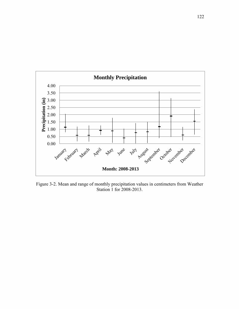
122
Figure 3-2. Mean and range of monthly precipitation values in centimeters from Weather Station 1 for 2008-2013.
0.00 0.50 1.00 1.50 2.00 2.50 3.00 3.50 4.00
Prec
ipita
tion
(in)
Month: 2008-2013
Monthly Precipitation
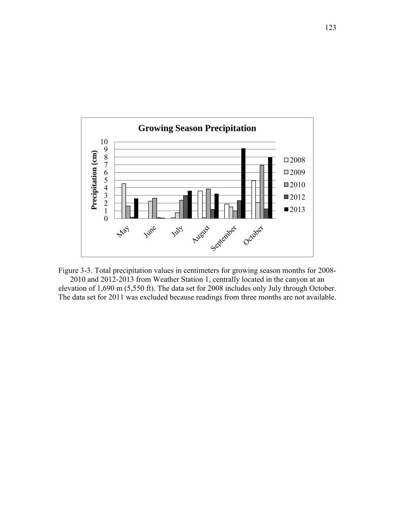
123
Figure 3-3. Total precipitation values in centimeters for growing season months for 2008-2010 and 2012-2013 from Weather Station 1, centrally located in the canyon at an
elevation of 1,690 m (5,550 ft). The data set for 2008 includes only July through October. The data set for 2011 was excluded because readings from three months are not available.
0 1 2 3 4 5 6 7 8 9
10
Prec
ipita
tion
(cm
)
Growing Season Precipitation
2008 2009 2010 2012 2013

124
Table 3-1
Total Precipitation from Rain Gauges
Rain gauge no. 2013 (May-December)
2014 (May-October)
total precip. (in/cm)
total precip. (in/cm)
RG-1 10.76/27.33 8.28/21.03
RG-2 8.47/21.51 7.26/18.44
RG-3 8.13/20.65 8.28/21.03
RG-4 7.84/19.91 8.14/20.68
RG-5 7.29/18.52 8.88/22.56
RG-6 7.11/18.06 5.69/14.45
RG-7 7.31/18.57 7.2/18.29
RG-8 7.62/19.35 7.3/18.54
RG-9 n/a 5.26/13.36
RG-10 7.01/17.81 5.65/14.36
RG-11 5.4/13.72 5.18/13.16
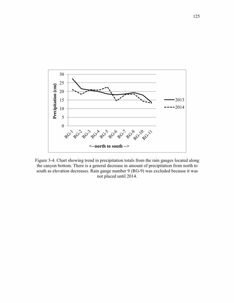
125
Figure 3-4. Chart showing trend in precipitation totals from the rain gauges located along the canyon bottom. There is a general decrease in amount of precipitation from north to south as elevation decreases. Rain gauge number 9 (RG-9) was excluded because it was
not placed until 2014.
0
5
10
15
20
25
30
Prec
ipita
tion
(cm
)
<--north to south -->
2013 2014

126
Figure 3-5. Contour map of the hydrologic basin draining into Range Creek Canyon, showing the average precipitation received annually over the last 30 years.

127
Figure 3-6. Contour map of the hydrologic basin draining into Range Creek Canyon, showing the average precipitation received from June through September over the last 30
years.
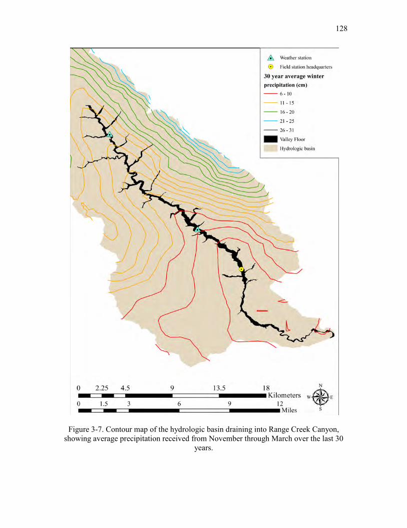
128
Figure 3-7. Contour map of the hydrologic basin draining into Range Creek Canyon, showing average precipitation received from November through March over the last 30
years.
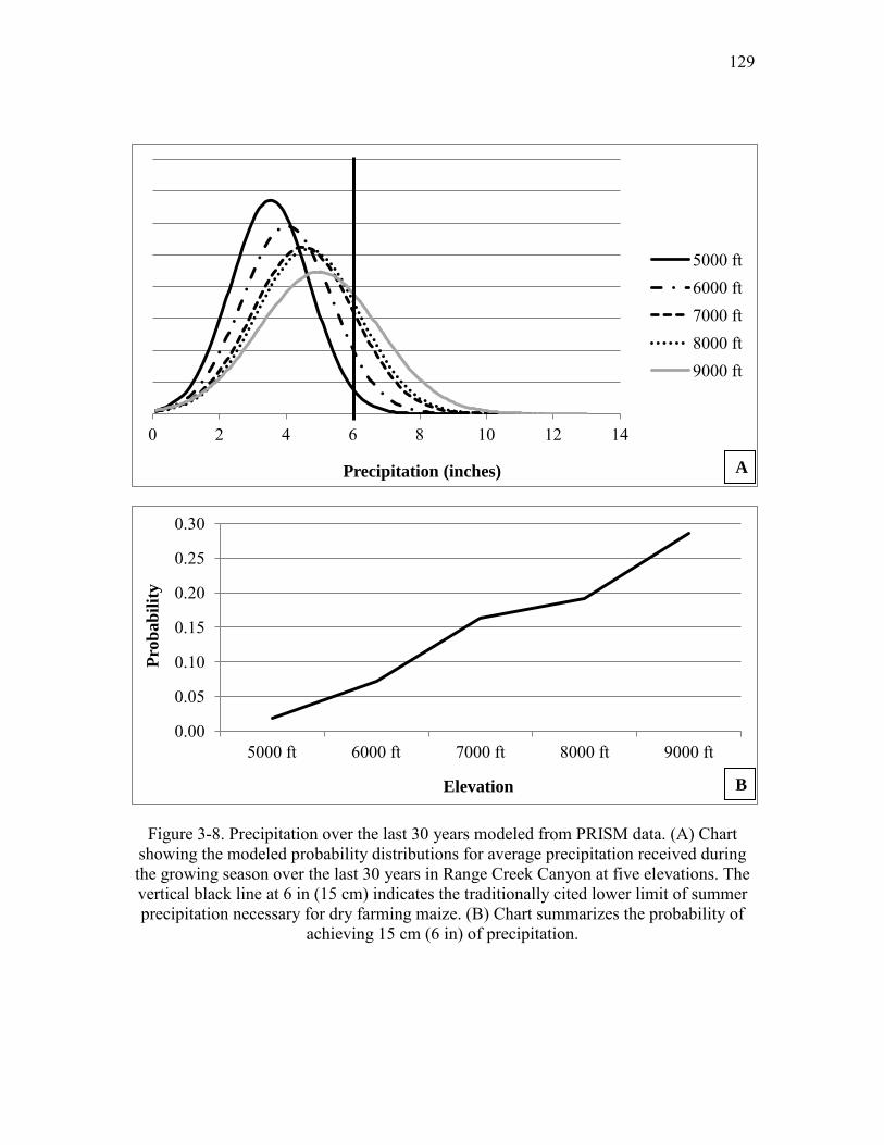
129
Figure 3-8. Precipitation over the last 30 years modeled from PRISM data. (A) Chart showing the modeled probability distributions for average precipitation received during the growing season over the last 30 years in Range Creek Canyon at five elevations. The vertical black line at 6 in (15 cm) indicates the traditionally cited lower limit of summer precipitation necessary for dry farming maize. (B) Chart summarizes the probability of
achieving 15 cm (6 in) of precipitation.
0 2 4 6 8 10 12 14
Precipitation (inches)
5000 ft 6000 ft 7000 ft 8000 ft 9000 ft
0.00
0.05
0.10
0.15
0.20
0.25
0.30
5000 ft 6000 ft 7000 ft 8000 ft 9000 ft
Prob
abili
ty
Elevation
A
B
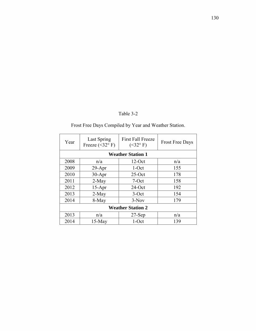
130
Table 3-2
Frost Free Days Compiled by Year and Weather Station.
Year Last Spring Freeze (<32° F)
First Fall Freeze (<32° F) Frost Free Days
Weather Station 1 2008 n/a 12-Oct n/a 2009 29-Apr 1-Oct 155 2010 30-Apr 25-Oct 178 2011 2-May 7-Oct 158 2012 15-Apr 24-Oct 192 2013 2-May 3-Oct 154 2014 8-May 3-Nov 179
Weather Station 2 2013 n/a 27-Sep n/a 2014 15-May 1-Oct 139

131
Table 3-3
Cumulative Growing Degree Day Requirements for Modern Maize Hybrid
Phase Development Stage CGDD
Vegetative
planted 0 two leaves fully emerged 200 four leaves fully emerged 345 six leaves fully emerged 475 eight leaves fully emerged (tassel beginning to develop) 610
ten leaves fully emerged 740
Reproductive
twelve leaves fully emerged (ear formation) 870 fourteen leaves fully emerged (silks develop on ears) 1000 sixteen leaves fully emerged (tip of tassel emerging) 1135 silks emerging, pollen shedding (plant at full height) 1400 kernels in blister stage 1660 kernels in dough stage 1925 kernels denting 2190
Maturation kernels dented 2450 physiological maturity 2700

132
Figure 3-9. Chart showing the CGDD for 2009-2014 from Weather Station 1 with a planting date of May 8th (the day after the latest spring freeze for all years).

133
Figure 3-10. Showing the difference in CGDD between Weather Station 1 (mean for years 2009-2014 last spring freeze May 8th) and Weather Station 2 (2014 full year with
last spring freeze May 16) with a difference in elevation of 370 m (1,210 ft).

134
Figure 3-11. Chart showing the estimated CGDD for increasing elevation and decreasing temperatures between Weather Station 1(mean for 2009-2014) and Weather Station 2
(2014 only). Note the first fall freeze at Weather Station 2 (2,060 m [6,760 ft] elevation) on October 01, 2014.

135
Figure 3-12. Chart showing the estimated CGDD for increasing elevation and decreasing temperatures between Weather Station 1 (mean for 2009-2014) and Weather Station 2 (2013 fall). Note the first fall freeze at Weather Station 2 (2,060 m [6,760 ft] elevation)
on September 27, 2013.

136
Figure 3-13. Map showing the 2,000 m (6,560 ft) elevation contour in Range Creek Canyon. Based on the CGDD required for the experimental maize to reach full maturity,
planting above 2,000 m (6,560 ft) would be risky in cool years.

137
Figure 3-14. Chart showing the modeled probability distributions for average FFD over the last 30 years in Range Creek Canyon at five elevations. (A) The vertical black line
indicates the 120 FFD. (B) Chart showing the modeled probability distributions for average CGDD over the last 30 years in Range Creek Canyon at five elevations. The
vertical black line indicates 2250 CGDD.
50 100 150 200 250
Frost Free days
5000 ft 6000 ft 7000 ft 8000 ft 9000 ft
500 1000 1500 2000 2500 3000 3500 4000
Cumulative Growing Degree Days
5000 ft 6000 ft 7000 ft 8000 ft 9000 ft
A
B

138
Figure 3-15. Chart showing the probability of achieving ≥ 120 frost free days (FFD) and ≥ 2250 CGDD in Range Creek Canyon at five elevations over the last 30 years (PRISM
dataset 1981-2010).
0.00
0.20
0.40
0.60
0.80
1.00
5000 ft 6000 ft 7000 ft 8000 ft 9000 ft
Prop
ortio
nal P
roba
bilit
y
Elevation
> 120 FFD > 2250 CGDD

139
Figure 3-16. Chart showing the proportional probability of achieving ≥ 1800 CGDD in Range Creek Canyon at five elevations (PRISM dataset 1981-2010).
0.00
0.10
0.20
0.30
0.40
0.50
0.60
0.70
0.80
0.90
1.00
5000 ft 6000 ft 7000 ft 8000 ft 9000 ft
Prop
ortio
nal P
roba
bilit
y
Elevation

140
Figure 3-17. Chart showing the probability of receiving ≥ 6 in (15 cm) of precipitation and ≥ 2250 CGDD at five elevations in Range Creek Canyon.
0.00
0.20
0.40
0.60
0.80
1.00
5000 ft 6000 ft 7000 ft 8000 ft 9000 ft
Prop
ortio
nal P
roba
bilit
y
Elevation
> 2250 CGDD
> 6" (15 cm) Precipitation

141
Figure 3-18. Map scaling the contiguous arable land available on the valley floor in Range Creek Canyon. Areas in red have the largest amount of contiguous arable land. Three sections of the topography and associated hotspots for farming are identified.

142
Figure 3-19. Map showing the valley floor in Range Creek Canyon split into three sections and the corresponding loci for contiguous arable land in each section.

143
Figure 3-20. Photograph showing soil profile sample for soil texture analysis, located outside Plot 2.
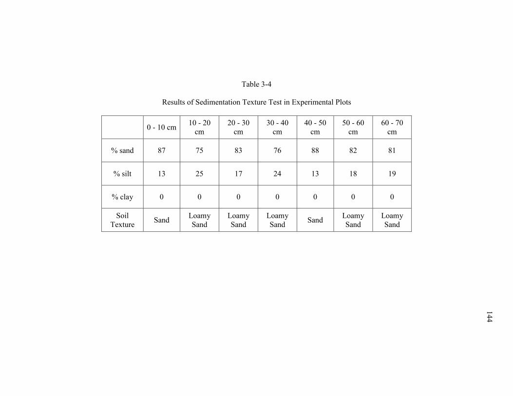
Table 3-4
Results of Sedimentation Texture Test in Experimental Plots
0 - 10 cm 10 - 20 cm
20 - 30 cm
30 - 40 cm
40 - 50 cm
50 - 60 cm
60 - 70 cm
% sand 87 75 83 76 88 82 81
% silt 13 25 17 24 13 18 19
% clay 0 0 0 0 0 0 0
Soil Texture Sand Loamy
Sand Loamy Sand
Loamy Sand Sand Loamy
Sand Loamy Sand
144

145
Figure 3-21. Map of lower Range Creek Canyon showing the location of 21 surface soil samples analyzed for texture and chemistry. Large circles indicate soil texture
determinations for the point sampled and an estimated soil texture for surrounding areas.

146
Table 3-5
Results of Canyon-wide Surface Soil Analysis
USU ID
Sample location Texture pH EC Phosphorus Potassium Total
Nitrogen Total
Carbon dS/m ----------mg/kg----------- -----------%--------
5676 03b Loam 7.4 0.90 30 387 0.32 3.44
5677 04a Loam 7.4 0.68 13.7 234 0.17 1.62
5678 04c Loam 7.3 0.89 19.2 391 0.29 3.20
5679 05b SL 7.6 0.81 14.5 206 0.14 1.78
5680 06a SL 7.5 0.82 10.8 245 0.15 1.73
5681 06c SL 7.5 0.71 14.6 311 0.22 2.40
5682 07b Loam 7.6 0.65 20.6 230 0.19 2.15
5683 08a SL 7.8 0.35 6.3 163 0.10 1.19
5684 08c Loam 7.5 0.77 7.3 362 0.15 2.92
5685 09b N/A 7.7 0.86 n/a n/a 0.15 2.10
5686 10a Loam 7.8 1.21 4.6 352 0.16 1.67
5687 10c Loam 7.5 0.67 15.0 246 0.16 2.69
5688 11b Loam 7.9 1.02 9.1 213 0.28 3.78
5689 12a Loam 7.8 1.02 28 705 0.23 3.26
5690 12c SL 8.1 1.60 25 475 0.10 2.42
5691 13b SL 7.8 0.52 8.1 319 0.08 1.13
5692 14a SL 8.1 0.51 5.2 352 0.50 1.53
5693 14c SL 8.2 0.45 5.7 133 0.05 1.49
5694 15b SL 7.9 0.41 8.1 221 0.06 1.02
5695 16a LS 8.2 0.52 8.9 211 0.06 1.28
5696 16c LS 8.1 0.67 6.8 182 0.06 1.20

CHAPTER 4
ARCHAEOLOGICAL IMPLICATIONS
Understanding modern environmental constraints on farming success by
experimentally growing maize is just a context for exploring the opportunities and
constraints faced by prehistoric farmers in Range Creek Canyon, to distinguish the likely
from the less likely suite of strategies related to farming, and develop those expectations
with respect to their archaeological consequences. As is true for any focused research, my
work ignores the many other equally interesting questions, many of which have emerged
out of the work reported here. For example, long term droughts will also adversely affect
the density and distribution of important wild foods, which would need to be considered
when droughts make farming less profitable, especially as it might relate to changing
demographic circumstances (Barlow 2002). Farming is but one dimension of life for the
Fremont who occupied Range Creek Canyon, and a much broader empirical database is
needed to predict how the Fremont would have negotiated the costs and benefits of living
in a highly variable environment and how their decisions are reflected archaeologically
(Metcalfe and Barlow 1992; Barlow and Metcalfe 1996; Beck 2008). The research
reported here is an important step towards achieving that goal.
In the preceding chapters, I explored the environmental constraints on farming
and the impacts of water availability on maize yields. In this chapter, I will explore the

148
implications of those findings for understanding the archaeological record and the
settlement patterns of the Fremont in Range Creek Canyon.
Settlement Pattern Studies
The most general definition of settlement patterns in archaeology is the way in
which people distribute themselves across a landscape (Trigger 1989). This may be
small-scale, site level analyses or broader, community-based or regional patterns (Willey
1953). Settlement patterns have been used as a source of information about many aspects
of human behavior including economic, social, and political organization (Willey 1953).
Archaeological settlement patterns are thought of in terms of a hierarchy of levels:
activity areas within structures, associated activity areas around structures, communities,
and the distribution of communities across landscapes. Each level has been shaped by
factors that differ in kind or degree from other levels. Individual structures reflect family
organization, settlements reflect community structure, and regional distributions reflect
the impact of economics, subsistence, trade, administration, and regional defense.
In the late 1930s, research reported by Julian Steward on aboriginal social
organizations influenced the rise of regional-scale investigations to infer sociological
processes from changes in settlement patterning (Parsons 1972). Early examples of this
work include the Mississippi Valley Survey (Phillip et al. 1951) and Viru Valley project
(Willey 1953). By the 1950s, efforts were made to predict the archaeological
manifestations of different community patterns (Willey 1956); and by the late 1950s, the
importance of ethnographic analogy in settlement pattern studies was clearly evident
(Parsons 1972). In many ways, David H. Thomas’s long and productive exploration of

149
settlement patterns in a variety of contexts captures the last 40 years of development in
this dimension of anthropological archaeology.
Thomas’s early work in the Reese River Valley of central Nevada is an excellent
example of combining ethnographic analogy and quantitative techniques. Thomas (1973)
developed a quantitative model based on Steward’s (1938) ethnographic description of
Shoshone life ways that was incorporated into a computer program, BASIN I, which
simulated 1000 years of the described activities. Temporal differences were built into the
program based on annual variation in antelope populations, and pinion and wild seed
harvests. Thomas then conducted a stratified random survey of all the major biotic
communities in a section of the Reese River Valley to test his predictions about the
character of the frequency, types and distribution of artifacts within and between these
ecological strata. Over 75% of his predictions were met, and many of the rejected
predictions likely failed as the consequence of factors not included in his model (i.e.,
location of lithic source material and the influence of curated technologies). Despite its
remarkable success, the results of the Reese River Ecological Project are strongly limited
in time and space. Based on the projectile points recovered, the time depth of the
investigation is limited to the past 4,500 years. This period broadly encompasses the Late
Holocene, a time span where the climate and environment were similar to those of today.
There are also important features of the natural environment of Reese River Valley that
structured Shoshone life ways in significant ways that are not found in many other central
Great Basin valleys, not the least of which is the presence of a perennial stream. It is
unclear just how far back in time, or how far away from Reese River Valley, Thomas’s
reconstruction can be legitimately exported.
150
Upon completion of the Reese River Ecological Project, Thomas began a
settlement pattern study of another central Nevada valley, Monitor Valley (Thomas
1983). Unlike Reese River, Monitor Valley lacked a perennial stream, and it lacked a
detailed ethnographic description of Shoshonean adaptations to its natural environment,
but it did have a rockshelter with very deep and stratified deposits, Gatecliff Rockshelter.
Thomas consequently employed Binford’s (1980) middle-range theory of the “collector-
forager” spectrum as the baseline for investigation. Using a sophisticated survey
methodology, Thomas completed fieldwork with the goal of identifying sites associated
with either collecting or foraging strategies. He demonstrated that ethnographic Great
Basin bands crossed the entire spectrum from full-time foragers, to seasonally mixed
foragers and collectors, to full-time collectors within a radius less than 100 km (Bettinger
1991; Thomas 1983 and 1985; Zeanah 2002). Thomas was concerned not with
ethnographic analogy, “but with defining the underlying strategies for exploiting the
individual resources” (Thomas 1983: 40). While Thomas’s study identifies a remarkably
broad range of variability in bands that presumably shared the same culture, technology,
and language, the forager-collector model fails to explain that variability (Thomas 1983
and 2008; Zeanah 2002).
Behavioral Ecology Approaches to Settlement Pattern Study
In 2008, Thomas published a series of monographs chronicling his archaeological
investigations on St. Catherine’s Island on the coastline of the state of Georgia (Thomas
2008). In the St. Catherine’s Island research, Thomas explicitly employed the perspective
of behavioral ecology, which studies human behavior using the principles of natural
151
selection to understand adaptive strategies within its ecological context. Thomas
specifically used optimal foraging theory, aided by data gathered experimentally, to
interpret the results of the surveys and excavations. Thomas is explicit about shifting to
this perspective because of the ambiguous results from using “mid-range theory” in
Monitor Valley (Thomas 2008:4).
Foraging models. An approach grounded in behavioral ecology and more
specifically optimal foraging theory, allowed Thomas to simplify his assumptions and
constraints to make testable hypotheses about forager decisions within a particular
environmental landscape (Thomas 2008 and 2012). Optimal foraging theory focuses on
subsistence-related patterns expected if foragers make decisions that maximize their net
rate of energy capture while foraging (Winterhalder 1981). Foragers who act optimally,
efficient relative to time or energy costs in subsistence acquisition, are expected to have a
higher inclusive fitness than those that do not, and hence be favored by natural selection
(Winterhaulder 1981). The model simplifies the number of parameters acting on the
individual forager, allowing a basic set of predictions about various aspects of their
subsistence strategies under specified environmental conditions.
Thomas spent a great deal of time reconstructing the environmental landscape and
change through time at St. Catherine’s Island. The research team spent two years
conducting experiments designed to gather data on foraging returns in the modern
environmental context and then used that data to interpret their archaeological research
(Thomas 2008). Thomas is remarkably successful in reconstructing aboriginal foraging
on St. Catherine’s Island by employing the insights of foraging theory and incorporating
variability in patch type, season, technology, and group composition (Thomas 2008).

152
This is highlighted in his consideration of how the sexual division of labor affects the
return rates for certain resources, particularly the scheduling of oyster and clam
harvesting, and how the goals of men and women may be different and even conflicting
(Thomas 2008:69).
Another successful example of utilizing behavioral ecology in the study of
prehistoric settlement patterns, and one much closer to home, is the work of David
Zeanah’s analysis of prehistoric settlement patterns in the Carson Sink of Nevada
(Zeanah 1996; 2004). Zeanah looked at residential site location in terms of the trade-offs
faced by men and women and their sometimes conflicting subsistence goals. The
reproductive success of women, in general, is constrained by access to resources suitable
for feeding offspring on a daily basis, which often limits their mobility. Men, on the other
hand, often target prey that is encountered less predictably but when acquired it provides
a public good, increasing reproductive success by attracting mates and building alliances
(Bird and O’Connell 2006; Zeanah 2004). These contrasting goals can directly influence
settlement decisions. Utilizing modern range data, estimates of the costs and benefits of
exploiting the available wild resources, and a clear distinction between the foraging goals
of males and females, Zeanah was able to accurately predict the locations of certain site
types and aspects of their assemblage composition. Zeanah found that proximity to
women’s target resources proved to be the optimal location for residential sites most of
the time. This prediction was met in the distribution of late prehistoric residential bases
being located close to women’s resources and the location of logistical field camps in
close proximity to men’s target resources (Zeanah 2004).

153
Ideal free distribution models. Several recent studies have explained
archaeological patterns in settlement and colonization using predictions from the ideal
free distribution (IFD) model (Allen and O’Connell 2008; Codding and Jones 2013;
Kennett 2005; Kennett et al. 2006; O’Connell and Allen 2012; Winterhaulder et al.
2010). The ideal free distribution model was developed by Fretwell (1972) to explain the
distributions of birds migrating into new habitats. It addresses the question of where an
individual should chose to settle when he or she has the option of settling in two or more
habitats that differ in profitability (i.e., available food resources, access to suitable shelter
or available mates, etc.) at some finite point in time. It is “ideal” in the sense that all the
actors have perfect information and there is no cost associated with moving from one
habitat to another.
The model is based on the observation that as habitats are settled and exploited,
the resources in those habitats are depleted at a rate proportional to size of the population
exploiting them: large populations will deplete resources more quickly than small
populations. From the perspective of the individual deciding where to settle, the goal is
to maximize her rate of return, which is a function of both the habitat quality and the
number of competitors. When in equilibrium, the ideal free distribution states that
competitors should distribute themselves between habitats such that each individual has
the same rate of return. Habitats that are twice as good as poor habitats should support
populations twice the size as those in poor habitats.
One should expect the first inhabitants to choose the best habitat but, over time,
with the depletion of resources and increased competition for existing resources, the
profitability of the best habitat will decline to that of the second best. At that point, we

154
should expect further individuals to begin to settle in what was originally the second-best
habitat. The most suitable habitats will always have the highest population densities, the
least suitable habitats the lowest (Allen and O’Connell 2008; Codding and Jones 2013;
Winterhaulder et al. 2010).
In many ecological circumstances, the advent of agriculture will result in the
decrease in the mobility and increase in territoriality. Under these circumstances, the
ideal despotic distribution (IDD) is the more appropriate model. In this model,
movement between “habitats” is not free and the selection of habitats is constrained by
exclusionary tactics and intergroup competition over predictable resources (Dyson-
Hudson and Smith 1978; Fretwell 1972). Farm fields, especially those that have been
improved through capital investments, become spatially conscribed and more predictable
resources (Codding and Jones 2013). For example, when farmers invest in building
irrigation ditches, diversion dams, field leveling, etc., activities that improve the
productivity of that field, then defending fields becomes an increasingly important
consideration. The importance of these factors should be evident in the prehistoric
settlement pattern in Range Creek Canyon.
Settlement Patterns in Range Creek Canyon
The perspective of behavioral ecology provides guidelines for understanding how
Range Creek might have been settled initially and then how increasing populations,
competition for suitable farm land, and access to irrigation water might have shaped the
pattern in site distributions seen archaeologically. Using environmental constraints on
farming success (amount of arable land, water availability, and growing season) and the

155
results of the maize farming experiment, I will compare the location of archaeological
sites identified to be “residential” to locations identified as most suitable for farming. I
will discuss how variability in temperature, water availability (precipitation and
irrigation), amount of arable land, and population density during the Fremont occupation
might have shaped their pattern of settlement.
Modeling Suitability
Benson and colleagues’ recent publications on prehistoric maize farming in the
American Southwest use models that reconstruct a number of environmental variables in
the past to understand climatic impacts on maize productivity and the expected
behavioral responses (Benson et al. 2013; Benson 2010a, 2010b; Benson et al. 2007:
Benson and Berry 2009). The most recent publication, Benson et al. 2013, guided our
farming research in Range Creek Canyon. In it they developed a relatively simple model
to estimate maize farming productivity in southwestern Colorado, specifically the region
around Mesa Verde. Using data from nearby weather stations, they created an elevation
dependent precipitation function to calculate the amount of annually available
precipitation at any elevation in the study area (Benson et al. 2013). These modern
constraints were then sequenced to the past using tree-ring sequences from Douglas-fir to
reconstruct the precipitation record for Mesa Verde between AD 600 and 1300.
Based on these estimates, Benson and his colleagues examined when dry farming
was possible during this time, using the 30 cm (12 in) and 50 cm (20 in) thresholds
discussed previously. They were not able to estimate the amount of summer versus
winter precipitation, nor variance in annual temperatures. Benson et al. 2013 suggested

156
an elevation of 2,380 m (7,800 ft) is the maximum elevation where farming would have
been possible in the project area. They cite Petersen’s 1988 study of the changing tree
line over the past150 years in the La Plata Mountains that suggests the growing season
above 2,200 m (7,200 ft) elevation is generally too short under modern temperature
conditions. During some periods in the past warmer temperatures would be expected but
the warmer temperatures that would have made farming possible above 2,200 m (7,200
ft) are accompanied by drought conditions (Benson et al. 2013: 2877). They were able to
estimate the 30 and 50 cm (12 and 20 in) precipitation contours over the study area
divided roughly into two zones: the Great Sage Plain (1500-2100 m) and the modern
farming belt (2010-2380 m elevation). The Great Sage Plain is considered highly
productive farming area for the Anasazi in southwestern Colorado (Benson et al. 2013:
2876) with a more reliable length of growing season.
This study found that, in the Great Sage Plain, during 89% of the years between
A.D. 600 and A.D. 1200 some maize could have been grown because they would have
received at least 30 cm (12 in) of precipitation: the lower precipitation limit, assuming
some significant proportion of this rain fell during the growing season. During years
where the estimate is for 50 cm (20 in) or more annual precipitation (which should
produce a good harvest with some assumption of the seasonality of that rainfall), they
found that the Great Sage Plain only reached this threshold 33% of the time during the
period of interest but, in 23% of that time the 50 cm (20 in) contour lay above the
elevation limit for length of growing season (Benson et al. 2013:2879). They concluded
that given the unpredictable nature of the annual precipitation in the study area, “Native
Americans would have had to generally farm at upper elevations where agriculture was

157
mostly limited by length and intensity of the summer growing season and (or) they would
have had to scatter their fields over a range in elevations in response to the variability in
inter-annual precipitation” (Benson et al. 2013:2879).
I evaluate the suitability for farming in Range Creek Canyon, a much smaller
study area, using spatial variation in precipitation, growing season, and arable land in
much the same way. Because of the presence of Range Creek, the water source, I also
demonstrate how that changes the options for farmers and consequently the optimal field
locations.
Modern Climate Suitability for Farming In Chapter 3, I used temperature (CGDD), precipitation, contiguous arable land
size, and soil texture to discuss the limits on suitable farm areas in Range Creek Canyon
under current climate conditions. While soil texture is a very important constraint on the
suitability of different locations in the canyon for farming, I only have cursory data
measuring spatial variability in soil characteristics at this time (see Chapter 3). I will
therefore not include soils characteristics in the analysis below.
The results of my own experimental maize crops are used as the basis for
evaluating the productivity of farming along the length of the floor of the canyon, with
particular attention to the influence of available water (see Chapter 2). I found that
variability in temperature and precipitation is high from year to year over the recent
record but it has remained relatively dry (in terms of maize farming) even at higher
elevations. Temperature and precipitation fluctuate greatly between seasons and years,
but based on the pattern in CGDD and mean annual precipitation values, an estimate of

158
the most suitable areas for farming under current weather conditions can be identified.
The most reliable areas for length of growing season and the necessary CGDD will be
below 2,000 m (6,500 ft) in elevation (Figure 4-1). At 1,520 m (5,000 ft) and 1,800 m
(6,000 ft) in elevation, the warm temperatures necessary for maize farming have been
available between 97-100% of the time over the last 30 years. At 2100 m (7000 ft), the
probability of achieving the required ≥ 2250 CGDD is 62% and decreases with elevation
until reaching zero at and above 2,400 m (8,000 ft).
Given the probability of receiving sufficient precipitation for maize farming
during the growing season over the last 30 years, no areas on the valley floor in Range
Creek Canyon would have been suitable for dry farming (Figure 4-1). Below 2,100 m
(7,000 ft), which I consider the upper elevation limit based on historic CGDD
calculations, precipitation has met the lower limits for dry farming (≥ 6 in/15 cm) only
between 2-16% of the time, depending on elevation. Even at elevations above 7,000 ft,
the probability of receiving ≥ 6 in (15 cm) of precipitation during the growing season has
been between 16-29%.
Figure 4-1 illustrates the changes in precipitation and cumulative growing degree
days for Range Creek Canyon. Under modern conditions, it is impossible to move high
enough in elevation to predictably obtain the growing season moisture need to farm corn.
The decrease in temperature limits corn farming today to the section of the canyon below
7,000 ft. While the climate in this canyon has undoubtedly changed fairly dramatically
over the past 2,000 years, today it is impossible to be a successful farmer without
irrigation.

159
Past Climate Suitability for Farming
It is clear that under current climatic conditions, the past 30 years in Range Creek
Canyon have been warm and dry. Arguments have been made that the climate during the
Fremont period was much more suitable for dry farming, possibly at times being both
warmer and wetter. Here I review the relevant research.
Dendroclimatology offers the most temporally precise reconstructions of past
climate in the American Southwest. And fortunately for us, Knight et al. (2010) report the
most comprehensive reconstruction of precipitation for the Tavaputs Plateau spanning
323 BC to AD 2005 based on tree-ring samples recovered just north of Range Creek
Canyon. This reconstruction uses a new tree-ring sequence constructed from Douglas fir
collected in Nine Mile Canyon at elevations ranging from 2,130 m to 2,225 m (6,990-
7,300 ft) in elevation which the authors called the Harmon Canyon chronology (Knight et
al. 2010). Nine Mile Canyon is the major drainage immediately north of Range Creek and
its archaeological record, also primarily related to the Fremont, shares many similarities
to the archaeology in Range Creek (Spangler 2000 and 2013).
Knight et al. (2010) identify periods of extreme wet or dry visible in the
reconstruction at several scales: annual, decadal, and centennial. This study could not
differentiate between precipitation falling in the summer versus the winter, although they
do demonstrate that ring-width is most sensitive to the annual precipitation from the
previous July to the current June (Knight et al. 2010:110). In their analysis of decadal
variability in precipitation, they rank wet and dry periods by magnitude, duration, and
intensity. Magnitude is defined as the maximum or minimum smoothed precipitation
value, and intensity is “defined as the percentage of years exceeding the extreme dry/wet

160
threshold in the episode” (Knight et al. 2010:5) which is the top or bottom 10% (z >1.25
on a standardized distribution) of their sample. Comparison with other tree-ring
sequences from four other locations in the west provided the context for assessing the
spatial scale of these prehistoric droughts evident in the Harmon Canyon chronology.
The period of interest for understanding farming in Range Creek Canyon is
between AD 900 and 1200. In the centennial-level analysis, the authors find that the
series between AD 500 and 1100 oscillates at a 70 to 150 year frequency with long-term
departures from mean conditions occurring during dry phases from early AD 1100s to
1300s (Knight et al. 2010:6). On the decadal scale, there are numerous episodes of dry
and wet departures from the mean, with variability in magnitude, duration, and intensity
(Figure 4-2). The frequency and magnitude of extreme dry and wet decadal oscillations
are relatively complacent between AD 731 and AD 1276 relative to the periods
proceeding and following this time span (Knight et al. 2010:6). Analysis of the data at an
annual scale finds similar episodes of stability with the frequency of both wet and dry
single year extremes decreasing between AD 820 and AD 1220 (Knight et al. 2010: 7).
While this pattern of general stability between the target years of A.D. 900 – 1200
might have favored farming during this period, the average annual precipitation was only
a bit wetter than it is today, which is too dry for dry farming. The mean annual
precipitation reported for the entire 2,300-year period is 37.6 cm for elevations ranging
from 2,130-2,225 m (6,990-7,300 ft). These elevations are currently higher than the
modern limits for reliably reaching the requisite cumulative growing degree days for
maize.

161
As discussed earlier, annual precipitation is a coarse measure of the rainfall useful
for farming. For dry farming, the most important variable is growing season
precipitation. If significant seasonal shifts in the annual precipitation were present
prehistorically, then the problem of receiving sufficient moisture for dry farming may be
more or less severe. From this perspective, it is important to examine the data more
closely during the 300-year period representing the height of the Fremont occupation.
We know that there is a lot of yearly variability around that mean even during a
generally dry or wet period. The severity of a drought that affects the amount of summer
precipitation could have devastating effects on maize yields, even in a single year. The
duration and magnitude of the drought might also affect the winter precipitation and
therefore the amount of irrigation water available from melting snow pack. Unfortunately
we do not know from this study how much of the precipitation was falling in the summer
versus winter nor do we have a reconstruction of temperatures. Extended periods of
drought that affect both summer and winter precipitation over a long period of time, no
matter how stable in terms of extremes, would force farmers to either abandon farming or
abandon the area.
Dry Periods
Knight et al. report some decadal trends that would have influenced farming
success, settlement patterns, and potential benefits of investment in irrigation. Figure 4-2
shows four major dry periods, as defined above, between A.D. 900 and A.D. 1200, and
two significant wet periods.

162
The first major dry period lasted 29 years, between AD 932 and A.D. 960, and
had a maximum deviation of 26.3 cm below the mean and a mean annual deviation of
12.0 cm (Knight et al. 2010:Table 2). They report that 10% of this 29-year period
exceeded their drought threshold. The second period of dry conditions occurred between
A.D. 970 and A.D. 1010. This period had a maximum deviation from the mean of 34.6
cm and a mean annual deviation of 16.2 cm. Seventeen percent of this 41-year period was
considered extremely dry. This drought was longer and more severe than the one that
ended in A.D. 960.
From A.D. 1033 to A.D. 1052 is the third major dry period. The maximum
deviation from the mean was 25.8 cm and it exhibits a mean annual deviation of 17.7 cm.
One quarter of this 20 year period below the drought threshold. Last, beginning in A.D.
1128 and continuing through A.D. 1161 was the fourth major dry period. During this
time, it attained a maximum deviation from the mean of 28.3 cm and a mean annual
deviation of 18.8 cm. The authors estimate that 21% of this 34-year long period was
below the threshold for a drought.
Taken together, during the period from A.D. 900 to A.D. 1200, the four major dry
periods include 124 years or slightly more than 40% of this 300-year period. If we limit
our attention to actual drought years, approximately 22 years fall into this category. Of
these dry periods, the lowest annual precipitation was approximately 3 cm. During the
A.D. 1128 – 1161 dry period, the average annual rainfall was about one-half of that for
the entire chronology, about 19 cm annually.

163
Wet Periods
Two significantly wet periods are evident in the Harmon Canyon chronology
between A.D. 900 and A.D. 1200. The first lasted from A.D. 1011 to A.D. 1032, with a
maximum deviation above the mean of 28.8 cm and a mean annual deviation of 19.6 cm
(Knight et al. 2010:Table 2). Twenty-seven percent of this 22-year period was extremely
wet, above what the authors refer to as the pluvial threshold. This is an annual
precipitation increase of about 50%. The second wet period lasted 16 years between A.D.
1073 and AD 1088. It had a maximum deviation above the mean of 31.5 and a mean
annual deviation of 29.8. This wet period was above the pluvial threshold 63% of the
time and represents an 80% increase above the overall mean.
Taken together, these two wet periods include 38 years out of the 300 years of
interest, or about 13% of that span. The second wet period received considerably more
moisture than the first. Maximum annual precipitation during this period was about 69
cm, receiving on average about 67 cm. During the first wet period, average annual
precipitation was about 57 cm. If significant proportions of this precipitation occurred
during the growing season, dry farming might well have been a successful strategy during
these wet periods.
Implications for Dry Farming
Knight et al. (2010) calculated a mean annual rainfall of 37.6 cm, roughly the
same as the modern weather in Range Creek Canyon over the last 30 years from trees
growing at elevations ranging from 2,130 m to 2,225 m (6,990-7,300 ft). If we ignore the
wet and dry periods discussed above, about 138 years had an annual precipitation during

164
the Fremont occupation roughly similar to the modern climate record. Dry farming
might have been possible if the majority of that precipitation occurred during the growing
season. It doesn’t today. As I summarized in Chapter 3, the average annual rainfall at
7,000 ft (2,100 m) is 39 cm (15.4 in) with an average11.4 cm (4.5 in) falling during the
growing season. If that seasonal distribution holds for the past, and we do not have any
information relevant to deciding whether it does or does not, then dry farming may have
been a best marginally successful during some of these years, impossible during most of
them.
This conclusion also applies to the 124 years within the four major dry periods.
With an average annual precipitation of 26 cm (A.D. 932 – 960), 22 cm (A.D. 970 –
1010), 20 cm (A.D. 1033 - 1052), and 19 cm (A.D. 1128 – 1161). Even if the entire
amount of precipitation fell during the growing season, the probability of bringing a corn
crop to maturation depending on that precipitation would have been approaching zero.
Dry farming may have been successful during the 38 years that were identified by
Knight et al. (2010) as being wetter than average. During these two periods, average
annual precipitation would have been about 58 cm (A.D. 1011 – 1032) and 68 cm (A.D.
1073 – 1088). These represent nearly 50% and over 80% increases in precipitation,
respectively. During each of these periods, especially the more recent one, dry farming
may well have been a relatively successful endeavor, especially at higher elevations.
When employing averages there is always the danger of forgetting that they are
simply a measure of central tendency. For normally distributed functions, half the
distribution is below the average, half above. For example, the modern mean summer
precipitation was 3.53 in (9 cm) over the last 30 years at 1,520 m (5,000 ft) in Range

165
Creek Canyon. If we use the often cited threshold of ≥ 6 in as the amount of rainfall
required during the growing season to be minimally successful at dry farming, then
prehistoric precipitations rates would have to be about 70% higher during this season
than they are today. But because we are dealing with means, even with the 70% increase,
sufficient rainfall would only occur about half the time (Figure 4-3).
Based on the above, the simple conclusion is that unless the precipitation
reconstructions for the past 2000 years seriously underestimate annual precipitation or the
seasonal distribution of precipitation was significantly different from what we see today,
dry farming would not have been a viable strategy for an estimated 262 of the 300 years
of interest. During the remaining 38 years, which are reconstructed as wetter than
average, dry farming may have been a viable strategy during some, but probably not all
of the wet years. Even during these wetter periods, during some years the growing
season rainfall would have failed to reach the minimum needed. Taken together, these
data support the conclusion that the Fremont in Range Creek practiced one or more forms
of irrigation. If they did not, then they were not farming in the canyon, which directly
contradicts the archaeological evidence.
It must be remembered that much of the data presented in the preceding sections
are statistical estimates, and in some cases, statistical estimates of data from statistical
estimates. We really do not know how these uncertainties might combine to influence
the accuracy of the reconstructions present above. But fortunately, the results are not on
the cusp, where a small change would dramatically alter the reconstruction. Range Creek
Canyon was a hub of activity between around A.D. 900 and A.D. 1200; the Fremont who
lived there farmed at least some of that time and during this span, it was still largely a

166
semi-arid environment. Range Creek, the principal water source in the canyon, was a
small flowing creek during much of this time. Farming in this canyon would have been
difficult no matter how you look at it. If there were times when it was so dry that the
creek dried up during the growing season, then the Fremont would have had to rely on
hunting and gathering wild resources, or moving somewhere else, but when water was
available, then they should have practiced irrigation.
This conclusion is given further support by the results of the farming experiments
reported in Chapter 2 that demonstrate that providing additional moisture to maize results
in a larger harvest. It is not just a question of whether the Fremont had to irrigate their
fields in Range Creek Canyon, but rather whether the benefits of irrigating were larger
than the costs. It is interesting to explore a couple of scenarios. A Fremont family moves
into Range Creek during a dry period or period of average precipitation. Based on the
available evidence, either they irrigate their crops or they survive by hunting and
gathering. Assuming the former, even during wetter years, when crops might have
reached maturity from rainfall alone, irrigating those same crops would have produced a
larger harvest. That is, even in wetter periods, the family would have benefitted by
irrigation due to larger harvests. Given that we suspect, but have not yet demonstrated,
that the greatest costs associated with irrigating relate to the capital costs associated with
constructing the ditches and dams associated with surface irrigation, deriving a benefit
even during wetter years provides an extended period of benefits against which to
amortizing those costs.
The alternative is that the Fremont family settles into Range Creek Canyon during
one of the wetter periods. Under these circumstances, depending on the costs of

167
constructing an irrigation system, they might postpone that construction. I suspect it is
far more likely that they would have been fully aware of the annual variance in summer
precipitation and more or less immediately began to clear a field and construct an
irrigation system. Even if an irrigation system was not constructed during the first year
or two, they would have staked a claim to a portion of the canyon bottom suitably
situated for irrigation. Either scenario leads to the same expectations concerning the
pattern of settlement in the canyon.
Archaeological Expectations for Settlement
Based on radiocarbon dates analyzed from prehistoric cultural contexts in Range
Creek Canyon, the peak of the Fremont occupation occurred around AD 1050
(Boomgarden et al. 2014). I have demonstrated that, based on the modern climate
records, the relationship between elevation and annual precipitation is positive, but the
slope of that relationship is shallow. Moving up in elevation, within the confines of the
canyon, never results in achieving sufficient growing season rainfall to reliably dry farm.
The relationship between elevation and frost free days and cumulative growing degree
days is equally strong, but in the opposite direction (Figure 3-15). Moving up in
elevation to gain the additional precipitation quickly runs into the countering force of
insufficient heat to bring a crop to maturity.
As I demonstrated in Chapter 3, the modern climate of Range Creek Canyon
ensures that there is effectively a zero percent chance of not reaching a 2250 cumulative
growing degree days at 5,000 ft (1,500 m) in elevation, only a 3% chance of not attaining
enough heat at 6,000 ft (1,800 m), but a 40% of failing at 7,000 ft (2,100 m). I have no
168
way of evaluating how the difference between zero percent and 3% is likely to have
played out in behavioral terms, but I am confident that establishing farm fields at 7,000 ft
(2,100 m) would rank well below planting fields at 6,000 ft (1,800 m) due to the
temperature differential. This is not to argue that people never farmed at or above 7,000
ft; the point is that farming at that elevation would only be expected if they did not have
the option of farming at lower elevations. For the purposes of my research, I model the
farming potential of the canyon bottom below 7,000 ft (2,100 m) as equal with respect to
temperature.
Given these data, the potential influence of settling higher in the canyon to take
advantage of greater annual rainfall in a quest to dry farm can be safely set aside. There
may have been other reasons for settling higher in the canyon, such as competition for the
water from the creek, but those are not considered here (but see Chapter 5). Although the
data are limited, there is not any reason to suspect that variation in soil texture along the
length of the canyon had much significance in the choice of where to farm on the canyon
floor. Within the set of constraints I am examining here, that leaves variation in the size
of contiguous arable land as an important factor in determining field and residential site
locations.
Open Residential Sites
To understand how prehistoric people chose to locate themselves with respect to
arable land and surface water, I examined the distribution of archaeological sites likely to
represent open residential locations. Open residential sites are defined as consisting of
one or more unsheltered surface rock alignments (Figure 4-4). Within the northern and

169
southern boundaries of the field station, these sites also had to include one or more of the
following features: a surface artifact scatter, charcoal-stained sediments, and the presence
of other features such as rock art, or storage (Boomgarden et al. 2014). Because of the
extensive vandalism outside the field station, only the presence of rock alignment(s) was
necessary for a site to be classified as residential. Based on this classification, we have
recorded 102 open residential sites in Range Creek Canyon, 65 sites with only one
surface rock alignment and 37 sites with two or more rock alignments. Examples of this
site type are found from the northern end of the field station at elevations just over 2,100
m (7,000 ft), to the canyon’s confluence with the Green River at an elevation of
approximately 1,280 m (4,200 ft).
The majority of the rock alignments considered residential are circular alignments
of unmodified, alluvially-transported round cobbles and boulders, or tabular stones
originating from the canyon walls. The alignments vary in size and the number and size
of stones incorporated into them as well as the number of courses remaining (Figure 4-4).
Early in the investigations in Range Creek Canyon, the survey crews equated the
more substantial rock alignments as surface manifestation of prehistoric pit structures.
This interpretation was based primarily on the results of John Gillen’s excavations in
Nine Mile Canyon during the 1930 (Gillen 1938). Gillen demonstrated a strong but
imperfect correlation between surface rock alignments and the subsurface remains of pit
structures. Test excavations in Range Creek indicate that surface alignments there are
sometimes associated with pit structures, sometimes with surface structures, and
occasionally the alignments are not associated with any other architectural features.
Conversely, test excavations have revealed prehistoric structures that were not associated

170
with surface rock alignments. Nevertheless, surface rock alignments associated with other
archaeological features, as described above, are our best scale for estimating the density
of prehistoric farmers in the canyon. This assumption is the basis for examining the
locations and densities of the 202 surface rock alignments recorded in the canyon as a
proxy for the residential density of people in the canyon.
Distribution of Residential Sites
One interesting pattern in site location in Range Creek Canyon is the presence of
residential sites in two dramatically different landscape contexts (Boomgarden et al.
2014; Jones 2010; Jones and Boomgarden 2012). The majority of residential sites
identified to date are located along the canyon bottom near the creek and arable land, a
pattern that generally matches the results of past work on the Fremont. Additionally,
however, there are sites with substantial rock alignments and diverse assemblages located
on ridgelines hundreds of feet above the canyon floor. If these two site types represent
two distinct settlement patterns, then we suspect that difference is temporal rather than
reflecting a cultural or ethnic difference. However, the radiocarbon dates from the high
elevation sites and those along the canyon floor are statistically identical (Boomgarden et
al. 2014). Radiocarbon dating is probably too imprecise to tease apart important
occupational changes, if they are in fact present. Resolving this issue will depend on
employing a more precise dating method such as dendrochronology (Boomgarden et al.
2014; Metcalfe 2011).
Alternatively, the high elevation sites may have been just one component of a
larger, single settlement pattern during the Fremont occupation of Range Creek. The

171
topographic location of the high elevation sites can be interpreted as defensive in nature,
often requiring survey crews to use technical climbing gear for access. Most of the sites
have only one access point and are often guarded by piles of large boulders placed
strategically above the points of access. Taken together, these sites may represent refuges
for the canyon bottom inhabitants during periods of local or regional strife (Jones and
Boomgarden 2012). In the following analysis of site density, the locations of all
residential sites are included regardless of vertical distance above the valley floor;
however increased horizontal distance from the valley floor excludes most of the high
elevation sites from falling into the areas where sites are found to be clustered.
Site Density and Arable Land
One of the assumptions of the Ideal Free Distribution model is that productivity
predicts the order of migration and settlement on a landscape. The most suitable
environments will be the first occupied and they will have the densest populations at any
one time (Allen and O’Connell 2008; Codding and Jones 2013; Fretwell 1972;
Winterhaulder et al. 2010). To determine whether rock alignment features at residential
sites are located more densely in certain locations in the canyon, I used ArcGIS 10.1
point density tool to look for clustering. The point density tool calculates a scale per unit
area from points that fall within a search neighborhood around each cell. The unit area is
the 5 x 5 m cell of the digital elevation model (DEM). A shapefile was created with a
point representing each surface rock alignment. I set the search neighborhood at a 400 m
radius (800 m diameter circle) from each alignment point. This neighborhood limit was
chosen based on measurements of the east to west distance across the valley floor layer

172
(area less than a 12 degree slope along the valley bottom). The maximum distance across
the valley floor at any point was approximately 700 m from east to west, including the
opening of side drainages; thus a neighborhood of 800 m diameter was large enough to
overlap the width of the valley floor layer.
The results are shown in Figure 4-5. The areas with the highest density of surface
rock alignments are highlighted in red and the lowest densities in dark green in this
illustration. Intermediate values are indicated by yellow. The values range from 31 rock
alignments down to 1 alignment. Assuming that there is a correlation between the
number of alignments per unit area and the population in that area, then the red areas
have the highest population densities.
As discussed in Chapter 3, there are reasons to suspect that the value of the land
for fields is likely to be proportional to the size of contiguous arable tracts, especially if
irrigation is required to farm successfully. One reason discussed is the ability to use
single, but longer field/head ditches. The advantage to this is that the diversion dams
required to move the water from the creek to the field canal probably have to be rebuilt
each year and, depending on the height of the creek banks, this is not a trivial cost.
Second, having arable land around your active fields provides the opportunity to expand
the size of those active fields without the need of establishing additional fields
somewhere else. There is likely to be an economy of scale in both the capital and
maintenance costs associated with irrigated farming. Last, large contiguous areas of
arable lands allow multiple farms, and the opportunity for cooperation in farming
endeavors. Building one larger field ditch with multiple head ditches is likely less
expensive, per farm, when each farm contributes labor to the investment.

173
Figure 4-6 shows the spatial relationship between density of surface rock
alignments and the variation along the canyon floor in terms of contiguous arable land.
Simple inspection shows the densest clustering of residential rock alignments in sections
of the canyon floor with the largest expanses of contiguous arable land. The area with the
highest density of rock alignments is located towards the center of the field station which
has the largest area of arable land. This pattern is also evident when just residential sites
(ignoring variation in the number of rock alignments per site) are compared with size of
arable land.
It is worth pointing out that if we assume that each hectare of land along the
length of the Range Creek has equal value, then we would expect a simple linear
correlation between size of arable land and number of rock alignments. Assume that an
average family (4 adult equivalents) needs a farm field 1.6 ha in size (Hard and Merrill
1992) and a rock alignment represents one family, then in a section of the canyon floor
with 20 ha, when fully utilized, we might expect 12 rock alignments. Larger areas would
have more rock alignments, smaller areas fewer. This pattern does not illuminate
anything about differences in the relative values of a hectare of arable land. On the other
hand, if some areas have twice the number of farmers per hectare than other areas, then
using the logic underlying the ideal free distribution model, there is some factor, or
combination of factors, that makes that land twice as valuable as the others. As noted
earlier, the general implications of the ideal free distribution model are that the best
habitats should be settled first and with continued population growth, should have the
highest population densities.

174
There are both higher densities of rock alignments and larger than average
sections of arable land outside the central region of the field station. To investigate this
relationship further, I excluded all the sites on high ridgelines which reduced the site
number by seven and the surface rock alignment number by 23.
If all 744 hectares of arable land on the floor of Range Creek Canyon were of
equal value as farm fields, then the 179 rock alignments would be more or less uniformly
distributed along the canyon floor at a density of approximately 4 hectares per alignment.
The results of the analysis presented in Figure 4-6 demonstrate that this is clearly not the
case.
Following the analysis and logic presented in Chapter 3, I examined the density of
rock alignments within the three subdivisions of the canyon bottom based on
discontinuous large areas of contiguous land (Figure 4-6). I calculated the amount of
arable land, in hectares, for each of these sections, and tabulated the total number of
residential rock alignments associated with each (Figure 4-7). Dividing the size of the
farmable land by the number of rock alignments provides a measure of the number of
hectares of arable land per rock alignment (Table 4-1).
Section 1 is the southern-most section and includes about 247 hectares of arable
land. It has a single, centrally located locus of contiguous arable land. That locus
includes about 42 ha with 3 associated residential rock alignments: 14 hectares per
alignment (Table 4-1). Section 2 is essentially one large locus of contiguous arable land
(Figure 4-6) with wide open topography and a straighter section of the creek relative to
the other two sections. This section of canyon floor is the widest in Range Creek,
reaching a maximum width of 600 m and it is about 10 km in length. There are 306 ha of

175
arable land in Section 2 and 107 associated residential rock alignments for approximately
3 hectares per alignment (Table 4-1 and Figure 4-7). Section 3 is topographically quite
distinct from Sections 1 and 2. This section of Range Creek Canyon has a narrow canyon
floor that weaves between the alternating toes of ridges descending from the bordering
highlands. It includes about 184 ha of arable land with three distinct loci of concentrated
arable land. Moving south to north, locus 3A (Figure 4-7) includes an area of about 15
ha with 7 associated rock alignments: 2 ha per rock alignment (Table 4-1). Locus 3B
includes about 64 ha of contiguous arable land with 6 associated rock alignments: 11 ha
per alignment. Locus 3C includes 22 ha with 9 associated residential alignments for
approximately 2 hectares per alignment (Table 4-1 and Figure 4-7).
Of the 179 valley floor rock alignments, 132 fall into the five high arable land loci
discussed above. The five geographic loci with comparatively large areas of available
land can be divided into two sets. Sections 2, 3a and 3c have a ratio of hectares of land
per rock alignment ranging between 2 and 3. Sections 1 and 3b have ratios ranging from
11 to 14 (Figure 4-1). According to the logic underlying the Ideal Free Distribution
model, the most suitable habitats will always have the highest population densities, the
least suitable habitats the lowest (Allen and O’Connell 2008; Codding and Jones 2013;
Winterhaulder et al. 2010). In Range Creek Canyon, that suggests the most profitable
habitats for farming are those with the lowest number of hectares available per alignment:
loci 2, 3a, and 3c. This means that that smaller fields in 2, 3a, and 3c yield similar or
larger harvests than larger farms in 1 & 3b.

176
Settlement Patterning Conclusion
The analysis above demonstrates that the location of prehistoric farm fields was
unlikely to have been influenced by precipitation and temperature (at least below 7,000
ft). The Fremont in Range Creek Canyon would have had to invest in irrigation to have
been successful maize farmers. I demonstrated that 75% of residential surface rock
alignments are located near five loci characterized by relative large concentrations of
arable land and, of those, 80% are located in Section 2 which is the largest of the loci
(Figure 4-7). What distinguishes this section from the others is it is the widest section of
the floodplain in the Range Creek Canyon and it is relatively evenly bisected by the
comparatively linear creek bed. The canyon floor in this area also has excellent southern
exposure and has relatively few ridgelines extending into the farmable area. This
combination of natural features might allow irrigating large fields with fewer diversions,
an area with room to expand as investments are made, and an area that would have
supported many families that might have mitigated the costs of irrigation through
cooperation.
Loci 1 and 3b are interesting departures from the pattern, in that despite having
large areas of contiguous arable land they are not densely populated. The settlement
pattern in this section differs from the other two; the residential sites appear to be spread
further apart with only a single rock alignment per site. Perhaps there was something
about this lower section that made supporting larger groups difficult such as the depletion
of creek water as it moved south through the larger populated sections. Equally
interesting, the concentration of residential rock alignments midway between loci 3b and
3c at the juncture with Bear Canyon is entirely unexpected based on the small amount of
177
arable land. Locating farms in larger farmable areas to more efficiently take advantage of
irrigation makes sense to explain the denser populations, but what made Bear Canyon
attractive despite the lack of continuous arable land?
Some avenues for investigating these exceptions to the general pattern include: 1)
the costs of irrigation and how those costs might vary given the changes in topography
between sections of the canyon, 2) the hydrology of the canyon including variability in
stream flow, access points, down cutting, and springs, 3) access points into the canyon
and up onto the plateau that might lead to higher populations in areas not as highly suited
to farming, and 4) social factors relating to cooperation and the control of water. These
and other avenues for future research will be discussed in Chapter 5.

178
Figure 4-1. Map of Range Creek Canyon showing the probability (gray) of receiving the lower limits of precipitation necessary during the growing season for dry farming (≥ 6 in/15 cm) and the probability of achieving a CGDD ≥ 2250 as a function of elevation.

179
Figure 4-2. Graph showing decadal precipitation reconstruction from the Harmon Canyon dendrochronology sequence, Nine Mile Canyon (Knight et al. 2010: adapted from Figure
6:5). Departures above and below the mean (37.6 cm) show extremely wet and dry periods defined as Gaussian-filtered series with standardized values greater than 1.25 in
absolute value (Knight et al. 2010).

180
Figure 4-3. Chart showing the normal distribution of summer rainfall received in Range Creek Canyon at 1,520 m (5,000 ft) over the last 30 years with a mean of 3.53 in (9 cm) and a standard deviation of 1.19 in (3 cm). That same normal distribution with a mean of
6 in (15 cm) would require a 170% increase in precipitation to receive the lower threshold for dry farming 50% of the time.
0 2 4 6 8 10 12 14
Precipitation (inches)
x̅ 6" at 5000 ft
x̅ 3.53" at 5000 ft
70% increase

181
Figure 4-4. Examples of rock alignments at residential sites: (above) coursed wall alignment and (below) a single-course alignment.

182
Figure 4-5. Map of lower Range Creek Canyon showing the density of surface rock alignments. Darker areas have the highest density of rock alignments within a 400 m
radius and areas in white have the lowest number.

183
Figure 4-6. Map showing variability in amount of contiguous arable land and the density of residential rock alignments in Range Creek Canyon. Patterning associated with three
sections of the canyon are identified.

184
Table 4-1
Summary of Arable Land Loci and Associated Residential Rock Alignments.
loci residential sites alignments hectares
hectares per
alignment
1 3 3 41 14 2 49 107 306 3 3a 4 7 15 2 3b 4 6 64 11 3c 3 9 22 2
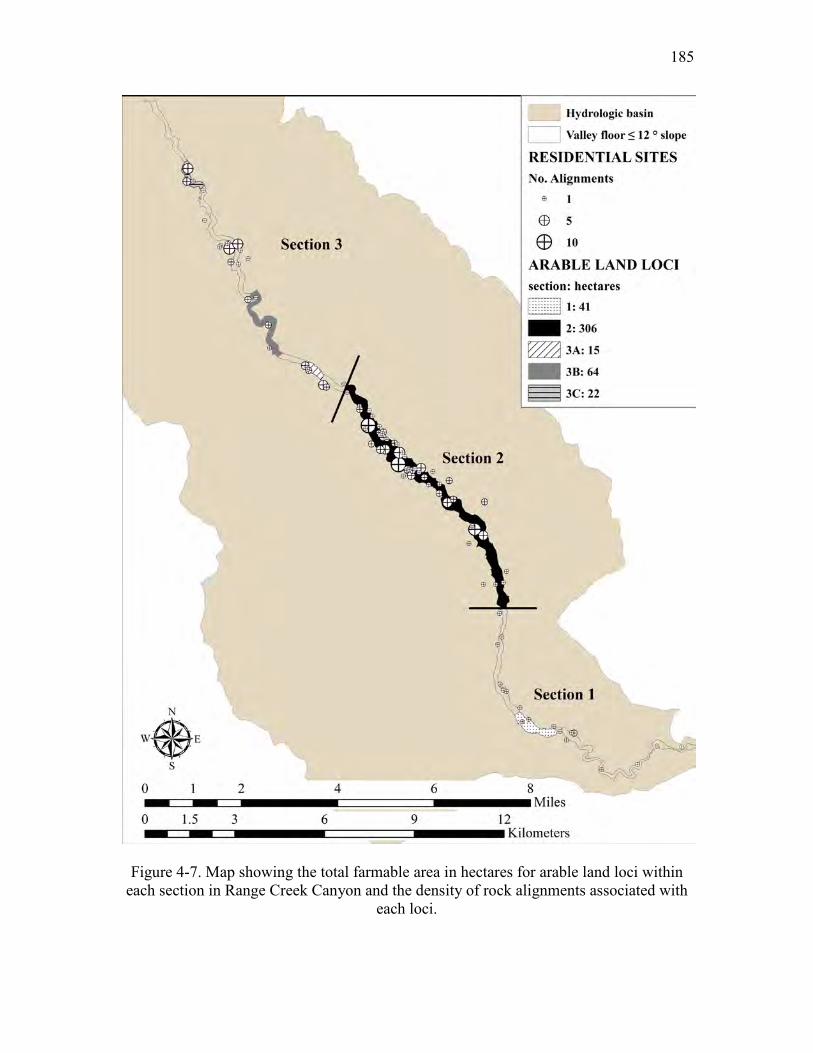
185
Figure 4-7. Map showing the total farmable area in hectares for arable land loci within each section in Range Creek Canyon and the density of rock alignments associated with
each loci.

CHAPTER 5
FUTURE RESEARCH
The data presented in the preceding chapters offer many insights into the
environmental opportunities and constraints faced by Fremont farmers in Range Creek
Canyon. Most importantly, dry farming was unlikely to have been a successful strategy
anytime during the major period of Fremont occupation of Range Creek Canyon, AD
900-1200. To some degree, the results might apply more generally to the West Tavaputs
Plateau as a whole, but care needs to be exercised. Utah is a land of extreme topography.
The entire water cycle can be viewed from the benches of Salt Lake City where the Great
Salt Lake and the snowpack in the Wasatch Mountain can be seen by simply turning
one’s head. The methods and approach outlined in the preceding chapters can be
conducted anywhere, and anyone interested in prehistoric farming in a different part of
the arid or semi-arid Southwest are encouraged to following them.
It is also worth stressing that the strength of the conclusions of this research is
firmly rooted in the dendroclimatological results presented by Knight et al. (2010).
Without these data, which allowed me to empirically link the results of the farming
experiments to the prehistoric period of interest, the conclusions of my research would
have been much more qualified with a lot of “all else being equal” and a lot of
assumptions about the relationship between the modern climate and that of the past.

187
While not directly archaeological in character, these paleoenvironmental reconstructions
are the life-blood of modern, ecologically-oriented archaeological research.
As is always true, I am left with more questions than I answered. What is it about
the arable land loci that made them more suitable for farming: an economy of scale, the
costs of irrigation, social factors, or other ecological factors? Investigating the costs of
irrigation, the hydrology of the creek, and the fluvial history of the canyon may answer
these questions.
Irrigation Cost
The first, and I think most important, research we need to undertake is the
investigation of the other half of the equation in the cost/benefit analysis of simple
irrigation farming. The analyses presented here made the benefits clear: more water
equals higher yields. When combined with the ability to control the timing of irrigation
events relative to the growth and development of the maize crop, irrigation also reduces
many of the risks associated with farming. As I stated earlier, when the benefits
outweigh the costs, in the context of the opportunity costs associated with farming, we
should expect prehistoric peoples to consider irrigation a viable strategy for dealing with
precipitation shortfalls in an arid or semi-arid environment. If the costs of irrigation were
higher than the benefit, we would expect the Fremont to abandon maize farming in an
environment like Range Creek Canyon, where precipitation thresholds for dry farming
have not been reached over the last 30 years and rarely attained during the 300-year
Fremont occupation. The amount of archaeological evidence for farming in Range Creek

188
Canyon tells us that they were farming despite low precipitation which leads us to believe
they used irrigation despite the costs, which were undoubtedly quite high.
What is missing is a similar experimental study to quantify the costs of irrigation
in Range Creek Canyon. One recent study, conducted on the flanks of Boulder Mountain
in central Utah, estimated the costs of digging an irrigation ditch with simple technology
in an area where prehistoric irrigations were noted (Kuehn 2014). Kuehn obtained
extremely high costs in this setting: construction is estimated to have cost 6,930 total
person hours with maintenance costs ranging between 4,140 and 12,269 total person
hours (Kuehn 2014: Table 10, p78). We anticipate that these costs are on the very high
end of the distribution since they were digging in rocky, shallow soils quite unlike the
alluvial sediments along Range Creek. Only experimentation in Range Creek Canyon
will tell.
In order to quantify the costs of irrigation in Range Creek Canyon, we plan to
build our own simple surface irrigation system. The simple irrigation system will include
a single diversion dam and a single ditch situated to water an area large enough to plant
another experimental maize plot. A detailed contour map of the area will be made to
understand how water can be most efficiently applied to the most area for our investment.
The construction technique will include only materials and tools available to the Fremont.
The time and energy required to build the system will be recorded and will include age
and gender which likely will affect efficiency. The experiment will be designed to
capture participants “learning curves,” how they improve over time as they learn the most
efficient ways to excavate ditches, move dirt, gather materials, and build dams using only

189
simple technology. We hope to use the water from the creek to assist in the choice of
ditch location and in the movement of dirt along the ditch after irrigation has started.
Once our irrigation system is operational, we will plant a second experimental
maize farm and record ongoing maintenance and operational costs associated with
irrigating with the system we built. Because of the time required to construct the
irrigation system, this second crop might be planted too late in the season to reach full
maturity, but the costs of using and maintaining the irrigation ditches will be an important
baseline for future research. The field will be mapped each year to record the impacts due
to use and other environmental impacts such as flooding events. What is so interesting
about irrigation is that the capital investments in the first year or two might be very high,
but we suspect the costs of maintaining it are lower than the initial investment. By paying
the larger costs up front, the amortized annual capital costs decrease with increased use-
life or life-expectancy.
Once we quantify the costs of irrigating a small area of Range Creek, we will
expand the experiment to other areas of the canyon to ascertain how local topography,
soils, hydrology and extant vegetation influence those costs. With these data, we can
then model how variation in the local environment influences the ratio of costs and
benefits across the farmable floor of Range Creek Canyon. We suspect, but have not
demonstrated, that irrigation will be more expensive the narrower areas in Section 3 that
are interrupted by ridgelines relative to the costs of irrigating the larger, uninterrupted
areas in Section 2 (see Chapter 5). Knowing the time and energy expenditure associated
with constructing each part of the irrigation system (dam, ditch, and other water-control
features) will allow us to estimate any economies of scale for different sized fields in

190
similar environmental situations. For example, what are the differences in costs
associated with irrigating a hectare of land when only one diversion dam and one canal
are needed versus a hectare of land requiring two diversions and two ditches? Three
ditches? We anticipate that modeling the costs and benefits of irrigation in various areas
of the canyon will better explain the pattern of clustering in Fremont residential sites.
Differences in the costs of irrigation in each section might explain the higher density
populations in Section 2 and loci 3a and 3c verses 3b.
Hydrology
Employing surface irrigation for farming requires access to a reliable source of
water during the growing season. Farmers must have access to the amount of water
needed to maintain sufficient field soil moisture, requiring that it be irrigated multiple
times during the growing season semi-arid environments. Much of the research
presented in Chapter 3 was designed to understand the relationship between the amount
of irrigation water applied and the size of the resulting harvest. The important conclusion
from that research is that additional water (within reason) above what is needed to bring a
crop to harvest is beneficial because it will increase the size of that harvest.
Volume is the critical variable when it comes to irrigation. How much water does
the creek carry and how does that vary as a function of time (annual and seasonal
variation) and space (variation along its length). While annual fluctuations in streamflow
are largely a function of annual variation in precipitation within the watershed, in areas
with significant topographic relief within the watershed, seasonal variance in
precipitation is also a major factor because it determines whether precipitation is cached

191
at higher elevations as snow or whether it enters the system much more quickly as rain.
Seasonal variance in streamflow is obviously also a function of the seasonal patterns of
precipitation, but seasonal temperatures also plays a role. Variation in streamflow along
its length is largely a function of subtractive processes like evaporation and percolation,
but can also vary as a function of inputs of groundwater along the stream course. All of
these factors come into play in determine how much streamflow is present in a particular
time at a particular place along Range Creek.
We are proposing that, during the height of the Fremont occupation of Range
Creek Canyon, that they practiced some form of surface irrigation by diverting water
from the creek to irrigate their fields of maize. This is likely to be a much more
significant subtractive process than, say, evaporation, and its effect on streamflow at and
below the point of diversion would be important. The rate at which water from the creek
will be diverted from the creek will be a function of the number and size of the fields that
are being irrigated, and the diversion locations will be a function of the location of the
fields within the drainage.
Range Creek is not a large creek. During heavy spring-runoff it can be a couple
of feet deep and 6-10 ft (1.5-3 m) wide. This period of runoff typically occurs in May
and June, after which the steamflow drops markedly. By late summer and early fall, the
creek is down to a trickle in many places, a couple of inches deep and only a couple of
feet wide. We suspect that some stretches of Range Creek maintain streamflow better
than others during dry periods due to the inflow of groundwater. So even without the
subtractive effects of irrigation, we suspect that some stretches of the creek are more
conducive for irrigation than others, especially during dry periods.

192
Beginning in 2015, we will systematically measure the streamflow from the
northern boundary of the field station to the confluence of Range Creek with the Green
River. Monitoring stations will be established about every kilometer along this stretch of
the creek, and once a month the streamflow will be calculated at each monitoring station.
This will be accomplished by using a portable Valeport Model 801 Flow Meter. This
electromagnetic flow meter allows recording the current in very shallow water (>5 cm), a
necessity for obtaining multiple estimates of the current at each stream cross-section.
When combined with depth of water measurements, an estimate of streamflow can be
calculated.
It may require several years before temporal and spatial patterning in the
streamflow of Range Creek will be evident, and decades before a sufficient set of
samples are collected to quantitatively model the hydrological system, but we have every
reason to believe that some of the mismatches between expected densities of rock
alignments and size of arable land will be resolved with this information. If some
sections of the creek routinely have lower stream flows than others during dry years, then
placing fields requiring diversions in these sections should be a high risk option.
Fluvial History
While looking at the current shape and course of the creek is an excellent starting
point for understanding the costs of diverting water for irrigation, documenting
meanderings in the creek over time and any major episodes cutting and filling will be
crucial to understanding the Fremont farming landscape. The creek location is important
for understanding the length of the ditches needed to irrigate fields in different locations.

193
Understanding the fluvial cut-fill dynamics is important to understanding the costs
associated with constructing diversion dams. Needless to say, constructing a diversion
dam capable of lifting the water 3 meters vertically is likely to be much more expensive
than constructing a diversion in a streambed that is only a meter below the mouth of the
field ditch. Recent research in Range Creek by Rittenour et al. (2015) indicates that cut-
fill sequences were likely important, at least in some sections of the canyon. Based on
their study employing optically stimulated luminescence for dating, that the creek was as
entrenched as it is today prior to about A.D. 1130 + 130. At or before that time, the
floodplain began to aggrade, perhaps by as much as 3.5 m, until about AD 1350 +170,
when it may have witnessed another episode of entrenchment of as much as 2.5 m
(Rittenour et al. 2015:73). Further work will be required to determine the spatial and any
temporal variability in this sequence.
Maize Farming Experiments
We will continue the maize farming experiments. Each year will add another
sample to our dataset so that we can monitor the yearly variation in farming returns. We
will continue to plant Tohono O’odham maize for several years and plant it in the same
layout within the plots to maintain comparable results for multiple years. Over time this
will allow us to generate error estimates for the relationship between irrigation water
applied and increases in harvest yield. Several experimental changes will be implemented
to investigate questions that arose from the results of the 2014 experiment. We plan to fill
in the gap in the irrigation schedule between Plot 1 (one irrigation event) and Plot 2 (eight
irrigation events) to determine the minimum amount of water need to produce at least

194
some maize. We also plan to add additional irrigation events beyond the 18 used in Plot 4
to extend the function beyond this point to determine when additional water does not
affect, or has a negative effect, on the yield (Figure 5-1).
For the 2015 growing season we will plant six plots. The watering schedule will
be as follows: Plot1 not irrigated, Plot 2 irrigated once every 3-4 weeks, Plot 3 irrigated
once every 2 weeks, Plot 4 irrigated once per week, Plot 5 irrigated twice per week, and
Plot 6 irrigated every day. By watering one of the plots only every 3-4 weeks, we can test
whether it is possible to get a yield at all with fewer than the 8 irrigations that we started
with as our lower end. By adding a plot that will be watered every day, we will test
whether it is possible to add too much water.
Soil Moisture Sensors
The 2014 results generated questions about rooting depth of dry adapted maize
varieties and moisture availability in the upper section of the soil profile. This summer
we will place soil moisture sensors at 6 in the experimental farm plots to record
fluctuations in soil moisture above 12 in (the depth of our shallowest sensors in 2014).
We suspect the available moisture above 12 in (30 cm) was being depleted more quickly
than the lower sensors could track. The Tohono O’odham maize roots seemed unable to
pull moisture from the reservoir of available water evident from the sensor readings at 12
in (30 cm) and 30 in (76 cm). We will also place several more shallow sensors in the
control plot to capture changes in available moisture at 4 inches (10 cm) below surface.

195
Rooting Depth
Rooting depth of dry adapted heirloom varieties of maize are poorly understood
(Benson 2010:5). During the 2014 season, only one basin was excavated to examine the
root system and to measure the depth of the tap roots. At the end of the next growing
season, we will compare rooting depth in all plots by excavating a basin from each plot. It
is typical for 75% of the root system to be in the upper half of the total rooting depth
(Benson 2010: 5). There is evidence from the agronomy literature on the rooting depth of
modern hybrid maize that suggests the amount of water available can affect the depth at
which tap roots will extend into the soil profile, i.e., with less surface water available,
roots extend deeper (Shaw 1988:621) The packets that accompanied the Tohono
O’odham seeds used in the Range Creek experiments suggested that it be planted 1 inch
below the surface but we later found ethnographic evidence that the seeds of Tohono
O’odham maize should be planted at 6 in (15 cm) below the ground surface (Castetter
and Bell 1942; Muenchrath 1995). Had we planted the seeds deeper, the roots would have
extended deeper into the soil profile. Whether or not we should change the planting depth
at this point in the experiment is unclear, but it might be worth experimenting with deeper
planting in the future.
Other Avenues
In addition to tracking aspects of rooting depth and increasing the number of
sensors tracking soil moisture availability, we plan to improve the frequency and details
pertaining to the documentation of the growth cycle of the maize in each irrigation cycle.
By tracking the development of each plant we can better understand the variation in

196
development within and between plots compared to the Cumulative Growing Degree
Days.
With this being our second year planting in the same location, it is a good time to
start tracking organic nitrogen depletion and changes in salinity caused by repeated
irrigation. The depletion of nitrogen over time can have devastating effects on the
productivity of crops (Benson et al. 2013:2872) requiring nitrogen fixers such as bean
plants, to replenish the soil for healthy maize crop production. Repeated irrigation can
lead to increases in soil salinity, measured in electrical conductivity. Conductivity above
1.5 dS/m can cause declines in maize productivity (Benson 2010: Figure 8). Future
experiments conducted in the same field in Range Creek Canyon will be able to track
changes in the soil for a better understanding of what the Fremont farmers would have
been dealing with as far as the length of time they could occupy and irrigate a farm field
before organic nitrogen was depleted or salinity levels became too high.
Discussion
The advent of food production, in this case farming, was a major inflection point
in the course of the human experience. It is associated with a variety of behavioral and
material consequences, such as increased sedentism (construction of more substantial
dwellings and the generation of larger amounts of refuse), increase in population
densities (more and larger archaeological sites), and a more diverse material culture. In
some areas of the world, food production led to the development of state-level societies,
with urban centers, craft specialization, monumental architecture, writing and the suite of
features often considered the hallmark of civilizations.

197
The Fremont provide an important opportunity for understanding the process of
adopting farming as part of a larger subsistence strategy that was not only accepted, but at
a later date rejected. As demonstrated so clearly by Barlow (1997 and 2002), viewing
farming as a sequence of activities within the context of the costs and benefits of those
activities, as well as within the broader context of the alternatives, is a powerful tool for
exploring this transformative event. Fully fleshing out the local costs and benefits will
require experimentation similar to that presented here and anticipated in the future at the
Range Creek Field Station. It will also require problem-oriented ethnographic research to
elucidate the costs and benefits of the full suite of farming strategies employed
historically and by modern cultures. And it will require placing these data into the
context of humans making rational decisions in terms of the opportunities and constraints
of the local natural and social environment.
The benefits of conducting this type of research at a field station are
immeasurable. Archaeologists rarely have the opportunity to repeat experiments year
after year in a setting that offers such rich archaeological record and paleoenvironmental
archives for reconstructing the past. The results from ongoing experiments recording both
the costs and benefits of irrigation will have a lasting impact on the way that we think
about maize farming in semi-arid environments and in understanding how the Fremont
negotiated the tradeoffs in their substance strategies.

198
Figure 5-1. Example of the areas of the returns curve from the 2014 experimental maize plots that need to be explored further with additional plots and changes in the
irrigation schedule. A plot will be added that is watered once every 3-4 weeks, and a plot will be added that is watered every day to test whether yield begins to diminish.

REFERENCES
Adams, Karen R. 2004 Anthropogenic Ecology of the North American Southwest. In People and
Plants in Ancient Western North America, edited by Paul E. Minnis, pp. 167-204. Smithsonian Books, Washington.
Adams, Karen R. and Kenneth L. Peterson
1999 Environment. In Colorado Prehistory: A Context for the Southern Colorado River Basin, edited by William D. Lipe, Mark D. Varien and Richard H. Wilshusen, pp. 14-58. Crow Canyon Archaeological Center, Cortex Colorado. Colorado Council of Professional Archaeologists.
Adams, Karen R., Deborah A. Muenchrath, and Dylan M. Schwindt
1999 Moisture effects on the Morphology of Ears, Cobs and Kernels of a South-western U.S. Maize (Zea mays L.) Cultivar, and Implications for the Interpretation of Archaeological Maize. Journal of Archaeological Science 26:483-496.
Adams, Karen R., Cathryn M. Meegan, Scott G. Ortman, R. Emerson Howell, Lindsay C. Werth, Deborah A. Muenchrath, Michael K. O’Neill, Candice A. C. Gardner
2006 MAIS (Maize of American Indigenous Societies) Southwest: Ear Descriptions and Traits that Distinguish 27 Morphologically Distinct Groups of 123 Historic USDA Maize (Zea mays L. spp. Mays) Accessions and Data Relevant to Archaeological Subsistence Models. JSMF Grant # 21002035. Arizona State University, Tucson.
Afuakwa, Joe J. and R. Kent Crookston
1983 Using the Kernel Milk Line to Visually Monitor Grain Maturity in Maize, Crop Science, 24(4):687-691.
Afyuni, Majid M., D. Keith Cassel and Wayne P. Robarge
1993 Effect of Landscape Position on Soil Water and Corn Silage Yield, Soil Science Society of America Journal, 57(6):1573-1580.
Allen, Jim and James F. O’Connell

200
2008 Getting from Sunda to Sahul. In Islands of Inquiry: Colonization, Seafaring and the Archaeology of Maritime Landscapes, edited by Geoffrey Clark, Foss Leach and Sue O’Connors, pp.31-46. AMU E Press, Canberra, Australia, Terra Australis.
Anderson, Edgar 1954 Maize of the Southwest. Landscapes 3(2):26-27. Andrade F. H., L. Echarte, R. Rizzalli, A. Della Maggiora and M. Casanovas
2000 Kernel Number Prediction in Maize under Nitrogen or Water Stress Agronomy Journal 42(4):1173-1179
Arnold, Shannon, Jamie Clark, Rachelle Green, and Duncan Metcalfe
2007 Report of the 2007 Survey and Excavation at Range Creek Canyon, Utah. Manuscript on file at the Natural History Museum of Utah and the Antiquities Section of the Utah Division of State History, Salt Lake City, Utah.
2008 Report of the 2008 Survey and Excavation at Range Creek Canyon, Utah. Manuscript on file at the Natural History Museum of Utah and the Antiquities Section of the Utah Division of State History, Salt Lake City, Utah.
Arnold, Shannon, Katie Green, Corinne Springer, and Duncan Metcalfe
2009 Report of the 2009 Survey and Excavation at Range Creek Canyon, Utah. Manuscript on file at the Natural History Museum of Utah and the Antiquities Section of the Utah Division of State History, Salt Lake City, Utah.
2011 Report of the 2010 Survey and Excavation at Range Creek Canyon, Utah. Manuscript on file at the Natural History Museum of Utah and the Antiquities Section of the Utah Division of State History, Salt Lake City, Utah.
Barlow, K. Renee
1997 Foragers that Farm: A Behavioral Ecology Approach to the Economics of Corn Farming for the Fremont Case. PhD Dissertation, University of Utah, Salt Lake City.
2002 Predicting Maize Agriculture among the Fremont: An Economic Comparison of Farming and Foraging in the American Southwest. American Antiquity 67(1):65-88.
Barlow, K. Renee and Duncan Metcalfe
1996 Plant Utility Indices: Two Great Basin Examples. Journal of Archaeological Science 23:351-371.
Beck, R. Kelly
2008 Transport Distance and Debitage Assemblage Diversity: An Application of the Field Processing Model to Southern Utah Toolstone Procurement Sites. American Antiquity 73:759-780.

201
Bellorado, Benjamin A. 2007 Breaking Down the Models: Reconstructing Prehistoric Subsistence
Agriculture in the Durango District of Southwestern Colorado. Unpublished M.A. dissertation, Department of Anthropology, Northern Arizona University, Flagstaff.
Benson, Larry V., Kenneth L. Petersen, and John Stein
2007 Anasazi (Pre-Columbian Native American) Migrations during the Middle-12th and Late-13th Centuries-Were they Drought Induced? Climate Change 83(1-2):187-213.
Benson, Larry V. and Michael S. Berry
2009 Climate Change and Cultural Response in the Prehistoric American Southwest, USGS Staff--Published Research. Paper 725.
Benson, Larry V.
2010a Factors Controlling Pre-Columbian and Early Historic Maize Productivity in the American Southwest, Part 1: The Southern Colorado Plateau and Rio Grande Regions, Journal of Archaeological Method and Theory, 18: 1-60.
2010b Factors Controlling Pre-Columbian and Early Historic Maize Productivity in the American Southwest, Part 1: the Chaco Halo, Mesa Verde, Pajarito Plateau/Bandelier, and Zuni Archaeological Regions, Journal of Archaeological Method and Theory, 18:61-109.
Benson, Larry V., D. K. Ramsey, David W. Stahle, Kenneth L. Petersen
2013 Some Thoughts on the Factors that Controlled Prehistoric Maize Production in the American Southwest with Application to Southwestern Colorado. Journal of Archaeological Science 40:2869-2880.
Bettinger, Robert L.
1991 Settlement Data and Subsistence Systems. American Antiquity 46:640-643.
Binford, Lewis R.
1980 Willow Smoke and Dogs' Tails: Hunter-Gatherer Settlement Systems and Archaeological Site Formation. American Antiquity, 45(1):4-20.
Bird, Douglas W. and James F. O’Connell
2006 Behavioral Ecology and Archaeology. Journal of Archaeological Research 14:143-188.
Boomgarden, Shannon A., Darrin Day, Isaac Hart, Alexa Hudson, Erik Martin, Duncan Metcalfe, Corinne Springer, and Katie Thomas
2013 Report of the Archaeological Investigations in Range Creek Canyon, Utah: University of Utah Archaeological Field School 2011-2012. Manuscript

202
on file at the Natural History Museum of Utah and the Antiquities Section of the Utah Division of State History, Salt Lake City, Utah.
Boomgarden, Shannon A., Corinne Springer, Duncan Metcalfe, and Andrew Yentsch
2014 Report of the Archaeological Investigations in Range Creek Canyon, Utah: University of Utah Archaeological Field School 2013. Manuscript on file at the Natural History Museum of Utah and the Antiquities Section of the Utah Division of State History, Salt Lake City Utah.
Boomgarden, Shannon A.
2009 An Application of ArcGIS Viewshed Analysis in Range Creek Canyon, Utah. Utah Archaeology 22(1), pp. 15-30.
Boomgarden, Shannon A., Duncan. Metcalfe, and Corinne Springer
2014 Prehistoric Archaeology in Range Creek Canyon, Utah: A Summary of Activities of the Range Creek Field Station. Utah Archaeology 27(1):9-32.
Boyer J. S. and Mark E. Westgate
2004 Grain Yields with Limited Water. Journal of Experimental Botany 55(407):2385-2394.
Castetter, Edward F. and Willis H. Bell
1942 Pima and Papago Indian Agriculture. University of New Mexico Press, Albuquerque NM.
Clausnitzer, V. and Jan W. Hopmans
1994 Simultaneous Modeling of Transient Three-dimensional Root Growth and Soil Water Flow. Plant and Soil 164(2):299-314
Classen, M. and Robert H. Shaw
1970 Water Deficit Effect on Corn. I. Grain Components. Agronomy Journal 62(5):652-655.
Codding, Brian F. and Terry L. Jones
2013 Environmental Productivity Predicts Migration, Demographic, and Linguistic Patterns in Prehistoric California. PNAS 110(36):14569-14573.
Coltrain, Joan
2011 Evidence for Fremont Maize Farming in the Soil Organic Chemistry of Range Creek Canyon. Paper presented at the 76th Annual meetings of the Society of American Archaeology, Sacramento CA.
Daly, Christopher, Michael Halbleib, Joseph I. Smith, Wayne P. Gibson, Matthew K. Doggett, George H. Taylor, Jan Curtis and Phillip P. Pasteris

203
2008 Physiographically sensitive mapping of climatological temperature and precipitation across the conterminous United States. International Journal of Climatology, 28:2031-2064
Daly, Chistopher and Kirk Bryant
2013 The PRISM Climate and Weather System-An Introduction. Online http://prism.oregonstate.edu/documents/PRISM_history_jun2013.pdf
Day, Paul R.
1965 Particle fractionation and particle-size analysis. In Methods of Soil Analysis, edited by C. A. Black, D. D. Evans, J. L. White, L.E. Ensminger, and F.E. Clark, pp. 545-567. Agronomy Monograph No. 9 (1st edition). American Society of Agronomy/Soil Science Society of America, Madison, WI.
Denmead, Owen T. and Roger H. Shaw
1962 Availability of Soil Water to Plants as Affected by Soil Moisture Content and Meteorological Conditions. Agronomy Journal 54(5):385-390.
Duley, Frank L.
1939 Surface Factors Affecting the Rate of Intake of Water by Soils. Soil Sci. Soc. Am. Proc. 4:60-64
Duley, Frank L. and Latimer L. Kelly
1939 Effect of Soil Type, Slope and Surface Conditions on Intake of Water. Nebr. Agr. Col. Expt. Sta. Res. Bull. 112.
Dyson-Hudson, Rada and Eric A. Smith
1978 Human Territoriality: An Ecological Reassessment. American Anthropologist 80(1):21-41.
Fageria, Nand K., Virupax C Baligar and Ralph B. Clark,
2006 Physiology of Crop Production. Waworth Press Inc, Binghamton. Fretwell, Stephen
1972 Populations in a Seasonal Environment, Princeton University Press, Princeton NJ.
Garcia y Garcia, Axel, M. A. Abritta, Cecilia M. Tojo Soler, and A. Green
2014 Water and Heat Stress: The Effect on the Growth and Yield of Maize and the Impacts on Irrigation Water. In Sustainable Irrigation and Drainage V: Management, Technologies, and Policies, edited by Carlos A. Brebbia and Henning Bjornlun, pp. 77-87 . WIT Press, Southampton, UK.
Gee, Glendon W. and James W. Bauder

204
1986 Particle-size Analysis. In Methods of Soil Analysis, edited by A. Klute. pp. 383-412. Agronomy Monograph No. 9 (2nd edition). American Society of Agronomy/Soil Science Society of America, Madison, WI.
Gillen, John
1938 Archaeological Investigations in Nine Mile Canyon. Bulletin of the University of Utah 28(11). Salt Lake City.
Grayson, Donald K.
1993 The Desert’s Past: A Natural Prehistory of the Great Basin. Smithsonian Institute Press: Washington.
Haegele, Jason W.
2008 Maize (Zea mays L.) Kernel Development, Suitability for Dry-grind Ethanol Production, and Susceptibility to Aflatoxin Accumulation in Relation to Late Season Water Stress. MA Thesis, Iowa State University.
Hanway, Donald G.
1966 Irrigation. In Pierre, W.H. (ed.) Advances in Corn Production: Principles and Practices, pp. 155-176, Iowa State University Press, Ames.
Hard, Robert J. and William L. Merrill
1992 Mobile Agriculturalists and the Emergence of Sedentism: Perspectives from Northern Mexico. American Anthropologist 93(3):601-620.
Hund, Andreas, Nathinee Ruta, and Markus Liedgens
2009 Rooting depth and water use efficiency of tropical maize inbred lines, differing in drought tolerance. Plant Soil 318:311-325.
Hunt, Eric D., Mark Svoboda, Brian Warlow, Kenneth Hubbard, Michael Hayes, Tim Arkebauer
2014 Monitoring the Effects of Rapid Onset of Drought on Non-irrigated maize with Agronomic Data and Climate-based Drought Indices. Agricultural and Forest Meteorology 191:1-11.
Irrometer® Company, Inc.
2013 Recommendations-Sensor Interpretations http://www.irrometer.com/pdf/supportmaterial/949%20Sensor%20Interpretation-WEB.pdf
Janetski, Joel C., Mark L. Bodily, Bradley A. Newbold, and David T. Yoder
2012 The Paleoarchaeic to Early Archaic Transition on the Colorado Plateua: The Archaeology of North Creek Shelter. American Antiquity 77(1):125-159.
Jones, Kevin T.

205
2010 Vanished, Collapsed, and Abandoned-Some Inconvenient Truths Regarding the Demise of the Fremont. Paper presented at the 32rd Great Basin Anthropological Conference. Layton, UT.
Jones, Kevin T. and Shannon A. Boomgarden
2012 Thieving Neighbors, Marauding Clans, or Warring Tribes: An Evolutionary Approach to Fremont Conflict. Paper presented at the 33rd Great Basin Anthropological Conference, Stateline, NV.
Kennett, Douglas J.
2005 The Island Chumash: Behavioral Ecology of a Maritime Society. University of California Press, Berkeley.
Kennett, Douglas J., Atholl J. Anderson, Bruce Winterhaulder,
2006 The Ideal Free Distribution, Food Production, and the Colonization of Oceania, in Behavioral Ecology and the Transitions to Agriculture. Edited by Douglas Kennett and Bruce Winterhaulder, pp. 265-288. University of California Press, Berkeley.
Knight, Troy A., David M. Meko, Christopher H. Baisan
2010 A Bimillenial-length Tree-ring Reconstruction of Precipitation for the Tavaputs Plateau, Northeastern Utah. Quaternary Research, 73(1):107-117.
Kramer, Paul J.
1969 Plant and Soil Water Relationships: A Modern Synthesis. McGraw-Hill Book Co. Inc. New York.
Kuehn, Chimalis R.
2014 The Agricultural Economics of Fremont Irrigation: A Case Study from South-central Utah. Unpublished M.S. Thesis, Department of Anthropology, Utah State University, Logan Utah.
Lohse, Ernest S.
1980 Fremont Settlement Pattern and Architectural Variation. In Fremont Perspectives, edited by David B. Madsen, pp. 41-54. Antiquities Section Selected Papers 7(16).
Madsen, David B. and Steven R. Simms
1998 The Fremont Complex: A Behavioral Perspective. Journal of World Prehistory 12:255-336.
McMaster, Gregory S. and W. W. Wilhelm
1997 Growing Degree-Days: One Equation, Two Interpretations, Agricultural and Forest Meteorology 87:291-300
Metcalfe Duncan

206
2008 Range Creek Canyon. In The Great Basin: People and Place in Ancient Times, edited by Catherine S. Fowler and Don D. Fowler, pp. 117-123. School of Advanced Research Press, Santa Fe.
2011 Time in Range Creek. Symposium: Archaeology and Paleoecology in Range Creek Canyon, Utah. Paper presented at the 76th Annual Meeting of the Society for American Archaeology. Sacramento.
Metcalfe, Duncan and Lisa V. Larrabee
1985 Fremont Irrigation: Evidence from Gooseberry Valley, Central Utah. Journal of California and Great Basin Anthropology 7(2):244-254.
Metcalfe, Duncan, K. Renee Barlow, Jerry D. Spangler, and Corinne Springer
2005 Proposal for Archaeological and Ecological Investigations in Range Creek Canyon, 2005. Research Design on file at the Natural History Museum of Utah, Salt Lake City, Utah.
Metcalfe, Duncan and K. Renee Barlow
1992 A Model for Exploring the Optimal Trade-off between Field Processing and Transport. American Anthropologist 94:340-356.
Morss, Noel
1931 The Ancient Culture of the Fremont River in Utah. Peabody Museum of American Archaeology and Ethnology 12(3). Harvard University, Cambridge, Massachusetts.
Muenchrath, Deborah A.
1995 Productivity, Morphology, Phenology, and Physiology of a Desert-Adapted Native American Maize (Zea mays L.) Cultivar. Ph.D. Dissertation, Department of Agronomy, Iowa State University, Ames Iowa.
Muenchrath, Deborah A. and Ricardo J. Salvador
1995 Maize Productivity and Agroecology: Effects of Environment and Agricultural Practices on the Biology of Maize. In Soil, Water, Biology, and Belief in Prehistoric and Traditional Southwestern Agriculture, edited by H. Wolcott Toll, pp. 303-333. New Mexico Archaeological Council Special Publication 2.
Muenchrath, Deborah A., Maya Kuratomi, Jonathan A. Sandor, and Jeffrey A. Homburg
2002 Observed Study of Maize Production Systems of Zuni Farmers in Semiarid New Mexico. Journal of Ethnobiology 22(1):1-33.
Musick, J. T. and D. A. Dusek
1980 Irrigated Corn Yield Response to Water. Transactions of the ASAE 23:92-98.
National Engineering Handbook

207
1991 Irrigation, Section 15, United States Department of Agriculture, Soil Conservation Service (2nd edition).
Neild, Ralph E. and James E. Newman
1990 Growing Season Characteristics and Requirements in the Corn Belt. National Corn Handbook NCH 40. Purdue University, Cooperative Extension Service.
Netting, Robert
1972 Of Men and Meadows: Strategies of Alpine Land Use. Anthropological Quarterly, Dynamics of Ownership in Circum-Alpine Area (special issue) 45(3):132-144.
Nielson, Robert L.
2009 Interpreting Corn Hybrid Maturity Ratings. Corny News Network, Purdue University Department of Agronomy. Online http://www.kingcorn.org/news/timeless/HybridMaturity.html
2001 Grain fill stages in corn. Department of Agronomy, Purdue University, West Lafayette, IN. http://www.kingcorn.org/news/timeless/GrainFill.html.
Nurmiaty and Sumbangan Baja
2013 Spatial Based Assessment of Land Suitability and Availability for Maize (Zea mays L.) Development in Maros Region, South Sulawesi, Indonesia Open Journal of Soil Science, 3:244-251
O’Connell, James F. and Jim Allen
2012 The Restaurant at the End of the Universe: Modeling the Colonization of Sahul. Australian Archaeology 74:5-17.
Parsons, Jeffrey R.
1972 Archaeological Settlement Patterns. Annual Review of Anthropology 1:127-150.
Petersen, Kenneth L.
1985 The Experimental Gardens in Retrospect, Chapter 5. In Dolores Archaeological Program: Studies in Environmental Archaeology compiled by Kenneth L. Petersen, Vickie L. Clay, Meredith H. Matthews, and Sarah W. Neusius pp. 37-40. U.S. Department of the Interior, Bureau of Reclamation, Engineering and Research Center, Denver.
1988 Climate and the Dolores River Anasazi. University of Utah Anthropological Papers No. 113.
1994 A Warm and Wet Little Climatic Optimum and a Cold and Dry Little Ice Age in the Southern Rocky Mountains, U.S.A Climatic Change 26(2):243-269.

208
Petersen, Kenneth L., Vickie L. Clay, Meredith H. Matthews, Sarah W. Neusius, (compilers), and David A. Breternitz (principal investigator)
1985 Dolores Archeological Program: Studies in Environmental Archaeology, U.S. Department of Interior, Bureau of Reclamation, Engineering and Research Center, Denver.
Phillips, Phillip, James A. Ford, and James B. Griffin
1951 Archaeological Survey in the Lower Mississippi Alluvial Valley, 1940-47, Papers of the Peabody Museum 25. Cambridge Massachusetts.
Reagan, Albert B.
1930 Archaeological Notes on the Brush Creek Region, Northeastern Utah. Wisconsin Archaeologist 10:132-138.
Rhoads, Fred M. and C. Dean Yonts
1991 Irrigation Scheduling for Corn-Why and How, NCH-20 in National Corn Handbook, University of Wisconsin Extension (Electronic Version)
Rittenour, Tammy M., Larry L. Coats, and Duncan Metcalfe
2015 Investigation of Late and Post-Fremont Alluvial Stratigraphy of Range Creek, East-central Utah: Use of OSL When Radiocarbon Fails. Quaternary International 362:63-76.
Robins, J. S. and C. E. Domingo
1953 Some Effects of Severe Soil Moisture Deficits at Specific Growth Stages of Corn. Agronomy Journal 45:618-621.
Saini, Hargurdeep S. and Mark E. Westgate
2008 Reproductive Development in Grain Crops during Drought. Advances in Agronomy 68:59-96.
Setter, Tim L., Brian A. Flannigan, and Jeff Melkonian
2001 Loss of Kernel Set Due to Water Deficit and Shade in Maize. Crop Science 41(5):1530-1540.
Sharp, Robert E. and William J. Davies
1985 Root Growth and Water Uptake by Maize Plants in Drying Soil Journal of Experimental Botany 36 (9):1441-1456
Shaw, Rogert H.
1988 Climate Requirement. In Corn and Corn Improvement edited by G. F. Sprauge and J. W. Dudley, pp. 609-638,(3rd edition) American Society of Agronomy, Madison.
Shaw, Roger H. and J. E. Newman

209
1990 Weather and Stress in the Corn Crop. National Corn Handbook NCH 18. Purdue University, Cooperative Extension Service.
Shock, Clint C., Fen-Xin Wang, Rebecca Flock, Erik Feibert, Cedric A. Shock, and Andre Pereira
2013 Irrigation Monitoring Using Soil Water Tension, Sustainable Agriculture Techniques, EM 8900, Oregon State University, Extension Service
Shreve, Forrest
1934 Rainfall, Runoff, and Soil Moisture Under Desert Conditions. Annals of the Association of American Geographers 24:131-156.
Shuster, Rita
1983 Preliminary Report, Demonstration and Experimental Garden Studies, 1979 and 1980. Dolores Archaeological Program Technical Reports DAP-062. Final report submitted to the Bureau of Reclamation, Upper Colorado Region, Salt Lake City, in compliance with Contract No. 8-07-40-S0562.
Shuster, Rita and Robert A. Bye, Jr.
1981 Preliminary Results from the Dolores Archaeological Program Gardens. Part II of Developing an Integrated Model for Contemporary and Archaeological Agricultural Subsistence Systems. In Dolores Archaeological Program synthetic report, 1978-1981 DAP-055, pp235-251. Final report submitted to the Bureau of Reclamation, Upper Colorado Region, Salt Lake City, in compliance with Contract No. 8-07-40-S0562.
Simms, Steven R.
2012 The Archaeology of Fremont Irrigation: Pleasant Creek Utah. Presentation at the Utah Professional Archaeological Counsel Winter Meeting, Salt Lake City, Utah.
2008 Ancient Peoples of the Great Basin and Colorado Plateau. Left Coast Press, California.
Spangler, Jerry D.
2013 Nine Mile Canyon: The Archaeological History of an American Treasure. University of Utah Press. Salt Lake City, Utah.
Spangler, Jerry D., Duncan Metcalfe, and K. Renee Barlow
2004 Summary of the 2002-2003 Intuitive Surveys of the Wilcox Acquisition and Surrounding Lands, Range Creek Canyon. Utah Museum of Natural History Report of Investigations 03-1. Salt Lake City, Utah.
Spangler, Jerry D., Shannon A. Boomgarden, and Joel Boomgarden
2006 Chasing Ghosts: An Analysis of Vandalism and Site Degradation in Range Creek Canyon, Utah. Colorado Plateau Archaeological Alliance (http://www.cparch.org/index.html)

210
Spangler, Jerry D. 2013 Nine Mile Canyon: The Archaeological History of An American Treasure.
University of Utah Press, Salt Lake City. 2000 Radiocarbon Dates, Acquired Wisdom, and the Search for Temporal
Order in the Uinta Basin. In Intermountain Archaeology, edited by Madsen, Dave. B, and M.D Metcalf, pp. 88-99. University of Utah Anthropological Papers No. 122, University of Utah Press, Salt Lake City, UT.
Springer, Corinne and Shannon A. Boomgarden
2012 Lighthouse Wildfire Archaeological Survey Report. Natural History Museum of Utah Reports. Salt Lake City, Utah. Manuscript on file at the Natural History Museum of Utah and the Antiquities Section of the Utah Division of State History, Salt Lake City Utah.
Steward, Jullian H.
1938 Basin-Plateau Aboriginal Sociopolitical Groups. Bureau of American Ethnology Bulletin 120.
Talbot, Richard K. and Lane D. Richens
1996 Steinaker Gap: An Early Fremont Farmstead. Museum of Peoples and Cultures Occasional Papers No. 2, Brigham Young University, Provo Utah.
Thomas, David H.
1973 An Empirical Test for Steward’s Model of Great Basin Settlement Patterns. American Antiquity 38:155-176.
1983 The Archaeology of Monitor Valley: 1. Epistemology. Anthropological Papers of the American Museum of Natural History 58(1).
2008 Native American Landscapes of St. Catherines Island, Georgia. Anthropological Papers of the American Museum of Natural History 88(1-3).
Toll, H. Wolcott, Mollie S. Toll, Marcia L. Newren, and Wiliiam B. Gillespie
1985 Experimental Corn Plots in Chaco Canyon: The Life and Hard Times of zea mays L. In Environment and Subsistence of Chaco Canyon, New Mexico Publications in Archaeology 18E, Chaco Canyon Studies. edited by F. Joan Mathien, pp. 79-133. NPS USDI, Albuquerque, NM.
Trigger, Bruce G.
1989 A History of Archaeological Thought. Cambridge University Press, Cambridge, New York. USDA Natural Resources Conservation Service
2010 Soil Survey Manual Chapter 3: Examination and description of soils. Accessed online December 2014 at http://www.nrcs.usda.gov/wps/portal/nrcs/detail//?cid=nrcs142p2_054253
Van West, Carla R.

211
1996 Agricultural Potential and Carrying Capacity in Southwestern Colorado. A.D.901 to 1300. In The Prehistoric Pueblo World A.D. 1150-1350, edited by Michael A. Adler, pp. 214-228. University of Arizona Press, Tucson.
1994 Modeling Prehistoric Agricultural Productivity in Southwestern Colorado: A GIS Approach. Reports of Investigations 67. Department of Anthropology, Washington State University, Pullman and Crow Canyon Archaeological Center, Cortez.
Venkateswarlu, J.
2001 Management of Soils in Andhra Pradesh. Acharya N.G. Ranga Agricultural University, Hyderabad, Andhra Pradesh State, India.
Willey, Gordon R.
1953 Prehistoric Settlement Patterns in the Viru Valley, Peru. Bureau of American Ethnology Bulletin 155. Washington, D.C.
1956 Prehistoric Settlement Patterns in the New World. Viking Fund Publications in Anthropology No. 23, New York.
Wilde James D. and Guy L. Tassa
1991 A Woman at the Edge of Agriculture: Skeletal Remains from the Elsinore Burial Site, Sevier Valley, Utah. Journal of California and Great Basin Anthropology, 13(1).
Winterhaulder, Bruce
1981 Optimal Foraging Strategies and Hunter-gatherer Research in Anthropology: Theory and Models. In Hunter Gatherer Foraging Strategies: Ethnographic and Archaeological Analyse, edited by Winterhaulder, B. and E. A. Smith, pp. 13-36. University of Chicago Press, Chicago.
Winterhaulder, Bruce, Douglas L. Kennett, Mark N. Grote, and Jacob Batruff
2010 Ideal Free Settlement of California’s Northern Channel Islands. Journal of Anthropological Archaeology 29:469-490.
Yentsch, Andrew T., Joel C. Boomgarden, Shannon Arnold, and Jerry D. Spangler
2010 A Report of Archaeological Investigations in Range Creek Canyon, Utah: University of Utah Archaeological Field School 2005-2006. Manuscript on file at the Natural History Museum of Utah and the Antiquities Section of the Utah Division of State History, Salt Lake City, Utah.
Zeanah, David W.
1996 Predicting Settlement Patterns and Mobility Strategies: An Optimal Foraging Analysis of Hunter-Gatherer Use of the Mountains, Desert, and Wetland Habitats in the Carson Desert. Ph.D. Dissertation, Department of Anthropology, University of Utah.
2002 Central Place Foraging and Prehistoric Pinyon Utilization in the Great Basin. In Beyond Foraging and Collecting: Evolutionary Change in Hunter

212
Gatherer Settlement System, edited by Fitzhugh, B. and J. Habu Klewer, pp. 231-256. Academic/Plenum Publishers, New York.
2004 Sexual Division of Labor and Central Place Foraging Strategies: A Model for the Carson Desert of Western Nevada. Journal of Anthropological Archaeology 23:1-32.