Embed Size (px)
Citation preview

ALMA MATER STUDIORUM - UNIVERSITÀ DI
BOLOGNA
FACOLTA’ DI INGEGNERIA
CORSO DI LAUREA IN INGEGNERIA PER L’AMBIENTE E TERRITORIO
D.I.C.A.M.
TESI DI LAUREA
in
Idraulica Marittima M
EXPERIMENTAL INVESTIGATION OF THE
PERFORMANCE OF THE “ROLLING
CYLINDER” WAVE ENERGY CONVERTER
AND DESIGN OPTIMISATION
CANDIDATO: RELATORE:
Valeria Taraborrelli Prof.ssa Barbara Zanuttigh
CO-RELATORE:
Lucia Margheritini
Elisa Angelelli
Anno Accademico 2010/2011
Sessione III

1
INDEX
1. Introduction…………………………………………………………. 11
2. The wave energy resource…………………………………………. 13
2.1 General aspects of wave energy……………………………………... 15
2.2 Marine Energy and Wave Energy……………………………………. 17
2.3 Advantages and disadvantages of wave energy……………………… 31
2.4 Wave Energy in Europe……………………………………………… 34
3. Wave energy converters……………………………………………. 39
3.1 Location……………………………………………………………… 39
3.2 Type………………………………………………………………….. 43
3.3 Working principle……………………………………………………. 46
3.4 Development for WEC tests and developments……………………... 49
4. A new wave energy converter: the Rolling Cylinder……………... 57
4.1 Objectives of the experimental activity……………………………… 57
4.2 Aalborg Laboratory - The facility……………………………………. 57
4.3 The model……………………………………………………………. 62
4.4 Test program…………………………………………………………. 66
4.5 Description of the wave state………………………………………… 68
4.6 First measuring setup……………………………………………….... 69
4.7 Second measuring setup……………………………………………... 72
5. Power production and optimization of design parameters………. 75
5.1 Optimisation of fin thickness………………………………………… 75

2
5.2 Optimisation of the number of fin sets mounted on the model……… 79
5.3 Optimisation of the number of fins par set…………………………... 85
5.4 Optimisation of the best buoyancy level…………………………….. 90
5.5 Evaluation of the potential power production under regular waves…. 92
5.6 Evaluation of the power production under irregular waves………….. 95
6. Future development………………………………………………… 101
6.1 Shape and material of the fins……………………………………….. 101
6.1.1 Bio-fouling and marine antifouling coatings…………………….. 106
6.2 Moorings of the device………………………………………………. 111
6.3 Limit of the measuring setup and PTO (Power Take Off)…………... 112
6.4 Considerations of the environmental impact of wave energy devices 113
6.4.1 Interference with animal movements……………………………. 113
6.4.2 Navigation Hazard………………………………………………. 115
6.4.3 Noise during construction and operation………………………... 116
7. Example application in the Mediterranean Sea…………………... 119
7.1 Wave climate in Mazara del Vallo, Italy…………………………….. 120
7.2 Efficiency and yearly energy power production in Mazara del Vallo.. 120
7.3 Comparison between a hypothetical farm of Rolling Cylinder and
Wave Piston devices………………………………………………….
125
8. Conclusion…………………………………………………………... 133
Appendix…………………………………………………………….. 137

3
FIGURE INDEX
Figure 2.1: Wave power density around the world. The wave power
density is very variable around the world and its highest
values are detected in the Oceans between the latitudes of
30° and 60° on both hemispheres…………………………… 14
Figure 2.2: Main parameters of wave……………………………………. 19
Figure 2.3: Local fluid velocities and accelerations……………………... 22
Figure 2.4: Elliptical paths in shallow or transitional depth water and in
circular paths in deep water…………………………………. 22
Figure 2.5: The kinetic and potential energy of the wave energy……….. 26
Figure 2.6 : A spectrum…………………………………………………... 29
Figure 2.7 : Wave power density in Europe. In Europe the West coasts of
the U.K. and Ireland along with Norway and Portugal
receive the highest power densities………………………….. 34
Figure 3.1: Lateral section of a three-levels SSG device………………... 40
Figure 3.2: The steel OSPREY Design………………………………….. 41
Figure 3.3: The prototype ……………………………………………….. 43
Figure 3.4: Attenuator device: Pelamis wave farm……………………… 44
Figure 3.5: Point absorber device: OPT Powerbuoy…………………….. 45
Figure 1.6: Terminator device: Salter's Duck……………………………. 46
Figure 3.7: OWC: The Limpet…………………………………………... 47
Figure 3.8: Overtopping principle……………………………………….. 48
Figure 3.9: DEXA, an example of Wave Activate Body………………... 49
Figure 3.10: Location of Nissum Bredning in Denmark………………….. 50
Figure 4.1: Paddle system……………………………………………….. 58
Figure 4.2: Layout and section of the laboratory………………………... 58
Figure 4.3: Screen of the Awasys5………………………………………. 59
Figure 4.4: Screen of the WaveLab3.33 “Acquisition Data”……………. 60
Figure 4.5: Screen of the WaveLab3.33 “Reflection Analysis”…………. 61
Figure 4.6: Rolling Cylinder, drawing provided by developer………….. 63

4
Figure 4.7: Rolling Cylinder's prototype with 4 set of fins, 6 fins per
each set and thickness of the fins of 1 mm………………….. 63
Figure 4.8: Rolling Cylinder's prototype with 7 set of fins, 6 fins per
each set and thickness of the fins of 0,75 mm………………. 64
Figure 4.9: The full length model of the Rolling Cylinder device in the
laboratory of Aalborg University……………………………. 65
Figure 4.10: Different buoyancy levels………………………………….... 67
Figure 4.11: Potentiometer to measure the rotational speed……………… 70
Figure 4.12: Load cells to measure the force……………………………... 70
Figure 4.13: The measuring setup used to run the tests in irregular waves 71
Figure 4.14: Section of the device………………………………………… 73
Figure 5.1: Thickness 1………………………………………………….. 75
Figure 5.2: Thickness 0,75………………………………………………. 75
Figure 5.3: Thickness 0,4………………………………………………... 75
Figure 5.4: Representation of the efficiency for different values of the
torque, for the fin’s thickness of 0,4 mm, 0,75 mm and 1
mm. In the secondary axis there is the variation of
(angular velocity) with different values of the torque. This
graph is for the wave state 4 ( H= 0,113 m e T= 1,96 s)……. 76
Figure 5.5: Representation of the efficiency for different values of the
torque, for the fin’s thickness of 0,4 mm, 0,75 mm and 1
mm. In the secondary axis there is the variation of
(angular velocity) with different values of the torque. This
graph is for the wave state 5 (H=0,141 m e T=2,24 s)……… 76
Figure 5.6: Representation of the efficiency for different values of the
torque, for the fin’s thickness of 0,4 mm, 0,75 mm and 1
mm. In the secondary axis there is the variation of
(angular velocity) with different values of the torque. This
graph is for the wave state 6 (H=0,16 m e T=1,4 s)………… 77
Figure 5.7: Representation of the efficiency with the optimum load, for
the fin’s thickness of 0,4 mm, 0,75 mm and 1 mm………….. 78

5
Figure 5.8: Representation of the efficiency with the wave state, for the
fin’s thickness of 0,4 mm, 0,75 mm and 1 mm……………... 79
Figure 5.9: 7 set of fins mounted on the model………………………….. 80
Figure 5.10: 4 set of fins mounted on the model………………………….. 80
Figure 5.11: Representation of the efficiency for different values of the
torque, for different number of fins set mounted on the
model. In the secondary axis there is the variation of
(angular velocity) with different values of the torque. This
graph is for the wave state 3 (H = 0,085 m e T = 1,68 s)…… 81
Figure 5.12: Representation of the efficiency for different values of the
torque, for different number of fins set mounted on the
model. In the secondary axis there is the variation of
(angular velocity) with different values of the torque. This
graph is for the wave state 4 ( H= 0,113 m e T= 1,96 s)……. 81
Figure 5.13: Representation of the efficiency for different values of the
torque, for different number of fins set mounted on the
model. In the secondary axis there is the variation of
(angular velocity) with different values of the torque. This
graph is for the wave state 5 (H=0,141 m e T=2,24 s)……… 82
Figure 5.14: Representation of the efficiency for different values of the
torque, for different number of fins set mounted on the
model. In the secondary axis there is the variation of
(angular velocity) with different values of the torque. This
graph is for the wave state 6 (H=0,16 m e T=1,4 s)………… 82
Figure 5.15: Representation of the efficiency with the optimum load, for
different number of fins set mounted on the model (4 set, 7
set and 3 set)………………………………………………… 84
Figure 5.16: Representation of the efficiency with the wave state, for
different number of fins set mounted on the model (4 set, 7
set and 3 set)…………………………………………………
84
Figure 5.17: 6 fins par set…………………………………………………. 85
Figure 5.18: 3 fins par set…………………………………………………. 85

6
Figure 5.19: 3 fins par set alternate……………………………………….. 85
Figure 5.20: Representation of the efficiency for different values of the
torque, for different number of fins par set. In the secondary
axis there is the variation of (angular velocity) with
different values of the torque. This graph is for the wave
state 4 ( H= 0,113 m e T= 1,96 s)…………………………… 86
Figure 5.21: Representation of the efficiency for different values of the
torque, for different number of fins par set. In the secondary
axis there is the variation of (angular velocity) with
different values of the torque. This graph is for the wave
state wave state 5 (H=0,141 m e T=2,24 s)…………………. 87
Figure 5.22: Representation of the efficiency for different values of the
torque, for different number of fins par set. In the secondary
axis there is the variation of (angular velocity) with
different values of the torque. This graph is for the wave
state 6 (H=0,16 m e T=1,4 s)………………………………... 87
Figure 5.23: Representation of the efficiency with the optimum load, for
different number of fins par set (6 fins, 3 fins and 3 fins
alternate par set)……………………………………………... 89
Figure 5.24: Representation of the efficiency with the wave state, for
different number of fins par set (6 fins, 3 fins and 3 fins
alternate par set)……………………………………………... 89
Figure 5.25: Representation of the efficiency for different values of the
torque, for different level of buoyancy. In the secondary axis
there is the variation of (angular velocity) with different
values of the torque. This graph is for the wave state 5
(H=0,141 m e T=2,24 s)……………………………………... 90
Figure 5.26: Representation of the efficiency with the load, for different
buoyancy levels………………………………………………
91
Figure 5.27: Representation of the efficiency with the wave state 5, for
different buoyancy levels……………………………………. 92
Figure 5.28: Efficiency depending on the mean torque for different wave 95

7
conditions in scale 1:25………………………………………
Figure 5.29: Angular speed as function of the mean torque, for the tested
wave conditions with trend lines and corresponding
equations. Scale 1:25………………………………………... 96
Figure 6.1: A composite laminate cross section…………………………. 102
Figure 6.2 : A composite laminate……………………………………….. 103
Figure 6.3: Marine bio-fouling grew on a boat………………………….. 111
Figure 7.1: Position of the 14 Italian buoys……………………………... 119
Figure 7.2: Trend of the Irregular Danish Sea…………………………… 121
Figure 7.3: Trend of the Irregular Italian Sea……………………………. 121
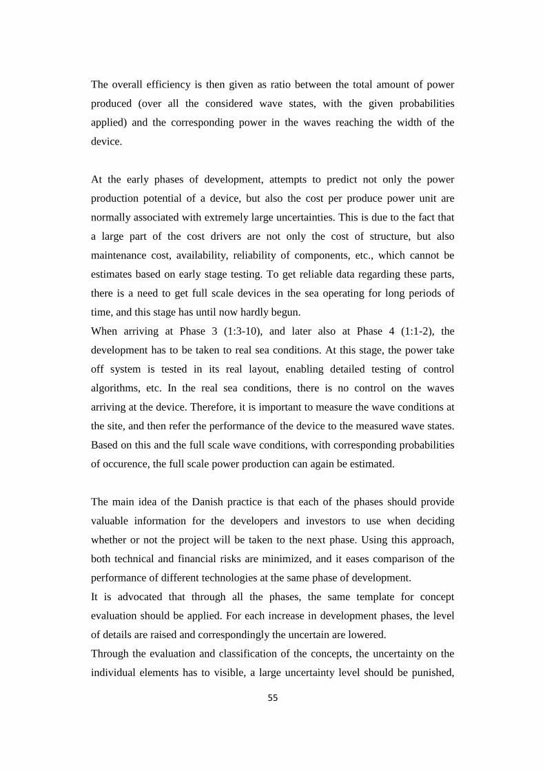
Figure 7.4: Comparison between the trend of the Irregular Italian Sea
and the trend of the Irregular Danish Sea…………………… 122
Figure 7.5: Danish efficiency trend for the Rolling Cylinder device……. 122
Figure 7.6: Danish efficiency trend and Italian efficiency trend………… 123
Figure 7.7: Wave Piston prototype in scale 1:30 in the laboratory of
Aalborg University………………………………………….. 126
Figure 7.8: Simulation of the device in the real sea……………………... 126
Figure 7.9: A plate of the Wave Piston………………………………….. 126
Figure 7.10: An hypothetical farm of Rolling Cylinder devices in the
Mediterranean Sea, Mazara del Vallo……………………….. 129
Figure 7.11: 3D-Rendering of the Rolling Cylinder device in the real sea 129
Figure 7.12: An hypothetical farm of Wave Piston devices in the
Mediterranean Sea, Mazara del Vallo……………………….. 130
Figure 7.13: 3D-Rendering of the Rolling Cylinder device in the real sea 131

8
TABLE INDEX
Table 2.1: Classification of Water Waves……………………………….. 20
Table 3.1: Scale Froude………………………………………………….. 52
Table 3.2: Standardized wave state describing energy in the Danish seas 53
Table 3.3: Equivalent periodic waves for tuning of power take off……... 54
Table 4.1: Planned tests in regular waves………………………………... 66
Table 4.2: Planned tests in irregular waves……………………………… 67
Table 4.3: Standardized wave states describing the Danish seas………... 68
Table 4.4: Scale Froude………………………………………………….. 68
Table 4.5: Wave height and wave period for regular and irregular waves
in scale 1:25…………………………………………………... 68
Table 5.1: Optimum Load and Efficiency for each value of fin’s
thickness and for different wave states……………………….. 78
Table 5.2: Optimum Load and Efficiency for different number of fins set
mounted on the model and for different wave states…………. 83
Table 5.3: Optimum Load and Efficiency for different number of fins
par set and for different wave states………………………….. 88
Table 5.4: Summarize of the performance of the Rolling Cylinder in
regular waves and full scale…………………………………... 93
Table 5.5: Summary of the performance of the Rolling Cylinder wave
energy converter in regular waves and full scale…………….. 94

9
Table 5.6: Summarize of the performance of the Rolling Cylinder in
irregular waves and full scale………………………………… 97
Table 5.7: Summary of the performance of the Rolling Cylinder wave
energy converter in irregular waves and full scale…………… 98
Table 7.1: Wave State describing Mazara del Vallo Sea………………… 120
Table 7.2: Wave State describing the Danish Sea……………………….. 120
Table 7.3: Wave State describing the Italian Sea in Mazara del Vallo….. 121
Table 7.4: Efficiency for the Italian Sea…………………………………. 123
Table 7.5: Summarize of the performance of the Rolling Cylinder in
irregular waves, in full scale and in an Italian installation 124
Table 7.6: Summary of the performance of the Rolling Cylinder wave
energy converter in irregular waves, in full scale and in an
Italian installation…………………………………………….. 125
Table 7.7: Summary of the performance of the Wave Piston wave
energy converter in an Italian installation. The value of the
power that can be converted from the waves into useful
mechanical power by the Wave Piston model is referred to
one plate of 15m of width . The device is subjected to
irregular wave…………………………………………………
127
Table 7.8: Summary of the performance of the Wave Piston wave
energy converter in irregular waves, in full scale and in an
Italian installation…………………………………………….. 127
Table 7.9: Comparison between the performance of the Rolling Cylinder
device and the Wave Piston device…………………………... 128
Table 7.10: Dimension in full scale of the Rolling Cylinder device and
Wave Piston device…………………………………………... 128

10
Table 7.11: Summary of the performance of an hypothetical farm of
Rolling Cylinder devices……………………………………... 130
Table 7.12: Summary of the performance of an hypothetical farm of
Wave Piston devices………………………………………….. 131
Table 8.1: Design optimization under regular waves……………………. 133
Table 8.2: Efficiency of the device under irregular waves………………. 134
Table 8.3: Summary of the performance of the Rolling Cylinder wave
energy converter under irregular waves, in full scale and in an
Italian installation, Mazara del Vallo………………………… 135
Table 8.4: Summary of the performance of the Wave Piston wave
energy converter under irregular waves, in full scale and in an
Italian installation, Mazara del Vallo………………………… 135
Table 8.5: Summary of the performance of an hypothetical farm of
Rolling Cylinder devices……………………………………... 136
Table 8.6: Summary of the performance of an hypothetical farm of
Wave Piston devices………………………………………….. 136

11
1. Introduction
The world energy consumption will rise enormously over the next decades, and
also the energy consumption in the European Union will increase in the same
period. To satisfy this energy demand different European countries start to focus
on generating electricity from renewable sources that are the only opportunity to
supply electricity and overcome negative aspects connected with traditional
methods of energy production. Being constantly reminded the seriously
environmental problems caused by traditional methods, the dramatic increase in
oil prices in 1973, the global attention to climate change and the rising level of
CO2, the governments of the Member States have seen the urgent need for
pollution-free power generation. In the dynamic evolution of the renewable
energy industry a wave energy industry is emerging. Although the technology is
relatively new, and currently not economically competitive with more mature
technologies such as wind energy, the interest from government and industry is
steadily increasing. An important feature of sea waves is their high energy
density, which is the highest among renewable energy sources [1].
Oceans waves are a huge, largely untapped energy resource, and the potential for
extracting energy from waves in considerable. Research in this area is driven by
the need to meet renewable energy targets, but is relatively immature compared to
other renewable energy technologies.

12

13
2. The wave energy resource
The sea is a huge water tank of energy of particularly high density, the highest
among the renewable. The utilization of this energy could cover a significant part
of the energy demand in Europe, and, moreover, it could make a substantial
contribution to a wide range of the objectives of environmental, social and
economic policies of the European Union [1].
The possibility of converting wave energy into usable energy has inspired
numerous inventors: more than thousand patents had been registered by 1980 [9]
and the number has increased markedly since then. The earliest such patent was
filed in France in 1799 by a father and a son named Girard [10].
In Europe intensive research and development study of wave energy conversion
began, however, after the dramatic increase in oil prices in 1973. Different
European countries with exploitable wave power resources considered wave
energy as a possible sources of power supply and introduced support measures
and related programs for wave energy. Several research programs with
government and private support started thenceforth, mainly in the United
Kingdom, Portugal, Ireland, Norway, Sweden and Denmark, aiming at developing
industrially exploitable wave power conversion technologies in the medium and
long term.
The efforts in research and development in wave energy conversion have gained
the support of the European Commission, which has, since 1986, been observing
the evolution in the wave energy field.
Starting in 1993, the Commission supported a series of international conferences
in wave energy, which significantly contributed to the simulation and
coordination of the activities carried out throughout Europe within universities,
national research centres and industry.
In the last 25 years wave energy has gone through a cyclic process of phases of
enthusiasm, disappointment and reconsideration. However, the persistent efforts
in R&D, and the experience accumulated during the past years, have constantly
improved the performance of wave power techniques and have led today to
bringing wave energy closer to commercial exploitation than ever before.

14
Different schemes have proven their applicability on a large scale, under hard
operational conditions, and a number of commercial plants are currently being
built in Europe, Australia, Israel and elsewhere. Other devices are in the final
stage of their R&D phase with certain prospects for successful implementation.
Nevertheless, extensive R&D work is continuously required, at both fundamental
and application level, in order to improve their steadily the performance of the
particular technologies and to establish their competitiveness in the global energy
market.
Figure 2.1: Wave power density around the world. The wave power density is very variable
around the world and its highest values are detected in the Oceans between the latitudes of
30° and 60° on both hemispheres

15
2.1 General aspects of wave energy
The wave energy is very much suited for countries with vast coast line and high
waves approaching the shore [12]. Waves are produced indirectly. The waves are
produced by sun by the following processes.
The total power of solar radiation incident on Earth atmosphere is tremendous.
When heated by sun, water evaporates, reducing the onset pressure. When there is
pressure difference, wind flows along the surface. The large movement of air
masses, vapour and water volumes creates the wind wave. Thus the main primary
energy source for all processes near the earth surface is the sun.
The movements of the sea surface, or known as sea waves is also caused by
external effects such as earthquakes, marine vehicles or attraction of gravity of the
moon and sun. Sea waves due to the wind are more continuously compared to sea
waves formed by other effects and therefore, they are considered primarily in
obtaining energy. Wave energy potential, as it is found in nature, is called natural
potential.
Technical potential is the transformed form of the natural potential to usable
energy by technological systems. The economic potential is the economically
defined amount when compared to the other energy sources [13].
In the past numerous researches [14-15] have been undertaken to quantify the
amount of wave power available at a particular location based on the values of
significant wave height (Hs), peak wave period (Tp) or energy wave period (Te).
All these studies examined the combined effect of Hs, Tp or Te on the power
estimation with a general aim to provide joint scatter plots.
The wave energy level is usually expressed as power per unit length (along the
wave crest or along the shoreline direction); typical values for “good” offshore
locations (annual average) range between 20 and 70 kW/m and occur mostly in
moderate to high latitudes. Seasonal variations are in general considerably larger
in the northern than in the southern hemisphere [16], which makes the southern
coasts of South America, Africa and Australia particularly attractive for wave
energy exploitation.
As a mathematical illustration of wave-energy extraction, we shall for simplicity
we consider wave power. The wave power estimation using the wave data will

16
give an account of the distribution of wave energy in space and time. Since the
last few decades, the hydrodynamics of ocean waves have been thoroughly
studied and now it is possible to determine the energy content of the sea with the
help of large amount of wave data collected. The power in wave can be expressed
by the formula [17]
P = 0.55 Hs2
T , kW/m of crest length (2.1.1)
where Hs, is the significant wave height in meter and T, is wave energy period in
seconds.
Waves are a very efficient way to transport energy: once created, waves can travel
thousands of kilometers with little energy loss . The size of a wave is determined
by three factors: wind speed, duration and the fetch, the distance over which the
wind blows transferring energy to the water.
Nearer the coastline the average energy intensity of a wave decreases due to
interaction with the seabed. Energy dissipation in near shore areas can be
compensated for by natural phenomena such as refraction or reflection, leading to
energy concentration (‘hot spots’).

17
2.2 Marine Energy and Wave Energy
It is essential to have an adequate knowledge of wave energy, to study the
conversion of wave energy to electricity. Waves on the surface of the ocean are
primarily generated by winds and are a fundamental feature of coastal regions of
the world. Knowledge of these waves, the forces they generate and estimates of
wave conditions are needed in almost all coastal engineering studies. In looking
the sea surface, it is typically irregular and three-dimensional (3-D). The sea
surface changes in time, and thus, it is unsteady. At this time, this complex, time-
varying 3-D surface cannot be adequately described in its full complexity; neither
can the velocities, pressures, and accelerations of the underlying water required
for engineering calculations. In order to arrive at estimates of the required
parameters, a number of simplifying assumptions must be made to make the
problems tractable, reliable and helpful through comparison to experiments and
observations. Some of the assumptions and approximations that are made to
describe the 3-D, time-dependent complex sea surface in a simpler fashion for
engineering works may be unrealistic, but necessary for mathematical reasons.
Wave theories are approximations to reality. They may describe some phenomena
well under certain conditions that satisfy the assumptions made in their derivation.
They may fail to describe other phenomena that violate those assumptions. In
adopting a theory, care must be taken to ensure that the wave phenomena of
interest is described reasonably well by theory adopted, since shore protection
design depends on the ability to predict wave surface profiles and water motion,
and on the accuracy of such predictions.
Regular waves and linear wave theory
The most elementary wave theory is the small-amplitude or linear wave theory.
This theory developed by Airy (1845), is easy to apply, and gives a reasonable
approximation of wave characteristic for a wide range of parameters.
Many engineer problems can be handled with ease and reasonable accuracy by
this theory. For convenience, prediction method in coastal engineering generally
have been based on simple waves. For some situations, simple theories provide
acceptable estimates of wave conditions.

18
The linear theory represents pure oscillatory waves. Waves defined by finite-
amplitude wave theories are not pure oscillatory waves but still periodic since the
fluid is moved in the direction of wave advance by each successive wave. This
motion is termed mass transport of the waves. Other assumptions made in
developing the linear wave theory are:
- the fluid is homogeneous and incompressible; therefore the density ρ is a
constant;
- surface tension can be neglected;
- Coriolis effect due to earth’s rotation can be neglected;
- pressure at the free surface is uniform and constant;
- the fluid is ideal or inviscid (lacks viscosity);
- the particular wave being considered does not interact with any other
water motions. The flow is irrotational so that water particles do not rotate;
- the bed is a horizontal, fixed, impermeable boundary, which implies that
the vertical velocity at the bed is zero;
- the wave amplitude is small and the waveform is invariant in time and
space;
- waves are plane or long-crested (two-dimensional).
A progressive wave may be represented by the variables x (spatial) and t
(temporal) or by their combination (phase), defined as Φ = kx - t. A simple,
periodic wave of permanent form propagating over a horizontal bottom may be
completely characterized by the wave height H and wavelength L and water depth
d. The highest point of the wave is the crest and the lowest point is the trough. For
linear or small-amplitude waves, the height of the crest above the still-water level
(SWL) and the distance of the trough below the SWL are each equal to the wave
amplitude a. Therefore a = H/2, where H = the wave height. The time interval
between the passage of two successive wave crests or trough at a given point is
the wave period T. The wavelength L is the horizontal distance between two
identical points on two successive wave crests or two successive wave troughs
and denotes the displacement of the water surface relative to the SWL and is a
function of x and t. Other wave parameters include = 2π/ T the angular or

19
radian frequency, the wave number k = 2π/L, the phase velocity or wave celerity c
= L/T = /k, the wave steepness = H/L. These are the most common parameters
encountered in coastal practice.
An expression relating wave celerity (c) to wave length (L) and water depth (d) is
given by:
The values 2π/L and 2π/T are called the wave number k and the wave angular
frequency respectively. From the equation c = L/T and from the Eq. 2.2.1 , an
expression for wavelength as a function of depth and wave period may be
obtained as:
Figure 2.2: Main parameters of wave

20
Waves may also be classified by the water depth in which they travel. The
following classification are made according to the magnitude of d/L and the
resulting limiting values taken by the function tanh (2πd/L). Note that as the
argument of the hyperbolic tangent kd = 2πd/L gets large, the tanh (kd)
approaches 1, and for small values of kd, tanh (kd) kd.
Classification d/L kd tanh (kd)
Deep water 1/2 to π to = 1
Transitional 1/20 to 1/2 π/10 to π tanh (kd)
Shallow water 0 to 1/20 0 to π/10 = kd
Table 2.1: Classification of Water Waves
In deep water, tanh (kd) approaches unity, Eq.2.2.1 reduce to:
and:
When the relative water depth (d/L) becomes shallow, Eq. 2.2.1 can be simplified
to:
Thus, when a wave travels in shallow water, wave celerity depends only on water
depth.

21
In summary, as a wind wave passes from deep water to the beach its speed and
length are first only a function of its period; then as the depth becomes shallower
relative to its length, the length and speed are dependent upon both depth and
period; and finally the waves reaches a point where its length and speed are
dependent only on depth ( and not frequency).
The equation describing the free surface as a function of time t and horizontal
distance x for a simple sinusoidal wave can be shown to be:
where:
- = the elevation of the water surface relative to the SWL;
- H/2 = one-half the wave height equal to the wave amplitude a.
This expression represents a periodic, sinusoidal, progressive wave travelling in
the positive x-direction.
Figure 2.2.2, a sketch of the local fluid motion, indicates that the fluid under the
crest moves in the direction of wave propagation and returns during passage of the
trough. Linear theory does not predict any net mass transport; hence, the sketch
shows only an oscillatory fluid motion.

22
Figure 2.3: Local fluid velocities and accelerations
Another important aspect of linear wave theory deals with the displacement of
individual water particles within the wave. Water particles generally move in
elliptical paths in shallow or transitional depth water and in circular paths in deep
water (Figure 2.2.3).
Figure 2.4: Elliptical paths in shallow or transitional depth water and in circular paths in deep water
It is desirable to know how fast wave energy is moving. One way to determine
this is to look at the speed of wave groups that represents propagation of wave

23
energy in space and time. The speed a group of waves or a wave train travels is
generally not identical to the speed with which individual waves within the group
travel. The group speed is termed the group velocity Cg; the individual wave
speed is the phase velocity or wave celerity given by Eq. 2.2.1. For waves
propagating in deep or transitional water with gravity as the primary restoring
force, the group velocity will be less than the phase velocity.
In deep water the group velocity is one-half the phase velocity:
In shallow water the group and phase velocities are equal:
Thus, in shallow water, because wave celerity is determined by the depth, all
component waves in a wave train will travel at the same speed precluding the
alternate reinforcing and canceling of components. In deep and transitional water,
wave celerity depends on wavelength; hence, slightly longer waves travel slightly
faster and produce the small phase differences resulting in wave groups.
The total energy of a wave system is the sum of its kinetic energy and its potential
energy.
The kinetic energy is that part of the total energy due to water particle velocities
associated with wave motion. The kinetic energy per unit length of wave crest for
a wave defined with the linear theory can be found from:

24
Where:
- ρ = density wave power [kg/m3];
- u = fluid velocity in x-direction [m/s];
- w = fluid velocity in z-direction [m/s].
The Eq. 2.2.9 , upon integrations, gives:
Potential energy is that part of the energy resulting from part of the fluid mass
being above the trough: the wave crest. The potential energy per unit length of
wave crest for a linear wave is given by:
which, upon integrations, gives:
According to the Airy theory, if the potential energy is determined relative to
SWL, and all waves are propagated in the same direction, potential and kinetic
energy components are equal, and the total wave energy in one wavelength per
unit crest width is given by:

25
where subscripts k and p refer to kinetic and potential energies. Total average
wave energy per unit surface area, termed the specific energy or energy density, is
given by:
Wave energy flux is the rate at which energy is transmitted in the direction of
wave propagation across a vertical plan perpendicular to the direction of wave
advance and extending down the entire depth.
Assuming linear theory holds, the average energy flux per unit wave crest width
transmitted across a vertical plane perpendicular to the direction of wave advance
is
Where:
- p = gauge pressure;
- t = start time;
- r = end time.

26
Figure 2.5: The kinetic and potential energy of the wave energy
The Eq. 2.2.15 , upon integrations, gives:
where is frequently called wave power.
For deep and shallow water, the Eq. 2.2.16 becomes:
The wave energy flux (P) is also called wave power. The wave theory indicates
that wave power is dependent on three basic wave parameters: wave height, wave
period and water depth.
Nevertheless the real sea is composed by an irregular wave situations, in first
approximation the following formula can be used to estimate the energy flux of an
irregular wave in deep water conditions:

27
Where:
- P= wave energy flux per unit wave crest length [kW/m];
- ρ = mass density of the sea water 1030 [kg/m3];
- g = acceleration by gravity 9.81 [m/s2];
- T= wave period [s];
- β = is a coefficient may be 64 for irregular waves or 32 for regular waves.
Irregular waves
In the first part of this chapter, waves on the sea surface were assumed to be
nearly sinusoidal with constant height, period and direction. Visual observation of
the sea surface and measurements indicate that the sea surface is composed of
waves of varying heights and periods moving in differing directions. Once we
recognize the fundamental variability of the sea surface, it becomes necessary to
treat the characteristics of the sea surface in statistical terms. This complicates the
analysis but more realistically describes the sea surface. The term irregular waves
will be used to denote natural sea states in which the wave characteristics are
expected to have a statistical variability in contrast to monochromatic waves,
where the properties may be assumed constant. Monochromatic waves may be
generated in the laboratory but are rare in nature.
Two approaches exist for treating irregular waves: spectral methods and wave-by-
wave (wave train) analysis.
Unlike the wave train or wave-by-wave analysis, the spectral analysis method
determines the distribution of wave energy and average statistics for each wave
frequency by converting time series of the wave record into a wave spectrum.
This is essentially a transformation from time-domain to the frequency domain,
and is accomplished most conveniently using a mathematical tool known as the
Fast Fourier Transform (FFT) technique.
The wave energy spectral density E(f) or simply the wave spectrum may be
obtained directly from a continuous time series of the surface η(t) with the aid of

28
the Fourier analysis. Using a Fourier analysis, the wave profile time trace can be
written as an infinite sum of sinusoids of amplitude An, frequency ωn , and relative
phase εn, that is:
Physically, m0 represents the area under the curve of E(f) and the area under the
spectral density represents the variance of a random signal.
The above definition of the variance of a random signal can be use to provide a
definition of the significant wave height. For Rayleigh distributed wave heights,
Hs may be approximated by:

29
Figure 2.6 : A spectrum [28]
There are many forms of wave energy spectra used in practice, which are based
on one or more parameters such as wind speed, significant wave height, wave
period, shape factors, etc.
The most common spectrum is the JONSWAP spectrum. This is a five-parameter
spectrum, although three of these parameters are usually held constant.

30
Characteristic wave height for an irregular sea state may be defined in several
ways. These include the mean height, the root-mean-square height, and the
significant height.
The root-mean-square height is a regular wave height parameter containing the
same wave energy density as the measured irregular Tp wave record and can be
determined as:
Significant wave height Hs can be estimated from a wave-by-wave analysis in
which case it is denoted H1/3 and is the average height of the third-highest waves
in a record of time period but more often is estimated from the variance of the
record or the integral of the variance in the spectrum in which case it is denoted
Hm0.
The characteristic period could be the mean period, energy period (Te) or peak
period (Tp).
Similarly to the equivalent wave height parameter, HRMS, a regular wave period
parameter is required with equivalent energy density to that of the irregular wave
record. This regular wave period is called is called the energy period (Te) and is
determined by integrating the wave energy density spectrum.
The inverse of the frequency in the recorded wave energy density spectrum at
which maximum energy density occurs is known as the peak period (Tp) of the
record. This is a very important parameter frequently used in coastal engineering
applications [28].

31
2.3 Advantages and disadvantages of wave energy
Using waves as a source of renewable energy offers both advantages and
disadvantages over other methods of energy generation.
The most important difficulties facing wave power developments are:
Irregularity in wave amplitude, phase and direction; it is difficult to obtain
maximum efficiency of a device over the entire range of excitation
frequencies.
The structural loading in the event of extreme weather conditions, such as
hurricanes, may be as high as 100 times the average loading.
The wave power’s variability in several time-scales: from wave to wave,
with sea state, and from month to month.
It becomes apparent, that the design of a wave energy converter has to be highly
sophisticated to be operationally efficient and reliable on the one hand, and
economically feasible on the other. As with all renewable energy sources, the
available resource and variability at the installation site has to be determinate first.
The main wave energy barriers result from the energy carrier itself, the sea. As
stated previously, the peak-to-average load ratio in the sea is very high, and
difficult to predict. It is, for example, difficult to define accurately the 50-years
return period wave for a particular site, when the systematic, in situ recording of
wave properties started just a few years ago.
The result is either underestimation or overestimation of the design loads for a
device. In the first case the total or partial destruction of the facilities is to be
expected. In the second case, the high construction costs induce high power
generation costs, thus making the technology uncompetitive. These constraints,
together with misinformation and lack of understanding of wave technology by
the industry, government and public, have often slowed down wave energy
development [2].

32
On the other hand, the advantage of wave energy are obvious:
Sea waves offer the highest energy density among renewable energy
sources [1].
Limited negative environmental impacts. The demand on land use is
negligible and wave power is considered a clean source of renewable
energy that not involving large CO2 emissions. In general, offshore
devices have the lowest potential impact.
The development of wave energy is sustainable, as it combines crucial
economic, environmental, ethical and social factors.
Natural seasonal variability of wave energy, which follows the electricity
demand in temperate climates.
Waves can travel large distances with little energy loss. Storms on the
western side of Atlantic Ocean will travel to the western coast of Europe,
supported by prevailing westerly winds.
Wave power devices can generate power up to 90 per cent of the time,
compared to 20-30 per cent for wind and solar power devices [3,4].
To realize the benefits listed above, there are a number of technical challenges
that need to be overcome to increase the performance and hence the commercial
competitiveness of wave power devices in the global energy market.
A significant challenge is the conversion of the slow, random, and high-force
oscillatory motion into useful motion to drive a generator with output quality
acceptable to the utility network. As waves vary in height and period, their
respective power levels vary accordingly. While gross average power levels can
be predicted in advance, this variable input has to be converted into smooth
electrical output and hence usually necessitates some type of energy storage
system, or other means of compensation such ad an array of devices.
Additionally, in offshore locations, wave direction is highly variable, and so wave
devices have to align themselves accordingly on compliant moorings, or be
symmetrical, in order to capture the energy of the wave. The directions of waves
near the shore can be largely determined in advance owing to the natural
phenomena of refraction and reflection.

33
The challenge of efficiently capturing this irregular motion also has an impact on
the design of the device. To operate efficiently, the device and corresponding
systems have to be rated for the most common wave power levels. However, the
device also has to withstand extreme wave conditions that occur very rarely, but
could have power levels in excess of 2000 kW/m.
Not only does this pose difficult structural engineering challenges as the normal
output of the device are produced by the most commonly occurring waves, yet the
capital cost of the device construction is driven by a need to withstand the high
power level of the extreme, yet infrequent, waves [11]. There are also design
challenges in order to mitigate the highly corrosive environment of devices
operating at the water surface [1].
Lastly, the research focus is diverse. To date, the focus of the wave energy
developers and a considerable amount of the published academic work has been
primarily on sea performance and survival, as well as the design and concept of
the primary wave interface. However, the methods of using the motion of the
primary interface to produce electricity are diverse. More detailed evaluation of
the complete systems is necessary if optimized, robust yet efficient system are to
be developed.

34
2.4 Wave Energy in Europe
Research and development on wave energy is underway in several European
countries. The engagement in wave energy utilization depends strongly on the
available wave energy resource. In countries with high resources, wave power
could cover a significant part of the energy demand in the country and even
become a primary source of energy. Countries with moderate, though feasible
resources, could utilize wave energy supplementary to other available renewable
and/or conventional sources of energy.
Denmark, Ireland, Norway, Portugal, Sweden and the United Kingdom
considered wave power a long time ago as a feasible energy source. These
countries have significant wave power resources and have been actively engaged
in wave energy utilization under governmental support for many years [1].
Figure 2.7 : Wave power density in Europe. In Europe the West coasts of the U.K. and Ireland
along with Norway and Portugal receive the highest power densities

35
Denmark
Denmark lies in a sheltered area in the southern part of the North Sea, however,
in the North-western regions the wave energy resource is relatively favourable for
potential developments. The annual wave energy resource of Denmark has been
estimated to be about 30 TWh with an annual wave power between 7 and 24
kW/m coming from a westerly direction. The Danish Wave Energy Programme
started in 1996 with Energy 21. The objective is to promote wave energy
technology following the successful Danish experience of wind energy.
Ireland
Ireland has considerable potential for generating electricity from wave power.
According to Lewis the total incident wave energy is around 187,5 TWh.
At present, a partnership of the Hydraulic & Maritime Research Centre,
University College Cork, Irish Hydrodata Ltd, Ove Arup & Partners Ltd, the
Department of Mechanical and Aeronautical Engineering, University of Limerick
and the Marine Institute are finalizing a Strategic Study on Wave Energy in
Ireland. The objective of the study is to provide a scaled selection of wave energy
sites and to investigate a wave climate prediction methodology.
Norway
Norway has a long coastline facing the Eastern Atlantic with prevailing west
winds and high wave energy resources of the order of 400 TWh/year. Even
though there is high wave energy availability, due to the economics and the
uncertainties of the available technology, the conclusion of Energy and Electricity
Balance towards 2020 are that 0,5 MWh will be the wave energy contribution to
the Norwegian electricity supply, mainly from small-scale developments.
All of Norway’s electricity supply has traditionally been renewable hydropower,
but the increased electricity demand of recent years has not been met by an equal
increase in power plants, due to public opposition to large hydropower
developments.
The government is promoting land based wind and biomass, with particular focus
on hydrogen as an energy carrier and gas fuel cell pilot projects. The

36
environmental concern of high CO2 emission from power generation for oil and
gas offshore installations could create the basis for a potential wave energy
market.
Norway started its involvement in wave energy in 1973 in the Norwegian
University of Science and Technology (NTNU). In the 1980s two shoreline wave
converters were developed, the Multi-Resonant Oscillating Water Column, OWC
and the Tapered Channel, Tapchan but the plants were seriously damaged during
storms in 1988 and 1991. Anyway there are plans for re-opening the Tapchan
plant.
Portugal
Portugal is characterised by an annual wave power of between 30 and 40 kW/m.
The highest wave power is found off the northwestern coast of Portugal and in the
archipelago of the Azores. It has been estimated that the overall resource of wave
energy on continental Portugal is about 10 GW mean, and half of it can be
potentially exploited.
The Portuguese government supports wave energy, as other renewable energy
technologies, through different financial mechanisms. Since 1986, Portugal has
been successfully involved in the planning and construction of the shoreline wave
energy converter Oscillating Water Column in Pico of the Azores.
Sweden
Sweden has a few good areas for utilising wave energy. The north parts of the
west coast facing the North Sea and the Baltic Sea around the islands of Oland
and Gotland. The technically available resource is approx. 5–10 TWh per annum.
This is to be compared with the annual electricity demand of 150 TWh in Sweden.
Wave Energy research started in Sweden in 1976. In 1980 the first full scale point
absorber buoy in the world was installed outside Goteborg. Another large project
was the Hose-Pump project. It was also full scale tested at sea, 1983-1986.

37
United Kingdom
The United Kingdom is located at the eastern end of the long fetch of the Atlantic
Ocean with the prevailing wind direction from the west, and it is surrounded by
stormy waters. The available wave energy resource is estimated to be 120 GW.
Wave energy started in the UK at the University of Edinburgh when the oil crisis
in 1973 hit the whole world. In 1974, S. Salter published his initial research work
on wave power and the research on the offshore wave energy converter, the Salter
Ducks, was started.
In the meantime at least another ten wave energy projects were initiated in the
UK. Furthermore, the success of the initial Limpet OWC project and its full
decommissioning in 1999 has created the basis for including three wave energy
projects in the third Scottish Renewable Obligation.
Other European Countries
Due to political reasons, mainly the focalisation to other energy sources, or lack of
feasible resources, wave energy conversion has not undergone significant
development in Belgium, Finland, France, Germany, Greece, Italy, the
Netherlands and Spain in the past years.
Belgium, Germany and the Netherlands are characterized by a relatively limited
length of coastline, shallow coastal water and high offshore traffic density. All
these factors militate against significant interest in wave energy development.
France has a long coastline on the Atlantic and the Mediterranean Seas. Although
a number of successful wave energy project were operated in France during the
early part of the last century, wave energy conversion has not undergone
significant development in the recent past.
Greece has a coastline of over 16000 km ones in the Aegean and Ionian Seas.
Wave power plants are particularly suitable for delivering electricity to the large
number of islands, which are mainly supplied by diesel stations. The high cost of
electricity on the islands will make wave energy competitive against conventional
power producers; however, wind energy has already proven its feasibility in this
region, and it is heavily supported by the government and private investors.

38
Italy has a long coastline in relation to its land area and would appear suitable for
utilisation of ocean energy. Wave studies around the coastline, however, show
that, in general, the wave power annual average is less than 5 kW/m. There are a
number of offshore islands and specific locations, such as Sicily or Sardinia,
where the mean wave energy is higher, up to approx. 10 kW/m.

39
3. Wave energy converters
In contrast to other renewable energy resource utilization, there is a wide variety
of wave energy technologies, resulting from the different ways in which energy
can be absorbed from the wave, and also depending on the water depth and on the
location. This large number of concepts for wave energy converters (WECs) is
generally categorized by location, type and working principle.
3.1 Location
Shoreline devices: they are fixed to the shoreline itself and have the advantage of
being close to the utility network. Then they also have the advantage of being
easy to maintain and to install. In addition they do not require deep-water
moorings or long lengths of underwater electrical cable and as waves are
attenuated as they travel through shallow water they have a reduced likelihood of
being damaged in extreme conditions. However the wave power in the shallow
water is lower and by nature of their location they have to satisfy specific
requirements for shoreline geometry and preservation of coastal scenery.
An example of shoreline device is the SSG (Sea Slot-cone Generator), a wave
energy converter of the overtopping type: the overtopping water of incoming
waves is stored in different basins depending on the wave height. The structure
consists of a number of reservoirs one on the top of each other above the mean
water level in which the water of incoming waves is stored temporary. In each
reservoir, expressively designed low head hydroturbines are converting the
potential energy of the stored water into power. A key to success for the SSG is
the low cost of the structure and its robustness.
Turbines play an important and delicate role on the power takeoff of the device.
They must work with very low head values (water levels in the reservoirs) and
wide variations in a marine aggressive environment. The main strength of the
device consists on robustness, low cost and the possibility of being incorporated
in breakwaters (layout of different modules installed side by side) or other coastal
structures allowing sharing of costs and improving their performance while

40
reducing reflection due to efficient absorption of energy. Even though, an offshore
solution of the concept could be investigated to reach more energetic sea climates
[26].
Figure 3.1: Lateral section of a three-levels SSG device [26]
Nearshore devices: they are for moderate water depths (i.e < 20 m). Devices in
this location are often attached to the seabed, which gives a suitable stationary
base against an oscillating body can work [5]. They have the same disadvantage
of the shoreline devices, because the waves have reduced power in the shallow
water.
An example of shoreline device is an oscillating water column device (OWC)
called the OSPREY (Ocean Swell Powered Renewable EnergY), which
incorporates a wind turbine.
The steel design is shown in Figure 3.2. It comprises a 20 m wide rectangular
collector chamber in the centre, with hollow steel ballast tanks fixed to either side.
These tanks face into the principal wave direction and focus the waves towards
the opening in the collector chamber. The air flow from this chamber passes
through two vertical stacks mounted on the chamber. Each of these contains two,
contra-rotating Wells’ turbines, each of which is attached to a 500 kW generator.

41
A control module is also mounted on top of the collector chamber, containing the
power control equipment, transmission system, crew quarters, etc. Behind the
collector chamber and power module is a conning tower on which can be mounted
a “marinised” wind turbine.
The whole device is designed for installation in a water depth of approximately 14
m and weighs approximately 750 t.
Figure 3.2: The steel OSPREY Design
Offshore devices: they are generally in deep water ( > 40m ). The advantage of
locating a device in deep water is that they can obtain a big amount of energy
because of the higher wave power in deep water. On the other hand these devices
are more difficult to install and to maintain and they need to survive the more
extreme conditions. Also the cost of construction is more expensive. Offshore

42
devices are basically oscillating bodies, either floating or (more rarely) fully
submerged and in general more complex compared with the nearshore devices.
This, together with additional problems associated with mooring, access for
maintenance and the need of long underwater electrical cables, has blindered their
development, and only recently some systems have reached, or come close to, the
full-scale demonstration stage [2].
An example of offshore devices is the “Mighty Wale”, which is a floating wave
energy device based on the oscillating water column (OWC) principle. It converts
wave energy into electric energy, and produces a relatively calm sea behind. This
calm area can be utilized for varied applications such as fish farming. Jamsted
completed the construction of the prototype device “Mighty Whale” by May 1998
for open sea tests to investigate practical use of wave energy. Following
construction, the prototype was towed to the test location near the mouth of
Gokasho Bay in Mie Prefecture. The open sea tests were begun in September
1998, after final positioning and mooring operations were completed.
The “Mighty Whale” is a steel floating structure with the appearance of a whale
which has an air chamber section for adsorbing the wave power energy at the
front (windward), buoyancy tanks and a stabilizer slope for reducing pitching
motions in the waves. Each air chamber has an opening at the top where and air
turbine power generator is installed. The under water front wall of each air
chamber is open to allow entry of the wave. When a wave enters the air chamber,
the water surface inside it moves up and down, producing an oscillating airflow,
which passes through the opening at the top of the air chamber. This airflow is
used to drive the air turbine and generator. This is a wave power energy converter
of oscillating water column type. The air turbine mounted on the “Mighty Whale”
are Wells turbines featuring stable rotation of the same direction in an oscillating
airflow [27].

43
Figure 3.3: The prototype [27]
3.2 Type
Attenuator: these devices are arranged parallel to the predominant wave direction.
An example of an attenuator WEC is the Pelamis.
The Pelamis is a floating device comprised of cylindrical hollow steel segments
(diameter of 3,5 m) connected to each other by two degree-of-freedom hinged
joints. Each hinged joint is similar to a universal joint, with the central unit of
each joint containing the complete power conversion system. The wave-induced
motion of these joints is resisted by four hydraulic cylinders that accommodate
both horizontal and vertical motion. These cylinders act as pumps, which drive
fluid through a hydraulic motor, which in turn drives an electrical generator.
Accumulators are used in the circuit to decouple the primary circuit (the pumps)
with the secondary circuit (the motor), and aid in regulating the flow of fluid to
produce a more constant generation. The hydraulic power take off (PTO) system
uses only commercially available components. Each Pelamis is 120 m long, and
contains three power modules, each rated at 250kW. It is designed to operate in

44
water depths of 50 m. The shape and loose mooring of Pelamis lets it orient itself
to the predominant wave direction, and its length is such that it automatically
“detunes” from the longer-wavelenght high-power waves, enhancing its
survivability in storms [9]. A wave farm using Pelamis was recently installed 3
miles from Portugal’s northern coast, near Pòvoa do Vorzina. This followed full-
scale prototype testing at EMEC facility in Orkney [10]. The wave farm initially
uses three Pelamis machines developing a total power of 2,25 MW.
Point absorber : these devices have a small dimensions in comparison with the
incident wavelength, they are able to capture energy from a wave front greater
than the physical dimension of the absorber and because of their small size wave
direction is not important for these device and it is able to capture energy from
waves arriving from any directions. They can be floating structures that moves up
and down on the surface of the water or submerged below the surface. An
example of point absorber is Ocean Power Technology’s Powerbuoy. The
Powerbuoy is a floating point absorber buoy, based on the relative movement
between the inner and outer parts that constitute the device. The outer part of the
buoy has a circular shape, it is floating near water’s surface and it moves with the
waves. The inner part of the buoy is a vertical pipe that contain a compressible
volume of air. As the crest of the wave passes over the device, the air is
Figure 3.4: Attenuator device: Pelamis wave farm

45
compressed and the inner part moves downwards. This motion is used to spin a
generator, and the electricity is transmitted to shore over a submerged
transmission line.
Terminator: the principal axis of these devices is perpendicular to the
predominant wave direction, they obstruct the transit for the waves and they catch
the wave energy. An example of a terminator-type WEC is the Salter’s Duck. This
device has a egg-shaped. Each incoming wave moves up and down the “duck”
and this motion compresses air through the Duck driving turbines which create
electricity.
Figure 3.5: Point absorber device: OPT Powerbuoy

46
3.3 Working principle
Oscillating water column (OWC) : an OWC consists of a partly submerged
concrete or steel chamber with an opening to the sea below the waterline and an
opening to the air via one or more air turbines. When the incoming waves impact
the device, the water is forced into the chamber, and the water level inside the
chamber rises and falls, compressing and expanding an air column and driving it
through the air turbine that drives an electrical generator. Since the air direction
reverses halfway through each wave, a method of rectifying the airflow is
required; although systems employing multiple turbines with one-way valves have
been used, the currently favored method involves the use of a “self-rectifying”
turbine that spins in only one direction regardless of the direction of airflow [6].
For this reason ,in this application is often used a low-pressure Wells turbine as it
rotates in only one direction irrespective of the flow direction, removing the need
to rectify the airflow [5]. Full sized OWC prototypes were built in Norway, Japan,
India, Portugal, UK. The largest of all, a nearshore bottomstanding plant was
destroyed by the sea shortly after having been towed and sunk into place near the
Scottish coast.
An example of OWC systems is the Limpet, a shoreline device installed on the
island of Islay, Western Scotland. This device has an inclined oscillating water
Figure 3.6: Terminator device: Salter's Duck

47
column and water depth at the entrance of the OWC is typically seven metres. The
design of the air chamber is important to maximize the capture of wave energy
and the turbines are carefully matched to the air chamber to maximize power
output.
Overtopping device: this device captures the water that is close to the wave crest
and introduce it, by over spilling, into a reservoir where it is stored at a level
higher than the average free-surface level of the surrounding sea. . The energy is
extracted by using the difference in water level between the reservoir and the sea
and the potential energy of the stored water is converted into useful energy
through more or less conventional low-head hydraulic turbines. Then the water is
allowed to return to the sea through turbines. Overtopping devices do possess an
advantage in that their turbine technology has already been in use in the
hydropower industry for a long time and is thus well understood [6].
An example of such a device is the Wave Dragon, an offshore converter
developed in Denmark. This device uses two large reflectors that stretch outwards
Figure 3.7: OWC: The Limpet

48
from the device and orient waves towards the central receiving part. The sea water
is collected in a raised reservoir from which water is released via a number of
low-head turbine. A 57 m-wide, 237 t prototype of the Wave Dragon has been
deployed in Nissum Bredning, Denmark, and has been tested for several years [2].
Wave activate body (WAB): in this device the waves activate the oscillatory
motions of parts of the device relative to the other parts of the device or of one
part relative to a fixed reference. Primarily heave, pitch and roll motions can be
identified as oscillating motions whereby the energy is extracted from the relative
motion of the bodies or from the motion of one body relative to its fixed reference
by using typically hydraulic systems to compress oil, which is then used to drive a
generator [8].
An example of WAB device is DEXA. Dexa is characterized by a simple
structure. There are two pontoons connected together in the middle point of the
device in order that each pontoon can rotate relative to the other.
Figure 3.8: Overtopping principle

49
3.4 Development for WEC tests and developments
Starting at the initial idea the development of a wave energy has to go through
different phases before the first prototypes can be placed in open sea. Usually this
development starts with theoretical analyses, then there are experiments in the
wave tank at a small and an intermediate scale before to deploy the first prototype
in the sea.
Now in Denmark there is a work that summarizes the best practice to put into
practice a wave energy device. This practice is constituted by four phases. The
main idea is that each phase has to give some specific information to the inventor
and his investors. Secondary the idea is not to use too many resources before
having an estimate on the potential.
The four phases used in Denmark are [7]:
Phase 1: Proof of concept. Rough estimates of energy production in five
specified wave states leading to an estimate of a yearly energy production.
Suggestions for further development of the device. Typical small
indicative laboratory tests followed by a 10 page report. Cost 10.000 €.
Phase 2: Design and feasibility study. Typically through detailed
laboratory tests in scale 1:50 to 1:20. Detailed Numerical calculations,
estimates on cost, feasibility studies, Power take-off (PTO) design, etc.
Typical intensive laboratory tests (optimizations) or intensive numerical
Figure 3.9: DEXA, an example of Wave Activate Body

50
modeling. This phase can consist of N (i.e. 10) detailed investigations
followed by 100 page reports. Cost 25.000-50.000 €.
Phase 3: Testing in real seas in scale 1:10 to 1:3. Normally Nissum
Bredning, a “small” benign piece of inner sea, a part of the Limfjord in the
northern part of Denmark , has been used for this purpose. Cost 0.5-5
million €.
Phase 4: Demonstration in half or full scale. Cost 5-20 million €.
Figure 3.10: Location of Nissum Bredning in Denmark
The main instrument used under phase 1 and phase 2 to assess the wave energy
devices is small scale testing in a hydraulic laboratory. These tests are performed
in order to gain knowledge on the devices before they actually are built and
deployed in the sea. The laboratory tests will give information on:

51
a. Loads on the device
b. Movements of the device
c. Run-up / overtopping of the device
d. Energy production
In phase 1 assessment, the test will give rough estimates (± 20%) on energy
production, and knowledge from the tests will help to estimate costs. In a Phase 2
assessment, the test will give more detailed estimates (± 5%) on the expected
energy production.
A phase 2 test could further include a parametric study making it possible to
optimize the device. By far the most frequently used model law in relation to
wave laboratory tests in Froudes Model Law, which requires:
- Inertia forces to dominate the physics. Friction forces must be negligible
relative to the inertia forces. Inertia forces are forces proportional to the
volume/mass of the device.
- The model must be geometrically similar to the full scale device.
The requirement of friction forces to be small relative to the inertia forces will
tipically lead to a maximum scale ratio in the order of 1:50 for device models to
be testes in wave laboratory. On the other hand, most power off systems cannot
within reason be scaled more than 1:10 at the most, mainly due to frictional
losses.
Wave basins are normally designed for hydraulic tests with marine constructions,
ships, or coastal structures. In order to keep costs down, such tests are
traditionally performed in scale 1:20 to scale 1:100. If a design wave height is 15
metres with a period of 12 seconds, a model test in scale 1:100 will be performed
with a wave height of 15 cm and a period of 1.2 seconds.
The wave energy sector often wants to perform tests in i.e. scale 1:10. For the
previous example, that would give a wave height equal to 1.5 metres with a period
of 3.8 seconds. Model tests with such large waves can be performed in a very few
laboratories around the world, and costs are enormous. Therefore model tests are

52
performed in i.e. scale 1:40, which leads to scale effects on the modeling of the
power take off.
Consequently, the power take off is modeled to perform in accordance with pre-
specified characteristics. This is not a serious problem because one of the
requirements to the outcome of the model tests often is a specification on the
loading of the power take off. One should always remember that the dimensions
of the power take off system cannot simply be scaled up. It is the performance
which can.
Transferring measured data to full scale values follows the Froudes Model Law:
Parameter Model Full Scale
Length 1 S
Area 1 S2
Volume 1 S3
Time 1 S0,5
Velocity 1 S0,5
Force 1 S3
Power 1 S3,5
Table 3.1: Scale Froude
Waves are by nature irregular, short crested, and non-linear. The question is: How
accurate is it necessary to model the sea.
The energy content in the seas around Denmark varies from location to location.
Excluding the very extremes, the Danish seas have areas with average energy
levels ranging from 5 to 22 kW/metre wave crest. Scatter diagrams exist for many
parts of the Danish seas. It is obvious that a detailed design/optimization must
take into account the actual waves existing on the proposed location for the wave
energy device, but in order to make some comparison possible for devices being
tested under phase 1 (and phase 2), devices are normally tested against 5 pre-
defined wave states describing energy content of the sea.

53
wave state Hs [m] Tz [s] Tp [s] Energy flux [kW/m] Prob. Occur. [%]
1 1.0 4.0 5.6 2.1 46.8
2 2.0 5.0 7.0 11.6 22.6
3 3.0 6.0 8.4 32.0 10.8
4 4.0 7.0 9.8 65.0 5.1
5 5.0 8.0 11.2 114.0 2.3
Table 3.2: Standardized wave state describing energy in the Danish seas
In phase 1, the sea is always modeled as linear irregular long crested waves using
JONSWAP spectra with a peak enhance factor equal to 3.3.
Hs is significant wave height as defined by International Association of Hydraulic
Engineering and Research, and Tz is average wave period based on zero-down
crossing analysis, and Tp is peak period of the wave spectrum.
For tests to assess the energy production, the minimum duration of the tests in
each irregular wave state is 500 waves.
A precise modeling of the power take off is important because of two reasons:
- The power production is responsible for all the income from the device.
- The load from the power take feeds back to the hydraulic performance of
the device.
Therefore, the load from the power take off on the system has to be controllable.
In a full scale wave energy device, the power take off system as the load on the
device varies. However, at small scale, the control on the power take off is often
limited to a fixed level for a given wave state, disabling a “wave-to-wave” power
take off control. Actually, it is impossible to implement a perfect control
algorithm for the power take off system for tests performed in small scale.
Furthermore, development of this control algorithm is often the goal of the whole
mission, and a significant part of the challenge at phases 3 and 4.
Each of the wave states given in Table 3.2 is made equivalent with a periodic
wave with same energy content as the original wave state, and with a period equal
to the peak period Tp of the irregular wave state.
At first attempts (Phase 1 and sometimes also Phase 2), the power take off is
tuned to best performance with the given equivalent wave, using regular waves.

54
Wave state Hs Tz Tp H T
m s s m s
1 1.0 4.0 5.6 0.7 5.6
2 2.0 5.0 7.0 1.4 7.0
3 3.0 6.0 8.4 2.1 8.4
4 4.0 7.0 9.8 2.8 9.8
5 5.0 8.0 11.2 3.5 11.2
Table 3.3: Equivalent periodic waves for tuning of power take off
When the power take off is tuned for each of the equivalent waves, the system is
ready for the measurement of the power production. The reason for using the
equivalent waves in the tuning process of the power take off is that experience has
shown that tuning the power take off with irregular waves is a very time
consuming process, and almost no difference is seen in the final results.
The yearly production is calculated using the probabilities of occurrence for the
five different wave states listed in Table 3.2.
With Ey being the yearly power production in kWh, N the number of wave state
and p the corresponding probability of occurrence.
When evaluating the power production, it is important to note where in the power
chain the power has been measured. Typically, at small scale testing, the power is
measured as early as possible in the power chain to avoid including losses, which
normally are heavily exaggerated at small scale. However, this also means that
realistic losses should be estimated and accounted for in the scaling up of the
measured power production numbers.
After the yearly production the performance in the individual wave states is
presented as efficiencies, here meaning the ratio between the power produced and
the wave power reaching the width of the device.
55
The overall efficiency is then given as ratio between the total amount of power
produced (over all the considered wave states, with the given probabilities
applied) and the corresponding power in the waves reaching the width of the
device.
At the early phases of development, attempts to predict not only the power
production potential of a device, but also the cost per produce power unit are
normally associated with extremely large uncertainties. This is due to the fact that
a large part of the cost drivers are not only the cost of structure, but also
maintenance cost, availability, reliability of components, etc., which cannot be
estimates based on early stage testing. To get reliable data regarding these parts,
there is a need to get full scale devices in the sea operating for long periods of
time, and this stage has until now hardly begun.
When arriving at Phase 3 (1:3-10), and later also at Phase 4 (1:1-2), the
development has to be taken to real sea conditions. At this stage, the power take
off system is tested in its real layout, enabling detailed testing of control
algorithms, etc. In the real sea conditions, there is no control on the waves
arriving at the device. Therefore, it is important to measure the wave conditions at
the site, and then refer the performance of the device to the measured wave states.
Based on this and the full scale wave conditions, with corresponding probabilities
of occurence, the full scale power production can again be estimated.
The main idea of the Danish practice is that each of the phases should provide
valuable information for the developers and investors to use when deciding
whether or not the project will be taken to the next phase. Using this approach,
both technical and financial risks are minimized, and it eases comparison of the
performance of different technologies at the same phase of development.
It is advocated that through all the phases, the same template for concept
evaluation should be applied. For each increase in development phases, the level
of details are raised and correspondingly the uncertain are lowered.
Through the evaluation and classification of the concepts, the uncertainty on the
individual elements has to visible, a large uncertainty level should be punished,

56
and a small uncertainty level should be rewarded. The level of reward or
punishment should be weighed with importance of the element.
Thus, the project development is focused towards dealing with the most important
items with the largest uncertainties first.

57
4. A new wave energy converter: the Rolling Cylinder
In this report it will focus the attention on Rolling Cylinder tests and development.
The Rolling Cylinder is a new wave energy converter.
4.1 Objectives of the experimental activity
The purpose of these tests is:
1. Find the best overall configuration for the device in term of:
fin thickness
number of fin sets mounted on the model
number of fins per each set
bouyancy level.
2. Evaluate the potential power production running the tests with the best
design configurations in irregular waves.
To optimize the short model and find the best configuration all the test were run in
regular waves. To compare the different configuration and find the best one, the
power production and the efficiency were calculated.
Then to evaluate the real potential power production some tests were run in
irregular waves with the best configuration figured out from the tests in regular
waves.
4.2 Aalborg Laboratory - The facility
All the test with the Rolling Cylinder were run in the laboratory of Aalborg
University.
The University of Aalborg is quite relevant in Denmark for its wave laboratory
where students and companies can study the behavior and the efficiency of
different kind of wave energy converters.
This laboratory is provided with a rectangular wave basin (commonly called the
deep 3D wave basin) whose dimension are 15,7 m x 8,5 m and the maximum

58
water depth obtainable is 1,5 m. Inside the basin there is a paddle system and a
beach realized with small rocks. The paddle system is a snake-front piston type
with a total of ten actuators, enabling generation of short-crested waves.
Figure 4.1: Paddle system
Figure 4.2: Layout and section of the laboratory

59
The wave generation software used for controlling the paddle system is
AWASYS, developed by the laboratory. The conditions required from this
software are: kind of wave, wave height, wave period, water depth, duration of the
test.
In the first tests the kind of wave was regular, the wave height and the wave
period were five different wave states characteristics of the North Sea, the water
depth was always 0,64 m, the duration of the test was 5 minutes.
In the other tests the kind of wave was irregular, the wave height and the wave
period were five different wave states characteristics of the North Sea, the water
depth was always 0,65 m, the duration of the test was 25 minutes.
Finally there is another software, called WaveLab 3.3, for the data acquisition.
The requirements for acquiring the data are: sample frequency, number of
channels, sample duration and the data file name.
In these tests the sample frequency was 20 Hz, the number of channel was 3 ( 3
wave gauges) , the sample duration was 1800s and the data file name had a
structure like this: 111_2222_333_44_555.
Figure 4.3: Screen of the Awasys5

60
111 indicates if the wave is regular (RW) or irregular ( IR ) and the
number of the wave state. E.g . 1RW = regular wave, wave condition
number 1.
2222 indicated how many fins set are mounted on the model. E.g. 4set
means there are 4 set of fins mounted on the model.
333 indicates the thickness of the fins. E.g. 075= thickness of 0,75 mm.
44 indicates how many fins there are in each set of fins. E.g. n6= 6 fins per
each set of fins
555 indicated the buoyancy.
In addition to acquire the data, WaveLab 3.3 is also used to analyze the wave
gauges data through the reflection analysis. It has as input the name of the file, the
three gauges channel, the distance between the gauges and the water depth and we
obtain as results the average wave height and the average wave period.
In all the tests there were three wave gauges collocated vertically in front of the
device and the distance between the first and the second was 12,5 cm and the
distance between the second and the third was 33 cm.
Figure 4.4: Screen of the WaveLab3.33 “Acquisition Data”

61
The wave gauges enable the measurement of the true wave height. These have to
be calibrated every day before testing to avoid problems with the variation of the
water’s temperature.
Figure 4.5: Screen of the WaveLab3.33 “Reflection Analysis”

62
4.3 The model
Rolling Cylinder is the ultimate wave machine. Rolling Cylinder is inspired by the
world's best developer - Mother Nature. The developer has been inspired by how
fish and whales energy efficient moves in the wet element.
The wave machine consists of a cylinder which is submerged just below the water
surface and has a large number of "fish fins" located across the wave direction.
The genius of this invention is that water molecules circular motion pattern are
converted to energy not seen before in other wave machines. Furthermore, there is
no energy wasted on start-stop movements, since the fins affect the cylinder to a
continuing rotation, easily exploited by a simple power generator known from the
wind industry.
Unlike the other types of plants, the Rolling Cylinder is also equipped with a
system which ensured that the plant can escape unscathed through even the worst
storm. Just like a submarine diving to a secure depth!
The idea for the Rolling Cylinder has been develop though many years and is
looking to be as the most promising project. It should not be too much expensive
and return of energy in relation to the investment should be big enough.
The first approach with this machine has been in 2009, when the professional
inventor and businessman Lars Storper invested in the project to develop the first
scale model, a 20 meter for testing in Limfjorden, Denmark.
Then other experiments were made in Nordisk Folkecenter for Renewable
Energy, in June 2010. The Rolling Cylinder was in scale 1:100, the device’s
length was 30 cm with 6 fins per each wreath. The fins were constructed in plastic
and their thickness was 0,13 mm.
The most recent approach is the prototype studied in Aalborg University wave
tank. The model is in scale 1:25 and is built in steel with fins constructed of
composite.

63
First a short section of the model 1.40 m long has been realized. The model has
been constructed in such a way to allow easy change of fins, change of number of
sets of fins as well as easy interconnection with other sections to be realized later.
This, in order to have a flexible model that allows the required investigations. The
model should nevertheless be resistant (hard plastic and metal) as failure do occur
also in controlled laboratory environment.
Figure 4.6: Rolling Cylinder, drawing provided by developer
Figure 4.7: Rolling Cylinder's prototype with 4 set of fins, 6
fins per each set and thickness of the fins of 1 mm

64
After the design optimization of the short model, a full length model of the
Rolling Cylinder device in scale 1:25 was constructed.
The main body of the long model has been realized with three tube of aluminum
steel of 1,4 m and = 12 cm, with two hard plastic cones fixed at the two
extremities of 12 cm each. The fins have been fixed to the main body by mean of
an “L” element rigidly connected to the tube by mean of two screws.
The total length of the device is 4,44 m [(1,4m *3) + 0,24 cm)] with 11 set of fins
of 0.75 mm thickness, 6 fin´s par set and distance between one set and the other of
40 cm. The device was placed in the middle of the deep wave basin at AAU
laboratory with d=0.65 m water depth (Figure 4.3.4).
Figure 4.8: Rolling Cylinder's prototype with 7 set of fins, 6
fins per each set and thickness of the fins of 0,75 mm

65
The device was rigidly fixed to the two bridges above the basin and constrained to
two spherical bearings on the small rod ( =17 mm) at the two endings [29].
Figure 4.9: The full length model of the Rolling Cylinder device in the laboratory of Aalborg
University

66
4.4 Test program
The Rolling Cylinder was subjected to different tests. For each wave state
different weights were put on the device and for each weight the times was
measured three times the time in order to obtain a measure as precise as possible.
The table below shows an overview of all the laboratory experiments in regular
waves.
Tasks Variable Number of tests
Optimization of fin thickness 0,4 mm 9
0,75 mm 29
1 mm 22
Optimization of number of fin 4 set 29
sets mounted on the model 7 set 32
3 set 26
Optimization of fin number par set 6 fins 32
3 fins 13
3 fins alternate 18
Optimization of the buoyancy level 14 8
22 4
27 4
6 4
Table 4.2: Planned tests in regular waves
Meaning of the buoyancy level:
14 = half of the fin is submerged ( 6cm + 8cm ) where 6 cm is the radius of the
cylinder and 8 cm is half height of the fin.
22 = all the fin is submerged ( 6cm + 16cm) where 6 cm is the radius of the
cylinder and 16 cm is the height of the fin.
27 = the fin is submerged 5 cm below the water surface (6cm + 16cm + 5cm)
where 6 cm is the radius of the cylinder, 16 cm is the height of the fin and 5 cm is
the water on the fin.
6 = the fin is completely outside of the water, so we have only 6 cm, the radius of
the cylinder.

67
Buoyancy = 14 Buoyancy = 22 Buoyancy = 27 Buoyancy = 6
Figure 4.10: Different buoyancy levels
Later more tests in irregular waves were run with different sea states and different
load on the full length device. The test program is shown below.
Wave conditions Load
W3 L1
W4 L1
W5 L1
W2 L2
W3 L2
W4 L2
W3 L3
W4 L3
W3 L4
W4 L4
W5 L4 Table 4.2: Planned tests in irregular waves
Water surface
Water surface
Water surface
Water surface
5 cm
14 cm

68
4.5 Description of the wave state
In order to optimize the short section of the model and to evaluate the potential
power production regular and irregular wave states were made. The Danish sea is
characterized by five wave state and for each one there is the probability of
occurrence.
wave state Hs [m] Tz [s] Tp [s] Energy flux [kW/m] Prob. Occur. [%]
1 1.0 4.0 5.6 2.1 46.8
2 2.0 5.0 7.0 11.6 22.6
3 3.0 6.0 8.4 32.0 10.8
4 4.0 7.0 9.8 65.0 5.1
5 5.0 8.0 11.2 114.0 2.3
To describe the real situation in the laboratory a scale Froude was used, in order to
obtain the five wave states to reproduce in the laboratory.
Parameter Model Full Scale
Length 1 S
Area 1 S2
Volume 1 S3
Time 1 S0,5
Velocity 1 S0,5
Force 1 S3
Power 1 S3,5
Table 4.4: Scale Froude
Wave state Hs [m] Tp [s] Wave state H [m] T [s]
1 0,04 1,12 1 0,028 1,12
2 0,08 1,4 2 0,057 1,4
3 0,12 1,68 3 0,085 1,68
4 0,16 1,96 4 0,113 1,96
5 0,2 2,24 5 0,141 2,24
Scale 1:25 Irregular waves Scale 1:25 Regular waves
Table 4.5: Wave height and wave period for regular and irregular waves in scale 1:25
Table 4.3: Standardized wave states describing the Danish seas [7]

69
In addition to this wave conditions the developer of the model wanted to test a
new wave condition. This wave condition will be called number 6 and the wave
height is 0,16 m and the wave period is 1,4 s.
In these tests the wave state 1 and 2 were never used because with this wave
parameters the device did not turn and wave state 3 was only used sometimes.
With wave states 4,5 and 6 the device did not show any problems and always
turned.
4.6 First measuring setup
At the beginning the instrumentation available to calculate the power production
were two load cells to measure the force difference resulting in a torque moment
M(t) and one potentiometer to measure the rotational speed (rad/s).
From these measurement the power of a device can be defined by:
P(t) = M(t)* (t) (4.6.1)
and the efficiency can be defined by:
Efficiency [%] = Pwaves
tP )( (4.6.2)
Where:
Pwaves is the wave power and it is the wave energy flux. The wave theory
indicated that the wave power is dependent on three wave parameters: wave
height, wave period and water depth. In this case the wave power was obtained
from the reflection analysis in WaveLab and the efficiency was calculated with a
Matlab procedure.

70
This measuring equipment was only used to test the fin’s thickness of 0,4 mm.
Then there were a lot of problems with the friction measuring system and
amplifiers, and because those amplifiers were no longer available, it was decided
to continue testing with a traditional system that foresees the use of weights for
calculation of power for a specific wave height.
Figure 4.11: Potentiometer to measure the
rotational speed
“Acquisition Data”
Figure 4.12: Load cells to measure the force

71
Then this measuring setup was also used to run all the tests in irregular waves,
with two changes:
- the load cells were connected to the boundary section of the device.
- the system was implemented with two springs in order to reduce its stiffness
(Figure 4.13).
Figure 4.13: The measuring setup used to run the tests in irregular waves

72
4.7 Second measuring setup
The traditional system consists of putting different weights on the device and for
each weight the time to cover the whole length of a string was measured three
times in order to obtain a result as precise as possible. The length of the string is
known.
From this measurement of the time it is possible to calculate the power:
P = t
mgh [W] (4.7.1)
Where:
m = mass of the weight [kg];
g = acceleration of gravity 9,82 [m/s2];
h = length of the string 3,1 [m];
t = time measured with a stopwatch [s].
and the efficiency can be defined by:
Efficiency [%] = mPwaves
P
* (4.7.2)
Where:
-Pwaves is the wave power and in first approximation the following formula can
be used to estimate the wave energy flux per unit wave crest lenght:
Pwaves =
mm THg22
[W/m] (4.7.3)
Where:
ρ = mass density of the water 1000 [kg/m3];
g = acceleration of gravity 9.82 [m/s2];
Tm = average wave period [s] from reflection analysis in WaveLab;
Hm = average wave height [m] from reflection analysis in WaveLab;

73
β = is a coefficient may be 64 for irregular waves or 32 for regular waves.
-m = cylinder’s diameter plus fin’s height, where cylinder’s diameter is 12 cm
and fin’s height is 16 cm. So m = 12 + 16 + 16 = 44 cm = 0,44 m.
Figure 4.14: Section of the device
0,44 m

74

75
5. Power production and optimization of design parameters
5.1 Optimisation of fin thickness
The first goal of this project is to find the best thickness of the fins. The first
section of the model had 4 set of fins of 6 fins each. With this original
configuration three different fin thicknesses for regular waves were investigated :
0,4 mm; 0,75 mm and 1 mm.
For each wave state an adequate number of weights were put on the device in
order to always obtain a curve with a peak of the efficiency.
For each weigh the efficiency was calculated with the Eq. 4.7.2 and it was plot on
a graph with the torque, where the torque is mass of the weight times 9,82 m/s2
times the radius of the cylinder.
In the secondary axis the angular velocity in rad/s and the torque were plot.
With the wave state 3 the device turned only with the fins of 0,75 millimeters of
thickness, so this graph was not drawn because a comparison with the other
thickness was not possible.
From the graphics below it is possible to observe that when the wave parameters
increase, higher value of the torque and higher value of the efficiency were
obtained but the angular velocity decreases when the torque increases.
The graphics below show the behavior of the device for each wave state and with
different thickness of the fins.
Figure 5.1: Thickness 1
11mm
Figure 5.2: Thickness 0,75
mm
Figure 5.3: Thickness 0,4 mm

76
Figure 5.4: Representation of the efficiency for different values of the torque, for the fin’s
thickness of 0,4 mm, 0,75 mm and 1 mm. In the secondary axis there is the variation of
(angular velocity) with different values of the torque. This graph is for the wave state 4 ( H=
0,113 m e T= 1,96 s)
Figure 5.5: Representation of the efficiency for different values of the torque, for the fin’s
thickness of 0,4 mm, 0,75 mm and 1 mm. In the secondary axis there is the variation of
(angular velocity) with different values of the torque. This graph is for the wave state 5
(H=0,141 m e T=2,24 s)
0
0,5
1
1,5
2
2,5
3
0
0,01
0,02
0,03
0,04
0,05
0,06
0,07
0,08
0 0,1 0,2 0,3 0,4 0,5 0,6 0,7
(rad/s) Efficiency
Torque (Nm)
Efficiency- Torque (RW4)
0,4 mm thick 0,75 mm thick 1 mm thick W (0,75 mm)
0
0,5
1
1,5
2
2,5
3
3,5
0
0,02
0,04
0,06
0,08
0,1
0,12
0,14
0,16
0,18
0,2
0 0,2 0,4 0,6 0,8
(rad/s) Efficiency
Torque (Nm)
Efficiency-Torque (RW5)
0,4 mm thick 0,75 mm thick 1 mm thick W (0,75 mm)

77
Figure 5.6: Representation of the efficiency for different values of the torque, for the fin’s
thickness of 0,4 mm, 0,75 mm and 1 mm. In the secondary axis there is the variation of
(angular velocity) with different values of the torque. This graph is for the wave state 6 (H=0,16
m e T=1,4 s)
From the graphics above it is possible to observe that the gap between 0,75 mm
and 1 mm is not negligible so it is easy to deduce that the best thickness is 0,75
mm for all the wave states, because is the thickness with the highest value of the
efficiency.
Later an optimum load for each thickness was calculated by means of a weighted
average of the probability of occurrence of the different wave states. To calculate
the optimum load the wave state 6 was not considered because it is not
characteristic of the Danish Sea, it is steeper than the others and its probability of
occurrence was not available.
0
0,5
1
1,5
2
2,5
3
3,5
4
4,5
0
0,05
0,1
0,15
0,2
0,25
0,3
0,35
0 0,2 0,4 0,6 0,8 1
(rad/s) Efficiency
Torque (Nm)
Efficiency-Torque (RW 6)
0,4 mm thick 0,75 mm thick 1 mm thick W (0,75 mm)

78
0,4 mm
Optimum Load (N) Efficiency
RW 4 (H=0,113 m T=1,960 s) 1 0,093
RW 5 (H= 0,141 m T= 2,240 s) 1 0,087
0,75 mm
Optimum Load (N) Efficiency
RW 4 (H=0,113 m T=1,960 s) 8,1612 0,2072
RW 5 (H= 0,141 m T= 2,240 s) 8,1612 0,1864
1 mm
Optimum Load Efficiency
RW 4 (H=0,113 m T=1,960 s) 4,5384 0,1030
RW 5 (H= 0,141 m T= 2,240 s) 4,5384 0,0948 Table 5.1: Optimum Load and Efficiency for each value of fin’s thickness and for different wave
states
The graphs below want to represent the variation of the efficiency with the
optimum load for the three different fin’s thickness and then the efficiency trend
with the wave states 4 and 5 for different optimum load.
Figure 5.7: Representation of the efficiency with the optimum load, for the fin’s thickness of 0,4
mm, 0,75 mm and 1 mm
0
0,05
0,1
0,15
0,2
0,25
0 2 4 6 8 10
Effi
cie
ncy
Optimum Load (N)
Efficiency-Optimum Load
0,4 mm
0,75 mm
1 mm

79
Figure 5.8: Representation of the efficiency with the wave state, for the fin’s thickness of 0,4
mm, 0,75 mm and 1 mm
The graphs above are according with the previous graphs and the highest
efficiency is always reach with the fin’s thickness of 0,75 mm.
5.2 Optimisation of the number of fin sets mounted on the model
The “short model” now optimized for fin thickness, will be used with different
number of fin sets mounted on the model, in fact the second goal of this project is
to run the tests with different number of fin sets for the best thickness obtained
from the previous results.
All the tests were run in regular waves for 3 different number of fin sets mounted
on the model: 4 set of fins of 6 fins each, distance 0,4 m between them, 7 set of
fins of 6 fins each, distance 0,2 m between them and 3 set of fins of 6 fins each,
distance 0,6 m between them.
0
0,05
0,1
0,15
0,2
0,25
3,5 4 4,5 5 5,5
Effi
cie
ncy
Wave State
Efficiency-Wave State
Load= 1 N (0,4 mm)
Load = 8,1612 N (0,75 mm)
Load = 4,5384 N (1 mm)

80
For each wave state an adequate number of weights were put on the device in
order to always obtain a curve with a peak of the efficiency.
For each weigh the efficiency was calculated with the Eq. 4.7.2 and it was plot on
a graph with the torque, where the torque is mass of the weight times 9,82 m/s2
times the radius of the cylinder.
In the secondary axis the angular velocity in rad/s and the torque were plot.
In all of these tests the device was always turning, also with the wave state 3,
because the thickness of the fins is 0,75 mm, that was the only thickness with
which the device was turning before.
From the graphics below it is possible to observe that when the wave parameters
increase, higher value of the torque and higher value of the efficiency were
obtained but the angular velocity decreases when the torque increases.
The graphics below show the behavior of the device for each wave state and with
different number of fins set mounted on the model.
Figure 5.9: 7 set of fins mounted
on the model
Figure 5.10: 4 set of fins
mounted on the model

81
Figure 5.11: Representation of the efficiency for different values of the torque, for different
number of fins set mounted on the model. In the secondary axis there is the variation of
(angular velocity) with different values of the torque. This graph is for the wave state 3 (H =
0,085 m e T = 1,68 s)
Figure 5.12: Representation of the efficiency for different values of the torque, for different
number of fins set mounted on the model. In the secondary axis there is the variation of
(angular velocity) with different values of the torque. This graph is for the wave state 4 ( H=
0,113 m e T= 1,96 s)
0
0,2
0,4
0,6
0,8
1
1,2
1,4
0
0,01
0,02
0,03
0,04
0,05
0,06
0,07
0,08
0,09
0,1
0 0,1 0,2 0,3 0,4 0,5
(rad/s) Efficiency
Torque (Nm)
Efficiency-Torque (RW3)
04-set 07-set 03-set W ( 7 set)
0
0,5
1
1,5
2
2,5
0
0,01
0,02
0,03
0,04
0,05
0,06
0,07
0,08
0 0,1 0,2 0,3 0,4 0,5 0,6 0,7
(rad/s) Efficiency
Torque (Nm)
Efficiency-Torque (RW4)
04-set 07-set 03-set W ( 7 set)

82
Figure 5.13: Representation of the efficiency for different values of the torque, for different
number of fins set mounted on the model. In the secondary axis there is the variation of
(angular velocity) with different values of the torque. This graph is for the wave state 5
(H=0,141 m e T=2,24 s)
Figure 5.14: Representation of the efficiency for different values of the torque, for different
number of fins set mounted on the model. In the secondary axis there is the variation of
(angular velocity) with different values of the torque. This graph is for the wave state 6 (H=0,16
m e T=1,4 s)
0
0,5
1
1,5
2
2,5
0
0,01
0,02
0,03
0,04
0,05
0,06
0,07
0 0,2 0,4 0,6 0,8
(rad/s) Efficiency
Torque (Nm)
Efficiency -Torque (RW5)
04-set 07-set 03-set W ( 7 set)
0
0,5
1
1,5
2
2,5
3
3,5
0
0,02
0,04
0,06
0,08
0,1
0,12
0,14
0,16
0,18
0 0,2 0,4 0,6 0,8 1 1,2
(rad/s) Efficiency
Torque (Nm)
Efficiency -Torque (RW6)
04-set 07-set 03-set W ( 7 set)

83
From the graphics above it is possible to figure out that the best number of fin sets
mounted on the model is 7 sets for all the wave states, because is the number of
set with the highest value of the efficiency. However, except for the wave state 6,
the gap between 4 sets and 7 sets is low. This means that is possible to take
economics into consideration and maybe is better to put 4 sets. In this way the
efficiency is lower but it is possible to save money.
In the wave state 6 there is a bigger difference between the efficiency obtained
with 4 sets mounted on the model and the efficiency obtained with 7 sets mounted
on the model. This could be caused by the steepness of the wave state 6 that is
higher in comparison with the steepness of the other wave states.
Later an optimum load for different number of fins set mounted on the model was
calculated by means of a weighted average of the probability of occurrence of the
different wave states. To calculate the optimum load the wave state 6 was not
considered because it is not characteristic of the Danish Sea, it is a steeper wave
than the others and its probability of occurrence was not available.
4 set of fins
Optimum Load (N) Efficienza
RW 3 (H=0,085 m T= 1,680 s) 6,2319 0,2161
RW 4 (H=0,113 m T=1,960 s) 6,2319 0,2072
RW 5 (H= 0,141 m T= 2,240 s) 6,2319 0,1864
7 set of fins
Optimum Load (N) Efficienza
RW 3 (H=0,085 m T= 1,680 s) 6,7488 0,2613
RW 4 (H=0,113 m T=1,960 s) 6,7488 0,2194
RW 5 (H= 0,141 m T= 2,240 s) 6,7488 0,1878
3 set of fins
Optimum Load (N) Efficienza
RW 3 (H=0,085 m T= 1,680 s) 3,4068 0,1458
RW 4 (H=0,113 m T=1,960 s) 3,4068 0,1296
RW 5 (H= 0,141 m T= 2,240 s) 3,4068 0,1006 Table 5.2: Optimum Load and Efficiency for different number of fins set mounted on the model
and for different wave states

84
The graphs below want to represent the variation of the efficiency with the
optimum load for the three different number of fins set mounted on the model and
then the efficiency trend with the wave states 3, 4 and 5 for different optimum
load.
Figure 5.15: Representation of the efficiency with the optimum load, for different number of
fins set mounted on the model (4 set, 7 set and 3 set)
Figure 5.16: Representation of the efficiency with the wave state, for different number of fins
set mounted on the model (4 set, 7 set and 3 set)
0
0,05
0,1
0,15
0,2
0,25
0,3
3,0000 4,0000 5,0000 6,0000 7,0000
Effi
cie
ncy
Optimum Load (N)
Efficiency-Optimum Load
04-set
07-set
03-set
0
0,05
0,1
0,15
0,2
0,25
0,3
3 4 5 6
Effi
cie
ncy
Wave State
Efficiency- Wave State
Load = 6,2319 N (4 set)
Load = 6,7488 N (7 set)
Load= 3,4068 N (3 set)

85
The graphs above are according with the previous graphs and the highest
efficiency is always reach with 7 set of fins mounted on the model.
5.3 Optimisation of the number of fins par set
The third goal of the project is to find the best fin number par set for the best
thickness and the best number of fin sets mounted on the model, both obtained
from the previous results. All the tests were run in regular waves for 3 different
fin number par set: 6 fins par set, 3 fins par set and 3 fins par set but putting the
fins alternatively.
Figure 5.17: 6 fins par set Figure 5.18: 3 fins par set Figure 5.19:3 fins par set alternate
For each wave state an adequate number of weights were put on the device in
order to always obtain a curve with a peak of the efficiency.
For each weigh the efficiency was calculated with the Eq. 4.7.2 and it was plot on
a graph with the torque, where the torque is mass of the weight times 9,82 m/s2
times the radius of the cylinder.
In the secondary axis the angular velocity in rad/s and the torque were plot.
The device was able to turn with the wave state 3 only with 6 fins par set, so this
graph was not drawn because a comparison with the different number of fins par
set was not possible.
From the graphics below it is possible to observe that when the wave parameters
increase, higher value of the torque and higher value of the efficiency were
obtained but the angular velocity decreases when the torque increases.

86
The graphics below show the behavior of the device for each wave state and with
different number of fin number par set.
Figure 5.20: Representation of the efficiency for different values of the torque, for different
number of fins par set. In the secondary axis there is the variation of (angular velocity) with
different values of the torque. This graph is for the wave state 4 ( H= 0,113 m e T= 1,96 s)
0
0,5
1
1,5
2
2,5
0
0,01
0,02
0,03
0,04
0,05
0,06
0,07
0,08
0 0,1 0,2 0,3 0,4 0,5 0,6 0,7
(rad/s) Efficiency
Torque (Nm)
Efficiency-Torque (RW4)
6 fins 3 fins 3 fins alternate W (6 fins)

87
Figure 5.21: Representation of the efficiency for different values of the torque, for different
number of fins par set. In the secondary axis there is the variation of (angular velocity) with
different values of the torque. This graph is for the wave state wave state 5 (H=0,141 m e
T=2,24 s)
Figure 5.22: Representation of the efficiency for different values of the torque, for different
number of fins par set. In the secondary axis there is the variation of (angular velocity) with
different values of the torque. This graph is for the wave state 6 (H=0,16 m e T=1,4 s)
0
0,5
1
1,5
2
2,5
0
0,02
0,04
0,06
0,08
0,1
0,12
0,14
0,16
0,18
0,2
0 0,2 0,4 0,6 0,8
(rad/s) Efficiency
Torque (Nm)
Efficiency-Torque (RW5)
6 fins 3 fins 3 fins alternate W (6 fins)
0
0,5
1
1,5
2
2,5
3
3,5
0
0,1
0,2
0,3
0,4
0,5
0 0,2 0,4 0,6 0,8 1 1,2
(rad/s) Efficiency
Torque (Nm)
Efficiency-Torque (RW6)
6 fins 3 fins 3 fins alternate W (6 fins)

88
It is easy to understand that 6 is the best number of fins par set. Even if with 3 fins
is possible to save material and money, the difference between the efficiency
achieved with 6 fins and the efficiency achieved with 3 fins is too big and it is the
right solution choose the configuration with 6 fins par set.
Later an optimum load for different number of fins par set was calculated by
means of a weighted average of the probability of occurrence of the different
wave states. To calculate the optimum load the wave state 6 was not considered
because it is not characteristic of the Danish Sea, it is a steeper wave than the
others and its probability of occurrence was not available.
6 fins par set
Optimum Load (N) Efficienza
RW 4 (H=0,113 m T=1,960 s) 8,8592 0,2194
RW 5 (H= 0,141 m T= 2,240 s) 8,8592 0,1878
3 fins par set
Optimum Load (N) Efficienza
RW 4 (H=0,113 m T=1,960 s) 4,0262 0,0661
RW 5 (H= 0,141 m T= 2,240 s) 4,0262 0,0756
3 fins par set poste alternate
Optimum Load (N) Efficienza
RW 4 (H=0,113 m T=1,960 s) 3,0548 0,0886
RW 5 (H= 0,141 m T= 2,240 s) 3,0548 0,0919 Table 5.3: Optimum Load and Efficiency for different number of fins par set and for different
wave states
The graphs below want to represent the variation of the efficiency with the
optimum load for the three different number of fins par set and then the efficiency
trend with the wave states 4 and 5 for different optimum load.

89
Figure 5.23: Representation of the efficiency with the optimum load, for different number of
fins par set (6 fins, 3 fins and 3 fins alternate par set)
Figure 5.24: Representation of the efficiency with the wave state, for different number of fins
par set (6 fins, 3 fins and 3 fins alternate par set)
The graphs above are according with the previous graphs and the highest
efficiency is always reach with 6 fins par set.
0
0,05
0,1
0,15
0,2
0,25
2 4 6 8 10
Effi
cie
ncy
Optimum Load (N)
Efficiency-Optimum Load
6 fins
3 fins
3 fins alternate
0
0,05
0,1
0,15
0,2
0,25
3 4 5 6
Effi
cie
ncy
Wave State
Efficiency- Wave State
Load= 8,8592 N (6 fins)
Load= 4,0262 N (3 fins)
Load= 3,0548 N (3 fins alternate)

90
5.4 Optimisation of the best buoyancy level
The “short model” now optimized for fin thickness, distance between two
consecutive set of fins and fin number par set, will be used with different
buoyancy levels and the last goal of the project is to find the best buoyancy level.
From the previous results was obtained that the best thickness of the fins is 0,75
mm, the best number of fin sets is 7 and the best fin number par set is 6.
All the tests were run in regular waves for 4 different buoyancy levels: 6 cm,
means the fin is completely outside the water; 14 cm, means half of the fin is
submerged, 22 cm, means all the fin is submerged and 27 cm, means the fin is
submerged 5 cm below the water surface.
To find the best buoyancy level the tests were only run with the wave state 5
because it is possible to foresee that the behavior of the device is almost the same
with all the wave states.
Figure 5.25: Representation of the efficiency for different values of the torque, for different
level of buoyancy. In the secondary axis there is the variation of (angular velocity) with
different values of the torque. This graph is for the wave state 5 (H=0,141 m e T=2,24 s)
0
0,5
1
1,5
2
2,5
0
0,02
0,04
0,06
0,08
0,1
0,12
0,14
0,16
0,18
0,2
0 0,2 0,4 0,6 0,8
(rad/s) Efficiency
Torque (Nm)
Efficiency-Torque (RW5)
buoyancy 6 buoyancy 14 buoyancy 22 buoyancy 27 W (buoyancy 14)

91
It is easy to deduce that 14 is the best buoyancy level, because is the buoyancy
level with the highest value of the efficiency.
Buoyancy level 14 is also the ones used for all the tests.
Maybe if the power loss is not too much big it is also possible to use the buoyancy
22 because the device is under the water and it is safer and less weathered during
a storm.
Later the graphs below were drawn to represent the variation of the efficiency
with the load for four different buoyancy levels and then the efficiency trend with
the wave states 5 for different buoyancy levels.
In this case it was not possible to calculate an optimum load because the tests
were only run with the wave state 5, so it was available only the value of the load
corresponding to that wave state.
Figure 5.26: Representation of the efficiency with the load, for different buoyancy levels
0
0,02
0,04
0,06
0,08
0,1
0,12
0,14
0,16
0,18
0,2
9 9,2 9,4 9,6 9,8 10 10,2 10,4
Effi
cie
ncy
Load (N)
Efficiency-Load
buoyancy 6
buoyancy 14
buoyancy 22
buoyancy 27

92
Figure 5.27: Representation of the efficiency with the wave state 5, for different buoyancy
levels
The graphs above are according with the previous graphs and the highest
efficiency is always reach with the buoyancy level 14, which mean that half of the
fin is submerged.
5.5 Evaluation of the potential power production under regular waves
After the design optimization, an evaluation of the potential power production in
regular waves was done. In these way we have an idea of the overall behavior of
the device. The yearly average wave power, the yearly average power production,
the overall efficiency and the yearly energy power production were calculated.
This results do not reflect the real production and the same results running tests in
irregular waves are necessary, in fact the power production in regular waves is
higher than the power production in irregular waves.
0
0,02
0,04
0,06
0,08
0,1
0,12
0,14
0,16
0,18
0,2
4 5 6
Effi
cie
ncy
Wave State
Efficiency- Wave State n. 5
Load=9,2308 N (6 buoyancy)
Load= 10,2128 N (14)
Load= 10,2128 (22)
Load= 10,2128 N (27)

93
The table below summarize the wave parameters describing the Danish seas.
WS H [m] T [s] Energy flux
[kW/m]
Prob. Prob.*Pwave [kW/m]
Eff. Pgen [kW/m]
Pgen.*Prob. [kW/m]
1 1 5,6 2,1 0,468 0,98 0,05 0,11 0,05
2 2 7 11,6 0,226 2,62 0,12 1,39 0,31
3 3 8,4 32 0,108 3,46 0,261 8,35 0,90
4 4 9,8 65,6 0,051 3,35 0,219 14,37 0,73
5 5 11,2 114 0,024 2,74 0,186 21,20 0,51
Table 5.4: Summarize of the performance of the Rolling Cylinder in regular waves and full scale
Where:
- Pwave and Probability of occurance are the value from the “wave state
describing energy in Danish seas”
- Pgen is the Efficiency*Pwave
The values of the efficiency for the wave condition number 1 and 2 are not
realistic because the test with these wave states were not run as the device did not
turn, but two values that could be realistic were chosen.
From the values in this table the parameters were calculated in order to have an
idea of the performance of the device:
- Yearly average wave power =
5
1
)*(PrWs
Pwaveob = (5.5.1)
= 0,98+2,62+3,46+3,35+2,74=13,15 kW/m
-Yearly average power production =
5
1
)*(PrWs
Pgenob = (5.5.2)
= 0,05+0,31+0,90+0,73+0,51=2,5 kW/m

94
-Overall efficiency = power waveaverageYearly
productionpower averageYearly = (5.5.3)
15,13
5,2= 0,19
-Yearly energy power production = Yearly average power production* 365*24
(5.5.4)
= 2,5*365*24 = 21,9 MWh/y/m
Yearly average wave power [kW/m] 13,15
Yearly average power production [kW/m] 2,5
Overall efficiency 0,19
Yearly energy power production [MWh/y/m] 21,9
Table 5.5: Summary of the performance of the Rolling Cylinder wave energy converter in
regular waves and full scale
It is worthy of remind that this parameters are calculated with the results obtained
in regular waves. The yearly energy power production available with irregular
waves should be lower.

95
5.6 Evaluation of the power production under irregular waves
After the design optimization with the “short model” and with regular waves, tests
in irregular waves were run with the “full length model” described before,
recording data with the first measuring setup.
The graph below shows the relation between the efficiency and the torque
moment for different wave states.
The device was not moving (or moving very little) under wave conditions number
two (W2) even with no load, and result is presented for only one test.
By adjusting the load on the rid, it was possible run tests with optimal loads for
W3, W4 and W5 (Figure 5.28).
Arguably, the only presented efficiency for W2 is the maximum corresponding to
0.082 for Hs=0.07 m and Tp=1.40 s. The maximum efficiency recoded was 0.111,
for Hs=0.10 m and Tp=1.60 s (target W3). For Hs=1.15 m and Tp=1.97 s. (Target
W4) the maximum efficiency was 0.103 while for target wave W5 the result was
found by extrapolation and the maximum efficiency was calculated to be 0.079
[29].
The device is performing better for W3, which is also the highest in Power*Prob.
Figure 5.28: Efficiency depending on the mean torque for different wave conditions in scale
1:25
0
0,02
0,04
0,06
0,08
0,1
0,12
0 0,25 0,5 0,75 1 1,25 1,5 1,75 2 2,25
Efficiency
Torque (Nm)
Efficiency-Torque
W2 W3 W4 W5

96
The angular velocity decreases when increasing the torque as expected (Figure
5.29). By comparing the values of the angular velocities with the results in regular
waves, it is possible to notice that the ones presented here are lower. This could be
the consequence “down time” (when the device is not rotating) that does not occur
in regular waves, because the angular velocity presented in the results is a mean
over the test´s duration.
Figure 5.29: Angular speed as function of the mean torque, for the tested wave conditions with trend lines and corresponding equations. Scale 1:25
0
0,2
0,4
0,6
0,8
1
1,2
1,4
0 0,25 0,5 0,75 1 1,25 1,5 1,75 2 2,25
(rad/s)
Torque (Nm)
Angular velocity-Torque
W2 W3 W4 W5

97
From this tests in irregular waves it is possible to calculate a reliability evaluation
of the potential power production to have an idea of the overall behavior of the
device. The yearly average wave power, the yearly average power production, the
overall efficiency and the yearly energy power production were calculated.
The following table summarize the wave parameters describing the Danish seas.
WS H [m] Tp [s] Energy flux
[KW/m]
Prob. Prob.*Pwave Eff. Pgen [kW/m]
Pgen.*Prob. [kW/m]
1 1 5,6 2,1 0,468 0,98 0,0317 0,07 0,03
2 2 7 11,6 0,226 2,62 0,082 0,95 0,21
3 3 8,4 32 0,108 3,46 0,111 3,55 0,38
4 4 9,8 65,6 0,051 3,35 0,103 6,76 0,34
5 5 11,2 114 0,024 2,74 0,079 9,01 0,22
Table 5.6: Summarize of the performance of the Rolling Cylinder in irregular waves and full
scale
The values of the efficiency for the wave condition number 1 is not realistic
because the test with this wave state was not run as the device did not turn, but
one value that could be realistic was chosen.
From the values in this table the parameters were calculated in order to have an
idea of the performance of the device:
- Yearly average wave power =
5
1
)*(PrWs
Pwaveob = (5.6.1)
= 0,98+2,62+3,46+3,35+2,74= 13,15 kW/m
-Yearly average power production =
5
1
)*(PrWs
Pgenob = (5.6.2)
= 0,03+0,21+0,38+0,34+0,22= 1,18 kW/m

98
-Overall efficiency = power waveaverageYearly
productionpower averageYearly = (5.6.3)
=
= 0,09
-Yearly energy power production = Yearly average power production* 365*24
(5.6.4)
= 1,18*365*24 = 10 MWh/y/m
Yearly average wave power [kW/m] 13,15
Yearly average power production [kW/m] 1,18
Overall efficiency 0,09
Yearly energy power production [MWh/y/m] 10
Table 5.7: Summary of the performance of the Rolling Cylinder wave energy converter in
irregular waves and full scale
If we compare this power production with the power production in regular wave
(Table 5.5.) we can deduce that the efficiency is lower as we expected.
By the way this power production is very low.
Indeed, in regular waves there was not the start up problem that seems to
influence the overall behavior of the device: once a small wave with not enough
force to rotate the cylinder comes, the device is steady: not producing and it then
requires a wave that will be strong enough to win the static forces and induce
rotation every time a stop occurs. This means that the total force Ftot(t) = F1(t)-
F2(t) is equal to zero many times during a test. It can definitely be said that the
stops and start cycles showed to be not negligible and are probably the major
reason for lack of production.
Indeed, by making the device longer the condition for having continuous rotation
it is only partially granted because even for Hs = 4 m, it is possible that a group of
1-2 m waves occur, stopping the device.

99
In addition, the device it is not exactly 3 times longer than the short model
previously tested in regular waves.
Indeed, the short model had 7 sets of fins of 0.75 mm, 6 fins each set, for a length
of 1400 mm +240 mm. But for the long model we do not have 3 times the amount
of fins as we only have 11 sets of fins and not 21.
This could also be a reason for the smaller recorded efficiencies.
Due to the problems with the friction based system, it is here stated that the
accuracy and the precision of the results is uncertain (maybe between 5-25%)
[29].

100

101
6. Future development
All the results described in this thesis constitute only the first phase of the
assessments of the device. A rough estimate of a yearly energy production was
obtained, but there are a lot of other features to be worth considering.
Some of the aspects that could be developed are:
- the shape and material of the fins;
- the mooring of the device;
- limit of the measuring setup and PTO (Power Take Off).
6.1 Shape and material of the fins
The shape and the material of the fins were not take into consideration when the
experiments were carried out, but it is a main feature for a future full-scale
installation.
Rolling Cylinder is the first device with blades, so the marine rotors and marine
turbines were considered as references.
The sub-marine structures have to withstand the notoriously aggressive marine
environment with its corrosive salt water, fouling growth and abrasive suspended
particles.
Designers first considered producing the required stiff, unyielding marine rotors
in steel. However, achieving the necessary compound-curved profile in steel
proved to be expensive. Moreover, steel is heavy, prone to fatigue and susceptible
to corrosion induced by salt water.
These disadvantages prompted a decision to adopt composites instead. Composite
materials can have many advantages when they are used in marine renewable
energy structures. Plastic-based materials ease the fatigue problem, both through
their inherent fatigue tolerance and by reduced blade weight. Calculations also
showed that, appropriately applied, they could deliver the required stiffness.
There are many marine turbines currently being developed and the prototypes are
mostly built with conventional materials. Currently, on a few marine turbines, the
only application of composite materials is on the rotor blades. The only

102
commercial scale tidal turbine to be installed has rotor blades made from
composite materials [20].
This observation about marine rotor and marine turbine can be assume also for the
Rolling Cylinder.
Composite material
A composite material is a material that consists of two components: the fibres and
the matrix as shown in Figure 6.1.
Figure 6.1: A composite laminate cross section [20]
The fibres are the part of the composite material that contributes to the strength
whilst the matrix hold the fibres together. The fibres generally have a high
modulus of elasticity and a high ultimate strength. The fibres can be in continuous
form or chopped strand form. In advanced composite applications, continuous
fibres are generally used. Continuous fibres can be made from many different
types of materials but the common ones are made out of Glass, Carbon and
Aramid. The fibres can come in the form of uni-directional or woven cloth. The

103
purpose of the matrix is to bind the fibres together, protect the fibres from
damage, to transfer the stresses to the fibres and to disperse the fibres.
The matrix consists of a resin and examples of common structural resin systems
are polyester, vinlyester or epoxy. Polyster and vinlyster resin are low in cost but
produce high styrene emissions during production. Although epoxy resins are
more expensive, they generally have superior mechanical properties.
Advanced composite such as glass/epoxy or carbon/epoxy are used for high
performance applications.
A composite ply consists of a layer of fibres that is impregnated with resin. A
composite laminate is formed of several composite plies. These plies can vary in
direction (orientation) through the stack of plies as shown in Figure 6.2.
Figure 6.2 : A composite laminate [20]
One of the main advantages of composite material is the ability to choose the
material, laminate and manufacturing method to suit the design requirements. In

104
general, composite material have a high strength to weight ratio. This enables
lightweight structures to be designed which can help to achieve neutral buoyancy.
Also lightweight structures require less expensive lifting equipment for the
installation of an underwater turbine.
By using composite materials and moulds, complex shapes can be made with high
geometric tolerances. A composite underwater turbine will also be easy to
maintain through out its life cycle as it is resistant to marine boring organisms and
resistant to corrosion. Composite materials such as E-glass are also non-
conductive which makes it ideal for use in some designs of underwater turbines.
There are many variables that can affect the cost, quality and weight of a
composite material. By taking these variables into account simultaneously during
the design phase, a structure that is optimized for mechanical properties, weight
and cost can be produced. These variables include materials constituent, laminate
and manufacturing methods.
- Materials constituent: when using composite materials, the type of
fibre/resin combination can depend on the structure and its application.
The type of material chosen also affects the cost and the weight of the
product. Hence the appropriate type of material has to be chosen to meet
the requirement.
- Laminate: one of the main advantages of using composite material is the
ability to tailor the laminate to achieve the required mechanical properties
by varying the fibre orientation and the position of the ply in the laminate
stock. Hence a laminate can be designed to suit the structural
requirements. This sort of laminate tailoring can have a significant effect
on the cost and weight of the final structure.
- Manufacturing method: with composite materials, the manufacturing
method has a large impact on the fibre volume fraction, which affects the
quality of the laminate. Hence, the type of manufacturing method used
affects the strength, stiffness and weight of a composite structure. Since
the choice of manufacturing method has an impact on the cost, weight and
quality of a product, the appropriate manufacturing method has to be
chosen to meet customer’s requirement.

105
Design considerations of the full size turbine
For the design of the full size Rolling Cylinder consideration has to be given to
the type of materials used. As the device increases in size, the design driver might
change. The strength to weight ratio and stiffness to weight ration could become a
critical factor in material choice [20].
With the prototype Rolling Cylinder, a laminate of a minimum thickness was both
very strong and very stiff. For the full size device, the larger size means that it
probably needs a lot of glass/epoxy laminate to achieve the required strength and
stiffness. If the full size device is made from carbon/epoxy laminate, a lot less
laminate will be required to achieve the same sort of stiffness and strength. This is
because carbon/epoxy laminates have a much high strength to weight ratio and
stiffness to weight ratio than glass/epoxy.
Cost also plays an important role in material selection as carbon/epoxy laminates
are more expensive than glass/epoxy laminate. The decision on which material to
choose ultimately relies on a trade off between strength to weight ratio, stiffness
to weight ratio and cost.
Regarding the shape of the fins a deeper analysis with a Computation fluid
dynamics could be a good development.
Computational fluid dynamics, usually abbreviated as CFD, is a branch of fluid
mechanics that uses numerical methods and algorithms to solve and analyze
problems that involve fluid flows. Computers are used to perform the calculations
required to simulate the interaction of liquids and gases with surfaces defined by
boundary conditions. With high-speed supercomputers, better solutions can be
achieved. Ongoing research yields software that improves the accuracy and speed
of complex simulation scenarios such as transonic or turbulent flows. Initial
validation of such software is performed using a wind tunnel with the final
validation coming in full-scale testing, e.g. flight tests.

106
6.1.1 Bio-fouling and marine antifouling coatings
Bio-fouling is the accumulation of marine organisms on the marine energy
converters and associated equipment. Offshore oil and gas installations provide
attachment surfaces for a variety of algae and invertebrates, so wave energy
converters would be colonised by fouling organisms. The species recruited to
these sites would depend on the species’ communities within the vicinity of the
device, distance offshore, water depth and clarity, prevailing weather conditions
and position relative to coastal currents and the speed of those currents [24]. There
would be a seasonal factor involved in the build up of this community with the
main build up of fouling extending from about April to November.
Bio-fouling is more likely to occur on or in non-moving parts of the equipment, so
anchors and mooring cables may be more susceptible. Similarly very active
environments such as wave breaking zones and areas of high current speed are
unlikely to attract much bio-fouling.
The fouling contributes to higher species richness and diversity in the area and
thus has a positive ecological effect [25] but it can have negative impact on the
devices and they can be expected to be affected by fouling in the following ways:
- increased weight of structure;
- increased volume of structure;
- increased roughness;
- increased drag coefficients;
- masking of surfaces during inspection and maintenance;
- changes in corrosion rates and mechanisms;
- changes in corrosion fatigue life;
- damage to protective coatings;
- more complex interactions between devices and the marine environment.
To avoid all these problems antifouling systems are required wherever unwanted
growth of biological organisms occurs.

107
Antifouling methods
Methods for inhibiting both organic and inorganic growth on wetted substrates are
varied but most antifouling systems take the form of protective coatings. The use
of antifouling coatings for protection from the marine environment has a long
history, but the last ten years has seen an increase in the focus on environmentally
acceptable alternatives.
Many traditional antifouling systems are ‘paints’, which is a comprehensive term
covering a variety of materials: enamels, lacquers, varnishes, undercoats,
surfacers, primers, sealers, fillers, stoppers and many other. Most antifouling
coatings are organic and consist of a primer and a topcoat both of which can
include anticorrosive functions, however, the topcoat is often porous [21].
At the beginning the use of toxic antifoulants on marine structures has been a
historic method of controlling fouling but biocides such as lead, arsenic, mercury
and their organic derivatives have been banned due to the environmental risks that
they posed. A revolutionary self-polishing copolymer technique employing a
similar heavy metal toxic action to deter marine organisms was used with the
antifoulant tributyltin (TBT). The use of organotins was eventually banned due to
severe shellfish deformities and the bioaccumulation of tin in some ducks, seals
and fish, resulting in legislation that culminated in the global ban of tributyltin.
Heavy metals
The ban of TBT in 2003 created a gap in the market and research began into
environmentally acceptable replacements. In the interim, other metallic species,
such as copper and zinc are in current use as substitutes and are delivered in a
modified self-polishing copolymer delivery mechanism. The self-polishing
copolymer (SPC) technique uses both hydrolysis and erosion to control the
antifouling activity. Seawater ingress allows for the hydrolysation of the
antifouling compound from the polymer backbone and the coatings solubility
leaves the surface polished. This controlled dissolution of the surface of the
coating allows for a longer lifetime.
However, the heavy metal are often toxic to marine organism and humans due to
the partitioning of metabolic functions. The reticent use of heavy metal to control

108
fouling in the marine environment due to the TBT ban and increased legislation
on toxicity requirements is being replaced in favour of alternatives approaches.
Booster biocides approach
As well as increased scepticism over the use of copper, booster biocides have
been incorporated to increase the length and functionality of copper-based
antifouling coating systems. Terrestrial pesticides have also been adapted for
marine antifouling systems but have increasingly had issues with their persistence
and toxicity. This approach is often too species specific or conversely too broad,
influencing non-target organism. The effectiveness of the copper-based coatings is
restricted by the ability of the coatings to consistently leach the booster biocides.
The concentrations of biocide released in free association paints requires better
control; also their persistence in marine sediments due to such mechanisms as
incorporation within degraded paint particles needs continued monitoring. The use
of booster biocides provides an interim solution in response to the demand for an
effective antifouling strategy to replace TBT.
Foul release approach
Foul release coatings (FRCs) function due to a low surface energy which degrades
an organism’s ability to generate a strong interfacial bond with the surface. These
non-stick surfaces aid removal of fouling through shear and tensile stresses as
well as their own weight by lowering the thermodynamic work of adhesion. A
combination of the critical surface free energy and low elastic modulus allows the
interface/joint between the organism adhesive and the coating surface to fracture
and fail. There are two types of FRCs, namely fluoropolymer and silicone based
polymer coatings. A thicker coating is more successful as it requires less energy to
fracture the bond between the foulant/coating. The purely physical deterrent
effects of these low energy coatings provide a unique approach to developing an
environmentally acceptable alternative to biocide-based antifoulants. It offers a
broad spectrum antifoulant without incurring the issues of biodegradation,
legislative standards and fees necessary to register an active antifouling
compound. This is an effective passive means of approaching the aggressive

109
marine environment and its production and use in the future should be
economically viable.
A biomimetics approach
The term “biomimetics” deals with the bio-inspired based design rather than
direct copying of natural biological functions. The term implies the use of the
natural world as a model to base an engineering development or device upon or as
a “bottom-up” strategy for hierarchical structures.
The diverse mechanism that marine organism use to protect their own surfaces
from fouling have been investigated for the development of certain antifouling
properties. Marine organism have both physical and chemical methods to protect
themselves from the harmful process of biofouling.
The key chemical antifouling mechanism of marine organisms occurs via the
production of natural products which deter foulers. Despite research into the use
of antifouling natural products over the past 20 years, their incorporation into a
functioning system to resist biofouling over a working timescale has yet to occur.
On the other hand the physical defence mechanisms used by marine organism to
defend against biological coverage range from the spicules of an echinoderm to
the mechanical breaching of cetaceans. On the macro scale, whales and dolphins
have recently been studied for their antifouling skin properties. There is an
increased interest in natural micro-topography and synthetic microtextured
surfaces with antifouling properties. The sensitivity of some organisms’
settlement to the size and periodicity of surface topography has also led to the
synthetic development of such architectural coatings. Surface properties of shells
both physically and chemically are under further investigation [21].
The surface free energy, polar properties and the tailored micro-architecture of
materials have also been investigated with the aim of developing novel antifouling
surfaces.
The limitations of this approach are the practical application of a design solution
which successfully mimics an ecologically significant antifouling effect found in
the marine natural world. A natural antifouling compound that has both broad
spectrum activity and species specific antifouling performance is potentially

110
difficult to isolate from one organism. Also, as biological foulers have a diverse
size range and preferential surface attachment criteria one single pattern of
tailored micro-architecture will not be effective. A synergistic and more realistic
biomimetic approach could be found through the combination of an organism’s
chemical and physical antifouling attributes and may even more accurately reflect
antifouling strategies adopted by organism in nature.
A modern approach is the process of surface flocking where electrostatically
charged fibres are adhered to a coating perpendicular to the surface and is
currently undergoing trials as an antifoulant mechanism. The fibres can be made
of polyester, polyamide, nylon or polyacryl.
There are three key aspects that need attention, the engineered protective coating
bounded on either side by the substrate and the environment, both of which have
unique properties that will affect coating integrity and effectiveness. An optimal
antifouling coatings must be anticorrosive, environmental acceptable,
economically viable, resistant to abrasion, biodegradation and erosion, smooth
and additional factors that need to be considered include its life cycle parameters
and measurable effectiveness which incorporate toughness, erosion and release of
the antifouling compound.
Present modern methods of biofouling control are effective alternatives to the
TBT antifouling coating, but not yet their equal. Therefore, research into varied
approaches to the design and implementation of antifouling coating technology
must continue.

111
Figure 6.3: Marine bio-fouling grew on a boat
6.2 Moorings of the device
In all the laboratory tests the device was fixed at the bridge set in the laboratory
but not moored. It could be interesting develop a reasonable mooring to anchor
the device to the seabed.
There are two different alternatives. The first idea is to fix the device with chains
and anchors to the seabed, the second one is to link the device to a buoy. In this
way we have a floating device and it can rotate around the buoy.
As tests to study the best mooring were not run, it is not possible to compare the
two alternatives.
It is only possible to say that the wave energy converters may have a variety of
effects on the wave climate, tidal propagation and wave regime. A decrease in
incident wave energy could influence the nature of the shore and shallow sub-tidal
area and the communities of plants and animals they support. Fixed structures are
more likely to alter the wave climate than floating devices. [18].

112
6.3 Limit of the measuring setup and PTO (Power Take Off)
All tests described in this thesis were run with two different measuring setups but
both of them have some limits and can be improved.
In the first measuring setup there are different limits in the instrumentation:
- the wave gauges, to measure the wave incident’s height, are too close to
the device. This choice was taken for space reasons, but for a reliable
results a minimum distance of 1-1,5 meter between the device and the
wave gauge should be preserved.
- the forces and the load applied on the device are measured with two
different load cells linked to the device. The signal recording from this
load cells oscillates a lot, so the final results are not completely true. For
the future tests new load cells should be used because this instrumentation
maybe was not working.
- the load cells were set on the border section of the device. This is not a
right option because the device’s behavior at the boundary is not
representative of the real behavior of the device. For this reason more tests
should be run with a difference measurement’s section and link the
instrumentation with a central section of the device.
In the second measuring setup the main limit is the use of a stopwatch. With this
instrumentation there are “systematic mistakes” in all the results. To improve the
results the time can be recorded with a professional instrumentation.
At last the developer of the device has not idea about the Power Take Off (PTO).
It is suggested that if the developer considers that it is worth going on with a
second phase of investigations, this should focus on Power Take Off design,
possibly with the collaboration of experts from the wind sector.
Indeed, it seems that there may be synergies between wind turbines power takeoff
and the one of the Rolling Cylinder and a power take off with adjustable load
could improve the “down time” issue.

113
6.4 Considerations of the environmental impact of wave energy devices
The generation of electricity from wave power can be clean and reliable.
However, because most wave energy devices remain at the conceptual stage, their
impacts on the environment are largely unknown and it possible to form only an
incomplete picture of possible environmental effects caused by wave power
devices. There are several common elements among the technologies that may
have adverse environmental effects [18,19]. These elements include:
interference with animal movements;
navigation hazard;
noise during construction and operation.
Many of the potential impacts would be site specific and could not be evaluated
until a location for the wave energy scheme is chosen. The main effects that wave
devices may have are discussed below, together with areas of uncertainty with our
present level of knowledge.
6.4.1 Interference with animal movements
Marine renewable devices are at a relatively early stage of development when
compared to other renewable technologies such as wind turbines. There are few
devices in the oceans and these are mainly developmental or test units. The
collision risk to marine mammals, fish and birds from these devices is uncertain
and may remain so until more devices are installed and monitored. However it is
essential to consider the possibility of collisions before installation to highlight the
potential areas of concern.
We consider a collision to be an interaction between a marine vertebrate and a
marine renewable energy device that may result in a physical injury (however
slight) to the organism. A collision may therefore involve actual physical contact
between the organism and device or an interaction with its pressure field [22].
There are a series of potential mitigation measures to reduce the probability and
severity of collisions. The applicability of the measures will depend heavily on the
device design, location and species at risk.

114
Mitigation measures that have potential to increase the options for avoidance are
desirable as they will reduce the number of close encounters between device and
animal. However they also have to be considered in relation to their potential for
habitat exclusion. For example, loud underwater acoustic alarms may give marine
mammals or fish good warning of renewable devices but if too loud they may
banish the animals from valuable habitat.
On the other hand, there is a high potential that marine mammals will avoid
marine renewable devices.
The magnitude of these reactions will depend on the species and any sensory
output from the devices. Species like harbour porpoises tend to be wary of novel
installations where as seals may be positively attracted. It is likely therefore that
the more timid species or those individuals that have had previous negative
interactions with devices will show the strongest avoidance reactions. This
behavior response is likely to have little ecological impact unless it constitutes
habitat exclusion whereby animals are driven from key areas for their foraging,
breeding, transits or resting.
The geographic placement of renewable devices is therefore key to habitat
exclusion issues. There has been much research work on disturbance impacts on
marine mammals.
Many human activities are known to change cetacean behavior on the short term
but longer term impacts are generally less well understood. Of the most critical
impacts of disturbance, the energetic penalties of repeatedly swimming around a
disturbing object and habitat exclusion appear to be most relevant to disturbance
and avoidance. Another consequence, that has been little studied, is the increased
risk of attack from predators in disturbance situations.
Further, many devices have a positive impact on fish or benthic organism
populations because they act as fish aggregation devices or artificial reefs.
The Rolling Cylinder is the first rotating device, so the interactions between this
device and fishes are unknown. By the way we can compare this device with a
marine hydrokinetic (MHK) turbine. Both rotate and both are in the sea water,

115
even if the turbine is at a lower altitude than the device and the device is not
completely submerged.
Few empirical data exist for MHK technologies, more data are available for other
man-made structures.
Hydro Green Energy (HGE), LLC, investigated the survival, injury, and
entrainment of fish that passed through its hydrokinetic system in Hastings,
Minnesota. For this project, two HGE turbines were installed in the tailrace of the
Mississippi Lock and Dam No. 2. They reported little if any impact on the fish
populations in the vicinity of the dam hydroelectric project. Specifically, survival
estimates for small and large fish passing through the HGE hydrokinetic turbine
were 99%. Further, no turbine blade passage injuries were observed [19].
6.4.2 Navigation Hazard
Most forms of wave devices will be located some distance from shore and
partially, if not fully, submerged. For these reasons their visual impacts may be
limited to navigation warning lights at night with little or no evidence of their
presence during daylight. Detailed recording of the positions of devices together
with proper marking of devices using lights and transponders should minimise
this risk. In large arrays navigational channels would have to be allowed for.
Several of the areas proposed for wave energy devices around European coasts are
in major shipping channels and hence there is always an element of risk that a
collision may occur. The result, for example, of an oil tanker colliding with an
array may have consequences for colonies of seabirds in the locality.
Nearshore devices, like oscillating water column or terminator devices, which
have bulky superstructures above the waterline will be more visible, particularly
in nearshore locations. Wavedragon, the developer of a large terminator device, is
planning its first project in South Wales but the devices will be at least 5 km from
shore and their visual impact from the beach will be limited.
In some areas, the water depth required by the near shore devices might be
attained only a few hundred yards offshore. Such schemes and shoreline devices
would have a visual impact. Such schemes may be particularly sensitive in areas

116
of designated coastline and those used for recreational purposes. Considerable
work is now being done within the UK, by the Department of the Environment,
local authorities and voluntary organisations, to examine the issue of coastal zone
management and it may be necessary to plan for the future inclusion of wave
power in management plans developed.
Offshore and nearshore devices could have an effect on some forms of recreation.
The precise effect would vary with the type of recreation (e.g. sub-aqua diving
and water skiing might benefit from the shelter provided by these devices but
sailing and wind surfing might suffer) [18]
6.4.3 Noise during construction and operation
Some wave energy devices are likely to be noisy especially in rough conditions.
Noise travels long distances underwater and this may have implications for the
navigation and communication system of certain animals principally seals and
cetaceans. It is thought unlikely that cetaceans would be affected as much of the
noise likely to be generated is below the threshold hearing level (frequency) for
dolphins. Whales use a number of wave lengths for communication and sonar.
Simple experimental evidence could be derived using hydrophones to measure
both whale and device sound spectrum in order to determine if there are any areas
of overlap which may cause interference to whales.
For near shore/shoreline devices, the levels of noise may potentially constitute a
nuisance on the shore. However, when the device is fully operational the device
noise is likely to be masked by the noise of the wind and waves, providing
adequate sound baffling is used.
As written before the Rolling Cylinder is comparable with an underwater turbine.
Underwater turbines may produce low frequency sound from the action of the
turbines. Propagation levels are unknown, but the total noise production is likely
to be less than that produced by a passing ship, and in high current conditions is
unlikely to exceed ambient sound levels [19].

117
Other major impacts of wave energy conversion on the natural environment
would result from the construction and maintenance of devices and any general
associated development. Many of these implications are unlikely to be peculiar to
wave energy devices but it is essential that they are taken into account in the
environmental assessment process. It is probable that existing shipyard sites
would be used with minimal additional environmental impact.

118

119
7. Example application in the Mediterranean Sea
The objective of this part is to understand the performance of the Rolling Cylinder
device in the Mediterranean Sea and then compare the performance of a Rolling
Cylinder device’s farm with the performance of a Wave Piston device’s farm.
The font of every sea data in Italy is the Rete Ondametrica Nazionale. The Rete
Ondametrica Nazionale (RON) is active since July 1989 and now is composed by
14 buoys located off the coast of La Spezia, Alghero, Ortona, Ponza, Monopoli,
Crotone, Catania, Mazara del Vallo, Cetraro, Ancona, Capo Linaro, Capo Gallo,
Punta della Maestra and Capo Comino. Each buoy is able to following the surface
motion and is equipped with a satellite system to monitoring its position and
registers data about elevation, inclination, Hx, Hy, Hz. The data are usually
acquired every three hours for a period of 30 minutes. In significant storm surges
the data acquisition is automatic and continuous every half hour.
From the elaboration centre some parameters are made as the significant wave
height (Hs), the peak wave period (Tp), the medium wave period (Tm), the main
wave direction, etc.
Figure 7.1: Position of the 14 Italian buoys

120
It is been decided to study the performance of the Rolling Cylinder device in
Mazara del Vallo.
7.1 Wave climate in Mazara del Vallo, Italy
Analyzing all the data recorded from the buoy in Mazara del Vallo it is possible to
obtain the wave state describing the sea in that place.
Wave State Hs [m] Tp [s] P wave [KW/m]
Prob.
1 0,25 5,48 0,13 0,268
2 0,75 5,78 1,23 0,3339
3 1,25 6,63 3,91 0,1928
4 1,75 7,24 8,37 0,1074
5 2,25 7,88 15,05 0,0492
6 2,75 8,56 24,41 0,0244
Table 7.1: Wave State describing Mazara del Vallo Sea
7.2 Efficiency and yearly energy power production in Mazara del Vallo
The first aim of this part is to calculate the efficiency of the Rolling Cylinder
device in the Mediterranean Sea.
First of all a comparison between the Danish wave state and the Italian wave state
is required in order to evaluate if the trend are similar.
Wave State Hs (m) Tp (s)
1 1,0 5,6
2 2,0 7,0
3 3,0 8,4
4 4,0 9,8
5 5,0 11,2 Table 7.2: Wave State describing the Danish Sea

121
Figure 7.2: Trend of the Irregular Danish Sea
Wave State Hs [m] Tp [s]
1 0,25 5,48
2 0,75 5,78
3 1,25 6,63
4 1,75 7,24
5 2,25 7,88
6 2,75 8,56 Table 7.3: Wave State describing the Italian Sea in Mazara del Vallo
Figure 7.3: Trend of the Irregular Italian Sea
y = 1,4x + 4,2
0
2
4
6
8
10
12
0,0 1,0 2,0 3,0 4,0 5,0 6,0
Tp (s)
Hs (m)
Irregular Danish Sea State
Irregular Danish Sea State
y = 1,2749x + 5,016
0
2
4
6
8
10
0 0,5 1 1,5 2 2,5 3
Tp (s)
Hs (m)
Irregular Italian Sea State (Mazara del Vallo)
Irregular Italian Sea State
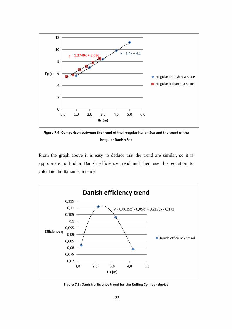
122
Figure 7.4: Comparison between the trend of the Irregular Italian Sea and the trend of the
Irregular Danish Sea
From the graph above it is easy to deduce that the trend are similar, so it is
appropriate to find a Danish efficiency trend and then use this equation to
calculate the Italian efficiency.
Figure 7.5: Danish efficiency trend for the Rolling Cylinder device
y = 1,4x + 4,2 y = 1,2749x + 5,016
0
2
4
6
8
10
12
0,0 1,0 2,0 3,0 4,0 5,0 6,0
Tp (s)
Hs (m)
Irregular Danish sea state
Irregular Italian sea state
y = 0,0035x3 - 0,05x2 + 0,2125x - 0,171
0,07
0,075
0,08
0,085
0,09
0,095
0,1
0,105
0,11
0,115
1,8 2,8 3,8 4,8 5,8
Efficiency
Hs (m)
Danish efficiency trend
Danish efficiency trend

123
With the equation representing the Danish trend it is possible to calculate the
efficiency in the Italian sea.
y = Efficiency x = Hs (from wave state in Mazara del Vallo)
-0,120945313 0,25
-0,038273438 0,75
0,023335938 1,25
0,066507813 1,75
0,093867188 2,25
0,108039063 2,75 Table 7.4: Efficiency for the Italian Sea
For the first and the second wave state the efficiency is negative. It means that for
these wave states the device does not produce and its power production is zero.
Figure 7.6: Danish efficiency trend and Italian efficiency trend
Note the efficiency all the data are available to calculate the yearly energy wave
power, the yearly energy power production and the overall efficiency as we did in
the previous chapter.
-0,15
-0,1
-0,05
0
0,05
0,1
0,15
0 1 2 3 4 5 6
Effi
cie
ncy
Hs (m)
Danish efficiency trend
Italian efficiency trend

124
WS H [m]
Tp [s] P wave [KW/m]
Prob. Prob.*Pwave [KW/m]
Eff. Pgen [kW/m] Pgen.*Prob. [KW/m]
1 0,25 5,48 0,13 0,268 0,03 0 0,00 0,00
2 0,75 5,78 1,23 0,3339 0,41 0 0,00 0,00
3 1,25 6,63 3,91 0,1928 0,75 0,023 0,09 0,02
4 1,75 7,24 8,37 0,1074 0,90 0,067 0,56 0,06
5 2,25 7,88 15,05 0,0492 0,74 0,094 1,41 0,07
6 2,75 8,56 24,41 0,0244 0,60 0,108 2,64 0,06
Table 7.5: Summarize of the performance of the Rolling Cylinder in irregular waves, in full scale
and in an Italian installation
From the values in the table above, the parameters were calculated in order to
have an idea of the performance of the device:
- Yearly average wave power =
5
1
)*(PrWs
Pwaveob = (7.2.1)
= 0,03+0,41+0,75+0,90+0,74+0,60 = 3,43 kW/m
-Yearly average power production =
5
1
)*(PrWs
Pgenob = (7.2.2)
= 0,02+0,06+0,07+0,06 = 0,21 kW/m
-Overall efficiency = power waveaverageYearly
productionpower averageYearly = (7.2.3)
=
= 0,06
-Yearly energy power production = Yearly average power production* 365*24
(7.2.4)
= 0,21*365*24 = 1,84 MWh/y/m

125
Yearly average wave power [kW/m] 3,43
Yearly average power production [kW/m] 0,21
Overall efficiency 0,06
Yearly energy power production [MWh/y/m] 1,84
Table 7.6: Summary of the performance of the Rolling Cylinder wave energy converter in
irregular waves, in full scale and in an Italian installation
7.3 Comparison between a hypothetical farm of Rolling Cylinder and
Wave Piston devices
The aim of this part is to drawn a comparison between the yearly energy power
production of a Rolling Cylinder device’s farm and the yearly energy power
production of a Wave Piston device’s farm.
The Wave Piston is a device similar to the Rolling Cylinder.
The Wave Piston is a new WEC belonging to the OWC category, invented by a
Danish group including Martin Von Bülow and Kristian Glejbøl, from
Copenhagen. This near-shore floating device is composed of large and thin plates
(i.e. energy collectors) placed perpendicularly to the sea bottom.
These plates can slide back and forth along a static structure, constituted by a
pipe, and are kept in place by a spring. The pipe transports the pressurized sea-
water to the turbine station.
Experiments to investigate the power production were carried out in February
2010, in the deep water wave basin of the Department of Civil Engineering, Water
and Soil, at Aalborg University (DK) [30].
The full-scale Wave Piston is intended to have a floating structure with a flexible
mooring whereas the down-scaled device has a fixed structure (2.40 m long)
composed by a support structure with iron “legs” and attached 4 collectors. These
collectors (each 0.5m wide and 0.1m high) in the model rotate instead of translate.
In order to reduce the effect of an arm rotating around a fixed pivot, the legs are
sufficiently lengthy.

126
Figure 7.7: Wave Piston prototype in scale 1:30 in the laboratory of Aalborg University
Figure 7.8: Simulation of the device in the real sea Figure 7.9: A plate of the Wave Piston

127
The tables below show the output energy of the Wave Piston wave energy
converter for an hypothetical installation in Mazara del Vallo. The yearly
available average wave power is 3,43 kW/m and the yearly power generated is
about 0,30 kW/m compared to 0,21 kW/m of the Rolling Cylinder, corresponding
to a yearly energy production per meter of 2,63 MWh/y/m compared to the
Rolling Cylinder of 1,84 MWh/y/m [31].
WS Hs [m]
Tp [s] P wave (KW/m)
Prob. Prob.*Pwave Eff. Pgen [kW/m]
Pgen.*Prob.
1 0,25 5,48 1,94 0,268 0,52 0,22 0,4268 0,114
2 0,75 5,78 18,4 0,3339 6,14 0,160 2,9440 0,983
3 1,25 6,63 58,58 0,1928 11,29 0,110 6,4438 1,242
4 1,75 7,24 125,49 0,1074 13,48 0,080 10,0392 1,078
5 2,25 7,88 225,68 0,0492 11,10 0,060 13,5408 0,666
6 2,75 8,56 366,09 0,0244 8,93 0,040 14,6436 0,357
Table 7.7: Summary of the performance of the Wave Piston wave energy converter in an Italian
installation. The value of the power that can be converted from the waves into useful
mechanical power by the Wave Piston model is referred to one plate of 15m of width . The
device is subjected to irregular wave [31]
Yearly average wave power [kW/m] 3,43
Yearly average power production [kW/m] 0,30
Overall efficiency 0,09
Yearly energy power production [MWh/y/m] 2,63
Table 7.8: Summary of the performance of the Wave Piston wave energy converter in irregular
waves, in full scale and in an Italian installation [31]
The goal of this part is to realize a wave energy converter farm whose dimensions
are about 2 km longshore and 500 meters crosshore. To calculate the yearly
energy power production of this farm we need to calculate the yearly energy
power production of one Rolling Cylinder’s device and the yearly energy power
production of one Wave Piston’s device and then compare the two results.

128
ROLLING CYLINDER
Yearly energy power production 1,84 MWh/y/m
Width of the device 11 m
Yearly energy power production for each device 20,24 MWh/y
WAVE PISTON
Yearly energy power production 2,63 MWh/y/m
Width of the device 15 m
Collectors for each device 4
Yearly energy power production for each device 157,8 MWh/y Table 7.9: Comparison between the performance of the Rolling Cylinder device and the Wave
Piston device
For the Wave Piston, 4 collectors are considered because measurements for each
plate were done and the energy power production was almost the same for each
collector.
To calculate the yearly energy production of that farm, it is necessary to know the
real dimensions in full scale of each device in order to calculate how many device
it is possible to place in a farm of that dimensions (2 km length and 500 m width).
Note the number of the devices and the yearly energy power production of each
device it is easy to calculate the yearly energy power production for the whole
farm.
ROLLING CYLINDER
Length of the device (1:25) 4,44 m
Length of the device (1:1) 111 m
Width of the device (1:25) 0,44 m
Width of the device (1:1) 11 m
WAVE PISTON
Length of the device (1:30) 2,40 m
Length of the device (1:1) 72 m
Width of the device (1:30) 0,5 m
Width of the device (1:1) 15 m Table 7.10: Dimension in full scale of the Rolling Cylinder device and Wave Piston device
For planning an hypothetical farm of Rolling Cylinder devices, it is supposed to
realize a farm whose dimensions are 1943 m longshore and 555 m crosshore. In
this way it is possible to place 3 rows of device crosshore and 70 devices for each

129
row, for a total amount of 210 devices. If each device produce 20,24 MWh/y and
each family average need 8kWh/d, this farm can supplied about 1456 families.
The distance between two devices is 17 m and the distance between two rows is
111 m.
Figure 7.10: An hypothetical farm of Rolling Cylinder devices in the Mediterranean Sea, Mazara
del Vallo
Figure 7.11: 3D-Rendering of the Rolling Cylinder device in the real sea

130
ROLLING CYLINDER
Dimensions of the farm 1943*555 m2
Number of devices in the farm 210
Yearly energy production of each device 20,24 MWh/y
Yearly energy production of the whole farm 4250,4 MWh/y
Daily energy demand for a family 8 kWh/d
Number of families supplied 1456 Table 7.11: Summary of the performance of an hypothetical farm of Rolling Cylinder devices
Regarding an hypothetical farm of Wave Piston devices, it is supposed to realize
a farm whose dimensions are 1953 m longshore and 504 m crosshore. In this way
it is possible to place 4 rows of device crosshore and 52 devices for each row, for
a total amount of 208 devices. If each device produce 157,8 MWh/y and each
family average need 8kWh/d, this farm can satisfy about 11240 families.
The distance between two devices is 23 m and the distance between two rows is
72 m.
Figure 7.12: An hypothetical farm of Wave Piston devices in the Mediterranean Sea, Mazara del
Vallo

131
Figure 7.13: 3D-Rendering of the Rolling Cylinder device in the real sea
WAVE PISTON
Dimensions of the farm 1953*504 m2
Number of devices in the farm 208
Yearly energy production of each device 157,8 MWh/y
Yearly energy production of the whole farm 32822,4 MWh/y
Daily energy demand for a family 8 kWh/y
Number of families supplied 11241 Table 7.12: Summary of the performance of an hypothetical farm of Wave Piston devices

132

133
8. Conclusion
The goal of this thesis was to optimize the design of the new wave energy
converter: Rolling Cylinder and then analyze the performance and the power
production of that device.
The best overall configuration of the device was achieved running all the tests
under regular waves, using the “short model” device in scale 1:25 (1,4 m in length
and 0,44 m wide). The results are shown below:
Best fin thickness; 0,75 mm
Best number of fin sets mounted on the model: 7 sets.
The difference, in term of efficiency, between 7 sets and 4 sets is almost
negligible. It is possible to delve into this aspect and maybe from the
economic point of view is better to put 4 sets. In this way the power
production is less but it is possible to save money.
Best number of fins par set: 6 fins par set
Best buoyancy level: 14 cm.
This means that half of the fin is submerged. It is also possible to elaborate
this aspect because if the power loss between 14 cm and 22 cm is low is
better to use the buoyancy level 22. In this case the fins are totally
submerged and they are safer during a storm.
Fin thickness Fin sets mounted
on the model
Fins par set Buoyancy level
0,75 mm 7 sets 6 fins 14 cm (half of the
fin submerged)
Table 8.1 : Design optimization under regular waves

134
After the design optimization of the short model, a full length model of the
Rolling Cylinder device in scale 1:25 was constructed, to achieve the second
objective of this project, hence evaluate the potential power production.
The total length of the “full length model” is 4,44 m with 11 set of fins of 0.75
mm thickness, 6 fins par set and distance between one set and the other of 40 cm.
The device was placed in the middle of the deep wave basin at AAU laboratory
with d=0.65 m water depth and all the tests were run under irregular waves. The
results are shown in the table below.
Wave State Efficiency
1 0,0317
2 0,082
3 0,111
4 0,103
5 0,079
Table 8.2: Efficiency of the device under irregular waves
The yearly energy power production obtained under irregular waves was 10
MWh/y/m with an efficiency of 0,09. This result is lower in comparison with the
yearly energy production obtained in regular waves that was 21,9 MWh/y/m. The
difference can be explained by the fact that the optimized “short” model had 7 set
of fins and the “full length model” (3 times longer than the short model) had 11
set of fins instead of 21. So the yearly energy production should be the double, 20
MWh/y/m. Since the tests with 21 set of fins were not run, it would be better
advised to use a factor of safety equal to 2/3 and write that the yearly energy
power production under irregular is 15MWh/y/m with a factor of safety equal to
2/3.

135
Moreover, to be borne out of the facts and to understand better the performance of
the Rolling Cylinder, an hypothetical application of this device in the
Mediterranean Sea was done.
The result are shown in the table below.
Yearly average wave power [kW/m] 3,43
Yearly average power production [kW/m] 0,21
Overall efficiency 0,06
Yearly energy power production [MWh/y/m] 1,84
Table 8.3: Summary of the performance of the Rolling Cylinder wave energy converter under
irregular waves, in full scale and in an Italian installation, Mazara del Vallo
The yearly energy power production of 1,84 MWh/y/m was obtained doing the
calculation with the yearly energy production in the Danish sea equal to
10MWh/y/m. If this value is higher also the energy in the Italian sea increase and
it is equal to 2,76 MWh/y/m.
To match expectations, the performance of the device and the power production in
the Mediterranean Sea are lower than in the Danish Sea, but it is interesting to
notice that Rolling Cylinder is comparable with Wave Piston device that has a
similar performance and a similar geometrical configuration of the Rolling
Cylinder.
Yearly average wave power [kW/m] 3,43
Yearly average power production [kW/m] 0,30
Overall efficiency 0,09
Yearly energy power production [MWh/y/m] 2,63
Table 8.4: Summary of the performance of the Wave Piston wave energy converter under
irregular waves, in full scale and in an Italian installation, Mazara del Vallo
Hence, the last step is to draw a comparison between a hypothetical farm of
Rolling Cylinder and Wave Piston devices.

136
Setting the dimensions of the farm, note the dimensions of the device in full scale
and the yearly energy production of each device, it is easy to calculate how many
families can be supplied from these two farms.
ROLLING CYLINDER
Dimensions of the farm 1943*555 m2
Number of devices in the farm 210
Yearly energy production of each device 28,5 MWh/y
Yearly energy production of the whole farm 6006 MWh/y
Daily energy demand for a family 8 kWh/d
Number of families supplied 2057 Table 8.5: Summary of the performance of an hypothetical farm of Rolling Cylinder devices
WAVE PISTON
Dimension of the farm 1953*504 m2
Number of devices in the farm 208
Yearly energy production of each device 157,8 MWh/y
Yearly energy production of the whole farm 32822,4 MWh/y
Daily energy demand for a family 8 kWh/d
Number of families supplied 11241 Table 8.6: Summary of the performance of an hypothetical farm of Wave Piston devices
Of course this is only the first phase of the whole assessment of the device.
In the proof of concept a lot of aspects are not take into consideration, like the
mooring of the device, the material of the device in full-scale, the accumulation of
marine organism on the device and the PTO system. This does not mean that they
are not important but if they are negligible in the first phase they are necessary
since the second phase of the assessment of the device.

137
Appendix A: Data Processing
Thickness= 0,4 mm (4 set, 6 fins)
RW 4 (H=0,113 m T=1,960 s)
Load (N) Efficiency
1 0,093
1,7 0,06522
7 0,03987
0
0,05
0,1
0,15
0 2 4 6 8
Efficiency
Load [N]
Thickness= 0,4 mm (4 set, 6 fins)
RW 4
RW 5
RW 6
RW 5 (H= 0,141 m T= 2,240 s)
Load (N) Efficiency
1 0,087
1,7 0,06
7 0,057
RW 6 (H= 0,16 m T= 1,40 s)
Load (N) Efficiency
1 0,123
1,7 0,12
7 0,114

138
Thickness= 0,75 mm (4 set, 6 fins)
RW 3 (H=0,085 m T= 1,680 s)
Mass (kg) Load (N) Time (s)
Mean Time (s) Power (W) Efficiency
Friction Weight Tot.
Mass T1 T2 T3
0,16 0,19 0,35 3,437 37,00 36,07 35,70 36,26 0,293868714 0,211861
0,16 0,24 0,4 3,928 40,68 41,45 40,63 40,92 0,297575758 0,214533
0,16 0,34 0,5 4,91 51,14 50,31 50,92 50,79 0,299684977 0,216054
0,16 0,44 0,6 5,892 73,57 70,15 69,57 71,10 0,256906559 0,185213
0,16 0,54 0,7 6,874 133,07 142,81 136,03 137,30 0,155199437 0,111889
h = 3,1 m lenght of the string g = 9,82 m/s2
d = 0,44 m fin's diameter+ cylinder's diameter
Ro = 1000 kg/m3 density of the water Tm = 1,679 s from wavelab
Hm = 0,07663 m from wavelab β = 32 for regular wave 32 P = 4,161253 W
RW 4 (H=0,113 m T=1,960 s)
Mass (kg) Load (N) Time (s)
Mean Time (s) Power (W) Efficiency
Friction Weight Tot.
Mass T1 T2 T3
0,16 0,19 0,35 3,437 20,33 20,45 20,70 20,49 0,51991054 0,15035
0,16 0,24 0,4 3,928 21,37 21,93 21,60 21,63 0,562872111 0,162774
0,16 0,34 0,5 4,91 23,95 23,16 23,04 23,38 0,650933713 0,18824
0,16 0,44 0,6 5,892 26,06 25,56 25,86 25,83 0,707222509 0,204517
0,16 0,54 0,7 6,874 31,00 29,94 32,00 30,98 0,68784377 0,198913
0,16 0,64 0,8 7,856 34,65 33,33 34 33,99 0,716422828 0,207178
0,16 0,74 0,9 8,838 42,64 41,4 42,15 42,06 0,651346382 0,188359
0,16 0,84 1 9,82 51,46 51,01 52,52 51,66 0,589238015 0,170398
0,16 0,94 1,1 10,802 66,74 70,55 63,44 66,91 0,500466298 0,144727

139
h = 3,1 m lenght of the string g = 9,82 m/s2
d = 0,44 m fin's diameter+ cylinder's diameter
Ro = 1000 kg/m3 density of the water Tm = 1,949 s from wavelab
Hm = 0,1123 m from wavelab β = 32 for regular wave 32 P = 10,37402 W
Time (s) Lenght (m) Velocity (m/s) Radius (m) W (rad/s)
20,49333 3,1 0,151268705 0,06 2,521145
21,63333 0,143297381 2,38829
23,38333 0,132573058 2,209551
25,82667 0,120030976 2,000516
30,98 0,100064558 1,667743
33,99333 0,091194352 1,519906
42,06333 0,073698391 1,228307
51,66333 0,060003871 1,000065
66,91 0,046330892 0,772182
RW 5 (H= 0,141 m T= 2,240 s)
Mass (kg) Load (N) Time (s)
Mean Time (s) Power (W) Efficiency
Friction Weight Tot.
Mass T1 T2 T3
0,16 0,19 0,35 3,437 17,11 0,622717709 0,112347
0,16 0,24 0,4 3,928 17,90 0,680268156 0,12273
0,16 0,34 0,5 4,91 19,03 0,799842354 0,144303
0,16 0,44 0,6 5,892 20,31 0,899320532 0,16225
0,16 0,54 0,7 6,874 22,53 22,84 22,78 22,72 0,938051357 0,169238
0,16 0,64 0,8 7,856 25,05 25,08 24,38 24,84 0,980550262 0,176905
0,16 0,74 0,9 8,838 26,98 26,09 26,5 26,52 1,032969712 0,186363
0,16 0,84 1 9,82 29,83 29,87 29,49 29,73 1,023948873 0,184735
0,16 0,94 1,1 10,802 33,05 32,77 32,22 32,68 1,024669523 0,184865
0,16 1,04 1,2 11,784 38,62 38,25 35,99 37,62 0,971036683 0,175189

140
h = 3,1 m lenght of the string g = 9,82 m/s2
d = 0,44 m fin's diameter+ cylinder's diameter
Ro = 1000 kg/m3 density of the water Tm = 2,204 s from wavelab
Hm = 0,1337 m from wavelab β = 32 for regular wave 32 P = 16,62839 W
Time (s) Lenght (m) Velocity (m/s) Radius (m) W (rad/s)
17,11 3,1 0,181180596 0,06 3,019677
17,9 0,173184358 2,886406
19,03 0,162900683 2,715011
20,31 0,15263417 2,543903
22,71667 0,136463683 2,274395
24,83667 0,124815461 2,080258
26,52333 0,11687822 1,94797
29,73 0,104271779 1,737863
32,68 0,094859241 1,580987
37,62 0,082402977 1,373383
RW 6 (H= 0,16 m T= 1,40 s)
Mass (kg) Load (N) Time (s)
Mean Time (s) Power (W) Efficiency
Friction Weight Tot.
Mass T1 T2 T3
0,16 0,19 0,35 3,437 13,08 0,814579511 0,166509
0,16 0,54 0,7 6,874 19,42 18,93 18,79 19,05 1,11879944 0,228695
0,16 0,74 0,9 8,838 21,49 21,06 20,85 21,13 1,296425868 0,265004
0,16 0,94 1,1 10,802 25,72 25,33 25,04 25,36 1,320260218 0,269876
0,16 1,04 1,2 11,784 26,25 26,18 25,83 26,09 1,400347559 0,286247

141
h = 3,1 m lenght of the string g = 9,82 m/s2
d = 0,44 m fin's diameter+ cylinder's diameter
Ro = 1000 kg/m3 density of the water Tm = 1,4 s from wavelab
Hm = 0,1576 m from wavelab β = 32 for regular wave 32 P = 14,67629 W
Time (s) Lenght (m) Velocity (m/s) Radius (m) W (rad/s)
13,08 3,1 0,237003058 0,06 3,950051
19,04667 0,162758138 2,712636
21,13333 0,146687697 2,444795
25,36333 0,122223682 2,037061
26,08667 0,118834654 1,980578
0
0,05
0,1
0,15
0,2
0,25
0,3
0,35
0 5 10 15
Efficiency
Load [N]
Thickness= 0,75 mm (4 set, 6 fins)
RW 3
RW 4
RW 5
RW 6

142
Thickness= 1 mm (4 set, 6 fins)
RW 3 (H=0,085 m T= 1,680 s) the device does not turn
RW 4 (H=0,113 m T=1,960 s)
Mass (kg) Load (N) Time (s)
Mean Time (s)
Power (W) Efficiency
Friction Weight Tot.
Mass T1 T2 T3
0,16 0,19 0,35 3,437 32,70 33,50 33,20 33,13 0,3215704 0,095557
0,16 0,24 0,4 3,928 35,30 35,00 35,10 35,13 0,3465882 0,102991
0,16 0,34 0,5 4,91 47,10 47,10 46,60 46,93 0,3243111 0,096371
0,16 0,44 0,6 5,892 69,80 67,20 66,70 67,90 0,2690015 0,079936
0,16 0,54 0,7 6,874 109,80 107,90 99,00 105,57 0,2018573 0,059983
h = 3,1 m
g = 9,82 s
d = 0,44 m
Ro = 1000 kg/m3
Tm = 1,959 s
Hm = 0,1105 m
β = 32
P = 10,09566 W

143
RW 5 (H= 0,141 m T= 2,240 s)
Mass (kg) Load (N) Time (s)
Mean Time (s)
Power (W) Efficiency
Friction Weight Tot.
Mass T1 T2 T3
0,16 0,19 0,35 3,437 23,44 23,00 24,03 23,49 0,4535845 0,082605
0,16 0,24 0,4 3,928 25,02 25,51 24,70 25,08 0,4855829 0,088433
0,16 0,34 0,5 4,91 29,43 29,61 29,79 29,61 0,5140493 0,093617
0,16 0,44 0,6 5,892 34,42 35,68 35,14 35,08 0,5206727 0,094823
0,16 0,54 0,7 6,874 41,35 41,29 42,59 41,74 0,5104863 0,092968
0,16 0,64 0,8 7,856 55,66 54,9 56,56 55,71 0,4371757 0,079617
0,16 0,74 0,9 8,838 76 76 76,00 0,3604974 0,065653
h = 3,1 m
g = 9,82 s
d = 0,44 m
Ro = 1000 kg/m3
Tm = 2,24 s
Hm = 0,132 m
β = 32
P = 16,47296 W
RW 6 (H= 0,16 m T= 1,40 s)
Mass (kg) Load (N) Time (s)
Mean Time (s)
Power (W) Efficiency
Friction Weight Tot.
Mass T1 T2 T3
0,16 0,19 0,35 3,437 17,50 16,78 16,83 17,04 0,6253982 0,144673
0,16 0,24 0,4 3,928 17,64 17,73 17,46 17,61 0,6914708 0,159958
0,16 0,34 0,5 4,91 19,08 19,21 19,12 19,14 0,7953841 0,183996
0,16 0,44 0,6 5,892 21,16 21,28 21,46 21,30 0,8575211 0,19837
0,16 0,54 0,7 6,874 23,44 23,49 23,26 23,40 0,9107879 0,210692
0,16 0,64 0,8 7,856 25,56 25,87 25,74 25,72 0,9467513 0,219012
0,16 0,74 0,9 8,838 29,79 29,16 29,2 29,38 0,9324265 0,215698
0,16 0,94 1,1 10,802 42,88 43,42 41,53 42,61 0,7858766 0,181797
0,16 1,04 1,2 11,784 56,02 54,04 52,65 54,24 0,673537 0,155809
0,16 1,24 1,4 13,748 106,1 99,4 102,75 0,4147815 0,095951

144
h = 3,1 m
g = 9,82 s
d = 0,44 m
Ro = 1000 kg/m3
Tm= 1,399 s
Hm = 0,1482 m
β = 32
P = 12,96851 W
Set of fins = 4 (0,75 mm, 6 fins)
RW 3 (H=0,085 m T= 1,680 s)
Mass (kg) Load (N) Time (s)
Mean Time (s) Power (W) Efficiency
Friction Weight Tot.
Mass T1 T2 T3
0,16 0,19 0,35 3,437 37,00 36,07 35,70 36,26 0,293868714 0,211861
0,16 0,24 0,4 3,928 40,68 41,45 40,63 40,92 0,297575758 0,214533
0,16 0,34 0,5 4,91 51,14 50,31 50,92 50,79 0,299684977 0,216054
0,16 0,44 0,6 5,892 73,57 70,15 69,57 71,10 0,256906559 0,185213
0,16 0,54 0,7 6,874 133,07 142,81 136,03 137,30 0,155199437 0,111889
0
0,05
0,1
0,15
0,2
0,25
0 5 10 15
Efficiency
Load [N]
Thickness = 1 mm (4 set, 6 fins)
RW 4
RW 5
RW 6

145
h = 3,1 m
g = 9,82 s
d = 0,44 m
Ro = 1000 kg/m3
Tm = 1,679 s
Hm = 0,07663 m
β = 32
P = 4,161253 W
RW 4 (H=0,113 m T=1,960 s)
Mass (kg) Load (N) Time (s)
Mean Time (s) Power (W) Efficiency
Friction Weight Tot.
Mass T1 T2 T3
0,16 0,19 0,35 3,437 20,33 20,45 20,70 20,49 0,51991054 0,15035
0,16 0,24 0,4 3,928 21,37 21,93 21,60 21,63 0,562872111 0,162774
0,16 0,34 0,5 4,91 23,95 23,16 23,04 23,38 0,650933713 0,18824
0,16 0,44 0,6 5,892 26,06 25,56 25,86 25,83 0,707222509 0,204517
0,16 0,54 0,7 6,874 31,00 29,94 32,00 30,98 0,68784377 0,198913
0,16 0,64 0,8 7,856 34,65 33,33 34 33,99 0,716422828 0,207178
0,16 0,74 0,9 8,838 42,64 41,4 42,15 42,06 0,651346382 0,188359
0,16 0,84 1 9,82 51,46 51,01 52,52 51,66 0,589238015 0,170398
0,16 0,94 1,1 10,802 66,74 70,55 63,44 66,91 0,500466298 0,144727
h = 3,1 m
g = 9,82 s
d = 0,44 m
Ro = 1000 kg/m3
Tm = 1,949 s
Hm = 0,1123 m
β = 32
P = 10,37402 W

146
RW 5 (H= 0,141 m T= 2,240 s)
Mass (kg) Load (N) Time (s)
Mean Time (s) Power (W) Efficiency
Friction Weight Tot.
Mass T1 T2 T3
0,16 0,19 0,35 3,437 17,11 0,622717709 0,112347
0,16 0,24 0,4 3,928 17,90 0,680268156 0,12273
0,16 0,34 0,5 4,91 19,03 0,799842354 0,144303
0,16 0,44 0,6 5,892 20,31 0,899320532 0,16225
0,16 0,54 0,7 6,874 22,53 22,84 22,78 22,72 0,938051357 0,169238
0,16 0,64 0,8 7,856 25,05 25,08 24,38 24,84 0,980550262 0,176905
0,16 0,74 0,9 8,838 26,98 26,09 26,5 26,52 1,032969712 0,186363
0,16 0,84 1 9,82 29,83 29,87 29,49 29,73 1,023948873 0,184735
0,16 0,94 1,1 10,802 33,05 32,77 32,22 32,68 1,024669523 0,184865
0,16 1,04 1,2 11,784 38,62 38,25 35,99 37,62 0,971036683 0,175189
h = 3,1 m
g = 9,82 s
d = 0,44 m
Ro = 1000 kg/m3
Tm = 2,204 s
Hm = 0,1337 m
β = 32
P = 16,62839 W
RW 6 (H= 0,16 m T= 1,40 s)
Mass (kg) Load (N) Time (s)
Mean Time (s) Power (W) Efficiency
Friction Weight Tot.
Mass T1 T2 T3
0,16 0,19 0,35 3,437 13,08 0,814579511 0,166509
0,16 0,54 0,7 6,874 19,42 18,93 18,79 19,05 1,11879944 0,228695
0,16 0,74 0,9 8,838 21,49 21,06 20,85 21,13 1,296425868 0,265004
0,16 0,94 1,1 10,802 25,72 25,33 25,04 25,36 1,320260218 0,269876
0,16 1,04 1,2 11,784 26,25 26,18 25,83 26,09 1,400347559 0,286247

147
h = 3,1 m
g = 9,82 s
d = 0,44 m
Ro = 1000 kg/m3
Tm = 1,4 s
Hm = 0,1576 m
β = 32
P = 14,67629 W
Set of fins = 7 (0,75 mm, 6 fins)
RW 3 (H=0,085 m T= 1,680 s)
Mass (kg) Load (N) Time (s)
Mean Time (s) Power (W) Efficiency
Friction Weight Tot.
Mass T1 T2 T3
0,2 0,14 0,34 3,3388 45,13 44,19 38,47 42,60 0,242983332 0,225635
0,2 0,24 0,44 4,3208 53,19 56,92 58,54 56,22 0,238265283 0,221254
0,2 0,34 0,54 5,3028 60,61 57,51 57,15 58,42 0,281371826 0,261283
0,2 0,44 0,64 6,2848 93,06 92,29 93,96 93,10 0,209260821 0,19432
0
0,05
0,1
0,15
0,2
0,25
0,3
0,35
0 5 10 15
Efficiency
Load [N]
4 set of fins (0,75 mm, 6 fins)
RW 3
RW 4
RW 5
RW 6

148
h = 3,1 m
g = 9,82 s
d = 0,44 m
Ro = 1000 kg/m3
Tm = 1,679 s
Hm = 0,06752 m
β = 32
P = 3,230661 W
Time (s) Lenght (m) Velocity (m/s) Radius (m) W (rad/s)
42,59666667 3,1 0,072775648 0,06 1,212927459
56,21666667 0,055143789 0,919063149
58,42333333 0,053060992 0,88434986
93,10333333 0,033296337 0,554938957
RW 4 (H=0,113 m T=1,960 s)
Mass (kg) Load (N) Time (s)
Mean Time (s) Power (W) Efficiency
Friction Weight Tot.
Mass T1 T2 T3
0,2 0,24 0,44 4,3208 25,20 25,87 25,38 25,48 0,525617266 0,171672
0,2 0,34 0,54 5,3028 27,54 27,94 28,62 28,03 0,586397622 0,191523
0,2 0,44 0,64 6,2848 32,08 32,99 31,32 32,13 0,606376595 0,198049
0,2 0,54 0,74 7,2668 35,46 36,99 35,28 35,91 0,627320524 0,204889
0,2 0,64 0,84 8,2488 38,08 38,52 37,62 38,07 0,671632289 0,219362
0,2 0,74 0,94 9,2308 47,98 46,94 46,44 47,12 0,607289474 0,198347
0,2 0,84 1,04 10,2128 54,18 50,04 52,83 52,35 0,604769436 0,197524
h = 3,1 m
g = 9,82 s
d = 0,44 m
Ro = 1000 kg/m3
Tm = 1,959 s
Hm = 0,1054 m
β = 32
P = 9,18526 W

149
Time (s) Lenght (m) Velocity (m/s) Radius (m) W (rad/s)
25,48333333 3,1 0,121648136 0,06 2,027468934
28,03333333 0,11058264 1,843043995
32,13 0,096483038 1,608050628
35,91 0,086326928 1,438782141
38,07333333 0,081421818 1,357030292
47,12 0,065789474 1,096491228
52,35 0,05921681 0,986946832
RW 5 (H= 0,141 m T= 2,240 s)
Mass (kg) Load (N) Time (s)
Mean Time (s) Power (W) Efficiency
Friction Weight Tot.
Mass T1 T2 T3
0,2 0,24 0,44 4,3208 23,17 22,95 23,44 23,19 0,577680276 0,13466
0,2 0,34 0,54 5,3028 24,61 24,70 24,75 24,69 0,66589306 0,155222
0,2 0,44 0,64 6,2848 26,82 27,28 27,58 27,23 0,715580803 0,166805
0,2 0,54 0,74 7,2668 29,92 29,66 29,29 29,62 0,760450546 0,177264
0,2 0,64 0,84 8,2488 32,22 32,08 32,07 32,12 0,796034451 0,185559
0,2 0,74 0,94 9,2308 36,27 35,73 35,77 35,92 0,796570845 0,185684
0,2 0,84 1,04 10,2128 40,18 38,92 38,78 39,29 0,805726502 0,187818
0,2 0,94 1,14 11,1948 44,77 42,16 45,52 44,15 0,786044847 0,18323
h = 3,1 m
g = 9,82 s
d = 0,44 m
Ro = 1000 kg/m3
Tm = 2,239 s
Hm = 0,1167 m
β = 32
P = 12,86979 W

150
Time (s) Lenght (m) Velocity (m/s) Radius (m) W (rad/s)
23,18666667 3,1 0,133697527 0,06 2,228292122
24,68666667 0,125573859 2,092897651
27,22666667 0,113858962 1,897649363
29,62333333 0,104647238 1,744120626
32,12333333 0,096503061 1,608384352
35,92333333 0,086294887 1,438248121
39,29333333 0,07889379 1,314896505
44,15 0,070215176 1,170252926
RW 6 (H= 0,16 m T= 1,40 s)
Mass (kg) Load (N) Time (s)
Mean Time (s) Power (W) Efficiency
Friction Weight Tot.
Mass T1 T2 T3
0,2 0,34 0,54 5,3028 17,32 16,60 17,14 17,02 0,965844888 0,272689
0,2 0,44 0,64 6,2848 17,91 17,95 18,00 17,95 1,085195693 0,306385
0,2 0,54 0,74 7,2668 18,58 18,99 19,30 18,96 1,188346052 0,335508
0,2 0,64 0,84 8,2488 20,49 20,25 20,16 20,30 1,259668966 0,355645
0,2 0,74 0,94 9,2308 21,46 21,64 20,16 21,09 1,357041416 0,383136
0,2 0,84 1,04 10,2128 22,34 22,18 21,78 22,10 1,432564706 0,404459
0,2 0,94 1,14 11,1948 23,34 23,31 23,54 23,40 1,483283089 0,418778
0,2 1,04 1,24 12,1768 25,2 24,3 24,97 24,82 1,520669263 0,429333
0,2 1,14 1,34 13,1588 25,34 24,88 25,3 25,17 1,620456038 0,457506
0,2 1,24 1,44 14,1408 26,31 27,2 26,43 26,65 1,645101826 0,464465
0,2 1,34 1,54 15,1228 28,04 1,671921541 0,472037
0,2 1,44 1,64 16,1048 29,93 28,92 30,48 29,78 1,676644352 0,47337
0,2 1,54 1,74 17,0868 32,25 32,37 32,18 32,27 1,641603719 0,463477
h = 3,1 m
g = 9,82 s
d = 0,44 m
Ro = 1000 kg/m3
Tm = 1,4 s
Hm = 0,1341 m
β = 32
P = 10,62579 W

151
Time (s) Lenght (m) Velocity (m/s) Radius (m) W (rad/s)
17,02 3,1 0,18213866 0,06 3,03564434
17,95333333 0,172669885 2,877831415
18,95666667 0,16353086 2,725514331
20,3 0,15270936 2,545155993
21,08666667 0,14701233 2,450205501
22,1 0,140271493 2,33785822
23,39666667 0,132497507 2,208291779
24,82333333 0,124882503 2,08137505
25,17333333 0,123146186 2,052436441
26,64666667 0,116337253 1,938954216
28,04 0,110556348 1,842605801
29,77666667 0,104108362 1,735139371
32,26666667 0,09607438 1,601239669
0
0,05
0,1
0,15
0,2
0,25
0,3
0,35
0,4
0,45
0,5
0 5 10 15 20
Efficiency
Load [N]
7 set of fins (0,75 mm, 6 fins)
RW 3
RW 4
RW 5
RW 6

152
Set of fins = 3 (0,75 mm, 6 fins)
RW 3 (H=0,085 m T= 1,680 s)
Mass (kg) Load (N) Time (s)
Mean Time (s) Power (W) Efficiency
Friction Weight Tot.
Mass T1 T2 T3
0,13 0,04 0,17 1,6694 32,08 32,4 32,87 32,45 0,159480431 0,12941
0,13 0,09 0,22 2,1604 37,32 37,58 36,94 37,28 0,179646996 0,145774
0,13 0,14 0,27 2,6514 47,90 45,87 50,27 48,01 0,171188698 0,13891
0,13 0,24 0,37 3,6334 158,26 178,70 144,73 160,56 0,070150138 0,056923
h = 3,1 m
g = 9,82 s
d = 0,44 m
Ro = 1000 kg/m3
Tm = 1,679 s
Hm = 0,07223 m
β = 32
P = 3,697105 W
RW 4 (H=0,113 m T=1,960 s)
Mass (kg) Load (N) Time (s)
Mean Time (s) Power (W) Efficiency
Friction Weight Tot.
Mass T1 T2 T3
0,13 0,14 0,27 2,6514 20,83 21,25 21,65 21,24 0,386913855 0,106523
0,13 0,24 0,37 3,6334 25,01 24,98 26,04 25,34 0,444437985 0,12236
0,13 0,34 0,47 4,6154 30,10 30,40 30,68 30,39 0,470752577 0,129604
0,13 0,44 0,57 5,5974 39,08 40,72 39,25 39,68 0,437260143 0,120384
0,13 0,54 0,67 6,5794 50,55 54,81 54,16 53,17 0,38357836 0,105604
0,13 0,64 0,77 7,5614 68,53 72,74 75,72 72,33 0,324074934 0,089222

153
h = 3,1 m
g = 9,82 s
d = 0,44 m
Ro = 1000 kg/m3
Tm = 1,959 s
Hm = 0,1148 m
β = 32
P = 10,89668 W
RW 5 (H= 0,141 m T= 2,240 s)
Mass (kg) Load (N) Time (s)
Mean Time (s) Power (W) Efficiency
Friction Weight Tot.
Mass T1 T2 T3
0,13 0,14 0,27 2,6514 19,81 17,89 18,65 18,78 0,437586868 0,07351
0,13 0,24 0,37 3,6334 20,86 20,59 21,05 20,83 0,54064992 0,090823
0,13 0,34 0,47 4,6154 24,49 23,90 24,59 24,33 0,588150452 0,098803
0,13 0,44 0,57 5,5974 29,84 30,35 29,51 29,90 0,580332441 0,097489
0,13 0,54 0,67 6,5794 33,86 34,32 34,04 34,07 0,598595383 0,100557
0,13 0,64 0,77 7,5614 39,42 40,28 41,34 40,35 0,580973397 0,097597
0,13 0,74 0,87 8,5434 49,66 48,84 51,38 49,96 0,530114892 0,089053
h = 3,1 m
g = 9,82 s
d = 0,44 m
Ro = 1000 kg/m3
Tm = 2,238 s
Hm = 0,1375 m
β = 32
P = 17,85835 W

154
RW 6 (H= 0,16 m T= 1,40 s)
Mass (kg) Load (N) Time (s)
Mean Time (s) Power (W) Efficiency
Friction Weight Tot.
Mass T1 T2 T3
0,13 0,24 0,37 3,6334 17,44 17,50 17,74 17,56 0,641431663 0,128263
0,13 0,44 0,57 5,5974 20,84 21,64 19,55 20,68 0,839203934 0,16781
0,13 0,54 0,67 6,5794 20,87 21,45 22,50 21,61 0,943974391 0,188761
0,13 0,64 0,77 7,5614 25,82 22,91 23,87 24,20 0,968609091 0,193687
0,13 0,74 0,87 8,5434 26,41 29,28 26,49 27,39 0,966824288 0,19333
0,13 0,84 0,97 9,5254 30,18 28,89 30,47 29,85 0,989348001 0,197834
0,13 0,94 1,07 10,5074 36,38 36,43 38,34 37,05 0,879161673 0,1758
0,13 1,04 1,17 11,4894 40,15 40,42 41,41 40,66 0,875974914 0,175163
0,13 1,14 1,27 12,4714 45,69 45,83 45,81 45,78 0,844564334 0,168882
h = 3,1 m
g = 9,82 s
d = 0,44 m
Ro = 1000 kg/m3
Tm = 1,399 s
Hm = 0,1594 m
β = 32
P = 15,00273 W

155
Fins per set = 6 ( 0,75 mm, 7 set)
RW 3 (H=0,085 m T= 1,680 s)
Mass (kg) Load (N) Time (s)
Mean Time (s) Power (W) Efficiency
Friction Weight Tot.
Mass T1 T2 T3
0,2 0,14 0,34 3,3388 45,13 44,19 38,47 42,60 0,242983332 0,225635
0,2 0,24 0,44 4,3208 53,19 56,92 58,54 56,22 0,238265283 0,221254
0,2 0,34 0,54 5,3028 60,61 57,51 57,15 58,42 0,281371826 0,261283
0,2 0,44 0,64 6,2848 93,06 92,29 93,96 93,10 0,209260821 0,19432
0
0,05
0,1
0,15
0,2
0,25
0 0,5 1 1,5 2 2,5 3 3,5 4 4,5 5 5,5 6 6,5 7 7,5 8 8,5 9 9,5 10 10,5 11 11,5 12 12,5 13 13,5
Efficiency
Load [N]
3 set of fins (0,75 mm, 6 fins)
RW 3
RW 4
RW 5
RW 6

156
h = 3,1 m
g = 9,82 s
d = 0,44 m
Ro = 1000 kg/m3
Tm = 1,679 s
Hm = 0,06752 m
β = 32
P = 3,230661 W
RW 4 (H=0,113 m T=1,960 s)
\
Mass (kg) Load (N) Time (s)
Mean Time (s) Power (W) Efficiency
Friction Weight Tot.
Mass T1 T2 T3
0,2 0,24 0,44 4,3208 25,20 25,87 25,38 25,48 0,525617266 0,171672
0,2 0,34 0,54 5,3028 27,54 27,94 28,62 28,03 0,586397622 0,191523
0,2 0,44 0,64 6,2848 32,08 32,99 31,32 32,13 0,606376595 0,198049
0,2 0,54 0,74 7,2668 35,46 36,99 35,28 35,91 0,627320524 0,204889
0,2 0,64 0,84 8,2488 38,08 38,52 37,62 38,07 0,671632289 0,219362
0,2 0,74 0,94 9,2308 47,98 46,94 46,44 47,12 0,607289474 0,198347
0,2 0,84 1,04 10,2128 54,18 50,04 52,83 52,35 0,604769436 0,197524
h = 3,1 m
g = 9,82 s
d = 0,44 m
Ro = 1000 kg/m3
Tm = 1,959 s
Hm = 0,1054 m
β = 32
P = 9,18526 W

157
Time (s) Lenght (m) Velocity (m/s) Radius (m) W (rad/s)
25,4833 3,1 0,121648136 0,06 2,027469
28,0333 0,11058264 1,843044
32,13 0,096483038 1,608051
35,91 0,086326928 1,438782
38,0733 0,081421818 1,35703
47,12 0,065789474 1,096491
52,35 0,05921681 0,986947
RW 5 (H= 0,141 m T= 2,240 s)
Mass (kg) Load (N) Time (s)
Mean Time (s) Power (W) Efficiency
Friction Weight Tot.
Mass T1 T2 T3
0,2 0,24 0,44 4,3208 23,17 22,95 23,44 23,19 0,577680276 0,13466
0,2 0,34 0,54 5,3028 24,61 24,70 24,75 24,69 0,66589306 0,155222
0,2 0,44 0,64 6,2848 26,82 27,28 27,58 27,23 0,715580803 0,166805
0,2 0,54 0,74 7,2668 29,92 29,66 29,29 29,62 0,760450546 0,177264
0,2 0,64 0,84 8,2488 32,22 32,08 32,07 32,12 0,796034451 0,185559
0,2 0,74 0,94 9,2308 36,27 35,73 35,77 35,92 0,796570845 0,185684
0,2 0,84 1,04 10,2128 40,18 38,92 38,78 39,29 0,805726502 0,187818
0,2 0,94 1,14 11,1948 44,77 42,16 45,52 44,15 0,786044847 0,18323
h = 3,1 m
g = 9,82 s
d = 0,44 m
Ro = 1000 kg/m3
Tm = 2,239 s
Hm = 0,1167 m
β = 32
P = 12,86979 W

158
Time (s) Lenght (m) Velocity (m/s) Radius (m) W (rad/s)
23,1867 3,1 0,133697527 0,06 2,228292
24,6867 0,125573859 2,092898
27,2267 0,113858962 1,897649
29,6233 0,104647238 1,744121
32,1233 0,096503061 1,608384
35,9233 0,086294887 1,438248
39,2933 0,07889379 1,314897
44,15 0,070215176 1,170253
RW 6 (H= 0,16 m T= 1,40 s)
Mass (kg) Load (N) Time (s)
Mean Time (s) Power (W) Efficiency
Friction Weight Tot.
Mass T1 T2 T3
0,2 0,34 0,54 5,3028 17,32 16,60 17,14 17,02 0,965844888 0,272689
0,2 0,44 0,64 6,2848 17,91 17,95 18,00 17,95 1,085195693 0,306385
0,2 0,54 0,74 7,2668 18,58 18,99 19,30 18,96 1,188346052 0,335508
0,2 0,64 0,84 8,2488 20,49 20,25 20,16 20,30 1,259668966 0,355645
0,2 0,74 0,94 9,2308 21,46 21,64 20,16 21,09 1,357041416 0,383136
0,2 0,84 1,04 10,2128 22,34 22,18 21,78 22,10 1,432564706 0,404459
0,2 0,94 1,14 11,1948 23,34 23,31 23,54 23,40 1,483283089 0,418778
0,2 1,04 1,24 12,1768 25,2 24,3 24,97 24,82 1,520669263 0,429333
0,2 1,14 1,34 13,1588 25,34 24,88 25,3 25,17 1,620456038 0,457506
0,2 1,24 1,44 14,1408 26,31 27,2 26,43 26,65 1,645101826 0,464465
0,2 1,34 1,54 15,1228 28,04 1,671921541 0,472037
0,2 1,44 1,64 16,1048 29,93 28,92 30,48 29,78 1,676644352 0,47337
0,2 1,54 1,74 17,0868 32,25 32,37 32,18 32,27 1,641603719 0,463477
h = 3,1 m
g = 9,82 s
d = 0,44 m
Ro = 1000 kg/m3
Tm = 1,4 s
Hm = 0,1341 m
β = 32
P = 10,62579 W

159
Time (s) Lenght (m) Velocity (m/s) Radius (m) W (rad/s)
17,02 3,1 0,18213866 0,06 3,035644
17,9533 0,172669885 2,877831
18,9567 0,16353086 2,725514
20,3 0,15270936 2,545156
21,0867 0,14701233 2,450206
22,1 0,140271493 2,337858
23,3967 0,132497507 2,208292
24,8233 0,124882503 2,081375
25,1733 0,123146186 2,052436
26,6467 0,116337253 1,938954
28,04 0,110556348 1,842606
29,7767 0,104108362 1,735139
32,2667 0,09607438 1,60124
0
0,05
0,1
0,15
0,2
0,25
0,3
0,35
0,4
0,45
0,5
0 5 10 15 20
Efficiency
Load [N]
7 fins per set ( 0,75 mm, 7 set)
RW 3
RW 4
RW 5
RW 6

160
Fins per set = 3 ( 0,75 mm, 7 set)
RW 3 (H=0,085 m T= 1,680 s) does not turn RW 4 (H=0,113 m T=1,960 s)
Mass (kg) Load (N) Time (s)
Mean Time (s) Power (W) Efficiency
Friction Weight Tot.
Mass T1 T2 T3
0,22 0,14 0,36 3,5352 50,57 49,94 49,89 50,13333333 0,218599468 0,060079
0,22 0,19 0,41 4,0262 54,48 51,43 49,72 51,87666667 0,240594101 0,066124
0,22 0,24 0,46 4,5172 69,50 80,42 71,33 73,75 0,189875525 0,052184
0,22 0,29 0,51 5,0082 102,59 108,13 81,26 97,33 0,159518666 0,043841
h = 3,1 m
g = 9,82 s
d = 0,44 m
Ro = 1000 kg/m3
Tm = 1,959 s
Hm = 0,1149 m
β = 32
P = 10,91567 W
RW 5 (H= 0,141 m T= 2,240 s)
Mass (kg) Load (N) Time (s)
Mean Time (s) Power (W) Efficiency
Friction Weight Tot.
Mass T1 T2 T3
0,22 0,14 0,36 3,5352 24,92 25,17 28,57 26,22 0,417967963 0,071079
0,22 0,19 0,41 4,0262 27,46 28,65 28,13 28,08 0,444487892 0,075589
0,22 0,24 0,46 4,5172 32,76 37,00 36,70 35,49 0,394607928 0,067106
0,22 0,34 0,56 5,4992 54,85 53,22 54,66 54,24 0,314278621 0,053445

161
h = 3,1 m
g = 9,82 s
d = 0,44 m
Ro = 1000 kg/m3
Tm = 2,24 s
Hm = 0,1366 m
β = 32
P = 17,64108 W
RW 6 (H= 0,16 m T= 1,40 s)
Mass (kg) Load (N) Time (s)
Mean Time (s) Power (W) Efficiency
Friction Weight Tot.
Mass T1 T2 T3
0,22 0,19 0,41 4,0262 24,54 29,88 29,29 27,90 0,447302114 0,094527
0,22 0,24 0,46 4,5172 33,12 31,43 32,17 32,24 0,434346154 0,091789
0,22 0,34 0,56 5,4992 35,48 40,07 37,62 37,72 0,451909163 0,0955
0,22 0,44 0,66 6,4812 46,42 43,37 40,30 43,36 0,463334307 0,097915
0,22 0,54 0,76 7,4632 58,02 59,91 50,64 56,19 0,411744439 0,087013
h = 3,1 m
g = 9,82 s
d = 0,44 m
Ro = 1000 kg/m3
Tm = 1,4 s
Hm = 0,155 m
β = 32
P = 14,19604 W

162
Fins per set = 3 alternate ( 0,75 mm, 7 set)
RW 3 (H=0,085 m T= 1,680 s) does not turn
RW 4 (H=0,113 m T=1,960 s)
Mass (kg) Load (N) Time (s)
Mean Time (s) Power (W) Efficiency
Friction Weight Tot.
Mass T1 T2 T3
0,19 0,04 0,23 2,2586 29,18 28,31 27,84 28,44 0,246161725 0,082061848
0,19 0,09 0,28 2,7496 31,33 32,34 32,56 32,07666667 0,265730853 0,088585522
0,19 0,14 0,33 3,2406 38,99 38,31 38,25 38,51666667 0,26081852 0,086947919
0,19 0,24 0,43 4,2226 70,05 65,05 63,19 66,10 0,198044178 0,066021113
0,19 0,19 0,38 3,7316 49,09 49,40 50,40 49,63 0,233084022 0,077702192
h = 3,1 m
g = 9,82 s
d = 0,44 m
Ro = 1000 kg/m3
Tm = 1,96 s
Hm = 0,1043 m
β = 32
P = 8,999129 W
0
0,02
0,04
0,06
0,08
0,1
0,12
2 3 4 5 6 7 8
Efficiency
Load [N]
3 fins per set (0,75 mm, 7 set)
RW 4
RW 5
RW 6

163
RW 5 (H= 0,141 m T= 2,240 s)
Mass (kg) Load (N) Time (s)
Mean Time (s) Power (W) Efficiency
Friction Weight Tot.
Mass T1 T2 T3
0,19 0,09 0,28 2,7496 23,62 22,69 23,14 23,14 0,368356093 0,081207609
0,19 0,14 0,33 3,2406 25,08 25,01 24,63 24,90666667 0,403340203 0,08892019
0,19 0,19 0,38 3,7316 27,16 27,66 28,46 27,76 0,416713256 0,091868407
0,19 0,24 0,43 4,2226 32,65 32,89 32,30 32,61333333 0,401371423 0,088486153
0,19 0,34 0,53 5,2046 40,90 40,67 40,27 40,61333333 0,397265102 0,087580876
h = 3,1 m
g = 9,82 s
d = 0,44 m
Ro = 1000 kg/m3
Tm = 2,239 s
Hm = 0,12 m
β = 32
P = 13,60794 W
RW 6 (H= 0,16 m T= 1,40 s)
Mass (kg) Load (N) Time (s)
Mean Time (s) Power (W) Efficiency
Friction Weight Tot.
Mass T1 T2 T3
0,19 0,09 0,28 2,7496 19,16 19,01 18,99 19,05 0,447363191 0,124996508
0,19 0,14 0,33 3,2406 20,78 20,61 20,33 20,57 0,488295204 0,136433208
0,19 0,19 0,38 3,7316 22,32 21,50 21,88 21,90 0,528217352 0,147587745
0,19 0,24 0,43 4,2226 23,12 23,61 23,59 23,44 0,558449659 0,15603487
0,19 0,34 0,53 5,2046 27,27 27,61 28,33 27,74 0,581694268 0,162529582
0,19 0,44 0,63 6,1866 34,57 33,75 33,33 33,88 0,56601456 0,158148558
0,19 0,54 0,73 7,1686 38,89 39,94 40,18 39,67 0,560188051 0,156520589
0,19 0,64 0,83 8,1506 48,79 45,92 51,44 48,72 0,518649196 0,144914333

164
h = 3,1 m
g = 9,82 s
d = 0,44 m
Ro = 1000 kg/m3
Tm = 1,4 s
Hm = 0,1348 m
β = 32
P = 10,73702 W
Different levels of buoyancy
RW 5 (H= 0,141 m T= 2,240 s) buoyancy= 22
Mass (kg) Load (N) Torque Time (s)
Mean Time (s) Power (W) Efficiency
Friction Weight Tot.
Mass T1 T2 T3
0,2 0,64 0,84 8,2488 0,494928 35,13 36,59 36,29 36,00 0,71024757 0,158956
0,2 0,74 0,94 9,2308 0,553848 38,27 38,71 39,78 38,92 0,735238438 0,164549
0,2 0,84 1,04 10,2128 0,612768 42,48 42,13 42,82 42,48 0,745342855 0,166811
0,2 0,94 1,14 11,1948 0,671688 50,12 48,16 49,95 49,41 0,702365513 0,157192
0
0,02
0,04
0,06
0,08
0,1
0,12
0,14
0,16
0,18
0 2 4 6 8 10
Efficiency
Load [N]
3 fins alternate per set (0,75 mm, 7 set)
RW 4
RW 5
RW 6

165
RW 5 (H= 0,141 m T= 2,240 s) buoyancy =27
Mass (kg) Load (N) Torque Time (s)
Mean Time (s) Power (W) Efficiency
Friction Weight Tot.
Mass T1 T2 T3
0,2 0,64 0,84 8,2488 0,494928 43,72 40,03 38,62 40,79 0,626900711 0,100531
0,2 0,74 0,94 9,2308 0,553848 47,16 45,38 43,56 45,37 0,630760029 0,10115
0,2 0,84 1,04 10,2128 0,612768 50,90 49,36 49,12 49,79 0,635821663 0,101962
0,2 0,94 1,14 11,1948 0,671688 53,81 57,06 53,73 54,87 0,632513001 0,101431
RW 5 (H= 0,141 m T= 2,240 s) buoyancy =6
Mass (kg) Load (N) Torque Time (s)
Mean Time (s) Power (W) Efficiency
Friction Weight Tot.
Mass T1 T2 T3
0,2 0,64 0,84 8,2488 0,494928 37,33 36,22 37,64 37,06 0,689934706 0,11143
0,2 0,74 0,94 9,2308 0,553848 41,05 40,27 41,69 41,16 0,695225462 0,112285
0,2 0,84 1,04 10,2128 0,612768 46,76 45,37 45,85 45,99 0,688353674 0,111175
0,2 0,94 1,14 11,1948 0,671688 54,33 54,14 52,22 53,56 0,647903665 0,104642
RW 5 (H= 0,141 m T= 2,240 s) buoyancy = 14
Mass (kg) Load (N) Torque Time (s)
Mean Time (s) Power (W) Efficiency
Friction Weight Tot.
Mass T1 T2 T3
0,2 0,24 0,44 4,3208 0,259248 23,17 22,95 23,44 23,19 0,577680276 0,13466
0,2 0,34 0,54 5,3028 0,318168 24,61 24,70 24,75 24,69 0,66589306 0,155222
0,2 0,44 0,64 6,2848 0,377088 26,82 27,28 27,58 27,23 0,715580803 0,166805
0,2 0,54 0,74 7,2668 0,436008 29,92 29,66 29,29 29,62 0,760450546 0,177264
0,2 0,64 0,84 8,2488 0,494928 32,22 32,08 32,07 32,12 0,796034451 0,185559
0,2 0,74 0,94 9,2308 0,553848 36,27 35,73 35,77 35,92 0,796570845 0,185684
0,2 0,84 1,04 10,2128 0,612768 40,18 38,92 38,78 39,29 0,805726502 0,187818
0,2 0,94 1,14 11,1948 0,671688 44,77 42,16 45,52 44,15 0,786044847 0,18323

166
h = 3,1 m
g = 9,82 s
d = 0,44 m
Ro = 1000 kg/m3
Tm = 2,239 s
Hm = 0,1407 m
β = 32
P = 18,70760061 kW
Time (s) Lenght (m) Velocity (m/s) Radius (m) W (rad/s)
23,18667 3,1 0,133697527 0,06 2,228292
24,68667 0,125573859 2,092898
27,22667 0,113858962 1,897649
29,62333 0,104647238 1,744121
32,12333 0,096503061 1,608384
35,92333 0,086294887 1,438248
39,29333 0,07889379 1,314897
44,15 0,070215176 1,170253
0
0,5
1
1,5
2
2,5
0
0,02
0,04
0,06
0,08
0,1
0,12
0,14
0,16
0,18
0,2
0 0,2 0,4 0,6 0,8
W (rad/s) Efficiency
Torque [Nm]
Different levels of buoyancy
buoyancy 22
buoyancy 27
buoyancy 6
buoyancy 14
W (buoyancy 14)

167
9. References:
[1]: Clément, A., McCullen, P., Falcao, A., Fiorentino, A., Gardner, F.,
Hammorland, K., Lemonis, G., Lewis, T., Nilesen, K., Petroncini, S., Pontes, M.-
T., Schild, B.-O., Sjostrom, P., Soresen, H. C., and Thorpe, T. Wave energy in
Europe: current status and perspectives. Renew. Sust. Energy Rev., 2002, 405-431.
[2]: Antonio F. de O. Falcao. Wave Energy utilization: A review of the
technologies, Elvesier 2009, 900-915
[3]: Pelc, R. and Fujita, R. M. Renewable Energy from the ocean. Mar. Policy,
2002, 471-479
[4]: Powerbuoys, The Economist, 19 May 2001
[5]: B Drew, A R Plunner and M N Sahinkaya. A review of wave energy
technology, Power and Energy, 2009, 887-902
[6]: Ocean Energy: Global Technology development status, IEA-OES
DocumentNo: TO104, March 2009
[7]: Kofoed, J.P. and Frigaard, P. : Development of wave energy devices: the
Danish case. The Journal of Ocean Technology, vol. 4 no. 4, Dec. 2009.
[8]: Robert E.Harris, Lars Johanning, Julian Wolfram: Mooring systems for wave
energy converters: A review of design issues and choices.
[9]: Tidwell,J. and Weir, T. Renewable energy resources, 2nd
edition, 2006
(Taylor and Francis, London, UK).
[10]: The European Wave Energy Centre Ltd. Available from
http://www.emec.org.uk/ (access date September 2008)

168
[11]: Leijon, M., Danielsson, O., Eriksson, M., Thorburn, K., Bernhoff, H.,
Isberg, J., Sundberg, J., Ivanova, I., Sjostedt, E., Agren, O., Karlsson, K.E., and
Wolfbrandt, A. An electrical approach to wave energy conversion. Renewable
Energy, 2006, 31, 1309-1319.
[12]: Zhang D., Li W., Lin Y. Wave energy in China: Current status and
perspectives. Renewable Energy. 34(10), 2089-2092.
[13]: Ozdamar A., Gursel K.T., Orer G., Pekbey Y. Investigation of the potential
of wind-waves as a renewable energy resource: by example of Cesme-Turkey.
Renewable and Sustainable Energy Reviews. 2004, 8, 581-592.
[14]: Mollison D. Wave energy losses in intermediate depths. Applied Ocean
Research (1983), 4, 234-237.
[15]: McCormick M.E. On the use of wind-wave spectral formulas to estimate
wave energy resources. Journal of Energy Resources Technology. 1998, 120, 314-
317.
[16]: Barstow S., Gunnar M., Mollison D., Cruz J. The wave energy resource. In:
Ocean wave Energy (Ed. Cruz J), pp. 93-132, Springer, Berlin, 2008.
[17]: Wan Nik W.B., Muzathik A.M., Samo K.B., Ibrahim M.Z. A review of
ocean wave power extraction; the primary interface. International Journal of
Fluid Machinery and Systems. 2009, 2(2), 156-164.
[18]: Thorpe, T.W., A Brief Review of Wave Energy, A report produced for the
U.K. Department of Trade and Industry, May 1999.
[19]: Souder,H.C., Ye Li, and Thresher, R., Marine Hydrokinetic Turbine
Technology and the Environment: Device-Biota Interactions.

169
[20]: Mohan,M., The advantages of composite material in marine renewable
energy structures, Marine Renewable Energy Conference 2008.
[21]: Chambers, L.D., Stokes, K.R., Walsh, F.C. and Wood, R.J.K., Modern
approaches to marine antifouling coatings, Surface & Coatings Technology 201
(2006) 3642-3652.
[22]: Wilson, B., Batty, R.S., Daint, F. and Carter, C., Collision risks between
marine renewable energy devices and mammals, fish and diving birds. Report to
Scotland Executive. Scottish Association for Marine Science, Oban, Scotland,
2007.
[23]: Guidelines on design and operation of wave energy converter. A guide to
assessment and application of engineering standards and recommended practices
for wave energy conversion devices. Commissioned by the Carbon Trust and
carried out by Det Norske Veritas, May 2005.
[24]: Thorpe, T.W. and Picken, M.J., Wave Energy Devices and the Marine
Environment, IEE Proceedings-A, Vol. 140, Number 1, p. 63-70, January 1993.
[25]: Langhamer, O., Haikonen, K. and Sundberg, J., Wave power – Sustainable
energy or environmentally costly? A review with special emphasis on linear wave
energy converters. Renewable and Sustainable Energy Review 14 (2010) 1329-
1335.
[26]: Margheritini, L., Vicinanza, D., Frigaard, P., SSG wave energy converter:
Design, reliability and hydraulic performance of an innovative overtopping
device. Renewable Energy 34 (2009) 1371–1380.
[27]: Washio, Y., Osawa, H., Nagata, Y., Fujii, F., Furuyama, H. and Fujita, T.,
The Offshore Floating Type Wave Power Device ”Mighty Whale”: Open Sea

170
Tests. International Offshore and Polar Engineering Conference Seattle, USA,
May 28-June 2, 2000.
[28]: Coastal Engineering Manual (CEM), US Army Corp of Engineers (2002).
[29]: Margheritini, L., 2011: Rolling Cylinder Phase 1bis: long model testing in
irregular waves, DCE Technical Report No. 120, ISSN 1901-726X, Aalborg :
Aalborg University. Department of Civil Engineering.
[30]: Angelelli, E., Zanuttigh, B., Kofoed, J.P. and Glejbøl, K., Experiments on
the Wave Piston, Wave Energy Converter, EWTEC 2011.
[31]: Angelelli, E., "Evaluation of the Power Production Performance of the
WavePiston, Wave Energy Converter", Master Engineering thesis, University of
Bologna, Italy, Dec. 2010
www.aau.dk (access date May 2011)
www.rollingcylinder.com (access date May 2011)
www.dexawave.com (access date May 2011)
www.wavepiston.com (access date February 2012)


![RFC 3287 DSMON MIB July · PDF fileRFC 3287 DSMON MIB July 2002 o A set of fundamental applications described in RFC 2573 [RFC2573] and the view-based access](https://img.dokumen.tips/doc/110x75/5ab759c87f8b9a28468b746c/rfc-3287-dsmon-mib-july-3287-dsmon-mib-july-2002-o-a-set-of-fundamental-applications.jpg)