Embed Size (px)
Citation preview
EXPERIMENTAL INVESTIGATION OF THE
SEISMIC BEHAVIOR OF PANEL BUILDINGS
A THESIS SUBMITTED TO
THE GRADUATE SCHOOL OF NATURAL AND APPLIED SCIENCE
OF
THE MIDDLE EAST TECHNICAL UNIVERSITY
BY
S. BAHADIR YÜKSEL
IN PARTIAL FULFILLMENT OF THE REQUIREMENTS FOR THE DEGREE OF
DOCTOR OF PHILOSOPHY
IN
THE DEPARTMENT OF CIVIL ENGINEERING
SEPTEMBER 2003
Approval of the Graduate School of Natural and Applied Sciences
Prof. Dr. Canan ÖZGEN Director
I certify that this thesis satisfies all the requirements as a thesis for the degree of
Doctor of Philosophy.
Prof. Dr. Mustafa TOKYAY Head of Department
This is to certify that we have read this thesis and that in our opinion it is fully
adequate, in scope and quality, as a thesis for the degree of Doctor of Philosophy.
Prof. Dr. Ergin ATIMTAY Supervisor
Examining Committee Members
Prof. Dr. Engin KEYDER
Prof. Dr. Ergin ATIMTAY
Prof. Dr. Mehmet Emin TUNA
Prof. Dr. Tuğrul TANKUT (Disapproved)
Doç. Dr. Ali İhsan ÜNAY
iii
ABSTRACT
EXPERIMENTAL INVESTIGATION OF THE
SEISMIC BEHAVIOR OF PANEL BUILDINGS
YÜKSEL, S. Bahadır
Ph.D., Department of Civil Engineering
Supervisor: Prof. Dr. Ergin ATIMTAY
September 2003, 275 pages
Shear-wall dominant multi-story reinforced concrete structures, constructed
by using a special tunnel form technique are commonly built in countries facing a
substantial seismic risk, such as Chile, Japan, Italy and Turkey. In 1999, two severe
urban earthquakes struck Kocaeli and Düzce provinces in Turkey with magnitudes
(Mw) 7.4 and 7.1, respectively. These catastrophes caused substantial structural
damage, casualties and loss of lives. In the aftermath of these destructive
earthquakes, neither demolished nor damaged shear-wall dominant buildings
constructed by tunnel form techniques were reported. In spite of their high resistance
to earthquake excitations, current seismic code provisions including the Uniform
Building Code and the Turkish Seismic Code present limited information for their
design criteria. This study presents experimental investigation of the panel unit
having H-geometry.
To investigate the seismic behavior of panel buildings, two prototype test
specimens which have H wall design were tested at the Structural Mechanics
iv
Laboratory at METU. The experimental work involves the testing of two four-story,
1/5-scale reinforced concrete panel form building test specimens under lateral
reversed loading, simulating the seismic forces and free vibration tests. Free
vibration tests before and after cracking were done to assess the differences between
the dynamic properties of uncracked and cracked test specimens.
A moment-curvature program named Waller2002 for shear walls is developed
to include the effects of steel strain hardening, confinement of concrete and tension
strength of concrete. The moment-curvature relationships of panel form test
specimens showed that walls with very low longitudinal steel ratios exhibit a brittle
flexural failure with very little energy absorption.
Shear walls of panel form test specimens have a reinforcement ratio of 0.0015
in the longitudinal and vertical directions. Under gradually increasing reversed lateral
loading, the test specimens reached ultimate strength, as soon as the concrete
cracked, followed by yielding and then rupturing of the longitudinal steel. The
displacement ductility of the panel form test specimens was found to be very low.
Thus, the occurrence of rupture of the longitudinal steel, as also observed in
analytical studies, has been experimentally verified. Strength, stiffness, energy
dissipation and story drifts of the test specimens were examined by evaluating the
test results.
Keywords: Reinforced Concrete, Shear Walls, Tunnel Form Buildings, Cyclic
Loading, Moment-Curvature, Ductility.

v
ÖZ
PANEL BİNALARIN SİSMİK DAVRANIŞININ
DENEYSEL ARAŞTIRILMASI
YÜKSEL, S. Bahadır
Doktora, İnşaat Mühendisliği Bölümü
Tez Yöneticisi: Prof. Dr. Ergin ATIMTAY
Eylül 2003, 275 sayfa
Şili, Japonya, İtalya ve Türkiye gibi potansiyel sismik risk altındaki ülkelerde
özel tünel kalıp tekniği kullanılarak perde duvarlı çok katlı betonarme yapılar inşaa
edilmektedir. 1999 yılında Kocaeli ve Düzce bölgelerinde 7.4 ve 7.1 büyüklüğünde
iki şiddetli deprem meydana gelmiştir. Bu afetler büyük yapısal hasarlara, ciddi
yaralanmalara ve pekçok can kaybına sebep olmuştur. Bu yıkıcı depremlerden
sonraki araştırmalarda, yıkıldığı ya da hasar gördügü bildirilen tünel kalıp teknolojisi
ile inşaa edilmiş perde duvarlı bina bulunmamaktadır. Tünel kalıp binaların deprem
etkilerine karşı görünür yüksek dayanımlarına rağmen, deprem şartnamelerinde
(Uniform Building Code ve Türk Afet Yönetmeliği) tunel kalıp binaların dizayn
kriterleri hakkında çok kısıtlı bilgi mevcuttur. Bu çalışmada tünel kalıp ile yapılmış
H şekilli taşıyıcı sistemlerin deneysel davranışının araştırması sunulmaktadır.
Panel form binaların sismik davranışını incelemek için H kesitindeki iki
deney nümunesi ODTÜ Yapı Mekaniği Laboratuvarı’nda denenmiştir. Deneysel
çalışma, iki adet dört katlı 1/5 ölçeğinde betonarme panel bina deney numunelerinin,

vi
sismik kuvvetleri simule eden tersinir yatay yük altında denenmesi ve serbest titreşim
deneylerini kapsamaktadır. Çatlamadan önceki ve sonraki serbest titreşim deneyleri,
çatlamamış ve çatlamış dinamik tepkinin, dinamik özellikleri arasındaki farkı
değerlendirmek için yapılmıştır.
Donatı çeliğinin pekleşmesi, betonda sargı etkisi ve betonun çekme
dayanımını hesaba katan Waller2002 adında bir moment-eğrilik programı bu
çalışmanın bir parçası olarak yazar tarafından geliştirilmiştir. Tunel kalıp deney
nümunelerinin moment eğrilik ilişkileri, perde duvarda kullanılan çok düşük donatı
oranlarında gevrek kırılmaların oluştuğunu göstermiştir.
Panel form deney nümunelerinin perde duvarları, yatayda ve düşeyde 0.0015
donatı oranına sahiptir. Yavaş yavaş artan tersinir yatay yük altında, deney
numuneleri kırılma konumuna beton çatlar çatlamaz, donatının akması ve kopması
ile kırılma konumuna ulaşmıştır. Tünel kalıp deney numunelerinin yerdeğiştirme
sünekliği çok düşük gerçekleşmiştir. Böylece analitik çalışmalarda gözlenen düşey
donatıda kopmanın oluşması deneysel olarak da doğrulanmıştır. Deney
numunelerinin dayanımı, rijitliği, enerji tüketme kapasitesi ve göreli kat ötelenmeleri
deney numuneleri değerlendirilerek incelenmiştir. Deney sonuçlarının
değerlendirilmesiyle elemanların, dayanım, rijitlik, enerji tüketme ve göreli ötelenme
özellikleri irdelenmiştir.
Anahtar Kelimeler: Betonarme, Perde Duvarlar, Tünel Kalıp Binalar, Tersinir
Yükleme Moment-Eğrilik, Süneklik.

vii
Dedicated to my father and mother Hüseyin and Şaziye YÜKSEL

viii
ACKNOWLEDGEMENTS
This study was conducted under the supervision of Prof. Dr. Ergin Atımtay. I
would like to convey my sincere appreciation to him for his helpful guidance and
endless encouragement throughout this thesis. It was a great honor and opportunity
having a chance to work with him.
Special thanks are due to Prof. Dr. Engin Keyder for his valuable suggestions
and criticism.
I also would like to extend my thanks to the METU-Structural Mechanics
Laboratory staff; Hasan Metin, Hasan Hüseyin Güner and Murat Pehlivan.
The financial support from the Scientific and Technical Research Council of
Turkey (INTAG 561) is gratefully acknowledged.
Finally, I am deeply indebted to my sons, İsmail Emre and Hüseyin Eren,
who gave a new meaning to my life, and to my wife for her endless support,
encouragement, patience and love throughout this study.

ix
TABLE OF CONTENTS
ABSTRACT iii
ÖZ v
ACKNOWLEDGEMENTS viii
TABLE OF CONTENTS ix
LIST OF TABLES xiii
LIST OF FIGURES xv
LIST OF SYMBOLS xxvii
CHAPTER
1 INTRODUCTION 1
1.1 Tunnel Form System 1
1.2 Seismic Behavior of Reinforced Concrete Shear Walls............... 3
1.3 1985 Chile Earthquake 4
1.4 Observed Behavior of Tunnel Form Buildings in the
Marmara Earthquake 7
1.5 Objective and Scope of the Study 8
2 LITERATURE SURVEY 10
3 TEST SPECIMENS AND EXPERIMENTAL TECHNIQUE 27
3.1 General 27
3.2 Test Specimens 27
3.2.1 General 27
3.2.2 Dimensions of the Test Specimens and the Formwork 29
3.2.3 Details of the Test Specimens 34
3.3 Foundation of the Test Specimens 37
3.4 Materials 41
3.5 Instrumentation 43

x
3.6 Test Setup and Loading System 45
3.7 Test Procedure 52
4 TEST RESULTS AND OBSERVED BEHAVIOR OF SPECIMEN1 53
4.1 Introduction 53
4.2 Static Test on Undamaged Specimen1 53
4.2.1 Load-Deformation Response of the Undamaged SP1 57
4.2.2 Cracking Characteristics of the Undamaged SP1 63
4.3 Static Test on Damaged Specimen1 70
4.3.1 Load-Deformation Response of Damaged Specimen1 73
4.3.2 Cracking And Failure Characteristics of the Damaged SP1 79
5 TEST RESULTS AND OBSERVED BEHAVIOR OF SPECIMEN2 85
5.1 Introduction 85
5.2 Static Test on Undamaged Specimen2 85
5.2.1 Load-Deformation Response of The Undamaged SP2 88
5.2.2 Cracking Characteristics of the Undamaged SP2 95
5.3 Static Test on Damaged Specimen2 98
5.3.1 Load-Deformation Response of Damaged Specimen2 100
5.3.2 Cracking and Failure Characteristics of the Damaged SP2 107
6 TEST PROCEDURE AND RESULTS OF DYNAMIC EXP’S 114
6.1 General 114
6.2 Half-Power Bandwidth 118
6.3 Dynamic Test on Undamaged SP1 120
6.4 Dynamic Test on Damaged SP1 124
6.5 Dynamic Test on Undamaged SP2 130
6.6 Dynamic Test on Damaged SP2 138
6.7 Comparison of the Dynamic Test Results 145
6.8 Eigenvalue Analysis for the Panel form Test Specimens 147
6.8.1 Finite Element Modeling 147
6.8.2 Wide Column Analogy 152
6.8.3 Comparison of the Results of Free Vibration Test,
Finite Element Method and Wide Column Analogy 155

xi
7 A MOMENT-CURVATURE PROG. FOR STRUCTURAL WALLS 157
7.1 Introduction 157
7.2 Basic Assumptions for Deriving the Moment Curvature
Relationship 158
7.3 Basic Algorithm 164
7.4 Curvature Ductility 166
7.5 Case and Verification Studies 167
7.6 Shear Wall 1 (SW1) 169
7.7 Shear Wall 2 (SW2) 171
7.8 Shear Wall 3 (SW3) and Shear Wall 4 (SW4) 173
7.9 Moment-Curvature Response of the Panel Form Test
Specimens 175
7.10 Comparison of the Moment-Curvature Response of SP1 by
Waller2002 and Response2000 176
7.11 Comparison of the Moment-Curvature Response of SP2 by
Waller 2002 and Response2000 179
8 DISCUSSION AND EVALUATION OF THE TEST RESULTS 184
8.1 General 184
8.2 Properties of the Test Specimens 185
8.3. Flexural Cracking Strength 186
8.4 Properties of SP1 187
8.5 Presentation of the Static Test Results for SP1 190
8.6 Strength and Curvature Ductility of SP1 193
8.7 Effects of Tack Welding 197
8.8 Effects of Tack Welding on SP1 199
8.8.1 Ductility Reduction 199
8.8.2 Strength Reduction 201
8.9 Boundary Reınforcement Effects on SP1 202
8.10 Properties of SP2 207
8.11 Presentation of the Static Test Results for SP2 209
8.12 Strength and Curvature Ductility of SP2 212
xii
8.13 Effects of Tack Welding on SP2 215
8.13.1 Ductility Reduction 215
8.13.2 Strength Reduction 216
8.14 Boundary Reinforcement Effects on SP2 217
8.15 Comparisons of the Load-Displacement Curves and Response
Envelope Curves 219
8.16. An Indication of Stiffness 223
8.17 Energy Dissipation 224
8.18 Story Drift Index 230
8.19 The Relationship Between System and Curvature
Ductility in a Cantilever Shear Walls 235
8.20 The Relationship Between System and Curvature Ductility for
SP1 238
8.21 The Relationship Between System and Curvature Ductility for
SP2 238
8.22 Displacement Ductility Factor from the Envelope Curves 239
9 CONCLUSIONS AND RECOMMENDATIONS 242
9.1 Conclusions 242
9.2 Recommendations 246
REFERENCES 249
APPENDICES 258
VITA 274

xiii
LIST OF TABLES
TABLE
3.1 Mix design of the panel form specimen (weight for 1 m3 of concrete) 42
3.2 Mechanical properties of reinforcing bars 43
4.1 Summary of the top deflection of the 1st static test of SP1 60
4.2 Summary of the top deflection of the 2nd static test of SP1 76
5.1 Summary of the top deflection of the 1st static test of SP1 92
5.2 Summary of the top deflection of the 2nd static test of SP2 104
6.1 Dynamic properties of undamaged SP1 123
6.2 Dynamic properties of damaged SP1 130
6.3 Dynamic properties of undamaged SP2 137
6.4 Dynamic properties of damaged SP2 144
6.5 Dynamic properties of the panel form test specimens 145
6.6 Spectrum characteristic periods (TA, TB) in AY-1997 146
6.7 The result of the eigenvalue analysis for finite element modeling 148
6.8 The result of the eigenvalue analysis for wide column frame
modeling 154
6.9 Comparisons of the results of eigenvalue analysis that is obtained
by finite element method and wide column frame analogy for the
translational motion along short and long dimension 154
6.10 Comparisons of the fundamental period of vibrations of
experimental and analytical results for the uncracked case 155
7.1 Mechanical properties of the S420 and S500 type reinforcement 162
7.2 Reinforcement details of the shear walls 168
7.3 The summary of the calculated response of the SW1 170
xiv
7.4 The summary of the calculated response of the SW2 172
7.5 The summary of the calculated response of the SW3 174
7.6 The summary of the calculated response of the SW4 175
8.1 The summary of the calculated response of SP1 196
8.2 Mechanical properties of the reinforcing bars before tack welding 198
8.3 Mechanical properties of the reinforcing bars after tack welding 199
8.4 The summary of the calculated response of SP2 214
8.5 Stiffness and the stiffness degradation of the test specimens 223
8.6 Summary of the absolute cumulative displacement and
cumulative energy dissipation of the first test of SP1 225
8.7 Summary of the absolute cumulative displacement and
cumulative energy dissipation of the second static test of SP1 225
8.8 Summary of the absolute cumulative displacement and
cumulative energy dissipation of the first static test of SP2 227
8.9 Summary of the absolute cumulative displacement and
cumulative energy dissipation of the second static test of SP2 228
A.1 Structural analysis and moment-curvature results of structural
walls along X direction 262
A.2 Structural analysis and moment-curvature results of structural
walls along Y direction 265
xv
LIST OF FIGURES
FIGURE
1.1 Front view and side view of the test specimens 9
3.1 General view of the test specimens 28
3.2 Plan views of the test specimens 31
3.3 Sections I-I of the test specimens 32
3.4 Sections II-II of the test specimens 33
3.5 Reinforcement pattern and loading direction of SP1 35
3.6 Reinforcement pattern and loading direction of SP2 35
3.7 Reinforcement pattern of the slabs 36
3.8 Plan view, Section I-I and Section II-II of the foundation 38
3.9 A general view of the foundation’s steel formwork and reinforcement
pattern 39
3.10 A general view of molding the ready mixed concrete
of the foundation 39
3.11 Plan view, Section I-I and Section II-II of the foundation and dowels 41
3.12 Front view of the reaction wall 46
3.13 Plan view of the reaction wall and gallery holes 47
3.14 Side view of the reaction wall 48
3.15 Front view of the interface system between the reaction wall and lateral
loading 49
3.16 A general view of the lateral loading system 50
3.17 A general view of the test setup for the static tests of SP1 51
3.18 A general view of the test setup for the static tests of SP2 51
xvi
4.1 A general view of the test setup, loading system, instrumentation, reaction
wall and data acquisition system for SP1 for the first static test 54
4.2 Details of the test setup, loading system and instrumentation for SP1
for the first static test 55
4.3 Plan view of the test setup, loading system and instrumentation for SP1
for the first static test 56
4.4 Lateral load history of test specimen SP1 for the 1st static test 57
4.5 Lateral load-displacement curve of the 1st story for the
1st static test, SP1 58
4.6 Lateral load-displacement curve of the 2nd story for the
1st static test, SP1 58
4.7 Lateral load-displacement curve of the 3rd story for the
1st static test, SP1 59
4.8 Lateral load-displacement curve of the 4th story for the
1st static test, SP1 59
4.9 Variation of the 1st story drift ratio with the applied load, for the
1st static test, SP1 61
4.10 Variation of the 2nd story drift ratio with the applied load, for the
1st static test, SP1 61
4.11 Variation of the 3rd story drift ratio with the applied load, for the
1st static test, SP1 62
4.12 Variation of the 4th story drift ratio with the applied load, for the
1st static test, SP1 62
4.13 Crack pattern on the north flange during the 1st positive half cycle,
1st static test, SP1 65
4.14 Crack pattern on the north flange during the 2nd positive half cycle,
1st static test, SP1 66
4.15 Crack pattern on the south flange after the 2nd cycle finished,
1st static test, SP1 66
4.16 Crack at the foundation wall joint after the 3rd cycle finished,
1st static test, SP1 67
xvii
4.17 Crack pattern on the north flange after the 4th cycle finished,
1st static test, SP1 67
4.18 Front view of the crack pattern on SP1 during the 4th negative
half cycle, 1st static test, SP1 68
4.19 Crack pattern on the south flange after the 5th cycle finished,
1st static test, SP1 68
4.20 Crack pattern on the web after the 5th positive half cycle finished,
1st static test, SP1 69
4.21 Crack pattern at the south flange after the 5th negative half cycle
finished, 1st static test, SP1 69
4.22 Details of the test setup, loading system and instrumentation
for SP1 for the second static test 71
4.23 Plan view of the test setup, loading system and instrumentation
for SP1 for the second static test 72
4.24 Lateral load history of test specimen SP1 for the 2nd static test 73
4.25 Lateral load-displacement curve of the 1st story for the 2nd static test, SP1 74
4.26 Lateral load-displacement curve of the 2nd story for the 2nd static test, SP1 74
4.27 Lateral load-displacement curve of the 3rd story for the 2nd static test, SP1 75
4.28 Lateral load-displacement curve of the 4th story for the 2nd static test, SP1 75
4.29 Variation of the 1st story drift ratio with the applied load,
for the 2nd static test, SP1 77
4.30 Variation of the 2nd story drift ratio with the applied load,
for the 2nd static test, SP1 77
4.31 Variation of the 3rd story drift ratio with the applied load,
for the 2nd static test, SP1 78
4.32 Variation of the 4th story drift ratio with the applied load,
for the 2nd static test, SP1 78
4.33 Crack pattern on the web after the 1st positive half cycle finished,
2nd static test, SP1 81
4.34 Crack pattern on the web after the 1st negative half cycle finished,
2nd static test, SP1 82

xviii
4.35 Crack pattern at the north flange after the 2nd positive half cycle
finished, 2nd static test, SP1 82
4.36 Crack pattern at the south flange after the 2nd negative half cycle
finished, 2nd static test, SP1 83
4.37 Crack pattern on the web of the SP1 after the 2nd negative half cycle,
2nd static test 83
4.38 Photograph of the reinforcement rupturing at the north flange
of the SP1 after the 2nd static test 84
4.39 Photograph of the reinforcement rupturing at the south flange
of the SP1 after the 2nd static test 84
5.1 A general view of the test setup, loading system, instrumentation,
reaction wall and data acquisition system for SP2 for the
1st static test 86
5.2 Details of the test setup, loading system and instrumentation
for SP2 for the 1st static test 87
5.3 Plan view of the test setup, loading system and instrumentation
for SP2 for the 1st static test 88
5.4 Lateral load history of the test specimen SP1 for the 1st static test 89
5.5 Lateral load-displacement curve of the 1st story for the 1st static test, SP2 90
5.6 Lateral load-displacement curve of the 2nd story for the 1st static test, SP2 90
5.7 Lateral load-displacement curve of the 3rd story for the 1st static test, SP2 91
5.8 Lateral load-displacement curve of the 4th story for the 1st static test, SP2 91
5.9 Variation of the 1st story drift ratio with the applied load, for the
1st static test, SP2 93
5.10 Variation of the 2nd story drift ratio with the applied load, for the
1st static test, SP2 93
5.11 Variation of the 3rd story drift ratio with the applied load, for the
1st static test, SP2 94
5.12 Variation of the 4th story drift ratio with the applied load, for the
1st static test, SP2 94

xix
5.13 Crack pattern at the foundation-wall joint after the 2nd positive
half cycle for the 1st static test on SP2 96
5.14 Crack pattern at the foundation-wall joint after the 3rd positive
half cycle for the 1st static test on SP2 97
5.15 Crack pattern at the foundation-wall joint after the 3rd negative
half cycle for the 1st static test on SP2 97
5.16 Crack pattern at the first story slab-wall joint after the 5th negative
half cycle for the 1st static test on SP2 98
5.17 Details of the test setup, loading system and instrumentation
for SP2 for the 2nd static test 99
5.18 Plan view of the test setup, loading system and instrumentation
for SP2 for the 2nd static test 100
5.19 Lateral load history of test SP2 for the 2nd static test 101
5.20 Lateral load-displacement curve of the 1st story for the 2nd static test, SP2 102
5.21 Lateral load-displacement curve of the 2nd story for the 2nd static test, SP2 102
5.22 Lateral load-displacement curve of the 3rd story for the 2nd static test, SP2 103
5.23 Lateral load-displacement curve of the 4th story for the 2nd static test, SP2 103
5.24 Variation of the 1st story drift ratio with the applied load,
for the 2nd static test, SP2 105
5.25 Variation of the 2nd story drift ratio with the applied load,
for the 2nd static test, SP2 105
5.26 Variation of the 3rd story drift ratio with the applied load,
for the 2nd static test, SP2 106
5.27 Variation of the 4th story drift ratio with the applied load,
for the 2nd static test, SP2 106
5.28 Crack pattern at the first story slab-wall joint after the
2nd positive half cycle for the 2nd static test on SP2 108
5.29 Crack pattern at the first and second story slab-wall joint after
the 3rd negative half cycle for the 2nd static test on SP2 108
5.30 Crack pattern at the first story slab-wall joint after the 4th positive
half cycle for the 2nd static test on SP2 109
xx
5.31 Crack pattern at the first story slab-wall joint after the 4th positive
half cycle for the 2nd static test on SP2 109
5.32 Crack pattern at the first story slab-wall joint after the 4th negative
half cycle for the 2nd static test on SP2 110
5.33 Crack pattern at the first story slab-wall joint after the 4th negative
half cycle for the 2nd static test on SP2 110
5.34 Crack pattern at the first story slab-wall joint after the 5th positive
half cycle for the 2nd static test on SP2 111
5.35 Crack pattern at the first story slab-wall joint after the 5th positive
half cycle for the 2nd static test on SP2 111
5.36 Crack pattern at the first story slab-wall joint after the 5th positive
half cycle for the 2nd static test on SP2 112
5.37 Crack pattern at the first story slab-wall joint after the 5th negative
half cycle for the 2nd static test on SP2l 112
6.1 A general view of the test setup, loading system, instrumentation, and
reaction wall and data acquisition system for the dynamic tests of SP1 115
6.2 A general view of the test setup, loading system, instrumentation, and
reaction wall and data acquisition system for the dynamic tests of SP2 116
6.3 A general view of the quick release mechanism for the dynamic test
of SP1 117
6.4 A general view of the quick release mechanism for the dynamic test
of SP2 117
6.5 Definition of half-power bandwidth 119
6.6 Evaluating damping ratio from frequency-response curve 119
6.7 Details of the test setup, loading system and instrumentation for the
dynamic test of SP1 120
6.8 Acceleration-time graph for the dynamic test of undamaged SP1
(F=10 kN lateral force) 121
6.9 Frequency response curve for the dynamic test of undamaged SP1
(F = 10 kN lateral force) 121

xxi
6.10 Acceleration-time graph for the dynamic test of undamaged SP1
(F=15 kN lateral force) 122
6.11 Frequency response curve for the dynamic test of undamaged SP1
(F=15 kN lateral force) 123
6.12 Acceleration-time graph for the dynamic test of damaged SP1
(F=10 kN lateral force) 124
6.13 Frequency response curve for the dynamic test of damaged SP1
(F=10 kN lateral force) 125
6.14 Acceleration-time graph for the dynamic test of damaged SP1
(F=15 kN lateral force) 126
6.15 Frequency response curve for the dynamic test of damaged SP1
(F=15 kN lateral force) 126
6.16 Acceleration-time graph for the dynamic test of damaged SP1
(Top displacement=0.35 mm) 127
6.17 Frequency response curve for the dynamic test of damaged SP1
(Top displacement = 0.35 mm) 128
6.18 Acceleration-time graph for the dynamic test of damaged SP1
(Top displacement = 0.50 mm) 129
6.19 Frequency response curve for the dynamic test of damaged SP1
(Top displacement = 0.50 mm) 129
6.20 Details of the test setup, loading system and instrumentation
for the dynamic test of SP2 131
6.21 Acceleration-time graph for the dynamic test of undamaged SP2
(F = 10 kN) 132
6.22 Frequency response curve for the dynamic test of undamaged SP2
(F = 10 kN) 132
6.23 Acceleration-time graph for the dynamic test of undamaged SP2
(F=15 kN) 133
6.24 Frequency response curve for the dynamic test of undamaged SP2
(F = 15 kN) 134
xxii
6.25 Acceleration-time graph for the dynamic test of undamaged SP2
(F = 20 kN) 135
6.26 Frequency response curve for the dynamic test of undamaged SP2
(F = 20 kN) 135
6.27 Acceleration-time graph for the dynamic test of undamaged SP2
(F = 20 kN) 136
6.28 Frequency response curve for the dynamic test of undamaged SP2
(F = 20 kN) 137
6.29 Acceleration-time graph for the dynamic test of damaged SP2
(F = 10 kN) 138
6.30 Frequency response curve for the dynamic test of damaged SP2
(F = 10 kN) 139
6.31 Acceleration-time graph for the dynamic test of damaged SP2
(F = 15 kN) 140
6.32 Frequency response curve for the dynamic test of damaged SP2
(F = 15 kN) 140
6.33 Acceleration-time graph for the dynamic test of damaged SP2
(F = 20 kN) 141
6.34 Frequency response curve for the dynamic test of damaged SP2
(F = 20 kN) 142
6.35 Acceleration-time graph for the dynamic test of damaged SP2
(F = 20 kN) 143
6.36 Frequency response curve for the dynamic test of damaged SP2
(F = 20 kN) 143
6.37 Response spectrum shape in AY-1997 146
6.38 Finite Element Modeling of the panel form test specimens 148
6.39 Fundamental period of vibration of the specimens for translation
motion in short dimension (1st mode) 149
6.40 Fundamental period of vibration of the specimens for torsional
motion (2nd mode) 150
xxiii
6.41 Fundamental period of vibration of the specimens for translation
motion in long dimension (3rd mode) 151
6.42 Wide-column frame modeling of the panel form test specimens 152
7.1 Hognestad stress-strain curve for unconfined concrete 159
7.2 Stress-Strain curve of the Saatcioğlu and Ravzi model 160
7.3 Assumed stress-strain diagram for concrete in tension 162
7.4 Assumed tri-linear stress-strain curve for S420 type reinforcement 163
7.5 Assumed bi-linear stress-strain curve for S500 type reinforcement 163
7.6 Determination process for bilinear moment-curvature diagram 167
7.7 Reinforcement details of the shear walls for case studies 168
7.8 Reinforcement detail for confined boundary regions of SW1 and SW2 169
7.9 Moment-curvature diagram of the SW1 170
7.10 Moment curvature diagram of SW1 and SW2 172
7.11 Moment curvature diagram of SW3 and SW4 174
7.12 Moment-curvature diagram of SP2 obtained by Waller2002 176
7.13 Moment-curvature diagram of SP1 obtained by Response2000
(ultimate strain of reinforcing steel is 0.025) 177
7.14 Comparison of moment-curvature diagram of SP1 obtained
by Response2000 and Waller2002 177
7.15 Moment-curvature diagram of SP1 obtained by Response2000
(rupture strain of reinforcing steel is 0.05) 178
7.16 Comparison of moment-curvature diagram of SP1 obtained
by Response2000 and Waller2002 179
7.17 Moment-curvature diagram of SP2 obtained by Waller2002 180
7.18 Moment-curvature diagram of SP2 obtained by Response2000
(ultimate strain of reinforcing steel is 0.025) 181
7.19 Comparison of moment-curvature diagram of SP2 obtained by
Response2000 and Waller2002 (ultimate strain of the reinforcing
steel is 0.025) 181
7.20 Moment curvature diagram of SP2 obtained by Response2000
(ultimate strain of reinforcing steel is 2×0.0250 = 0.050) 182
xxiv
7.21 Comparison of moment curvature diagram of SP2 obtained
by Response2000 and Waller2002 183
8.1 General view of the panel form test specimens SP1 and SP2 184
8.2 Reinforcement pattern and loading direction of, SP1.
(All dimensions are in mm) 188
8.3 Lateral load-displacement curve of the 1st story for SP1 191
8.4 Lateral load-displacement curve of the 2nd story for SP1 191
8.5 Lateral load-displacement curve of the 3rd story for SP1 192
8.6 Lateral load-displacement curve of the 4th story for SP1 192
8.7 Analytical interaction curve of SP1 194
8.8 Moment-curvature diagram of SP1 obtained by Waller2002 194
8.9 Effects of ultimate strain of reinforcing steel on the moment-curvature
behavior of SP1 200
8.10 Effects of ultimate stress of reinforcing steel on the
moment-curvature behavior of SP1 201
8.11 Reinforcement pattern and loading direction of SP1
with boundary reinforcement ratio of 0.001 bw lw 203
8.12 Reinforcement pattern and loading direction of SP1
with boundary reinforcement ratio of 0.002 bw lw 203
8.13 Comparison of the moment-curvature diagram by
providing concentrated boundary reinforcement in the web wall 204
8.14 Reinforcement pattern and loading direction of SP1
with boundary reinforcement ratio of 0.001 bw lw in both directions 205
8.15 Reinforcement pattern and loading direction of SP1 with
boundary reinforcement ratio of 0.002 bw lw in both directions 206
8.16 Comparisons of the moment-curvature diagram by providing
boundary reinforcement along both dimensions 206
8.17 Reinforcement pattern and loading direction of SP2.
(All dimensions are in mm) 207
8.18 Lateral load-displacement curve of the 1st story for SP2 209
8.19 Lateral load-displacement curve of the 2nd story for SP2 210

xxv
8.20 Lateral load-displacement curve of the 3rd story for SP2 210
8.21 Lateral load-displacement curve of the 4th story for SP2 211
8.22 Analytical interaction curve of SP2 212
8.23 Moment-curvature diagram of SP2 obtained by Waller2002 213
8.24 Effect of ultimate strain of reinforcing steel on the moment-curvature
behavior of SP2 216
8.25 Effect of ultimate strain of reinforcing steel on the moment-curvature
behavior of SP2 217
8.26 Reinforcement pattern and loading direction of SP2 with
boundary reinforcement ratio of 0.001 bw lw 218
8.27 Reinforcement pattern and loading direction of SP2 with
boundary reinforcement ratio of 0.002 bw lw 218
8.28 Comparison of the moment-curvature diagram by providing
concentrated boundary reinforcement 219
8.29 Comparison of the lateral load displacement curves
of SP1 and SP2 for the 1st story 220
8.30 Comparison of the lateral load displacement curves
of SP1 and SP2 for the 2nd story 220
8.31 Comparison of the lateral load displacement curves of SP1 and SP2
for the 3rd story 221
8.32 Comparison of the lateral load displacement curves of SP1 and SP2
for the 4th story 221
8.33 Envelope load-displacement curves of SP1 and SP2 222
8.34 Cumulative energy dissipation curves of the SP1 for
the first and second static test 226
8.35 Cumulative energy dissipation curve of the static tests of SP1 227
8.36 Cumulative energy dissipation curves of SP2 for the
first and second static tests 228
8.37 Cumulative energy dissipation curves of the static tests of SP2 229
8.38 Cumulative energy dissipation curves of SP1 and SP2 for the static tests 229
8.39 Envelope curves of the 1st story drift ratio with the applied load, for SP1 231
xxvi
8.40 Envelope curve of the 2nd story drift ratio with the applied load, for SP1 231
8.41 Envelope curve of the 3rd story drift ratio with the applied load, for SP1 232
8.42 Envelope curve of the 4th story drift ratio with the applied load, for SP1 232
8.43 Envelope curve of the 1st story drift ratio with the applied load, for SP2 233
8.44 Envelope curve of the 2nd story drift ratio with the applied load, for SP2 234
8.45 Envelope curve of the 3rd story drift ratio with the applied load, for SP2 234
8.46 Envelope curve of the 4th story drift ratio with the applied load, for SP2 235
8.47 Cantilever shear wall with lateral loading at ultimate moment 236
8.48 Envelope curves of the top displacement with the applied load for SP1 240
8.49 Envelope curves of the top displacement with the applied load for SP2 240
9.1 Panel form test specimens wall geometry 247
A.1 Plan view of the 13-story panel form building 261
A.2 Comparison of moment curvature diagrams of W1 along X direction 263
A.3 Comparison of moment curvature diagrams of W6 263
A.4 Comparison of moment curvature diagrams of W8 264
A.5 Comparison of moment curvature diagrams of W1 when the
earthquake action is along Y of the cross section 265
A.6 Comparison of moment curvature diagrams of W1 when the
earthquake action is along -Y of the cross section dimension 266
A.7 Comparison of moment curvature diagrams of W2 266
A.8 Comparison of moment curvature diagrams of W3 267
A.9 Comparison of moment curvature diagram of W4 when
the flange is in tension 267
A.10 Comparison of moment curvature diagrams of W4 when
the flange is in compression 268
A.11 Comparison of moment curvature diagrams of W5 268
B.1 Moment curvature diagram of 1/1 scale (prototype) SP1 272
B.2 Moment curvature diagram of 1/1 scale (prototype) SP2 273

xxvii
LIST OF SYMBOLS
A Gross cross-sectional area
Ac Area of the column section
bw Width of the wall
d effective depth of the wall
Ec Elastic modulus of concrete
Es Elastic modulus of steel
fc Concrete compressive strength
fctf Flexural tensile strength of concrete
fsy Yield stress of steel
fsu Ultimate stress of steel
H Distance between the lateral load and base of the wall
I, Ig Moment of inertia of the gross concrete section
Icr Moment of inertia of the cracked concrete section
L The center-to-center distance between the members
lp Plastic hinge length at the base of the wall
Mcr Moment corresponding to the flexural cracking of the wall
Mu Ultimate moment
N Axial load applied on the section
P The lateral load
Rd Response factor
S(T) Spectrum coefficient
V Shear force on the section
Vcr Shear cracking strength
Vfcr Shear corresponding to the flexural cracking of the wall
φ Diameter of the bars

xxviii
θ Plastic hinge rotation
σ Stress
εsy Yield strain of steel
εsu Ultimate strain of steel
εsp Steel strain hardening
εcbot Bottom concrete strain of the section
Δy Yield displacement
Δu Ultimate displacement
μφ Curvature ductility
μΔ Displacement ductility
φy Yield curvature
φu Ultimate curvature
τ Nominal shear stress
ν Poisson’s ratio
ρ Reinforcement ratio
ρb Boundary reinforcement ratio of shear wall
ρw Web reinforcement ratio of shear wall

1
CHAPTER 1
INTRODUCTION
1.1 TUNNEL FORM SYSTEM
Tunnel form system is an industrialized construction technique, in which
structural walls and slabs of the building are cast in one operation by using steel
forms having accurate dimensions and plain surfaces. This construction system is
composed of vertical and horizontal panel sets at right angles. Tunnel form buildings
diverge from the other conventional reinforced concrete structures because of the
lack of beams and columns. All the vertical members are made of shear walls and
floor system is flat plate. These structures utilize all wall elements as primary load
(wind and seismic as well as gravity) carrying members and loads are distributed
homogeneously to the foundation.
Facade walls, stairs, landings, partition walls, chimneys, etc. are all produced
as prefabricated elements and joined with the main structure which is cast in place. In
general, all of the floor plans are the same, except in the basement. The story height
may be different in the basement. This is due to the fact that the same steel tunnel
forms are utilized in all of the stories. Walls and slabs, having almost the same
thickness, are cast in a single operation. This reduces not only the number of cold-
formed joints, but also the assembly time. The simultaneous casting of walls, slabs
and cross-walls result in monolithic structures, which is assumed to provide high
seismic performance and shows horizontal and vertical continuity.
This technology provides great advantages as compared to the conventional
construction system, by eliminating scaffolding, plastering, making of formwork and
simplifying certain operations of placement and striking of formwork, making and

2
placement of reinforcement and placement of installations. The system on the whole,
allows for a better organization of the construction activities enabling continuous
flow of work, and a higher quality standard for the whole building. In tunnel form
system, required strength is gained in a short time by curing concrete, therefore,
forms can be removed at a very high speed and they can be erected again very
quickly. In this way, construction is continued at a higher speed. The trend in present
construction industry is reduction in construction time. Generally C25 is used as
concrete standard. As reinforcement, steel wire mesh is used, which has a positive
effect on workmanship. In tunnel form systems, by usage of iron sheets, plain
surfaces are obtained. For this reason; tunnel form system does not need any other
surfacing or plastering. Thus, desired finishing material can be used directly on the
obtained surfaces.
Tunnel form system was first used in the fifties with timber forms in France
and then produced as steel forms. After 1978, this industrialized construction
technique was brought to Turkey. Today tunnel form system is the most preferred
construction technique for mass housing or high rise building construction in Turkey.
Nowadays, tunnel form system is used in Germany, North America, Italy, Israel,
Turkey etc. totaling more than sixty countries. Most of these countries are in non-
critical earthquake zones however; Japan, Italy, Chile and Turkey are exposed to
substantial seismic risk. Turkey is a country having a high earthquake risk, i.e., 89%
of population, 91% of land, 98% of the industry, and 92% of the dams are located in
seismically active zones (Üzümeri et al., 1998). In spite of the abundance of such
structures, limited research has been directed to their analysis, design and safety
criteria. Behavior of tunnel form buildings under seismic ground motions is not a
well-known subject due to lack of research. Presently in Turkey, considerable
populations live and work in buildings built by tunnel form system. The unacceptable
level of damage of these buildings under a probable earthquake will be an
unaffordable burden for Turkey. Therefore, it becomes mandatory to make research
and understand earthquake resistant design principles and the risk involved and, if
necessary take precautions for tunnel form buildings.
3
Tendency of constructing high-rise buildings due to economic and social
needs in Turkey causes the necessity of building seismic-resistant structures. Shear
wall systems, due to their high lateral rigidity, are the best structural systems that
satisfy this necessity.
To transfer information obtained from post earthquake evaluations to other
geographic areas, variations in code requirements, construction practices, and
earthquake ground motions must be considered.
1.2 SEISMIC BEHAVIOR OF REINFORCED CONCRETE SHEAR
WALLS
Observations of structural failures due to earthquakes in the past 30 years
convincingly demonstrate that shear walls offer the best protection for buildings in
earthquake regions. An emerging philosophy for seismic design is to build stiff, but
ductile structures with walls, rather than flexible and ductile structures without walls.
Since the late 19th century, reinforced concrete shear walls have been used in
buildings to withstand earthquakes. The design concept was to make structures as
stiff as possible. However, the effectiveness of such walls to resist earthquake was
unclear because of a lack of proper analytical tool, and of reliable earthquake
records.
Seismic design of civil engineering structures began in the 1950’s when
frame type structures were prevalent in buildings. Research in the ductility of beams
and columns led to the use of ductile moment resisting frames for earthquake
resistance. The whole design concept was to make a structure ductile so that it could
dissipate earthquake energy. The ductility of such frames relied solely on the bending
of frame members, while the shear action was considered to produce brittle failure
and to be suppressed. The design concept is now being challenged because during an
earthquake the performance of flexible structures has been found to be inferior to that
of stiff structures.
Observations of building failures during earthquakes in the last 30 years show
the superiority of stiff buildings with shear walls (Fintel, 1991). According to Fintel,

4
who investigated and reported on the behavior of modern structures in dozens of
earthquakes throughout the world since 1963,
”……not a single concrete building containing shear walls has ever
collapsed. While there were cases of cracking of various degree of
severity, no lives lost in these buildings. Of the hundreds of concrete
buildings that collapsed, most suffered excessive inter-story
distortions that in turn caused shear failure in the columns. Even
where collapse of frame structures did not occur and no lives were
lost, the large inter-story distortions of frames caused significant
property damages. We can not afford to build concrete buildings
meant to resist severe earthquake without shear walls.” (Fintel, 1991).
Superior earthquake resistance of concrete structures with walls was clearly
demonstrated in 1985 by the dramatic comparison of the structural damages from
two severe earthquakes of approximately equal magnitude, one in Mexico City and
the other in Chile. In Mexico City, 280 multi-story frame buildings (six to fifteen
stories) collapsed; none of them had shear walls. In contrast, the Chilean earthquake
went almost unnoticed by the profession, because there were no dramatic collapses.
The primary reason for the minimal damage in Chile was the widely used practice of
incorporating concrete walls into their building to control drift. It is interesting to
note that the detailing practice for shear walls in Chile generally does not follow the
ductile detailing requirements of modern codes in seismic regions.
1.3 1985 CHILE EARTHQUAKE
On 3 March 1985, a strong earthquake of surface magnitude 7.8 occurred
near the central coast of Chile (Wyllie et al., 1986). Recorded ground motions in
Viña del Mar revealed a relatively long duration (45 sec between first and last peak
of 0.05g), and peak ground acceleration of 0.36g. Peak spectral acceleration for the
recorded ground motions exceeds 1.0g for 5% damping. The region affected included
the city of Viña del Mar, where two hundred thirty-four buildings, ranging in height
from 6 to 23 stories, were located at the time of the 1985 earthquake (Riddell et al.,
5
1987). All buildings in this height range were constructed of reinforced concrete.
One of the most notable features of Viña del Mar inventory was the predominance of
structural systems that relied on structural walls to resist lateral and vertical loads. Of
the 117 buildings for which structural or architectural drawings were available, only
three could be classified as using moment-resisting frame systems for lateral load
resistance. Structural walls were used to resist lateral and vertical loads in all other
buildings. Following the 1985 earthquake, information was collected to evaluate the
performance of the buildings in Viña del Mar. Reconnaissance reports (EERI, 1986)
indicated that the stiff, shear wall structures constructed in Chile “performed
extremely well”, with little to no apparent damage in the majority of buildings. Later
investigations (Wood et al., 1987) revealed that although the seismic code
requirements in Chile are similar to those used for high seismic risk regions in the
U.S., detailing requirements are less stringent.
Current Turkish seismic design codes (AY1997), classify Chilean structures
as “bearing wall buildings”. Design forces for such structures are substantially higher
compared with ductile moment-resisting frames, or dual systems. Furthermore,
ductile detailing and inspection are required to the same degree as for moment
resisting frames and dual systems. The requirements appear to be inconsistent with
observations from earthquake that occurred in Chile on the 3rd March of 1985.
The Chilean design philosophy (Wood et al., 1987) with respect to acceptable
damage and safety for earthquake resistant design and construction is the same as
that commonly expressed in Turkey: to prevent structural and non–structural damage
in frequent minor intensity earthquakes; to prevent structural damage and minimize
non-structural damage in the occasional moderate intensity earthquake; and to
prevent the collapse of the building in rare high intensity earthquake. However, what
constitutes a minor, moderate, or high intensity earthquake in Chile differs
considerably from that in Turkey. Although no explicit bounds are established,
earthquakes with magnitude of 6.0 to 7.0 (close to urban areas) are considered as
minor intensity in Chile due to their frequent occurrence (Lomnitz, 1970).
Earthquakes with magnitudes of 7.0 to 7.5 are generally considered to be moderate.
Earthquakes with magnitudes greater than 7.5 are considered strong, and occur

6
approximately every 20-25 years in Chile. This philosophy developed the limit
excessive repair cost and risk to human safety in the frequent earthquakes in Chile
(Wood and EERI, 1991).
Clearly, special attention must be paid to the earthquake threat when
designing structures in this environment of frequent, strong ground motion. The
Chilean experience with frequent strong earthquakes has led to a construction
practice that differs from that used in many countries. In the early 1900’s both frame
and wall constructions were common. The failure of some frame buildings during
earthquakes in the 1930’s led subsequently to the almost exclusive use of structural
walls for lateral load resistance (Wood et al., 1987). Chilean engineers, architects,
and occupants became accustomed to the liberal use of structural walls in buildings.
As multi-story construction began to evolve in the 1960’s the liberal use of structural
walls continued. The amount of wall area in Chilean buildings is relatively large
compared with buildings of similar height in seismic regions of Turkey. Walls
occupied between 2 and 4 % of the floor area in approximately 70% of the buildings.
Three percent wall area in each direction represented the population median. In most
cases, the wall area was nearly evenly divided the longitudinal and transverse
directions of the building. The ratio of wall area to floor area did not vary
appreciably with the height of the building. As a result of the large area of structural
walls, Chilean buildings tend to be very stiff. Periods of buildings in Viña del Mar
were measured in two independent investigations after the 1985 earthquake
(Calcagni and Saragoni, 1988) and (Midorikava, 1990). The data indicate that the
period of shear wall buildings in Chile is likely to be less than N/20, where N is the
number of stories and the period is reported in seconds.
On the basis of Municipality officials and their reports, the level of structural
damage in each building was classified in four categories: None, Light, Moderate,
and Severe. Basic information on the date of construction, building geometry,
structural system, type of foundation, material properties, and extent of damage was
available or 165 of the 234 buildings. Most of the buildings were designed for lateral
forces comparable to those used in high seismic areas in the United States and
Turkey. Of the 165 buildings for which data were available, five sustained severe
7
damage during the 1985 earthquake. Four of these structures were repaired, and one
was demolished 5 days after the earthquake. Eight buildings experienced moderate
structural damage and light structural damage was observed in 21 buildings. One
hundred thirty-one buildings, nearly 80% of the inventory, survived the earthquake
with no structural damage. Approximately 180 deaths were recorded from the 6.8
million population of the region affected by the earthquake. In the communities of
Viña del Mar and Valparaiso approximately 40 deaths were reported from the
population of 550,000 (Wyllie et al., 1986).
1.4 OBSERVED BEHAVIOR OF TUNNEL FORM BUILDINGS IN THE
MARMARA EARTHQUAKE
The development of codes for earthquake resistant design of buildings
parallels major earthquakes causing damage and loss of lives. Post-earthquake
studies to evaluate reasons for poor building performance during earthquakes are
instrumental in the development and improvement of building codes. Good building
performance during earthquakes, although often overlooked, instills confidence that
provisions are adequate, and may even lead to relaxations in certain code
requirements. Because of variations between Turkey and foreign code practices,
evaluations of building behavior for earthquakes outside Turkey provide valuable
insight into both Turkey and foreign code practices.
Hazardous earthquakes occurred in Turkey; Çaldıran-Muradiye (1976),
Erzurum-Kars (1983), Malatya-Sürgü (1986), Erzincan (1993), Dinar (1995),
Marmara (1999) and Düzce (1999). In recent earthquakes, it has been realized that
inadequate lateral stiffness is the major cause of damage in buildings in Turkey.
Reports and observations after the earthquakes indicated that the framed system
structures constructed in Turkey showed poor performance. The structural type of
almost all the collapsed and heavily damaged structures was framed systems. Dual
systems performed much better behavior than framed systems. The occurrence of
(Mw=7.4) Kocaeli and (Mw=7.1) Düzce earthquakes in Turkey in 1999 once again
demonstrated the nondamaged and high performance conditions of reinforced

8
concrete shear wall dominant structures commonly built by using the tunnel form
technique.
After the Marmara Earthquake, attention was immediately focused on the seismic
behavior of high-rise panel form structures. A mass housing development of dozens
of high-rise buildings existed very close to the epicenter of the Marmara Earthquake,
known as the Yahyakaptan Mass Housing Project. Therefore, the tunnel form
building structures that are very close to the epicenter of the Marmara Earthquake
(Yahyakaptan tunnel form structures) were tested by the horizontal seismic action
imposed by the Marmara Earthquake. No damage on these high-rise panel form
buildings was reported, except a few insignificant cracking. Yahyakaptan high-rise
panel form buildings successfully passed the seismic test imposed by the Marmara
Earthquake (Ünay et al., 2002).
In Turkey, collapse of panel form structures due to earthquakes has not
occurred so far. This fact led many technical experts, as well as the public, to think
that high-rise panel form buildings are earthquake safe building structures. This idea
that came out spontaneously requires scientific research. Are panel form buildings,
which have survived during the Marmara Earthquake undamaged, indeed earthquake
safe structures?
1.5 OBJECTIVE AND SCOPE OF THE STUDY
Tunnel form technology has been used in every part of Turkey. Turkey is in
an earthquake region where lots of faults pass through. How tunnel form buildings
behave under seismic ground motions is not a well-known subject due to lack of
sufficient research. Marmara and Düzce Earthquakes, on 17 August 1999 and 12
October 1999 respectively, show that structural walls are the most important part of
the structure that reduce the damage of an earthquake on the structure and prevent
collapse of the structure. Beyond this, buildings formed only with structural walls
have shown very limited, or no damage due to earthquake loads.
The main objective of the research reported in this work was to study the
behavior of the panel form buildings under reversed cyclic loading. To fulfill this
9
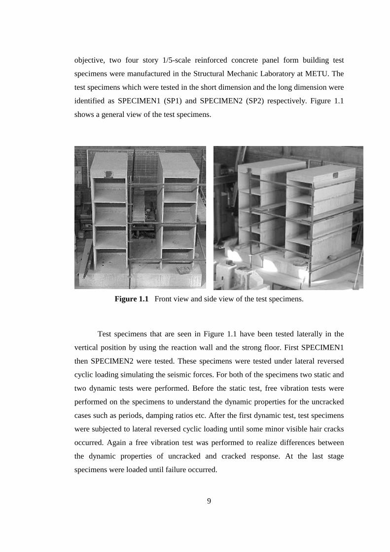
objective, two four story 1/5-scale reinforced concrete panel form building test
specimens were manufactured in the Structural Mechanic Laboratory at METU. The
test specimens which were tested in the short dimension and the long dimension were
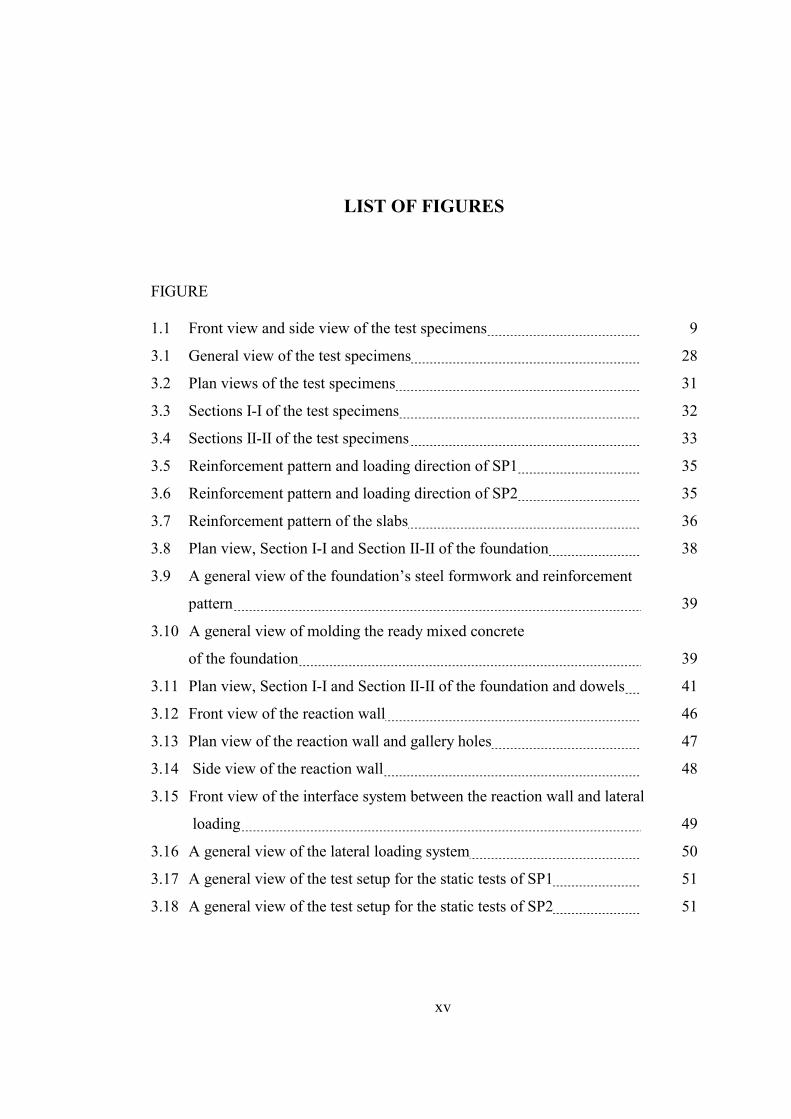
identified as SPECIMEN1 (SP1) and SPECIMEN2 (SP2) respectively. Figure 1.1
shows a general view of the test specimens.
Figure 1.1 Front view and side view of the test specimens.
Test specimens that are seen in Figure 1.1 have been tested laterally in the
vertical position by using the reaction wall and the strong floor. First SPECIMEN1
then SPECIMEN2 were tested. These specimens were tested under lateral reversed
cyclic loading simulating the seismic forces. For both of the specimens two static and
two dynamic tests were performed. Before the static test, free vibration tests were
performed on the specimens to understand the dynamic properties for the uncracked
cases such as periods, damping ratios etc. After the first dynamic test, test specimens
were subjected to lateral reversed cyclic loading until some minor visible hair cracks
occurred. Again a free vibration test was performed to realize differences between
the dynamic properties of uncracked and cracked response. At the last stage
specimens were loaded until failure occurred.
10
CHAPTER 2
LITERATURE SURVEY
To augment the work done in this study, relative to the cyclic loading of 1/5-
scale reinforced concrete panel form buildings, a review of previous experimental
and analytical investigations on shear walls was required. The scope of this chapter,
therefore, deals with a literature review of related work done on the other shear
walls. This investigation will provide information on the behavior of shear walls and
their response to seismic loading conditions.
Paulay and Üzümeri (1975) reported the ductility characteristics of
structural walls. They established a relationship between the curvature and
displacement ductilities of walls with different wall lengths to aspect ratios. The
range of required curvature ductilities for each aspect ratio and displacement ductility
is derived from upper and lower estimate of plastic hinge length. The plastic hinge
lengths are in turn a function of the wall dimensions or aspect ratio. It is understood
that as shear walls become more slender they develop a greater plastic hinge length
resulting in more rotational capacity and in turn greater ductility.
Park and Paulay (1975) contributed significantly to the development of
capacity design procedures and important detailing concept for the design of shear
wall systems. One of the consequences of concern over achieving large ductility led
to the suggestion that the concentrated steel at the ends of the wall should be tied as
columns. Confined concrete at the end of walls would increase the allowable strain in
the compression zone of the wall where strains exceeding 0.004 are required to reach
11
larger curvature ductilities. In addition, more closely spaced ties at the ends of walls
prevent buckling of the concentrated vertical reinforcement.
Paulay (1980) reviewed a shear wall design philosophy for earthquake
resisting shear walls, with emphasis on the desirable energy dissipation and structural
properties. This study was one of the first researches to provide a design philosophy
for shear walls including desirable energy dissipation and potential failure
mechanism. In the light of these findings, it is important to note that ideas about
designing structural walls have changed in the past 25 years.
Paulay, Priestly, and Synge (1982) have investigated the possibilities of
achieving acceptable levels of energy dissipation in squat shear walls, mainly by
flexural yielding of the reinforcement. A review of the possible failure modes was
presented (diagonal tension failure, diagonal compression failure, sliding shear)
along with the methods of prevention. Shear failures originating from diagonal
tension or compression failure, limited ductility and dramatic degradation in strength
and stiffness. For this reason, a more ductile flexural response is desired.
These researchers conducted an experimental program of four squat shear
walls with a height-to-length ratio of 0.5. Two of the specimens had rectangular cross
sections and the remaining included small flanges at the end of a central web wall. A
rigid foundation was used to clamp the specimens to the laboratory floor, and a stiff
top slab ensured an even distribution of the imposed displacements to the wall. The
following observations, based on the experimental findings, were reported:
1. It is possible to ensure a predominantly flexural response, involving considerable
yielding of the flexural reinforcement, for squat shear walls subjected to seismic
loading.
2. Suppression of shear failure by diagonal tension or compression is a prerequisite
for a flexural response and hence, significant energy dissipation.
3. Squat shear walls are likely to fail due to sliding shear along the base unless
specially detailed or subjected to high axial loading. Sliding shear results in the most
significant loss and strength.

12
4. Flanged walls are more seriously affected by sliding shear along interconnecting
flexural cracks.
5. Diagonal reinforcement considerably improves the seismic response of squat shear
walls.
6. The severity of sliding shear increases with increased ductility demand, with
decreasing vertical reinforcement, and with a decrease of the flexural compression
zone.
Cardenas, Hanson, Corley and Hognestad (1982) had an experimental
research on the subject of strength of shear walls for high-rise and low-rise buildings.
Six high-rise and seven low-rise shear walls were tested under combinations of
lateral and axial loads at the laboratories of the Portland Cement Association.
Variables were amount and distribution of vertical reinforcement and effect of
moment to shear ratio. Test results indicated that flexural strength of rectangular
shear walls could be calculated using the same assumptions as for reinforced
concrete beams. Besides, the strength of high-rise shear walls containing minimum
horizontal shear reinforcement was generally controlled by flexure. The results
showed that both horizontal and vertical reinforcement contributed to the shear
strength in low-rise shear walls. The background and development of Section 11.16,
Special Provisions for Walls, of the ACI Building Code (ACI 318-71) were
discussed. They also concluded that the shear strength of low-rise shear walls could
be satisfactorily predicted by ACI-318-71 section 11.16, special provision for shear
walls.
Tegos and Penelis (1988) have made an experimental investigation to study
the behavior of short column and coupling beams reinforced with inclined bars under
seismic conditions. A simple technique to prevent these elements from falling in
premature splitting shear is tested for the first time. According to this technique, the
main reinforcements are arranged at an inclination such as to form a rhombic truss.
Test results show that inclined arrangements is one of the most effective ways to

13
improve the seismic resistance of reinforced concrete low slenderness structural
elements.
Wood (1989) investigated the results of 37 lateral load tests on structural
walls. Lightly reinforced walls with low axial stresses are found to be vulnerable to
failure caused by fracture of the main reinforcement. This mode of failure is of
concern for the design of walls to resist seismic loads because some of the test
specimens failed at overall drift ratios less than 2 percent. Based on the observed
crack patterns on the structural walls, failure modes have been categorized as flexural
failures and shear failures. The shear stress index was used to distinguish between
shear and flexural modes. In more than one-half of the specimens that failed in
flexure, reinforcing bars fractured, however, reinforcing bars fractured in none of the
walls that failed in shear. Failures caused by fracture of the reinforcement were
observed in walls with flexural-stress ratios less than 15 percent. Among the flexural
failures, steel strain was used to identify the walls that were susceptible to fracture of
the main reinforcement. The calculated steel strain in the extreme layer of
reinforcement at the nominal flexural capacity of cross section was used. Fractured
reinforcement was observed in test specimens that were not susceptible to shear
failures and for which the calculated steel strains in the extreme layer of
reinforcement exceeded 4 percent at the nominal flexural capacity. The two walls
which had lowest longitudinal reinforcement ratios (ρ = 0.0027 and ρ=0.0031) failed
by fracture of the tension reinforcement before crushing of the concrete. Except for
these two walls, a flexural hinge developed in the other flexural failures. Walls with
total longitudinal reinforcement ratios less than 1 percent were identified as being
susceptible to fracture of the tensile reinforcement.
Lefas, Kostovos, and Ambraseys (1990) provide a means of understanding
the behavior of shear walls. Their research began with a look into the strength,
deformation characteristics, and failure mechanisms of reinforced concrete structural
walls. Experimental work at Imperial College, England, was carried out on thirteen
isolated cantilever reinforced concrete walls of aspect ratio of one, which were
14
750 mm wide × 750 mm high × 70 mm thick and aspect ratio two, which were
650 mm wide × 1300 mm high × 65 mm thick with a scale of 1:2.5. In all cases, the
walls were monotonically connected to an upper and lower beam. The upper beam
was 1150 mm long × 150 mm deep × 200 mm thick. The lower beam was essentially
the same, except it was 300 mm deep. The upper beam functioned as an element
through which the axial and horizontal loads were applied to the walls and as a case
for the anchorage of the vertical bars and a lower beam was used to clamp the
specimens to the laboratory floor, providing a rigid foundation. The vertical and
horizontal reinforcement comprised high tensile deformed steel bars of 8 mm
(fsy=470 Mpa and fsu=565 Mpa) and 6.25 mm (fsy=520 Mpa and fsu=610 Mpa)
diameter, respectively. Additional horizontal reinforcement in the form of stirrups
confined the wall edges. Mild steel bars of 4 mm (fsy=420 Mpa and fsu=490 Mpa)
diameter were used for this purpose.
The effect of parameters such as the height-to-width ratio, the axial load
level, the concrete strength, and the amount of web horizontal reinforcement on wall
behavior were investigated during those tests. Wall models were tested with load
control under the combined action of a constant axial and horizontal loading
monotonically, increasing up to failure using the test rig. The tests were performed
for three levels of axial load corresponding to 0.0, 0.1, and 0.2 of the uniaxial
compressive strength of the wall cross section that is equal to 0.85×fc×bw×h. The
researchers were able to draw some important conclusions:
1. It was observed that both vertical and horizontal displacements decrease as the
axial load level increases, which also causes an increase in the horizontal load-
carrying capacity and secant stiffness characteristics. This increment becomes more
visible for high height-to-width ratios.
2. Uniaxial concrete strength characteristics within a range of 30 to 55 MPa do not
affect the strength and deformation characteristics of the wall.
3. No significant effect of the horizontal web reinforcement was observed on shear
capacity, which is in contrast to the expected case. Even the amount of horizontal
web reinforcement used is half of the values specified by building codes; the failure
load was not affected.
15
4. Decreasing the height to width ratio and increasing the axial load level extend the
failure region. Failure of the walls occurred due to nearly vertical splitting of the
compressive zone in the tip of the inclined (TYPE I) or the deepest flexural
(TYPE II) crack, followed by splitting of the whole compressive zone.
5. Shear resistance is related with triaxial compressive stress conditions in
compression zone of the base of the wall where flexural moment reaches its
maximum value rather than the strength of the tensile zone of this section.
6. The failure region was more extensive by decreasing height-to-width ratio and
increasing axial load.
Wood (1990) reviewed the results of 143 laboratory tests of low-rise walls to
identify the sensitivity of the measured shear strength to experimental parameters,
such as the loading history and the amount of web reinforcement. The nominal shear
strength of reinforced concrete walls designed to resist seismic loads is defined in
Appendix A of ACI 318-83 to be essentially the same as the nominal shear strength
of reinforced concrete beams that are designed to resist gravity loads. Two quantities
are used to define the nominal shear strength of both types of members, one
attributed to the contribution of the web reinforcement and the other to the
contribution of the concrete. This procedure has been defined as the modified truss
analogy. The applicability of the modified truss analogy for low-rise structural walls
subjected to earthquake-induced load has been questioned in discussions of the ACI
Building Code and is evaluated in this paper. Procedures defined in Appendix A of
ACI 318-83 were found to underestimate the strength of walls with more than 1.5
times the minimum web reinforcement ratio. A reasonable lower bound to the
average shear stress resisted by the test specimens with distributed web
reinforcement in orthogonal directions was (fc')1/2/2 MPa. The maximum average
shear stress tended to increase with an increase in the amount of vertical
reinforcement (longitudinal reinforcement in the boundary elements and vertical web
reinforcement). The increase in shear strength attributed to the vertical reinforcement
was approximated using a shear friction model. An upper limit of 5 × (fc')1/2 / 3 MPa
for the nominal shear strength was also established. A reasonable lower bound to the

16
shear strength of low-rise walls with minimum web reinforcement was found to be
(fc')1/2/2 MPa. The shear strength of the walls was observed to increase with an
increase in the amount of vertical reinforcement in the web and boundary elements.
A shear friction model was used to evaluate the shear strength provided by the
vertical reinforcement.
Wood et al (1991) indicate that the El Faro building failed after the fracturing
of the reinforcement in a first-story wall. The failure of El Faro provides convincing
field evidence that brittleness of reinforced concrete members caused by under-
reinforcement cannot be ignored when designing for earthquake resistance. El Faro
building had extremely heavy structural damage during the Chile Earthquake in
1985, which provides an example of rare, documented failure of a structural wall
system. It was an eight-story apartment building in Vina Del Mar in Chile which had
equal wall area in orthogonal directions but the walls were not uniformly distributed
around the perimeter. Large windows were located along the most damaged sides of
the building. A large crack occurred in structural wall at the first story on this side.
The wall separated along this crack and the portion of the building above the crack
fell to the ground outside the lower portion. A series of linear and limit analyses were
done by Sharon L. Wood in this paper to investigate the cause of the collapse of
El Faro Building. Studies documented in this paper indicate that the building failed
after longitudinal reinforcement fractured in a first-story wall. The calculated
response of El Faro building was compared with that of four other buildings (Villa
Real, Festival, Miramar, Sol) that survived the 1985 Chile Earthquake with light to
moderate damage in Vina Del Mar.
Sharon L. Wood et al compared periods, base-shear strengths and mean drift
ratios for these five buildings. The results indicate that the cause of the severe
damage could not be due to the strength and stiffness characteristics because these
characteristics are not comparable in all the five buildings. As a result it is
understood that the main cause of the collapse was due to structural detail. From the
moment curvature relationship the tensile strains in the boundary reinforcement
exceed two times measured fractured strain of the reinforcement for a compressive

17
strain of 0.003 in the concrete. The magnitude of the calculated strains indicates the
possibility of rupture of reinforcement. The building collapsed after the longitudinal
reinforcement fractured in a first story wall in structural wall system. Fracture
susceptibility in the critical wall was exacerbated by the torsional response of the
building. This paper indicates that lightly reinforced concrete structural walls are
susceptible to brittle mode of failure due to fracture of the reinforcement.
Subedi (1991) proposed a method of analysis for reinforced concrete
coupling beams that is component of coupled shear walls. This study is based on the
subject of reinforced concrete coupled shear wall structures. First, some analyses are
carried on coupling beams. Here, the behavior of coupling beams in the shear mode
failure, known as diagonal splitting, is represented by a mathematical model, and a
method for the ultimate strength analysis is presented. The proposed method of
analysis for RC coupling beams is used to verify the results of nine beams tested by
Thomas Paulay. Second, the ultimate strength calculations or reinforced concrete
coupled shear walls are presented. Three modes of failure of reinforced concrete
coupled shear wall structures, observed in micro-concrete models of 15 story
structures were described. The method is proposed to predict the mode of failure and
the ultimate strength of coupled shear wall structures. The method is based on the
evaluation of the strengths of the coupling beams and the walls at the failure. Two
lateral load cases have been considered: a point load at the top and a four-point
equivalent triangular distribution. The proposed analysis and the test results are
compared.
Pantazopoulou and Imran (1992) investigated the parameters that affect
connection stiffness and shear resistance using experimental evidence and simple
mechanical models. They found that for low reinforcement ratios such as those
frequently used in designing slabs, the existing requirements for walls and
diaphragms may overestimate the nominal shear resistance of connections by as
much as 100 percent. The experimental evidence suggests that gravity loads and a
cyclic load history further reduce the nominal resistance. They derived alternative

18
design equations in this study using a plain-stress approach. They also showed that
the results obtained for a range of reinforcement ratios corroborate the experimental
findings.
Paulay and Priestley (1992) presented brief information about structural
walls. Considerations of seismic design, which address mainly cantilever walls, were
given. Common failure modes encountered in cantilever walls were also described.
They also explain strategy in the positioning of walls, the establishment of a
hierarchy in the development of strengths to ensure that brittle failure will not occur
and preferred mode of energy dissipation in a predictable region.
Pilakoutas and Elnashai (1993) identified some of the common mistakes
that could occur during the testing of reinforced concrete panels and gave an estimate
of the errors involved. Furthermore, the success of such experimental work depends
both on accurate representation of the intended boundary conditions, and the prudent
interpretation of the testing results. A method that decomposes the shear and flexural
components of deformation was given and the differences with other approaches
were shown. From the preceding errors, the following conclusions were drawn:
Forces, which are developed from the connection between loading jack and test
specimen, may result in misleading conclusions. Load-controlled testing under
monotonic loading is of limited use in drawing conclusions pertinent to seismic
design. The method of calculating shear deformation in reinforced concrete panels
should be carefully implemented to avoid large errors.
Paulay and Priestly (1993) carried out experimental and analytical studies
on out-of-plane buckling of rectangular structural walls under severe earthquake
loading. Wall stability becomes a concern when thin wall sections are subjected to
high compressive strains, which could possibly lead to out-of-plane buckling. It is
explained that this concern is based on concepts of Eulerian buckling of struts. An
analytical approach was developed on the minimum required thickness in the vicinity
of the flexural compression zones of ductile structural walls. This prevents the
19
occurrence of out-of-plane buckling in the potential plastic region before the
maximum estimated ductility is developed. The resulting solution of reducing the
occurrence of instability was to limit the wall thickness, bw, to about one-tenth the
height of the wall in the first story. This research shows that out-of plane buckling of
thin walls is more dependent on high inelastic tensile strains in the tensile steel. It is
believed that upon initial moment reversal, all compressive stresses will be resisted
by the steel because the cracks formed in the concrete due to the previous tensile
cycle will not have completely been closed. The result may be flexural compressive
force that does not coincide with the center of the wall thickness, bw. This
eccentricity together with small-dislocated concrete particles and unaligned crack
surfaces could lead to instability. It was founded that the properties of inelastic
buckling are mainly affected by wall length and previously experienced tensile strain
rather than excessive compression strain.
Fintel (1993) presented a condensed report on the philosophy underlying the
design for earthquake resistance of multi-story structures in reinforced concrete. The
criteria for earthquake performance were discussed and behavior of structures under
earthquake excitation was explained briefly. He noted that the evolution of
earthquake engineering of buildings started in the 1950’s when the ductile moment
resistant frame was introduced. Most research during that period emphasized the
importance of a ductile moment resisting frame to reduce seismic forces. Shear walls
were expected to suffer severe damage stemming from their brittle response due to
the fact that rigid structures attract higher seismic forces. It was concluded that
severe damage could be expected in shear walls due to brittle response of the shear
walls to in plane lateral forces. Based on this thinking, shear walls were considered
undesirable for earthquake resistance, and buildings were built with moment
resistance frames. However, recorded observations of severe earthquakes (e.g.,
Yugoslavia, 1963, Venezuela, 1967, California, 1971, Nicaragua, 1972, Romania,
1977, Mexico, 1985, Chile, 1985, and Armenia, 1988) over the past thirty years have
shown otherwise. During these earthquakes, hundreds of concrete structures, based
on moment resistant frames, collapsed due to excessive interstory distortions that
20
caused failures of columns. However, buildings containing shear walls exhibited
extremely good earthquake performance.
Many engineers confused ductility with flexibility (flexibility with ductility))
in the early days of seismic design, and as a result, a large number of buildings were
built in a flexible manner. These structures were prone to large interstory drift
leading to structural failure. The shear walls, on the other hand, were capable of
resisting the interstory drift distortions associated with the seismic events noted
above.
Incorporating shear walls to resist seismic actions requires the engineer to
become aware of the potential failure mechanisms, and to control some of the
undesired characteristics. An earthquake-resisting shear wall structure should ensure
survival during the largest ground shaking that can be expected. It should also protect
components of a building against all but superficial damage during more frequent
disturbances of smaller intensity. Proper detailing will ensure structural survival
through energy dissipation by hysteretic damping. Today shear walls are at the
forefront for the earthquake resisting elements, and research has also tried to provide
a degree of ductility.
Pilakoutas and Elnashai (1995) set out an experimental program to quantify
the true ductility and energy absorption of reinforced concrete walls. Another series
of wall tests commonly used to corroborate analytical models are the shear wall
series tested by Pilakatus and Elnashai. Six isolated cantilever concrete walls, which
have aspect ratio of 2 and scale 1:2.5, were tested under severe cyclic loading up to
failure. The horizontal load was applied through the top beam, designed to spread the
load over the wall panel. Displacements were imposed along the top slab in
increments of 2 mm, consisting of two full cycles per displacement level. The cyclic
loading was provided by displacement control, at a very slow rate. The
displacements were incremented at 2-mm intervals with two full cycles at each
displacement level.
Walls were designed in three pairs; each pair having equal flexural
reinforcement but different shear reinforcement. Concentrated reinforcement in the
21
boundary elements was used to maximize the flexural capacity, and the web
reinforcement was kept nominal. Different amounts of shear reinforcement were
used in each pair of walls to investigate the effect of various degrees of safety
margins in shear. The shear reinforcement in the web walls was varied to investigate
the effect of various degrees of safety margins in shear. The confinement of the
boundary elements varied as a consequence of the variation in the shear
reinforcement. As a result, the amount of confinement of the boundary region was
also varied.
They found that the strength and deformational characteristics of specimens
were not affected significantly by shear reinforcement in excess of the amount
required to resist the maximum applied load. Concrete dilatation causes the extension
of the wall in both the longitudinal and lateral direction. Considerable amount of
extension of the wall in the vertical direction occurred due to excessive strains at the
plastic hinge region. Shear force is carried by both the concrete in compression and
the link reinforcement. Failure took place after the link reinforcement yielded and
when the shear resistance of the concrete in compression was exceeded.
The researchers reported some of the following observations:
1. Failure mode depended mainly on the amount and distribution of the shear
reinforcement.
2. The strength and deformational characteristics of the specimens were not affected
significantly by the shear reinforcement in excess of the amount required to resist the
maximum applied load.
3. Shear force was partly transmitted by the concrete in compression and partly by
the horizontal (link) reinforcement that enables shear stresses to be resisted through
the concrete in the tensile zone. Failure occurred after yielding of the links, and when
the shear resistance of concrete in compression was exceeded.
4. Concrete dilatation following cracking caused the extension of the wall in both the
longitudinal and lateral directions.
5. Significant extension of the wall in the vertical direction took place following
yield due to the accumulation of irrecoverable strains mainly within the plastic hinge
zone.
22
Pilakoutas and Elnashai (1995) evaluated the results that are presented in
the companion paper “Cyclic Behavior of Reinforced Concrete Cantilever Walls,
Part I: Experimental Results.” Evaluation of these results and comparisons with
analytical predictions are made in this paper. Analytical techniques employed vary
from linear elastic to nonlinear section analysis. In the first section of this paper, the
stiffness characteristics were investigated, since this is the one of the most important
parameters in earthquake-resistant code-based design. In the second section, the limit
states of first yield and ultimate moments were investigated because of their
significance in determining the actual capacity and ductility of members. Finally, the
ductility and energy-dissipation aspects of the behavior were presented and
discussed.
Aktan and Bertero (1995) evaluated the provisions of 1982 UBC,
ACI 318-83, and ATC 3-06 pertaining to seismic shear design of slender walls in
mid-rise construction. In the event of major ground shaking in regions of high
seismic risk, the actual shear strength demand is expected to equal that associated
with the axial-flexural supply. Thus, the codes minimum design requirements ought
to insure that flexure, and not shear, will control the seismic response during the
expected rare, major seismic event. The codes do not implement this condition.
Expressions suggested by design documents for computing the shear strength of
walls were evaluated by comparing the predicted and measured strengths of 10 wall
specimens tested at Berkley. Although generally conservative, since code
expressions do not incorporate the actual shear resisting mechanisms of walls under
seismic effects, it is possible for the expressions to mislead the designer to poor shear
design. Recommendations are formulated to improve the current shear design
procedures by: (1) Relating the shear strength demands to the actual axial-flexural
supply, and (2) Incorporating the actual shear resisting mechanisms in predicting
shear strength supply of walls.
Sittipunt and Wood (1995) developed a procedure to assist the designer in
evaluating the cyclic response of structural walls and identifying walls that are
susceptible to undesirable modes of failure. Reinforced concrete walls, exposed to
23
seismic loading, experience pinched hysteretic curves and poor energy dissipation
characteristics, experience stiffness degradation with cycling, and may exhibit a
sudden loss in lateral load capacity due to web crushing. The authors have suggested
that these issues need to be considered in the design process and controlled by the
use of diagonal reinforcement in the web. It has been identified as an efficient means
of limiting shear distortions, increasing energy dissipation, and reducing the
likelihood of shear failures in walls. Thirteen walls tested at the Portland Cement
Association were investigated to illustrate the effect of web reinforcement
arrangement under cyclic loading.
Failure of the specimens occurred by one of two methods: loss of flexural
capacity caused by buckling or fracture of the longitudinal reinforcement, or a loss of
shear capacity due to crushing of the concrete in the either boundary element of the
web. In the current US building codes, the nominal shear strength of slender walls is
assumed to increase in proportion to the amount of web reinforcement. However,
many walls subjected to cyclic loading fail due to web crushing after yielding in
flexure, which is not accounted for in the code. The results of the PCA tests show
that increasing the amount of horizontal web reinforcement has a negligible influence
on the hysteresis response of the walls. To study the influence of web reinforcement,
six walls with varying arrangements were analyzed.
An increase in the horizontal web reinforcement and an increase in the
vertical web reinforcement were not sufficient to improve the cyclic response of
walls or reduce the shear distortion at the base. Anchoring with 0.30% of the web
reinforcement was effective in reducing the average shear strain at the base. The
unanchored bars could not yield at the base, however they were effective in
controlling cracks widths. The increase in shear stiffness is, thus, due to aggregate
interlock. The final two configurations utilized diagonal reinforcement of identical
area. The diagonal reinforcement did not change the strength of the walls
significantly, but the hysteric response was more rounded and the shear stiffness did
not degrade appreciably. This significant improvement occurs because the diagonal
reinforcement runs nearly perpendicular to web cracks. After cracking, most of the
force is carried across the cracks by diagonal reinforcement in direct tension. In walls

24
with only vertical and horizontal reinforcement, the reinforcement is inclined to the
cracks and the force transmitted across the cracks is carried by dowel action. This is
characteristic to stiffness degradation. Therefore, utilizing diagonal reinforcement in
webs subjected to reversed loading conditions provided an improvement in the
response and should be used in the design process.
Tassios, Moretti and Bezas (1996) in their study presented the results of an
experimental program on coupling beams under cyclic loading. They tested ten
specimens with five different reinforcement layouts and two different shear ratios
(which are αs=0.50 and 0.83) with scale 1:2. The effect of various layouts of
reinforcement on the hysteretic response of “short” (αs=0.50) and “medium”
(αs=0.83) coupling beams has been investigated. The performance of the specimens
according to their ductility has been classified. This paper offers quantitative
evidence for the selection of layouts of reinforcement other than the conventional or
bidiagonal ones, depending on the shear ratio of the coupling beams. Moreover, the
stiffness degradation of coupling beams can be evaluated and possibility used for a
more pragmatic estimation of the reduction of bending moments of the main walls.
Grupta and Rangen (1998) tested eight high-strength concrete (HSC)
isolated cantilever structural walls under the combined action of in-plane axial and
horizontal loads. In addition, they presented the analytical studies on the strength of
reinforced concrete structural walls, which also predict the ultimate and failure
modes. Test specimens were one-third scale model, which have overall length of
1000 mm with 75 mm thick and 375×100 mm edge elements. The dimension of the
top beam and the bottom (foundation) beam were selected such that they did not
suffer premature failure and that they were stiffer than the wall. The 28-day concrete
compressive strength of the test specimens was 70 MPa. The maximum size of
aggregate was 7 mm in order to ensure good compaction of concrete in the test
specimens. The test wall specimens were cast horizontally in timber molds. The
specimen dimensions achieved were within 0.5 percent accuracy. Test parameters
investigated were the longitudinal reinforcement ratio, transverse reinforcement
25
ratio, and axial load level. The ultimate loads and failure load obtained by the
analytical study of Grupta and Rangen show good correlation with not only the
results of their studies but also with those available in the literature.
Paulay (1999) reviewed elementary but largely forgotten principles, relevant
to the seismic behavior of structural systems comprising elements with very different
characteristics. In such structures the displacement at the ultimate limit state may be
associated with very different displacement ductility demands imposed on
constituent elements. He showed how, by simulating nonlinear ductile structural
response with bilinear modeling, the unavoidable restriction on the system ductility
capacity, necessary to protect elements with the smallest displacement potential, can
be readily determined. To illustrate the applications of fundamental principles a few
simple examples are presented. The exploitation of the principles presented in
structures with restricted ductility and very different plastic mechanisms is
illustrated.
Balkaya and Kalkan (2002) investigated the applicability and accuracy of
inelastic pushover analysis in predicting the seismic response of tunnel form building
structures. The contribution of transverse walls and slab-wall interaction during the
3D action, the effects of 3D and 2D modeling on the capacity-demand relation, as
well as diagram flexibility, torsion and damping effects were investigated. Two
different buildings having similar plan and sections with different story levels were
analyzed by utilizing the 3D and 2D finite element models with the use of the
developed isoparametric shell element. This paper also makes comparisons between
the conventional 2D solutions and the applied 3D analyses of presented case studies
and illuminates the reasons for their differences. In general, total resistance capacities
of the three dimensionally analyzed structures were observed to be more than that of
two dimensionally modeled cases. This study showed that the applied methodology
has a considerable significance for predicting the actual capacity, failure mechanism,
and evaluation of the seismic response of tunnel form buildings.
26
Balkaya and Kalkan (2003) investigated the consistency of empirical
equations in current seismic code provisions related to dynamic properties of shear-
wall dominant buildings constructed by using tunnel form techniques. For that
reason, a total of 80 different building configurations were analyzed by using three-
dimensional finite-element modeling and a set of new empirical equations was
proposed. It is demonstrated that current earthquake codes overestimate the
performed finite-element analysis results for rectangular plans and most of the time
underestimate them for square plans. The recommended empirical equations are
presented in detail in this paper and are considered to be appropriate for the
estimation of the period of tunnel form building structures for 2-15 story levels with
various architectural configurations. The results of the analyses demonstrated that
given formulas including new parameters provide accurate predictions for the broad
range of different architectural configurations, roof heights and shear-wall
distributions, and may be used as an efficient tool for the implicit design of these
structures.
27
CHAPTER 3
TEST SPECIMENS AND EXPERIMENTAL TECHNIQUE
3.1 GENERAL
This chapter contains details pertaining to the test specimens. It includes the
design of panel form test specimens, the construction process, the properties of the
materials used, description of the test setup, loading system and the testing facility. It
also includes instrumentation utilized during the test and test procedure.
The main objective of the research reported in this thesis is to study the
behavior of panel form structures under seismic action. Since system testing is
expensive and time-consuming, test specimens had to be designed and detailed
carefully, construction of the test specimens had to be planned considering all the
details and instrumentation had to be designed considering the main objectives for
this experimental research.
The experimental study conducted by the author was a part of research
program sponsored by National Science and Technical Research Council of Turkey
(TUBİTAK-İNTAG 561).
3.2 TEST SPECIMENS
3.2.1 General
The experimental work described in the following involves the testing of two
four-story 1/5-scale reinforced concrete panel form building test specimens under
lateral reversed cyclic loading, simulating the seismic forces and free vibration tests.
1/5-scale reinforced concrete panel form building test specimens were manufactured
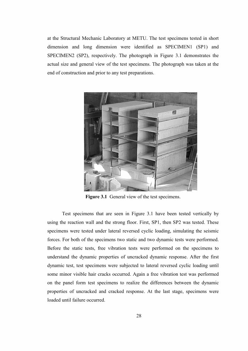
28
at the Structural Mechanic Laboratory at METU. The test specimens tested in short
dimension and long dimension were identified as SPECIMEN1 (SP1) and
SPECIMEN2 (SP2), respectively. The photograph in Figure 3.1 demonstrates the
actual size and general view of the test specimens. The photograph was taken at the
end of construction and prior to any test preparations.
Figure 3.1 General view of the test specimens.
Test specimens that are seen in Figure 3.1 have been tested vertically by
using the reaction wall and the strong floor. First, SP1, then SP2 was tested. These
specimens were tested under lateral reversed cyclic loading, simulating the seismic
forces. For both of the specimens two static and two dynamic tests were performed.
Before the static tests, free vibration tests were performed on the specimens to
understand the dynamic properties of uncracked dynamic response. After the first
dynamic test, test specimens were subjected to lateral reversed cyclic loading until
some minor visible hair cracks occurred. Again a free vibration test was performed
on the panel form test specimens to realize the differences between the dynamic
properties of uncracked and cracked response. At the last stage, specimens were
loaded until failure occurred.
29
3.2.2 Dimensions of the Test Specimens and the Formwork
The experimental work described in the following involves the testing of two
four-story 1/5-scale reinforced concrete panel form building test specimens under
lateral reversed cyclic loading, simulating the seismic forces and free vibration tests.
SP1 was tested along short dimension and SP2 was tested along long dimension. All
specimens were cast vertically by using 1/5-scale steel forms. The steel formwork
was manufactured from 2.5 mm thick steel plates. Steel plates were assembled with
bolts, forming the formwork. The 1/5-scale steel forms of the specimens were
manufactured with an error of 1/10 of one millimeter. The forms were stiff enough to
avoid any deformations during the molding process.
The plan view of the test specimens is given in Figure 3.2 (All dimensions
given in this study are in mm). The two sectional drawings, I-I and II-II are given in
Figure 3.3 and Figure 3.4, respectively. Each test specimen has 880×2000 mm plan
dimensions. There was an empty space of 870 mm between two specimens. Both
specimens were manufactured on the same foundation with 2.4 m width, 3.2 m
length and 0.4 m thickness. There was a 200 mm thick slab at the fourth story to
prevent the local deformations while loading the test specimens under reversed cyclic
loading at this level.
The specimens were monolithically connected to the upper extra slabs and the
foundation. The upper slabs also functioned both as the elements through which
horizontal loads were applied to the specimens and as cages for the anchorage of the
vertical bars. The top slabs of the specimens were heavily reinforced with φ8
reinforcing bars. It consisted of top and bottom reinforcement in both directions with
a bar spacing of 100 mm. The ends of the bars had an anchorage length of 100 mm in
the form of a 90-degree bend. This heavy reinforcement in the top slab was required
to ensure stiff slab members so that failure would be concentrated in the wall
members. The clear cover for the reinforcement was 40 mm in the top slab. The self-
weight of the top slab contributed an additional 7.48 kN of axial load.
The foundation was utilized to clamp down the specimens to the laboratory
30
floor, simulating a rigid foundation. Forming the foundation constituted the first
phase of the construction of the panel form test specimens. The second phase of the
construction consisted of casting the walls and slabs of the test specimens. The final
phase of the test specimens included the construction of the top slab. Wall thickness
was 40 mm, slab thickness was 30 mm and story heights were
650 mm. The shear wall consisted of an H beam cross-section. The two flange walls
were 620 mm high × 40 mm thick × 2000 mm long. The web walls were
620 mm high × 40 mm thick × 800 mm long. The ratio of the wall area to the floor
area was 10.91%. Total overall heights of the specimens were 2770 mm.

31
Figure 3.2 Plan views of the test specimens.
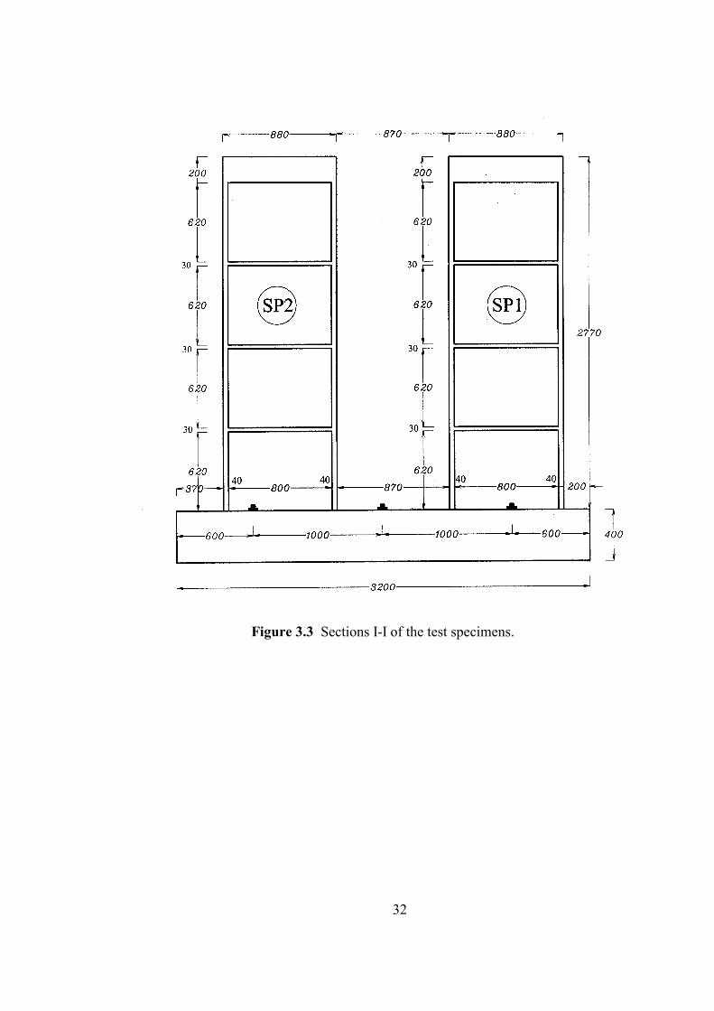
32
Figure 3.3 Sections I-I of the test specimens.
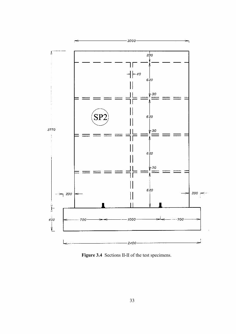
33
Figure 3.4 Sections II-II of the test specimens.

34
3.2.3 Details of the Test Specimens
The dimensions of the test specimens are given in Section 3.1.1. The
dimensions and detailing of the reinforcement are chosen to reflect the common
deficiencies encountered in practice in Turkey. According to AY (1997) the
minimum reinforcement ratio for shear walls is 0.0025. However if the ratios of wall
area to building plan area satisfy some requirements stated in AY (1997), the
minimum reinforcement ratio for shear walls in this situation is ρmin = 0.0015. The
ratios of wall area to building plan area satisfy requirements stated in AY (1997). To
provide minimum reinforcement ratio for shear walls in the vertical and horizontal
directions respectivelyρhmin = ρvmin = 0.0015; 2 mm diameter one-layer mesh
reinforcement was used. The spacing of the wall reinforcement is 50 mm in both
directions. There are 40φ2/50 mm bars in each flange and 17φ2/50 mm bars in the
web in the longitudinal direction of the walls. The longitudinal reinforcement of the
shear walls was spliced at foundation level. 97φ2.5/50 mm dowels cast in the
foundation had a length of 80φ (80×2.5 mm = 320 mm). The longitudinal
reinforcement of the shear walls was spliced at floor level with a splice length of 50φ
(50×2 mm = 100 mm). No splice problem was faced during the experiments at those
locations. In none of the tests bond slip of the reinforcement was evident.
In slabs, 2.5 mm diameter one-layer mesh reinforcement was used. The
spacing of the slab reinforcement was 50 mm in both directions. One-layer mesh
reinforcement was placed in the middle of the slabs. The ends of the bars had an
anchorage length of 50 mm in the form of a 90-degree bend. The reinforcement ratio
for slabs along the long and short dimensions was 0.0025%. Reinforcement patterns
and loading directions of SP1 and SP2 are given in Figure 3.5 and Figure 3.6,
respectively. The reinforcement pattern of the slabs is given in Figure 3.7.
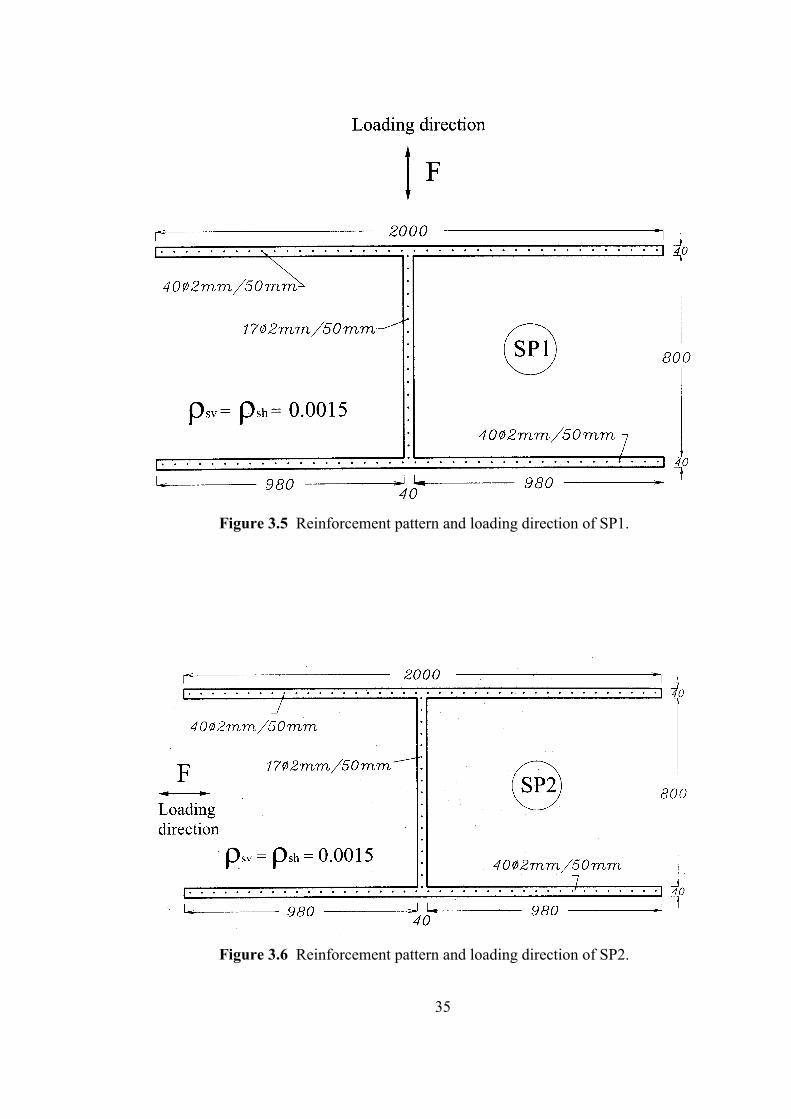
35
Figure 3.5 Reinforcement pattern and loading direction of SP1.
Figure 3.6 Reinforcement pattern and loading direction of SP2.

36
Figure 3.7 Reinforcement pattern of the slabs.

37
3.3 FOUNDATION OF THE TEST SPECIMENS
Forming the foundation constituted the first phase of the construction of the
panel form test specimens. One-meter distance between the holes on the strong floor
led to a design of a big foundation that has a length of 3.2 m, width of 2.4 m, and
thickness of 0.4 m. This foundation enabled to place two 1/5-scale reinforced
concrete panel form buildings on the same foundation. The foundation can be fixed
to the strong floor at six points for SP1 and four points for SP2 by means of 50 mm
diameter and 1.5 m length high strength steel bolts. Plan view, cross section I-I and
cross section II-II of the foundation are given in Figure 3.8.
Steel forms were prepared for molding of the foundation concrete.
Approximately 3m3 of concrete was required for the production of the foundation.
The weight of the foundation was 77 kN. Ready mixed concrete was ordered from a
local ready mix plant company. Before placing the concrete, the cavities inside the
forms were cleaned and greased to facilitate their removal when concrete was set.
A general view of the foundation’s steel formwork and reinforcement pattern are
shown in Figure 3.9. Figure 3.10 shows a general view of molding the ready mixed
concrete of the foundation. Mechanical vibration was used for the compaction of the
concrete. This mechanical vibration was imparted by means of a vibrator, which
operated with the help of an electric motor. Nine cylinder specimens were taken for
the quality control of concrete. At the conclusion of testing, compression cylinder
tests were conducted on standard (150 mm × 300 mm) concrete cylinders batched
from the truck. The cylinders were tested at 28 days at a loading rate of 0.005 mm/s.
The grade of the ordered ready mixed concrete was C25, which should have a
compressive strength of 25 MPa at 28 days. According to the standard cylinder tests,
the concrete of the foundation had a final strength of 44 MPa.

38
Figure 3.8 Plan view, Section I-I and Section II-II of the foundation.

39
Figure 3.9 A general view of the foundation’s steel formwork and reinforcement
pattern.
Figure 3.10 A general view of molding the ready mixed concrete of the foundation.

40
The foundation of the test specimens were heavily reinforced with twenty-
millimeter diameter S420 type deformed bars. In short direction 20φ20/250 mm
deformed bars were used and in long direction 30φ20/220 mm deformed bars were
used. These reinforcements were placed on bottom and top faces of the foundation to
resist the reversed cycling of the testing load. The clear cover for the foundation
reinforcement was 40 mm. This heavy reinforcement causes the reinforcement ratio
for the foundation along the long and short dimensions to be 0.73% and 0.82%,
respectively, which was required to ensure stiff foundation so that premature failure
would not occur in foundation.
An important step was to place the dowels prior to casting. To transmit the
loads of test specimens to the foundation, 2.5 mm diameter mesh reinforcements,
which have 50 mm × 50 mm spacing, were used as dowels. To provide adequate
development length, these dowels were extended into footing 30 mm. They were tied
to the reinforcement of the foundation. They also extended into the walls 200 mm,
that is 100 times that of the wall’s bar diameter (100 ×2.0 mm = 200 mm). Plan view,
Section I-I and Section II-II of the foundation and dowels are given in Figure 3.11.

41
Figure 3.11 Plan view, Section I-I and Section II-II of the foundation and dowels.
3.4 MATERIALS
Reinforced concrete panel form specimens were cast monolithically in the
vertical direction. The concrete of the 1/5-scale reinforced concrete panel form
specimens was produced at the structural Mechanics Laboratory of METU. A
concrete mixture with a maximum aggregate size of 7 mm and cement content of
about 436 kg/m3 were used in the panel form test specimens. According to Turkish
Seismic Code (AY-1997) in high seismic zones minimum C20 must be used. The

42
average 28 days characteristic cylinder strength of concrete must be more than
200 kg/cm2. The target compressive cylinder strength of the 1/5-scale reinforced
concrete panel form specimens was more than 20 MPa. The concrete mix for the
walls required a special order that would provide an increased flow of the concrete so
that it would penetrate through the thin wall members. Prior to casting,
superplasticizer (sikament300) was added to bring the slump up to 200 mm. The
superplasticizer improved the floor of the concrete while improving the strength and
hardening time of the concrete. Table 3.1 gives the mixture proportions of concrete
for the 1/5-scale reinforced concrete panel form specimens. Materials used in the
mixture are given by weight for 1 m3 concrete. The cylinders from the panel form
test specimens were tested on the day of testing. At the test day of SP1 and SP2, the
strength of concrete was 35 MPa.
Special attention was given to curing. Curing was done by covering the
specimens with wet burlap which kept the concrete moist and as near as possible to
the ideal temperature for chemical hydration.
At least nine standard cylinder test specimens were taken from each batch in
order to determine the concrete strength. The test cylinders were 150 mm in diameter
and 300 mm in height. The test cylinders were kept under the same moist curing
conditions as the test specimens. Each time, three cylinders were tested to obtain the
average strength of concrete.
Table 3.1 Mix design of the panel form specimen (weight for 1 m3 of concrete).
Weight (kg) Proportions by weight (%)
Cement 436 19.05
0-3 mm Aggregate 864 37.75
3-7 mm Aggregate 745 32.55
Water 240 10.48
Sikament 300 4 0.17
Total 2289 100.00
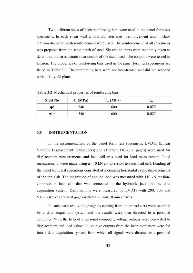
43
Two different sizes of plain reinforcing bars were used in the panel form test
specimens. In each shear wall 2 mm diameter mesh reinforcement and in slabs
2.5 mm diameter mesh reinforcement were used. The reinforcement of all specimens
was prepared from the same batch of steel. Six test coupons were randomly taken to
determine the stress-strain relationship of the steel used. The coupons were tested in
tension. The properties of reinforcing bars used in the panel form test specimens are
listed in Table 3.2. The reinforcing bars were not heat-treated and did not respond
with a flat yield plateau.
Table 3.2 Mechanical properties of reinforcing bars.
Steel No fsy(MPa) fsu (MPa) εsu
φφφφ2 540 600 0.025
φφφφ2.5 540 600 0.025
3.5 INSTRUMENTATION
In the instrumentation of the panel form test specimens, LVDTs (Linear
Variable Displacement Transducers) and electrical DG (dial gages) were used for
displacement measurements and load cell was used for load measurement. Load
measurements were made using a 110 kN compression-tension load cell. Loading of
the panel form test specimens consisted of increasing horizontal cyclic displacements
of the top slab. The magnitude of applied load was measured with 110 kN tension-
compression load cell that was connected to the hydraulic jack and the data
acquisition system. Deformations were measured by LVDTs with 200, 100 and
50 mm strokes and dial gages with 50, 20 and 10 mm strokes.
In each static test, voltage signals coming from the transducers were recorded
by a data acquisition system and the results were then directed to a personal
computer. With the help of a personal computer, voltage outputs were converted to
displacement and load values i.e. voltage outputs from the instrumentation were fed
into a data acquisition system, from which all signals were directed to a personal

44
computer. A computer program written at METU stored the data as force and
displacement. This program also monitored the data as numbers and graphics on the
screen.
In all tests in this study, the displacement of each story was measured with
respect to the foundation. These readings would be used to construct load-
displacement and load-inter-story drift curves. The lateral displacements of the test
specimens at each floor level were measured by means of displacement transducers.
Shear deformations were measured on both the first and the second story walls in the
static tests of SP1. Shear deformations were measured on the first story walls in the
static tests of SP2. In the specimens, average shear deformations of the wall panels
were measured by means of diagonally placed displacement transducers. Transducers
were located 100 mm away from the corner of the walls. The reason for choosing
this location was to avoid localized effects like crushing of concrete during the
experiment. Strains were measured on both faces of the walls at the base, which
would enable the calculation of the curvature.
The rigid body rotations and displacement of the foundation and reaction wall
were measured by means of mechanical dial gages in all tests. Two gages in
horizontal direction, two gages in lateral direction and two gages in vertical direction
were mounted on the foundation and reaction wall. These gages were monitored
manually. The readings were acquired at the end of each cycle. In all tests no
appreciable movement was observed in these dial gages (∆≈1/50mm), which meant
that in the load range applied during the test, no appreciable movement occurred
either at the foundation or at the reaction wall in all tests. Moreover, all
measurements on the test specimens were taken relative to the foundation. Therefore,
rigid body movements would not affect the readings of the test specimens.

45
3.6 TEST SETUP AND LOADING SYSTEM
The testing apparatus required for the reversed cyclic loading of the panel
form test specimens is explained in detail in this section. The testing system
consisted of the strong floor, reaction wall, loading equipment, instrumentation and
the data acquisition system.
The Structural Mechanics Laboratory of METU has a strong floor for fixing
the test specimens to the test floor. This floor has a thickness of 600 mm.
Additionally a working drift (gallery) lies under the strong floor that enables to work
under the floor easily. Holes are left on the floor, which allow fixing of the test
specimens to the floor. Totally, 48 holes are lined up as two rows with 1-meter
spacing. The distance between the rows is also 1 meter. The diameter of these holes
is 150 mm.
The foundation of the test specimen was fixed to the strong floor by means of
specially produced high strength steel bolts (Dywidag). These bolts had a diameter of
50 mm. 6 and 4 holes were used to fasten the footing to the strong floor for testing
the SP1 and SP2, respectively. The footing had to be anchored with a uniform force
to the floor. To accomplish this, a pre-tensioning system was built from steel
sections. First, all Dywidags were tensioned with this system up to 120 kN. Then, the
bolts were tightened at their stretched position. After bolting, the tension force was
released from the Dywidags. All the Dywidags were tightened almost by the same
amount of force in this way.
To make vertical testing of the specimens’ possible, there was a need for a
reaction wall that provides lateral loading. In the laboratory, a reaction wall was
fixed to the strong floor by means of totally 8 Dywidags. The total height of the
reaction wall was 4.58 m. There are totally 14 holes on the wall that are spaced at
two columns and seven rows. These holes match correctly the holes on the floor; in
other words, the distance between two columns is 1 m. Also, the length between the
rows is 610 mm. Front view, top view and side view of the reaction wall are given in
Figure 3.12, Figure 3.13and Figure 3.14, respectively.
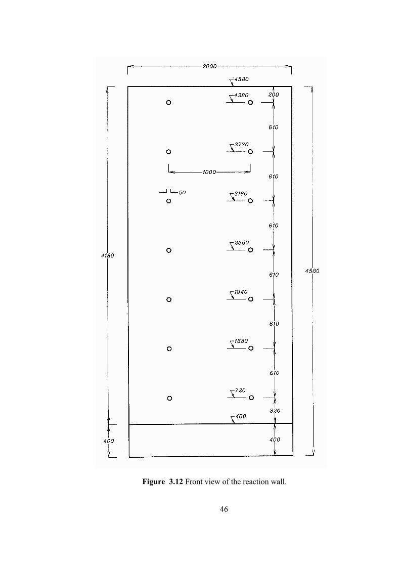
46
Figure 3.12 Front view of the reaction wall.
47
Figure 3.13 Plan view of the reaction wall and gallery holes.
48
Figure 3.14 Side view of the reaction wall.
The lateral loading system had to be fixed perpendicularly to the reaction
wall and the extra slab of the test specimen. This loading system consisted of hinges
at the ends, a load cell and a hydraulic jack (cylinder). This loading system had to
enable the loading jack to come exactly to the center-point of the fourth story slab.
Therefore, this system had to be freely moveable on the reaction wall allowing
accurate positioning. For this reason, a rail system was designed using heavy steel
sections. Photographs of the front view and side view of the interface system
49
between the reaction wall and lateral loading are given in Figures 3.15 and 3.16,
respectively. The top and bottom part of the system consisted of build-up box
sections welded to two U200 steel sections. To enable sliding, two U140 steel
sections were put together with a space in between. The width of this space was
40 mm. U140 steel sections were strengthened by welding 6×1 mm steel plates to the
flanges. The sliding system was welded to the top and bottom heads to form the left
and right columns. These columns enable sliding up and down directions. In order to
allow movement in horizontal direction, the same sliding mechanism was placed on
the steel columns. A 400×400 mm steel plate with a thickness of 30 mm was
attached on this mechanism. This plate allowed fixing the hinge of the lateral loading
system.
Figure 3.15 Front view of the interface system between the reaction wall and lateral
loading.
50
Figure 3.16 A general view of the lateral loading system.
The lateral load was applied at the fourth story floor level through a hydraulic
jack. Before molding of the concrete of the extra slab on the fourth story, a steel plate
was placed at the face of the exterior joint. This steel plate was welded to the
longitudinal lateral reinforcement of the extra slab to transmit the lateral load from
the hydraulic jack safely during the cyclic loading. A load cell was connected in front
of the hydraulic jack in order to measure the magnitude of the applied lateral load. A
steel stiffened pipe was put between the load cell and test specimens to fill the gap
between the reaction wall and the test specimens. This pipe was welded to the steel
plate at the joint. At both ends of this loading system, hinges were placed to ensure
axial load application. A general view of the loading system is given in Figure 3.16.
A general view of the test setup, loading system, instrumentation, reaction
wall and data acquisition system for static test of SP1 and SP2 are shown in Figure
3.17 and Figure 3.18, respectively.
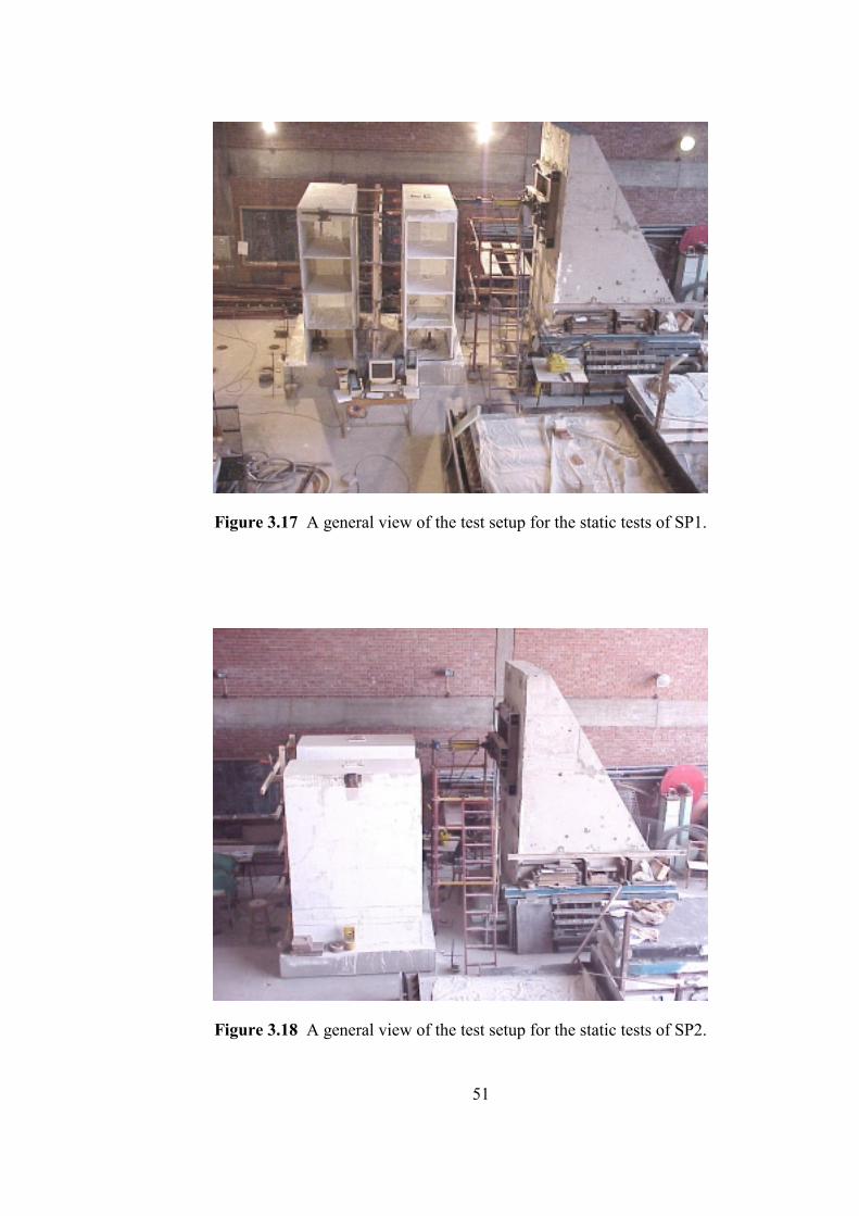
51
Figure 3.17 A general view of the test setup for the static tests of SP1.
Figure 3.18 A general view of the test setup for the static tests of SP2.
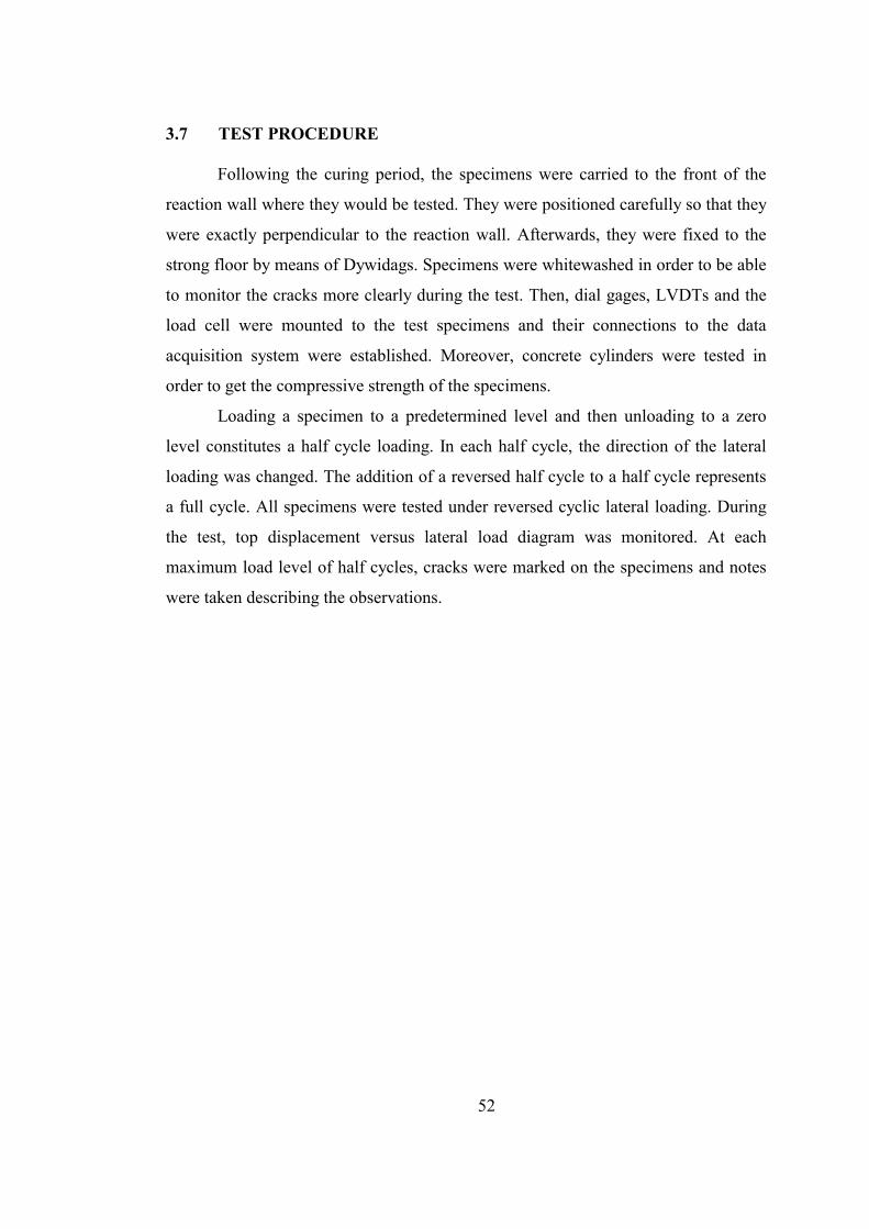
52
3.7 TEST PROCEDURE
Following the curing period, the specimens were carried to the front of the
reaction wall where they would be tested. They were positioned carefully so that they
were exactly perpendicular to the reaction wall. Afterwards, they were fixed to the
strong floor by means of Dywidags. Specimens were whitewashed in order to be able
to monitor the cracks more clearly during the test. Then, dial gages, LVDTs and the
load cell were mounted to the test specimens and their connections to the data
acquisition system were established. Moreover, concrete cylinders were tested in
order to get the compressive strength of the specimens.
Loading a specimen to a predetermined level and then unloading to a zero
level constitutes a half cycle loading. In each half cycle, the direction of the lateral
loading was changed. The addition of a reversed half cycle to a half cycle represents
a full cycle. All specimens were tested under reversed cyclic lateral loading. During
the test, top displacement versus lateral load diagram was monitored. At each
maximum load level of half cycles, cracks were marked on the specimens and notes
were taken describing the observations.

53
CHAPTER 4 TEST RESULTS AND OBSERVED BEHAVIOR OF SPECIMEN1
4.1 INTRODUCTION
This chapter summarizes the instrumentation on SP1 for the first and second
static tests, qualitative and quantitative experimental results and behavior of the
panel form test specimen, SP1. The quantitative results will include lateral
displacement curves of each story, story drift ratios with the applied lateral force,
shear deformation and moment curvature curves. The qualitative results will be
presented in the form of photographs of the SP1 taken during testing, displaying the
crack patterns, cracking and/or crushing locations, and the state of the SP1 at failure.
In the instrumentation of the SP1 for the static tests LVDTs (Linear Variable
Displacement Transducer), electronic and mechanical dial gages were used for
displacement measurements and load cell was used for load measurements. Load
measurements were done using a 110 kN compression-tension load cell.
4.2 STATIC TEST ON UNDAMAGED SPECIMEN1
After the free vibration test was done on the undamaged SP1, the reversed
cyclic static test was applied. The aim of this test was to investigate the behavior of
the SP1 up to cracking.
In the first static test, lateral deformations were measured by dial gages with a
20 mm strokes at the fourth story and dial gages with 10 mm strokes at the third,
second and first stories. To measure possible torsional rotation, two LVDTs with
50 mm strokes were placed at the fourth story at the right and left edges of the

54
specimen. No appreciable torsional rotation was observed in the first static test,
which meant that no out of plane deformation occurred during the first static test.
Average shear deformations of the walls were measured on both the first and second
stories by means of diagonally placed dial gages with 50 mm strokes. For this
purpose, dial gages with 50 mm strokes were used. Dial gages were located 100 mm
away from the corner. The reason for choosing this location was to avoid localized
effects like crushing of concrete during the experiment. The north flange is the wall
near the reaction wall. The south flange is the wall further from the reaction wall.
Figure 4.1 shows a general view of the test setup, loading system, instrumentation,
reaction wall and data acquisition system for SP1 for the first static test. Figure 4.2
shows the details of the test setup, loading system and instrumentation for SP1 for
the first static test. The plan view of the test setup, loading system and
instrumentation for SP1 for the first static test is given in Figure 4.3.
Figure 4.1 A general view of the test setup, loading system, instrumentation,
reaction wall and data acquisition system for SP1 for the first static test.
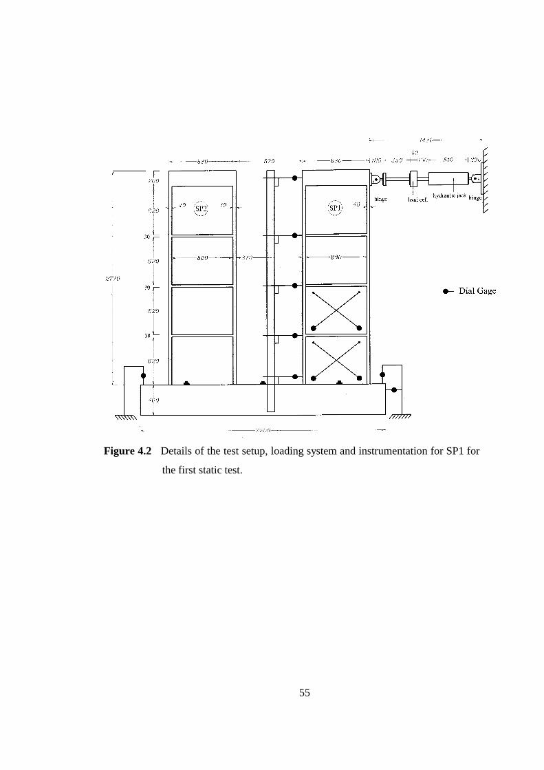
55
Figure 4.2 Details of the test setup, loading system and instrumentation for SP1 for
the first static test.
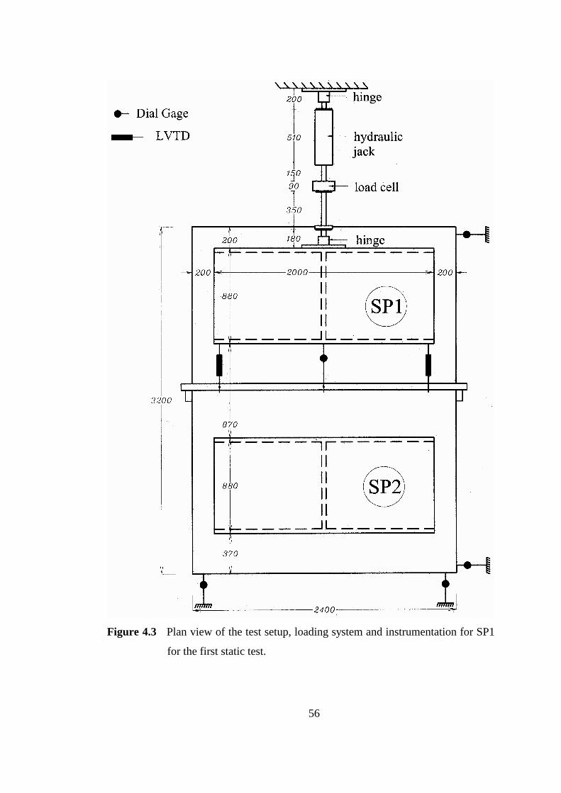
56
Figure 4.3 Plan view of the test setup, loading system and instrumentation for SP1
for the first static test.
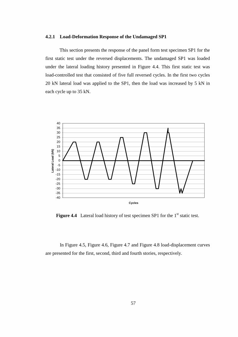
57
4.2.1 Load-Deformation Response of the Undamaged SP1
This section presents the response of the panel form test specimen SP1 for the
first static test under the reversed displacements. The undamaged SP1 was loaded
under the lateral loading history presented in Figure 4.4. This first static test was
load-controlled test that consisted of five full reversed cycles. In the first two cycles
20 kN lateral load was applied to the SP1, then the load was increased by 5 kN in
each cycle up to 35 kN.
-40-35-30-25-20-15-10-505
10152025303540
Cycles
Late
ral L
oad
(kN
)
Figure 4.4 Lateral load history of test specimen SP1 for the 1st static test.
In Figure 4.5, Figure 4.6, Figure 4.7 and Figure 4.8 load-displacement curves
are presented for the first, second, third and fourth stories, respectively.
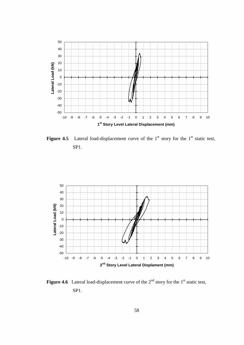
58
-50
-40
-30
-20
-10
0
10
20
30
40
50
-10 -9 -8 -7 -6 -5 -4 -3 -2 -1 0 1 2 3 4 5 6 7 8 9 10
1st Story Level Lateral Displacement (mm)
Late
ral L
oad
(kN
)
Figure 4.5 Lateral load-displacement curve of the 1st story for the 1st static test,
SP1.
-50
-40
-30
-20
-10
0
10
20
30
40
50
-10 -9 -8 -7 -6 -5 -4 -3 -2 -1 0 1 2 3 4 5 6 7 8 9 10
2nd Story Level Lateral Displament (mm)
Late
ral L
oad
(kN
)
Figure 4.6 Lateral load-displacement curve of the 2nd story for the 1st static test,
SP1.
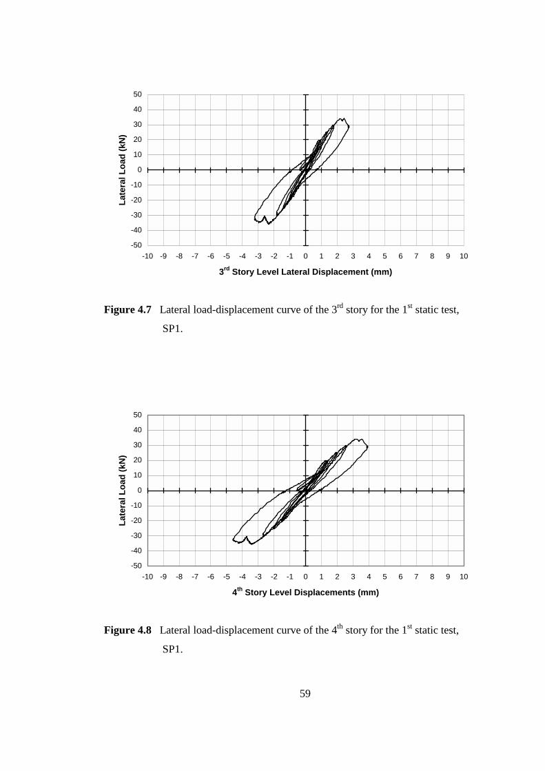
59
-50
-40
-30
-20
-10
0
10
20
30
40
50
-10 -9 -8 -7 -6 -5 -4 -3 -2 -1 0 1 2 3 4 5 6 7 8 9 10
3rd Story Level Lateral Displacement (mm)
Late
ral L
oad
(kN
)
Figure 4.7 Lateral load-displacement curve of the 3rd story for the 1st static test,
SP1.
-50
-40
-30
-20
-10
0
10
20
30
40
50
-10 -9 -8 -7 -6 -5 -4 -3 -2 -1 0 1 2 3 4 5 6 7 8 9 10
4th Story Level Displacements (mm)
Late
ral L
oad
(kN
)
Figure 4.8 Lateral load-displacement curve of the 4th story for the 1st static test,
SP1.

60
For the 1st static test of SP1, the top deflections are summarized in Table 4.1.
Table 4.1 Summary of the top deflection of the 1st static test of SP1.
Half cycle No Maximum top displacement (mm) Lateral load (kN)
1
-1
2
-2
3
-3
4
-4
5
-5
1.27
-1.46
1.40
-1.52
1.96
-2.00
2.53
-2.66
3.89
-4.60
20
-20
20
-20
25
-25
30
-30
35
-35
The maximum lateral load applied to SP1 for the 1st static test was 35 kN. At
this load level, the maximum top displacement of the SP1 was 4.6 mm.
The drift ratio of each story is calculated and plotted against the applied
lateral load. The displacements in these curves are relative and normalized with
respect to the story height. Variations of the 1st, 2nd, 3rd, and 4th story drift ratios for
the first static test of SP1 are presented in Figure 4.9, Figure 4.10, Figure 4.11 and
Figure 4.12, respectively.
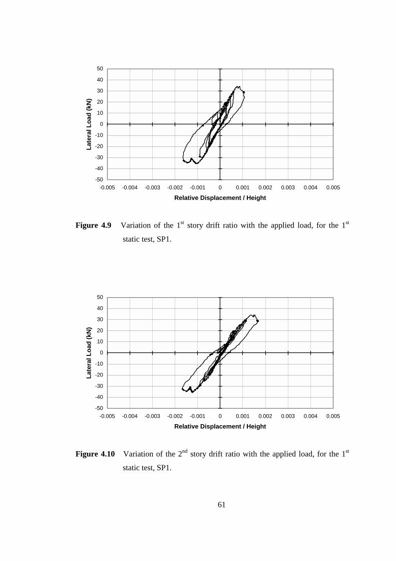
61
-50
-40
-30
-20
-10
0
10
20
30
40
50
-0.005 -0.004 -0.003 -0.002 -0.001 0 0.001 0.002 0.003 0.004 0.005
Relative Displacement / Height
Late
ral L
oad
(kN
)
Figure 4.9 Variation of the 1st story drift ratio with the applied load, for the 1st
static test, SP1.
-50
-40
-30
-20
-10
0
10
20
30
40
50
-0.005 -0.004 -0.003 -0.002 -0.001 0 0.001 0.002 0.003 0.004 0.005
Relative Displacement / Height
Late
ral L
oad
(kN
)
Figure 4.10 Variation of the 2nd story drift ratio with the applied load, for the 1st
static test, SP1.
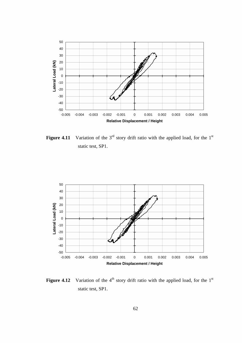
62
-50
-40
-30
-20
-10
0
10
20
30
40
50
-0.005 -0.004 -0.003 -0.002 -0.001 0 0.001 0.002 0.003 0.004 0.005
Relative Displacement / Height
Late
ral L
oad
(kN
)
Figure 4.11 Variation of the 3rd story drift ratio with the applied load, for the 1st
static test, SP1.
-50
-40
-30
-20
-10
0
10
20
30
40
50
-0.005 -0.004 -0.003 -0.002 -0.001 0 0.001 0.002 0.003 0.004 0.005
Relative Displacement / Height
Late
ral L
oad
(kN
)
Figure 4.12 Variation of the 4th story drift ratio with the applied load, for the 1st
static test, SP1.
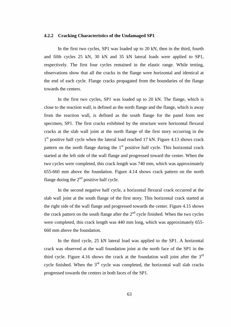
63
4.2.2 Cracking Characteristics of the Undamaged SP1
In the first two cycles, SP1 was loaded up to 20 kN, then in the third, fourth
and fifth cycles 25 kN, 30 kN and 35 kN lateral loads were applied to SP1,
respectively. The first four cycles remained in the elastic range. While testing,
observations show that all the cracks in the flange were horizontal and identical at
the end of each cycle. Flange cracks propagated from the boundaries of the flange
towards the centers.
In the first two cycles, SP1 was loaded up to 20 kN. The flange, which is
close to the reaction wall, is defined as the north flange and the flange, which is away
from the reaction wall, is defined as the south flange for the panel form test
specimen, SP1. The first cracks exhibited by the structure were horizontal flexural
cracks at the slab wall joint at the north flange of the first story occurring in the
1st positive half cycle when the lateral load reached 17 kN. Figure 4.13 shows crack
pattern on the north flange during the 1st positive half cycle. This horizontal crack
started at the left side of the wall flange and progressed toward the center. When the
two cycles were completed, this crack length was 740 mm, which was approximately
655-660 mm above the foundation. Figure 4.14 shows crack pattern on the north
flange during the 2nd positive half cycle.
In the second negative half cycle, a horizontal flexural crack occurred at the
slab wall joint at the south flange of the first story. This horizontal crack started at
the right side of the wall flange and progressed towards the center. Figure 4.15 shows
the crack pattern on the south flange after the 2nd cycle finished. When the two cycles
were completed, this crack length was 440 mm long, which was approximately 655-
660 mm above the foundation.
In the third cycle, 25 kN lateral load was applied to the SP1. A horizontal
crack was observed at the wall foundation joint at the north face of the SP1 in the
third cycle. Figure 4.16 shows the crack at the foundation wall joint after the 3rd
cycle finished. When the 3rd cycle was completed, the horizontal wall slab cracks
progressed towards the centers in both faces of the SP1.
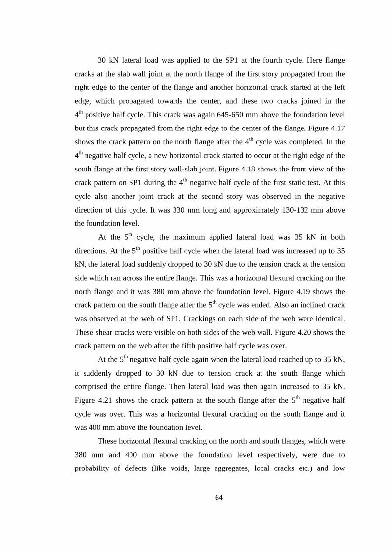
64
30 kN lateral load was applied to the SP1 at the fourth cycle. Here flange
cracks at the slab wall joint at the north flange of the first story propagated from the
right edge to the center of the flange and another horizontal crack started at the left
edge, which propagated towards the center, and these two cracks joined in the
4th positive half cycle. This crack was again 645-650 mm above the foundation level
but this crack propagated from the right edge to the center of the flange. Figure 4.17
shows the crack pattern on the north flange after the 4th cycle was completed. In the
4th negative half cycle, a new horizontal crack started to occur at the right edge of the
south flange at the first story wall-slab joint. Figure 4.18 shows the front view of the
crack pattern on SP1 during the 4th negative half cycle of the first static test. At this
cycle also another joint crack at the second story was observed in the negative
direction of this cycle. It was 330 mm long and approximately 130-132 mm above
the foundation level.
At the 5th cycle, the maximum applied lateral load was 35 kN in both
directions. At the 5th positive half cycle when the lateral load was increased up to 35
kN, the lateral load suddenly dropped to 30 kN due to the tension crack at the tension
side which ran across the entire flange. This was a horizontal flexural cracking on the
north flange and it was 380 mm above the foundation level. Figure 4.19 shows the
crack pattern on the south flange after the 5th cycle was ended. Also an inclined crack
was observed at the web of SP1. Crackings on each side of the web were identical.
These shear cracks were visible on both sides of the web wall. Figure 4.20 shows the
crack pattern on the web after the fifth positive half cycle was over.
At the 5th negative half cycle again when the lateral load reached up to 35 kN,
it suddenly dropped to 30 kN due to tension crack at the south flange which
comprised the entire flange. Then lateral load was then again increased to 35 kN.
Figure 4.21 shows the crack pattern at the south flange after the 5th negative half
cycle was over. This was a horizontal flexural cracking on the south flange and it
was 400 mm above the foundation level.
These horizontal flexural cracking on the north and south flanges, which were
380 mm and 400 mm above the foundation level respectively, were due to
probability of defects (like voids, large aggregates, local cracks etc.) and low
65
reinforcement ratio. Placing of the concrete of the panel form test specimens was
achieved in stages, therefore, while placing and compaction of the concrete, weak
construction surfaces occurred. While loading the test specimens, tension cracks
occurred at these weak surfaces such as foundation wall joints and first story slab
wall joints, which were 380-400 mm above the foundation level.
Figure 4.13 Crack pattern on the north flange during the 1st positive half cycle, 1st
static test, SP1.

66
Figure 4.14 Crack pattern on the north flange during the 2nd positive half cycle, 1st
static test, SP1.
Figure 4.15 Crack pattern on the south flange after the 2nd cycle finished, 1st static
test, SP1.

67
Figure 4.16 Crack at the foundation wall joint after the 3rd cycle finished, 1st static
test, SP1.
Figure 4.17 Crack pattern on the north flange after the 4th cycle finished, 1st static
test, SP1.
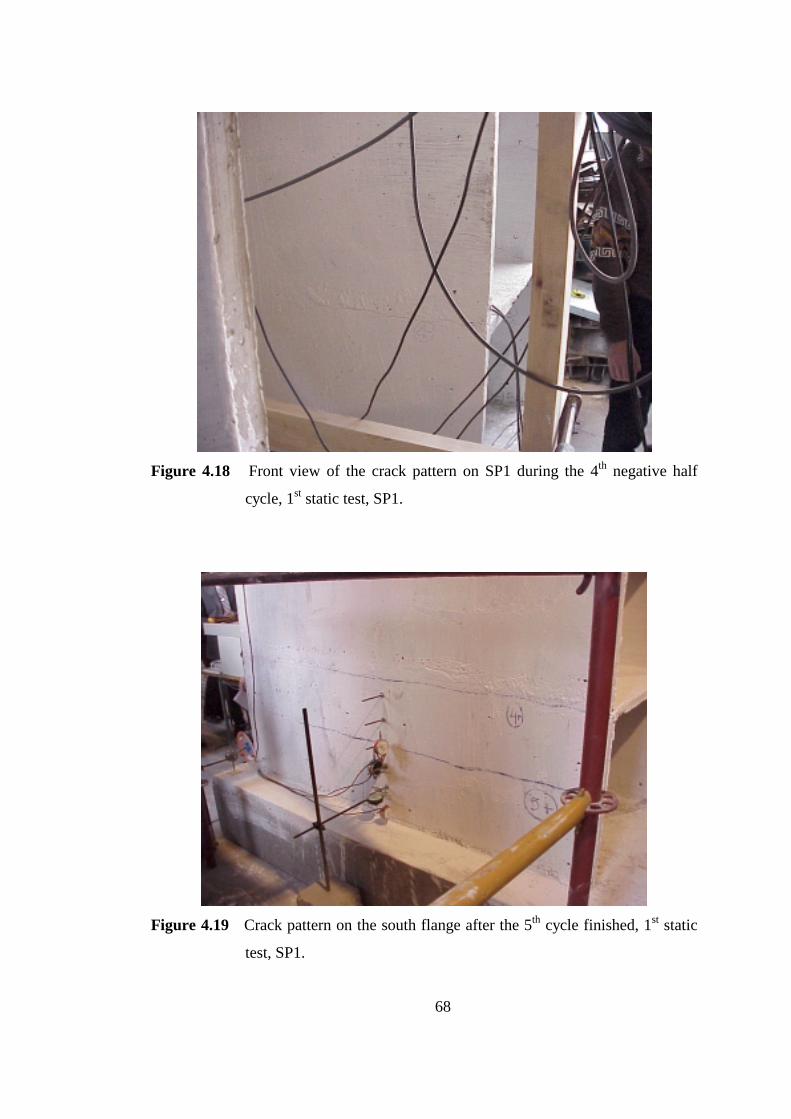
68
Figure 4.18 Front view of the crack pattern on SP1 during the 4th negative half
cycle, 1st static test, SP1.
Figure 4.19 Crack pattern on the south flange after the 5th cycle finished, 1st static
test, SP1.

69
Figure 4.20 Crack pattern on the web after the 5th positive half cycle finished, 1st
static test, SP1.
Figure 4.21 Crack pattern at the south flange after the 5th negative half cycle
finished, 1st static test, SP1.
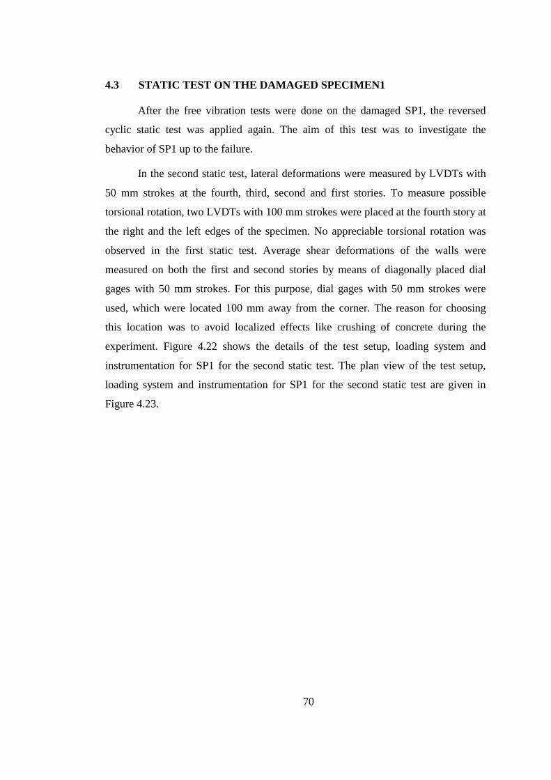
70
4.3 STATIC TEST ON THE DAMAGED SPECIMEN1
After the free vibration tests were done on the damaged SP1, the reversed
cyclic static test was applied again. The aim of this test was to investigate the
behavior of SP1 up to the failure.
In the second static test, lateral deformations were measured by LVDTs with
50 mm strokes at the fourth, third, second and first stories. To measure possible
torsional rotation, two LVDTs with 100 mm strokes were placed at the fourth story at
the right and the left edges of the specimen. No appreciable torsional rotation was
observed in the first static test. Average shear deformations of the walls were
measured on both the first and second stories by means of diagonally placed dial
gages with 50 mm strokes. For this purpose, dial gages with 50 mm strokes were
used, which were located 100 mm away from the corner. The reason for choosing
this location was to avoid localized effects like crushing of concrete during the
experiment. Figure 4.22 shows the details of the test setup, loading system and
instrumentation for SP1 for the second static test. The plan view of the test setup,
loading system and instrumentation for SP1 for the second static test are given in
Figure 4.23.

71
Figure 4.22 Details of the test setup, loading system and instrumentation for SP1
for the second static test.

72
Figure 4.23 Plan view of the test setup, loading system and instrumentation for SP1
for the second static test.
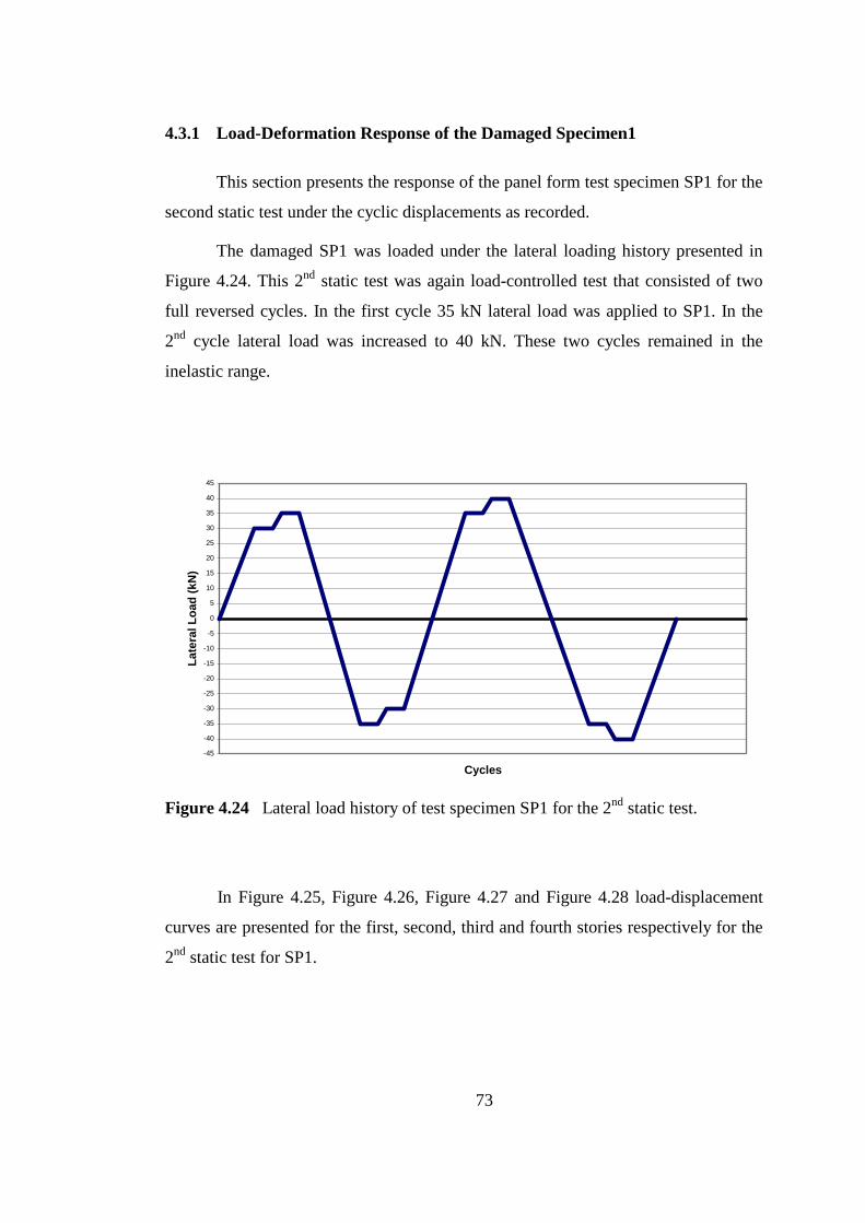
73
4.3.1 Load-Deformation Response of the Damaged Specimen1
This section presents the response of the panel form test specimen SP1 for the
second static test under the cyclic displacements as recorded.
The damaged SP1 was loaded under the lateral loading history presented in
Figure 4.24. This 2nd static test was again load-controlled test that consisted of two
full reversed cycles. In the first cycle 35 kN lateral load was applied to SP1. In the
2nd cycle lateral load was increased to 40 kN. These two cycles remained in the
inelastic range.
-45
-40
-35
-30
-25
-20
-15
-10
-5
0
5
10
15
20
25
30
35
40
45
Cycles
Late
ral L
oad
(kN
)
Figure 4.24 Lateral load history of test specimen SP1 for the 2nd static test.
In Figure 4.25, Figure 4.26, Figure 4.27 and Figure 4.28 load-displacement
curves are presented for the first, second, third and fourth stories respectively for the
2nd static test for SP1.
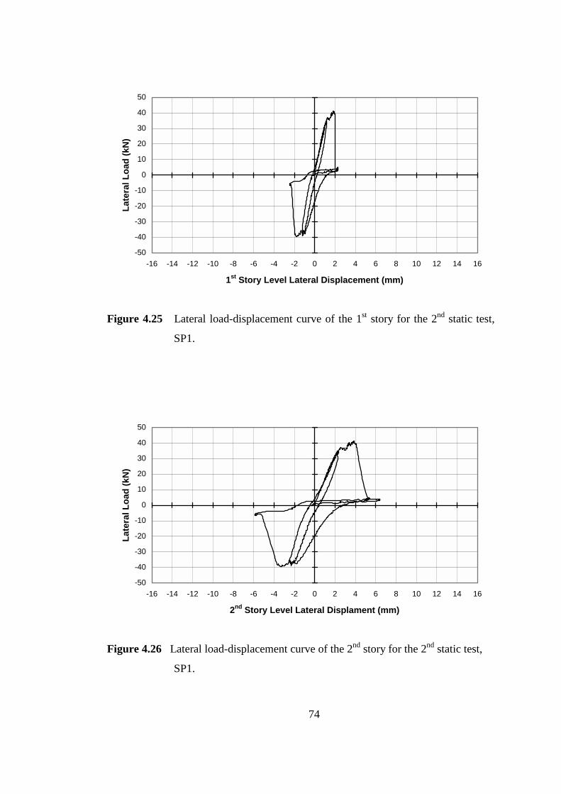
74
-50
-40
-30
-20
-10
0
10
20
30
40
50
-16 -14 -12 -10 -8 -6 -4 -2 0 2 4 6 8 10 12 14 16
1st Story Level Lateral Displacement (mm)
Late
ral L
oad
(kN
)
Figure 4.25 Lateral load-displacement curve of the 1st story for the 2nd static test,
SP1.
-50
-40
-30
-20
-10
0
10
20
30
40
50
-16 -14 -12 -10 -8 -6 -4 -2 0 2 4 6 8 10 12 14 16
2nd Story Level Lateral Displament (mm)
Late
ral L
oad
(kN
)
Figure 4.26 Lateral load-displacement curve of the 2nd story for the 2nd static test,
SP1.
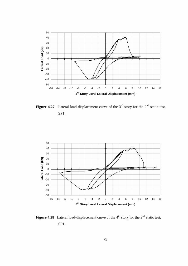
75
-50
-40
-30
-20
-10
0
10
20
30
40
50
-16 -14 -12 -10 -8 -6 -4 -2 0 2 4 6 8 10 12 14 16
3rd Story Level Lateral Displacement (mm)
Late
ral L
oad
(kN
)
Figure 4.27 Lateral load-displacement curve of the 3rd story for the 2nd static test,
SP1.
-50
-40
-30
-20
-10
0
10
20
30
40
50
-16 -14 -12 -10 -8 -6 -4 -2 0 2 4 6 8 10 12 14 16
4th Story Level Lateral Displacement (mm)
Late
ral L
oad
(kN
)
Figure 4.28 Lateral load-displacement curve of the 4th story for the 2nd static test,
SP1.
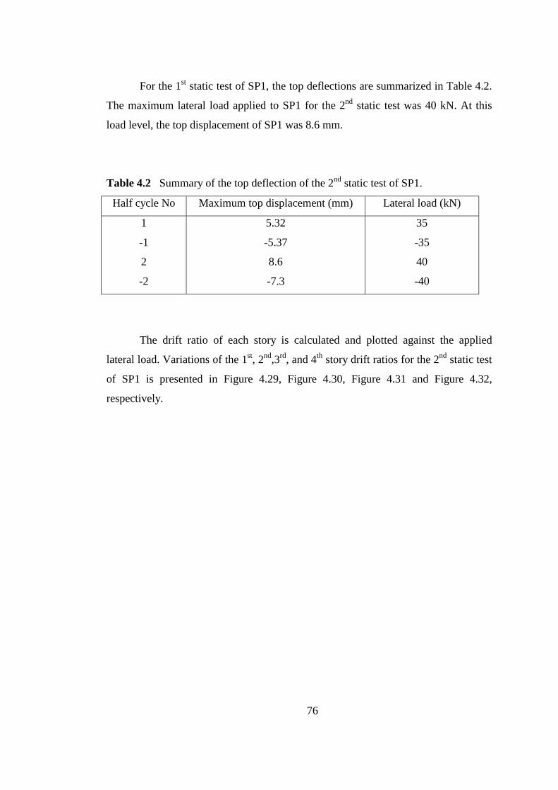
76
For the 1st static test of SP1, the top deflections are summarized in Table 4.2.
The maximum lateral load applied to SP1 for the 2nd static test was 40 kN. At this
load level, the top displacement of SP1 was 8.6 mm.
Table 4.2 Summary of the top deflection of the 2nd static test of SP1.
Half cycle No Maximum top displacement (mm) Lateral load (kN)
1
-1
2
-2
5.32
-5.37
8.6
-7.3
35
-35
40
-40
The drift ratio of each story is calculated and plotted against the applied
lateral load. Variations of the 1st, 2nd,3rd, and 4th story drift ratios for the 2nd static test
of SP1 is presented in Figure 4.29, Figure 4.30, Figure 4.31 and Figure 4.32,
respectively.

77
-50
-40
-30
-20
-10
0
10
20
30
40
50
-0.008 -0.006 -0.004 -0.002 0 0.002 0.004 0.006 0.008
Relative Displacement / Height
Late
ral L
oad
(kN
)
Figure 4.29 Variation of the 1st story drift ratio with the applied load, for the 2nd
static test, SP1.
-50
-40
-30
-20
-10
0
10
20
30
40
50
-0.008 -0.006 -0.004 -0.002 0 0.002 0.004 0.006 0.008
Relative Displacement / Height
Late
ral L
oad
(kN
)
Figure 4.30 Variation of the 2nd story drift ratio with the applied load, for the 2nd
static test, SP1.
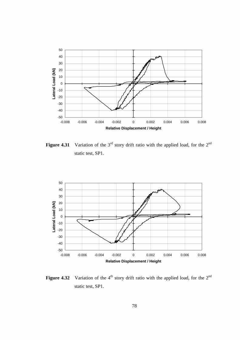
78
-50
-40
-30
-20
-10
0
10
20
30
40
50
-0.008 -0.006 -0.004 -0.002 0 0.002 0.004 0.006 0.008
Relative Displacement / Height
Late
ral L
oad
(kN
)
Figure 4.31 Variation of the 3rd story drift ratio with the applied load, for the 2nd
static test, SP1.
-50
-40
-30
-20
-10
0
10
20
30
40
50
-0.008 -0.006 -0.004 -0.002 0 0.002 0.004 0.006 0.008
Relative Displacement / Height
Late
ral L
oad
(kN
)
Figure 4.32 Variation of the 4th story drift ratio with the applied load, for the 2nd
static test, SP1.
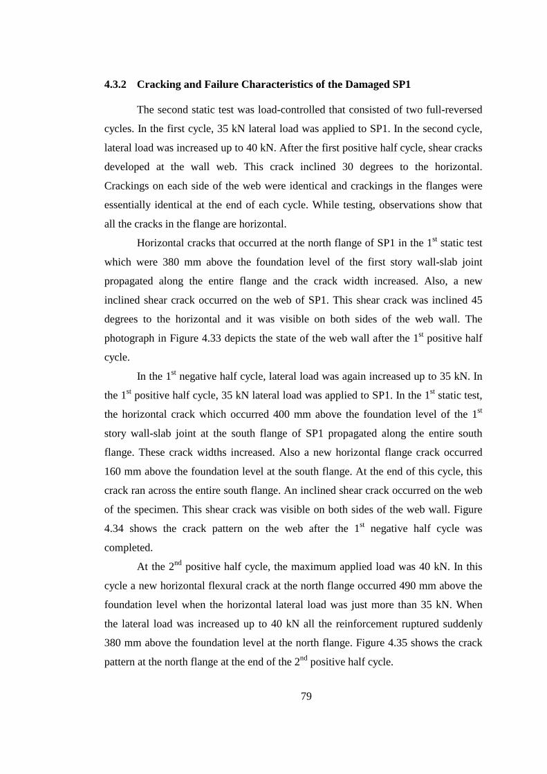
79
4.3.2 Cracking and Failure Characteristics of the Damaged SP1
The second static test was load-controlled that consisted of two full-reversed
cycles. In the first cycle, 35 kN lateral load was applied to SP1. In the second cycle,
lateral load was increased up to 40 kN. After the first positive half cycle, shear cracks
developed at the wall web. This crack inclined 30 degrees to the horizontal.
Crackings on each side of the web were identical and crackings in the flanges were
essentially identical at the end of each cycle. While testing, observations show that
all the cracks in the flange are horizontal.
Horizontal cracks that occurred at the north flange of SP1 in the 1st static test
which were 380 mm above the foundation level of the first story wall-slab joint
propagated along the entire flange and the crack width increased. Also, a new
inclined shear crack occurred on the web of SP1. This shear crack was inclined 45
degrees to the horizontal and it was visible on both sides of the web wall. The
photograph in Figure 4.33 depicts the state of the web wall after the 1st positive half
cycle.
In the 1st negative half cycle, lateral load was again increased up to 35 kN. In
the 1st positive half cycle, 35 kN lateral load was applied to SP1. In the 1st static test,
the horizontal crack which occurred 400 mm above the foundation level of the 1st
story wall-slab joint at the south flange of SP1 propagated along the entire south
flange. These crack widths increased. Also a new horizontal flange crack occurred
160 mm above the foundation level at the south flange. At the end of this cycle, this
crack ran across the entire south flange. An inclined shear crack occurred on the web
of the specimen. This shear crack was visible on both sides of the web wall. Figure
4.34 shows the crack pattern on the web after the 1st negative half cycle was
completed.
At the 2nd positive half cycle, the maximum applied load was 40 kN. In this
cycle a new horizontal flexural crack at the north flange occurred 490 mm above the
foundation level when the horizontal lateral load was just more than 35 kN. When
the lateral load was increased up to 40 kN all the reinforcement ruptured suddenly
380 mm above the foundation level at the north flange. Figure 4.35 shows the crack
pattern at the north flange at the end of the 2nd positive half cycle.

80
At the 2nd negative half cycle, lateral load increased up to 40 kN. When the
horizontal lateral load was just more than 35 kN, a horizontal flexural crack
420 mm above the foundation level occurred at the south flange of SP1. This
horizontal flange crack occurred at the right edge of the flange and propagated
towards the center. The crack length was 480 mm. When the lateral load reached 40
kN, all the reinforcement in the south flange ruptured suddenly 380 mm above the
foundation level. Figure 4.36 shows the crack pattern at the south flange when the 2nd
negative half cycle ended. Figure 4.37 shows the crack pattern on the web of SP1
after the 2nd negative half cycle. At this stage, the second static test for the damaged
SP1 was over.
The failure of SP1 was due to the rupturing of the longitudinal reinforcement
bars in the flange. The failure was very unpredictable and brittle. In the 2nd positive
half cycle when the lateral load reached up to 40 kN, all the longitudinal
reinforcement in the north flange ruptured 380 mm above the foundation level.
Figure 4.39 shows the photograph of the reinforcement rupturing at the north flange
of SP1 after the 2nd static test. In the 2nd negative half cycle, again all the longitudinal
reinforcement in the south flange ruptured 380 mm above the foundation level at the
lateral load level of 40 kN. Figure 4.40 shows the photograph of the reinforcement
rupturing at the south flange of SP1 after the 2nd static test. All the mesh
reinforcement in the flange ruptured below the welded points of the longitudinal and
the horizontal reinforcement. Crushing of the concrete was not observed in the static
tests of SP1.
The moment at the failure surface, which was approximately 400 mm above
the foundation level, was 85% of the maximum moment. Deformation was
accumulated on the failure surface. If the reinforcement ratio had been higher, it
might have prevented the failure at the cracking location. More horizontal cracks
might have occurred near or at the maximum moment regions. Due to low
longitudinal reinforcement ratio, as soon as the concrete cracked at the weak surface,
longitudinal reinforcements yielded and ruptured at these crack surfaces. If the
longitudinal reinforcement ratio had been higher, longitudinal reinforcement would
not have yielded and ruptured as soon as concrete cracked 380-400 mm above the

81
foundation and new horizontal cracks would have occurred near or at the maximum
moment regions. Plastic hinge and crushing of concrete would have occurred
according to the amount of longitudinal reinforcement ratio. The failure of SP1
would have been at the maximum moment region.
Figure 4.33 Crack pattern on the web after the 1st positive half cycle finished, 2nd
static test, SP1.

82
Figure 4.34 Crack pattern on the web after the 1st negative half cycle finished, 2nd
static test, SP1.
Figure 4.35 Crack pattern at the north flange after the 2nd positive half cycle
finished, 2nd static test, SP1.

83
Figure 4.36 Crack pattern at the south flange after the 2nd negative half cycle
finished, 2nd static test SP1.
Figure 4.37 Crack pattern on the web of SP1 after the 2nd negative half cycle, 2nd
static test.
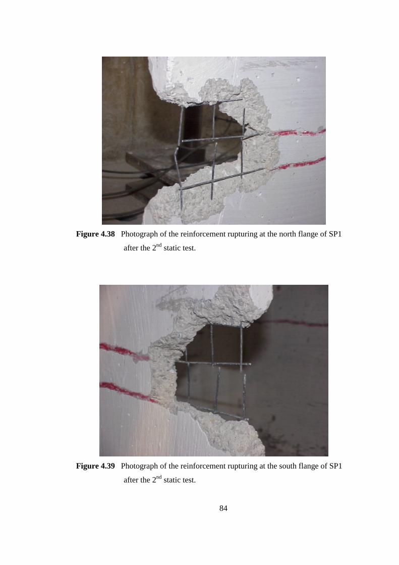
84
Figure 4.38 Photograph of the reinforcement rupturing at the north flange of SP1
after the 2nd static test.
Figure 4.39 Photograph of the reinforcement rupturing at the south flange of SP1
after the 2nd static test.
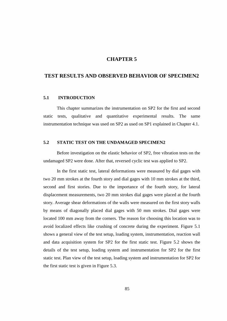
85
CHAPTER 5 TEST RESULTS AND OBSERVED BEHAVIOR OF SPECIMEN2
5.1 INTRODUCTION
This chapter summarizes the instrumentation on SP2 for the first and second
static tests, qualitative and quantitative experimental results. The same
instrumentation technique was used on SP2 as used on SP1 explained in Chapter 4.1.
5.2 STATIC TEST ON THE UNDAMAGED SPECIMEN2
Before investigation on the elastic behavior of SP2, free vibration tests on the
undamaged SP2 were done. After that, reversed cyclic test was applied to SP2.
In the first static test, lateral deformations were measured by dial gages with
two 20 mm strokes at the fourth story and dial gages with 10 mm strokes at the third,
second and first stories. Due to the importance of the fourth story, for lateral
displacement measurements, two 20 mm strokes dial gages were placed at the fourth
story. Average shear deformations of the walls were measured on the first story walls
by means of diagonally placed dial gages with 50 mm strokes. Dial gages were
located 100 mm away from the corners. The reason for choosing this location was to
avoid localized effects like crushing of concrete during the experiment. Figure 5.1
shows a general view of the test setup, loading system, instrumentation, reaction wall
and data acquisition system for SP2 for the first static test. Figure 5.2 shows the
details of the test setup, loading system and instrumentation for SP2 for the first
static test. Plan view of the test setup, loading system and instrumentation for SP2 for
the first static test is given in Figure 5.3.

86
Figure 5.1 A general view of the test setup, loading system, instrumentation,
reaction wall and data acquisition system for SP2 for the 1st static test.
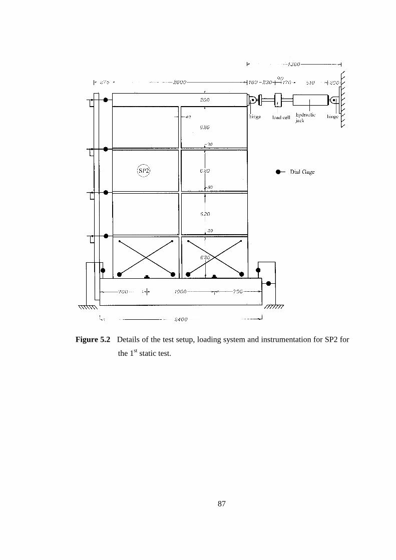
87
Figure 5.2 Details of the test setup, loading system and instrumentation for SP2 for
the 1st static test.
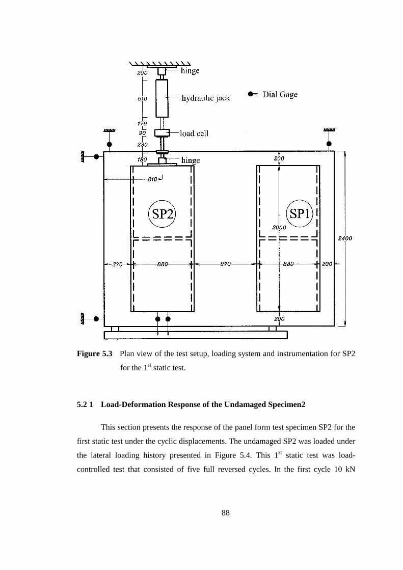
88
Figure 5.3 Plan view of the test setup, loading system and instrumentation for SP2
for the 1st static test.
5.2 1 Load-Deformation Response of the Undamaged Specimen2
This section presents the response of the panel form test specimen SP2 for the
first static test under the cyclic displacements. The undamaged SP2 was loaded under
the lateral loading history presented in Figure 5.4. This 1st static test was load-
controlled test that consisted of five full reversed cycles. In the first cycle 10 kN
89
lateral load was applied to SP2, then the load was increased by 5 kN in each cycle up
to 30 kN.
The maximum lateral load applied to SP2 for the first static test was 33 kN.
At this load level, the top displacement of SP2 was 1.142 mm. In Figure 5.5, Figure
5.6, Figure 5.7 and Figure 5.8 load-displacement curves are presented for the 1st, 2nd,
3rd and 4th stories, respectively.
-40
-35
-30
-25
-20
-15
-10
-5
0
5
10
15
20
25
30
35
Cycles
Late
ral L
oad
(kN
)
Figure 5.4 Lateral load history of the test specimen SP2 for the 1st static test.
90
-40
-30
-20
-10
0
10
20
30
40
-3.0 -2.5 -2.0 -1.5 -1.0 -0.5 0.0 0.5 1.0 1.5 2.0 2.5 3.0
1st Story Level Lateral Displacement (mm)
Late
ral L
oad
(kN
)
Figure 5.5 Lateral load-displacement curve of the 1st story for the 1st static test,
SP2.
-40
-30
-20
-10
0
10
20
30
40
-3.0 -2.5 -2.0 -1.5 -1.0 -0.5 0.0 0.5 1.0 1.5 2.0 2.5 3.0
2nd Story Level Lateral Displacement (mm)
Late
ral L
oad
(kN
)
Figure 5.6 Lateral load-displacement curve of the 2nd story for the 1st static test,
SP2.
91
-40
-30
-20
-10
0
10
20
30
40
-3.0 -2.5 -2.0 -1.5 -1.0 -0.5 0.0 0.5 1.0 1.5 2.0 2.5 3.0
3rd Story Level Lateral Displacement (mm)
Late
ral L
oad
(kN
)
Figure 5.7 Lateral load-displacement curve of the 3rd story for the 1st static test,
SP2.
-40
-30
-20
-10
0
10
20
30
40
-3.0 -2.5 -2.0 -1.5 -1.0 -0.5 0.0 0.5 1.0 1.5 2.0 2.5 3.04th Story Level Lateral Displacement (mm)
Late
ral L
oad
(kN
)
Figure 5.8 Lateral load-displacement curve of the 4th story for the 1st static test,
SP2.

92
For the 1st static test of SP2 the top deflections are summarized in Table 5.1.
The maximum lateral load applied to SP2 for the 2nd static test was 30 kN. At this
load level, the top displacement of SP2 was 1.016 mm.
Table 5.1 Summary of the top deflection of the 1st static test of SP2.
Half cycle No Maximum top displacement (mm) Lateral load (kN)
1
-1
2
-2
3
-3
4
-4
5
-5
0.234
-0.322
0.352
-0.498
0.498
-0.664
0.654
-0.830
0.810
-1.016
10.0
-10.0
15.0
-15.0
20.0
-20.0
25.0
-25.0
30.0
-30.0
The drift ratio of each story is calculated and plotted against the applied
lateral load. Variations of the 1st, 2nd, 3rd, and 4th story drift ratios for the first static
test of SP2 are presented in Figure 5.9, Figure 5.10, Figure 5.11 and Figure 5.12,
respectively.
93
-40
-30
-20
-10
0
10
20
30
40
-0.003 -0.002 -0.001 0 0.001 0.002 0.003
Relative Displacement / Height
Late
ral L
oad
(kN
)
Figure 5.9 Variation of the 1st story drift ratio with the applied load, for the 1st
static test, SP2.
-40
-30
-20
-10
0
10
20
30
40
-0.003 -0.002 -0.001 0 0.001 0.002 0.003
Relative Displacement / Height
Late
ral L
oad
(kN
)
Figure 5.10 Variation of the 2nd story drift ratio with the applied load, for the 1st
static test, SP2.

94
-40
-30
-20
-10
0
10
20
30
40
-0.003 -0.002 -0.001 0 0.001 0.002 0.003
Relative Displacement / Height
Late
ral L
oad
(kN
)
Figure 5.11 Variation of the 3rd story drift ratio with the applied load, for the 1st
static test, SP2.
-40
-30
-20
-10
0
10
20
30
40
-0.003 -0.002 -0.001 0 0.001 0.002 0.003
Relative Displacement / Height
Late
ral L
oad
(kN
)
Figure 5.12 Variation of the 4th story drift ratio with the applied load, for the 1st
static test, SP2.
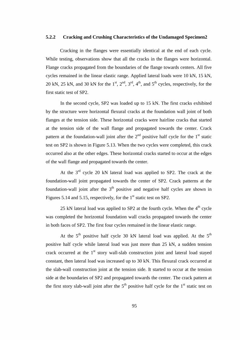
95
5.2.2 Cracking and Crushing Characteristics of the Undamaged Specimen2
Cracking in the flanges were essentially identical at the end of each cycle.
While testing, observations show that all the cracks in the flanges were horizontal.
Flange cracks propagated from the boundaries of the flange towards centers. All five
cycles remained in the linear elastic range. Applied lateral loads were 10 kN, 15 kN,
20 kN, 25 kN, and 30 kN for the 1st, 2nd, 3rd, 4th, and 5th cycles, respectively, for the
first static test of SP2.
In the second cycle, SP2 was loaded up to 15 kN. The first cracks exhibited
by the structure were horizontal flexural cracks at the foundation wall joint of both
flanges at the tension side. These horizontal cracks were hairline cracks that started
at the tension side of the wall flange and propagated towards the center. Crack
pattern at the foundation-wall joint after the 2nd positive half cycle for the 1st static
test on SP2 is shown in Figure 5.13. When the two cycles were completed, this crack
occurred also at the other edges. These horizontal cracks started to occur at the edges
of the wall flange and propagated towards the center.
At the 3rd cycle 20 kN lateral load was applied to SP2. The crack at the
foundation-wall joint propagated towards the center of SP2. Crack patterns at the
foundation-wall joint after the 3th positive and negative half cycles are shown in
Figures 5.14 and 5.15, respectively, for the 1st static test on SP2.
25 kN lateral load was applied to SP2 at the fourth cycle. When the 4th cycle
was completed the horizontal foundation wall cracks propagated towards the center
in both faces of SP2. The first four cycles remained in the linear elastic range.
At the 5th positive half cycle 30 kN lateral load was applied. At the 5th
positive half cycle while lateral load was just more than 25 kN, a sudden tension
crack occurred at the 1st story wall-slab construction joint and lateral load stayed
constant, then lateral load was increased up to 30 kN. This flexural crack occurred at
the slab-wall construction joint at the tension side. It started to occur at the tension
side at the boundaries of SP2 and propagated towards the center. The crack pattern at
the first story slab-wall joint after the 5th positive half cycle for the 1st static test on

96
SP2 is shown in Figure 5.16. At the negative 5th half cycle the maximum applied
lateral load was 32.65 kN. At the 5th negative half cycle when the lateral load was
just more than 25 kN again a tension crack occurred at the tension side at the1st story
wall-slab construction joint. When the lateral load was more than 30 kN the tension
crack propagated through neutral axis and when the lateral load reached 32.8 kN the
1st static test was ended.
Figure 5.13 Crack pattern at the foundation-wall joint after the 2nd positive half
cycle for the 1st static test on SP2.
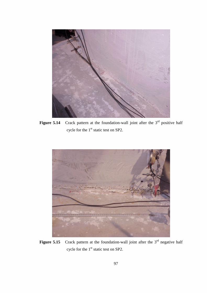
97
Figure 5.14 Crack pattern at the foundation-wall joint after the 3rd positive half
cycle for the 1st static test on SP2.
Figure 5.15 Crack pattern at the foundation-wall joint after the 3rd negative half
cycle for the 1st static test on SP2.

98
Figure 5.16 Crack pattern at the first story slab-wall joint after the 5th negative half
cycle for the 1st static test on SP2.
5.3 STATIC TEST ON THE DAMAGED SPECIMEN2
After the free vibration tests were done on the damaged SP2, the reversed
cyclic static test was applied again. The aim of this test was to investigate the
behavior of SP2 up to failure.
In the 2nd static test lateral deformations were measured by LVDTs with
50 mm strokes at the 4th, 3rd, 2nd and 1st stories. Average shear deformations of the
walls were measured on both the first and second stories by means of diagonally
placed dial gages with 50 mm strokes. For this purpose, dial gages with 50 mm
strokes were used. Dial gages were located 100 mm away from the corner. The
reason for choosing this location was to avoid localized effects like crushing of
concrete during the experiment. Figure 5.17 shows the details of the test setup,
loading system and instrumentation for SP2 for the 2nd static test. The plan view of

99
the test setup, loading system and instrumentation for SP2 for the 2nd static test are
given in Figure 5.18.
Figure 5.17 Details of the test setup, loading system and instrumentation for SP2
for the 2nd static test.

100
Figure 5.18 Plan view of the test setup, loading system and instrumentation for SP2
for the 2nd static test.
5.3.1 LOAD-DEFORMATION RESPONSE OF DAMAGED SPECIMEN2
This section presents the response of the panel form test specimen SP2 for the
2nd static test under the cyclic displacements.
The damaged SP2 was loaded under the lateral loading history presented in
Figure 5.19. This 2nd static test was again a load-controlled test that consisted of five
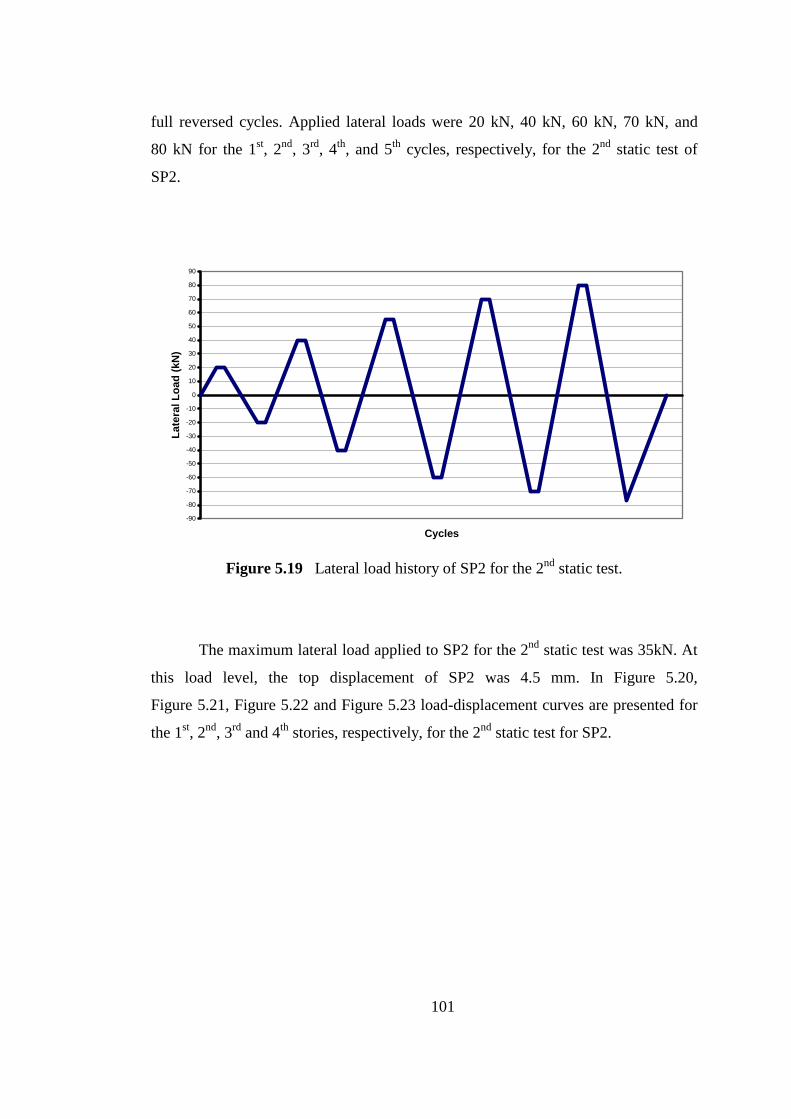
101
full reversed cycles. Applied lateral loads were 20 kN, 40 kN, 60 kN, 70 kN, and
80 kN for the 1st, 2nd, 3rd, 4th, and 5th cycles, respectively, for the 2nd static test of
SP2.
-90
-80
-70
-60
-50
-40
-30
-20
-10
0
10
20
30
40
50
60
70
80
90
Cycles
Late
ral L
oad
(kN
)
Figure 5.19 Lateral load history of SP2 for the 2nd static test.
The maximum lateral load applied to SP2 for the 2nd static test was 35kN. At
this load level, the top displacement of SP2 was 4.5 mm. In Figure 5.20,
Figure 5.21, Figure 5.22 and Figure 5.23 load-displacement curves are presented for
the 1st, 2nd, 3rd and 4th stories, respectively, for the 2nd static test for SP2.

102
-80
-60
-40
-20
0
20
40
60
80
-6 -5 -4 -3 -2 -1 0 1 2 3 4 5 6
1st Story Level Lateral Displacement (mm)
Late
ral L
oad
(kN
)
Figure 5.20 Lateral load-displacement curve of the 1st story for the 2nd static test,
SP2.
-80
-60
-40
-20
0
20
40
60
80
-6 -5 -4 -3 -2 -1 0 1 2 3 4 5 6
2nd Story Level Lateral Displacement (mm)
Late
ral L
oad
(kN
)
Figure 5.21 Lateral load-displacement curve of the 2nd story for the 2nd static test,
SP2.

103
-80
-60
-40
-20
0
20
40
60
80
-6 -5 -4 -3 -2 -1 0 1 2 3 4 5 6
3rd Story Level Lateral Displacement (mm)
Late
ral L
oad
(kN
)
Figure 5.22 Lateral load-displacement curve of the 3rd story for the 2nd static test,
SP2.
-80
-60
-40
-20
0
20
40
60
80
-6 -5 -4 -3 -2 -1 0 1 2 3 4 5 6
4th Story Level Lateral Displacement (mm)
Late
ral L
oad
(kN
)
Figure 5.23 Lateral load-displacement curve of the 4th story for the 2nd static test,
SP2.
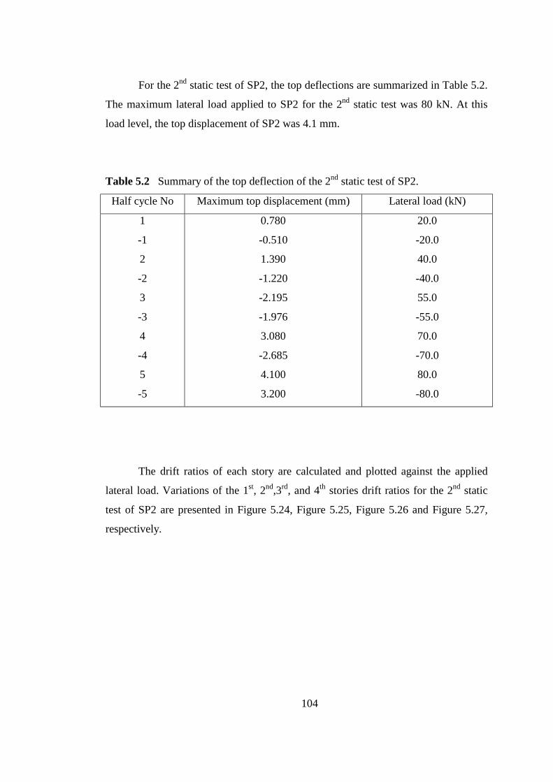
104
For the 2nd static test of SP2, the top deflections are summarized in Table 5.2.
The maximum lateral load applied to SP2 for the 2nd static test was 80 kN. At this
load level, the top displacement of SP2 was 4.1 mm.
Table 5.2 Summary of the top deflection of the 2nd static test of SP2.
Half cycle No Maximum top displacement (mm) Lateral load (kN)
1
-1
2
-2
3
-3
4
-4
5
-5
0.780
-0.510
1.390
-1.220
-2.195
-1.976
3.080
-2.685
4.100
3.200
20.0
-20.0
40.0
-40.0
55.0
-55.0
70.0
-70.0
80.0
-80.0
The drift ratios of each story are calculated and plotted against the applied
lateral load. Variations of the 1st, 2nd,3rd, and 4th stories drift ratios for the 2nd static
test of SP2 are presented in Figure 5.24, Figure 5.25, Figure 5.26 and Figure 5.27,
respectively.

105
-80
-60
-40
-20
0
20
40
60
80
-0.005 -0.004 -0.003 -0.002 -0.001 0 0.001 0.002 0.003 0.004 0.005
Relative Displacement / Height
Late
ral L
oad
(kN
)
Figure 5.24 Variation of the 1st story drift ratio with the applied load, for the 2nd
static test, SP2.
-80
-60
-40
-20
0
20
40
60
80
-0.005 -0.004 -0.003 -0.002 -0.001 0 0.001 0.002 0.003 0.004 0.005
Relative Displacement / Height
Late
ral L
oad
(kN
)
Figure 5.25 Variation of the 2nd story drift ratio with the applied load, for the 2nd
static test, SP2.
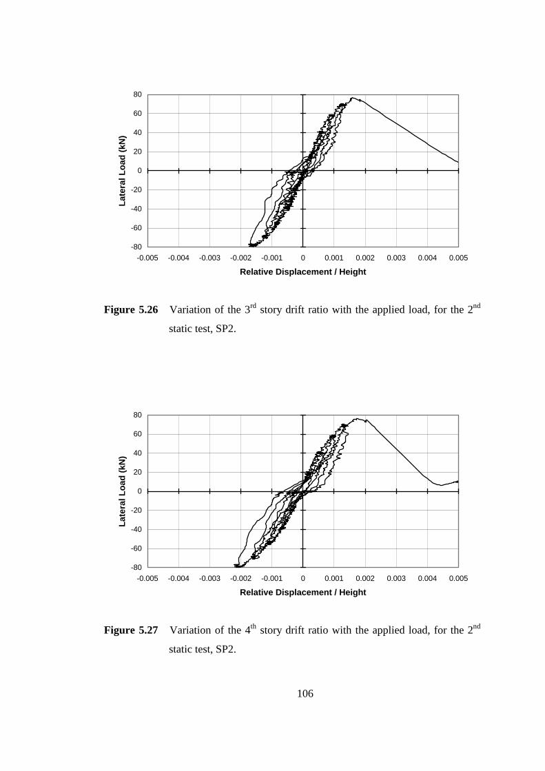
106
-80
-60
-40
-20
0
20
40
60
80
-0.005 -0.004 -0.003 -0.002 -0.001 0 0.001 0.002 0.003 0.004 0.005
Relative Displacement / Height
Late
ral L
oad
(kN
)
Figure 5.26 Variation of the 3rd story drift ratio with the applied load, for the 2nd
static test, SP2.
-80
-60
-40
-20
0
20
40
60
80
-0.005 -0.004 -0.003 -0.002 -0.001 0 0.001 0.002 0.003 0.004 0.005
Relative Displacement / Height
Late
ral L
oad
(kN
)
Figure 5.27 Variation of the 4th story drift ratio with the applied load, for the 2nd
static test, SP2.
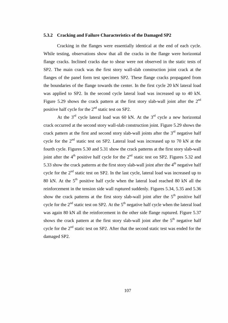
107
5.3.2 Cracking and Failure Characteristics of the Damaged SP2
Cracking in the flanges were essentially identical at the end of each cycle.
While testing, observations show that all the cracks in the flange were horizontal
flange cracks. Inclined cracks due to shear were not observed in the static tests of
SP2. The main crack was the first story wall-slab construction joint crack at the
flanges of the panel form test specimen SP2. These flange cracks propagated from
the boundaries of the flange towards the center. In the first cycle 20 kN lateral load
was applied to SP2. In the second cycle lateral load was increased up to 40 kN.
Figure 5.29 shows the crack pattern at the first story slab-wall joint after the 2nd
positive half cycle for the 2nd static test on SP2.
At the 3rd cycle lateral load was 60 kN. At the 3rd cycle a new horizontal
crack occurred at the second story wall-slab construction joint. Figure 5.29 shows the
crack pattern at the first and second story slab-wall joints after the 3rd negative half
cycle for the 2nd static test on SP2. Lateral load was increased up to 70 kN at the
fourth cycle. Figures 5.30 and 5.31 show the crack patterns at the first story slab-wall
joint after the 4th positive half cycle for the 2nd static test on SP2. Figures 5.32 and
5.33 show the crack patterns at the first story slab-wall joint after the 4th negative half
cycle for the 2nd static test on SP2. In the last cycle, lateral load was increased up to
80 kN. At the 5th positive half cycle when the lateral load reached 80 kN all the
reinforcement in the tension side wall ruptured suddenly. Figures 5.34, 5.35 and 5.36
show the crack patterns at the first story slab-wall joint after the 5th positive half
cycle for the 2nd static test on SP2. At the 5th negative half cycle when the lateral load
was again 80 kN all the reinforcement in the other side flange ruptured. Figure 5.37
shows the crack pattern at the first story slab-wall joint after the 5th negative half
cycle for the 2nd static test on SP2. After that the second static test was ended for the
damaged SP2.

108
Figure 5.28 Crack pattern at the first story slab-wall joint after the 2nd positive half
cycle for the 2nd static test on SP2.
Figure 5.29 Crack pattern at the first and second story slab-wall joint after the 3rd
negative half cycle for the 2nd static test on SP2.
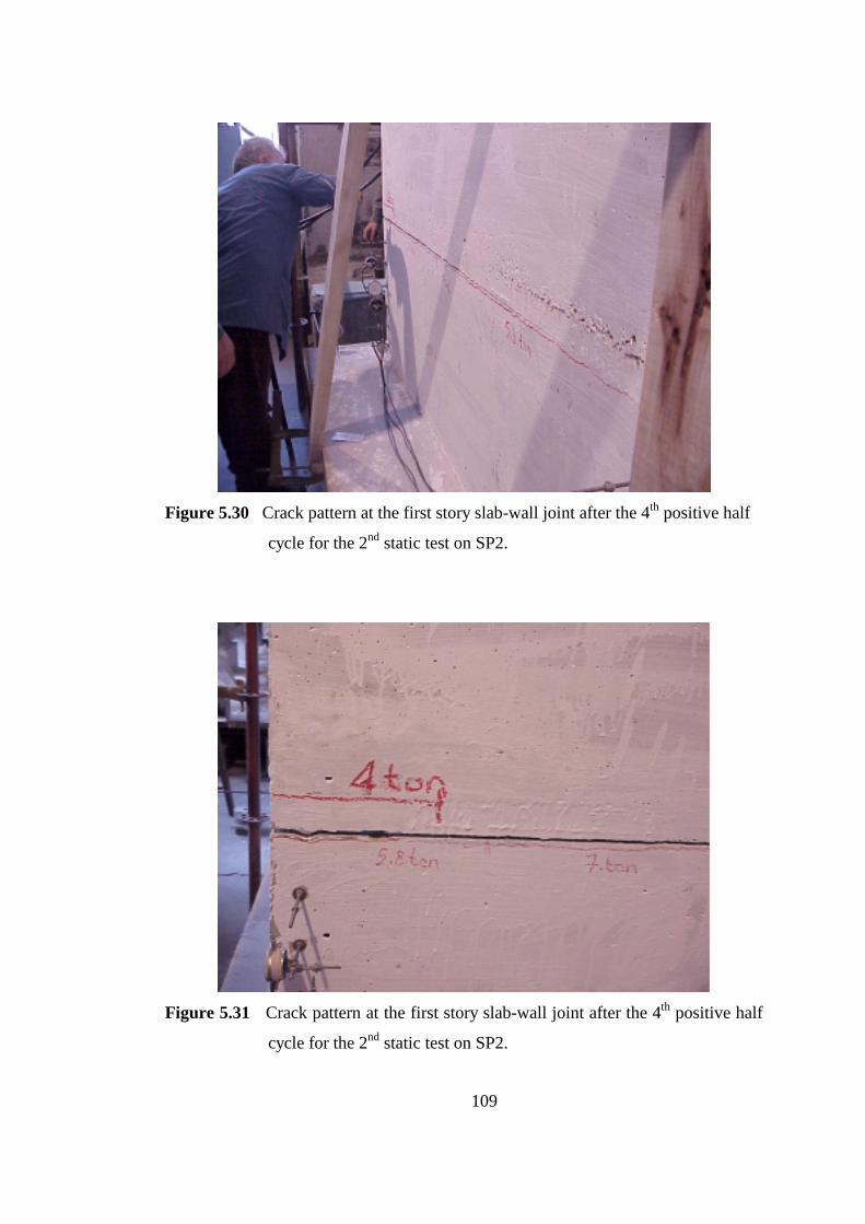
109
Figure 5.30 Crack pattern at the first story slab-wall joint after the 4th positive half
cycle for the 2nd static test on SP2.
Figure 5.31 Crack pattern at the first story slab-wall joint after the 4th positive half
cycle for the 2nd static test on SP2.
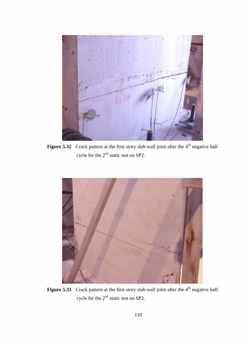
110
Figure 5.32 Crack pattern at the first story slab-wall joint after the 4th negative half
cycle for the 2nd static test on SP2.
Figure 5.33 Crack pattern at the first story slab-wall joint after the 4th negative half
cycle for the 2nd static test on SP2.

111
Figure 5.34 Crack pattern at the first story slab-wall joint after the 5th positive half
cycle for the 2nd static test on SP2.
Figure 5.35 Crack pattern at the first story slab-wall joint after the 5th positive half
cycle for the 2nd static test on SP2.
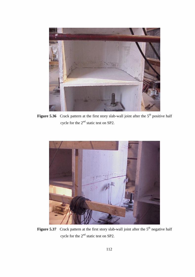
112
Figure 5.36 Crack pattern at the first story slab-wall joint after the 5th positive half
cycle for the 2nd static test on SP2.
Figure 5.37 Crack pattern at the first story slab-wall joint after the 5th negative half
cycle for the 2nd static test on SP2.

113
SP2 failed due to rupturing of the longitudinal mesh reinforcement of flanges
at the first story wall-slab construction joint. This failure occurred in a very sudden
and unpredictable manner. All the mesh reinforcement in the flange ruptured below
the welded point of the longitudinal and the horizontal reinforcement. Crushing of
the concrete was not observed in the static tests of SP2.
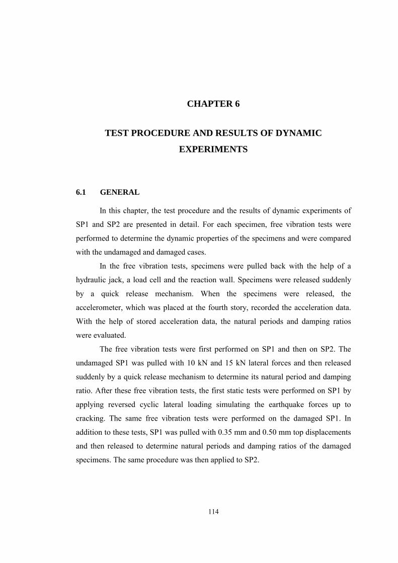
114
CHAPTER 6
TEST PROCEDURE AND RESULTS OF DYNAMIC
EXPERIMENTS
6.1 GENERAL
In this chapter, the test procedure and the results of dynamic experiments of
SP1 and SP2 are presented in detail. For each specimen, free vibration tests were
performed to determine the dynamic properties of the specimens and were compared
with the undamaged and damaged cases.
In the free vibration tests, specimens were pulled back with the help of a
hydraulic jack, a load cell and the reaction wall. Specimens were released suddenly
by a quick release mechanism. When the specimens were released, the
accelerometer, which was placed at the fourth story, recorded the acceleration data.
With the help of stored acceleration data, the natural periods and damping ratios
were evaluated.
The free vibration tests were first performed on SP1 and then on SP2. The
undamaged SP1 was pulled with 10 kN and 15 kN lateral forces and then released
suddenly by a quick release mechanism to determine its natural period and damping
ratio. After these free vibration tests, the first static tests were performed on SP1 by
applying reversed cyclic lateral loading simulating the earthquake forces up to
cracking. The same free vibration tests were performed on the damaged SP1. In
addition to these tests, SP1 was pulled with 0.35 mm and 0.50 mm top displacements
and then released to determine natural periods and damping ratios of the damaged
specimens. The same procedure was then applied to SP2.
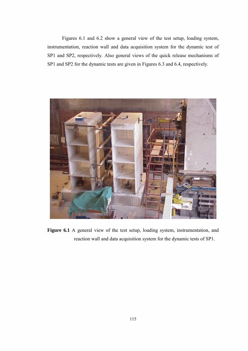
115
Figures 6.1 and 6.2 show a general view of the test setup, loading system,
instrumentation, reaction wall and data acquisition system for the dynamic test of
SP1 and SP2, respectively. Also general views of the quick release mechanisms of
SP1 and SP2 for the dynamic tests are given in Figures 6.3 and 6.4, respectively.
Figure 6.1 A general view of the test setup, loading system, instrumentation, and
reaction wall and data acquisition system for the dynamic tests of SP1.

116
Figure 6.2 A general view of the test setup, loading system, instrumentation, and
reaction wall and data acquisition system for the dynamic tests of SP2.

117
Figure 6.3 A general view of the quick release mechanism for the dynamic test of
SP1.
Figure 6.4 A general view of the quick release mechanism for the dynamic test of
SP2.

118
6.2 HALF-POWER BANDWIDTH
An important property of the frequency response curve for the deformation
response factor (Rd) is shown in Figure 6.5, where the half-power bandwidth is
defined. If aω and bω are frequencies on either side of the resonant frequency ωn at
which the amplitude is 2/1 times the resonant amplitude, then for small ζ
ζ=ω
ω−ω2
n
ab (6.1)
This result was derived in Chopra ( 1995 ) in detail and ζ can be written as
n
ab
2ωω−ω
=ζ or n
ab
f2ff −
=ζ (6.2)
where πω= 2/f is the cyclic frequency. This important result enables evaluation of
damping from vibration tests without knowing the applied force.
The natural frequency and damping ratio can be determined from the
frequency response curve. The damping ratio is calculated by using Equation 6.2,
and the frequencies fa and fb are determined from the experimental curve as
illustrated in Figure 6.6. Although Equation 6.2 was derived from the frequency-
displacement curve for a constant-amplitude harmonic force, it is approximately
valid for the other response curves as long as the structure is lightly damped. All the
calculations for damping ratio in this study were performed based on Equations 6.1
and 6.2.

119
Figure 6.5 Definition of half-power bandwidth.
Figure 6.6 Evaluating damping ratio from frequency-response curve.

120
6.3 DYNAMIC TEST ON THE UNDAMAGED SP1
The acceleration, calculated period and damping ratio of SP1 is along the
short dimension because SP1 is pulled and released suddenly along that dimension.
Figure 6.7 shows the details of the test setup, loading system and instrumentation for
the dynamic test of SP1. As can be seen in Figure 6.7, SP1 was pulled back with the
help of a hydraulic jack and the lateral load was measured by the load cell. Also
displacements corresponding to applied lateral force can be determined with the help
of dial gages that were placed on the story levels.
Figure 6.7 Details of the test setup, loading system and instrumentation for the
dynamic test of SP1.
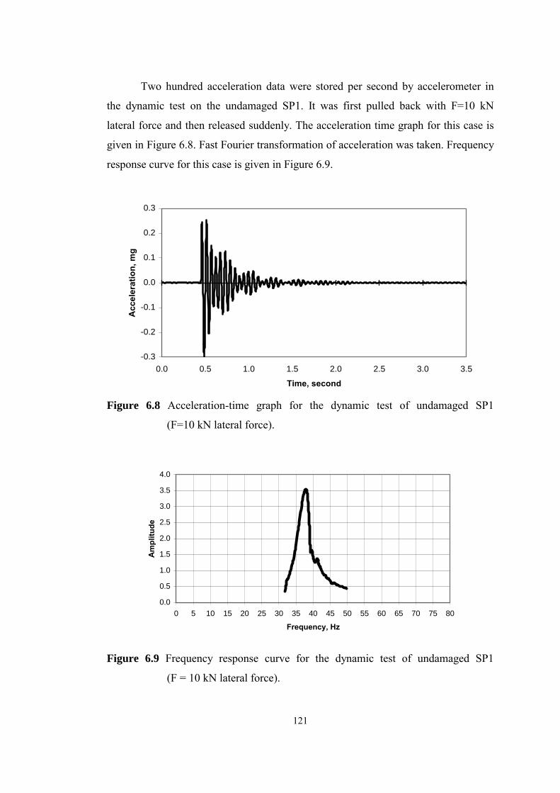
121
Two hundred acceleration data were stored per second by accelerometer in
the dynamic test on the undamaged SP1. It was first pulled back with F=10 kN
lateral force and then released suddenly. The acceleration time graph for this case is
given in Figure 6.8. Fast Fourier transformation of acceleration was taken. Frequency
response curve for this case is given in Figure 6.9.
-0.3
-0.2
-0.1
0.0
0.1
0.2
0.3
0.0 0.5 1.0 1.5 2.0 2.5 3.0 3.5
Time, second
Acc
eler
atio
n, m
g
Figure 6.8 Acceleration-time graph for the dynamic test of undamaged SP1
(F=10 kN lateral force).
0.0
0.5
1.0
1.5
2.0
2.5
3.0
3.5
4.0
0 5 10 15 20 25 30 35 40 45 50 55 60 65 70 75 80
Frequency, Hz
Am
plitu
de
Figure 6.9 Frequency response curve for the dynamic test of undamaged SP1
(F = 10 kN lateral force).
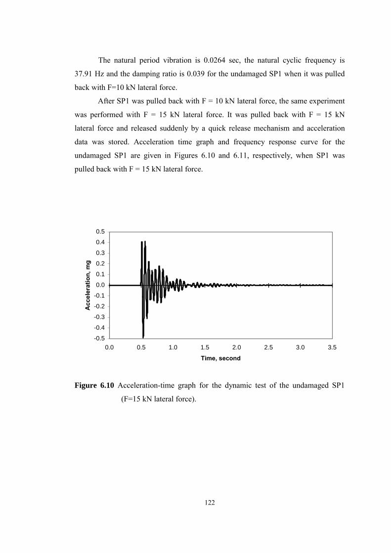
122
The natural period vibration is 0.0264 sec, the natural cyclic frequency is
37.91 Hz and the damping ratio is 0.039 for the undamaged SP1 when it was pulled
back with F=10 kN lateral force.
After SP1 was pulled back with F = 10 kN lateral force, the same experiment
was performed with F = 15 kN lateral force. It was pulled back with F = 15 kN
lateral force and released suddenly by a quick release mechanism and acceleration
data was stored. Acceleration time graph and frequency response curve for the
undamaged SP1 are given in Figures 6.10 and 6.11, respectively, when SP1 was
pulled back with F = 15 kN lateral force.
-0.5
-0.4
-0.3
-0.2
-0.1
0.0
0.1
0.2
0.3
0.4
0.5
0.0 0.5 1.0 1.5 2.0 2.5 3.0 3.5
Time, second
Acc
eler
atio
n, m
g
Figure 6.10 Acceleration-time graph for the dynamic test of the undamaged SP1
(F=15 kN lateral force).
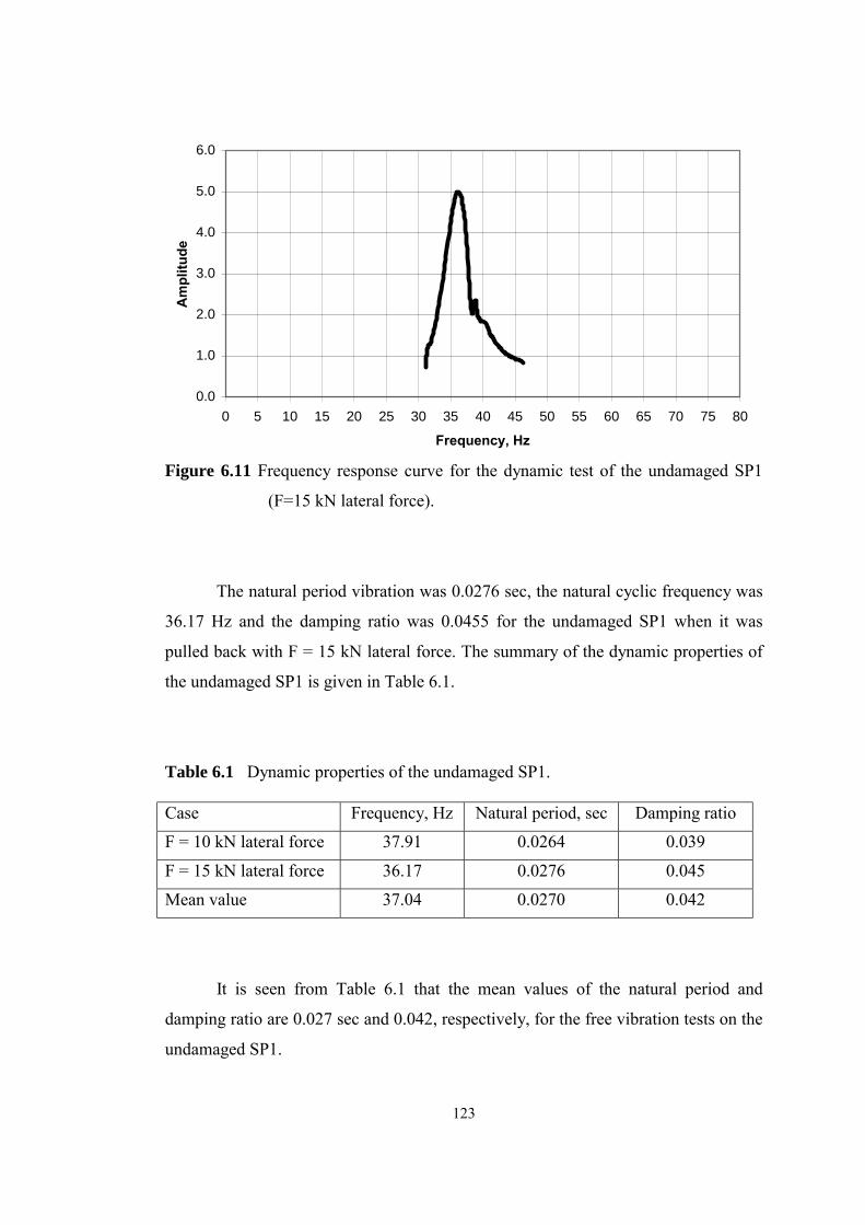
123
0.0
1.0
2.0
3.0
4.0
5.0
6.0
0 5 10 15 20 25 30 35 40 45 50 55 60 65 70 75 80
Frequency, Hz
Am
plitu
de
Figure 6.11 Frequency response curve for the dynamic test of the undamaged SP1
(F=15 kN lateral force).
The natural period vibration was 0.0276 sec, the natural cyclic frequency was
36.17 Hz and the damping ratio was 0.0455 for the undamaged SP1 when it was
pulled back with F = 15 kN lateral force. The summary of the dynamic properties of
the undamaged SP1 is given in Table 6.1.
Table 6.1 Dynamic properties of the undamaged SP1.
Case Frequency, Hz Natural period, sec Damping ratio
F = 10 kN lateral force 37.91 0.0264 0.039
F = 15 kN lateral force 36.17 0.0276 0.045
Mean value 37.04 0.0270 0.042
It is seen from Table 6.1 that the mean values of the natural period and
damping ratio are 0.027 sec and 0.042, respectively, for the free vibration tests on the
undamaged SP1.
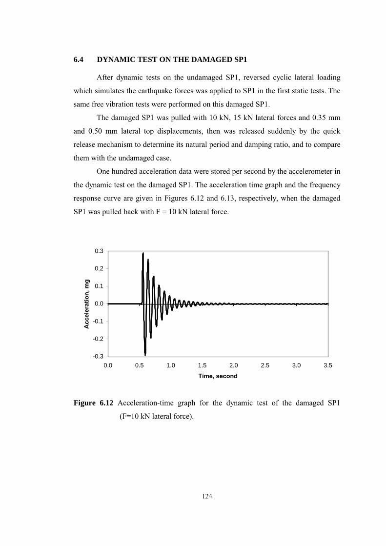
124
6.4 DYNAMIC TEST ON THE DAMAGED SP1
After dynamic tests on the undamaged SP1, reversed cyclic lateral loading
which simulates the earthquake forces was applied to SP1 in the first static tests. The
same free vibration tests were performed on this damaged SP1.
The damaged SP1 was pulled with 10 kN, 15 kN lateral forces and 0.35 mm
and 0.50 mm lateral top displacements, then was released suddenly by the quick
release mechanism to determine its natural period and damping ratio, and to compare
them with the undamaged case.
One hundred acceleration data were stored per second by the accelerometer in
the dynamic test on the damaged SP1. The acceleration time graph and the frequency
response curve are given in Figures 6.12 and 6.13, respectively, when the damaged
SP1 was pulled back with F = 10 kN lateral force.
-0.3
-0.2
-0.1
0.0
0.1
0.2
0.3
0.0 0.5 1.0 1.5 2.0 2.5 3.0 3.5
Time, second
Acc
eler
atio
n, m
g
Figure 6.12 Acceleration-time graph for the dynamic test of the damaged SP1
(F=10 kN lateral force).
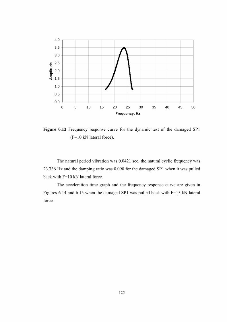
125
0.0
0.5
1.0
1.5
2.0
2.5
3.0
3.5
4.0
0 5 10 15 20 25 30 35 40 45 50
Frequency, Hz
Am
plitu
de
Figure 6.13 Frequency response curve for the dynamic test of the damaged SP1
(F=10 kN lateral force).
The natural period vibration was 0.0421 sec, the natural cyclic frequency was
23.736 Hz and the damping ratio was 0.090 for the damaged SP1 when it was pulled
back with F=10 kN lateral force.
The acceleration time graph and the frequency response curve are given in
Figures 6.14 and 6.15 when the damaged SP1 was pulled back with F=15 kN lateral
force.
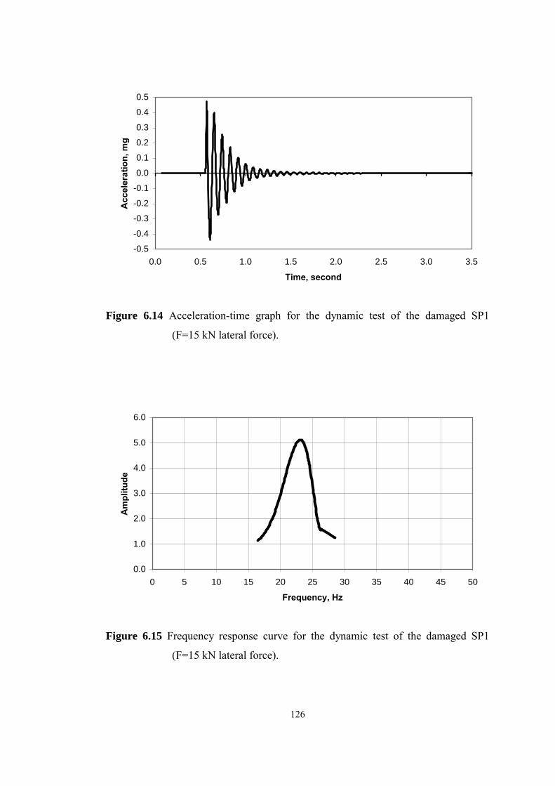
126
-0.5
-0.4
-0.3
-0.2
-0.1
0.0
0.1
0.2
0.3
0.4
0.5
0.0 0.5 1.0 1.5 2.0 2.5 3.0 3.5
Time, second
Acc
eler
atio
n, m
g
Figure 6.14 Acceleration-time graph for the dynamic test of the damaged SP1
(F=15 kN lateral force).
0.0
1.0
2.0
3.0
4.0
5.0
6.0
0 5 10 15 20 25 30 35 40 45 50
Frequency, Hz
Am
plitu
de
Figure 6.15 Frequency response curve for the dynamic test of the damaged SP1
(F=15 kN lateral force).
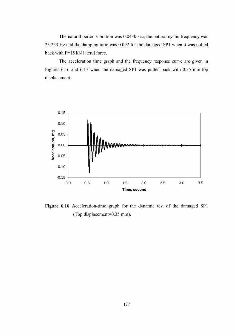
127
The natural period vibration was 0.0430 sec, the natural cyclic frequency was
23.253 Hz and the damping ratio was 0.092 for the damaged SP1 when it was pulled
back with F=15 kN lateral force.
The acceleration time graph and the frequency response curve are given in
Figures 6.16 and 6.17 when the damaged SP1 was pulled back with 0.35 mm top
displacement.
-0.15
-0.10
-0.05
0.00
0.05
0.10
0.15
0.0 0.5 1.0 1.5 2.0 2.5 3.0 3.5
Tİme, second
Acc
eler
atio
n, m
g
Figure 6.16 Acceleration-time graph for the dynamic test of the damaged SP1
(Top displacement=0.35 mm).
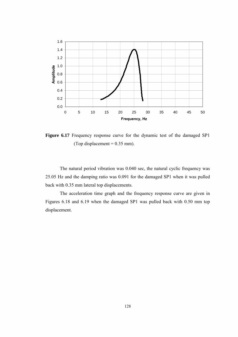
128
0.0
0.2
0.4
0.6
0.8
1.0
1.2
1.4
1.6
0 5 10 15 20 25 30 35 40 45 50
Frequency, Hz
Am
plitu
de
Figure 6.17 Frequency response curve for the dynamic test of the damaged SP1
(Top displacement = 0.35 mm).
The natural period vibration was 0.040 sec, the natural cyclic frequency was
25.05 Hz and the damping ratio was 0.091 for the damaged SP1 when it was pulled
back with 0.35 mm lateral top displacements.
The acceleration time graph and the frequency response curve are given in
Figures 6.18 and 6.19 when the damaged SP1 was pulled back with 0.50 mm top
displacement.
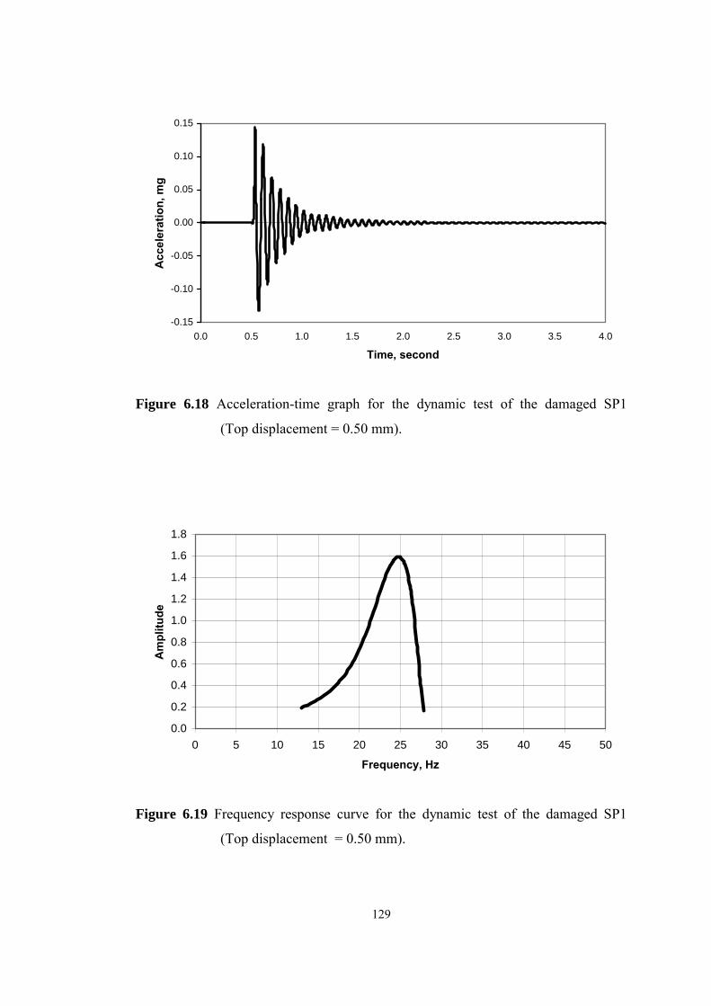
129
-0.15
-0.10
-0.05
0.00
0.05
0.10
0.15
0.0 0.5 1.0 1.5 2.0 2.5 3.0 3.5 4.0
Time, second
Acc
eler
atio
n, m
g
Figure 6.18 Acceleration-time graph for the dynamic test of the damaged SP1
(Top displacement = 0.50 mm).
0.0
0.2
0.4
0.6
0.8
1.0
1.2
1.4
1.6
1.8
0 5 10 15 20 25 30 35 40 45 50
Frequency, Hz
Am
plitu
de
Figure 6.19 Frequency response curve for the dynamic test of the damaged SP1
(Top displacement = 0.50 mm).

130
The natural period vibration was 0.0405 sec, the natural cyclic frequency was
24.657 Hz and the damping ratio was 0.093 for the damaged SP1 when it was pulled
back with 0.50 mm lateral top displacements. Table 6.2 shows the summary of the
dynamic properties of damaged SP1.
Table 6.2 Dynamic properties of damaged SP1.
Case Frequency, Hz Natural period, sec Damping ratio
F = 10 kN Lat. force 23.736 0.0421 0.0933
F = 15 kN Lat. force 23.253 0.0430 0.0917
Top disp = 0.35 mm 25.050 0.040 0.0929
Top disp = 0.50 mm 24.657 0.041 0.0957
Mean values 24.174 0.041 0.0934
The free vibration tests on the undamaged SP1 show that the mean values of
the natural period and damping ratio are 0.027 sec and 0.042, respectively. In the free
vibration tests of the damaged SP1 the mean values of the natural period and
damping ratio were 0.041 and 0.0934. The natural period of free vibration increases
0.041 / 0.027 = 1.518 times and damping ratios increase 0.093 / 0.042 = 2.224 times
from the undamaged case to the damaged case for SP1.
6.5 DYNAMIC TEST ON THE UNDAMAGED SP2
SP2 was pulled along the long dimension and released suddenly so that the
acceleration, calculated period and damping ratio of SP2 were along that dimension.
Figure 6.20 shows the details of the test setup, loading system and instrumentation
for the dynamic test of SP2. As can be seen in Figure 6.20, SP2 was pulled back with
the help of a hydraulic jack and the lateral load was measured by load cell. SP2 was
first pulled back with F = 10 kN lateral force and then released suddenly. Two
hundred acceleration data were stored per second by the accelerometer in the
dynamic tests of the undamaged SP2 as was done for the undamaged SP1. The
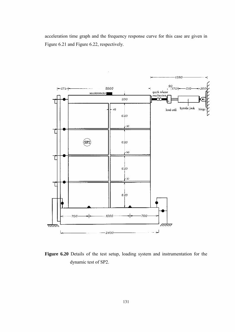
131
acceleration time graph and the frequency response curve for this case are given in
Figure 6.21 and Figure 6.22, respectively.
Figure 6.20 Details of the test setup, loading system and instrumentation for the
dynamic test of SP2.
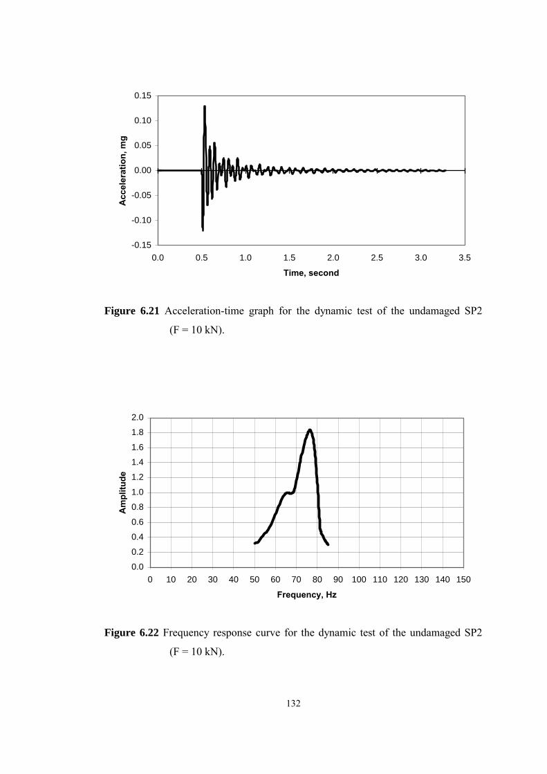
132
-0.15
-0.10
-0.05
0.00
0.05
0.10
0.15
0.0 0.5 1.0 1.5 2.0 2.5 3.0 3.5
Time, second
Acc
eler
atio
n, m
g
Figure 6.21 Acceleration-time graph for the dynamic test of the undamaged SP2
(F = 10 kN).
0.0
0.2
0.4
0.6
0.8
1.0
1.2
1.4
1.6
1.8
2.0
0 10 20 30 40 50 60 70 80 90 100 110 120 130 140 150
Frequency, Hz
Am
plitu
de
Figure 6.22 Frequency response curve for the dynamic test of the undamaged SP2
(F = 10 kN).

133
The natural period vibration was 0.013 sec, the natural cyclic frequency was
76.71 Hz and the damping ratio was 0.055 for the undamaged SP2 when it was
pulled back with F = 10 kN lateral force.
After SP2 was pulled back with F = 10 kN lateral force, it was pulled back
with F= 15 kN lateral force and released suddenly by the quick release mechanism
and acceleration data were stored. Acceleration time graph and frequency response
curve for the undamaged SP2 are given in Figures 6.23 and 6.24, respectively.
-0.3
-0.2
-0.1
0.0
0.1
0.2
0.3
0.0 0.5 1.0 1.5 2.0 2.5 3.0 3.5
Time, second
Acc
eler
atio
n, m
g
Figure 6.23 Acceleration-time graph for the dynamic test of the undamaged SP2
(F=15 kN).

134
0.0
0.5
1.0
1.5
2.0
2.5
3.0
3.5
4.0
0 10 20 30 40 50 60 70 80 90 100 110 120 130 140 150
Frequency, Hz
Am
plitu
de
Figure 6.24 Frequency response curve for the dynamic test of the undamaged SP2
(F = 15 kN).
The natural period vibration was 0.0142 sec, the natural cyclic frequency was
70.45 Hz and the damping ratio was 0.092 for the undamaged SP2 when it was
pulled back with F = 15 kN lateral force.
The acceleration time graph and the frequency response curve are given in
Figures 6.25 and 6.26 when the undamaged SP2 was pulled back with F = 20 kN
lateral force.

135
-0.4
-0.3
-0.2
-0.1
0.0
0.1
0.2
0.3
0.4
0.5
0.0 0.5 1.0 1.5 2.0 2.5 3.0 3.5 4.0
Time, second
Acc
eler
atio
n, m
g
Figure 6.25 Acceleration-time graph for the dynamic test of the undamaged SP2
(F = 20 kN).
0
1
2
3
4
5
6
7
0 10 20 30 40 50 60 70 80 90 100 110 120 130 140 150
Frequency, Hz
Am
plitu
de
Figure 6.26 Frequency response curve for the dynamic test of the undamaged SP2
(F = 20 kN).
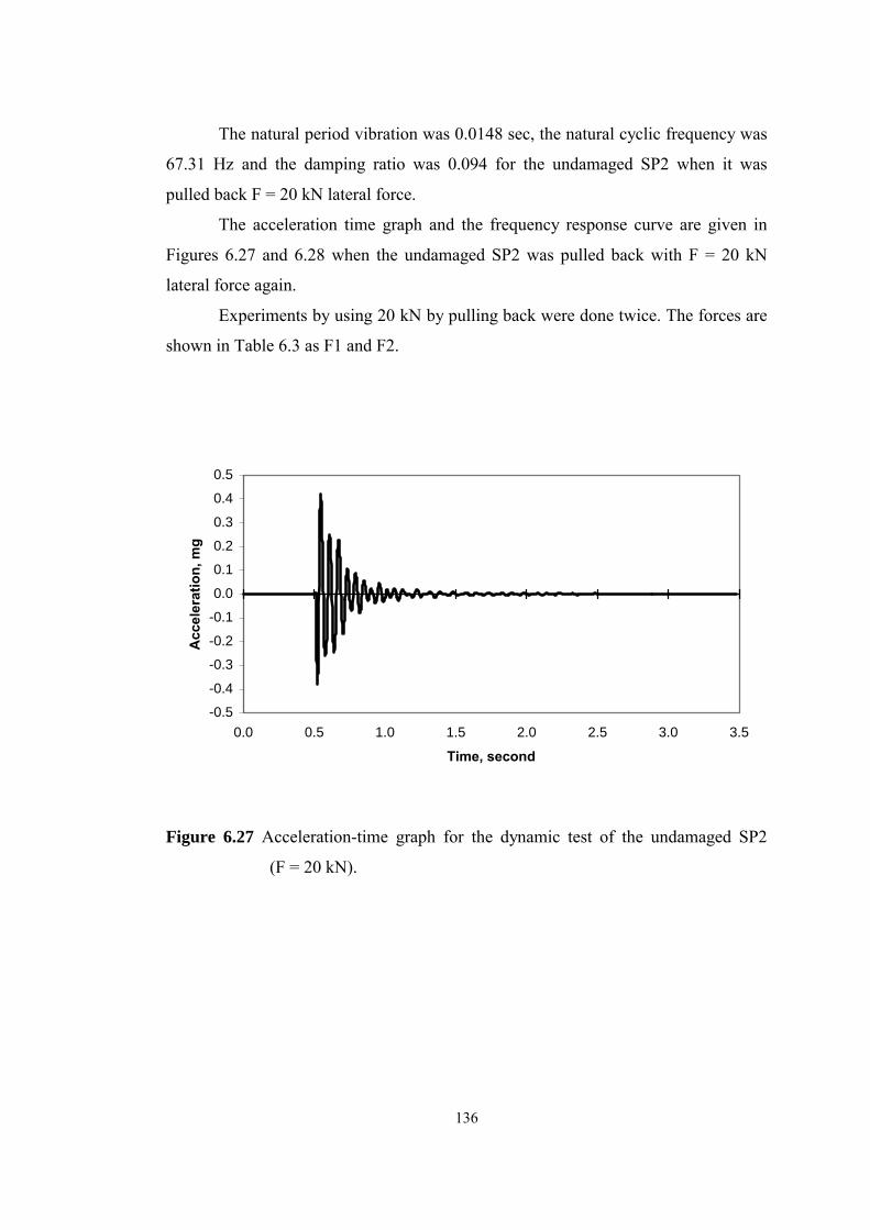
136
The natural period vibration was 0.0148 sec, the natural cyclic frequency was
67.31 Hz and the damping ratio was 0.094 for the undamaged SP2 when it was
pulled back F = 20 kN lateral force.
The acceleration time graph and the frequency response curve are given in
Figures 6.27 and 6.28 when the undamaged SP2 was pulled back with F = 20 kN
lateral force again.
Experiments by using 20 kN by pulling back were done twice. The forces are
shown in Table 6.3 as F1 and F2.
-0.5
-0.4
-0.3
-0.2
-0.1
0.0
0.1
0.2
0.3
0.4
0.5
0.0 0.5 1.0 1.5 2.0 2.5 3.0 3.5
Time, second
Acc
eler
atio
n, m
g
Figure 6.27 Acceleration-time graph for the dynamic test of the undamaged SP2
(F = 20 kN).
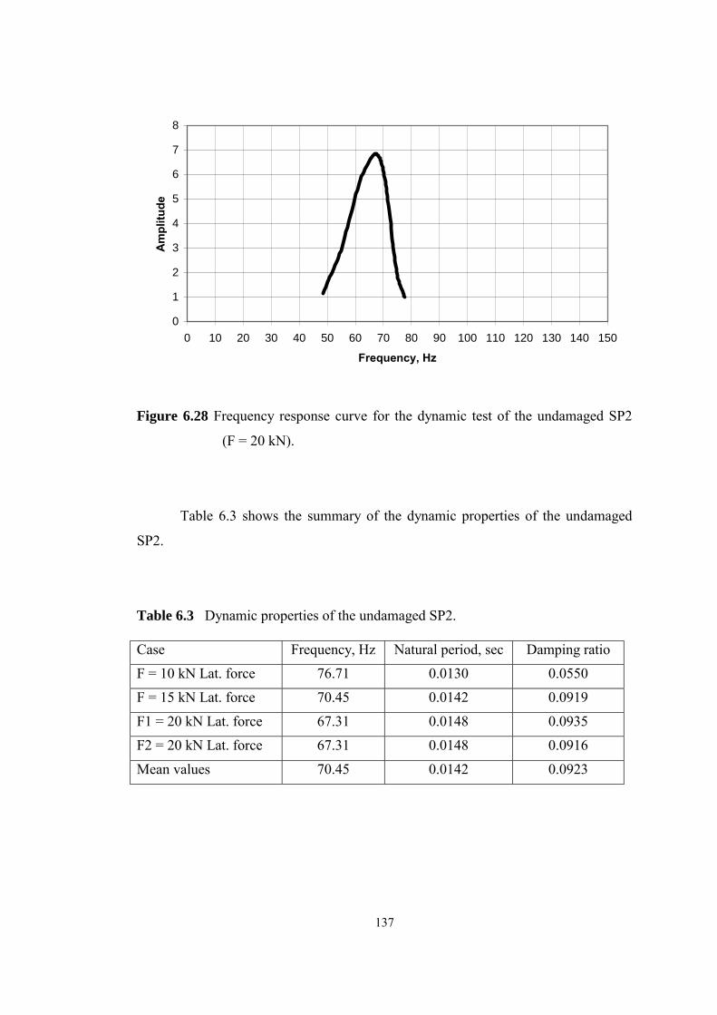
137
0
1
2
3
4
5
6
7
8
0 10 20 30 40 50 60 70 80 90 100 110 120 130 140 150
Frequency, Hz
Am
plitu
de
Figure 6.28 Frequency response curve for the dynamic test of the undamaged SP2
(F = 20 kN).
Table 6.3 shows the summary of the dynamic properties of the undamaged
SP2.
Table 6.3 Dynamic properties of the undamaged SP2.
Case Frequency, Hz Natural period, sec Damping ratio
F = 10 kN Lat. force 76.71 0.0130 0.0550
F = 15 kN Lat. force 70.45 0.0142 0.0919
F1 = 20 kN Lat. force 67.31 0.0148 0.0935
F2 = 20 kN Lat. force 67.31 0.0148 0.0916
Mean values 70.45 0.0142 0.0923
138
6.6 DYNAMIC TEST ON THE DAMAGED SP2
After the dynamic tests on the undamaged SP2 were completed, reversed
cyclic lateral loading which simulates the earthquake forces was applied to SP2 in
the first static tests. The same free vibration tests were performed on this damaged
SP2.
The damaged SP2 was pulled with 10 kN, 15 kN and 20 kN lateral forces and
was released suddenly by the quick release mechanism to determine its natural
period and damping ratio and to compare them with the undamaged case.
The acceleration time graph and the frequency response curve are given in
Figures 6.29 and 6.30 when the damaged SP2 was pulled back with F = 10 kN lateral
force.
-0.3
-0.2
-0.1
0.0
0.1
0.2
0.3
0.0 0.5 1.0 1.5 2.0 2.5 3.0 3.5
Time, second
Acc
eler
atio
n, m
g
Figure 6.29 Acceleration-time graph for the dynamic test of the damaged SP2
(F = 10 kN).
139
0.0
0.5
1.0
1.5
2.0
2.5
3.0
3.5
0 10 20 30 40 50 60 70 80 90 100 110 120 130 140 150
Frequency, Hz
Am
plitu
de
Figure 6.30 Frequency response curve for the dynamic test of the damaged SP2
(F = 10 kN).
The natural period vibration was 0.0145 sec, the natural cyclic frequency was
68.885 Hz and the damping ratio was 0.117 for the undamaged SP2 when it was
pulled back F= 10 kN lateral force.
The acceleration time graph and the frequency response curve are given in
Figures 6.31 and 6.32 when the undamaged SP2 was pulled back with F = 15 kN
lateral force.
140
-0.3
-0.2
-0.1
0.0
0.1
0.2
0.3
0.0 0.5 1.0 1.5 2.0 2.5 3.0 3.5
Time, second
Acc
eler
atio
n, m
g
Figure 6.31 Acceleration-time graph for the dynamic test of the damaged SP2
(F = 15 kN)
0.0
0.5
1.0
1.5
2.0
2.5
3.0
3.5
0 10 20 30 40 50 60 70 80 90 100 110 120 130 140 150
Frequency, Hz
Am
plitu
de
Figure 6.32 Frequency response curve for the dynamic test of the damaged SP2
(F = 15 kN).

141
The natural period vibration was 0.0168 sec, the natural cyclic frequency was
59.7 Hz and the damping ratio was 0.117 for the undamaged SP2 when it was pulled
back F = 15 kN lateral force.
The acceleration time graph and the frequency response curve are given in
Figures 6.33 and 6.34 when the undamaged SP2 was pulled back with F = 20 kN
lateral force.
-0.5
-0.4
-0.3
-0.2
-0.1
0.0
0.1
0.2
0.3
0.4
0.5
0.0 0.5 1.0 1.5 2.0 2.5 3.0 3.5
Time, second
Acc
eler
atio
n, m
g
Figure 6.33 Acceleration-time graph for the dynamic test of the damaged SP2
(F = 20 kN).
142
0
1
2
3
4
5
6
7
0 10 20 30 40 50 60 70 80 90 100 110 120 130 140 150
Frequency, Hz
Am
plitu
de
Figure 6.34 Frequency response curve for the dynamic test of the damaged SP2
(F = 20 kN).
The natural period vibration was 0.0177 sec, the natural cyclic frequency was
56.534 Hz and the damping ratio was 0.112 for the undamaged SP2 when it was
pulled back F= 20 kN lateral force.
The acceleration time graph and the frequency response curve are given in
Figures 6.35 and 6.36 when the damaged SP2 was pulled back with F = 20 kN lateral
force.
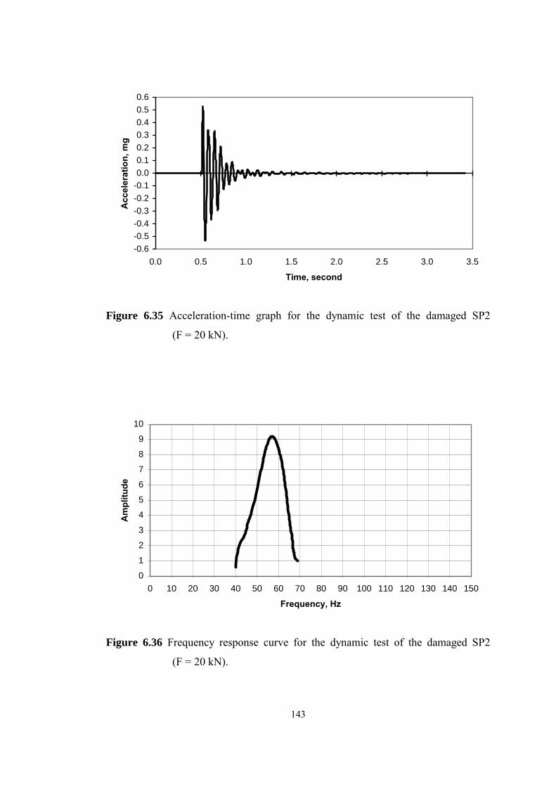
143
-0.6-0.5-0.4-0.3-0.2-0.10.00.10.20.30.40.50.6
0.0 0.5 1.0 1.5 2.0 2.5 3.0 3.5
Time, second
Acc
eler
atio
n, m
g
Figure 6.35 Acceleration-time graph for the dynamic test of the damaged SP2
(F = 20 kN).
0
1
2
3
4
5
6
7
8
9
10
0 10 20 30 40 50 60 70 80 90 100 110 120 130 140 150
Frequency, Hz
Am
plitu
de
Figure 6.36 Frequency response curve for the dynamic test of the damaged SP2
(F = 20 kN).
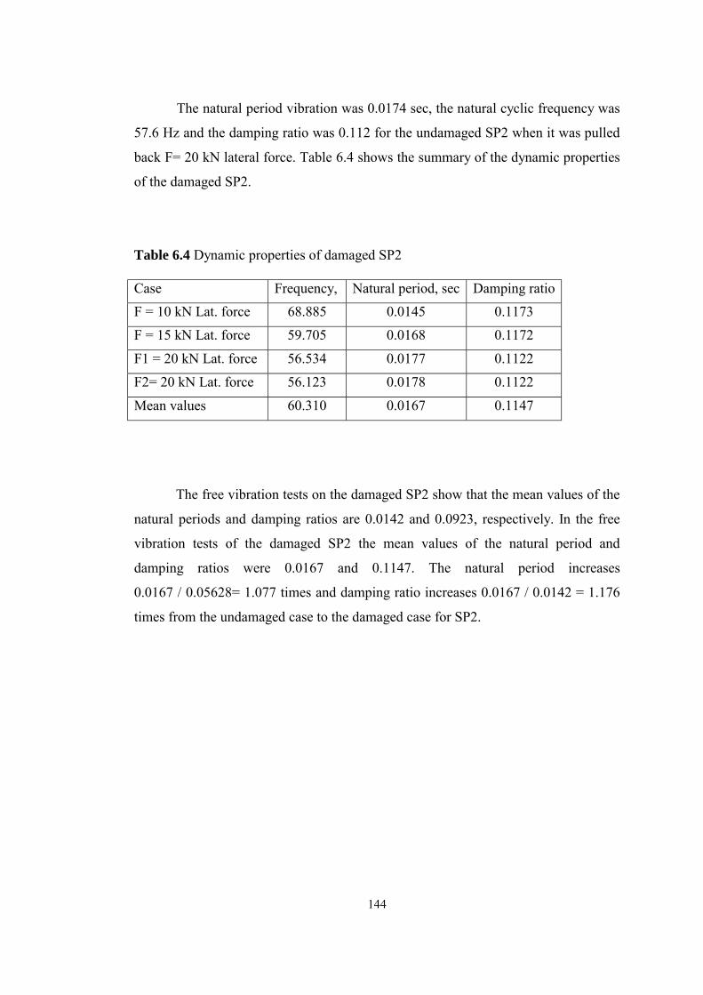
144
The natural period vibration was 0.0174 sec, the natural cyclic frequency was
57.6 Hz and the damping ratio was 0.112 for the undamaged SP2 when it was pulled
back F= 20 kN lateral force. Table 6.4 shows the summary of the dynamic properties
of the damaged SP2.
Table 6.4 Dynamic properties of damaged SP2
Case Frequency, Natural period, sec Damping ratio F = 10 kN Lat. force 68.885 0.0145 0.1173
F = 15 kN Lat. force 59.705 0.0168 0.1172
F1 = 20 kN Lat. force 56.534 0.0177 0.1122
F2= 20 kN Lat. force 56.123 0.0178 0.1122
Mean values 60.310 0.0167 0.1147
The free vibration tests on the damaged SP2 show that the mean values of the
natural periods and damping ratios are 0.0142 and 0.0923, respectively. In the free
vibration tests of the damaged SP2 the mean values of the natural period and
damping ratios were 0.0167 and 0.1147. The natural period increases
0.0167 / 0.05628= 1.077 times and damping ratio increases 0.0167 / 0.0142 = 1.176
times from the undamaged case to the damaged case for SP2.

145
6.7 COMPARISON OF THE DYNAMIC TEST RESULTS
Table 6.5 shows the summary of dynamic properties of the test specimens. In
the first dynamic tests on SP1 the natural period and damping ratio are found to be
0.0270 sec and 0.039, respectively, for the uncracked case. The second dynamic tests
on SP1 show that the natural period and damping ratio increase up to 0.041 sec and
0.0935, respectively, for the cracked case. The natural period increases
0.041 / 0.027 = 1.518 times and damping ratio increases 0.0935 / 0.039 = 2.397 times
from the uncracked case to the cracked case for SP1.
For SP2 the natural period and the damping ratio in the first dynamic test are
found to be 0.0142 sec and 0.0934, respectively. The natural period and the damping
ratio of SP2 in the second dynamic tests increase up to 0.0167 sec and 0.1125,
respectively, for the cracked case. The natural period and the damping ratio increase
0.0167 / 0.0142 = 1.176 and 0.1125 / 0.0934 = 1.2045 times, respectively, from the
first dynamic test to the second dynamic test on SP2.
The increment of the natural period and the damping ratios from the first
dynamic test to the second dynamic test on SP1 is considerable, but it is negligible
for SP2. It is seen from Table 6.5 that after cracking the natural period of vibration
increases.
Table 6.5 Dynamic properties of the panel form test specimens.
CASE Natural period Damping ratio
1st dynamic test on SP1 0.0270 0.0390
2nd dynamic test on SP1 0.0410 0.0935
1st dynamic test on SP2 0.0142 0.0934
2nd dynamic test on SP2 0.0167 0.1125
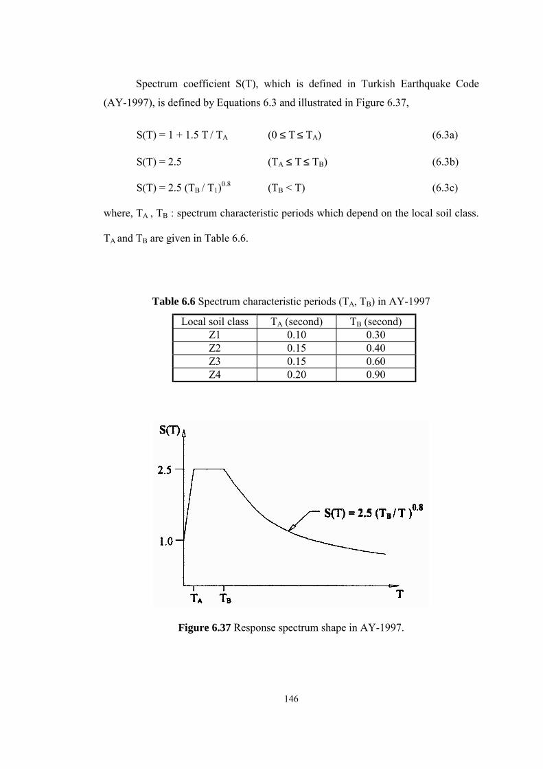
146
Spectrum coefficient S(T), which is defined in Turkish Earthquake Code
(AY-1997), is defined by Equations 6.3 and illustrated in Figure 6.37,
S(T) = 1 + 1.5 T / TA (0 ≤ T ≤ TA) (6.3a)
S(T) = 2.5 (TA ≤ T ≤ TB) (6.3b)
S(T) = 2.5 (TB / T1)0.8 (TB < T) (6.3c)
where, TA , TB : spectrum characteristic periods which depend on the local soil class.
TA and TB are given in Table 6.6.
Table 6.6 Spectrum characteristic periods (TA, TB) in AY-1997
Local soil class TA (second) TB (second) Z1 0.10 0.30 Z2 0.15 0.40 Z3 0.15 0.60 Z4 0.20 0.90
Figure 6.37 Response spectrum shape in AY-1997.

147
Tunnel form buildings are very stiff structures, therefore natural period of
vibrations of the tunnel form structures are generally smaller than 0.10 seconds. It is
seen from the response spectrum shape that after cracking the spectrum values of the
tunnel form buildings increase due to increasing of the natural period of vibration.
Earthquake forces on the tunnel form buildings also increase after cracking of the
wall section. It can be concluded that a tunnel form building is not safe, after
concrete cracking, during an earthquake.
6.8 EIGENVALUE ANALYSIS FOR THE PANEL FORM TEST
SPECIMENS
Mode superposition analysis was performed on the test specimens to
determine the frequencies, periods, mode shapes, modal displacements and mass
participation ratios. Test specimens were modeled by using the finite element
techniques and wide-column-frame analogy. A general-purpose finite element
program called SAP2000 was used.
6.8.1 Finite Element Modeling
In this study shear walls and slabs are modeled by using a rectangular mesh
of isotropic shell elements of four joint formulations, which combine the membrane
and plate-bending behavior. This shell element activates all six degrees of freedom at
each of its connected joints. Each shell element has its own local coordinate system
for defining material properties, mass, loads, and for interpreting output.
In order to satisfy adequate accuracy for the test specimens, the walls are
divided into elements having dimensions of 158.75 mm × 200 mm and the floor
slabs are divided into elements having dimensions of 168 mm × 200 mm, as shown
in Figure 6.38. The result of the eigenvalue analysis by using finite element method
is given in Table 6.7. Fundamental periods of vibration of the specimens for 1st, 2nd,
and 3rd modes are given in Figures 6.39, 6.40 and 6.41, respectively.

148
Table 6.7 The result of the eigenvalue analysis for finite element modeling
Mode Number
Frequency (cycles/sec)
Period (second)
Mode Shape
1 37.593 0.0266 Translation along short dimension 2 45.871 0.0218 Torsional motion 3 61.350 0.0163 Translation along long dimension
Figure 6.38 Finite Element Modeling of the panel form test specimens.
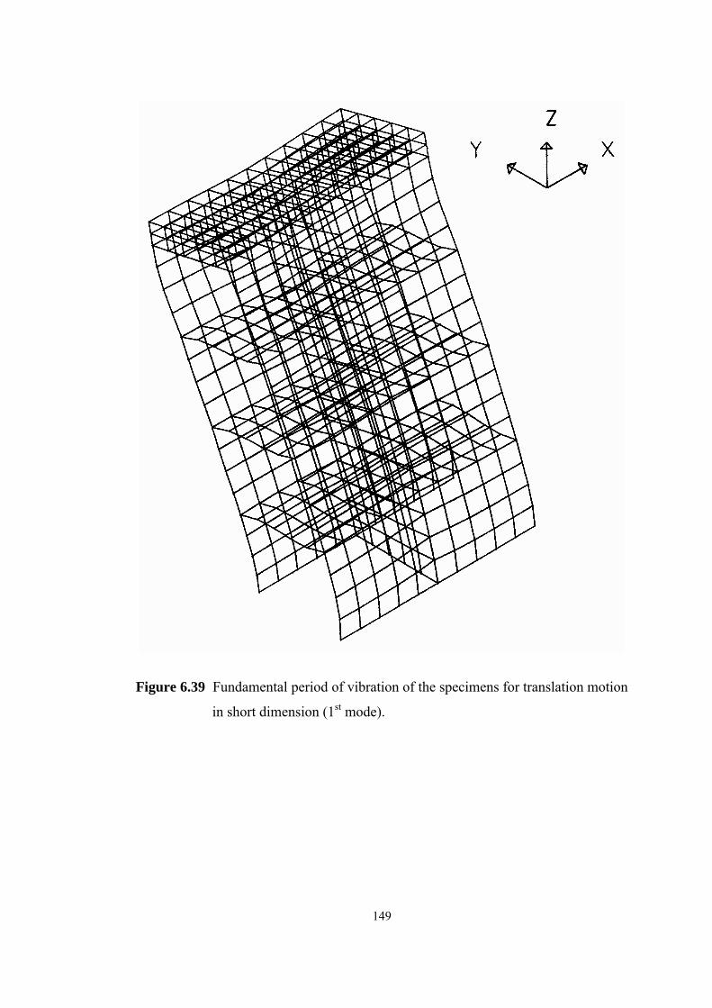
149
Figure 6.39 Fundamental period of vibration of the specimens for translation motion
in short dimension (1st mode).
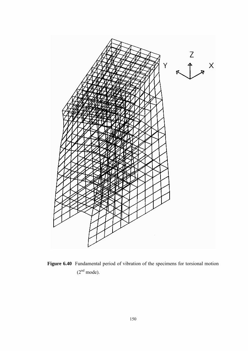
150
Figure 6.40 Fundamental period of vibration of the specimens for torsional motion
(2nd mode).
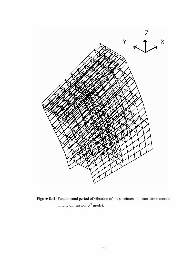
151
Figure 6.41 Fundamental period of vibration of the specimens for translation motion
in long dimension (3rd mode).
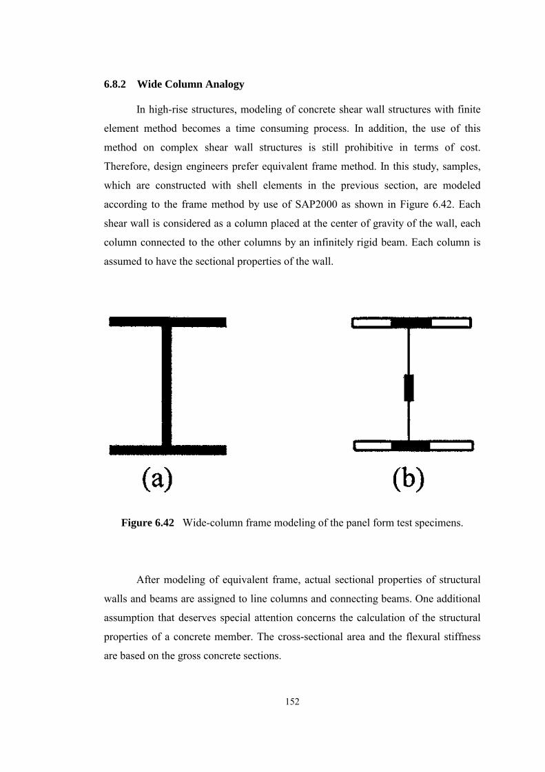
152
6.8.2 Wide Column Analogy
In high-rise structures, modeling of concrete shear wall structures with finite
element method becomes a time consuming process. In addition, the use of this
method on complex shear wall structures is still prohibitive in terms of cost.
Therefore, design engineers prefer equivalent frame method. In this study, samples,
which are constructed with shell elements in the previous section, are modeled
according to the frame method by use of SAP2000 as shown in Figure 6.42. Each
shear wall is considered as a column placed at the center of gravity of the wall, each
column connected to the other columns by an infinitely rigid beam. Each column is
assumed to have the sectional properties of the wall.
Figure 6.42 Wide-column frame modeling of the panel form test specimens.
After modeling of equivalent frame, actual sectional properties of structural
walls and beams are assigned to line columns and connecting beams. One additional
assumption that deserves special attention concerns the calculation of the structural
properties of a concrete member. The cross-sectional area and the flexural stiffness
are based on the gross concrete sections.
153
Theoretically, rigid arms are assumed to have infinite moments of inertia and
sectional area. However, extremely large areas can create errors or large inaccuracies
in the results. Therefore, although the program used allows infinite rigid arms,
perfect rigidity is not applied to avoid unexpected errors. Area and moments of
inertia of the rigid arms are determined according to the following formulas proposed
(Mattachoine, 1991);
Ae = 100 ×(e/f)
Ie / If = 100 × (e/f)3 + 300 (e/f)2 + 300 (e/f)
where,
e : length of stiff-ended section
f : half length of connected beam
Ae : area of stiff-ended section
Ie : moments of inertia of stiff ended section
Af : area of connecting beam
If : moments of inertia of connecting beam
Because of their inherent economy, “Flat Slabs” are widely used in shear wall
structures, in particular apartment buildings. In addition to carrying the floor loads,
they also act as rigid horizontal diaphragms. Rigid-floor behavior is modeled by
generating a joint in the plane of the diaphragm. Translational mass values and
rotational mass value around out-of-plane axis are assigned to the master joints
according to the procedure stated by the structure analysis program.
The result of the eigenvalue analysis by using wide column frame analogy is
given in Table 6.8.
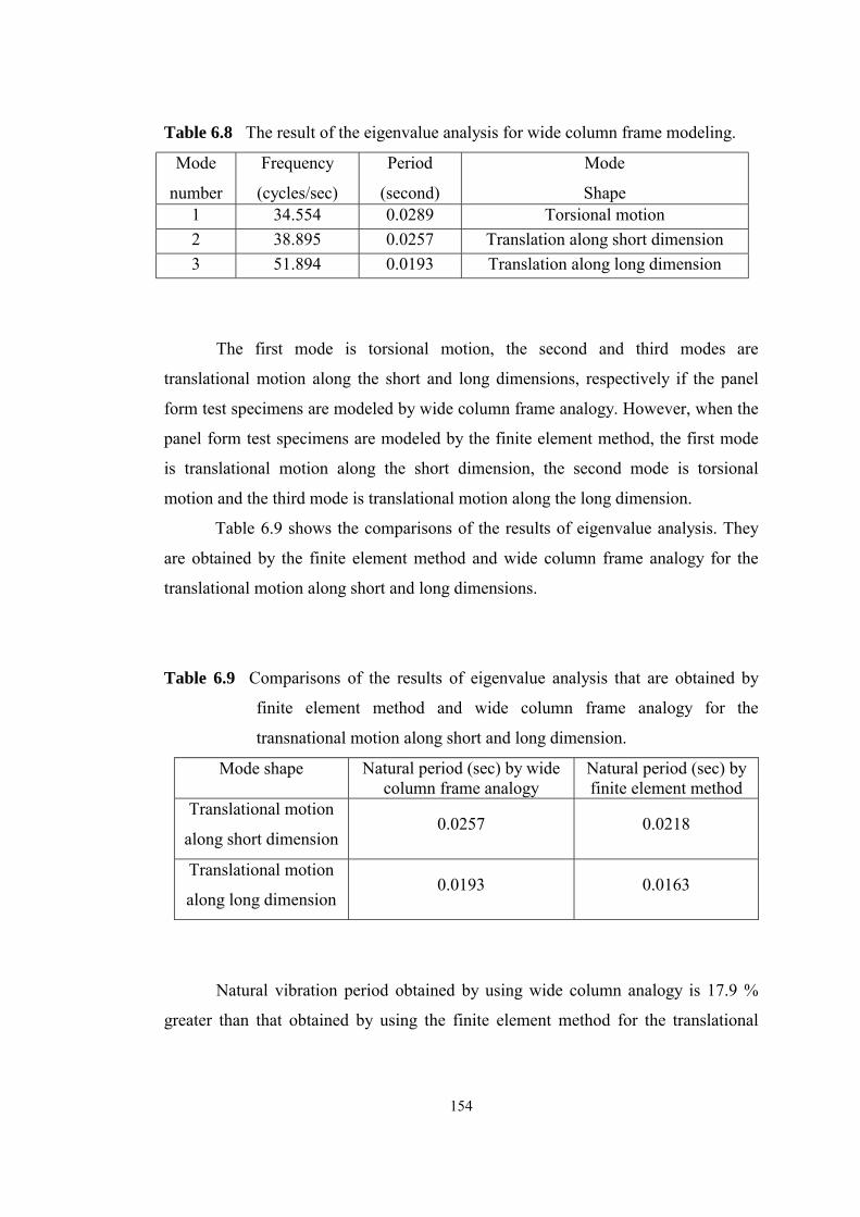
154
Table 6.8 The result of the eigenvalue analysis for wide column frame modeling.
Mode
number
Frequency
(cycles/sec)
Period
(second)
Mode
Shape 1 34.554 0.0289 Torsional motion 2 38.895 0.0257 Translation along short dimension 3 51.894 0.0193 Translation along long dimension
The first mode is torsional motion, the second and third modes are
translational motion along the short and long dimensions, respectively if the panel
form test specimens are modeled by wide column frame analogy. However, when the
panel form test specimens are modeled by the finite element method, the first mode
is translational motion along the short dimension, the second mode is torsional
motion and the third mode is translational motion along the long dimension.
Table 6.9 shows the comparisons of the results of eigenvalue analysis. They
are obtained by the finite element method and wide column frame analogy for the
translational motion along short and long dimensions.
Table 6.9 Comparisons of the results of eigenvalue analysis that are obtained by
finite element method and wide column frame analogy for the
transnational motion along short and long dimension.
Mode shape Natural period (sec) by wide column frame analogy
Natural period (sec) by finite element method
Translational motion
along short dimension 0.0257 0.0218
Translational motion
along long dimension 0.0193 0.0163
Natural vibration period obtained by using wide column analogy is 17.9 %
greater than that obtained by using the finite element method for the translational
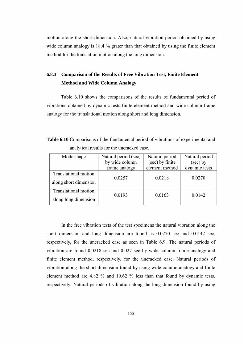
155
motion along the short dimension. Also, natural vibration period obtained by using
wide column analogy is 18.4 % grater than that obtained by using the finite element
method for the translation motion along the long dimension.
6.8.3 Comparison of the Results of Free Vibration Test, Finite Element
Method and Wide Column Analogy
Table 6.10 shows the comparisons of the results of fundamental period of
vibrations obtained by dynamic tests finite element method and wide column frame
analogy for the translational motion along short and long dimension.
Table 6.10 Comparisons of the fundamental period of vibrations of experimental and
analytical results for the uncracked case.
Mode shape Natural period (sec) by wide column frame analogy
Natural period (sec) by finite
element method
Natural period (sec) by
dynamic tests Translational motion
along short dimension 0.0257 0.0218 0.0270
Translational motion
along long dimension 0.0193 0.0163 0.0142
In the free vibration tests of the test specimens the natural vibration along the
short dimension and long dimension are found as 0.0270 sec and 0.0142 sec,
respectively, for the uncracked case as seen in Table 6.9. The natural periods of
vibration are found 0.0218 sec and 0.027 sec by wide column frame analogy and
finite element method, respectively, for the uncracked case. Natural periods of
vibration along the short dimension found by using wide column analogy and finite
element method are 4.82 % and 19.62 % less than that found by dynamic tests,
respectively. Natural periods of vibration along the long dimension found by using
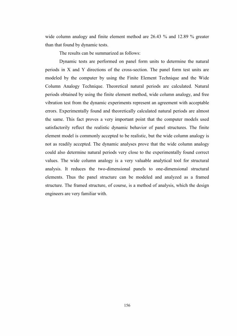
156
wide column analogy and finite element method are 26.43 % and 12.89 % greater
than that found by dynamic tests.
The results can be summarized as follows:
Dynamic tests are performed on panel form units to determine the natural
periods in X and Y directions of the cross-section. The panel form test units are
modeled by the computer by using the Finite Element Technique and the Wide
Column Analogy Technique. Theoretical natural periods are calculated. Natural
periods obtained by using the finite element method, wide column analogy, and free
vibration test from the dynamic experiments represent an agreement with acceptable
errors. Experimentally found and theoretically calculated natural periods are almost
the same. This fact proves a very important point that the computer models used
satisfactorily reflect the realistic dynamic behavior of panel structures. The finite
element model is commonly accepted to be realistic, but the wide column analogy is
not as readily accepted. The dynamic analyses prove that the wide column analogy
could also determine natural periods very close to the experimentally found correct
values. The wide column analogy is a very valuable analytical tool for structural
analysis. It reduces the two-dimensional panels to one-dimensional structural
elements. Thus the panel structure can be modeled and analyzed as a framed
structure. The framed structure, of course, is a method of analysis, which the design
engineers are very familiar with.

157
CHAPTER 7
A MOMENT-CURVATURE PROGRAM FOR STRUCTURAL
WALLS
7.1 INTRODUCTION
Shear wall cross-sectional dimensions, reinforcement detailing and the
location of the confined sections are different those in actual columns and beams.
Therefore some problems can arise in deriving moment-curvature relationships for
shear walls. Available computer programs that are used to obtain the moment-
curvature diagram have limited capacity in the modeling of reinforced concrete
sections for shear walls. For example the available moment-curvature program
Response (2000), which, is available on the web address of
(http://www.ecf.utoronto.ca/~bentz/r2k.htm) does not have an option for the
modeling of confined concrete. Therefore, the moment-curvature response of
structural walls, which have confined end regions, cannot be predicted by using this
program. For this purpose the computer program Waller2002, which includes the
effects of steel strain hardening, confinement of concrete, and tension strength of
concrete in deriving the moment-curvature relationship of shear walls, has been
developed. The basic assumptions and algorithms of this program have been
explained in detail. The results given by the Waller2002 for two cases where the
longitudinal boundary reinforcement is not confined using transverse reinforcement
are compared with those obtained from Response2000. Four shear wall cases were
investigated by changing the longitudinal and transverse reinforcement ratio in the
boundary element.
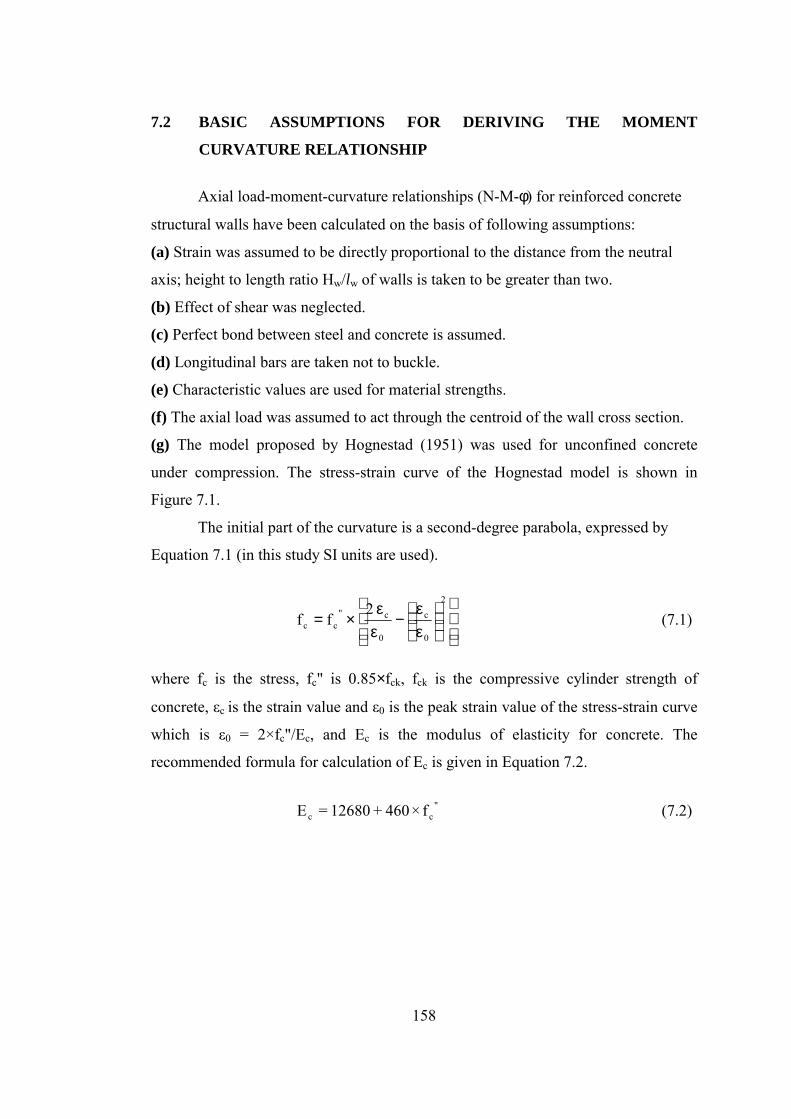
158
7.2 BASIC ASSUMPTIONS FOR DERIVING THE MOMENT
CURVATURE RELATIONSHIP
Axial load-moment-curvature relationships (N-M-φ) for reinforced concrete
structural walls have been calculated on the basis of following assumptions:
(a) Strain was assumed to be directly proportional to the distance from the neutral
axis; height to length ratio Hw/lw of walls is taken to be greater than two.
(b) Effect of shear was neglected.
(c) Perfect bond between steel and concrete is assumed.
(d) Longitudinal bars are taken not to buckle.
(e) Characteristic values are used for material strengths.
(f) The axial load was assumed to act through the centroid of the wall cross section.
(g) The model proposed by Hognestad (1951) was used for unconfined concrete
under compression. The stress-strain curve of the Hognestad model is shown in
Figure 7.1.
The initial part of the curvature is a second-degree parabola, expressed by
Equation 7.1 (in this study SI units are used).
εε
−εε
×=2
0
c
0
c"cc
2ff
(7.1)
where fc is the stress, fc" is 0.85×fck, fck is the compressive cylinder strength of
concrete, εc is the strain value and ε0 is the peak strain value of the stress-strain curve
which is ε0 = 2×fc"/Ec, and Ec is the modulus of elasticity for concrete. The
recommended formula for calculation of Ec is given in Equation 7.2.
"
cc f×460+12680=E (7.2)
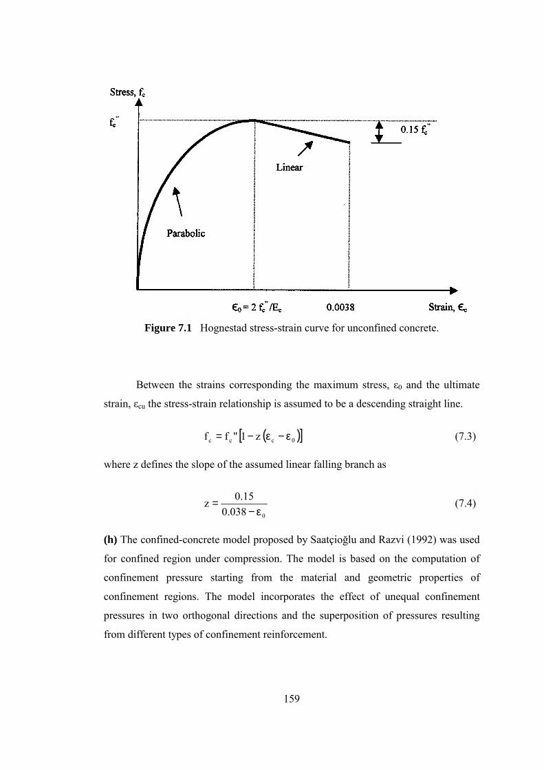
159
Figure 7.1 Hognestad stress-strain curve for unconfined concrete.
Between the strains corresponding the maximum stress, ε0 and the ultimate
strain, εcu the stress-strain relationship is assumed to be a descending straight line.
( )[ ]0ccc z1 "ff ε−ε−= (7.3) where z defines the slope of the assumed linear falling branch as
0038.0
15.0zε−
= (7.4)
(h) The confined-concrete model proposed by Saatçioğlu and Razvi (1992) was used
for confined region under compression. The model is based on the computation of
confinement pressure starting from the material and geometric properties of
confinement regions. The model incorporates the effect of unequal confinement
pressures in two orthogonal directions and the superposition of pressures resulting
from different types of confinement reinforcement.

160
Figure 7.2 illustrates the stress-strain curve of the Saatçioğlu and Razvi
(1992) model for confined concrete. The model consists of a parabolic ascending
branch, followed by a linear descending segment and a residual strength. Equation
7.5 describes the ascending branch of the Saatçioğlu and Razvi model for confined
concrete.
'f2'ff cc
)K21/(12
coc
c
coc
cccc ≤
εε−
εε=
+
(7.5)
Figure 7.2 Stress-Strain curve of the Saatcioğlu and Ravzi model.
where fc is the stress, εc is the strain, fcc' is the confined concrete strength and εcoc is
the corresponding strain and K is a constant calculated considering the hoop spacing,
spacing of laterally supported longitudinal reinforcement, equivalent uniform
pressure, strength of unconfined concrete and the width and depth of the confined
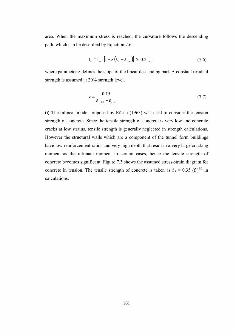
161
area. When the maximum stress is reached, the curvature follows the descending
path, which can be described by Equation 7.6.
( )[ ] 'f 2.0 z1 f f cccocc
'ccc ≥ε−ε−= (7.6)
where parameter z defines the slope of the linear descending part. A constant residual
strength is assumed at 20% strength level.
coc85cc
15.0zε−ε
= (7.7)
(i) The bilinear model proposed by Rüsch (1963) was used to consider the tension
strength of concrete. Since the tensile strength of concrete is very low and concrete
cracks at low strains, tensile strength is generally neglected in strength calculations.
However the structural walls which are a component of the tunnel form buildings
have low reinforcement ratios and very high depth that result in a very large cracking
moment as the ultimate moment in certain cases, hence the tensile strength of
concrete becomes significant. Figure 7.3 shows the assumed stress-strain diagram for
concrete in tension. The tensile strength of concrete is taken as fct = 0.35 (fc)1/2 in
calculations.
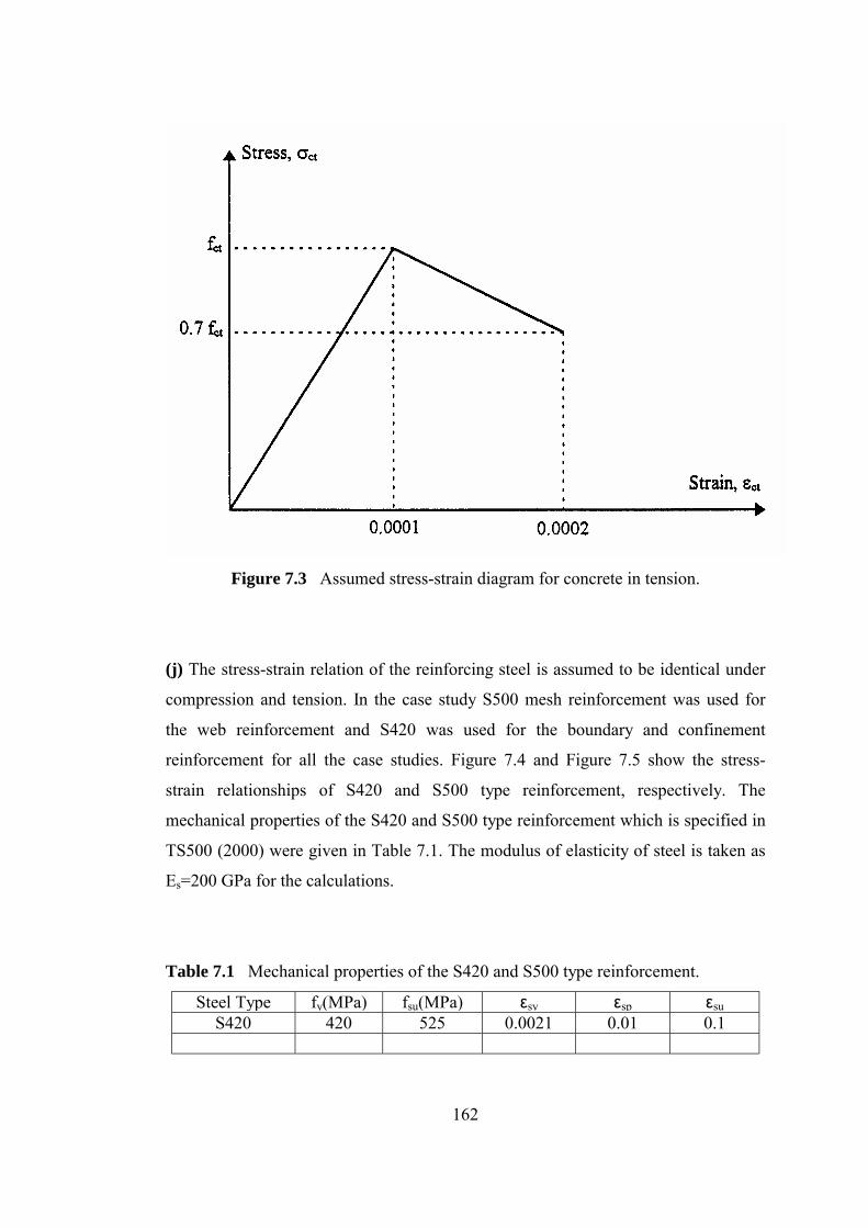
162
Figure 7.3 Assumed stress-strain diagram for concrete in tension.
(j) The stress-strain relation of the reinforcing steel is assumed to be identical under
compression and tension. In the case study S500 mesh reinforcement was used for
the web reinforcement and S420 was used for the boundary and confinement
reinforcement for all the case studies. Figure 7.4 and Figure 7.5 show the stress-
strain relationships of S420 and S500 type reinforcement, respectively. The
mechanical properties of the S420 and S500 type reinforcement which is specified in
TS500 (2000) were given in Table 7.1. The modulus of elasticity of steel is taken as
Es=200 GPa for the calculations.
Table 7.1 Mechanical properties of the S420 and S500 type reinforcement.
Steel Type fy(MPa) fsu(MPa) εsy εsp εsu S420 420 525 0.0021 0.01 0.1

163
Figure 7.4 Assumed tri-linear stress-strain curve for S420 type reinforcement.
Figure 7.5 Assumed bi-linear stress-strain curve for S500 type reinforcement.
164
7.3 BASIC ALGORITHM
The cross section is idealized as a series of unconfined and confined concrete
rectangular layers and steel layers that are each parallel to the neutral axis. It is
assumed that the strain in each layer is uniform and equal to the actual strain at the
center of the layer. The stress will also be taken as uniform over the layer and found
from the assumed stress-strain relations. The force in each layer is found by
multiplying the stress in the layer by the area of the layer. The moment contribution
is found by multiplying the layer force by the distance between the middle of the
layer and the plastic centroid of the cross-section. The stress resultants are
determined by evaluating the forces in each layer of concrete and each layer of
reinforcement. Obviously the idealization becomes more accurate as the layers
become narrower, so layers of 1 mm thickness are used in this study. The theoretical
moment curvature relation for a given axial load level can be determined by
increasing the concrete strain in the extreme compression fiber. Iteration was started
with a low extreme concrete fiber strain. This is a rather small strain value for
concrete in compression. The analysis procedure involves the following steps:
1) Assign an initial value for the compressive strain at the extreme concrete fiber. An
initial top strain value of -0.00001 is assigned in this study. However, in the analysis
of some sections the force equilibrium cannot be found for small values of top strain,
like -0.00001. In order to prevent this situation, the program finds the smallest top
strain value at which the force equilibrium is satisfied and takes this value as the
initial top strain and continues the process.
2) Assume a neutral axis depth. The depth of neutral axis is iterated starting from an
initial value of 4 times the depth of the section until the force equilibrium is reached.
3) Calculate strains at the middle of each fiber.
4) Use stress-strain models for confined and unconfined concrete to determine the
stress values at each fiber.

165
5) Determine the longitudinal steel strains from similar triangles of the strain
diagram.
6) With the steel strain at each level, steel stresses are determined from the stress-
strain diagram of steel. Forces in steel in each level are obtained by multiplying these
stresses by the respective steel areas.
7) On the compression side, with the concrete strains at each fiber, concrete stresses
are determined by entering the stress-strain curves of confined or unconfined
concrete. Forces in confined and unconfined concrete fibers are obtained by
multiplying these stresses by respective areas.
8) On the tension side, tensile stresses at each fiber are obtained by entering the
stress strain curve of concrete in tension. Forces in concrete on the tension side are
obtained by multiplying these stresses by the filament area.
9) Compute the sum of the internal forces and compare this with the external axial
force. If the difference is less than or equal to 0.1%, results are acceptable.
Otherwise, the position of the neutral axis is changed (go to step 2) until equilibrium
is satisfied.
10) Calculate moment and curvature values. After the neutral axis depth
corresponding to an extreme fiber strain is found, the total moment is calculated by
summing up the fiber moments and the moments of longitudinal reinforcements
about the plastic centroid of the section. Fiber moments are calculated by multiplying
the fiber force by the distance from the middle of fiber to the geometric center of the
section. Curvature is obtained by dividing the top fiber strain by the neutral axis
depth. Top strain, bottom stain and the neutral axis depth are written corresponding
to the moment-curvature values on the ‘output sheet’.
11) Set the new concrete strain and go back to the step 2. Top strain value is assigned
increasing the previous top strain value by 0.00001. When the force equilibrium at a
top strain cannot be found, the program ends the process.

166
7.4 CURVATURE DUCTILITY
The most common and desirable sources of inelastic structural deformations
are rotations in potential plastic hinges. Therefore, it is useful to relate section
rotations per unit length (i.e., curvature) to causative bending moments. Curvature
ductility ratios are calculated by dividing ultimate curvatures by yield curvatures and
expressed as:
yu / φφ=µφ (7.8)
The moment-curvature relation of a wall or wall system analyzed can be
idealized by an approximated elastoplastic or bilinear moment-curvature relation in
order to find the curvature ductility in a simpler way of solution. First yield is
defined as the moment and curvature corresponding to syy E/f=ε , where the
bottom tensile reinforcement starts to yield. For shear wall sections where there are
many steel layers the yield curvature yφ has to be defined. While assuming the
bilinear relation, one must determine the yield curvature and corresponding yield
moment to be used for this relation. In order to find this yield curvature, an
approximation is made as described below.
• A tangent line is drawn to the first yield point on the moment-curvature
diagram.
• The second line is drawn assuming the approximate increasing linear path
after the yield point on the moment-curvature diagram.
• The yield curvature and the corresponding moment is found as the point
where these two lines intersect.
The approximation procedure and the bilinear curve obtained are shown in
Figure 7.6.

167
Figure 7.6 Determination process for bilinear moment-curvature diagram.
It is obvious that the yield curvature obtained from this assumption is a higher
value from the first yield point, however especially in structural walls, this may be a
good approximation as the walls are reinforced all along the wall length and so there
is more than one layer of steel in the tension zone.
7.5 CASE AND VERIFICATION STUDIES
Four cases were investigated in this study. The analyses were based on a
shear wall 4.6 m long and 200 mm wide, with fck = 20 MPa. The axial load
compressive stress (N/Ag) was 2.17 MPa corresponding to an axial load ratio of
N/fckAg = 0.108. In all cases boundary elements are provided at a distance of
lu = 0.206×lw = 950 mm from each end of the wall. The spacing of the longitudinal
boundary reinforcement is 150 mm. Web reinforcement ratio is taken as 0.25% for
shear walls in all cases for this study. To provide 0.25% web reinforcement ratio in
the vertical and horizontal directions, 7 mm diameter two-layer mesh reinforcement
(S500) was used in the web regions for shear walls. The spacing of longitudinal and
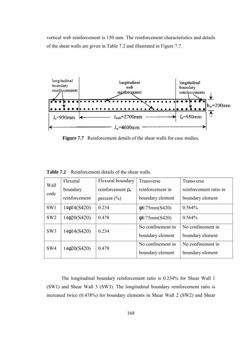
168
vertical web reinforcement is 150 mm. The reinforcement characteristics and details
of the shear walls are given in Table 7.2 and illustrated in Figure 7.7.
Figure 7.7 Reinforcement details of the shear walls for case studies.
Table 7.2 Reinforcement details of the shear walls.
Wall
code
Flexural
boundary
reinforcement
Flexural boundary
reinforcement ρb
percent (%)
Transverse
reinforcement in
boundary element
Transverse
reinforcement ratio in
boundary element
SW1 14φ14(S420) 0.234 φ8/75mm(S420) 0.564%
SW2 14φ20(S420) 0.478 φ8/75mm(S420) 0.564%
SW3 14φ14(S420) 0.234 No confinement in
boundary element
No confinement in
boundary element
SW4 14φ20(S420) 0.478 No confinement in
boundary element
No confinement in
boundary element
The longitudinal boundary reinforcement ratio is 0.234% for Shear Wall 1
(SW1) and Shear Wall 3 (SW3). The longitudinal boundary reinforcement ratio is
increased twice (0.478%) for boundary elements in Shear Wall 2 (SW2) and Shear

169
Wall 4 (SW4) to study the effect of the longitudinal boundary reinforcement ratio of
shear walls. 8 mm diameter transverse reinforcement with 75 mm spacing is used to
confine the boundary elements in SW1 and SW2. The reinforcement detail for
confined boundary regions of SW1 and SW2 is shown in Figure 7.8. The transverse
reinforcement ratio is 0.564% for boundary elements in these two walls. Boundary
elements in Shear Wall 3 and Shear Wall 4 are not confined so as to be able to
observe the confinement effect in shear walls.
Figure 7.8 Reinforcement detail for confined boundary regions of SW1 and SW2.
7.6 SHEAR WALL 1 (SW1)
For this first case a detailed explanation was presented about the moment
curvature diagram and relationship to be able to show the behavior of the wall. The
calculated response of SW1 is summarized in Table 7.3 and illustrated in
Figure 7.9.
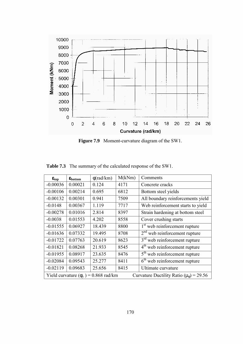
170
Figure 7.9 Moment-curvature diagram of the SW1.
Table 7.3 The summary of the calculated response of the SW1.
εεεεtop εεεεbottom φ(rad/km) M(kNm) Comments -0.00036 0.00021 0.124 4171 Concrete cracks -0.00106 0.00214 0.695 6812 Bottom steel yields -0.00132 0.00301 0.941 7509 All boundary reinforcements yield -0.0148 0.00367 1.119 7717 Web reinforcement starts to yield -0.00278 0.01016 2.814 8397 Strain hardening at bottom steel -0.0038 0.01553 4.202 8558 Cover crushing starts -0.01555 0.06927 18.439 8800 1st web reinforcement rupture -0.01636 0.07332 19.495 8708 2nd web reinforcement rupture -0.01722 0.07763 20.619 8623 3rd web reinforcement rupture -0.01821 0.08268 21.933 8545 4th web reinforcement rupture -0.01955 0.08917 23.635 8476 5th web reinforcement rupture -0.02084 0.09543 25.277 8411 6th web reinforcement rupture -0.02119 0.09683 25.656 8415 Ultimate curvature Yield curvature (φy ) = 0.868 rad/km Curvature Ductility Ratio (µφ) = 29.56
171
For a large moment the concrete remains uncracked. Cracking marks the
points where the moment-curvature relationship begins to change its slope. The
initial change in slope immediately after cracking is rather small. When the applied
moment is greater than 7509 kN all the boundary reinforcement in the tension side
yields. After that the web reinforcements start to yield, strain hardening starts at the
outermost longitudinal boundary reinforcement and the moment curvature diagram
get rounded in nature. We can see from the moment curvature diagrams that there is
a small change for moment corresponding to the extreme compression fiber strain
-0.0038 (φ=4.202 rad/km M=8558 kNm). When the extreme compression fiber strain
reaches -0.0038 the unconfined cover concrete start to crush. After a small decrease
in moment, it starts to increase again slowly according to the ductility of the section.
After the spalling of the top cover concrete is completed, cover crushing continues at
the edges of confined boundary regions. At a moment of 8800 kNm the strain in the
lowest layer of the web reinforcement (S500) is predicted to be 0.0501. This value of
strain will cause rupture of this reinforcement. Five more web reinforcements
reached their ultimate strain (εsu=0.05) and ruptured consecutively as can be
observed from the moment-curvature diagram. At a curvature value of 25.656 rad/km
the strain in the outermost layer of the longitudinal boundary reinforcement (S420) is
0.097. Rupture of this reinforcement defines the capacity of the member. At this
stage cover concrete with a length of 678 mm (82% of the neutral axis depth) from
the compression edge of the wall spalled. Confined concrete in the confined
boundary region was not crushed. Failure of the Shear Wall 1 occurs by rupturing of
the reinforcement rather than by crushing of the concrete.
7.7 SHEAR WALL 2 (SW2)
The moment curvature curve of the SW1 and SW2 is plotted on the same
graph to be able to compare the effect of longitudinal boundary reinforcement ratio
in shear walls that have confined boundary elements at each end of the wall. The

172
calculated response of SW2 is summarized in Table 7.4 and illustrated in
Figure 7.10.
Figure 7.10 Moment curvature diagram of SW1 and SW2.
Table 7.4 The summary of the calculated response of the SW2.
εεεεtop εεεεbottom φ(rad/km) M(kNm) Comments -0.00035 0.00021 0.122 4487 Concrete cracks -0.00119 0.00214 0.725 9595 Bottom steel yields -0.0015 0.00304 0.988 10796 All boundary reinforcements yield -0.0167 0.00373 1.175 11043 Web reinforcement yields -0.00301 0.0102 2.873 11827 Strain hardening at bottom steel -0.0038 0.01421 3.915 11975 Cover crushing starts -0.01679 0.06961 18.783 12546 1st web reinforcement rupture -0.01775 0.07388 19.92 12479 2nd web reinforcement rupture -0.01874 0.07825 21.085 12417 3rd web reinforcement rupture -0.02003 0.08357 22.522 12366 4th web reinforcement rupture -0.02119 0.08766 23.662 12394 Ultimate curvature Yield curvature (φy ) = 0.905 rad/km Curvature ductility ratio (µφ) = 26.15
173
The overall behavior of SW1 and SW2 is identical. Failure occurs similar to
SW1 by rupturing of the lowest four layers of web reinforcement and the outermost
level of longitudinal boundary reinforcement. At this stage the cover concrete with a
length of 735mm (82% of the neutral axis depth) from the compression edge of the
wall spalled. Confined concrete in the confined boundary region was not crushed.
As a result of two times, increase in the longitudinal boundary reinforcement
ratio, a 40% increase in moment capacity is observed. However the ductility of the
system reduces slightly. There is a 4.3% increase in yield curvature. The ultimate
curvature and curvature ductility ratios decrease 7.8% and 11.5%, respectively.
7.8 SHEAR WALL 3 (SW3) and SHEAR WALL 4 (SW4)
SW3 and SW4 are analyzed with both Waller2002 and Response2000. Two
moment curvature curves obtained from these programs were plotted on the same
graph to be able to examine the differences. It is seen from Figure 7.11 that the
moment curvature curves obtained by these programs are close to each other. The
small difference at ultimate curvature is due to the models used for unconfined
concrete. The Hognestad model and parabolic models are used in Waller 2002 and
Response2000, respectively.
The overall behavior of SW3 and SW4 is almost the same. The behavior of
SW3 and SW4 is explained and calculated responses are summarized in Table 7.5
and Table 7.6, respectively, according to the output of Waller2002. For SW1 and
SW3 at the bottom concrete strain of 0.00021 concrete cracks and the slope of
moment curvature curves is changed. Before the unconfined cover concrete crushes
(εcontop=-0.0038) all the longitudinal boundary reinforcement and the outermost mesh
reinforcement yield. Even strain hardening starts at the bottom layer of the
longitudinal boundary reinforcement in both cases. Both shear walls show brittle
failure and their failure occurs by crushing of the concrete, reinforcement rupture
does not occur in either case.
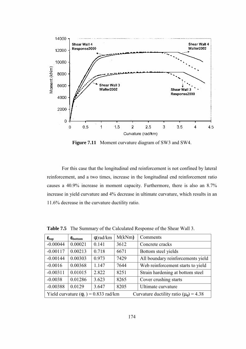
174
Figure 7.11 Moment curvature diagram of SW3 and SW4.
For this case that the longitudinal end reinforcement is not confined by lateral
reinforcement, and a two times, increase in the longitudinal end reinforcement ratio
causes a 40.9% increase in moment capacity. Furthermore, there is also an 8.7%
increase in yield curvature and 4% decrease in ultimate curvature, which results in an
11.6% decrease in the curvature ductility ratio.
Table 7.5 The Summary of the Calculated Response of the Shear Wall 3.
εεεεtop εεεεbottom φ(rad/km M(kNm) Comments -0.00044 0.00021 0.141 3612 Concrete cracks -0.00117 0.00213 0.718 6671 Bottom steel yields -0.00144 0.00303 0.973 7429 All boundary reinforcements yield -0.0016 0.00368 1.147 7644 Web reinforcement starts to yield -0.00311 0.01015 2.822 8251 Strain hardening at bottom steel -0.0038 0.01286 3.623 8265 Cover crushing starts -0.00388 0.0129 3.647 8205 Ultimate curvature Yield curvature (φy ) = 0.833 rad/km Curvature ductility ratio (µφ) = 4.38
175
Table 7.6 The Summary of the calculated response of the Shear Wall 4.
εεεεtop εεεεbottom φ(rad/km M(kNm) Comments -0.00043 0.00021 0.14 3956 Concrete cracks -0.00128 0.00215 0.745 9474 Bottom steel yields -0.00159 0.00305 1.01 10717 All boundary reinforcements yield -0.00176 0.00373 1.192 10967 Web reinforcement starts to yield -0.00338 0.01041 2.999 11635 Strain hardening at bottom steel -0.0038 0.01205 3.445 11653 Cover crushing starts -0.0396 0.01215 3.503 11524 Ultimate curvature Yield curvature (φy ) = 0.906 rad/km Curvature ductility ratio (µφ) = 3.87
7.9 MOMENT-CURVATURE RESPONSE OF THE PANEL FORM TEST
SPECIMENS
In this part, moment-curvature response of the panel form test specimens SP1
and SP2 are obtained both by the Waller2002 and Response2000. The results
obtained by the computer programs Waller2002 and Response2000 are compared
and discussed. Characteristic compression strength and tension strength of the
concrete are taken as 35 MPa and 2.07 MPa, respectively. The shape of the stress-
strain diagram of the concrete under compression and tension are as given in Figure
7.1 and 7.3. εy = 0.00275, εu = 0.025, fsy = 550 MPa and fsu=600 MPa are the yield
strain, ultimate strain, yield strength, ultimate strength values of the reinforcing steel,
respectively. Rupturing of the longitudinal reinforcement occurred for both SP1 and
SP2. While evaluating the computer output results, it is realized that for both SP1
and SP2 rupturing of the longitudinal reinforcement occurred. A detailed
investigation and nomenclatures of the moment-curvature response of the panel form
tests are given in Chapter 8.
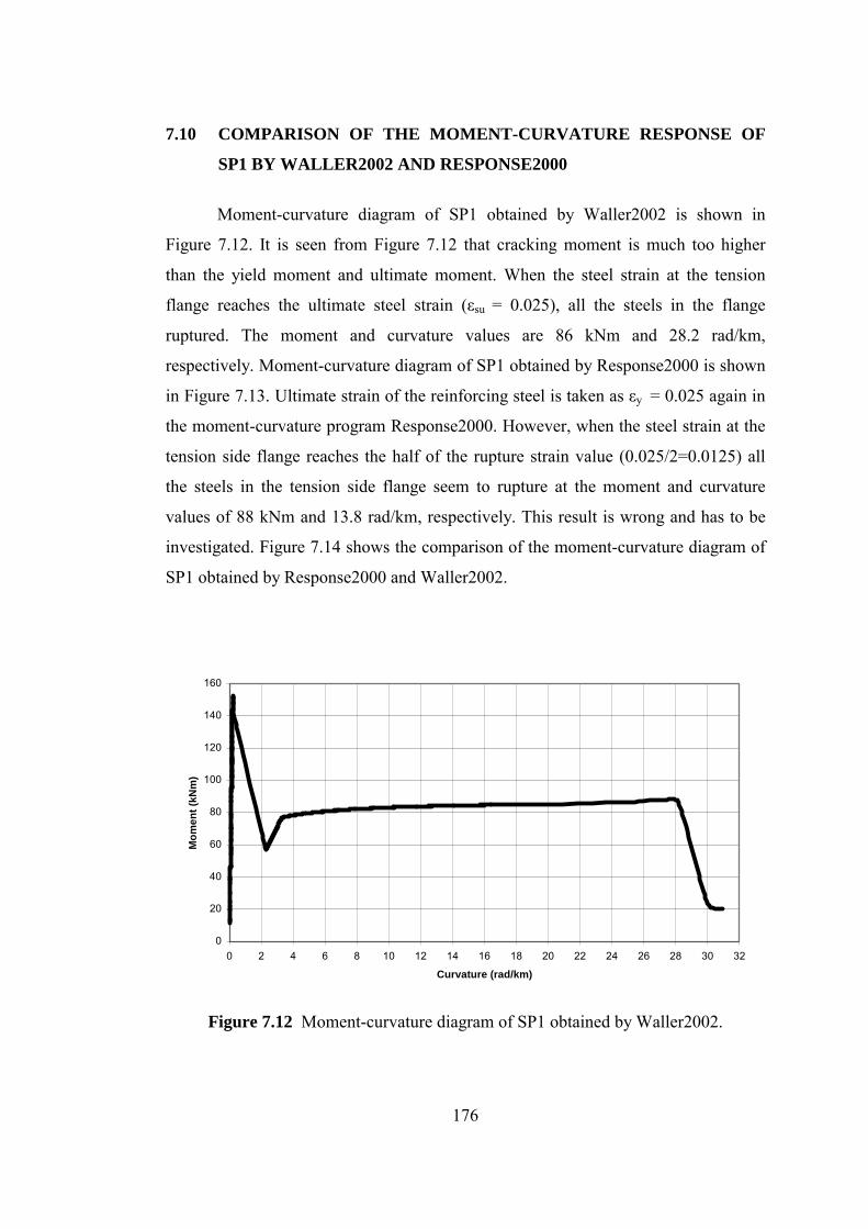
176
7.10 COMPARISON OF THE MOMENT-CURVATURE RESPONSE OF
SP1 BY WALLER2002 AND RESPONSE2000
Moment-curvature diagram of SP1 obtained by Waller2002 is shown in
Figure 7.12. It is seen from Figure 7.12 that cracking moment is much too higher
than the yield moment and ultimate moment. When the steel strain at the tension
flange reaches the ultimate steel strain (εsu = 0.025), all the steels in the flange
ruptured. The moment and curvature values are 86 kNm and 28.2 rad/km,
respectively. Moment-curvature diagram of SP1 obtained by Response2000 is shown
in Figure 7.13. Ultimate strain of the reinforcing steel is taken as εy = 0.025 again in
the moment-curvature program Response2000. However, when the steel strain at the
tension side flange reaches the half of the rupture strain value (0.025/2=0.0125) all
the steels in the tension side flange seem to rupture at the moment and curvature
values of 88 kNm and 13.8 rad/km, respectively. This result is wrong and has to be
investigated. Figure 7.14 shows the comparison of the moment-curvature diagram of
SP1 obtained by Response2000 and Waller2002.
0
20
40
60
80
100
120
140
160
0 2 4 6 8 10 12 14 16 18 20 22 24 26 28 30 32
Curvature (rad/km)
Mom
ent (
kNm
)
Figure 7.12 Moment-curvature diagram of SP1 obtained by Waller2002.
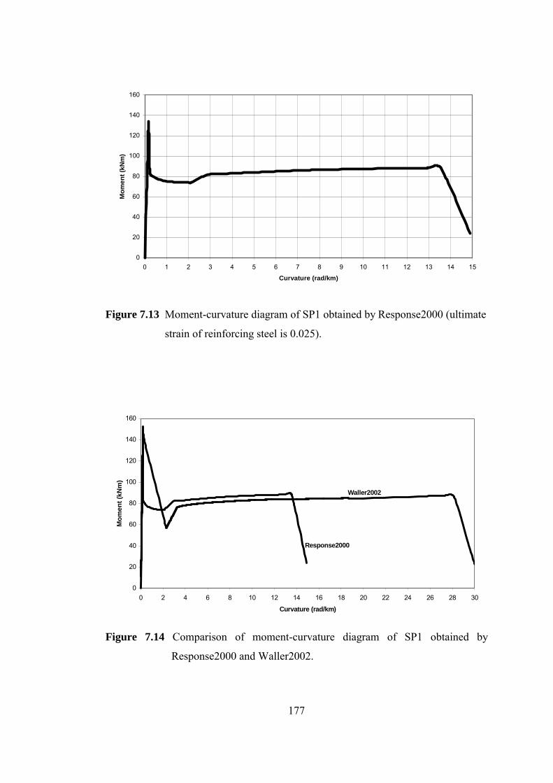
177
0
20
40
60
80
100
120
140
160
0 1 2 3 4 5 6 7 8 9 10 11 12 13 14 15
Curvature (rad/km)
Mom
ent (
kNm
)
Figure 7.13 Moment-curvature diagram of SP1 obtained by Response2000 (ultimate
strain of reinforcing steel is 0.025).
0
20
40
60
80
100
120
140
160
0 2 4 6 8 10 12 14 16 18 20 22 24 26 28 30
Curvature (rad/km)
Mom
ent (
kNm
)
Waller2002
Response2000
Figure 7.14 Comparison of moment-curvature diagram of SP1 obtained by
Response2000 and Waller2002.
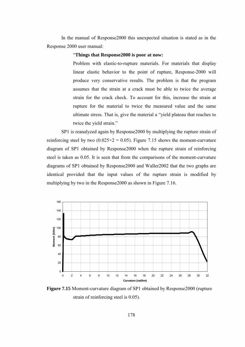
178
In the manual of Response2000 this unexpected situation is stated as in the
Response 2000 user manual:
“Things that Response2000 is poor at now:
Problem with elastic-to-rupture materials. For materials that display
linear elastic behavior to the point of rupture, Response-2000 will
produce very conservative results. The problem is that the program
assumes that the strain at a crack must be able to twice the average
strain for the crack check. To account for this, increase the strain at
rupture for the material to twice the measured value and the same
ultimate stress. That is, give the material a “yield plateau that reaches to
twice the yield strain.”
SP1 is reanalyzed again by Response2000 by multiplying the rupture strain of
reinforcing steel by two (0.025×2 = 0.05). Figure 7.15 shows the moment-curvature
diagram of SP1 obtained by Response2000 when the rupture strain of reinforcing
steel is taken as 0.05. It is seen that from the comparisons of the moment-curvature
diagrams of SP1 obtained by Response2000 and Waller2002 that the two graphs are
identical provided that the input values of the rupture strain is modified by
multiplying by two in the Response2000 as shown in Figure 7.16.
0
20
40
60
80
100
120
140
160
0 2 4 6 8 10 12 14 16 18 20 22 24 26 28 30 32
Curvature (rad/km)
Mom
ent (
kNm
)
Figure 7.15 Moment-curvature diagram of SP1 obtained by Response2000 (rupture
strain of reinforcing steel is 0.05).
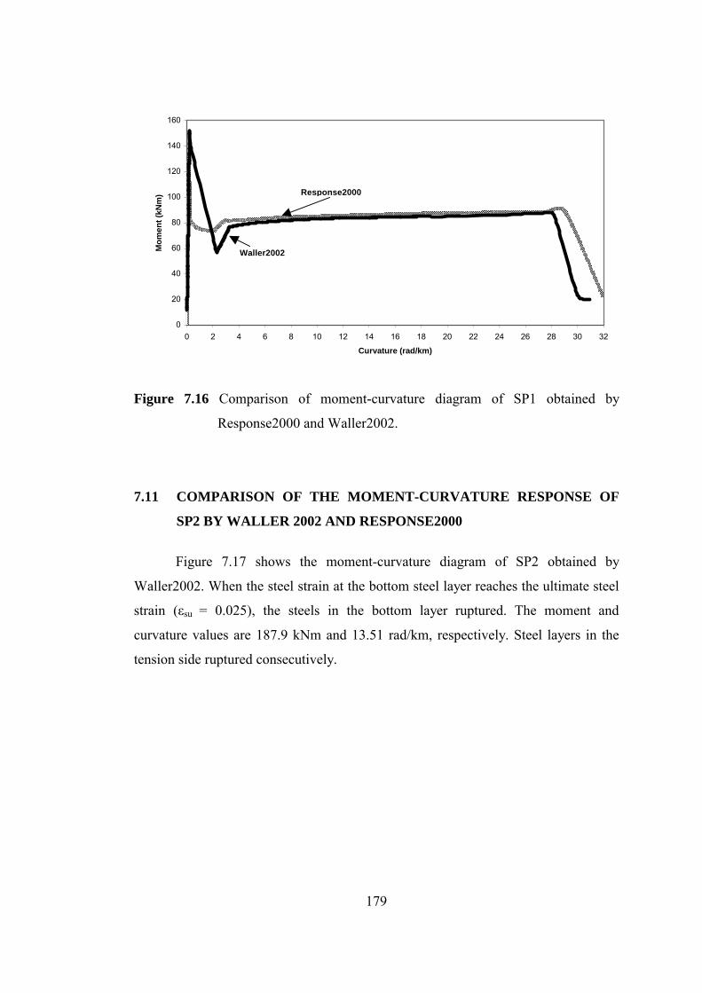
179
��������������������
��������
�������������������������������������������������������������������������������������������������������������������������������������������������������������������������������������������������������������������������������������������������������������������������������������������������������������������������������������������������������������������������������������������������������������������������������������������������������������������������������������������������������������������������������
������������������������������������������������������������������������������������
���������������������������������������������������������������������������������������������������������������������������������������������������������������������������������
������������
��������������������������������������������������������
������������������������������������������������
��������������������������������������������
��������������������������������������������
��������������������������������������������
������������������������������
������������������������������
��������������������������������������������������������������������������������������������������������������������������������������������������������������������������������������������������������������������������������������������������������������������������������������������������������������������������������������������������������������������������������������������������������������������������������������
����������������������������������
������������������������������������
��������������������������
���������������������������������
0
20
40
60
80
100
120
140
160
0 2 4 6 8 10 12 14 16 18 20 22 24 26 28 30 32
Curvature (rad/km)
Mom
ent (
kNm
) Response2000
Waller2002
Figure 7.16 Comparison of moment-curvature diagram of SP1 obtained by
Response2000 and Waller2002.
7.11 COMPARISON OF THE MOMENT-CURVATURE RESPONSE OF
SP2 BY WALLER 2002 AND RESPONSE2000
Figure 7.17 shows the moment-curvature diagram of SP2 obtained by
Waller2002. When the steel strain at the bottom steel layer reaches the ultimate steel
strain (εsu = 0.025), the steels in the bottom layer ruptured. The moment and
curvature values are 187.9 kNm and 13.51 rad/km, respectively. Steel layers in the
tension side ruptured consecutively.

180
0
20
40
60
80
100
120
140
160
180
200
0 1 2 3 4 5 6 7 8 9 10 11 12 13 14 15 16 17 18 19 20
Curvature (rad/km)
Mom
ent (
kNm
)
Figure 7.17 Moment-curvature diagram of SP2 obtained by Waller2002.
Figure 7.18 shows the moment-curvature diagram of SP2 obtained by
Response2000. Ultimate strain of the reinforcing is steel taken as εy = 0.025 again in
the moment-curvature program Response2000. Figure 7.19 shows the comparison of
moment-curvature diagram of SP2 obtained by Response2000 and Waller2002 when
the ultimate strain of the reinforcing steel is 0.025. The same problem explained in
the previous part occurred again in Response2000. Ultimate curvature of SP2
obtained by Response2000 is again occurring at the half of the rupture strain value
(0.025/2=0.0125). Ultimate strain of the reinforcing steel is taken as εy = 0.025,
again in the moment-curvature program Response2000. However, when the steel
strain at the bottom steel layer in the tension side reaches the half of the rupture
strain value (0.025/2=0.0125) steels in this layer seem to rupture at the moment and
curvature values of 176.37 kNm and 7.03 rad/km, respectively.

181
0
20
40
60
80
100
120
140
160
180
200
0 1 2 3 4 5 6 7 8 9 10 11 12
Curvature (rad/km)
Mom
ent (
kNm
)
Figure 7.18 Moment-curvature diagram of SP2 obtained by Response2000 (ultimate
strain of reinforcing steel is 0.025).
������������������������
��������
�������������������������������������������������������������������������������������������������������������������������������������������������������������������������������������������������������������������������������������������������������������������������������������������������������������������������������������������������������������������������������������������������������������������������������������
����������������������������������������������������������������������������������������������������������������������������������������������������������
�����������������������������������������������������������
�������������������������������������������
�����������������������������������������������������������������������������������������������������������
������������
��������������������
���������������������������������������������������������������������������������������������������������������������������
�������������������������������������������������������
��������������������������������
�����������������������������
����������������������������������
��������������������������������������������������������������
������������������������������������������������������
�������������������������������������
0
20
40
60
80
100
120
140
160
180
200
0 1 2 3 4 5 6 7 8 9 10 11 12 13 14 15 16 17 18 19 20
Curvature (rad/km)
Mom
ent (
kNm
)
Waller2002
Response2000
Figure 7.19 Comparison of moment-curvature diagram of SP2 obtained by
Response2000 and Waller2002 (ultimate strain of the reinforcing
steel is 0.025).
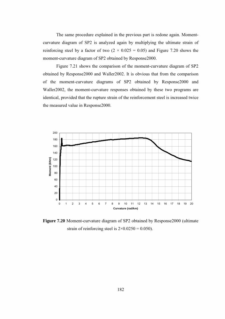
182
The same procedure explained in the previous part is redone again. Moment-
curvature diagram of SP2 is analyzed again by multiplying the ultimate strain of
reinforcing steel by a factor of two (2 × 0.025 = 0.05) and Figure 7.20 shows the
moment-curvature diagram of SP2 obtained by Response2000.
Figure 7.21 shows the comparison of the moment-curvature diagram of SP2
obtained by Response2000 and Waller2002. It is obvious that from the comparison
of the moment-curvature diagrams of SP2 obtained by Response2000 and
Waller2002, the moment-curvature responses obtained by these two programs are
identical, provided that the rupture strain of the reinforcement steel is increased twice
the measured value in Response2000.
0
20
40
60
80
100
120
140
160
180
200
0 1 2 3 4 5 6 7 8 9 10 11 12 13 14 15 16 17 18 19 20
Curvature (rad/km)
Mom
ent (
kNm
)
Figure 7.20 Moment-curvature diagram of SP2 obtained by Response2000 (ultimate
strain of reinforcing steel is 2×0.0250 = 0.050).
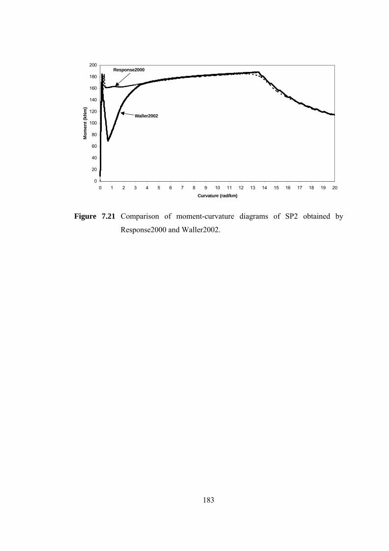
183
0
20
40
60
80
100
120
140
160
180
200
0 1 2 3 4 5 6 7 8 9 10 11 12 13 14 15 16 17 18 19 20
Curvature (rad/km)
Mom
ent (
kNm
)
Waller2002
Response2000
Figure 7.21 Comparison of moment-curvature diagrams of SP2 obtained by
Response2000 and Waller2002.

184
CHAPTER 8
DISCUSSION AND EVALUATION OF THE TEST RESULTS
8.1 GENERAL
In this chapter, the experimental results of the static tests are evaluated and
discussed by considering strength, stiffness, response, energy dissipation and drift
characteristics of the test specimens.
Figure 8.1 General view of the panel form test specimens SP1 and SP2.

185
Figure 8.1 shows the general view of the panel form test specimens SP1 and
SP2. The test specimen which was tested in the short dimension is called
SPECIMEN1 (SP1) and the one which was tested in the long dimension is called
SPECIMEN2 (SP2). SP1 is located at the right hand side and SP2 is located at the
left hand side in Figure 8.1. The weigths of the panel form test specimens SP1 and
SP2 are 24.66 kN and this value is used in all the calculations. The axial load
compressive stress (N/Ag) was 0.128 MPa corresponding to an axial load ratio of
N/fckAg = 0.00367.
8.2 PROPERTIES OF THE TEST SPECIMENS
Concrete compressive strength of the panel form test specimens is 35 MPa. In
the new Turkish Code (TS-500, 2000), the direct tensile strength is expressed as a
function of the square root of the compression strength:
MPa07.2f35.0f ckctk == (8.1)
In the Turkish Code (TS-500, 2000), it is also specified that the tensile
strength obtained from flexure tests are 2 times the direct tensile strength:
MPa14.4f7.0f ckctf == (8.2)
Concrete is not a linearly elastic material. Therefore, it is difficult to justify
any definition for the modulus of elasticity of concrete. Since the slope of the σ-ε
curve of concrete is not constant, one has to describe modulus of elasticity, Ec, before
defining such a term. In general the modulus of elasticity defined for concrete is the
instantaneous Ec, which is not influenced by the time effect. The instantaneous
modulus of elasticity of concrete can be defined in three different ways as stated
below (Ersoy and Özcebe, 2001):
a) Initial modulus (Tangent to the curve at the origin)
b) Secant modulus (slope of the secant at a given stress; usually 0.5 fc)
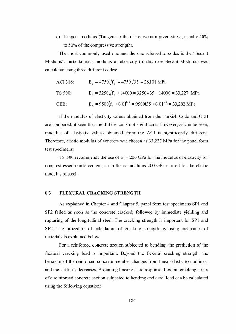
186
c) Tangent modulus (Tangent to the σ-ε curve at a given stress, usually 40%
to 50% of the compressive strength).
The most commonly used one and the one referred to codes is the “Secant
Modulus”. Instantaneous modulus of elasticity (in this case Secant Modulus) was
calculated using three different codes: ACI 318: MPa101,28354750f4750E c ===c
TS 500: MPa227,331400035325014000f3250E c =+=+=c
CEB: ( ) ( ) MPa282,330.83595000.8f9500E 3/13/1c =+=+=c
If the modulus of elasticity values obtained from the Turkish Code and CEB
are compared, it seen that the difference is not significant. However, as can be seen,
modulus of elasticity values obtained from the ACI is significantly different.
Therefore, elastic modulus of concrete was chosen as 33,227 MPa for the panel form
test specimens.
TS-500 recommends the use of Es = 200 GPa for the modulus of elasticity for
nonprestressed reinforcement, so in the calculations 200 GPa is used for the elastic
modulus of steel.
8.3 FLEXURAL CRACKING STRENGTH
As explained in Chapter 4 and Chapter 5, panel form test specimens SP1 and
SP2 failed as soon as the concrete cracked; followed by immediate yielding and
rupturing of the longitudinal steel. The cracking strength is important for SP1 and
SP2. The procedure of calculation of cracking strength by using mechanics of
materials is explained below.
For a reinforced concrete section subjected to bending, the prediction of the
flexural cracking load is important. Beyond the flexural cracking strength, the
behavior of the reinforced concrete member changes from linear-elastic to nonlinear
and the stiffness decreases. Assuming linear elastic response, flexural cracking stress
of a reinforced concrete section subjected to bending and axial load can be calculated
using the following equation:
187
IyM
AN ⋅±=σ (8.3)
The cracking moment Mcr, can be calculated by substituting M = Mcr and
σ = fctf into Equation (8.3):
−=
yI
ANfM ctfcr (8.4)
where
fctf : flexural tensile strength of concrete, ckctf ff 7.0= (MPa)
I : moment of inertia of the concrete section
y : distance between the centroid and extreme tension fiber
N : total axial load applied on the section
A : gross cross-sectional area
The lateral load corresponding to the flexural cracking (Vfcr) could be
calculated by assuming the panel form test specimens as a cantilever.
HMV cr
fcr = (8.5)
where
H : Distance between the lateral load and the cracking surface of the test
specimens.
8.4 PROPERTIES OF SP1
Figure 8.2 shows the reinforcement pattern and loading direction of the shear
walls of the panel form test specimen SP1.

188
Figure 8.2 Reinforcement pattern and loading direction of SP1. (All dimensions are
in mm).
The modular ratio, the total area of the wall reinforcement in the longitudinal
direction, the cross-sectional wall area, the longitudinal reinforcement ratio, the
transformed area, the gross and transformed moment of inertia and the flexural
rigidity of SP1 are summarized in the following.
The modular ratio for SP1 is calculated as shown in the following
0.6MPa227,33MPa000,200
EE
n ===
c
s
Total area of the wall reinforcement in the longitudinal direction for SP1 is
2mm305A =steel
Cross-sectional wall area for SP1 is
Aconcrete = 192,000 mm2

189
Longitudinal reinforcement ratio for SP1 is
00159.0mm000,192
mm305AA
2
2
=
=
=ρ
c
ss
The transformed area of SP1 is calculated by considering the individual steel
layers and found as
Atrans = 193,524 mm2
Gross and transformed moment of inertia along the short dimension of SP1 is
calculated as
ISP1gross = 2.995 × 10⁻² m4
ISP1trans = 3.019 × 10⁻² m4
Flexural rigidity for the transformed case of SP1 is
Ec × ISP1trans = = 1,003,121 kNm2
It is seen that the gross and transformed moment of inertia of SP1 are very
close to each other because longitudinal reinforcement ratio is low. For simplicity
gross moment of inertia can be used in practice but in this study transformed moment
of inertia will be used.
From Equation (8.4), moment corresponding to the flexural cracking was
calculated and found as
Mcr = 275.3 kNm
From Equation (8.5), shear force corresponding to the flexural cracking was
calculated as
kN1.103 m67.2
kNm3.275H
MV cr
fcr ===
During the static tests of SP1, the horizontal flexural crack, which caused the
failure, was observed at 35 kN load level. These differences were due to probability
of defects (like voids, large aggregates, local cracks etc.) and the low reinforcement
ratio.
190
8.5 PRESENTATION OF THE STATIC TEST RESULTS FOR SP1
The observed behavior of SP1 is presented in this section. Lateral load-
displacement curves for the 1st and 2nd static tests for SP1 were given separately in
Chapter 4. In this chapter the 1st and 2nd static tests are combined, considered and
presented as a single test.
Lateral load displacement curves of the 1st, 2nd, 3rd and 4th stories are given in
Figures 8.3, 8.4, 8.5 and 8.6, respectively. The maximum applied lateral load was
40 kN for SP1. Maximum lateral-displacements are 2 mm, 4 mm, and 6 mm, for the
1st, 2nd and 3rd story levels, respectively. The maximum displacement and yield
displacement are 3.5 mm and 8.6 mm, respectively, at the fourth story level as seen
in Figure 8.6. The displacement ductility factor for SP1 is µ∆ = 2.46.
µ∆ (SP1) = 2.46 < µ∆ (required) = 4~5
The displacement ductility of SP1 is lower than the required displacement
ductility. It is obvious from the above equation that SP1 shows brittle failure.
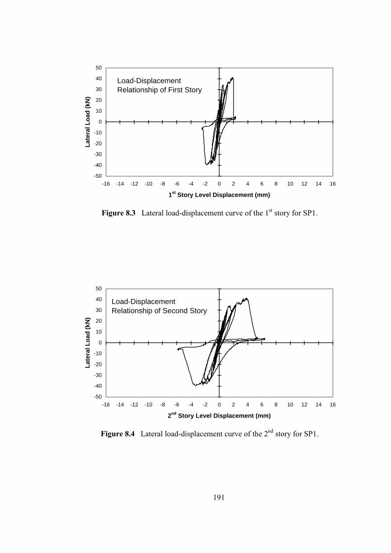
191
-50
-40
-30
-20
-10
0
10
20
30
40
50
-16 -14 -12 -10 -8 -6 -4 -2 0 2 4 6 8 10 12 14 16
1st Story Level Displacement (mm)
Late
ral L
oad
(kN
)Load-DisplacementRelationship of First Story
Figure 8.3 Lateral load-displacement curve of the 1st story for SP1.
-50
-40
-30
-20
-10
0
10
20
30
40
50
-16 -14 -12 -10 -8 -6 -4 -2 0 2 4 6 8 10 12 14 16
2nd Story Level Displacement (mm)
Late
ral L
oad
(kN
)
Load-DisplacementRelationship of Second Story
Figure 8.4 Lateral load-displacement curve of the 2nd story for SP1.

192
-50
-40
-30
-20
-10
0
10
20
30
40
50
-16 -14 -12 -10 -8 -6 -4 -2 0 2 4 6 8 10 12 14 16
3th Story Level Displacement (mm)
Late
ral L
oad
(kN
)Load-DisplacementRelationship of Third Story
Figure 8.5 Lateral load-displacement curve of the 3rd story for SP1.
-50
-40
-30
-20
-10
0
10
20
30
40
50
-16 -14 -12 -10 -8 -6 -4 -2 0 2 4 6 8 10 12 14 16
4th Story Level Displacement (mm)
Late
ral L
oad
(kN
)
Load-DisplacementRelationship of Fourth Story
Figure 8.6 Lateral load-displacement curve of the 4th story for SP1.

193
The observed behavior of SP1 in the static tests can be summarized as
follows:
• SP1 exhibits horizontal tension cracking at the flanges.
• As the concrete cracks, longitudinal reinforcements yield at the crack
location.
• SP1 fails, as soon as the concrete cracks followed by yielding and then
rupturing of the longitudinal steel.
• Crushing of the concrete is not observed.
• The cracking moment and yield moment are very close to each other.
• Unloaded tension force in the flanges after cracking cannot be carried by the
minimum amounts of reinforcement.
The observations of the laboratory tests demonstrate that SP1 is susceptible to
a brittle material failure. This brittle mode of flexural failure is directly linked to the
low-reinforcement ratio of SP1.
8.6 STRENGTH AND CURVATURE DUCTILITY OF SP1
The ultimate flexural capacities of SP1 and SP2 were calculated using the
computer program, Response-2000. The analytical interaction diagram for SP1 is
shown in Figure 8.7.
It is seen from Figure 8.7 that the axial tension load capacity of SP1 is
183 kN and axial compression load capacity of SP1 is 5880 kN. Constant axial load
on SP1, which is -24.66 kN, is shown as a bold horizontal line. At the balanced case,
the axial load and moment are 1133 kN and 2980 kNm, respectively. It is seen from
the analytical interaction curve that the axial load level on SP1 is very low.
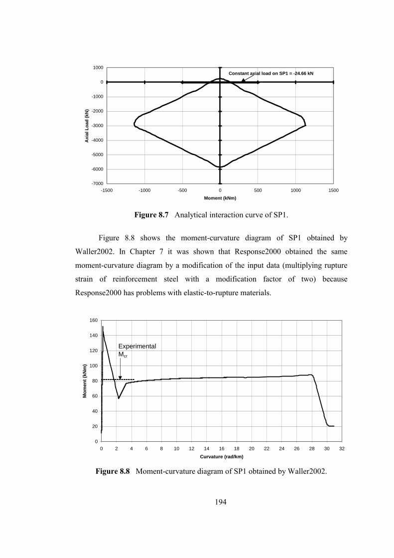
194
-7000
-6000
-5000
-4000
-3000
-2000
-1000
0
1000
-1500 -1000 -500 0 500 1000 1500Moment (kNm)
Axi
al L
oad
(kN
)
Constant axial load on SP1 = -24.66 kN
Figure 8.7 Analytical interaction curve of SP1.
Figure 8.8 shows the moment-curvature diagram of SP1 obtained by
Waller2002. In Chapter 7 it was shown that Response2000 obtained the same
moment-curvature diagram by a modification of the input data (multiplying rupture
strain of reinforcement steel with a modification factor of two) because
Response2000 has problems with elastic-to-rupture materials.
Figure 8.8 Moment-curvature diagram of SP1 obtained by Waller2002.
0
20
40
60
80
100
120
140
160
0 2 4 6 8 10 12 14 16 18 20 22 24 26 28 30 32Curvature (rad/km)
Mom
ent (
kNm
)
ExperimentalMcr

195
For a large moment range, up to 152.3 kNm, SP1 remains uncracked. When
the extreme tension concrete fiber strain reaches 0.0001, the moment reaches 152.3
kNm. This moment value is the maximum moment value where the curvature is
0.205 rad/km at this stage. Cracking marks the point where the moment-curvature
relationship falls down sharply. It is seen that from the moment curvature diagram
cracking moment is 1.8 times greater than the ultimate moment. When the extreme
tension concrete fiber strain reaches 0.0002, the moment reaches 140.2 kNm and the
curvature is 0.298 rad/km. After tension cracking, the moment value falls down from
152.3 kNm to 57.07 kNm value. When the moment value is 57.07 kNm, the
curvature and bottom steel strain values are 2.3 rad/km and 0.00194, respectively. As
soon as the concrete cracks all the longitudinal flange reinforcement in the tension
flange yields. Then the moment values start to increase again and when the moment
and curvature values reach 76.57 kNm and 3.275 rad/km, respectively, the bottom
steel yields, 2nd and 3th layer reinforcements yield consecutively. Nominal yield is
found as 3.57 rad/km and the corresponding moment values are found as 77.34 kNm,
as explained in Chapter 7. All the web reinforcements yield consecutively. Moment-
curvature diagram is horizontal at that level. It is seen from Figure 8.8 and Table 8.1
that when the steel strain value at the flange of SP1 reaches the rupture strain of the
reinforcement (0.025), all the steels at the tension side flange rupture. Ultimate
moment and ultimate curvature are 86 kNm and 28.2 rad/km, respectively.
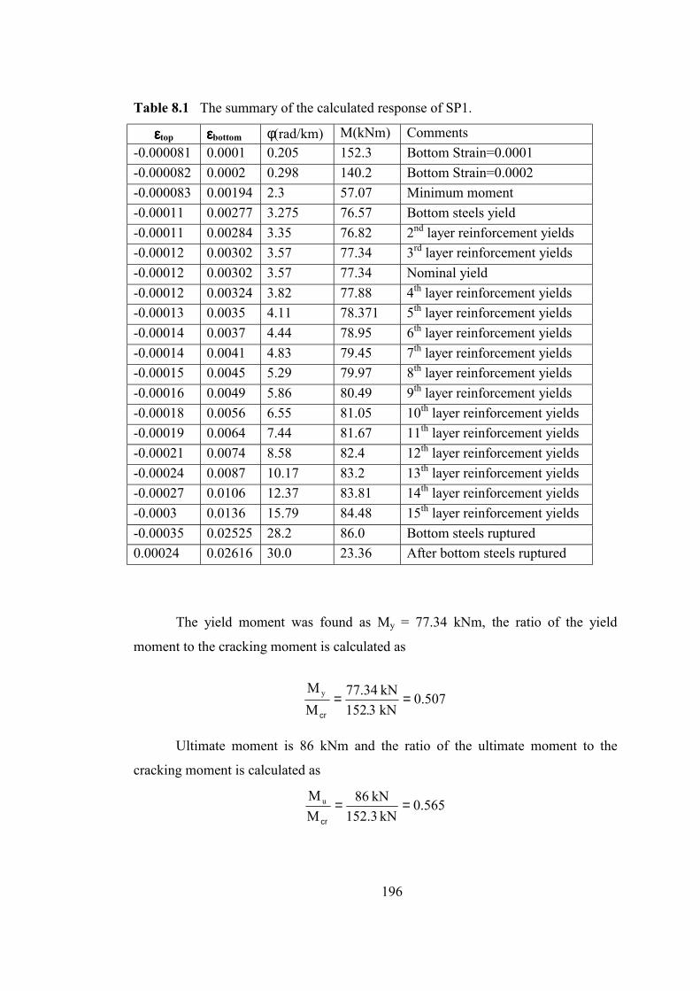
196
Table 8.1 The summary of the calculated response of SP1.
εεεεtop εεεεbottom φ(rad/km) M(kNm) Comments -0.000081 0.0001 0.205 152.3 Bottom Strain=0.0001 -0.000082 0.0002 0.298 140.2 Bottom Strain=0.0002 -0.000083 0.00194 2.3 57.07 Minimum moment -0.00011 0.00277 3.275 76.57 Bottom steels yield -0.00011 0.00284 3.35 76.82 2nd layer reinforcement yields -0.00012 0.00302 3.57 77.34 3rd layer reinforcement yields -0.00012 0.00302 3.57 77.34 Nominal yield -0.00012 0.00324 3.82 77.88 4th layer reinforcement yields -0.00013 0.0035 4.11 78.371 5th layer reinforcement yields -0.00014 0.0037 4.44 78.95 6th layer reinforcement yields -0.00014 0.0041 4.83 79.45 7th layer reinforcement yields -0.00015 0.0045 5.29 79.97 8th layer reinforcement yields -0.00016 0.0049 5.86 80.49 9th layer reinforcement yields -0.00018 0.0056 6.55 81.05 10th layer reinforcement yields -0.00019 0.0064 7.44 81.67 11th layer reinforcement yields -0.00021 0.0074 8.58 82.4 12th layer reinforcement yields -0.00024 0.0087 10.17 83.2 13th layer reinforcement yields -0.00027 0.0106 12.37 83.81 14th layer reinforcement yields -0.0003 0.0136 15.79 84.48 15th layer reinforcement yields -0.00035 0.02525 28.2 86.0 Bottom steels ruptured 0.00024 0.02616 30.0 23.36 After bottom steels ruptured
The yield moment was found as My = 77.34 kNm, the ratio of the yield
moment to the cracking moment is calculated as
507.0 kN3.152kN34.77
MM y ==
cr
Ultimate moment is 86 kNm and the ratio of the ultimate moment to the
cracking moment is calculated as
565.0kN3.152
kN86MM u ==
cr
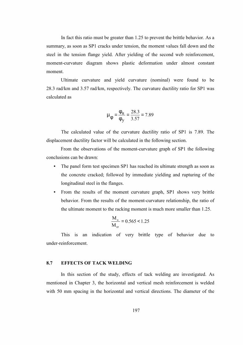
197
In fact this ratio must be greater than 1.25 to prevent the brittle behavior. As a
summary, as soon as SP1 cracks under tension, the moment values fall down and the
steel in the tension flange yield. After yielding of the second web reinforcement,
moment-curvature diagram shows plastic deformation under almost constant
moment.
Ultimate curvature and yield curvature (nominal) were found to be
28.3 rad/km and 3.57 rad/km, respectively. The curvature ductility ratio for SP1 was
calculated as
89.757.3
3.28
yu ===φ φ
φµ
The calculated value of the curvature ductility ratio of SP1 is 7.89. The
displacement ductility factor will be calculated in the following section.
From the observations of the moment-curvature graph of SP1 the following
conclusions can be drawn:
• The panel form test specimen SP1 has reached its ultimate strength as soon as
the concrete cracked; followed by immediate yielding and rupturing of the
longitudinal steel in the flanges.
• From the results of the moment curvature graph, SP1 shows very brittle
behavior. From the results of the moment-curvature relationship, the ratio of
the ultimate moment to the racking moment is much more smaller than 1.25.
25.1565.0MM u <=
cr
This is an indication of very brittle type of behavior due to
under-reinforcement.
8.7 EFFECTS OF TACK WELDING
In this section of the study, effects of tack welding are investigated. As
mentioned in Chapter 3, the horizontal and vertical mesh reinforcement is welded
with 50 mm spacing in the horizontal and vertical directions. The diameter of the
198
horizontal and vertical mesh reinforcement is 2 mm. To determine stress-strain
relationship of reinforcing steel, randomly taken test coupons were tested under
tension. The longitudinal and horizontal mesh reinforcements were plain bars. Yield
and ultimate strengths of reinforcing steel are fsy = 550 MPa and fsu = 600 MPa,
respectively.
In shear walls, steel bars with 2 mm diameter and in the slabs, steel bars with
2.5 mm diameter are used as reinforcing bars. To obtain the characteristic values of
mesh reinforcement, randomly taken six specimens were tested under uniaxial
tension test before the welding process. From the visual observations, it can be
concluded that after tack welding there is no decrement in the area of the mesh
reinforcement. The lengths of the reinforcements are 2 m before tack welding
process. Test specimen lengths of the reinforcement bars are 100 mm. Table 8.2
shows the mechanical properties of the reinforcing bars before the tack welding
process.
Table 8.2 Mechanical properties of the reinforcing bars before tack welding.
Steel No fsy(MPa) fsu (MPa) εsy εsu
φφφφ2 550 650 0.0027 0.03
φφφφ2.5 550 650 0.0027 0.03
After obtaining the mechanical properties of the reinforcement, tack welding
process is applied to the reinforcements. The spacing of the mesh reinforcement is
50 mm in horizontal and vertical directions. Table 8.2 shows the mechanical
properties of the reinforcing bars after tack welding process.

199
Table 8.3 Mechanical properties of the reinforcing bars after tack welding .
Steel No fsy(MPa) fsu (MPa) εsy εsu
φφφφ2 540 600 0.0027 0.025
φφφφ2.5 540 600 0.0027 0.025
From the comparisons of Table 8.2 and Table 8.3 it is seen that the ultimate
strength of the reinforcing steel decreases 7.7 % and the ultimate strain of the
reinforcing steel decreases 16 % due to tack welding process. Yield strength of the
reinforcing steel decreases 1.82 % due to tack welding process.
After the tension test of the mesh reinforcement, the following observation is
obtained. Rupturing of the mesh reinforcement does not occur exactly at the tack
welding point, but occurs 5~10 mm away from the tack welding point.
In the following section ductility and strength reduction due to tack welding
of the reinforcing steel are investigated by changing the yield strength and yield
strain, ultimate strength and ultimate strain values. To improve the brittle behavior,
boundary reinforcement is provided at the boundary regions of the test specimen.
The boundary reinforcement is provided according to the Turkish Seismic Code
(AY-1997).
8.8 EFFECTS OF TACK WELDING ON SP1
8.8.1 Ductility Reduction
In this section ultimate strain of the reinforcing steel is changed and the
obtained moment-curvature behavior is discussed. The moment-curvature diagram of
SP1 is drawn by assuming for ultimate steel strain єsu = 0.01, єsu = 0.015,
єsu = 0.020, єsu = 0.025, єsu = 0.030, єsu = 0.035, єsu = 0.040 єsu = 0.045 and єsu =
0.050. Figure 8.9 shows the effects of ultimate strain of reinforcing steel on the
moment-curvature behavior of SP1. It is seen from Figure 8.9 that the general
behavior is the same when the rupture strain of reinforcing steel is changed from 0.01
to 0.05. Observed cracking moment in the static tests of SP1 is 81 kNm.
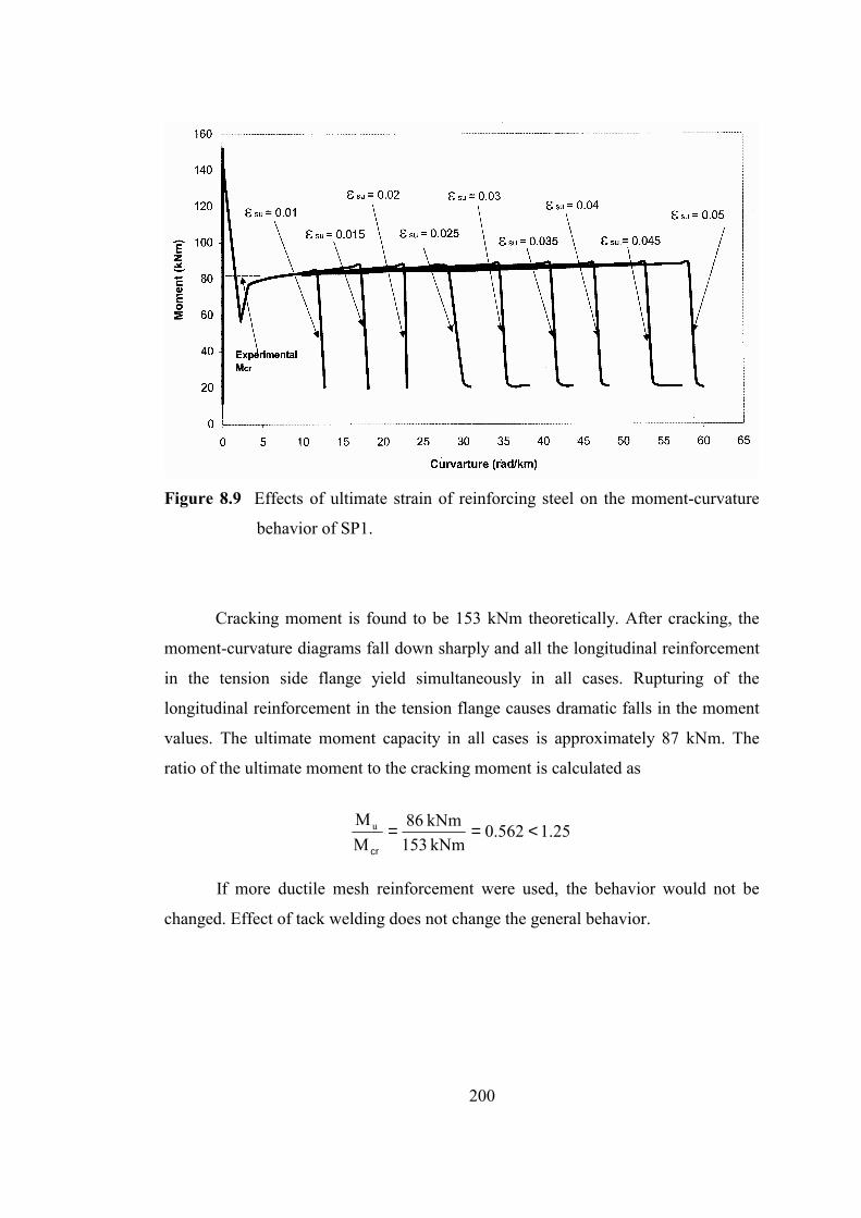
200
Figure 8.9 Effects of ultimate strain of reinforcing steel on the moment-curvature
behavior of SP1.
Cracking moment is found to be 153 kNm theoretically. After cracking, the
moment-curvature diagrams fall down sharply and all the longitudinal reinforcement
in the tension side flange yield simultaneously in all cases. Rupturing of the
longitudinal reinforcement in the tension flange causes dramatic falls in the moment
values. The ultimate moment capacity in all cases is approximately 87 kNm. The
ratio of the ultimate moment to the cracking moment is calculated as
25.1562.0kNm153kNm86
MM u <==
cr
If more ductile mesh reinforcement were used, the behavior would not be
changed. Effect of tack welding does not change the general behavior.
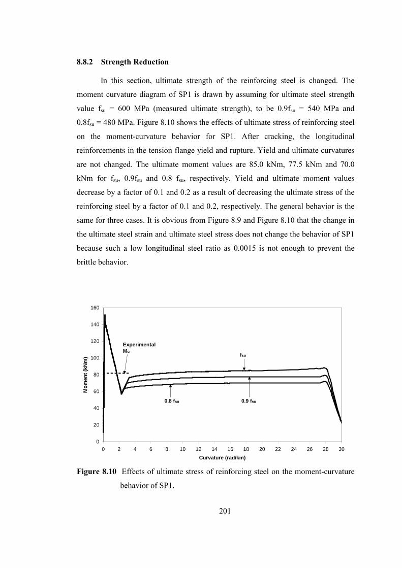
201
8.8.2 Strength Reduction
In this section, ultimate strength of the reinforcing steel is changed. The
moment curvature diagram of SP1 is drawn by assuming for ultimate steel strength
value fsu = 600 MPa (measured ultimate strength), to be 0.9fsu = 540 MPa and
0.8fsu = 480 MPa. Figure 8.10 shows the effects of ultimate stress of reinforcing steel
on the moment-curvature behavior for SP1. After cracking, the longitudinal
reinforcements in the tension flange yield and rupture. Yield and ultimate curvatures
are not changed. The ultimate moment values are 85.0 kNm, 77.5 kNm and 70.0
kNm for fsu, 0.9fsu and 0.8 fsu, respectively. Yield and ultimate moment values
decrease by a factor of 0.1 and 0.2 as a result of decreasing the ultimate stress of the
reinforcing steel by a factor of 0.1 and 0.2, respectively. The general behavior is the
same for three cases. It is obvious from Figure 8.9 and Figure 8.10 that the change in
the ultimate steel strain and ultimate steel stress does not change the behavior of SP1
because such a low longitudinal steel ratio as 0.0015 is not enough to prevent the
brittle behavior.
0
20
40
60
80
100
120
140
160
0 2 4 6 8 10 12 14 16 18 20 22 24 26 28 30Curvature (rad/km)
Mom
ent (
kNm
)
0.9 fsu0.8 fsu
fsu
ExperimentalMcr
Figure 8.10 Effects of ultimate stress of reinforcing steel on the moment-curvature
behavior of SP1.

202
8.9 BOUNDARY REINFORCEMENT EFFECTS ON SP1
The Turkish Earthquake Code AY-1997, imposes certain regulations and
restrictions on structural walls. The plastic hinge region is typically located at the
base of a cantilever wall where significant flexural deformations occur. The primary
longitudinal reinforcement used to develop the resisting moment is concentrated at
both ends of the wall. For slender structural walls ( )2/H ww >l , which are
categorized as the high ductility class, the critical wall length is defined as
(hcr = max [lw, Hw/6]). In the critical wall length, confined boundary elements have to
be provided at a distance of wu 2.0 ll ×≥ from each end of the wall. In this region the
longitudinal reinforcement ratio must be at least 0.2% of the gross section. For non-
ductile shear walls or outside the critical wall length, boundary elements have to be
provided at a distance of wu 1.0 ll ×≥ from each end of the wall. In this region the
longitudinal reinforcement ratio must be at least 0.1% of the gross section. Figures
8.11 and 8.12 show the reinforcement pattern and loading direction of SP1 with
boundary reinforcement ratios of 0.001 bw lw and 0.002 bw lw, respectively. Boundary
reinforcement that is used in this study is assumed to be S420 type reinforcement,
which has ultimate strain and strength values of єsu = 0.1 and fsu = 0.525 MPa,
respectively.
Three cases are compared in Figure 8.13. The boundary regions are provided
at a distance of wu 1.0 ll ×≥ and wu 2.0 ll ×≥ , boundary reinforcement ratio is 0.1%
and 0.2%, respectively for the gross wall area in the direction of loading.
Placing the boundary reinforcement only in the web direction does not change
the behavior. The same brittle behavior is observed again. Longitudinal flange
reinforcements yield as soon as the section cracks. After the rupturing of the mesh
reinforcement in the flange, moment values fall down sharply again as in the
previous case.

203
SP1
Loading direction
F
lb > 0.1 lw = 100 mm
ρb = 0.001 bw lw
Figure 8.11 Reinforcement pattern and loading direction of SP1 with boundary
reinforcement ratio of 0.001 bw lw.
SP1
Loading direction
F
lu > 0.2 lw = 200 mm
ρu = 0.002 bw lw
Figure 8.12 Reinforcement pattern and loading direction of SP1 with boundary
reinforcement ratio of 0.002 bw lw.
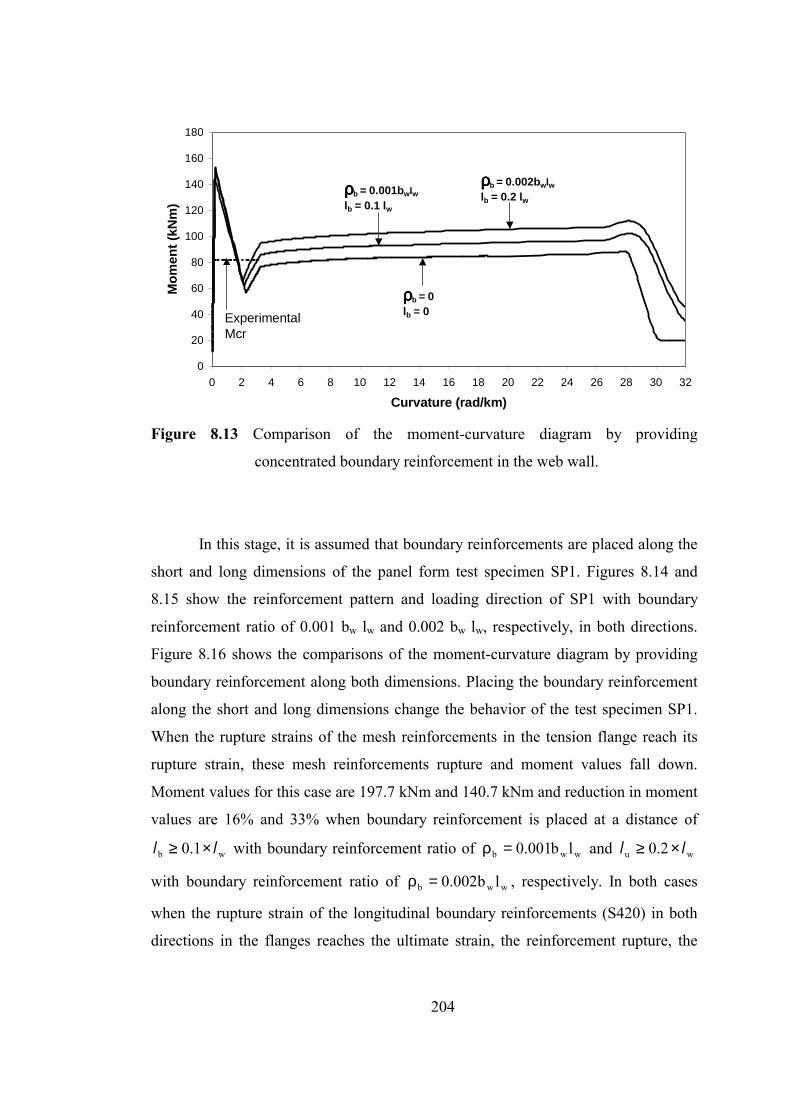
204
Figure 8.13 Comparison of the moment-curvature diagram by providing
concentrated boundary reinforcement in the web wall.
In this stage, it is assumed that boundary reinforcements are placed along the
short and long dimensions of the panel form test specimen SP1. Figures 8.14 and
8.15 show the reinforcement pattern and loading direction of SP1 with boundary
reinforcement ratio of 0.001 bw lw and 0.002 bw lw, respectively, in both directions.
Figure 8.16 shows the comparisons of the moment-curvature diagram by providing
boundary reinforcement along both dimensions. Placing the boundary reinforcement
along the short and long dimensions change the behavior of the test specimen SP1.
When the rupture strains of the mesh reinforcements in the tension flange reach its
rupture strain, these mesh reinforcements rupture and moment values fall down.
Moment values for this case are 197.7 kNm and 140.7 kNm and reduction in moment
values are 16% and 33% when boundary reinforcement is placed at a distance of
wb 1.0 ll ×≥ with boundary reinforcement ratio of wwb lb001.0=ρ and wu 2.0 ll ×≥
with boundary reinforcement ratio of wwb lb002.0=ρ , respectively. In both cases
when the rupture strain of the longitudinal boundary reinforcements (S420) in both
directions in the flanges reaches the ultimate strain, the reinforcement rupture, the
0
20
40
60
80
100
120
140
160
180
0 2 4 6 8 10 12 14 16 18 20 22 24 26 28 30 32
Curvature (rad/km)
Mom
ent (
kNm
)ρρρρb = 0.001bwlwlb = 0.1 lw
ρρρρb = 0.002bwlwlb = 0.2 lw
ρρρρb = 0lb = 0Experimental
Mcr

205
ultimate curvature and ultimate moment values are obtained. Mu / Mcr =
140.7 kNm / 155 kNm = 0.9 and Mu / Mcr = 197.7 kNm / 160.5 kNm = 1.23 when
boundary reinforcement is placed at a distance of wu 1.0 ll ×≥ and wu 2.0 ll ×≥ ,
respectively. It is obvious form Figure 8.16 when the boundary reinforcement is
placed at a distance of wu 2.0 ll ×≥ with boundary reinforcement ratio
wwb lb002.0=ρ the behavior is not brittle as in the previous case. Ultimate moment
Mu is nearly 1.25 times Mcr.
SP1
Loading direction
F
lu > 0.1 lw in both direction ρu = 0.001 bw lw
Figure 8.14 Reinforcement pattern and loading direction of SP1 with boundary
reinforcement ratio of 0.001 bw lw in both directions.

206
SP1
Loading direction
F
lb > 0.2 lw in both direction ρb = 0.002 bw lw
Figure 8.15 Reinforcement pattern and loading direction of SP1 with boundary
reinforcement ratio of 0.002 bw lw in both direstions.
Figure 8.16 Comparisons of the moment-curvature diagram by providing boundary
reinforcement along both dimensions.
0
20
40
60
80
100
120
140
160
180
200
220
0 10 20 30 40 50 60 70 80 90 100 110 120 130Curvature (rad/km)
Mom
ent (
kNm
)
ρρρρb = 0.001bwlwlb = 0.1 lw in both directions
ρρρρb = 0.002bwlwlb = 0.2 lw in both directions
ρρρρb = 0.002bwlw lb = 0.2 lwρρρρb = 0.001bwlw lb = 0.1 lwρρρρb = 0 lb = 0

207
8.10 PROPERTIES OF SP2
Figure 8.17 shows the reinforcement pattern and loading direction of the
shear walls of the panel form test specimen SP2.
Figure 8.17 Reinforcement pattern and loading direction of SP2. (All dimensions
are in mm).
The modular ratio, the total area of the wall reinforcement in the longitudinal
direction, the cross-sectional wall area, the longitudinal reinforcement ratio, the
transformed area, the gross and transformed moment of inertia and the flexural
rigidity of SP2 is summarized in the following.
The modular ratio for SP2 is calculated as
0.6MPa227,33MPa000,200
EE
n ===
c
s
Total area of the wall reinforcement in the longitudinal direction for SP2 is
2mm305A =steel
208
Cross-sectional wall area for SP2 is
Aconcrete = 192,000 mm2
Longitudinal reinforcement ratio for SP2 is
00159.0mm000,192
mm305AA
2
2
=
=
=ρ
c
ss
The transformed area of SP2 is calculated by considering the individual steel
layers and found as
Atrans = 193,524 mm2
Gross and transformed moment of inertia along the short dimension of SP2 is
calculated as
ISP2gross = 5.334 × 10⁻² m4
ISP2trans = 5.355 × 10⁻² m4
Flexural rigidity of SP2 is calculated as
Ec × ISP2trans = 1,779,217 kNm2
It is seen that the gross and transformed moment of inertia of SP2 is very
close to each other because longitudinal reinforcement ratio is low as in the case of
SP1.
From Equation (8.4), moment corresponding to the first flexural cracking was
calculated
Mcr = 214.88 kNm
From Equation (8.4), shear corresponding to the first flexural cracking was
calculated
kN48.80m67.2kNm88.214
HM
V crfcr
===
During the static test of panel form test specimen SP2, the crack, which
caused the failure of SP2, was observed at about 70 kN load level.
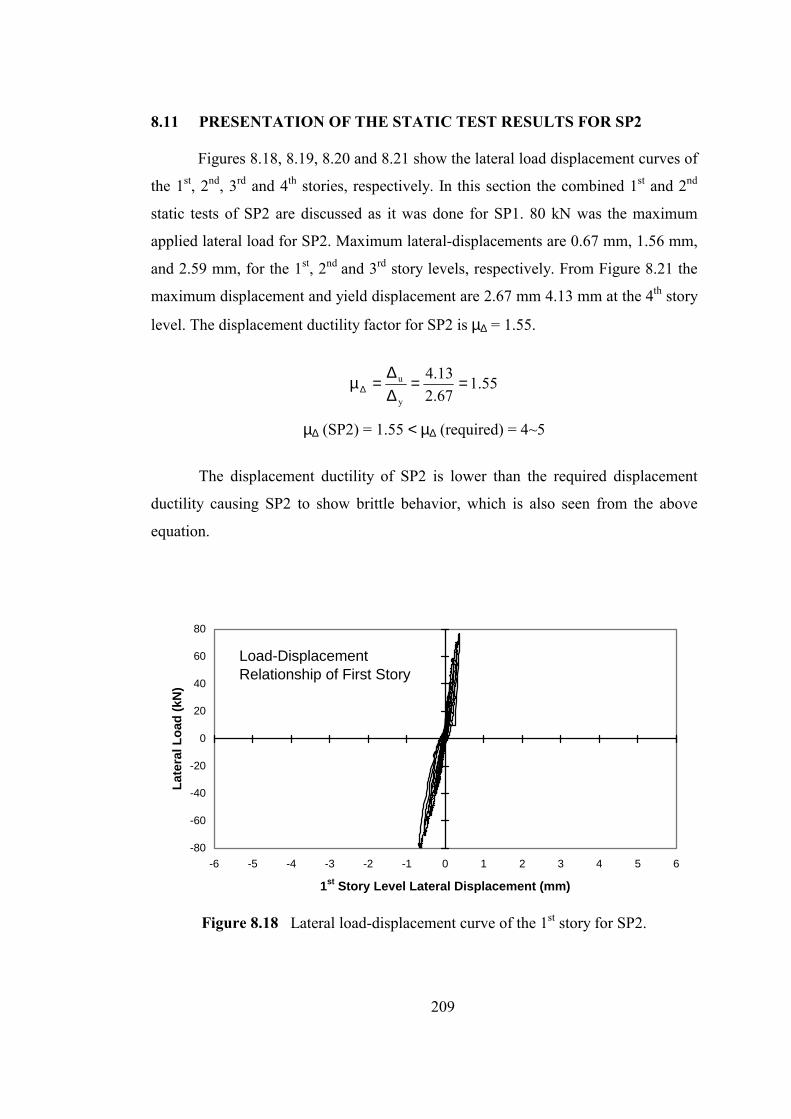
209
8.11 PRESENTATION OF THE STATIC TEST RESULTS FOR SP2
Figures 8.18, 8.19, 8.20 and 8.21 show the lateral load displacement curves of
the 1st, 2nd, 3rd and 4th stories, respectively. In this section the combined 1st and 2nd
static tests of SP2 are discussed as it was done for SP1. 80 kN was the maximum
applied lateral load for SP2. Maximum lateral-displacements are 0.67 mm, 1.56 mm,
and 2.59 mm, for the 1st, 2nd and 3rd story levels, respectively. From Figure 8.21 the
maximum displacement and yield displacement are 2.67 mm 4.13 mm at the 4th story
level. The displacement ductility factor for SP2 is µ∆ = 1.55.
55.167.213.4
y
u ==∆∆
=µ∆
µ∆ (SP2) = 1.55 < µ∆ (required) = 4~5
The displacement ductility of SP2 is lower than the required displacement
ductility causing SP2 to show brittle behavior, which is also seen from the above
equation.
-80
-60
-40
-20
0
20
40
60
80
-6 -5 -4 -3 -2 -1 0 1 2 3 4 5 6
1st Story Level Lateral Displacement (mm)
Late
ral L
oad
(kN
)
Load-DisplacementRelationship of First Story
Figure 8.18 Lateral load-displacement curve of the 1st story for SP2.

210
-80
-60
-40
-20
0
20
40
60
80
-6 -5 -4 -3 -2 -1 0 1 2 3 4 5 6
2nd Story Level Displacement (mm)
Late
ral L
oad
(kN
m)
Load-DisplacementRelationship of Second Story
Figure 8.19 Lateral load-displacement curve of the 2nd story for SP2.
-80
-60
-40
-20
0
20
40
60
80
-6 -5 -4 -3 -2 -1 0 1 2 3 4 5 6
3rd Story Level Displacement (mm)
Late
ral L
oad
(kN
)
Load-DisplacementRelationship of Third Story
Figure 8.20 Lateral load-displacement curve of the 3rd story for SP2.
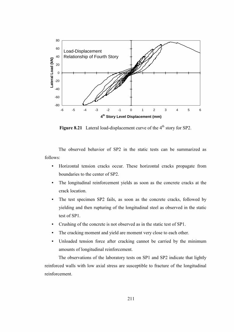
211
-80
-60
-40
-20
0
20
40
60
80
-6 -5 -4 -3 -2 -1 0 1 2 3 4 5 6
4th Story Level Displacement (mm)
Late
ral L
oad
(kN
)Load-DisplacementRelationship of Fourth Story
Figure 8.21 Lateral load-displacement curve of the 4th story for SP2.
The observed behavior of SP2 in the static tests can be summarized as
follows:
• Horizontal tension cracks occur. These horizontal cracks propagate from
boundaries to the center of SP2.
• The longitudinal reinforcement yields as soon as the concrete cracks at the
crack location.
• The test specimen SP2 fails, as soon as the concrete cracks, followed by
yielding and then rupturing of the longitudinal steel as observed in the static
test of SP1.
• Crushing of the concrete is not observed as in the static test of SP1.
• The cracking moment and yield are moment very close to each other.
• Unloaded tension force after cracking cannot be carried by the minimum
amounts of longitudinal reinforcement.
The observations of the laboratory tests on SP1 and SP2 indicate that lightly
reinforced walls with low axial stress are susceptible to fracture of the longitudinal
reinforcement.

212
8.12 STRENGTH AND CURVATURE DUCTILITY OF SP2
Figure 8.22 shows the analytical interaction diagram of SP2. Axial tension
load capacity of SP2 is 183 kN and axial compression load capacity of SP2 is 5880
kN. Axial tension and compression load capacity of SP1 and SP2 are the same
because they have the same cross-section but loading direction is perpendicular to
each other. Bold horizontal line just below the zero axial load axes shows the
constant axial load (-24.66 kN) on SP2. At the balanced case, axial load and moment
is 1133 kN and 2980 kNm, respectively. It is seen from the analytical interaction
curve that the axial load level on SP2 is very low.
-7000
-6000
-5000
-4000
-3000
-2000
-1000
0
1000
-1500 -1000 -500 0 500 1000 1500Curvature (rad/km)
Mom
ent (
kNm
)
Constant axial load on SP2 = -24.66 kN
Figure 8.22 Analytical interaction curve of SP2.

213
Figure 8.23 Moment-curvature diagram of SP2 obtained by Waller2002.
SP2 remains uncracked for a moment range up to 185.2 kNm. When the
extreme tension fiber concrete strain reaches εconbot = 0.002, the moment value is
185.2 kNm. The curvature is 0.179 rad/km at this stage. After cracking of section the
moment falls down. When curvature and moment values are 1.57 rad/km and
147.4 kNm, the outermost layer of longitudinal steel yields. After that the moment
values start to increase again. The moment curvature diagram is almost horizontal
after that level. Steel layers in the tension part of the section yields consequtively.
After yielding of the 23rd layer reinforcement, the moment curvature curve becomes
a horizontal curve. The nominal yield curvature and moment values are found as
3.51 rad/km and 167.5 kNm, respectively. It is seen from Figure 8.23 and Table 8.4
that when the steel strain value at the outermost steel layer reaches the rupture strain
of the reinforcement steel the longitudianl steels rupture consequtively at the tension
side of the section. The moment values start to fall down.
0
20
40
60
80
100
120
140
160
180
200
0 1 2 3 4 5 6 7 8 9 10 11 12 13 14 15 16 17 18 19 20Curvature (rad/km)
Mom
ent (
kNm
)
ExperimentalMcr
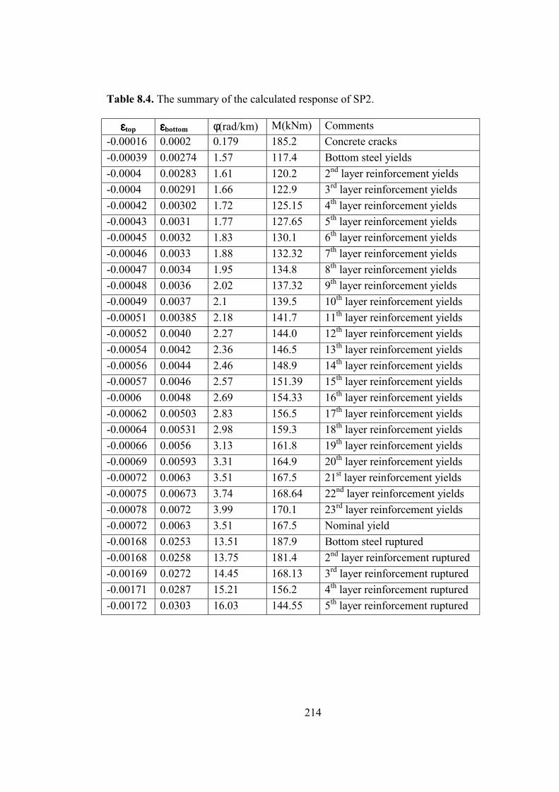
214
Table 8.4. The summary of the calculated response of SP2.
εεεεtop εεεεbottom φ(rad/km) M(kNm) Comments -0.00016 0.0002 0.179 185.2 Concrete cracks -0.00039 0.00274 1.57 117.4 Bottom steel yields -0.0004 0.00283 1.61 120.2 2nd layer reinforcement yields -0.0004 0.00291 1.66 122.9 3rd layer reinforcement yields -0.00042 0.00302 1.72 125.15 4th layer reinforcement yields -0.00043 0.0031 1.77 127.65 5th layer reinforcement yields -0.00045 0.0032 1.83 130.1 6th layer reinforcement yields -0.00046 0.0033 1.88 132.32 7th layer reinforcement yields -0.00047 0.0034 1.95 134.8 8th layer reinforcement yields -0.00048 0.0036 2.02 137.32 9th layer reinforcement yields -0.00049 0.0037 2.1 139.5 10th layer reinforcement yields -0.00051 0.00385 2.18 141.7 11th layer reinforcement yields -0.00052 0.0040 2.27 144.0 12th layer reinforcement yields -0.00054 0.0042 2.36 146.5 13th layer reinforcement yields -0.00056 0.0044 2.46 148.9 14th layer reinforcement yields -0.00057 0.0046 2.57 151.39 15th layer reinforcement yields -0.0006 0.0048 2.69 154.33 16th layer reinforcement yields -0.00062 0.00503 2.83 156.5 17th layer reinforcement yields -0.00064 0.00531 2.98 159.3 18th layer reinforcement yields -0.00066 0.0056 3.13 161.8 19th layer reinforcement yields -0.00069 0.00593 3.31 164.9 20th layer reinforcement yields -0.00072 0.0063 3.51 167.5 21st layer reinforcement yields -0.00075 0.00673 3.74 168.64 22nd layer reinforcement yields -0.00078 0.0072 3.99 170.1 23rd layer reinforcement yields -0.00072 0.0063 3.51 167.5 Nominal yield -0.00168 0.0253 13.51 187.9 Bottom steel ruptured -0.00168 0.0258 13.75 181.4 2nd layer reinforcement ruptured -0.00169 0.0272 14.45 168.13 3rd layer reinforcement ruptured -0.00171 0.0287 15.21 156.2 4th layer reinforcement ruptured -0.00172 0.0303 16.03 144.55 5th layer reinforcement ruptured

215
The curvature ductility ratio for SP2 was found after calculations as 3.85. As
soon as the concrete cracks, the longitudinal reinforcements in the tension side yield
consecutively. The yield moment was found as My = 117.4 kNm, the ratio of yield
moment to cracking moment is calculated as 0.634. Ultimate moment is 187.9 kN
and the ratio of the ultimate moment to the cracking moment after calculations is
found to be 0.507. The curvature ductility ratio for SP2 was calculated as .85.3=µφ
From the observations of the moment-curvature relationship of SP2 the
following conclusions can be drawn:
• The panel form test specimen SP2 reaches their ultimate strength as soon as
the concrete cracks; followed by immediate yielding and rupturing of the
longitudinal steel in the tension side of the wall.
• From the results of the moment curvature relationship, SP2 shows very brittle
behavior due to under-reinforcement. From the results of the moment-
curvature relationship, the ratio of the ultimate moment to the cracking
moment is smaller than 1.25.
8.13 EFFECTS OF TACK WELDING ON SP2
8.13.1 Ductility Reduction
Ultimate strain of the reinforcing steel is changed and the moment-curvature
diagrams are drawn. The effect of ultimate strain of reinforcing steel on the moment-
curvature behavior of SP2 is shown in Figure 8.24. The moment-curvature diagram
of SP2 is drawn by taking the same εsu values used for SP1. From the moment
curvature diagram, it is seen that the cracking moment is 185 kNm. Slight increase is
observed at the moment capacity while increasing the ultimate strain of the
longitudinal steel. The ultimate moment capacity in all cases is approximately
188 kNm. The ratio of the cracking moment to the ultimate moment is 1.016 and it is
smaller than 1.25 for this case as in SP1. When the rupture strain of reinforcing steel
is changed from 0.01 to 0.05, the moment-curvature behavior does not change as
seen in Figure 8.24.

216
Figure 8.24 Effect of ultimate strain of reinforcing steel on the moment-curvature
behavior of SP2.
8.13.2 Strength Reduction
Figure 8.25 shows the effect of ultimate stress of reinforcing steel on the
moment-curvature behavior of SP2. As was done for SP1, the ultimate strength of the
reinforcing steel was changed and it was seen that the general behavior did not
change as seen in the results of SP1.
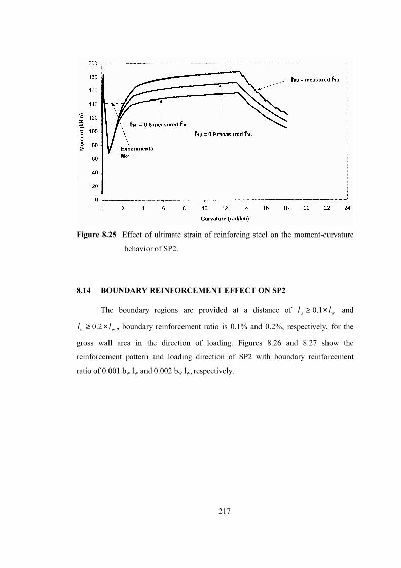
217
Figure 8.25 Effect of ultimate strain of reinforcing steel on the moment-curvature
behavior of SP2.
8.14 BOUNDARY REINFORCEMENT EFFECT ON SP2
The boundary regions are provided at a distance of wu 1.0 ll ×≥ and
wu 2.0 ll ×≥ , boundary reinforcement ratio is 0.1% and 0.2%, respectively, for the
gross wall area in the direction of loading. Figures 8.26 and 8.27 show the
reinforcement pattern and loading direction of SP2 with boundary reinforcement
ratio of 0.001 bw lw and 0.002 bw lw, respectively.

218
SP2Loadingdirection
Fρb = 0.001 bw lw
lb > 0.1 lw = 230 mm
Figure 8.26 Reinforcement pattern and loading direction of SP2 with boundary
reinforcement ratio of 0.001 bw lw.
SP2Loadingdirection
Flb > 0.2 lw = 430 mm
ρb = 0.002 bw lw
Figure 8.27 Reinforcement pattern and loading direction of SP2 with boundary
reinforcement ratio of 0.002 bw lw.

219
Figure 8.28 Comparison of the moment-curvature diagram by providing
concentrated boundary reinforcement.
Three cases are compared in Figure 8.28. The moment-curvature curve at the
top shows the concentrated boundary reinforcement is provided at a distance of
wu 2.0 ll ×≥ . In this case the ultimate moment is greater than 1.25 Mcr. The behavior
in this case is different from the test specimen behavior. When the rupture strain of
the mesh reinforcement reaches its rupture value, mesh reinforcement starts to
rupture. The crushing of concrete is observed.
8.15 COMPARISONS OF THE LOAD-DISPLACEMENT CURVES AND
RESPONSE ENVELOPE CURVES
Comparison of the lateral load displacement curve of SP1 and SP2 for the 1st,
2nd, 3rd and 4th stories are shown in Figures 8.29, 8.30, 8.31 and 8.32. The load
carrying capacity of SP2 is two times greater than SP1. SP1 shows more ductile
behavior when compared with SP2.
0
50
100
150
200
250
300
350
400
450
0 5 10 15 20 25 30 35 40 45 50
Curvature (rad/km)
Mom
ent (
kNm
)
ρρρρb = 0.001bwlwlb = 0.1 lw
ρρρρb = 0.002bwlwlb = 0.2 lw
ρρρρb = 0lb = 0

220
Figure 8.29 Comparison of the lateral load displacement curves of SP1 and SP2 for
the 1st story.
Figure 8.30 Comparison of the lateral load displacement curves of SP1 and SP2 for
the 2nd story.

221
Figure 8.31 Comparison of the lateral load displacement curves of SP1 and SP2 for
the 3rd story.
Figure 8.32 Comparison of the lateral load displacement curves of SP1 and SP2 for
the 4th story.
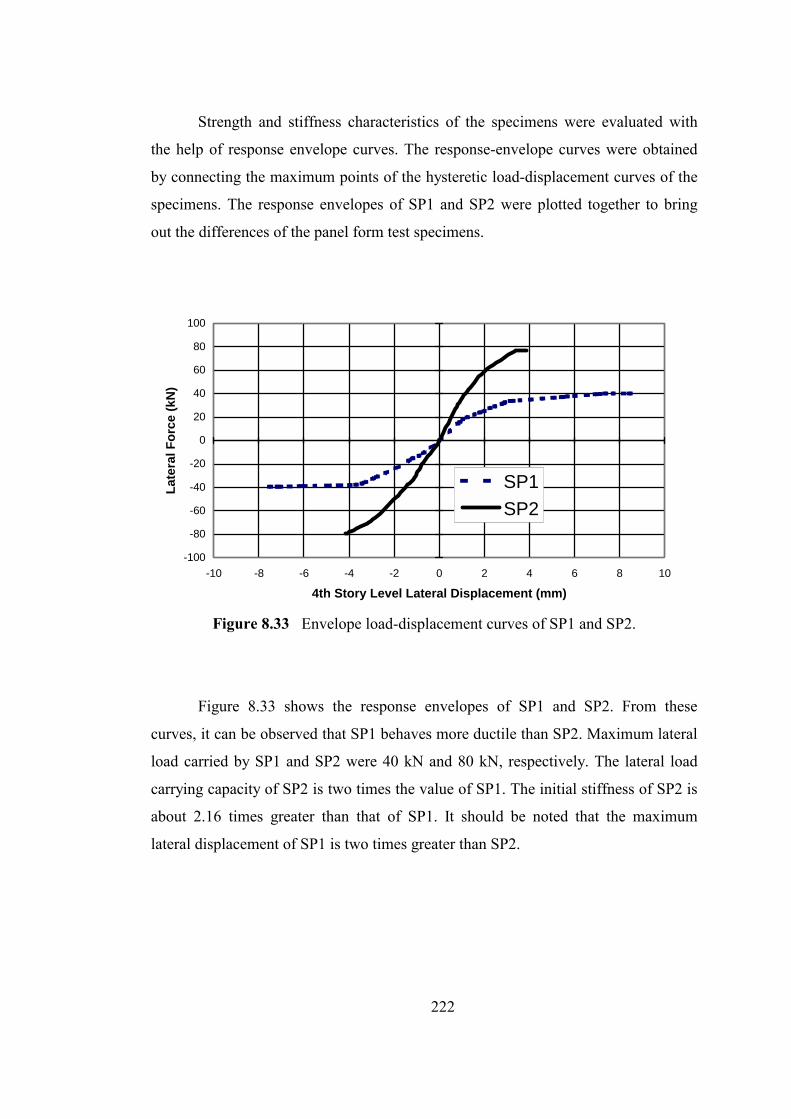
222
Strength and stiffness characteristics of the specimens were evaluated with
the help of response envelope curves. The response-envelope curves were obtained
by connecting the maximum points of the hysteretic load-displacement curves of the
specimens. The response envelopes of SP1 and SP2 were plotted together to bring
out the differences of the panel form test specimens.
-100
-80
-60
-40
-20
0
20
40
60
80
100
-10 -8 -6 -4 -2 0 2 4 6 8 10
4th Story Level Lateral Displacement (mm)
Late
ral F
orce
(kN
)
SP1SP2
Figure 8.33 Envelope load-displacement curves of SP1 and SP2.
Figure 8.33 shows the response envelopes of SP1 and SP2. From these
curves, it can be observed that SP1 behaves more ductile than SP2. Maximum lateral
load carried by SP1 and SP2 were 40 kN and 80 kN, respectively. The lateral load
carrying capacity of SP2 is two times the value of SP1. The initial stiffness of SP2 is
about 2.16 times greater than that of SP1. It should be noted that the maximum
lateral displacement of SP1 is two times greater than SP2.
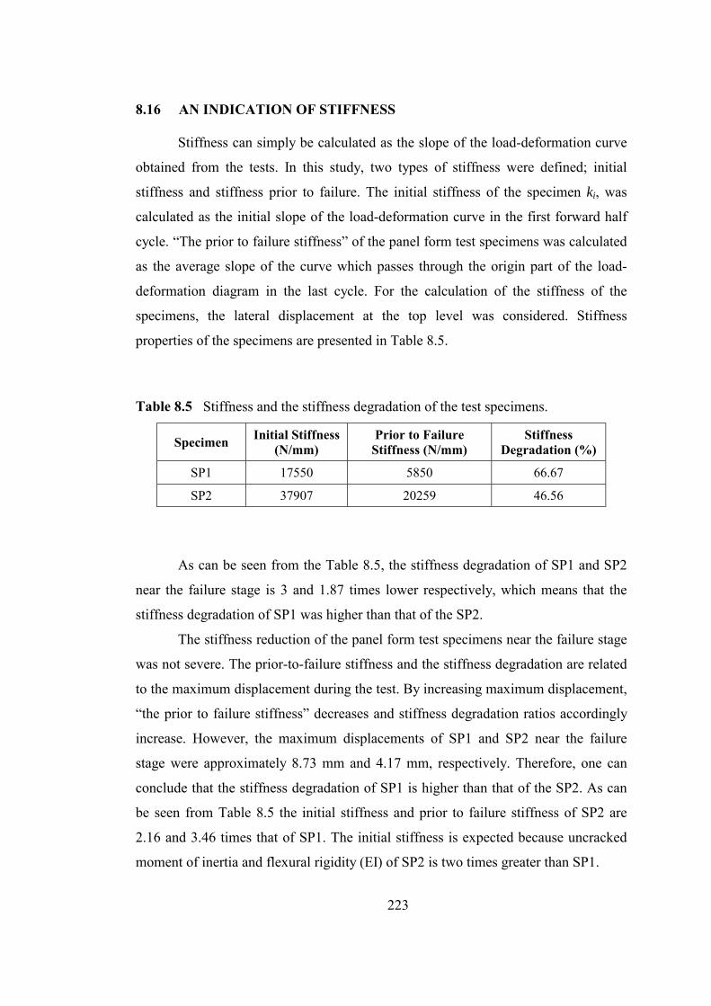
223
8.16 AN INDICATION OF STIFFNESS
Stiffness can simply be calculated as the slope of the load-deformation curve
obtained from the tests. In this study, two types of stiffness were defined; initial
stiffness and stiffness prior to failure. The initial stiffness of the specimen ki, was
calculated as the initial slope of the load-deformation curve in the first forward half
cycle. “The prior to failure stiffness” of the panel form test specimens was calculated
as the average slope of the curve which passes through the origin part of the load-
deformation diagram in the last cycle. For the calculation of the stiffness of the
specimens, the lateral displacement at the top level was considered. Stiffness
properties of the specimens are presented in Table 8.5.
Table 8.5 Stiffness and the stiffness degradation of the test specimens.
Specimen Initial Stiffness (N/mm)
Prior to Failure Stiffness (N/mm)
Stiffness Degradation (%)
SP1 17550 5850 66.67
SP2 37907 20259 46.56
As can be seen from the Table 8.5, the stiffness degradation of SP1 and SP2
near the failure stage is 3 and 1.87 times lower respectively, which means that the
stiffness degradation of SP1 was higher than that of the SP2.
The stiffness reduction of the panel form test specimens near the failure stage
was not severe. The prior-to-failure stiffness and the stiffness degradation are related
to the maximum displacement during the test. By increasing maximum displacement,
“the prior to failure stiffness” decreases and stiffness degradation ratios accordingly
increase. However, the maximum displacements of SP1 and SP2 near the failure
stage were approximately 8.73 mm and 4.17 mm, respectively. Therefore, one can
conclude that the stiffness degradation of SP1 is higher than that of the SP2. As can
be seen from Table 8.5 the initial stiffness and prior to failure stiffness of SP2 are
2.16 and 3.46 times that of SP1. The initial stiffness is expected because uncracked
moment of inertia and flexural rigidity (EI) of SP2 is two times greater than SP1.

224
8.17 ENERGY DISSIPATION
The amount of dissipated energy in the specimens was calculated as the area
under the experimental load-deformation curves. The work done by the axial load
and the energy dissipated by means of the friction forces were neglected since they
were small.
The energy dissipation characteristics of the specimens strongly depend on
the loading history. Therefore, it would be more meaningful to compare the energy
dissipation characteristics of specimens with the same loading history. However, in
this experimental study presented in this thesis, the loading histories of SP1 and SP2
were different.
The cumulative displacement was calculated as the addition of absolute
maximum displacements in the forward half and backward half cycles
(Canbay, 2001). Figure 8.34 shows the cumulative energy dissipation curves of SP1
for the first and second static tests. As can be seen from the Figure 8.34, SP1
dissipated more energy in the 2nd static test as compared to the 1st static test, because
the 1st static test was in the elastic range, and the 2nd static test was in the nonlinear
range. Figure 8.35 shows the cumulative energy dissipation curves of the static tests
of SP1.

225
Table 8.6 Summary of the absolute cumulative displacement and cumulative energy
dissipation of the first test of SP1.
Half cycle No
Maximum top displ.
(mm)
Lateral load (kN)
Absolute cumulative
displacement (mm)
Energy per
cycle (kNmm)
Cumulative energy
(kNmm)
1
-1
2
-2
3
-3
4
-4
5
-5
1.27
-1.46
1.40
-1.52
1.96
-2.00
2.53
-2.66
3.89
-4.60
20
-20
20
-20
25
-25
30
-30
35
-35
1.27
2.73
4.13
5.65
7.61
9.61
12.14
14.8
18.69
23.29
12.7
14.6
14.0
15.2
24.5
25.0
37.95
39.9
77.0
98.0
12.7
27.3
41.3
56.2
81
106
143.9
181.9
258.9
356.9
Table 8.7 Summary of the absolute cumulative displacement and cumulative energy
dissipation of the second static test of SP1.
Half cycle No
Maximum top displ.
(mm)
Lateral load (kN)
Absolute cumulative
displacement (mm)
Energy per
cycle (kNmm)
Cumulative energy
(kNmm)
1
-1
2
-2
5.32
-5.37
8.6
-7.3
35
-35
40
-40
5.32
10.69
19.29
26.59
147
157
199
203
147
304
503
706
Figure 8.36 shows the cumulative energy dissipation curves of SP2 for the
first and second static tests. As can be seen from Figure 8.36, SP2 dissipated much
more energy in the 2nd static test as compared to the 1st static test. This is reasonable

226
because in the 1st static test of SP2 maximum applied lateral load was half of the 2nd
static test. Figure 8.37 shows the cumulative energy dissipation curves of the static
tests of SP2. Figure 8.38 shows the cumulative energy dissipation curves of SP1 and
SP2 for the static tests. It is seen from Figure 8.38 that SP1 dissipates more energy
than SP2 in the static tests.
It would be misleading to draw generalized conclusions form Figures 8.34,
8.35, 8.36, 8.37 and 8.38, since the load histories were different.
0
100
200
300
400
500
600
700
800
0 5 10 15 20 25 30
Absolute Cumulative Displacement (mm)
Cum
ulat
ive
Ener
gy (k
N-m
m) First Static Test
Second Static Test
Figure 8.34 Cumulative energy dissipation curves of the SP1 for the first and
second static test.

227
0
200
400
600
800
1000
1200
0 10 20 30 40 50 60Absolute Cumulative Displacement (mm)
Cum
ulat
ive
Ener
gy (k
N-m
m)
Figure 8.35 Cumulative energy dissipation curve of the static tests of SP1.
Table 8.8 Summary of the absolute cumulative displacement and cumulative energy
dissipation of the first static test of SP2.
Half cycle No
Maximum top displ.
(mm)
Lateral load (kN)
Absolute cumulative
displacement (mm)
Energy per
cycle (kNmm)
Cumulative energy
(kNmm)
1
-1
2
-2
3
-3
4
-4
5
-5
0.234
-0.322
0.352
-0.498
0.498
-0.664
0.654
-0.830
0.810
-1.016
10.0
-10.0
15.0
-15.0
20.0
-20.0
25.0
-25.0
30.0
-30.0
0.234
0.556
0.908
1.406
1.904
2.568
3.222
4.052
4.862
5.878
1.170
1.610
2.640
3.735
3.735
6.640
8.175
10.375
12.150
15.240
1.170
2.780
5.420
9.155
12.890
19.530
27.705
38.080
50.230
65.470

228
Table 8.9 Summary of the absolute cumulative displacement and cumulative energy
dissipation of the second static test of SP2.
Half cycle No
Maximum top displ.
(mm)
Lateral load (kN)
Absolute cumulative
displacement (mm)
Energy per
cycle (kNmm)
Cumulative energy
(kNmm)
1
-1
2
-2
3
-3
4
-4
5
-5
0.710
-0.535
1.390
-1.220
-2.195
-1.976
3.080
-2.685
4.100
-3.200
20.0
-20.0
40.0
-40.0
55.0
-55.0
70.0
-70.0
80.0
-80.0
0.710
1.245
2.635
3.885
6.050
8.026
11.106
13.791
17.891
21.091
7.10
5.35
27.80
24.4
60.36
54.34
107.8
93.98
164
117
7.10
12.45
40.25
64.65
125.01
179.35
287.15
381.13
545.13
662.13
0
100
200
300
400
500
600
700
0 5 10 15 20 25Absolute Cumulative Displacement (mm)
Cum
ulat
ive
Ener
gy (k
N-m
m) First Static Test
Second Static Test
Figure 8.36 Cumulative energy dissipation curves of SP2 for the first and second
static tests.
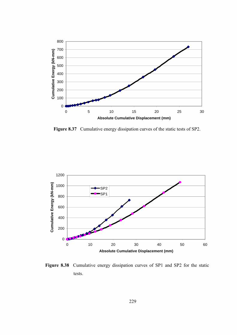
229
0
100
200
300
400
500
600
700
800
0 5 10 15 20 25 30
Absolute Cumulative Displacement (mm)
Cum
ulat
ive
Ener
gy (k
N-m
m)
Figure 8.37 Cumulative energy dissipation curves of the static tests of SP2.
0
200
400
600
800
1000
1200
0 10 20 30 40 50 60
Absolute Cumulative Displacement (mm)
Cum
ulat
ive
Ener
gy (k
N-m
m)
SP2SP1
Figure 8.38 Cumulative energy dissipation curves of SP1 and SP2 for the static
tests.

230
8.18 STORY DRIFT INDEX
Story drift index is defined as the relative displacement between the two
successive floors dividing the corresponding story height and frequently used in
earthquake engineering considering a measure of structural and non-structural
damage. Story drift index is not allowed to exceed a certain limit in order to prevent
structural and non-structural damage. Additionally for interstory drifts more than 1%,
P-∆ effects lead to rapidly increasing augmentation of these drifts (Paulay, 1992).
According to the Turkish Seismic Code (AY, 1997), the maximum story drift index
is limited to 0.0035 and 0.02/R based on the elastic analysis of the structure. R is the
behavior factor and for shear wall structures of normal ductility R = 4. On the other
hand, according to (UBC 1997), the maximum story drift index for inelastic analysis
is limited to 0.025 for the structures with a fundamental period less than 0.7 seconds,
and 0.02 for the structures with a fundamental period greater than 0.7 seconds. As the
numbers indicate, the Turkish Seismic Code is more conservative about the amount
of story drift index.
Figures 8.39, 8.40, 8.41, and 8.42 show envelope curves of the 1st, 2nd, 3rd and
4th story drift ratios for SP1.
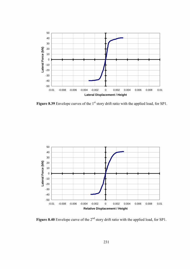
231
-50
-40
-30
-20
-10
0
10
20
30
40
50
-0.01 -0.008 -0.006 -0.004 -0.002 0 0.002 0.004 0.006 0.008 0.01
Lateral Displacement / Height
Late
ral F
orce
(kN
)
Figure 8.39 Envelope curves of the 1st story drift ratio with the applied load, for SP1.
-50
-40
-30
-20
-10
0
10
20
30
40
50
-0.01 -0.008 -0.006 -0.004 -0.002 0 0.002 0.004 0.006 0.008 0.01
Relative Displacement / Height
Late
ral F
orce
(kN
)
Figure 8.40 Envelope curve of the 2nd story drift ratio with the applied load, for SP1.
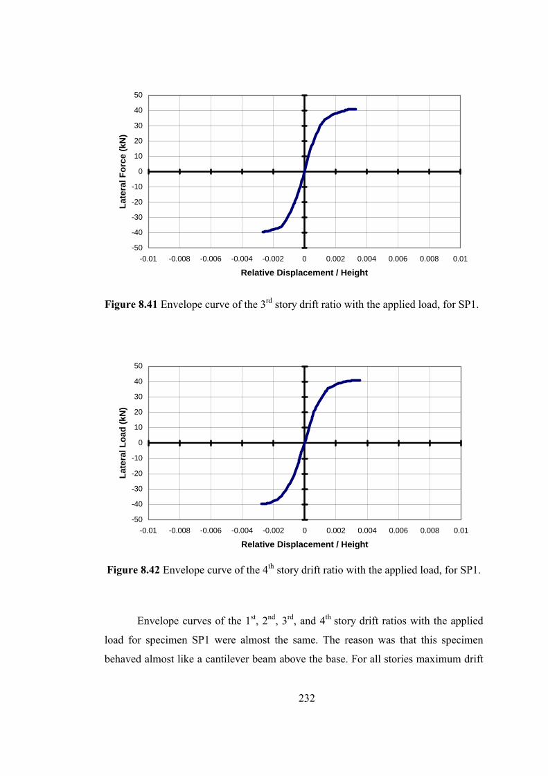
232
-50
-40
-30
-20
-10
0
10
20
30
40
50
-0.01 -0.008 -0.006 -0.004 -0.002 0 0.002 0.004 0.006 0.008 0.01
Relative Displacement / Height
Late
ral F
orce
(kN
)
Figure 8.41 Envelope curve of the 3rd story drift ratio with the applied load, for SP1.
-50
-40
-30
-20
-10
0
10
20
30
40
50
-0.01 -0.008 -0.006 -0.004 -0.002 0 0.002 0.004 0.006 0.008 0.01
Relative Displacement / Height
Late
ral L
oad
(kN
)
Figure 8.42 Envelope curve of the 4th story drift ratio with the applied load, for SP1.
Envelope curves of the 1st, 2nd, 3rd, and 4th story drift ratios with the applied
load for specimen SP1 were almost the same. The reason was that this specimen
behaved almost like a cantilever beam above the base. For all stories maximum drift
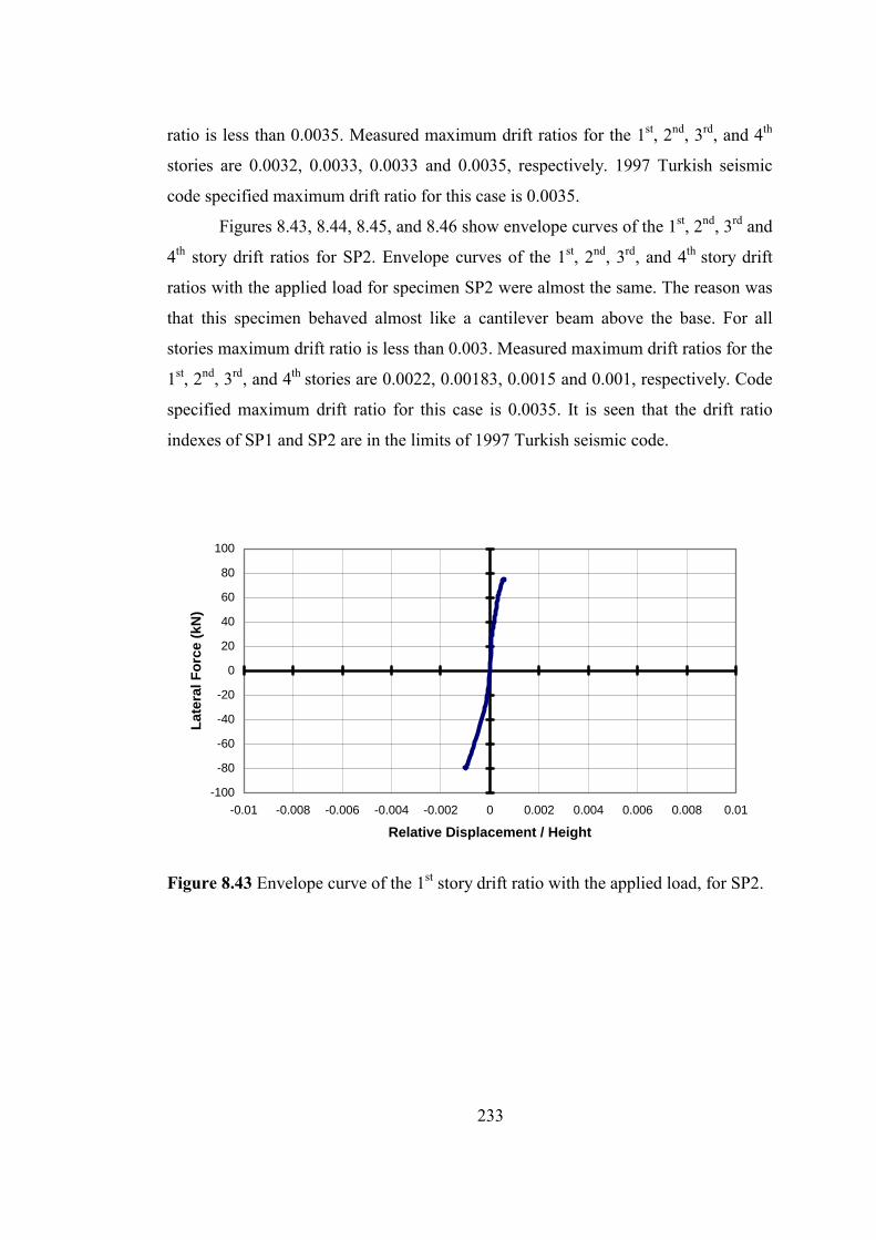
233
ratio is less than 0.0035. Measured maximum drift ratios for the 1st, 2nd, 3rd, and 4th
stories are 0.0032, 0.0033, 0.0033 and 0.0035, respectively. 1997 Turkish seismic
code specified maximum drift ratio for this case is 0.0035.
Figures 8.43, 8.44, 8.45, and 8.46 show envelope curves of the 1st, 2nd, 3rd and
4th story drift ratios for SP2. Envelope curves of the 1st, 2nd, 3rd, and 4th story drift
ratios with the applied load for specimen SP2 were almost the same. The reason was
that this specimen behaved almost like a cantilever beam above the base. For all
stories maximum drift ratio is less than 0.003. Measured maximum drift ratios for the
1st, 2nd, 3rd, and 4th stories are 0.0022, 0.00183, 0.0015 and 0.001, respectively. Code
specified maximum drift ratio for this case is 0.0035. It is seen that the drift ratio
indexes of SP1 and SP2 are in the limits of 1997 Turkish seismic code.
-100
-80
-60
-40
-20
0
20
40
60
80
100
-0.01 -0.008 -0.006 -0.004 -0.002 0 0.002 0.004 0.006 0.008 0.01
Relative Displacement / Height
Late
ral F
orce
(kN
)
Figure 8.43 Envelope curve of the 1st story drift ratio with the applied load, for SP2.
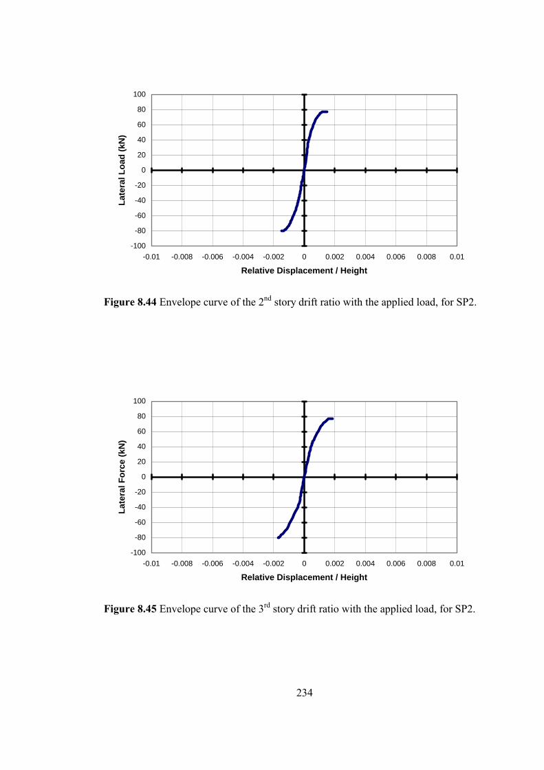
234
-100
-80
-60
-40
-20
0
20
40
60
80
100
-0.01 -0.008 -0.006 -0.004 -0.002 0 0.002 0.004 0.006 0.008 0.01
Relative Displacement / Height
Late
ral L
oad
(kN
)
Figure 8.44 Envelope curve of the 2nd story drift ratio with the applied load, for SP2.
-100
-80
-60
-40
-20
0
20
40
60
80
100
-0.01 -0.008 -0.006 -0.004 -0.002 0 0.002 0.004 0.006 0.008 0.01
Relative Displacement / Height
Late
ral F
orce
(kN
)
Figure 8.45 Envelope curve of the 3rd story drift ratio with the applied load, for SP2.
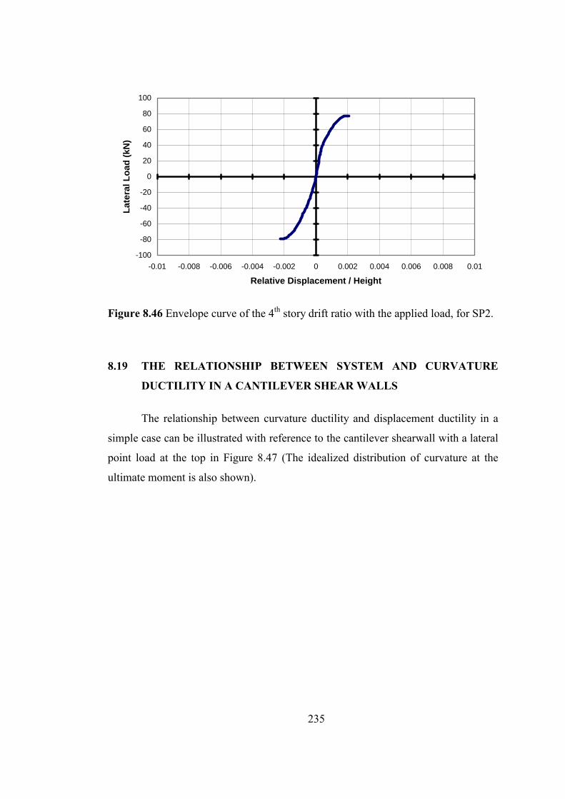
235
-100
-80
-60
-40
-20
0
20
40
60
80
100
-0.01 -0.008 -0.006 -0.004 -0.002 0 0.002 0.004 0.006 0.008 0.01
Relative Displacement / Height
Late
ral L
oad
(kN
)
Figure 8.46 Envelope curve of the 4th story drift ratio with the applied load, for SP2.
8.19 THE RELATIONSHIP BETWEEN SYSTEM AND CURVATURE
DUCTILITY IN A CANTILEVER SHEAR WALLS
The relationship between curvature ductility and displacement ductility in a
simple case can be illustrated with reference to the cantilever shearwall with a lateral
point load at the top in Figure 8.47 (The idealized distribution of curvature at the
ultimate moment is also shown).

236
Figure 8.47 Cantilever shear wall with lateral loading at ultimate moment
The lateral yield deflection at the top of the shear wall ∆y is
3H2
yy
×φ=∆ (8.6)
The plastic hinge rotation θp may be assumed to result from uniform plastic
curvature φp in the plastic hinge length p! shown in Figure 8.47, so that
( ) pyuppp !! ×φ−φ=×φ=θ (8.7)
Assuming the plastic rotation to be concentrated at midheight of the plastic
hinge, the plastic displacement at the top of the shear wall can be calculated by using
Equation 8.8.
( ) ( ) ( )ppyuppp 5.0H5.0H !!! ×−××φ−φ=×−×θ=∆ (8.8)

237
The system or displacement ductility for the cantilever shear wall was
previously defined as
y
p
y
py
y
u 1∆∆
+=∆
∆+∆=
∆∆
=µ∆ (8.9)
Substituting Equations (8.6) and (8.8) into Equation (8.9) and rearranging
yields the relationship between displacement and curvature ductility as in Equation
(8.10)
( )
×
−××−µ×+=µ φ∆ H21
H131 pp !!
(8.10)
or conversely,
( )
×
−×
×
−µ+=µ ∆
φ
H21
H3
11
pp !! (8.11)
Paulay and Priestly (1991) suggest two alternative expressions for the plastic
hinge length:
H03.02.0 wp ×+×= !! (8.12)
yblp fd022.0H0536.0 ××+×=! (8.13)
Equation 8.12 includes w! to the estimate of plastic hinge to account for the
influence of plasticity spread due to diagonal cracking. It is felt to be more
appropriate for squat walls. Equation 8.13, which was originally developed for
columns, is more strongly related to wall height, and includes a term for strain
penetration into the foundation, which is depended on diameter dbl and yield strength
fy of the longitudinal reinforcement, and should be more appropriate at higher aspect
ratios. Therefore, for the panel form test specimens SP1 and SP2 the plastic hinge
length is calculated as follows:
mm170mm31.1675502022.026700536.0p ≈=××+×=!
238
8.20 The Relationship Between System and Curvature Ductility for SP1
By using mm170p =! and H = 2670 mm and curvature ductility ratio
89.7=µφ (from the moment curvature relation obtained from Waller2002 and
Response2000) the displacement ductility factor can be found as
( ) ( )
×−××−×+=
×
−××−µ×+=µ φ∆ 267021701
2670170189.731
H21
H131 pp !!
54)required(274.2)found( ≈=µ<=µ ∆∆
It is understood from the above equation that SP1 does not have enough
displacement ductility.
By assuming that SP1 has displacement ductility 4=µ∆ , we can find the
required curvature ductility and compare it with the available curvature ductility
found from Waller2002.
( ) ( )
×−×
×
−+=
×
−×
×
−µ+=µ ∆
φ
267021701
26701703
141
H21
H3
11
pp !!
89.7)found(23.17)required( =µ>=µ φφ
Curvature ductility of SP1 was found as µφ = 7.89 form the computer
programs Waller2002 and Response-2000. The required curvature ductility is 2.18
times greater than the available curvature ductility. It is obvious that SP1 does not
have enough curvature ductility capacity either.
8.21 The Relationship Between System and Curvature Ductility for SP2
The displacement ductility factor can be found by using mm170p =! and H
= 2670 mm and curvature ductility ratio 85.3=µφ (from the moment curvature
relation obtained from Waller2002 and Response2000).
239
( ) ( )
×−××−×+=
×
−××−µ×+=µ φ∆ 267021701
2670170185.331
H21
H131 pp !!
54)required(527.1)found( ≈=µ<=µ ∆∆
SP2 has very limited displacement ductility capacity. Displacement ductility
of SP2 is smaller than SP1 as observed from the static tests of SP1 and SP2.
By assuming that SP2 has displacement ductility 4=µ∆ , we can find the
required curvature ductility and compare it with the available curvature ductility
found from Waller2002.
( ) ( )
×−×
×
−+=
×
−×
×
−µ+=µ ∆
φ
267021701
26701703
141
H21
H3
11
pp !!
85.3)found(23.17)required( =µ>=µ φφ
Curvature ductility of SP1 was found as µφ = 3.85 from the moment curvature
diagram obtained from the computer programs Waller2002 and Response-2000. It is
obvious from the above equation that SP2 has very limited curvature ductility
capacity. This brittle behavior is also observed in the static tests of SP2.
It is obvious from the above calculations that the panel form test specimens
SP1 and SP2 do not have enough curvature ductility and displacement ductility.
Panel form test specimens, subject to reversed loading that causes tension cracking of
the concrete, behave in a brittle manner, and thus, do not seem to be earthquake-safe.
8.22 DISPLACEMENT DUCTILITY FACTOR FROM THE ENVELOPE
CURVES
The displacement ductility factor μ∆ is mostly used in the seismic design
codes. It has also been called the “global ductility factor” in some publications, since
it describes the extent of the post elastic displacement of a whole structure. Figures
8.48 and 8.49 show the envelope curves of the top displacement with the applied
load for SP1 and SP2, respectively.
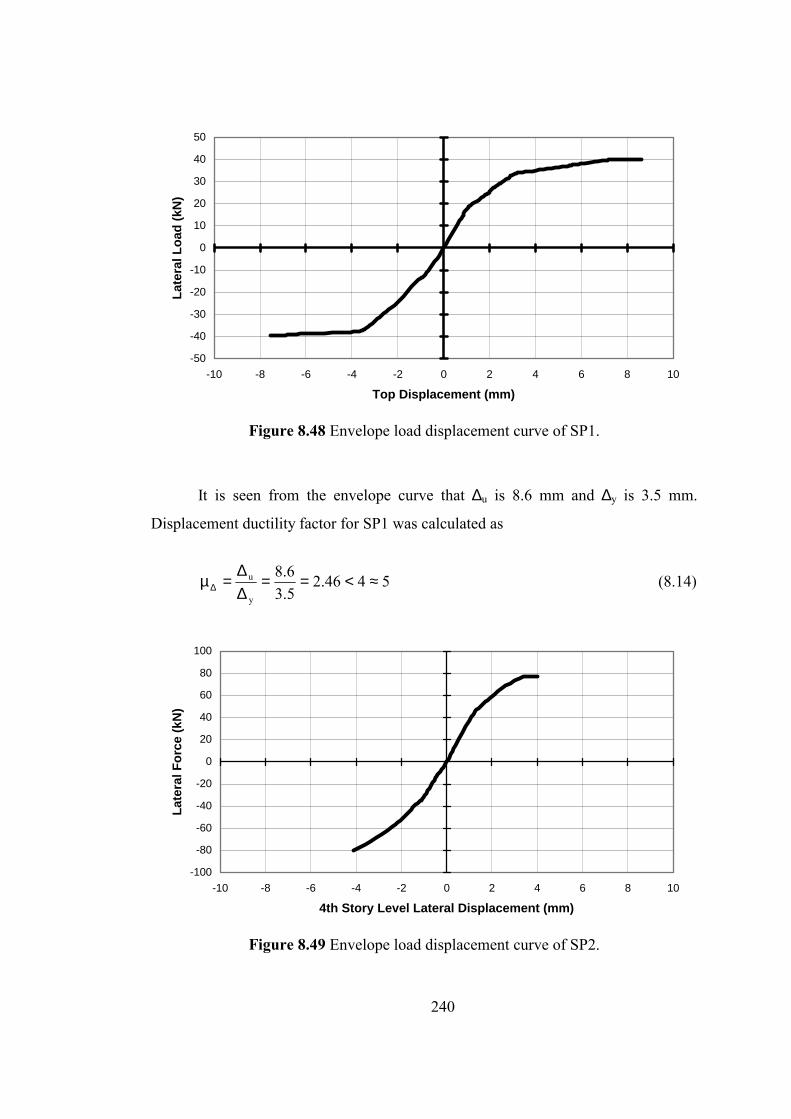
240
-50
-40
-30
-20
-10
0
10
20
30
40
50
-10 -8 -6 -4 -2 0 2 4 6 8 10
Top Displacement (mm)
Late
ral L
oad
(kN
)
Figure 8.48 Envelope load displacement curve of SP1.
It is seen from the envelope curve that ∆u is 8.6 mm and ∆y is 3.5 mm.
Displacement ductility factor for SP1 was calculated as
5446.25.36.8
y
u ≈<==∆∆
=µ∆ (8.14)
-100
-80
-60
-40
-20
0
20
40
60
80
100
-10 -8 -6 -4 -2 0 2 4 6 8 10
4th Story Level Lateral Displacement (mm)
Late
ral F
orce
(kN
)
Figure 8.49 Envelope load displacement curve of SP2.

241
It is seen from the envelope curve that ∆u is 4.13 mm and ∆y is 2.67 mm.
Displacement ductility factor for SP2 was calculated as
5455.167.213.4
y
u ≈<==∆∆
=µ∆ (8.15)
It can be concluded that from the Equation 8.14, Equation 8.15 and also
Sections 8.20 and 8.21 both SP1 and SP2 show very brittle behavior due to
under-reinforcement. Panel form structures possess potential brittleness when subject
to earthquake loading. This brittleness springs from excessively low under-
reinforcement.
242
CHAPTER 9
CONCLUSIONS AND RECOMMENDATIONS
9.1 CONCLUSIONS
1) Multi-story panel buildings (buildings built by tunnel-form) which were
constructed before the Turkish Earthquake Code (AY-1997) was published are
subject to severe earthquake risks of failing in a brittle mode.
2) The risk of failing in a brittle mode springs from the fact that the longitudinal steel
ratio is very low as ρsv = 0.0015.
In the Turkish Earthquake Code (AY-1997), for structures in which the total
earthquake force is carried by shear walls, the longitudinal steel ratio can be reduced
to ρsv = 0.0015 from ρsv = 0.0025, which is the normal minimum.
3) The standard practice in structures built by tunnel-form is to use mesh
reinforcement to provide longitudinal steel ratio of ρsv = 0.0015. Before the
publication of (AY-1997), no end zones in walls were formed.
4) The brittle failure occurs due to the big difference between the moment
corresponding to the tension cracking of concrete and the ultimate moment provided
by the longitudinal steel
Mcr >> Mu
As soon as cracking occurs, concrete can carry no tension force. This tension
force is unloaded to the tension steel. The minimum amount of longitudinal steel
(ρsv = 0.0015) cannot carry the unloaded tension force. It immediately yields and

243
elongates until rupture. The result is a brittle failure.
5) As reinforced by ρsv = 0.0015, the tunnel-form units dissipates very small amount
of earthquake energy.
6) Addition of steel to the end of wall cross-section and forming end zones, as
required by Turkish Earthquake Code (AY-1997) improves the failure behavior to
acceptable standards.
7) In the cross-section of the test unit, as reinforced according to Turkish Earthquake
Code (AY-1997)
Ultimate moment capacity of the cracked cross-section is greater than the
moment corresponding to the tension cracking of concrete
Mu >> Mcr
The failure mode of the cross-section with end zones is ductile.
8) The effect of tack welding on the failure mode is investigated and found to be
insignificant in the brittle failure mode.
9) Tension tests of the 2 mm diameter wires used as reinforcement are performed
before and after tack welding. Approximately the same failure loads are found (10%
difference). Additionally, the rupture points on the tack-welded wire are almost never
exactly on the tack welding. The rupture points occur at some distance away from the
tack weld.
10) A special Axial Load-Moment-Curvature (N-M-φ) computer program is
developed theoretically to analyze the experimentally tested tunnel form units.
Computer analyses show the same brittle failure mode, as observed in the laboratory
tests.
11) For considering the possibility of the negative effect of tack welding, by reducing
both the strength and ductility of the reinforcement, the parametric study obtained by
244
both Response-2000 and Waller-2002 (N-M-φ) programs produce the same behavior
of brittle failure. It is interesting to note that, the same brittle failure behavior would
occur, even if the ultimate strength and ductility of the reinforcing wire were higher.
12) Dynamic tests are performed on panel form units to determine the natural periods
in X and Y directions of the cross-section.
13) The panel form test units are modeled by the computer by using the Finite
Element Technique and the Wide Column Analogy Technique. Theoretical natural
periods are calculated.
14) Experimentally found and theoretically calculated natural periods are almost the
same. This fact proves a very important point that the computer models used
satisfactorily reflect the realistic dynamic behavior of panel structures.
15) The Finite Element Model is commonly accepted to be realistic, but the wide
column analogy is not as readily accepted. The dynamic analysis prove that the wide
column analogy could also determine natural periods very close to the
experimentally found correct values.
The wide column analogy is a very valuable analytical tool for structural
analysis. It reduces the two-dimensional panels to one-dimensional structural
elements. Thus the panel structure can be modeled and analyzed as a framed
structure. The framed structure, of course, is a method of analysis, which the design
engineers are very familiar with.
16) A special purpose computer program is developed (named Waller2002) to
develop the accurate N-M-φ relationship of reinforced concrete cross-sections.
N-M-φ program, known as RESPONSE-2000, exists on the Internet. However, it has
many weaknesses and aspects, which cannot be handled. Waller-2002 is developed
as an improvement of the program RESPONSE-2002.
245
17) From the observations of the moment-curvature relationship of panel form test
specimens, they have reached their ultimate strength as soon as the concrete cracked;
followed by immediate yielding and then rupturing of the longitudinal steel.
Subject to an earthquake, the panel walls initially exhibit tension cracking of
the concrete. The unloaded moment after tension cracking immediately makes the
reinforcement yield.
Rapid unloading of the moment after tension cracking of concrete is
terminated by fracture of the distributed longitudinal steel. After longitudinal
reinforcement fractures, moment carrying capacity of the wall section is totally lost.
18) From the moment-curvature relationship, which is obtained by Waller2002, the
panel form test specimens SP1 and SP2 show very brittle behavior. From the results
of the moment-curvature relationship, the ratio of the ultimate moment to the
cracking moment is much smaller than 1.25 for both SP1 and SP2. This is an
indication of very brittle type of behavior of SP1 and SP2.
19) The failure of SP1 and SP2 provides convincing field evidence that brittleness of
reinforced concrete members caused by excessive under-reinforcement cannot be
ignored when designing for seismic resistance.
20) Panel structures (buildings built by tunnel-form) possess potential brittleness
when subject to earthquake loading. This brittleness springs from excessively low
under-reinforcement.
21) Panel buildings, subject to earthquake excitation that causes tension cracking of
the concrete, behave in a brittle manner, and thus, do not seem to be earthquake-safe.
22) It should be made as a Turkish Earthquake Code (AY-1997) requirement that,
the ultimate moment capacity of a shear wall Mu, be at least 1.25 times greater than
the moment that corresponds to concrete cracking, Mcr. A similar regulation occurs
for prestressed concrete beams: Mu > 1.25 Mcr.

246
9.2 RECOMMENDATIONS
Almost no structural damage was reported on buildings built by tunnel-form
in the Marmara Earthquake (1999).
However, the peak ground accelerations in the Marmara Earthquake were
rather small as 0.4g-0.43g. As a result, small inertia forces were generated. On the
other hand, ground displacements were very large, in the order of 2.5-3.0 m.
If an earthquake producing greater ground accelerations occurs, what is the
seismic safety of tunnel-formed structures with walls containing no specially
reinforced end zones?
1) Three-dimensional computer models of different panel buildings, which exist in
practice, should be developed and be subjected to dynamic analysis according to AY-
1997.
2) Each panel should be checked for concrete cracking.
3) N-M-φ relationships of panels should be developed by the computer program
Waller-2002.
4) The possibility of the occurrence of brittle failure must be carefully investigated.
5) Methods of seismic strengthening must be developed to bypass the occurrence of
brittle failure. The developed strengthening method must enable the panel building to
dissipate seismic energy.
6) A detailed and organized program of analysis should be done to determine the
minimum reinforcement requirements of panels in buildings built by tunnel-form
structures. This analytical study must cover all possible wall designs.
7) The minimum reinforcement requirements focusing on amount and distribution of
steel within the cross-sections should be experimentally tested to provide the validity
of the analytical relationships developed.

247
8) Providing end zones in tunnel form units increase the ultimate moment capacity
Mu as
Mu > 1.25 Mcr
In doing so, the lateral force, which the unit is subjected, to also increases. It
should be verified experimentally that the increased lateral force does not lead to a
premature occurrence of shear failure.
9) The effect of wall design geometry should be investigated.
10) Minimum reinforcement amount and distribution of the boundary reinforcement
should be investigated for different wall design geometries.
11) The axial load level of the panel form test specimens should be increased.
12) In this study, H wall design that is numbered as 1 was tested under reversed
lateral loading. Typical wall design geometry that is shown in Figure 9.1 as 2, 3 and
4 should be tested under reversed cyclic lateral loading.
Figure 9.1 Panel form test specimens wall geometry.

248
13) Energy dissipation requirements should be determined for typical floor plans and
height of the buildings.
14) In this study 1/5 scale panel form test specimens were constructed. Such a small
scale caused local construction mistakes. The scale should be increased.

249
REFERENCES
ACI-318 (1971), “Building Code Requirements for Reinforced Concrete,” American
Concrete Institute, Detroit, Michigan, 1971.
ACI-318 (1977), “Building Code Requirements for Reinforced Concrete,” American
Concrete Institute, Detroit, Michigan.
ACI-318 (1983), “Building Code Requirements for Reinforced Concrete,” American
Concrete Institute, Detroit, Michigan.
Aktan, A. E., Bertero V. V., (1985) “Structural Walls: Seismic Design for Shear”
ASCE Journal of Structural Engineering V.111, No.8, August, 1985.
Atımtay, E., (1991) “Seismic design of bridges to relate ductility and sway”
Evaluation and Rehabilitation of Concrete Structures and Innovations in Design,
American Concrete Institute, SP-128.
Atımtay, E., Tuna, M.E. (2001) “Designing the concrete dual system” Structural
Engineering, Mechanics and Computation Vol.2, pp. 1009-1015.
Atımtay, E., (2003) “Tünel kalıplı Yüksek Binaların Deprem Davranışı ve
Güvenliği” TÜBİTAK, İNTAG Proje No:561, Ankara, 2003.

250
AY-1997, Afet Bölgelerinde Yapılacak Yapılar Hakkında Yönetmelik, (1997), T.C.
Bayındırlık ve İskan Bakanlığı Deprem Araştırma Enstitüsü Başkanlığı, Ankara, 85
pages.
Balkaya, C., Kalkan, E., (2002) “Nonlinear seismic response evaluation of tunnel
form building structures” Computers and Structures V.81, pp. 153-165.
Balkaya, C., Kalkan, E., (2003) “Estimation of fundamental periods of shear-wall
dominant building structures” Earthquake Engineering and Structural Dynamics
V.32, pp. 985-998.
Bentz, E., and Collins, M., 1998, RESPONSE 2000, Version 0.7.5 (Beta) University
of Toronto.
Bertero, V.V., Popov, F.P., Wang, T.V., and Wallenas, T., (1977) “Seismic Design
Implications of Hysteretic Behavior of Reinforced Concrete Structural Walls” 6th
World Conference on Earthquake Engineering, New Delhi, Vol.5, pp. 159-165.
Bertero V. V., EERI M. (1986) “Lessons Learned Recent Earthquakes and Research
and Implications for Earthquake-Resistance Design of Buildings Structures in the
United States” Earthquake Spectra, Vol. 2, No.4, pp. 825-858.
Canbay , E. (2001) “Contribution of RC Infills to the Seismic Behavior of Structural
Systems”, A doctor of Philosophy Thesis in civil Engineering, Middle East Technical
University, December 2001.
Cardenas, A. E., Magura, D.D. (1973), “Strength of high-Rise Shear Walls-
Rectangular Cross Section,” Response of Multistory Concrete structures to Lateral
Forces, SP-36, American Concrete Institute, Detroit, pp. 119-150.
251
Cardenas, A. E., Hanson, J. M., Corley, W.G., and Hognestad E., (1982) “Design
Provisions for Shear Walls” Portland Cement Association, Research and
Development Bulletin RD028.01D, February 25, 1982, U SA.
Chopra, A.K.(1995), Dynamic of Structures, Theory and Applications to Earthquake
Engineering, University of California at Berkeley Prentice Hall, USA.
Clough, R.W., and Penzien, J., (1193) Dynamics of Structures, Mc Graw Hill, New
York, 1993.
Coull, A., and Choudhury, J.R. (1967) “Analysis of Coupled Shear Walls”, ACI
Structural Journal, Vol.64, September 1967, pp. 587-593.
Diker, Y. (2000) “Seismic Analysis and Design of Tunnel Form Buildings”, Master
Thesis Submitted to Graduate School of Natural and Applied Sciences of the Middle
East Technical University, May 2000.
Earthquake Effects on Reinforced Concrete Structures: U.S.-Japan Research, SP-84,
American Concrete Institute, Detroit, 1985, USA.
Elnashai, A.; Pilakoutas, K.; and Ambraseys, N.N., (1990) “ Experimental Behaviour
of Reinforced Concrete Walls under Earthquake Loading,” Earthquake Engineering
and Structural Dynamics, V.19, No.3, Apr 1990.
Ersoy, U., Özcebe, G., (1998) “Sarılmış Betonarme Kesitlerde Moment-Eğrilik
İlişkisi-Analitik Bir İrdeleme”, İMO Teknik Dergi, No. 129, pp. 1779-1827.
Ersoy, U., Özcebe G., 2001, Betonarme, Evrim Yayınevi, Ankara, 818 pp.
Fintel, M. (1991). “Shearwalls-An Answer for Seismic Resistance?“ Concrete.
International, Vol.3, No.7, pp.48-53.
252
Grupta, A., and Rangen, B. V., (1998) “High-Strenght Concrete (HSC) Structural
Walls” ACI Structural Journal, V.95, No.2, March-April, 1998.
Hognestad, E., (1951), A study of combined Bending and axial load in R/C
Members, University of Illinois, Engineering Exp. Sta. Bull., No. 399. pp. 42-65.
Kaya, Y. M., (2000) “Capacity Design Considerations of Tunnel Form Buildings”,
Master Thesis Submitted to Graduate School of Natural and Applied Sciences of the
Middle East Technical University, May 2000.
Kowalsky, M.J., (2001) “RC structural Walls Designed According to UBC and
Displacement-Based Methods” Journal of Structural Engineering, V.127, No. 5,
Paper No. 22137, pp. 506-516.
Lefas, I.; Kostovos, M.D.; and Ambraseys, N.N., (1990) “Behavior of Reinforced
Concrete Structural Walls: Strength, Deformation Characteristics, and Failure
Mechanism,” ACI Structural Journal, V. 87, No.1, Jan.-Feb. 1990, pp. 23-31.
Lomnitz, C. (1970), “ Major Earthquakes and Tsunamis in Chile during the Period
1935 to 1955,” Geologische Rundschau, Vol. 59, No. 3, 1970, pp. 938-960.
Matacchoine, A., (1991), “Equivalent Frame Method Applied to Concrete Shear
Walls”, Concrete International, 65, November, 1991.
Turkish Seismic Code, Ministry of Public Work, Ankara, July 1975.
Park, R., and Paulay, T., (1975) Reinforced Concrete Structures, New York, John
Wiley& Sons.

253
Paulay, T., and Üzümeri, S. M., (1975) “ A Critical Review of the Seismic Design
Provisions for Ductile Shear Walls of the Canadian Code and Commentary,”
Canadian journal of Civil Engineering, Vol.2, No.4 1975, pp. 592-601.
Paulay, T., Earthquake-Resisting Shearwalls (1980) “A New Zealand Design Trend.”
ACI Journal Vol. 77, No. 18, May-June 1980, pp. 144-152.
Paulay, T., Priestley, M.J.N., and Synge, A.J. (1981).”Ductility in Earthquake-
Resisting Squat Shearwalls”. American Concrete Inst. Structural J., Vol. 79, No. 4,
pp. 257-269.
Paulay, T., Priestley, M.J.N., 1992, Seismic Design of Reinforced Concrete and
Masonry Buildings, John Wiley&Sons, Inc., New York, USA, 744pp.
Paulay, T., Priestley M. J. N., (1993) “Stability of Ductile Structural Walls” ACI
Structural Journal, V.90, No.4, July-August, 1993 pp.385-392.
Paulay, T., E., (1999) “Seismic Displacement Compatibility in Mixed Structural
System”, Uğur Ersoy Symposium on Structural Engineering, Procedings, METU-
Department of Civil Engineering, Ankara, Turkey, July 1999. pp: 275-292
Pilakoutas, K., Elnashai, A., (1993) “Interpretation of testing Results for Reinforced
Concrete Panels,” ACI Structural Journal, V.90, No.6, Nov-Dec. 1993, pp. 642-645.
Pilakoutas, K., Elnashai, A., (1995) “Cyclic Behavior of Reinforced Concrete
Cantilever Walls, Part I: Experimental Results,” ACI Structural Journal, V.92, No.3,
May-June 1995, pp. 271-281.
RESPONSE-2000 Reinforced Concrete Sectional Analysis, Response-2k Version
0.8.5.2, Evan C. Bentz and Michael P. Collins, 1999, Canada.
254
Rüsch, H, und Hilsdorf, H., 1963, Verformungseigenschaften von Beton Unter
Zwischen Zugspannangen, Materialprüfungsamt für das Bauwesen der Technischen
Hochschule München, Rep. No. 44.
Saatçioğlu, M. and Ravzi, S.R., 1992, Strength and Ductility of Confined Concrete,
J. Struct. Engrg, ASCE V.118, No. 6, pp. 1590-1607.
Sittipunt, W., and Wood, S.L. (1995). “Influence of Web Reinforcement on the
Cyclic Response of Structural Walls”. American Concrete Ins. Structural J., Vol.92,
No.6, pp.745-756.
Sonuvar, M. O., (2001) “Hysteretic Response of Reinforced Concrete Frames
Repaired by Means of Reinforced Concrete Infills”, A Doctor of Philosophy Thesis
in Civil Engineering, Middle East Technical University, June 2001
Stark, R. (1988), “Evaluation of Strength, Stiffness, and Ductility Requirements of
Reinforced Concrete Structures using Data from Chile (19859 and Michoacan (1985)
Earthquakes.” Ph.D. Thesis, Department of Civil Engineering, University of Illinois,
Urbana.
Subedi, N. K. “RC-Coupled Shear Wall Structures I: (1991) Analysis of Coupling
Beams” ASCE Journal of Structural Engineering V.117, No.3, March, 1991 pp. 667-
680.
Subedi, N. K. (1991) “ RC-Coupled Shear Wall Structures. I: Analysis of Coupling
Beams” ASCE Journal of Structural Engineering V.117, No.3, March, 1991 pp. 681-
698.
Takeda, T., Sözen M. A., and Nielsen, N.N. (1970), “ Reinforced Concrete Response
to Simulated Earthquakes, ” ASCE, Journal of the Structural Division, Vol. 96, No.
ST12, December 1970, pp.2557-2573.

255
Tegos, I.A. and Penelis, G. Gr. (1988) “ Seismic Resistance of Short Columnsand
Coupling Beams Reinforced With Inclined Bars”, ACI Structural Journal V.93, No.6,
November-December, 1988.
Theodosios, P. T., Moretti, M., Bezas, (1996)A. “On the Behavior and Ductility of
Reinforced Concrete Coupling Beams of Shear Walls” ACI Structural Journal V.93,
No.6, November-December, 1996 pp.711-720.
Thomas P., EERI M. (1986) “The Design of Ductile Reinforced Concrete Structural
Walls for Earthquake Resistance” Earthquake Spectra, Vol. 2, No.4, pp. 873-822.
TS-500, (1984) Building Code Requirements for Reinforced Concrete, Turkish
Standards Institution, Ankara, April 1984.
TS-500, (2000) Building Code Requirements for Reinforced Concrete, Turkish
Standards Institution, Ankara, February 2000.
Wallace, J.W., EERI, M.,Moehle, J.,P. and EERI, M. (1993) “An Evaluation of
Ductility and Detailing Requirements of Bearing Wall Buildings Using Data from
the March 3, 1985, Chile Earthquake,” Earthquake Spectra, Vol. 9, No.1, 1993
pp.137-156.
Wallace, B., and Krawinkler, H., (1985)“Small Scale Model Tests of Structural
Components and Assemblies,” Earthquake Effects on Reinforced Concrete
Structures: U.S.-Japan Research, SP-84, American Concrete Institute, Detroit, 1985,
pp. 305-346.
Wight (1988), “Research In Progress,” Department of Civil Engineering, University
of Michigan, Ann Arbor.
256
Wood, S., Wight, J., and Moehle, J (1987), “The 1985 Chile Earthquake,
Observations on Earthquake-Resistant Construction in Viña del Mar,” Civil
Engineering Studies, Structural Research Series No 532, Universities of Illinois,
Urbana, February 1987.
Wood, S.L. (1989) “Minimum Tensile Reinforcement in Walls, ” ACI Structural
Journal, Vol.86, No.4, September – October 1989, Detroit, Michigan, USA.
Wood, S.L. (1990) “Shear Strength of Low-Rise Reinforced Concrete Walls,” ACI
Structural Journal, Vol.87, No.1, January– February, 1990, pp.99-107.
Wood, S. L., EERI M. (1991) “ Performance of Reinforced Concrete Buildings
During the 1985 Chile Earthquake: Implications for the Design of Structural Walls”
Earthquake Spectra, Vol. 7, No.4, 1991 pp. 607-638.
Wyllie, L. et al. (1986), “The Chile Earthquake of March 3, 1985,” Earthquake
Spectra, Vol. 2 No. 2 April 1986.
Specifications for the Structures to be Built in Disaster Regions The Turkish Seismic
Code), Ministry of Public Work and Settlement, Ankara, 1997.
1997 UNIFORM BUILDING CODE, 5360 Workman Mill Road, Whittier,
California 90601-2298, 1997, USA.
Ünay, A.İ.,. Tuna., M.E., Atımtay, E., (2002) “Seismic Strength of Panel Structures:
Observations on Marmara and Chile Earthquakes”, Fifth International Congress on
Advances in Civil Engineering, 25-27 September 2002, Istanbul Technical
University, Istanbul, Turkey.
257
Üzümeri, Ş. M., Tankut, T., Özcebe, G., Atımtay, E., (1999) “Assessment,
Repair/Strengthening of Moderately Damaged Reinforced Concrete Buildings in
Ceyhan Earthquake (1998)”, Uğur Ersoy Symposium on Structural Engineering,
Procedings, METU-Department of Civil Engineering, Ankara, Turkey, July 1999 pp
413-441.
Yüksel, B., (1997) “A Comparative Study on Seismic Codes ” Master Thesis in Civil
Engineering, Middle East Technical University, September 1997.
Yüksel, B., Atımtay, E., (2001) “Tünel Kalıplı Yüksek Binaların Deprem Davranışı
ve Güvenliği”.Yapı Mekaniği Laboratuvarları Toplantısı Bildiriler ve Laboratuvar
Olanakları, 5-6 Kasım 2001, Ankara pp. 97-104.
Yüksel, B., Atımtay, E., (2003) “Tünel Kalıplı Yüksek Binaların Yatay Yük Altında
Davranışı ”.Yapı Mekaniği Laboratuvarları Toplantısı II, 19-20 Haziran 2003, Konya
pp. 21-26.
258
APPENDIX A
CASE STUDY: 13 STORY HIGH PANEL BUILDING
A.1 INTRODUCTION
In this study the three-dimensional dynamic analysis of a 13-story panel form
building that has already been constructed is performed. Moment-curvature diagrams
of structural walls were drawn by using the computer program Waller-2002. In the
first case minimum amount of mesh reinforcement (ρsv = ρsh = 0.0015) was used
along the wall depth for all structural walls. Spacing of longitudinal and horizontal
mesh reinforcements is 150 mm. To provide 0.15% mesh reinforcement ratio in the
vertical and horizontal directions along the wall depth, 5.5 mm diameter two-layer
mesh reinforcement (S500) was used along the wall depth for shearwalls. In the
second case, end zones were provided at the boundaries of the structural walls
according to the Turkish Earthquake Code (AY-1997). In all cases boundary
elements are provided at a distance of lu = 0.2 lw from each end of the wall. The
longitudinal boundary reinforcement ratio is 0.2 % for each shearwall. Spacing of
longitudinal boundary reinforcement is 150 mm. Web reinforcement ratio is taken as
0.15% for shearwalls. To provide 0.15% web reinforcement ratio in the vertical and
horizontal directions, 5.5 mm diameter two-layer mesh reinforcement (S500) was
used in the web regions for shearwalls. The spacing of longitudinal and vertical web
reinforcement is 150 mm. Moment curvature diagrams for mesh reinforcement and
for end zones were plotted on the same graph to be able to compare the behavior of
these two cases for structural walls.
In the dynamic analysis of the 13-story high panel building, the fundamental
assumptions are considered as stated below:
259
1. Foundation is assumed to be infinitely rigid, so that the load transfer from
superstructure to ground can be provided without allowing deformations.
2. Rigid diaphragm is assumed to distribute horizontal inertia forces at each floor
level to vertical resisting elements. In terms of in plane loading, rigid diaphragms are
assumed to remain elastic in all times.
3. 1G+1Q+1E is generated as load combination applied to the sample structure
where;
G : dead load
Q : live load
E: earthquake load
4. All concrete members behave linearly elastic, so loads and displacements are
proportional and the principle of super-position applies.
5. Dead weight of concrete is assumed to be 25 kN/m3, and 2.5 kN/m2 of live load is
uniformly distributed along the slab.
6. Characteristic cylindrical strength of concrete is 25 MPa. Sectional properties,
modulus of elasticity and poisson ratio are kept constant along the height of the
sample structure.
7. 13-story panel form structure is subjected to vertical loads and dynamic lateral
loads due to earthquakes. Sample structure is analyzed using earthquake loads
specified as a response spectrum with a load reduction factor (R) as one.
8. In order to construct the response spectrum curve, the procedure defined by
Turkish Earthquake Code (AY-1997) is followed. The panel form building is
assumed to be located in Seismic Zone-I in Turkey. Therefore, an effective ground
acceleration coefficient (Ao) of 0.4g is applied simultaneously in two mutually
perpendicular directions in the X-Y plane. Modal acceleration coefficients TA and TB
have the values of 0.15 and 0.6 seconds, respectively, by assuming soil type as Zone-
260
3 (Z3). Response spectrum curve was applied to X and Y directions for dynamic
analysis of the 13-story panel form building.
9. Periods, modal shapes, modal forces and modal displacements are obtained as
output data associated with the response spectrum dynamic analysis. The effect of
higher modes of vibration is included in the root mean square method, ie, the
resulting quantity is determined as the square root of the sum of the squares of the
partial effects of modal components (SRSS).
The plan view of the 13-story panel form building is shown in Figure A.1.
Thickness of shearwalls is 200 mm. This building is modeled with 2.95 m floor
height. It has uniform rectangular slabs with 150 mm slab thickness. The sample
tunnel form building is modeled according to the wide column analogy and analyzed
by the application of the response spectrum in X and Y directions separately. Ten
modes of vibration are considered in order to satisfy adequate mass participation.
In generation of equivalent frame, heights of connecting short beams are
taken as 1.65 m and 0.75 m for windows and door openings, respectively. Where
interaction is only provided with slab, beams with 150 mm depth and 200 mm width
are defined between walls.
Response spectrum analysis is performed in each X and Y direction for
dynamic analysis of the 13-story panel form building. Earthquake action will be
investigated first along global X direction then for global Y direction.
All the moment curvature diagrams in this chapter have two curves, one
curve corresponding to minimum amount of mesh reinforcement (ρ = 0.0015) and
named as (ρ = 0.0015). The other curve corresponding to minimum amount of mesh
reinforcement in the web (ρ = 0.0015) and end zones, which were provided at the
boundaries of the structural walls according to the AY-1997 and named as
ρ = 0.0015 and boundary reinforcement (AY-1997). Therefore, these moment
curvature diagrams are called comparisons of the moment curvature diagrams.
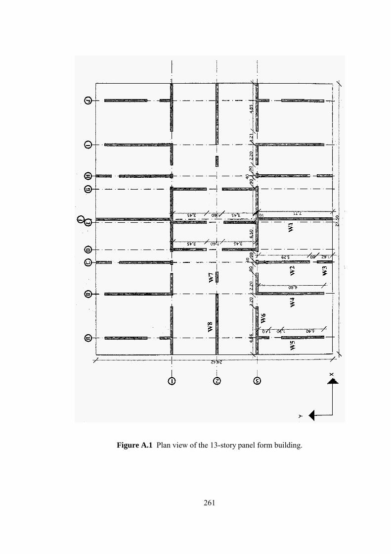
261
Figure A.1 Plan view of the 13-story panel form building.

262
A.2 INVESTIGATION OF THE 13-STORY PANEL BUILDING ALONG X
DIRECTION
Structural analysis and moment-curvature results of structural walls along X
direction are given in Table A.1. Figures A.2, A.3 and A.4 show the comparison of
moment curvature diagrams of W1, W6 and W8 when the earthquake action is along
the global X direction.
Table A.1 Structural analysis and moment-curvature results of structural walls along
X direction.
Wall
No
Structural
Analysis
Results
Minimum Amount of Mesh
Reinforcement
(ρsv,ρsh =0.0015)
End Zones at the boundaries of
the walls according to
(AY-1997)
W M(kNm) Mcr Mu Mu / Mcr Mcr Mu Mu / Mcr
1 170307 12835 12166 0.95 15490 35395 2.291
6 23204 2058 2016 0.979 2288 5675 2.48
8 42613 3759 4427 1.178 4075 8769 2.15

263
0
5000
10000
15000
20000
25000
30000
35000
40000
0 1 2 3 4 5 6 7 8 9 10 11 12 13 14 15
Curvature (rad/km)
Mom
ent (
kNm
)ρρρρ = 0.0015 and boundary reinforcement (AY-1997)
ρρρρ = 0.0015
Figure A.2 Comparison of moment curvature diagrams of W1 along X direction.
0
1000
2000
3000
4000
5000
6000
0 1 2 3 4 5 6 7 8 9 10 11
Curvature (rad/km)
Mom
ent (
kNm
)
ρρρρ = 0.0015
ρρρρ = 0.0015 and boundary reinforcement (AY-1997)
Figure A.3 Comparison of moment curvature diagrams of W6.

264
0
1000
2000
3000
4000
5000
6000
7000
8000
9000
10000
0 1 2 3 4 5 6 7 8 9 10
Curvature (rad/km)
Mom
ent (
kNm
)ρρρρ = 0.0015 and boundary reinforcement (AY-1997)
ρρρρ = 0.0015
Figure A.4 Comparison of moment curvature diagrams of W8.
A.3 INVESTIGATION OF THE 13-STORY PANEL BUILDING ALONG Y
DIRECTION
Structural analysis and moment-curvature results of structural walls along Y
direction are given in Table A.2. Figures A.5 and A.6 show the comparison of
moment curvature diagrams of W1 when the earthquake action is along Y and –Y of
the cross section, respectively. In Table A.2 it is named as 1Y and –1Y when the
earthquake action is along Y and –Y of the cross section, respectively. Figures A.7,
and A.8 show the comparison of moment curvature diagrams of W2 and W3 along Y
direction, respectively. Moment curvature diagram of SW4 is drawn for the flange,
which is in tension and compression. In Table A.2 it is named as SW4T and SW4C
when the flange of SW4 is in tension and compression, respectively. Figures A.9 and
A.10 show the comparison of moment curvature diagrams of SW4 when the flange is
in tension and compression, respectively. Comparison of moment curvature diagrams
of W5 is shown in Figure A.11.
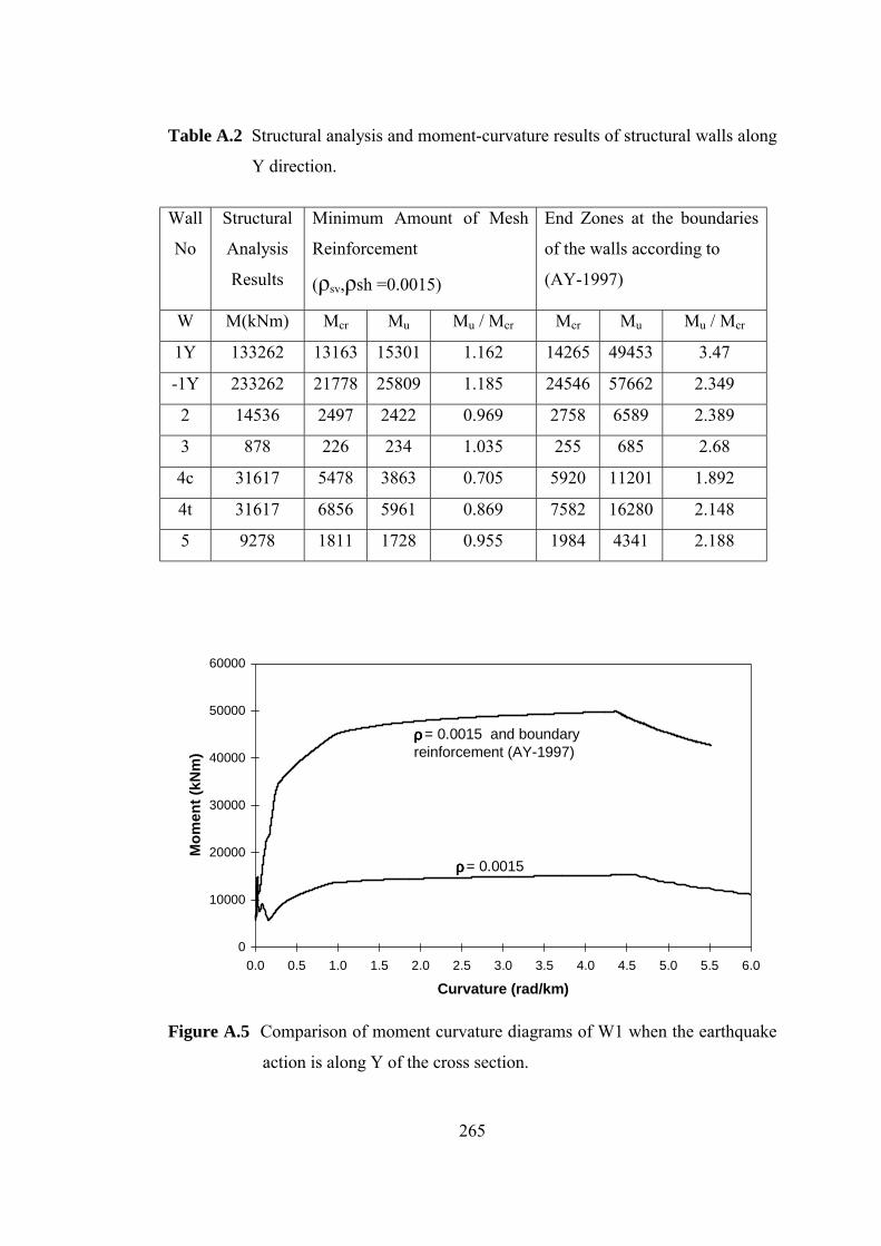
265
Table A.2 Structural analysis and moment-curvature results of structural walls along
Y direction.
Wall
No
Structural
Analysis
Results
Minimum Amount of Mesh
Reinforcement
(ρsv,ρsh =0.0015)
End Zones at the boundaries
of the walls according to
(AY-1997)
W M(kNm) Mcr Mu Mu / Mcr Mcr Mu Mu / Mcr
1Y 133262 13163 15301 1.162 14265 49453 3.47
-1Y 233262 21778 25809 1.185 24546 57662 2.349
2 14536 2497 2422 0.969 2758 6589 2.389
3 878 226 234 1.035 255 685 2.68
4c 31617 5478 3863 0.705 5920 11201 1.892
4t 31617 6856 5961 0.869 7582 16280 2.148
5 9278 1811 1728 0.955 1984 4341 2.188
0
10000
20000
30000
40000
50000
60000
0.0 0.5 1.0 1.5 2.0 2.5 3.0 3.5 4.0 4.5 5.0 5.5 6.0
Curvature (rad/km)
Mom
ent (
kNm
)
ρρρρ = 0.0015 and boundary reinforcement (AY-1997)
ρρρρ = 0.0015
Figure A.5 Comparison of moment curvature diagrams of W1 when the earthquake
action is along Y of the cross section.

266
0
10000
20000
30000
40000
50000
60000
70000
0.0 0.5 1.0 1.5 2.0 2.5 3.0 3.5 4.0
Curvature (rad/km)
Mom
ent (
kNm
)ρρρρ = 0.0015 and boundary reinforcement (AY-1997)
ρρρρ = 0.0015
Figure A.6 Comparison of moment curvature diagrams of W1 when the earthquake
action is along -Y of the cross section dimension.
0
1000
2000
3000
4000
5000
6000
7000
0 1 2 3 4 5 6 7 8 9 10 11
Curvature (rad/km)
Mom
ent (
kNm
)
ρρρρ = 0.0015
ρρρρ = 0.0015 and boundary reinforcement (AY-1997)
Figure A.7 Comparison of moment curvature diagrams of W2.

267
0
100
200
300
400
500
600
700
800
0 2 4 6 8 10 12 14 16 18 20 22 24 26 28 30 32
Curvature (rad/km)
Mom
ent (
kNm
)ρρρρ = 0.0015 and boundary reinforcement (AY-1997)
ρρρρ = 0.0015
Figure A.8 Comparison of moment curvature diagrams of W3.
0
2000
4000
6000
8000
10000
12000
14000
16000
18000
0 1 2 3 4 5 6 7
Curvature (rad/km)
Mom
ent (
kNm
)
ρρρρ = 0.0015 and boundary reinforcement (AY-1997)
ρρρρ = 0.0015
Figure A.9 Comparison of moment curvature diagram of W4 when the flange is in
tension.

268
0
2000
4000
6000
8000
10000
12000
14000
0 1 2 3 4 5 6 7 8 9 10 11 12
Curvature (rad/km)
Mom
ent (
kNm
)ρρρρ = 0.0015 and boundary reinforcement (AY-1997)
ρρρρ = 0.0015
Figure A.10 Comparison of moment curvature diagrams of W4 when the flange is
in compression.
Figure A.11 Comparison of moment curvature diagrams of W5.
0
500
1000
1500
2000
2500
3000
3500
4000
4500
5000
0 1 2 3 4 5 6 7 8 9 10 11 12 13
Curvature (rad/km)
Mom
ent (
kNm
)
ρρρρ = 0.0015
ρρρρ = 0.0015 and boundary reinforcement (AY-1997)

269
Moment curvature diagrams of structural walls were drawn for minimum
amount of mesh reinforcement and also for end zones, which were provided at the
boundaries of the structural walls according to the Turkish Earthquake Code
(AY-1997). When the minimum amount of mesh reinforcement was used, the ratio
of the ultimate moment to the cracking moment (Mu / Mcr) is less than 1.25 for all
structural walls. When the end zones were provided at the boundaries of the
structural walls according to the Turkish Earthquake Code (AY-1997), the ratio of
the ultimate moment to the cracking moment (Mu / Mcr) is greater than 1.25 for all
structural walls. It is obvious that when end reinforcement is placed at the boundaries
of the structural walls, brittle failure does not occur. It is clear from the Tables A.1
and A.2 the moments which is developed due to load combination of 1G + 1Q + 1E
are greater than the ultimate and cracking moments of the shearwalls.

270
APPENDIX B
EARTHQUAKE FORCES ON THE MODELS AND
PROTOTYPES
B.1 INTRODUCTION
In this part of the study 1/5-scale panel form test specimens are called models
and real size i.e. 1/1-scale panel form specimens are called prototypes. Equivalent
lateral earthquake forces on the 1/5-scale panel form test specimens are calculated
and compared with the applied lateral loads in the static tests. Also equivalent lateral
forces and overturning moments on the 1/1 real size panel form specimens
(prototype) are calculated and compared with the maximum load and moment
carrying capacity.
Dead weight of concrete is assumed to be 25 kN/m3, and 2.5 kN/m2 of live
load is uniformly distributed along the slab. Additional dead and live load is also
considered which is coming from the tributary area. Characteristic cylindrical
strength of concrete is 35 MPa. Models and prototypes are assumed to be located in
Seismic Zone-I in Turkey, so an effective ground acceleration coefficient (Ao) of
0.4g. Load reduction factor (R) is taken as one. Spectrum characteristic periods TA
and TB have the values of 0.10 and 0.3 seconds, respectively, by assuming soil class
as Z1.
B.2 EQUIVALENT LATERAL FORCES ON THE MODELS
In the static test of the models SP1 and SP2 maximum applied lateral loads
were 40 kN and 80 kN, respectively. Equivalent lateral force procedure is applied

271
and total design base shear of the 1/5-scale panel form test specimens (models) SP1
and SP2 are calculated as follows. The weight of the 1/5-scale panel form test
specimens is 50 kN including additional dead weight from the tributary area and live
load. Earthquake load reduction coefficient Ra(T) is taken as one.
Total Design Base Shear of the 1/5 scale panel form test specimen (model) SP1
kN40FkN31)T(R/)T(WAV erimentalexp1a1t =<== (B.1)
Total Design Base Shear of the 1/5 scale panel form test specimen (model) SP2
kN80FkN27)T(R/)T(WAV erimentalexp1a1t =<== (B.2)
It is understood from Equations B.1 and B.2 that total design base shears due
to earthquake of the 1/5-scale panel form test specimens are smaller than the applied
lateral load in the static tests (Fexperimental).
Total Design Base Shear due to earthquake of the 1/5 scale panel form test
specimen (model) does not represent the actual case. To determine actual earthquake
loads 1/1 scale prototype models will be considered.
The ratio of the moment of inertia of the prototype to the moment of inertia of
the model ( Iprot / I model ) for SP1 and SP2 is 625. The ratio of the weight of the
prototype to the weight of the model ( Wprot / Wmodel ) for SP1 and SP2 is 125.
The ratio of the moment of inertia of the prototype to that of the model is 625
for both SP1 and SP2, however the ratio of the weight of the prototype to the weight
of the model is 125 for SP1 and SP2. Since the ratio of the moment of inertias and
the ratios of weights (mass) for the prototype to model are not equal, it is not
appropriate to compare the equivalent lateral earthquake force and lateral force
applied in the static test by using the model. Therefore, the prototype will be used to
calculate the equivalent earthquake forces. From the equivalent earthquake forces the
moment at the base will be calculated and compared with the moment carrying
capacity of the sections.
In the prototypes cross section two-layer minimum amount of mesh
reinforcement is used. Spacing of the longitudinal mesh reinforcement is 150 mm.

272
To provide 0.15% mesh reinforcement ratio in the vertical and longitudinal
directions along the wall depth, 5.5 mm diameter two-layer mesh reinforcement was
used.
Figures B.1 and B2 show the moment curvature diagram of 1/1 scale
(prototype) SP1 and SP2, respectively. For the prototype SP1 and SP2 the ratio of
ultimate moment to cracking moment is 0.597 and 1.12, respectively. Moment due to
earthquake is 41158 kNm for both SP1 and SP2, respectively. It is understood from
Figures B1 and B2 that moment due to earthquake is greater than the moment
carrying capacity of the prototype panel form specimens SP1 and SP2.
0
5000
10000
15000
20000
25000
30000
35000
40000
45000
0 1 2 3 4 5 6 7 8 9
Curvature (rad/km)
Mom
ent (
kNm
)
Moment due to earthquake
Figure B.1 Moment curvature diagram of 1/1 scale (prototype) SP1.

273
0
5000
10000
15000
20000
25000
30000
35000
40000
45000
0 0.5 1 1.5 2 2.5 3 3.5 4 4.5 5
Curvature (rad/km)
Mom
ent (
kNm
)Moment due to earthquake
Figure B.2 Moment curvature diagram of 1/1 scale (prototype) SP2.
274
VITA
S. Bahadır YÜKSEL was born in Ankara on November 24, 1971. He received
his B.Sc. degree from Selçuk University in 1994 and M.Sc. degree from Middle East
Technical University in 1997. His main area of interest is panel form structures.
EDUCATION
September 1997- present : Middle East Technical University, Ankara, Turkey
Civil Engineering, PhD, GPA: 3.84/4.00
February 1994- June 1997 : Middle East Technical University, Ankara, Turkey
Civil Engineering, Master of Science GPA: 3.84/4.00
September 1989- June 1993 : Selçuk University, Konya, Turkey Civil Engineering,
Bachelor of Science GPA: 82.00/100
EXPERIENCE
October 1994-March 2003 RESEARCH ASSISTANT(involves teaching).
Department of Civil Engineering, Division of Structural Mechanics, Middle East
Technical University, Turkey. Have been responsible for the following courses
(teaching assist): CE384 Structural Analysis, CE382-Reinforced Concrete
Fundamentals, CE483 Advanced Structural Analysis, CE481-Reinforced Concrete
Structures, CE222-Engineering Mechanics II.

275
COMPUTER SKILLS
• Use of Finite Element program SAP, nonlinear inelastic dynamic analysis
program DRAIN.
• Development of softwares using BASIC, FORTRAN.
• Several editing, graphical and spreadsheet programs.
• MS-DOS and Windows-2000 Operating Systems.
• Many Internet Applications.
LANGUAGES
English
LIST OF PUBLICATIONS
Yüksel, B., Atımtay, E., (2001) “Tünel Kalıplı Yüksek Binaların Deprem Davranışı
ve Güvenliği”.Yapı Mekaniği Laboratuvarları Toplantısı Bildiriler ve Laboratuvar
Olanakları, 5-6 Kasım 2001, Ankara pp. 97-104.
Yüksel, B., Atımtay, E., (2003) “Tünel Kalıplı Yüksek Binaların Yatay Yük Altında
Davranışı ”.Yapı Mekaniği Laboratuvarları Toplantısı II, 19-20 Haziran 2003, Konya
pp. 21-26.
Yüksel, B., (1997) “A Comparative Study on Seismic Codes ” Master Thesis in Civil
Engineering, Middle East Technical University, September 1997.
HONORS
Award for being best undergraduate study in Selçuk University (1994).