1

Experimental Investigation of Frequency DomainChannel Extrapolation in Massive MIMO Systems

for Zero-Feedback FDDThomas Choi, Student Member, IEEE, François Rottenberg, Member, IEEE,

Jorge Gomez-Ponce, Student Member, IEEE, Akshay Ramesh, Student Member, IEEE,Peng Luo, Student Member, IEEE, Jianzhong Zhang, Fellow, IEEE, and Andreas F. Molisch, Fellow, IEEE

Abstract—Estimating downlink (DL) channel state information(CSI) in frequency division duplex (FDD) massive multi-inputmulti-output (MIMO) systems generally requires downlink pilotsand feedback overheads. Accordingly, this paper investigates thefeasibility of zero-feedback FDD massive MIMO systems basedon channel extrapolation. We use the high-resolution parameterestimation (HRPE), specifically the space-alternating generalizedexpectation-maximization (SAGE) algorithm, to extrapolate theDL CSI based on the extracted parameters of multipath com-ponents in the uplink channel. We apply the HRPE to twodifferent channel models: the vector spatial signature (VSS)model and the direction of arrival (DOA) model. We verify thesemethods through real-world channel data acquired from channelmeasurement campaigns with two different types of channelsounders: a) a switched array-based, real-time, time-domain,outdoors setup at 3.5 GHz, and b) a virtual array-based, high-accuracy, frequency-domain, indoors setup at 2.4 and 5−7 GHz.The performance metrics of the extrapolated channels that weevaluate include the mean squared error, beamforming efficiency,and spectral efficiency in multiuser MIMO scenarios. The resultsshow that the HRPE-based channel extrapolation performs bestunder the simple VSS model, which does not require arraycalibration, and if the BS is in an open outdoor environmenthaving line-of-sight (LOS) paths to well-separated users.

Index Terms—Zero-feedback FDD massive MIMO, channelextrapolation, SAGE, vector spatial signature (VSS), channelmeasurement, channel sounder, multiuser MIMO.

I. INTRODUCTION

A. Motivation and Problem Statement

MAssive multi-input multi-output (MIMO) systems uti-lize tens to hundreds of antennas at the base station

(BS) to increase the spectral and energy efficiency of wirelessnetworks [2]–[4]. This makes them a promising solution to therapidly growing number of wireless devices and soaring data

The work was supported by the National Science Foundation (ECCS-1731694), the Belgian National Science Foundation (FRS-FNRS), the BelgianAmerican Educational Foundation (BAEF), the Foreign Fulbright EcuadorSENESCYT Program, and Samsung Research America. A part of this articlewas presented at the VTC2019-Fall [1].

T. Choi, J. Gomez-Ponce, A. Ramesh, P. Luo, and A. F. Molisch are with theMing Hsieh Department of Electrical and Computer Engineering, Universityof Southern California, Los Angeles, CA, USA. J. Gomez-Ponce is also withthe ESPOL Polytechnic University, Escuela Superior PolitÃl’cnica del Litoral,ESPOL, Facultad de Ingeniería en Electricidad y Computación, Km 30.5 và aPerimetral, P. O. Box 09-01-5863, Guayaquil, Ecuador. F. Rottenberg is withthe UniversitÃl’ catholique de Louvain, Louvain-la-Neuve, Belgium and theUniversitÃl’ libre de Bruxelles, Brussels, Belgium. J. Zhang is with SamsungResearch America, Richardson, TX, USA. Corresponding author: ThomasChoi (choit@usc.edu).

capacity requirements. Massive MIMO systems are generallyassumed to operate in time division duplex (TDD) mode,where both the uplink (UL) and the downlink (DL) share thesame frequency band [4]–[6].1 In TDD mode, the massiveMIMO system exploits the channel reciprocity, attaining theDL channel state information (CSI) from UL pilots.2

In comparison, the UL and the DL bands are separatedin the frequency division duplex (FDD) mode. Because thechannel coherence bandwidth (BW) is almost always muchsmaller than the duplex spacing [10], the channel reciprocitycannot be directly exploited. Therefore, extra overheads, suchas DL pilots and feedback, are necessary to attain DL CSI.Also, these overheads scale with the number of antennas at theBS rather than with the total number of antennas at the userequipments (UEs), which may become prohibitive as massiveMIMO systems usually have a large number of BS antennas.

Although such high resource demands from the FDD mas-sive MIMO suggest employing the optimal TDD operationfor massive MIMO systems, many legacy wireless networksstill operate in the FDD frequency spectrum [10]. Therefore,FDD massive MIMO systems can reduce costs which mayarise from modifying the hardware, frequency allocations,and network operation when upgrading the legacy BSs intomassive MIMO BSs. One possible solution to enable FDDmassive MIMO based on the UL pilots only (like the TDDmassive MIMO) is through channel extrapolation (see sec. I-Cfor the literature review).

In [11], [12], we theoretically investigated an approach inwhich the channel extrapolation uses high-resolution parame-ter estimation (HRPE). The HRPE determines the parametersof each multipath component (MPC) (e.g., complex amplitude,delay, azimuth direction of arrival (DOA), elevation DOA, etc.)in the UL channel (also known as the training band in thechannel extrapolation context) based on the UL pilots. Thetransfer function of a wireless channel is the complex sum ofthe contributions of the individual MPCs; thus, the BS canestimate the channel in the DL band without any DL pilotsor feedback, assuming that the MPC parameters in the DLchannel are the same as those in the UL channel (see Fig. 1).

1In fact, several researchers have defined that massive MIMO systemsoperate in TDD mode by default [4].

2The reciprocity assumption holds only when the transceivers are calibrated[7]–[9] and when both the UL and the DL occur within the channel coherencetime—usually in scales of milliseconds.

arX

iv:2

003.

1099

1v2

[ee

ss.S

P] 2

9 Se

p 20

20

2

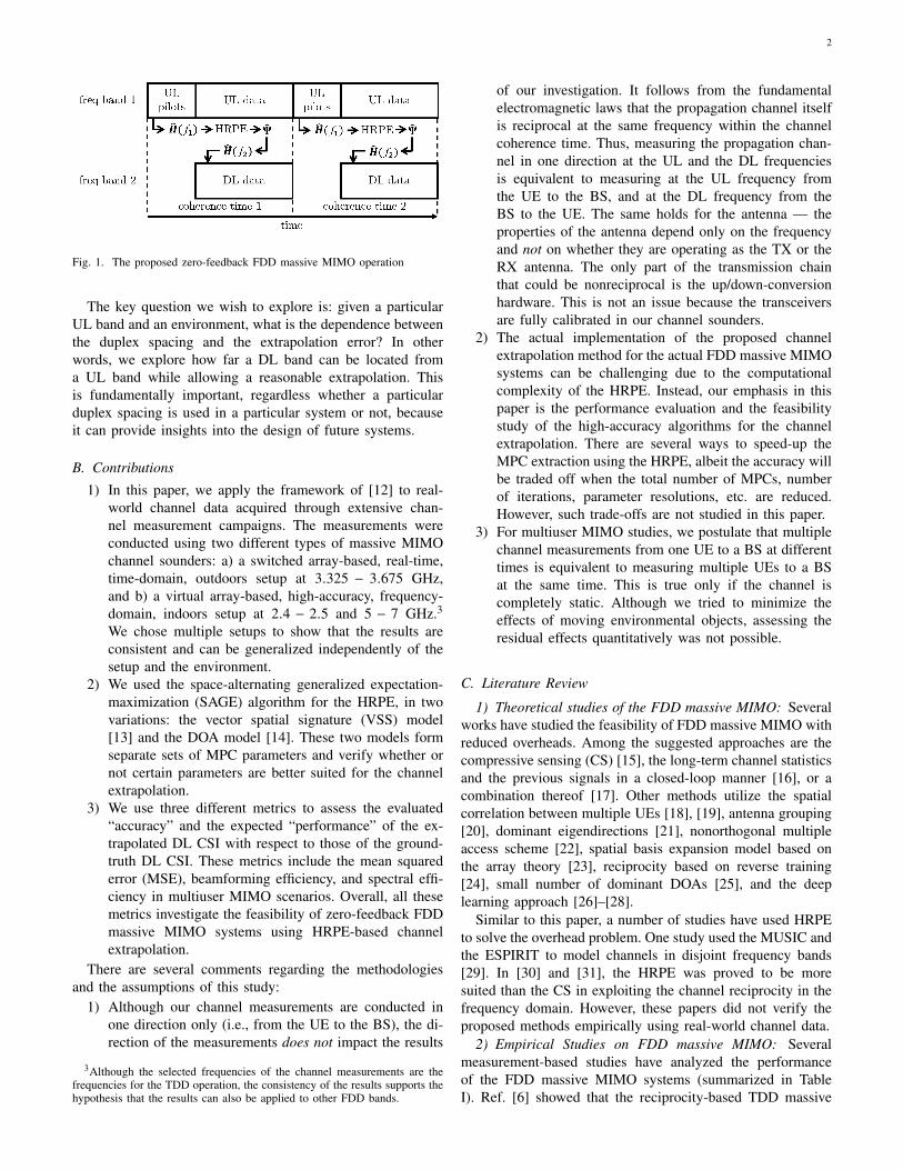
Fig. 1. The proposed zero-feedback FDD massive MIMO operation

The key question we wish to explore is: given a particularUL band and an environment, what is the dependence betweenthe duplex spacing and the extrapolation error? In otherwords, we explore how far a DL band can be located froma UL band while allowing a reasonable extrapolation. Thisis fundamentally important, regardless whether a particularduplex spacing is used in a particular system or not, becauseit can provide insights into the design of future systems.

B. Contributions

1) In this paper, we apply the framework of [12] to real-world channel data acquired through extensive chan-nel measurement campaigns. The measurements wereconducted using two different types of massive MIMOchannel sounders: a) a switched array-based, real-time,time-domain, outdoors setup at 3.325 − 3.675 GHz,and b) a virtual array-based, high-accuracy, frequency-domain, indoors setup at 2.4 − 2.5 and 5 − 7 GHz.3

We chose multiple setups to show that the results areconsistent and can be generalized independently of thesetup and the environment.

2) We used the space-alternating generalized expectation-maximization (SAGE) algorithm for the HRPE, in twovariations: the vector spatial signature (VSS) model[13] and the DOA model [14]. These two models formseparate sets of MPC parameters and verify whether ornot certain parameters are better suited for the channelextrapolation.

3) We use three different metrics to assess the evaluated“accuracy” and the expected “performance” of the ex-trapolated DL CSI with respect to those of the ground-truth DL CSI. These metrics include the mean squarederror (MSE), beamforming efficiency, and spectral effi-ciency in multiuser MIMO scenarios. Overall, all thesemetrics investigate the feasibility of zero-feedback FDDmassive MIMO systems using HRPE-based channelextrapolation.

There are several comments regarding the methodologiesand the assumptions of this study:

1) Although our channel measurements are conducted inone direction only (i.e., from the UE to the BS), the di-rection of the measurements does not impact the results

3Although the selected frequencies of the channel measurements are thefrequencies for the TDD operation, the consistency of the results supports thehypothesis that the results can also be applied to other FDD bands.

of our investigation. It follows from the fundamentalelectromagnetic laws that the propagation channel itselfis reciprocal at the same frequency within the channelcoherence time. Thus, measuring the propagation chan-nel in one direction at the UL and the DL frequenciesis equivalent to measuring at the UL frequency fromthe UE to the BS, and at the DL frequency from theBS to the UE. The same holds for the antenna — theproperties of the antenna depend only on the frequencyand not on whether they are operating as the TX or theRX antenna. The only part of the transmission chainthat could be nonreciprocal is the up/down-conversionhardware. This is not an issue because the transceiversare fully calibrated in our channel sounders.

2) The actual implementation of the proposed channelextrapolation method for the actual FDD massive MIMOsystems can be challenging due to the computationalcomplexity of the HRPE. Instead, our emphasis in thispaper is the performance evaluation and the feasibilitystudy of the high-accuracy algorithms for the channelextrapolation. There are several ways to speed-up theMPC extraction using the HRPE, albeit the accuracy willbe traded off when the total number of MPCs, numberof iterations, parameter resolutions, etc. are reduced.However, such trade-offs are not studied in this paper.

3) For multiuser MIMO studies, we postulate that multiplechannel measurements from one UE to a BS at differenttimes is equivalent to measuring multiple UEs to a BSat the same time. This is true only if the channel iscompletely static. Although we tried to minimize theeffects of moving environmental objects, assessing theresidual effects quantitatively was not possible.

C. Literature Review

1) Theoretical studies of the FDD massive MIMO: Severalworks have studied the feasibility of FDD massive MIMO withreduced overheads. Among the suggested approaches are thecompressive sensing (CS) [15], the long-term channel statisticsand the previous signals in a closed-loop manner [16], or acombination thereof [17]. Other methods utilize the spatialcorrelation between multiple UEs [18], [19], antenna grouping[20], dominant eigendirections [21], nonorthogonal multipleaccess scheme [22], spatial basis expansion model based onthe array theory [23], reciprocity based on reverse training[24], small number of dominant DOAs [25], and the deeplearning approach [26]–[28].

Similar to this paper, a number of studies have used HRPEto solve the overhead problem. One study used the MUSIC andthe ESPIRIT to model channels in disjoint frequency bands[29]. In [30] and [31], the HRPE was proved to be moresuited than the CS in exploiting the channel reciprocity in thefrequency domain. However, these papers did not verify theproposed methods empirically using real-world channel data.

2) Empirical Studies on FDD massive MIMO: Severalmeasurement-based studies have analyzed the performanceof the FDD massive MIMO systems (summarized in TableI). Ref. [6] showed that the reciprocity-based TDD massive

3

TABLE ILIST OF EMPIRICAL FDD MASSIVE MIMO RESEARCH

Institution DL CSI selection/estimation method Feedback

Lund [6] the best beam among a grid of beams yes

Rice [32] maximum likelihood method [37] for thedominant DOAs yes

Ericsson [33] modified maximum likelihood method [38] noMIT [34] R2-F2 [34] no

Stuttgart [35] deep learning noUSC SAGE VSS [13] / DOA [14] no

MIMO performs better than the feedback-based FDD massiveMIMO with predetermined grid of beams, especially in thenon-line-of-sight (NLOS) cases, based on channel measure-ments at 2.6 GHz carrier frequency and 50 MHz measurementbandwidth. In [32], the authors used the DL training andthe feedback only toward the four dominant DOAs in orderto reduce the overheads. The results showed that spectralefficiency improved by 150 percent compared to that of the fulltraining and the feedback. Channel measurements were thenconducted using 64 antennas at 2.4 GHz carrier frequency, 20MHz training band, and 72 MHz duplex spacing.

Several papers experimentally investigated the “zero feed-back methods” for FDD massive MIMO. Ref. [33] used 8× 8MIMO measurements and a modified maximum likelihoodestimator to investigate the extrapolation performance in thespatial and the frequency domains using 5 MHz trainingband within 2.4–2.45 GHz. Ref. [34] employed the “R2-F2”method, which utilizes the phase changes from inter-antennaseparation at the BS to estimate the channel at another fre-quency band. The proposed FDD system with the extrapolatedchannel showed high beamforming efficiency. However, onlyfive antennas were used at the BS, with 10 MHz trainingband within 640–690 MHz. Another zero-feedback methodrelied on deep learning, which uses a large amount of trainingdata to predict the DL CSI based on the UL CSI [35]. Themeasurement setup used 32 antennas at the BS, with 20 MHztraining band and 25 MHz duplex spacing within 1.2–1.3 GHz.

The current paper differs from other papers and expands ourprevious results [1], [11], [12] by: 1) using another channelmodel (VSS) that has the advantage of not requiring anarray pattern calibration in the HRPE evaluation and channelextrapolation, 2) using an additional channel sounder (virtualarray-based, high-accuracy, frequency-domain, indoors setups,at 2.4−2.5 and at 5−7 GHz) to verify consistency of the resultsin different settings, and 3) employing an additional figureof merit (the spectral efficiency) in the multiuser massiveMIMO systems. More recently, [36] used a similar channelinference method using the SAGE and four other differenttypes of calibration methods. However, only a DOA model thatexcludes the elevation DOA was used in the paper. Moreover,the measurement BW was smaller, at less locations, and themultiuser scenarios were not considered.

II. VSS AND DOA CHANNEL MODELS

In this work, we 1) estimate the MPC parameters usingan HRPE based on the parametric channel models, and

subsequently get complete descriptions of the channels atthe training (UL) band (an arbitrarily selected subset of themeasured frequency band); and 2) extrapolate the estimatedCSI to the other (DL) frequency band (the complement band ofthe training band within the measured frequency band) usingthe parameters obtained from the training band. The overallinputs and outputs of the HRPEs depending on two differentparametric channel models are shown in Fig. 2. These will beexplained in the succeeding subsections.

A. Channel Matrix for the HRPE

First, we select a raw channel matrix measured by thereceiver of a channel sounder, Hmeas, with dimension M×K . Mis the number of antennas at the BS, whereas K is the numberof frequency samples of the measurement. The subscript measindicates that the data have not yet been compensated for theresponse of the calibrated radio frequency (RF) system, hRF.hRF = [hRF,1, hRF,2, . . . , hRF,K]T is a K × 1 vector of scalars,which is the back-to-back calibration response of the soundertransmitter (TX) and the receiver (RX) connected by a cable(excluding the antennas and the channel).4 The compensatedfrequency response of the channel and the antennas only, H ,is attained by

H = Hmeas ·

(hRF,1)−1 0 · · · 0

0 (hRF,2)−1 · · · 0...

.... . .

...

0 0 · · · (hRF,K)−1

. (1)

We define averaged power of H as µH2 =

| |H | |2FMK , where

| | · | |F is the Frobenius norm, and the normalized channelmeasurement matrix as H = H

µH. If Ku ≤ K is the number

of frequency points in the arbitrarily selected training bandwithin the measurement band, an M × Ku subset of H ,Hu = H(:, a:a+Ku−1) with 1 ≤ a ≤ K − Ku + 1, represents themeasured channel matrix at the training band. Hu becomes theinput for the HRPE.

Although there are many well-known HRPEs (e.g., MUSIC[39], ESPRIT [40], CLEAN [41], and RiMAX [42]), weselected the SAGE algorithm arbitrarily, as the extrapolationresults during the preliminary analysis were dependent onthe channel models rather than on the type of HRPEs. Twochannel models (i.e., the VSS and the DOA) are used to attainthe different types and values of the MPC parameters. Thiswill be further discussed in the succeeding subsections. Amore detailed description of the SAGE algorithm is given inAppendix A.

B. Vector Spatial Signature (VSS) Model

The main difference between the VSS and the DOA modelsis that the former does not require a calibrated array pattern,

4hRF is a 1-D frequency response because each of the switched and thevirtual array setups we used relies on a single RF chain for all antennas—it canbe a matrix for other setups if multiple RF chains are used. This notation mustnot be confused with the impulse response notation, which usually employslower case letter.

4

Fig. 2. A detailed process of the channel extrapolation using the SAGE algorithm based on the VSS and the DOA models

A, as it does not estimate the DOAs of MPCs. The onlyinput for the VSS algorithm, other than the normalized channelmeasurement matrix at the UL band, Hu, is L, which is thenumber of MPCs (Fig. 2). In terms of channel extrapolation,describing the channel with large L may result in lower pre-diction accuracy due to overfitting. Furthermore, MPCs withlower amplitudes will be more prone to noise, and thus maydeteriorate the overall channel prediction in the extrapolatedband. Therefore, the selected L needs to be sufficiently largeto estimate the training band accurately (MSE < −10 dB),but small enough to prevent overfitting. This compromise wasfound empirically, and the choice of L accordingly differedbetween measurements under different environments [1].

The first parameter of the VSS model is the estimated delay,τv , where v is the index of the MPC. The second parameteris called the “vector spatial signature (VSS)”, represented byav . av is a frequency independent complex vector with sizeM×1. According to [13], the VSSs are “not explicit functionsof DOA, but instead abstractly represent the response of the

array pattern for the path v with the delay τv”.The extrapolation range is limited in the VSS model be-

cause in practice, most array patterns are frequency-dependent.However, estimating within the training band will be veryaccurate for massive MIMO systems because the number ofthe estimated parameters in the VSS model scales with M;these parameters can then be adjusted to best estimate thechannel response.

The VSS channel model is overall expressed as:

HVSS( f ) =L∑

v=1ave−j2π f τv . (2)

Once both av and τv are estimated for all L paths from thetraining band, the CSI at the desired frequency (such as theDL frequency in the FDD systems), fd, can be attained bysetting f = fd in eq. (2). The VSS model hence assumes thatonly the phase changes with frequency.

In total, the VSS model estimates the 2ML + L real-valuedparameters, where the first term 2ML is the total number

5

TABLE IIESTIMATED MPC PARAMETERS IN THE VSS AND THE DOA CHANNEL MODELS

Model Estimated MPC parameters Channel modelVSS ψv = [av, τv ] HVSS ( f ) =

∑Lv=1 ave

− j2π f τv

DOA ψd = [αd, τd, φd, θd ] HDOA( f ) =∑L

d=1 αdA(φd, θd, f )e− j2π f τd

of real and the imaginary values (2) of the vector spatialsignatures for all antennas (M) over all paths (L), and thesecond term L is the total number of delays.

C. Direction of Arrival (DOA) Model

As the name indicates, the DOA model requires a frequencydependent calibrated antenna array pattern, A, to determinethe DOAs of the incoming MPCs. Aside from the topic ofchannel extrapolation, this model is useful when the angularinformation of the channel is needed. Like the VSS model,the DOA model also requires the normalized channel mea-surement matrix in the UL band, Hu, and the total number ofMPCs, L (Fig. 2).

A is attained differently for switched array and virtual array[1]. In a switched array, a reference antenna with a knownpattern is positioned on one side of the anechoic chamber,and the switched array is positioned on another side thatis supported by a rotating positioner. The array rotates toa certain azimuth and elevation position, and then switcheson a selected antenna element. A vector network analyzer(VNA) then sweeps across the frequency to record the channelfrequency response. Subsequently, the next antenna element isturned on for another VNA sweep. After obtaining the transferfunction for each antenna element, the antenna array rotates toa new azimuth and elevation position; the process repeats torecord the channel frequency response at the selected position.

In the end, a 4-D calibration data, with dimension Naz×Nel×M×K , is created. Naz and Nel are the number of azimuth stepsand number of elevation steps during calibration, respectively.The calibrated array pattern at the training band, Au, is selectedas an input for the HRPE, with dimension Naz ×Nel ×M ×Ku.The complement set of Au within A will be used when thechannel is extrapolated to the frequency outside the trainingband.

The virtual array calibration, however, does not rely onswitching; thus, a calibration data of a single antenna withdimension Naz × Nel × K is created first. This 3-D calibrationdata of a single antenna is numerically rotated or moved Mtimes to form a 4-D calibration data of a virtual antennaarray with the selected geometry and numbers. The impactof the rotation/movement is computed geometrically, and notmeasured explicitly. The formulated calibration data, A, withdimension Naz × Nel × M × K , are then used in the same wayas the switched-array calibration data.

We have shown in [1] the output parameters of the MPCsattained through the SAGE algorithm based on the DOA modeland channel extrapolation results in an anechoic chamber andoutdoors. The estimated parameters of each MPC in the DOAmodel include the complex amplitude, α, delay, τ, azimuthDOA, φ, and elevation DOA, θ. In this paper, the subscript dis added to the parameters (αd , τd , φd , and θd) as an index of

the MPC in order to distinguish between the parameters of theVSS and the DOA models. These parameters are summarizedin Table II. There are 5L real-valued parameters (the real andthe imaginary values of the complex amplitude and other threeparameters per path over all paths) to estimate, which areusually much less than 2ML+L parameters in the VSS model.

The estimated parameters from the training band are putback into the channel model such that the channel frequencyresponse can be estimated at a selected frequency, f . The DOAchannel model is as follows:

HDOA( f ) =L∑

d=1αdA(φd, θd, f )e−j2π f τd (3)

where A(φd, θd, f ) is the M × 1 1-D slice of the 4-D arrayresponse over M antenna elements (switched array) or posi-tions (virtual array). It is dependent on the estimated azimuthDOA from the training band, estimated elevation DOA fromthe training band, and frequency of choice. The array patternat a specific frequency is obtained, either through includingthe frequency point during calibration or through interpolationif the desired frequency is between two measured frequencypoints during the calibration. The DOA model assumes boththe array response and the phase changes with frequency.

III. PERFORMANCE METRICS

We select the following three types of performance metricsto assess the performance of the extrapolation: the MSE,beamforming efficiency, and spectral efficiency for multiuserscenarios.

A. Mean Squared Error (MSE)

The MSE averages the squared magnitude of the differencesbetween the normalized complex channel response of a mea-sured (ground-truth) channel and the estimated channel at theselected frequency over all antennas:

MSE( f ) ∆=| |H( f ) − H( f )| |22

M(4)

where H( f ) is either HDOA( f ) or HVSS( f ) with dimensionM × 1 and | | · | |2 is the Euclidean norm. If f lies within thetraining band, then the MSE will be a measure of the interpola-tion performance. In comparison, if f lies outside the trainingband, then the MSE will be a measure of the extrapolationperformance. While the MSE measures the absolute accuracyof the extrapolated channel, it neglects the ability of the UEsto compensate for a common phase and amplitude error. TheMSE will be represented on a dB scale.

6

B. Beamforming Efficiency

Massive MIMO array obtains a beamforming gain (BG)by combining constructive contributions of the many antennaelements within the array. One common way to optimize theBG (in a single-user case) is through the maximum-ratio com-bining (the matched filtering) based on the estimated channelresponse. The beamforming efficiency (BE) indicates how theBG with the estimated CSI compares with that based on themeasured (ground-truth) CSI. The BG with the measured CSI,the estimated CSI, and the uniform beamforming are expressedas follows:

BGmeas( f )∆= | |H( f )| |22 (5)

BGest ( f )∆=|H( f )†H( f )|2

| |H( f )| |22(6)

BGuni( f )∆=| |H( f )| |22

M(7)

where † is the conjugate transpose operator. Therefore, usingeq. (5) and (6), the BE is expressed as follows:

BE( f ) ∆= BGest ( f )BGmeas( f )

=|H( f )†H( f )|2

| |H( f )| |22 | |H( f )| |22. (8)

This value ranges from 0 to 1, with 1 indicating full efficiency.Similar to the case of the MSE, the BE will be representedon a dB scale.

C. Spectral Efficiency in Multiuser MIMO Systems

The earlier metrics are based on the single-user assumption.The spectral efficiency in every UE of a multiuser MIMOsystem can be determined by single-user measurements atmultiple locations. The spectral efficiency of the UE n atfrequency f is represented as:

C(n)( f ) = log2(1 + SINR(n)( f )) [bits/s/Hz] (9)

where SINR(n)( f ) is a signal-to-interference-plus-noise ratioat a given frequency and UE. The index of each UE, n, variesfrom 1 to N . The received signal by the nth UE at frequencyf during the DL phase is:

r (n)( f ) = H (n)( f )TG(n)( f )s(n)

+

N∑n′,n

H (n)( f )TG(n′)( f )s(n′) + w(n) (10)

where T is a transpose operator; r (n)( f ) is a complex valuereceived by the UE n at the selected frequency, f ; H (n)( f )is the ground-truth channel vector for the UE n at frequencyf from every antenna, with dimension M × 1; G(n)( f ) is thenormalized precoding vector of the UE n at frequency f fromevery antenna with dimension M×1; s(n) is a transmitted signalfrom the BS for the UE n;and w(n) is a noise received by theUE n.

The first term indicates the beamforming signal for the UEn, whereas the second term indicates the interference from

the signals intended for other UEs received by the UE n.Therefore, SINR(n)( f ) is expressed as:

SINR(n)( f ) =|H (n)( f )TG(n)( f )|2σs(n)

2∑Nn′,n |H (n)( f )TG(n

′)( f )|2σs(n′)2 + σw(n)

2

(11)where σs(n)

2 and σw(n)2 are the variances of the signal and the

noise, assumed to be the same for all N UEs (i.e., all UEs areexpected to experience the same transmit power from the BSand the same noise power).

The normalized precoding vector, G(n)( f ), can be createdas follows. First,

HMU ( f ) = [H (1)( f ), H (2)( f ), ..., H (N )( f )]

=

H(1)1 ( f ) H(2)1 ( f ) · · · H(N )1 ( f )H(1)2 ( f ) H(2)2 ( f ) · · · H(N )2 ( f )

......

. . ....

H(1)M ( f ) H(2)M ( f ) · · · H(N )M ( f )

(12)

where H(n)m ( f ) represents an estimated complex channel valuebetween the BS antenna m and the UE n at frequency f . Then,the precoding matrix for the N UEs can be determined in twoways: the maximum ratio (MR) and the zero-forcing (ZF):

GMR( f ) = HMU ( f )† (13)

GZF ( f ) = HMU ( f )†(HMU ( f )HMU ( f )†)−1. (14)

Dimension of both matrices is N×M . G(n)( f ) is a precodingvector of the UE n at frequency f with dimension M × 1 (thetranspose of row n of either GMR( f ) or GZF ( f )). Finally,we normalize this precoding vector to get the normalizedprecoding vector per UE, G(n)( f ) = G(n)( f )

| |G(n)( f ) | |2.

IV. MEASUREMENT SETUPS AND SETTINGS

We conducted the measurement campaigns using two typesof channel sounders under different environments. Each ofthese methods has respective advantages and drawbacks.The “time-domain” setup, which is based on the arbitrarywaveform generator (AWG) and the digitizer combined withthe fast-switching array, enables measurements under fast-varying environments. On the other hand, the âAIJfrequency-domainâAI setup, which is based on the vector network ana-lyzer (VNA) combined with a single antenna forming a virtualarray, enables high-precision measurements without antennacoupling or element impairments. The list of commercial off-the-shelf hardware used to build the sounders is given in TableIII.

In both channel sounders, an omnidirectional antenna isused at the TX that emulates a UE. On the RX (BS) side, theswitched array is used during the outdoor measurements andthe rotating horn during the indoor measurements. In order toconsider the measured channel as the reference “ground-truth”channel such that the estimated channel can be comparedwith, a high signal-to-noise ratio (SNR) was necessary duringthe measurement. Therefore, we used an effective isotropicradiated power (EIRP) up to 40 dBm during the outdoor

7

TABLE IIILIST OF CHANNEL SOUNDER EQUIPMENT

Type Real-time sounder with switched array VNA-based sounder with rotating hornTransmitter Agilent N8241A AWG Keysight E5080A VNA

Receiver NI PXIe-5160 Oscilloscope Keysight E5080A VNAClock Precision Test Systems GPS10eR internal clock within VNAMixer Mini-Circuits ZEM-4300MH+ N/A

Local Oscillator Phase Matrix FSW-0020 N/A

Amplifier

Mini-Circuits ZFL-500LNMini-Circuits ZHL-100W-382+

Wenteq ABP1500-03-3730Wenteq ABL0600-33-4009

Wenteq ABP1500-03-3730Wenteq ABL0800-12-3315

Filters Pasternack PE8713Mini-Circuits ZBP-2450+Mini-Circuits VHF3800Mini-Circuits VLF7200+

Antennas Lab-built stacked patch arrayCobham XPO2V-0.3-10.0/1381

L-com HG2420EG-NFA-INFO LB-159-20-C-SF

Cobham XPO2V-0.3-10.0/1381

Switch Pulsar SW8ADPulsar SW16AD N/A

Positioner N/A Dams DCP252A

measurements and another EIRP up to 28 dBm during theindoor measurements.

Because the outdoor measurements were conducted withoutany vehicular movements, the changes in the environment oc-curred only from walking pedestrians and moving vegetation.Even with a 10 km/h maximum speed assumption, the coher-ence time is in the order of 30 ms at 3.5 GHz frequency. Theswitched array-based, time-domain channel sounder capturesthe channel responses between the UE antenna and all the BSantennas in 10.24 ms, which is well within the outdoor chan-nel coherence time. In the indoor measurement, meanwhile,although the virtual array-based, frequency-domain channelsounder takes several minutes to capture the channel, weconducted the measurements late at night when there wereno people. This then ensured that there was no movement inthe environment, leading to (theoretically) infinite coherencetime.

A. Outdoor Measurements with Switched Array

To measure the channel characteristics of the outdoor chan-nels with short coherence time, we used a switched array with64 antenna elements as the RX, thereby emulating a massiveMIMO BS (Fig. 3a). The antenna array is cylindrical and has16 columns of 6 × 1 linear antenna array. Each antenna hasa stacked patch design, which increases the beamwidth andthe BW as compared to the conventional patch antennas. Fourantenna elements per column are used during the measurementsince we use the top and bottom antenna elements (per eachcolumn) as the “dummy” antenna elements. This then resultsin 64 active antenna elements. Although each antenna elementhas two ports (vertical/horizontal polarization) , we consideronly the vertically polarized ports because the TX uses avertically polarized antenna. The radiation patterns of theantenna elements are also described in [1].

These 64 active antenna elements are then connected toeight 16×1 switches. The switches are cascaded with one 8×1switch, thereby resulting in a single RF chain at the RX. Thesingle RF chain simplifies the RF “back-to-back” calibration

and the sounder operation. The switches are controlled with adigital control interface.

The sounder operates in the 3.5 GHz frequency range, with ameasurement band ranging from 3.325 to 3.675 GHz. It usesa multitone waveform with low crest factor [43] to achievelow peak to average power ratio, thereby allowing the systemto operate close to the 1-dB compression point of the poweramplifier. The subcarrier spacing is 125 kHz, resulting in2801 subcarriers within a 350-MHz measured BW. Becausethe TX (arbitrary waveform generator) and the RX (digitaloscilloscope) are physically separated during the measurement,they are synchronized by two rubidium clocks disciplined byGPS satellites for accurate delay estimation.

The outdoor measurements were conducted at the northeastside of the University of Southern California (USC) UniversityPark Campus, see Fig. 4, where the BS was positioned on topof a four-story high parking structure. In total, there were 12UE locations and three cases (four UEs per case). The first caseis a line-of-sight (LOS) case, where UEs were positioned closeto the parking structure with LOS paths available (marked inblue). The second case is an obstructed-line-of-sight (OLOS),where UEs were spread out through the quad farther awayfrom the parking structure, with trees blocking the LOS path(marked in purple). The last case is a NLOS case, where UEswere surrounding the library with the LOS path blocked bybuilding (marked in red).

B. Indoor Measurements with Virtual Array

For the indoor measurements, we selected for the RX sidea rotating horn antenna that forms a virtual massive MIMOarray (Fig. 3b). Although indoor channel characteristics canalso be measured using the real-time channel sounder withswitched array, we opted for a different measurement methodto diversify the setups. Also, using a precision VNA as theTX and RX can provide more accurate estimates, albeit it isfeasible only for short-distance measurements. We conductedeach measurement twice at two frequency bands (2.4–2.5 GHzand 5–7 GHz).

8

(a) Real-time sounder/switched array (b) VNA-based sounder/rotating horn

Fig. 3. Two types of channel sounders used for measuring the channelresponses of dynamic outdoor and static indoor environments

We altered several setup configurations for the indoormeasurements, including the waveform, the horn antenna,and the number of antenna positions. 201 frequency pointswere used for the 2.4–2.5 GHz band (500 kHz frequencyspacing), whereas 1601 frequency points were used for the5–7 GHz band (1.25 MHz frequency spacing). Using a largerfrequency spacing with respect to the outdoor setup is possiblebecause we expect a smaller excess delay. The intermediatefrequency (IF) BW of the VNA was set to 500 kHz. The coarsefrequency spacing and the wide IF BW helped to reduce themeasurement time of the VNA-based channel sounder. Thetotal measurement time was 75 seconds for each 2.4–2.5 and5–7 GHz measurements per position.

We also use two different horn antennas (both with 20dBi gain) in the indoor measurements for the two frequencybands. The 3 dB beamwidth of the horn antenna used at 2.4GHz is 12 degrees, whereas that for the 5–7 GHz band is15–19 degrees, varying across the frequency. Therefore, wesample the azimuth every 12 degrees at 2.4 GHz, resultingin 30 azimuth points per elevation; and every 15 degrees at5–7 GHz, resulting in 24 azimuth points per elevation. Thereare three elevation angles in both measurement setups; theantenna faces straight horizontally, at 10 degrees down fromthe horizontal plane, and at 10 degrees up from the horizontalplane. Therefore, the total antenna positions per location are30 × 3 = 90 in the 2.4–2.5 GHz band and 24 × 3 = 72 in the5–7 GHz band measurements.

The indoor measurements were conducted on the secondfloor of the Leavey Library, USC (Fig. 5). The virtual arraywas placed in two corners of the floor, whereas the omnidi-rectional antenna was moved to four different locations. Thefirst BS (RX) location had LOS paths available from the UEs

Fig. 4. Map of the outdoor measurement campaigns. UEs at LOS locationsare marked blue, UEs with trees blocking the LOS path are marked purple(obstructed LOS), and UEs with paths blocked by building are marked red(NLOS).

Fig. 5. Map of the indoor measurement campaigns: The location of the BSserving the UEs at LOS locations is marked blue, another location of the BSserving the same UEs from an NLOS location is marked red, and the fourlocations of the UEs are marked yellow. The tables are marked in black, andsmall rooms are marked in green. The sky blue edges indicate glass doorsand windows.

(TX), whereas the second BS location had NLOS paths fromthe UEs. The UE and the BS were positioned at 1.55 m heightand 2.47 m height, respectively. The doors and windows of therooms were made of glass. During the measurements, all Wi-Fi access points on the floor were covered with absorbers toprevent interference.

V. ANALYSIS OF RESULTS

A. 3.325-3.675 GHz Outdoor

We first analyze the 3.325–3.675 GHz outdoor measure-ments with switched array. We select 35 MHz around the3.5 GHz center frequency (3.4825–3.5175 GHz) as a trainingband, while the remaining 315 MHz are used to validate theextrapolation results. The SAGE algorithm based on the VSSand the DOA models was applied to each location. A total

9

of 10 paths are used for the VSS model, and 40 paths areused for the DOA model, where the number of paths increasesuntil MSE < -10 dB within the training band. LOS (UE1–UE4), OLOS (UE5–UE8), and NLOS (UE9–UE12) cases areanalyzed separately.

Fig. 6a and Fig. 6b show the MSE. Fig. 6a indicates theresults based on the VSS model, whereas Fig. 6a indicatesthose based on the DOA model. The blue lines evaluate UE3(LOS); the purple lines, UE6 (OLOS); and the red lines,UE12 (NLOS). The sample UEs were chosen at random.The frequencies within the gray dashed lines indicate thetraining band, whereas the frequencies outside the band arethe frequencies to be extrapolated. The graph clearly showsthat within the training band, the SAGE algorithm based onall models at all locations estimates the channel reasonablywell. The LOS shows the most accurate estimate, followed bythe OLOS, and finally the NLOS. Among the VSS and theDOA models, the VSS estimates the channel more accuratelyeven with smaller number of paths because—as explained inSec. II—the VSS model estimates more parameter values thanthe DOA model does (2ML + L vs 5L) in order to improveits fitness to the measured channel data within the trainingband. Unfortunately, the MSE quickly deteriorates outside thetraining band in all cases, which implies that the extrapolatedchannel deviates from the measured channel.

However, the MSE is not the most practical figure ofmerit when using channel extrapolation for communicationsystem design purposes. Even if the extrapolated channel isnot exactly similar to the measured channel, a communicationsystem may still perform almost as well as if it has the true(measured) channel available. For example, the BE can berobust to errors in the channel estimate. Indeed, in practice,the so-called user specific reference signals are embedded inthe stream to each user so that they can correct for a potentialphase mismatch. This effect is not taken into account by theMSE, but is well-considered by the BE. The results of theBE in Fig. 7 indeed provide alternative views on channelextrapolation. The BEs are averaged per case (4 UEs) usingthe VSS (Fig. 7a) and the DOA models (Fig. 7c). Also, theBE cumulative distributive functions (CDFs) in all 12 locations(the raw values in all UEs, not the averaged values), 105 MHzaway from the training band (marked in pink in Fig. 7a and7c), are shown in Fig. 7b and Fig. 7d, with additional resultswhen L = 1.

Several points need to be made here. First, in general,the DOA model provides higher variance and more deviationfrom the ground-truth CSI than the VSS model does. Thismay be attributed to the following factors: 1) the imperfectcalibration of the antenna array and 2) insufficient parametersfor estimating each MPC. Therefore, the VSS model is morepractical to use than the DOA model for extrapolation becausethe former does not require any calibration data. Moreover, thecomputing speed is quicker in the former than in the latter.In other words, the VSS model has three main advantages:higher accuracy/performance, no need for array calibration andreduced implementation complexity.

Second, regardless of the model, using only one path isusually better (Fig. 7b and Fig. 7d). The outdoor measure-

(a) VSS model

(b) DOA model

Fig. 6. MSE of the estimated/extrapolated channel (outdoors, UE 3/6/12)

ments, even in the NLOS case, are better explained whenusing a single path rather than when multiple paths are used.Therefore, choosing many paths can result in overfitting duringthe extrapolation.

Lastly, although every case outperforms uniform beamform-ing, the performance deteriorates in the order of the LOS case,the OLOS case, then the NLOS case. In Fig. 7b, the LOSperforms well, with all BE values greater than -1.5 dB whenL = 1. In the OLOS case, more than 90 percent of the BEvalues are greater than -3 dB. In contrast, only 60 percent ofthe BE was greater than -3 dB in the NLOS case. Overall,in terms of BE, HRPE-based extrapolation shows potential,especially in the LOS cases in which a single path dominatesthe channel.

Fig. 8 shows the spectral efficiency plots of both single-user and multiuser systems, which are achieved through theVSS model using 10 paths.5 For the transmit SNR toward

UE n,σ

s(n)2

σw(n)

2 = 1010 (100 dB) is used assuming 30 dBmtransmit power from outdoor BS and -70 dBm noise de-

5The DOA model is omitted here due to lack of space and since it hassimilar characteristics to the VSS model.

10

(a) Averaged BE (VSS) (b) CDF of 12 UEs with varying L (VSS)

(c) Averaged BE (DOA) (d) CDF of 12 UEs with varying L (DOA)

Fig. 7. Averaged BE over frequency and BE CDF (not averaged) 105 MHz away from the training band (outdoors, UE 1:12)

tected by UE. In the multiuser scenarios, 2 UEs within thesame case (UE2&4/5&7/10&12) are served together, where 2UEs are chosen randomly from each LOS/OLOS/NLOS case.Accordingly, the three figures indicate the performances ofUE4/5/12. Each figure contains four plots. There are single-user performance with ground-truth CSI (which is also veryclose to the multiuser ZF performance with ground-truthCSI—not shown in the figure), single-user performance withestimated/extrapolated CSI, multiuser ZF performance withestimated/extrapolated CSI, and multiuser MR performancewith estimated/extrapolated CSI.

The results show that the extrapolated single-user spectralefficiency matches closely with the single-user spectral effi-ciency based on the ground-truth CSI. The deviations becomelarger as we move to the OLOS and then to the NLOS cases.Also, despite using only two UEs, the multiuser scenarios sig-nificantly deviate from the single-user scenario. This indicatesthat interference exists at the extrapolated frequencies even forthe well-separated UEs, albeit such interference does not existwithin the training band.

Lastly, the ZF performs better than the MR in a LOSscenario, where the noise power is relatively smaller thanthe interference power. Meanwhile, they perform somewhatsimilarly in OLOS/NLOS scenarios, where the noise powerdominates the SINR value due to the decreased signal strength.Overall, in terms of spectral efficiency, extrapolation worksbest for single-user scenario and when the UE is in LOS.

B. 2.4–2.5 and 5–7 GHz Indoor

Next, the 2.4–2.5 and 5–7 GHz indoor measurements areanalyzed together. We select 20 MHz between 2.4 and 2.42GHz to serve as a training band for the first frequency band,and then select 100 MHz between 5.0 and 5.1 GHz to bea training band for the second frequency band. Differentvariations of the frequency bands are also selected to observethe effects of the training band size. Again, we apply theSAGE algorithm twice to the eight BS/UE combinations (2BS locations and 4 UE locations) in accordance with the VSSand the DOA models. A total of 10 and 60 paths (L) are used,respectively.

11

(a) SE for UE4 (LOS)

(b) SE for UE5 (OLOS)

(c) SE for UE12 (NLOS)

Fig. 8. Spectral efficiency comparing single-user/multi-user scenarios withthe estimated channels based on the VSS model (outdoors, UE 4/5/12)

In Fig. 9, the plots to the left of the gray dashed lines showthe MSE of the estimated channels in the training bands. UE2is arbitrarily selected, in which it is assumed to be served byBS1 (LOS) or BS2 (NLOS). The MSE is below -10 dB inthe LOS case with the frequencies within the training band.This implies that the parameter values estimated by the SAGEalgorithm can explain the channel accurately using the twochannel models provided in Sec. II.

However, the NLOS case provides a relatively higher MSE,especially in the 5 GHz case. This is mainly because choosingthe most accurate parameters for each MPC becomes difficult,especially when the frequency band widens and when the LOSpath does not exist. For the frequencies outside the trainingband, the MSE performance degrades quickly. Similar to the3.5 GHz outdoor case, the MPC parameter values changequickly when moving to another frequency.

Again, the MSE performance seems to discourage the use of

(a) 2.4-GHz case

(b) 5-GHz case

Fig. 9. MSE of estimated/extrapolated channel (indoors, UE 2)

channel extrapolation based on the SAGE algorithm. Yet, theBE in Fig. 10 shows that channel extrapolation could be usefulin the LOS cases. The BE in Fig. 10a and 10c is close to 0 dBin all LOS cases within the training band. This indicates thatthe BGs achieved through the estimated channel response andthrough the ground truth channel response are very similar. Inthe NLOS cases within the training band, although the VSSmodel in the 2.4 GHz case provides very little beamformingloss, the other cases result in BE ranging from -1 to -3 dB,which can still be acceptable.

The BE outside the training band performs worse whenindoors than when outdoors. Unlike in Fig. 7b and in 7d,which show that most extrapolated channels provide -3 dBor greater BE at 105 MHz away from the training band, lessthan 50 percent of the LOS cases in Fig. 10b and less than 70percent in Fig. 10d provide greater than -3 dB BE. The figuresalso show that one path (L = 1) provide higher BE. This mightbe due to difficulty of extrapolating the many other paths thanthe LOS path that contribute to the channel in the indoorsenvironment. The fact that the large extrapolation range (1.9GHz) in the 5 GHz case and the beamforming performancedo not have clear correlation show that the LOS path can be

12

(a) Averaged BE (2.4–2.5 GHz) (b) CDF of 4 UEs with varying L (2.46–2.48 GHz)

(c) Averaged BE (5–7 GHz) (d) CDF of 4 UEs with varying L (6.0–6.1 GHz)

Fig. 10. Averaged BE over frequency and BE CDF (not averaged) 60/1000 MHz away from the training band (indoors, UE 1:4)

extrapolated easily.In the NLOS cases, the BE is generally much worse than

that in the LOS cases, thereby discouraging the use of extrapo-lation. Again, the results show that it is difficult to extrapolatewithout a dominant LOS path and when the extrapolation iswithin a rich scattering environment, as theoretically foreseenin [12]. In terms of the model, the VSS model performs betterthan the DOA model in the 2.4–2.5 GHz case, whereas bothmodels perform similarly in the 5–7 GHz case.

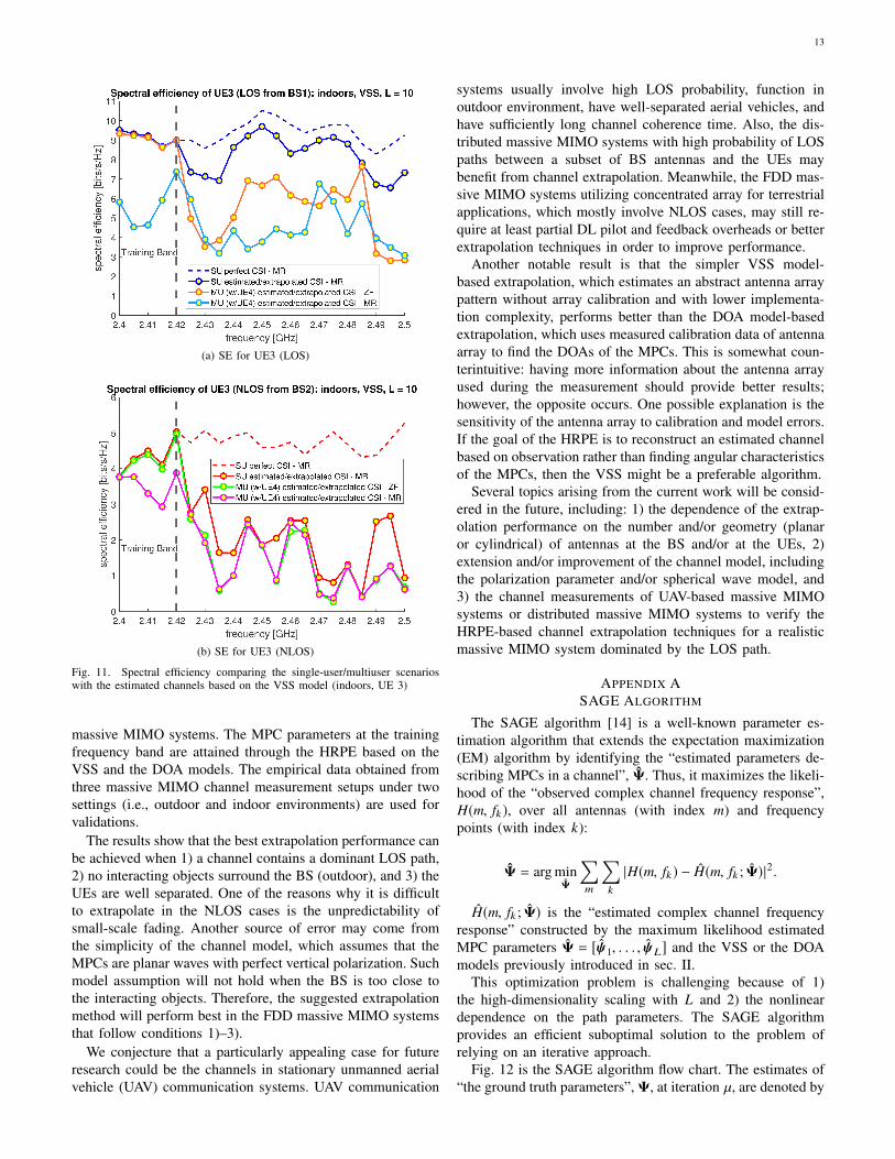
Lastly, Fig. 11 shows the spectral efficiency of UE3 servedby BS1 (LOS) and BS2 (NLOS).6 There are two scenarios:when only the UE3 is served (single-user) and when both UE3and UE4 are served simultaneously (multiuser). Two differentprecodings (i.e., MR and ZF) are used in the multiuser case.

The transmit SNR toward UE n was set toσ

s(n)2

σw(n)

2 = 108 (80dB) assuming 10 dBm transmit power from indoor BS and-70 dBm noise dectected by UE.

6Only the results of the 2.4–2.5 GHz case using the VSS model is plotteddue to space restriction and to their similarity to the DOA results.

The results show that although the single-user performancein the LOS case using the extrapolated channels has smallperformance difference from the perfect CSI (differing byabout 2 bits/s/Hz at maximum), it does not perform as well asin the LOS case under the outdoor environment (as in Fig. 8a).As expected, the extrapolated channel provides large loss inspectral efficiency in the NLOS case. Specifically, the single-user performance and the multiuser performance in the NLOScase are rather similar in the extrapolated bands. Althoughthe ZF provides better than the MR in the LOS case, theyare overlapping in the NLOS case. Overall, extrapolation isdifficult in multiuser scenarios, especially in the NLOS case,whereas it performs relatively better in the single-user LOSscenario.

VI. CONCLUSION

This paper presents the results of our experimental studythat determined the feasibility of channel extrapolation usingthe MPC parameters at a selected training frequency band,with the main goal of eliminating large overheads in FDD

13

(a) SE for UE3 (LOS)

(b) SE for UE3 (NLOS)

Fig. 11. Spectral efficiency comparing the single-user/multiuser scenarioswith the estimated channels based on the VSS model (indoors, UE 3)

massive MIMO systems. The MPC parameters at the trainingfrequency band are attained through the HRPE based on theVSS and the DOA models. The empirical data obtained fromthree massive MIMO channel measurement setups under twosettings (i.e., outdoor and indoor environments) are used forvalidations.

The results show that the best extrapolation performance canbe achieved when 1) a channel contains a dominant LOS path,2) no interacting objects surround the BS (outdoor), and 3) theUEs are well separated. One of the reasons why it is difficultto extrapolate in the NLOS cases is the unpredictability ofsmall-scale fading. Another source of error may come fromthe simplicity of the channel model, which assumes that theMPCs are planar waves with perfect vertical polarization. Suchmodel assumption will not hold when the BS is too close tothe interacting objects. Therefore, the suggested extrapolationmethod will perform best in the FDD massive MIMO systemsthat follow conditions 1)–3).

We conjecture that a particularly appealing case for futureresearch could be the channels in stationary unmanned aerialvehicle (UAV) communication systems. UAV communication

systems usually involve high LOS probability, function inoutdoor environment, have well-separated aerial vehicles, andhave sufficiently long channel coherence time. Also, the dis-tributed massive MIMO systems with high probability of LOSpaths between a subset of BS antennas and the UEs maybenefit from channel extrapolation. Meanwhile, the FDD mas-sive MIMO systems utilizing concentrated array for terrestrialapplications, which mostly involve NLOS cases, may still re-quire at least partial DL pilot and feedback overheads or betterextrapolation techniques in order to improve performance.

Another notable result is that the simpler VSS model-based extrapolation, which estimates an abstract antenna arraypattern without array calibration and with lower implementa-tion complexity, performs better than the DOA model-basedextrapolation, which uses measured calibration data of antennaarray to find the DOAs of the MPCs. This is somewhat coun-terintuitive: having more information about the antenna arrayused during the measurement should provide better results;however, the opposite occurs. One possible explanation is thesensitivity of the antenna array to calibration and model errors.If the goal of the HRPE is to reconstruct an estimated channelbased on observation rather than finding angular characteristicsof the MPCs, then the VSS might be a preferable algorithm.

Several topics arising from the current work will be consid-ered in the future, including: 1) the dependence of the extrap-olation performance on the number and/or geometry (planaror cylindrical) of antennas at the BS and/or at the UEs, 2)extension and/or improvement of the channel model, includingthe polarization parameter and/or spherical wave model, and3) the channel measurements of UAV-based massive MIMOsystems or distributed massive MIMO systems to verify theHRPE-based channel extrapolation techniques for a realisticmassive MIMO system dominated by the LOS path.

APPENDIX ASAGE ALGORITHM

The SAGE algorithm [14] is a well-known parameter es-timation algorithm that extends the expectation maximization(EM) algorithm by identifying the “estimated parameters de-scribing MPCs in a channel”, Ψ. Thus, it maximizes the likeli-hood of the “observed complex channel frequency response”,H(m, fk), over all antennas (with index m) and frequencypoints (with index k):

Ψ = arg minΨ

∑m

∑k

|H(m, fk) − H(m, fk ; Ψ)|2.

H(m, fk ; Ψ) is the “estimated complex channel frequencyresponse” constructed by the maximum likelihood estimatedMPC parameters Ψ = [ψ1, . . . , ψL] and the VSS or the DOAmodels previously introduced in sec. II.

This optimization problem is challenging because of 1)the high-dimensionality scaling with L and 2) the nonlineardependence on the path parameters. The SAGE algorithmprovides an efficient suboptimal solution to the problem ofrelying on an iterative approach.

Fig. 12 is the SAGE algorithm flow chart. The estimates of“the ground truth parameters”, Ψ, at iteration µ, are denoted by

14

Fig. 12. SAGE algorithm flow graph for the VSS model - v can be replaced by d for the DOA model

Fig. 13. Descriptions of the SAGE algorithm steps for the VSS and DOA models

Ψ(µ). The successive ordered cancellation is used to estimatethe initial parameters, Ψ(0), as explained in [14]. At eachiteration, only the parameters corresponding to one path, e.g.,ψv or ψd , are optimized while the parameters for the otherpaths keep their past value (v = µ mod(L)+1). Optimizing theparameters per path reduces the search dimensions by a factorL. A set of L iterations, called an iteration cycle, is requiredto update the parameters for each of the L paths. After aniteration cycle, each path is reestimated based on the updatedvalues of other paths.

Each iteration consists of two steps: 1) the expectationstep and 2) the maximization step. The specific operationsperformed in the two steps in the VSS and DOA algorithmsare shown in Fig. 13. In the expectation step, the interferencedue to the other paths is canceled from the measured channelresponse based on their current estimate. Then, during themaximization step, the parameters ψv or ψd are reestimated.To further reduce the complexity of the problem, the optimiza-tion as a function of the different parameters of each pathis simplified into several 1-D searches over the predefinedparameter grids. This optimizes each parameter at a time,thereby fixing all the other parameters except for the estimatedparameter. The algorithm iterates until convergence or if the

maximum number of iterations is achieved. The implementa-tion is done through MATLAB software.

ACKNOWLEDGMENT

The authors would like to thank A. Adame, A. Alvarado,Z. Cheng, Dr. C. U. Bas, Dr. N. Abbasi, and Dr. D. Burghalfor their assistance in developing the channel sounder, inthe measurement campaigns, and in the productive technicaldiscussions.

REFERENCES

[1] T. Choi et al., “Channel extrapolation for FDD massive MIMO: Proce-dure and experimental results,” in Proc. IEEE 90th Veh. Technol. Conf.(VTC2019-Fall), Sept. 2019, pp. 1–6.

[2] T. L. Marzetta, “Noncooperative cellular wireless with unlimited num-bers of base station antennas,” IEEE Trans. Wireless Commun., vol. 9,no. 11, pp. 3590–3600, Nov. 2010.

[3] T. L. Marzetta, E. G. Larsson, H. Yang, and H. Q. Ngo, Fundamentalsof Massive MIMO. Cambridge University Press, 2016.

[4] E. Björnson, J. Hoydis, and L. Sanguinetti, “Massive MIMO networks:Spectral, energy, and hardware efficiency,” Found. Trends R© SignalProcess., vol. 11, no. 3–4, pp. 154–655, 2017.

[5] E. BjÃurnson, E. G. Larsson, and T. L. Marzetta, “Massive MIMO: Tenmyths and one critical question,” IEEE Commun. Mag., vol. 54, no. 2,pp. 114–123, Feb. 2016.

15

[6] J. Flordelis, F. Rusek, F. Tufvesson, E. G. Larsson, and O. Edfors, “Mas-sive MIMO performanceâATTDD versus FDD: What do measurementssay?” IEEE Trans. Wireless Commun., vol. 17, no. 4, pp. 2247–2261,Apr. 2018.

[7] R. Rogalin et al., “Scalable synchronization and reciprocity calibrationfor distributed multiuser MIMO,” IEEE Trans. Wireless Commun.,vol. 13, no. 4, pp. 1815–1831, Apr. 2014.

[8] J. Vieira, F. Rusek, O. Edfors, S. Malkowsky, L. Liu, and F. Tufvesson,“Reciprocity calibration for massive MIMO: Proposal, modeling, andvalidation,” IEEE Trans. Wireless Commun., vol. 16, no. 5, pp. 3042–3056, May 2017.

[9] X. Jiang, “A framework for over-the-air reciprocity calibration for TDDmassive MIMO systems,” IEEE Trans. Wireless Commun., vol. 17, no. 9,pp. 5975–5990, Sept. 2018.

[10] 3GPP, “Evolved universal terrestrial radio access (E-UTRA); user equip-ment (UE) radio transmission and reception,” 3rd Generation PartnershipProject (3GPP), Technical Specification (TS) 36.101, Oct. 2019, version16.3.0.

[11] F. Rottenberg, R. Wang, J. Zhang, and A. F. Molisch, “Channel ex-trapolation in FDD massive MIMO: Theoretical analysis and numericalvalidation,” in Proc. 2019 IEEE GLOBECOM Conf., Dec. 2019, pp. 1–7.

[12] F. Rottenberg, T. Choi, P. Luo, C. J. Zhang, and A. F. Molisch,“Performance analysis of channel extrapolation in FDD massive MIMOsystems,” IEEE Trans. Wireless Commun., vol. 19, no. 4, pp. 2728–2741,Apr. 2020.

[13] M. D. Larsen, A. L. Swindlehurst, and T. Svantesson, “Performancebounds for MIMO-OFDM channel estimation,” IEEE Trans. SignalProcess., vol. 57, no. 5, pp. 1901–1916, May 2009.

[14] B. H. Fleury, M. Tschudin, R. Heddergott, D. Dahlhaus, and K. IngemanPedersen, “Channel parameter estimation in mobile radio environmentsusing the SAGE algorithm,” IEEE J. Sel. Areas Commun., vol. 17, no. 3,pp. 434–450, March 1999.

[15] X. Rao and V. K. N. Lau, “Distributed compressive CSIT estimationand feedback for FDD multi-user massive MIMO systems,” IEEE Trans.Signal Process., vol. 62, no. 12, pp. 3261–3271, June 2014.

[16] J. Choi, D. J. Love, and P. Bidigare, “Downlink training techniquesfor FDD massive MIMO systems: Open-loop and closed-Loop trainingWith memory,” IEEE J. Sel. Topics Signal Process., vol. 8, no. 5, pp.802–814, Oct. 2014.

[17] Z. Gao, L. Dai, Z. Wang, and S. Chen, “Spatially common sparsity basedadaptive channel estimation and feedback for FDD massive MIMO,”IEEE Trans. Signal Process., vol. 63, no. 23, pp. 6169–6183, Dec. 2015.

[18] A. Adhikary, J. Nam, J. Ahn, and G. Caire, “Joint spatial division andmultiplexingâATthe large-scale array regime,” IEEE Trans. Inf. Theory,vol. 59, no. 10, pp. 6441–6463, Oct. 2013.

[19] Z. Jiang, A. F. Molisch, G. Caire, and Z. Niu, “Achievable rates of FDDmassive MIMO systems with spatial channel correlation,” IEEE Trans.Wireless Commun., vol. 14, no. 5, pp. 2868–2882, May 2015.

[20] B. Lee, J. Choi, J. Seol, D. J. Love, and B. Shim, “Antenna groupingbased feedback compression for FDD-based massive MIMO systems,”IEEE Trans. Commun., vol. 63, no. 9, pp. 3261–3274, Sep. 2015.

[21] B. Lee, H. Ji, D. J. Love, and B. Shim, “Exploiting dominant eigendirec-tions for feedback compression for FDD-based massive MIMO systems,”in Proc. 2016 IEEE Int. Conf. Commun. (ICC), May 2016, pp. 1–6.

[22] Z. Ding and H. V. Poor, “Design of massive-MIMO-NOMA with limitedfeedback,” IEEE Signal Process. Lett., vol. 23, no. 5, pp. 629–633, May2016.

[23] H. Xie, F. Gao, S. Zhang, and S. Jin, “A unified transmission strategy forTDD/FDD massive MIMO systems with spatial basis expansion model,”IEEE Trans. Veh. Technol., vol. 66, no. 4, pp. 3170–3184, Apr. 2017.

[24] H. Liang, W. Chung, and S. Kuo, “FDD-RT: A simple CSI acquisitiontechnique via channel reciprocity for FDD massive MIMO downlink,”IEEE Syst. J., vol. 12, no. 1, pp. 714–724, Mar. 2018.

[25] W. Shen, L. Dai, B. Shim, Z. Wang, and R. W. Heath, “Channel feedbackbased on AoD-adaptive subspace codebook in FDD massive MIMOsystems,” IEEE Trans. Commun., vol. 66, no. 11, pp. 5235–5248, Nov.2018.

[26] M. Alrabeiah and A. Alkhateeb, “Deep learning for TDD and FDDmassive MIMO: Mapping channels in space and frequency,” arXiv e-prints, p. arXiv:1905.03761, May 2019.

[27] Y. Liao, H. Yao, Y. Hua, and C. Li, “CSI feedback based on deeplearning for massive MIMO systems,” IEEE Access, vol. 7, pp. 86 810–86 820, June 2019.

[28] Y. Yang, F. Gao, G. Y. Li, and M. Jian, “Deep learning-based downlinkchannel prediction for FDD massive MIMO system,” IEEE Commun.Lett., vol. 23, no. 11, pp. 1994–1998, Nov. 2019.

[29] M. Pun, A. F. Molisch, P. Orlik, and A. Okazaki, “Super-resolution blindchannel modeling,” in Proc. 2011 IEEE ICC, June 2011, pp. 1–5.

[30] W. Yang, L. Chen, and Y. E. Liu, “Super-resolution for achievingfrequency division duplex (FDD) channel reciprocity,” in Proc. 2018IEEE 19th Int. Wksh SPAWC, June 2018, pp. 1–5.

[31] U. Ugurlu, R. Wichman, C. B. Ribeiro, and C. Wijting, “A multipathextraction-based CSI acquisition method for FDD cellular networks Withmassive antenna arrays,” IEEE Trans. Wireless Commun., vol. 15, no. 4,pp. 2940–2953, Apr. 2016.

[32] X. Zhang, L. Zhong, and A. Sabharwal, “Directional training for FDDmassive MIMO,” IEEE Trans. Wireless Commun., vol. 17, no. 8, pp.5183–5197, Aug. 2018.

[33] N. Jalden, H. Asplund, and J. Medbo, “Channel extrapolation based onwideband MIMO measurements,” in Proc. 2012 6th EUCAP, Mar. 2012,pp. 442–446.

[34] D. Vasisht, S. Kumar, H. Rahul, and D. Katabi, “Eliminating channelfeedback in Next-Generation cellular networks,” in Proc. 2016 ACMSIGCOMM Conf., Aug. 2016, pp. 398–411.

[35] M. Arnold, S. DÃurner, S. Cammerer, S. Yan, J. Hoydis, and S. Brink,“Enabling FDD massive MIMO through deep learning-based channelprediction,” arXiv e-prints, p. arXiv:1901.03664, Jan. 2019.

[36] J. Hong, J. Rodrà guez-PiÃseiro, and X. Yin, “FDD Channel infer-ence methods with experimental performance evaluation,” IEEE Access,vol. 8, pp. 10 491–10 502, Jan. 2020.

[37] H. Krim and M. Viberg, “Two decades of array signal processingresearch: The parametric approach,” IEEE Signal Process. Mag., vol. 13,no. 4, pp. 67–94, July 1996.

[38] J. Medbo and F. Harrysson, “Efficiency and accuracy enhanced superresolved channel estimation,” in Proc. 2012 6th EUCAP, Mar. 2012, pp.16–20.

[39] R. Schmidt, “Multiple emitter location and signal parameter estimation,”IEEE Trans. Antennas Propag., vol. 34, no. 3, pp. 276–280, Mar. 1986.

[40] R. Roy and T. Kailath, “ESPRIT-estimation of signal parameters viarotational invariance techniques,” IEEE Trans. Acoustics, Speech, SignalProcess., vol. 37, no. 7, pp. 984–995, July 1989.

[41] J. A. Hogbom, “Aperture synthesis with a non-regular fistribution ofinterferometer baselines,” Astron. Astrophys. Suppl. Ser., vol. 15, pp.417–426, June 1974.

[42] A. Richter, Estimation of Radio Channel Parameters: Models andAlgorithms. ISLE, 2005.

[43] M. Friese, “Multitone signals with low crest factor,” IEEE Trans.Commun., vol. 45, no. 10, pp. 1338–1344, Oct. 1997.