Phys 275 - June 2021 119

Experiment XI Standing Waves

I. Purpose The purpose of this lab is to investigate the behavior of waves in a simple system, a wire with fixed points at both ends. If you drive the wire at certain specific frequencies, a standing wave with relatively large amplitude will be produced. These frequencies are resonances of the system and have many similarities to the resonance you observed in the forced harmonic motion apparatus. You will find the resonant frequencies, determine how they depend on the parameters of the system, see how to find the weighted average of several measurements, and compare your results to a simple theory.

II. Preparing for the Lab This is not a simple experiment and you will need to prepare before attempting this lab. Although you may think wave phenomena are simple, the experimental set-up is not. Also non-linear effects are readily observable in this set-up, which are beyond the scope of your introductory physics courses. The Introduction below provides a brief review of a few basic results on waves that you will need. This is a complex lab and you need to read the entire write-up before you get to the lab so that you understand what needs to be done. For example, in Part C you will find the weighted average, which is not an easy concept. Before you go to the lab, read the references on the weighted average and make sure you understand how to compute the “weight” of a data point. Finally, don’t forget to complete the Pre-Lab questions on Expert TA before your lab starts.

III. References For more on the physics of waves see Appendix E, your Physics 273 textbook, or “Waves - Berkeley Physics Course Volume 3” by Frank Crawford. For how to find the weighted average, see Appendix A of this lab manual, or page 31 from Lyon, or Chapter 7 from Taylor. For more on using the oscilloscope, see Appendix G.

IV. Prelab Questions #1. A wire is fixed at both ends, with 1.500 m between the fixed points. Assume there is a total

mass of 0.200 kg hanging on the end of the wire, the mass per unit length of the wire is 0.00080 kg/m, and the acceleration due to gravity is g=9.80102 m/s2.

(a) What is the speed of waves propagating on the wire? (b) What is the wavelength of the lowest frequency mode? (c) What is the frequency of the lowest frequency mode, i.e. the n=1 mode? #2. If the fundamental mode of a wire is at 28 Hz, what is the frequency of the next (n=2) mode? #3. If you increase the tension in the wire by a factor of 2, will the frequency of the lowest

frequency mode (a) decrease by a factor of 2, (b) decrease by a factor of 2 , (c) not change, (d) increase by a factor of 2 , (e) increase by a factor of 2, (f) increase by a factor of 4.

#4. In Figure 2, the magnetic field goes from the North pole (red) to the South (blue) pole of the magnet. When the supply voltage Vs > 0, current I > 0 will flow down the wire from left to right. What is the direction of the force the magnet exerts on the wire?

#5. Suppose you measure frequencies 23 ± 1Hz, 24 ± 0.5 Hz, 24.5 ± 0.3 Hz, and 25 ± 0.25 Hz. (a) What is the weighted average of these frequencies (see Appendix A)? (b) What is the uncertainty in the weighted average of these frequencies?

Phys 275 - June 2021 120

V. Introduction This experiment involves the driven motion of a wire with two fixed ends. The wire is driven by an oscillating force that you will be able to adjust in amplitude and frequency. At certain well-defined drive frequencies, you will find that standing waves are formed with relatively large amplitude. You will test a simple theory that predicts that these natural oscillation frequencies form a regularly spaced sequence with the frequency interval determined by the length L of the wire, the tension T in the wire and the wire's mass per unit length µ. The simple theory of mechanical waves on a wire or string is covered in Appendix E of this manual. This theory gives two different equations for the phase velocity vs of waves on a wire:

vs =Tµ

and vs = λ f (1)

The second equation can be substituted into the first, eliminating the velocity, to get:

λ f =Tµ

(2)

If both ends of the wire are kept fixed, resonant standing waves will occur when the wavelengths satisfy: λ =

2 Ln

(3)

where n = 1, 2, 3, 4… is an integer. Substituting this into Equation [2] and rearranging gives:

1/212

nf Tn L µ

=

or 1/2

2nnf T

L µ

=

(4)

Where fn is the frequency of the nth harmonic. Equation (4) can also be written as:

nTL

fn

=

µ21 , (5)

which shows that the frequency fn of the n-th harmonic is linearly proportional to n. The different standing waves not only occur at different frequencies, but the wavelength decreases with mode number n (see Eq. (3)). Figure 1 shows snapshots of the displacement y versus position x along the wire produced by the n=1, 2 and 3 modes. The apparatus you will be using consists of a wire that is fixed at one end, while the other end passes over another fixed point to a pulley and then to a hanger that holds a mass M. The hanger applies tension T= Mg. The mass M can be varied, allowing the tension T to be varied. The wire is driven by the Lorentz force F I B= × that results from the interaction of an oscillating

Figure 1. Snapshots at fixed time showing three lowest frequency standing waves on a string held fixed x = 0 and 1.0 m. The fundamental mode n=1 (blue) has one anti-node (place of maximum displacement). The n=2 mode (red) has 2 anti-nodes and mode n=3 (green) has 3 anti-nodes.

Phys 275 - June 2021 121

current I flowing in the wire and the magnetic field B in the wire section of length between the North and South poles of a permanent magnet (see Figure 2). The function generator supplying the ac current has a frequency and amplitude output that you can tune manually and monitor with an oscilloscope. The scope also monitors the output from a photogate sensor that can measure very small displacements of the wire. VI. Equipment standing wave apparatus with function generator photogate sensor and power supply 2-channel oscilloscope meter stick LabPro LinFit and LnLnfit Excel spreadsheets Waves LoggerPro Template.cmbl Waves-Excel Template-Exp 11 VII. Experimental Procedure and Analysis Part A: Setting up the Apparatus

1. Go to the Excel Templates folder on the Desktop and open Waves-Excel Template-Exp 11.

Save a copy in the Documents folder with your name in the title. 2. Measure the mass mo of the wire sample that is kept at the front of the lab, which has a length

of Lo=2.000 m ± 2 mm, and record in the first worksheet. Also estimate the uncertainty σmo in the wire mass m.

QUESTION A2: Compute the mass density µ and the uncertainty σµ in the mass density µ. Make sure you use SI units in this lab - meters, kilograms and seconds!

3. Add weight to the hanger (see Figure 2) so that the wire is supporting a total mass of M = 0.200

kg. Note: since the holder has a 0.050 kg mass, this means you need to add 0.150 kg - double check that you actually have a total mass of 0.200 kg. Record the tension T = Mg in your spreadsheet.

4. For best results, the wire should be a bit shorter than 1 m long between the two fixed points.

That way you can use a 1 meter ruler to measure the length. Make sure the fixed points are pushed up against the clamps so they won’t move. Measure the Length L of the wire between the fixed points and record L and its uncertainty in your spreadsheet.

QUESTION A1: A wire of length Lo has mass mo and linear mass density µ = mo/Lo. Assume that σmo is the uncertainty in mo and σLo is the uncertainty in Lo. In the space below or on a separate piece of paper, use propagation of errors and simplify to find an equation for the uncertainty σµ in µ.

Phys 275 - June 2021 122

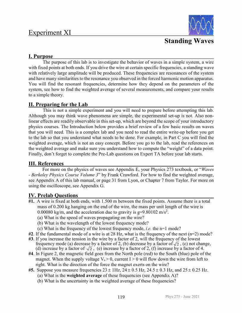
(a) (b) Figure 2. (a) Photo of wave apparatus showing wire going between N (red) and S (blue) poles of magnet. (b) Circuit schematic shows moving wire connected in series with function generator voltage supply Vs and 10 Ω resistor. Wire is driven by Lorentz force from current in wire as it goes through magnet. Position of the wire is measured using an LED and optical sensor. Channel 1 of the scope measures ac drive voltage Vs while Channel 2 measures voltage output Vyopt from optical sensor, which is proportional to the wire’s displacement y at the location of the sensor. Output voltage Vs from function generator and output voltage Vyopt from optical sensor are monitored by the Vernier LabPro box, which digitizes and transfers signals to the computer using Logger Pro.

Phys 275 - June 2021 123

(a) (b)

Figure 3. (a) Channel 1 and Channel 2 inputs and control panel on right side of oscilloscope. (b) Display panel on the left side of the scope after the Measure button was pushed.

5. The magnet should have the North pole (red) closest to you when you face the apparatus (see

Fig. 2) and be placed near one end of the wire. Also check that the wire centered in the gap between the two pole faces.

6. Turn on the photogate power supply. Examine the circuit and setup diagram shown in Figure 2.

Verify that your apparatus is set up as in Figure 2 and check in particular that the wire, 10 Ω resistor, and function generator are connected to form a closed circuit.

7. Turn on the oscilloscope (on-button is on top of scope) and let it go through automated set-up. 8. Turn on the function generator, set the frequency range switch to the 1-100 Hz range and the

waveform to Sine wave. Adjust the amplitude knob to about the 9 or 10 o’clock position which will generate between 0.5 V and 1 V.

Phys 275 - June 2021 124

Safety Note: Do not set the function generator amplitude beyond the 12 o’clock setting or the 10 Ω resistor can get hot enough to burn you.

9. Push the Ch 1 Menu button (see Fig. 3(a)) and use the soft-keys to set scope channel 1 AC

coupled and BW limit: On. Do the same for Ch 2. Next push the Trigger Menu button (see Fig. 3(a)) and verify that the trigger is set to:

Trigger Source: Ch 1 Slope: Rising Coupling: HF Reject Mode: Normal Verify that Ch 1 shows the sine wave drive from the oscillator and that a trace is visible for Ch

2 (just a flat line might be visible at this point). Adjust the Vertical knobs for both channels and the Horizontal knob and to get a nice looking display.

10. Push the Measure button on the scope and use the soft-keys to set the scope so it is displaying

the peak-to-peak voltages of Ch 1 and Ch 2 and the frequency of channel 1 (see Fig. 3(b)). 11. Carefully examine the apparatus and then take a picture using the web camera. Paste the

picture into your spreadsheet. Part B: Collect Some Data of fn versus n 1. With a total mass of M = 0.200 kg on the end of the wire, adjust the frequency of the function

generator supply until you see a resonance response at the fundamental frequency. This is typically in the 20 Hz to 30 Hz range. The wire tends to oscillate in either a "vertical mode" or a "circular mode". For most set-ups, only circular modes are visible for higher harmonics. When you have found the frequency at which the response is largest, read the frequency from the scope (use the measure button) and record in the designated area in the first worksheet in your spreadsheet template. Then find and record the resonant frequency fn for the next four harmonics so that in the end you have fn for n=1, 2, 3, 4, 5. Include proper units (Hz).

2. Estimate the uncertainty in each of your measurements of fn. To do this, note that two things

can cause uncertainty in your fn values. First, you should see that the frequencies reported by the scope are fluctuating. To find this part of the uncertainty, record a few values reported by the scope and take the standard deviation. Second, if you try to tune to the same resonance a second time, you may arrive at a different frequency. To quantify this part of the uncertainty, retune and measure fn two or three times (just pick one scope reading at each attempt, don’t average multiple scope readings together). It is unlikely that you will find an identical frequency each time you retune and you can just take the standard deviation of a few measurements to find the uncertainty. Since this last standard deviation will have uncertainty from the fluctuating scope readings and from the difficulty in locating the resonance and any drift in the resonance, it is a good estimate of the actual overall uncertainty in fn.

3. Make a plot of the frequency fn versus the mode number n and show your instructor. Be sure to

label your plot axes, don’t forget to add units, and add a title - Plot B: Frequency vs Mode #.

Phys 275 - June 2021 125

Part C: Linear Analysis and Weighted Mean 1. To see if your fn data scales linearly with n, as predicted by Equation (5), go to the Excel

Templates folder and LinFit 3 (do not confuse it with LnLnFit 3). LinFit 3 contains a Macro for automatically fitting data to a straight line xaay 10 += . It gives you the best fit slope a1 and best fit intercept ao and also finds the uncertainty in the slope and intercept. Put the fn values into the column labelled “y” and the n values into the column labelled “x”. You also need to put the uncertainties in frequency σfn in the column labelled σy. The n values have no uncertainty so you should leave the column for σx empty.

2. After you have entered all the data into LinFit 3, click on the gray Macro button. It will ask if

you want to force the intercept ao to zero, click Yes, which is what Equation (5) implies. 3. After you run LinFit 3, copy everything in it (title cell, data, errors, and fitting results) except

for the macro button and paste a copy into the first worksheet in your spreadsheet. QUESTION C1: Is the resonant frequency fn consistent with being linearly proportional to the harmonic number n? QUESTION C2: How did you determine you answer to Question C1? 4. For each of your measured values fn calculate fn /n and the uncertainty in fn /n.

5. Now fill in the rest of the template for Part C and calculate the weighted mean <fn /n> and the

uncertainty in the weighted mean (see Equations A.14 and A.15 in Appendix A). QUESTION C3: Compare the value you found for the weighted mean <fn /n> to the value LinFit 3 found for a1. Also compare your value for the uncertainty in the weighted mean to the value LinFit 3 obtained for σa1. Use complete sentences and clearly state each value obtained.

Part D: Resonant Response of the wire 1. Turn on the power to the optical gate. The optical gate should already have been set up properly,

so that motion of the wire up or down causes the output voltage Vyopt to change. Sometimes things get moved around though, so check that the optical gate is on the opposite end of the wire from the magnet (see Figure 2(a)) and no more than 3” away from the fixed point.

2. Adjust the scope’s CH 1 and CH 2 vertical scales and offsets so that both traces are centered in

the display. 3. Place a total mass of 0.200 kg on the wire. Turn the amplitude knob on the function generator

drive until CH 1 shows it is supplying a sine wave with a peak-to-peak voltage of 200 mV to 400 mV. Note: At the higher end of this range, non-linear effects will be more obvious.

4. Adjust the function generator frequency to drive the fundamental mode at its resonance.

Phys 275 - June 2021 126

Figure 4. (a) Photograph of wire going through optical gate. Turning y-knob clockwise one full rotation moves gate upward by 0.5 mm with respect to the wire. (b) For proper operation the wire should be midway between the optical sensor and LED (infrared light source) and about 0.8 mm higher than the center of the sensor. If the wire then moves higher, it blocks less light and the sensor outputs more voltage, while if the wire moves lower, it blocks more light and the sensor outputs less voltage. The motion can only be faithfully measured if the wire moves less than about 0.8 mm up or down. The sensitivity of the sensors varies considerably, but typically if the wire moves by 0.4 mm, the optical output voltage should change by roughly 0.1 V. 5. The scope should now be showing two sinusoidal curves with the same frequency; Ch 1 is the

drive voltage and Ch 2 is the output voltage Vyopt from the optical sensor, which gives an output that is directly related to the wire’s y-position at the gate. If you see two sine waves, adjust the horizontal and vertical scales on the scope to get a nice display. If you do not see a sine wave on CH 2, make sure the function generator is set to the first resonance frequency and the output is in the 200-400 mV range. If you see a distorted sine wave on CH 2, check that the function generator is not applying more than 400 mV peak-to-peak and the gate is no more than 3” from the fixed point. Then try turning the drive voltage down to 200 mV peak-to-peak. If the distortion is small, you can try turning the y-knob (see Figure 4 (a)) by a little bit (less than a full rotation) and see if the CH 2 output becomes a nice sine wave. If you still don’t see a good output, the gate height may need to be adjusted and you will need to get your instructor.

6. Adjust the scope so that you can clearly see the signal from both channels. 7. Have your instructor verify that you have set everything up correctly - especially the optical

gate. Do not go past this point unless your instructor has checked that everything is OK. 8. Go to the LoggerPro folder and open “Waves LoggerPro Template.cmbl”. Figure 5 shows the

layout for this panel, which is similar to the one you used for the forced harmonic motion experiment. Click Collect to acquire 0.2 s of Ch 1 and Ch 2 data at 1000 samples/s.

9. Note how this LoggerPro template automatically fits the data in each channel to a sine wave and

displays the fit parameters including the amplitude (which it calls A), the frequency (B) and the phase (D). Verify that the fit curves (thin black curves) in the top two panels look like they are close fits to the data. If they are not close fits to the data, try clicking on and moving the [ or ] symbols on the plot which define the region being fitted.

Phys 275 - June 2021 127

Figure 5. Display panel for LoggerPro Waves Template. 10. Looking at the scope Ch 2, tune the function generator to the fundamental frequency. Then

have LoggerPro collect the drive voltage (Ch 1) and voltage output Vyopt from the optical gate (Ch 2) versus time. Click on the box with the fit parameters for the source voltage Vdrive and copy (Ctlr C). Then go to Part D in you spreadsheet and paste (Ctrl V) into the location that is highlighted in yellow and says ”click here and paste Auto Fit Vdrive table”. Do the same for the fit parameters for Vyopt. This gets the fit parameters A, B, C, D into your spreadsheet template. Also select all of the t, Vs and Vyopt data in LoggerPro and paste into the designated spot in your spreadsheet template. The template will automatically plot the data and fit for Vs(t) and Vyopt(t).

11. Once you have pasted in your data for the resonance, the template will generate a list of target

frequencies, which are in a tight range near the resonance. Repeat the previous step for the 7 additional target frequencies listed in the template.

12. Once you have filled in all the measurements, your spreadsheet will finish making plots of the

amplitude versus frequency and phase versus frequency. Examine these plots to answer the following questions.

Question D1 - Using the result Q = f1/∆f from Experiment 10-Forced Harmonic Motion, where ∆f

is the full width of the peak at 1/ 2 0.707= of the maximum, what is the approximate Q of the wire’s fundamental resonance?

Question D2 - By how much does the phase change when you sweep through the resonance? Question D3 - How does your answer to Question D2 compare to the total phase change when

you sweep through the resonance in a simple harmonic oscillator (as in Experiment 10).

Phys 275 - June 2021 128

Part E: Frequency versus Tension 1. In this part you will be measuring the frequency versus tension in the wire to see if it obeys

Equation [5]. To get good data for this part, you need to: (a) use a very low amplitude driving voltage, (b) use the optical gate to observe the wire’s resonant response, and (c) make sure that static friction is not present between the wire and its fixed point.

2. Set the drive voltage to 75-100 mV peak-to-peak. Now measure the second harmonic frequency

f2 for 8 different tensions T= Mg using total masses of 0.050, 0.100, 0.150, 0.200, 0.250, 0.300, 0.350 and 0.400 kg. Note: after you place a mass on the hanger, you need to remove static friction between the wire and the fixed point closest to the weight, do this by lifting the wire off the fixed point near the optical gate and gently placing it back down on the fixed point. Record your data in the third worksheet in the Excel Template.

3. Make a plot showing f2 versus the tension T for your 8 measurements. 4. Next check if your data follows Equation [5] for n=2,

12

21f T

L µ

=

, [6]

To do this, go to the Excel Templates folder and find LnLnFit 3 which fits data to the function y = a0 xa1 . So if you let y = f2, σy = σf2 and x=T=Mg you can do the fit and find a0 and a1. For this part you can neglect the uncertainties in the tension T.

QUESTION E1: Is the value you got for a1 consistent with the expected value of a1=1/2 from the theory? Explain how you got the answer.

5. Comparing the fitting function y = a0 xa1 to Equation [4] with n=2, you can show that

01a

L µ= . [7]

Solving this equation for µ gives 2 2 2 21/ o oL a L aµ − −= = [8]

Use Equation [8] to determine µ from ao. 6. Use propagation of errors on Equation [8] to find the uncertainty σµ in µ.

QUESTION E2: Is the value for µ that you obtained in Step 5 consistent with the value you reported in Question A2? Explain how you determined the answer to this question.

Phys 275 - June 2021 129

VIII. Finishing Up

Save your spreadsheet and submit it to ELMS before you leave the Lab. Turn in your checksheet to your instructor before you leave. If you did not complete the entire lab in class, finish everything at home and submit a revised spreadsheet to ELMS before the due date, which is typically by the start of your next lab. If you finished early, use the remaining class time to work on the Homework or look over the next lab and work on the Pre-lab Questions.

IX. Homework (Submit your answers to the homework to Expert TA before the deadline) Questions and multiple choice answers on Expert TA may vary from those given below. Be sure

to read questions and choices carefully before submitting your answers on Expert TA.

#1. Suppose that you measured harmonic frequencies fn of 23 Hz, 48 Hz, 73 Hz, and 101 Hz for n = 1, 2, 3, 4 with an uncertainty of 1 Hz in each frequency measurement.

(a) Find the weighted average of fn/n. (b) What is the uncertainty in the weighted average of these frequencies? #2. (a) What was the mass per unit length of the wire used in this experiment? (b) How much tension would you need to apply to the wire in this experiment in order for the

wave speed to equal the speed of sound in air (assume 340 m/s)? (c) What is the total mass you would need to hang on the end of the wire to get the tension

found in part (b) of this problem? #3. In Appendix E, it is stated that y=f(x±vst) is the general solution to the wave equation E.1

when f is ANY well-behaved function of x±vst. Show that this is true by substituting into Equation E.1 and working out the derivatives.

#4. Did you find that the mass density you predict from fitting the frequencies differed

significantly from the measured mass density? In complete sentences, consider what might be causing this discrepancy and suggest an experiment you could do to test your ideas.

#5H. [This Question is for Hotshots Only] Suppose the optical gate in this setup gives a

sensitivity to motion of the wire of about 0.25 V/mm (see Figure 4). With some averaging on the scope (an advanced scope function that we don’t use in class), the electrical noise level can be reduced to about 0.25 mV. What is the smallest motion of the wire that can be detected?