Data Min Knowl Disc (2007) 15:107–144DOI 10.1007/s10618-007-0064-z

Experiencing SAX: a novel symbolic representationof time series

Jessica Lin · Eamonn Keogh · Li Wei ·Stefano Lonardi

Received: 15 June 2006 / Accepted: 10 January 2007 / Published online: 3 April 2007Springer Science+Business Media, LLC 2007

Abstract Many high level representations of time series have been proposedfor data mining, including Fourier transforms, wavelets, eigenwaves, piecewisepolynomial models, etc. Many researchers have also considered symbolic rep-resentations of time series, noting that such representations would potentialityallow researchers to avail of the wealth of data structures and algorithms fromthe text processing and bioinformatics communities. While many symbolic rep-resentations of time series have been introduced over the past decades, they allsuffer from two fatal flaws. First, the dimensionality of the symbolic represen-tation is the same as the original data, and virtually all data mining algorithmsscale poorly with dimensionality. Second, although distance measures can bedefined on the symbolic approaches, these distance measures have little corre-lation with distance measures defined on the original time series.

In this work we formulate a new symbolic representation of time series. Ourrepresentation is unique in that it allows dimensionality/numerosity reduction,

Responsible editor: Johannes Gehrke.

J. Lin (B)Information and Software Engineering Department, George Mason University, Fairfax,VA 22030, USAe-mail: jessica@ise.gmu.edu

E. Keogh · L. Wei · S. LonardiComputer Science & Engineering Department, University of California-Riverside, Riverside,CA 92521, USAe-mail: eamonn@cs.ucr.edu

L. Weie-mail: wli@cs.ucr.edu

S. Lonardie-mail: stelo@cs.ucr.edu

108 J. Lin et al.

and it also allows distance measures to be defined on the symbolic approach thatlower bound corresponding distance measures defined on the original series.As we shall demonstrate, this latter feature is particularly exciting because itallows one to run certain data mining algorithms on the efficiently manipulatedsymbolic representation, while producing identical results to the algorithmsthat operate on the original data. In particular, we will demonstrate the utilityof our representation on various data mining tasks of clustering, classification,query by content, anomaly detection, motif discovery, and visualization.

Keywords Time series · Data mining · Symbolic representation · Discretize

1 Introduction

Many high level representations of time series have been proposed for data min-ing. Figure 1 illustrates a hierarchy of all the various time series representationsin the literature (Andre-Jonsson and Badal 1997; Chan and Fu 1999; Faloutsoset al. 1994; Geurts 2001; Huang and Yu 1999; Keogh et al. 2001a; Keogh andPazzani 1998; Roddick et al. 2001; Shahabi et al. 2000; Yi and Faloutsos 2000).One representation that the data mining community has not considered in detailis the discretization of the original data into symbolic strings. At first glance thisseems a surprising oversight. There is an enormous wealth of existing algorithmsand data structures that allow the efficient manipulations of strings. Such algo-rithms have received decades of attention in the text retrieval community, andmore recent attention from the bioinformatics community (Apostolico et al.2002; Durbin et al. 1998; Gionis and Mannila 2003; Reinert et al. 2000; Stadenet al. 1989; Tompa and Buhler 2001). Some simple examples of “tools” that arenot defined for real-valued sequences but are defined for symbolic approachesinclude hashing, Markov models, suffix trees, decision trees, etc.

There is, however, a simple explanation for the data mining community’slack of interest in string manipulation as a supporting technique for miningtime series. If the data are transformed into virtually any of the other repre-sentations depicted in Fig. 1, then it is possible to measure the similarity of twotime series in that representation space, such that the distance is guaranteed tolower bound the true distance between the time series in the original space.1

This simple fact is at the core of almost all algorithms in time series data miningand indexing (Faloutsos et al. 1994). However, in spite of the fact that there aredozens of techniques for producing different variants of the symbolic represen-tation (Andre-Jonsson and Badal 1997; Daw et al. 2001; Huang and Yu 1999),there is no known method for calculating the distance in the symbolic space,while providing the lower bounding guarantee.

In addition to allowing the creation of lower bounding distance measures,there is one other highly desirable property of any time series representation,

1 The exceptions are random mappings, which are only guaranteed to be within an epsilon of thetrue distance with a certain probability, trees, interpolation and natural language.

Experiencing SAX: a novel symbolic representationof time series 109

Time Series RepresentationsData Adaptive Non Data Adaptive

SpectralWavelets PiecewiseAggregate

Approxima tion

PiecewisePolynomial

SymbolicSingularValue

Decompos ition

RandomMappings

Piecewise LinearApproximation

Adaptive PiecewiseConstant

Approximation

DiscreteFourier

Transform

DiscreteCosine

TransformHaar Daubechies

dbn n > 1Coiflets Symlets

Sorted Coe fficients

Orthonormal Bi-Orthonormal

Interpolatio n Regression

Trees

NaturalLanguage

Strings

LowerBounding

Non- LowerBounding

Fig. 1 A hierarchy of all the various time series representations in the literature. The leaf nodesrefer to the actual representation, and the internal nodes refer to the classification of the approach.The contribution of this paper is to introduce a new representation, the lower bounding symbolicapproach

including a symbolic one. Almost all time series datasets are very high dimen-sional. This is a challenging fact because all non-trivial data mining and indexingalgorithms degrade exponentially with dimensionality. For example, above 16–20 dimensions, index structures degrade to sequential scanning (Hellersteinet al. 1997). None of the symbolic representations that we are aware of allowdimensionality reduction (Andre-Jonsson and Badal 1997; Daw et al. 2001;Huang and Yu 1999). There is some reduction in the storage space required,since fewer bits are required for each value; however, the intrinsic dimension-ality of the symbolic representation is the same as the original data.

There is no doubt that a new symbolic representation that remedies allthe problems mentioned above would be highly desirable. More specifically,the symbolic representation should meet the following criteria: space effi-ciency, time efficiency (fast indexing), and correctness of answer sets (no falsedismissals).

In this work we formally formulate a novel symbolic representation andshow its utility on other time series tasks.2 Our representation is unique inthat it allows dimensionality/numerosity reduction, and it also allows distancemeasures to be defined on the symbolic representation that lower bound corre-sponding popular distance measures defined on the original data. As we shalldemonstrate, the latter feature is particularly exciting because it allows oneto run certain data mining algorithms on the efficiently manipulated symbolicrepresentation, while producing identical results to the algorithms that operateon the original data. In particular, we will demonstrate the utility of our repre-sentation on the classic data mining tasks of clustering (Kalpakis et al. 2001),classification (Geurts 2001), indexing (Agrawal et al. 1995; Faloutsos et al. 1994;Keogh et al. 2001a; Yi and Faloutsos 2000), and anomaly detection (Dasguptaand Forrest 1999; Keogh et al. 2002; Shahabi et al. 2000).

The rest of this paper is organized as follows. Section 2 briefly discussesbackground material on time series data mining and related work. Section 3introduces our novel symbolic approach, and discusses its dimensionality reduc-tion, numerosity reduction and lower bounding abilities. Section 4 contains anexperimental evaluation of the symbolic approach on a variety of data mining

2 A preliminary version of this paper appears in Lin et al. (2003).

110 J. Lin et al.

tasks. Impact of the symbolic approach is also discussed. Finally, Section 5 offerssome conclusions and suggestions for future work.

2 Background and Related Work

Time series data mining has attracted enormous attention in the last decade.The review below is necessarily brief; we refer interested readers to (Keoghand Kasetty 2002; Roddick et al. 2001) for a more in depth review.

2.1 Time series data mining tasks

While making no pretence to be exhaustive, the following list summarizes theareas that have seen the majority of research interest in time series data mining.

• Indexing: Given a query time series Q, and some similarity/dissimilarity mea-sure D(Q,C), find the most similar time series in database DB (Agrawalet al. 1995; Chan and Fu 1999; Faloutsos et al. 1994; Keogh et al. 2001a; Yiand Faloutsos 2000).

• Clustering: Find natural groupings of the time series in database DB undersome similarity/dissimilarity measure D(Q,C) (Kalpakis et al. 2001; Keoghand Pazzani 1998).

• Classification: Given an unlabeled time series Q, assign it to one of two ormore predefined classes (Geurts 2001).

• Summarization: Given a time series Q containing n datapoints where n isan extremely large number, create a (possibly graphic) approximation of Qwhich retains its essential features but fits on a single page, computer screen,executive summary etc (Lin et al. 2002).

• Anomaly detection: Given a time series Q, and some model of “normal”behavior, find all sections of Q which contain anomalies or“surprising/interesting/unexpected/novel” behavior (Dasgupta and Forrest1999; Keogh et al. 2002; Shahabi et al. 2000).

Since the datasets encountered by data miners typically don’t fit in main mem-ory, and disk I/O tends to be the bottleneck for any data mining task, a simplegeneric framework for time series data mining has emerged (Faloutsos et al.1994). The basic approach is outlined in Table 1.

It should be clear that the utility of this framework depends heavily on thequality of the approximation created in Step 1. If the approximation is veryfaithful to the original data, then the solution obtained in main memory is likelyto be the same as, or very close to, the solution we would have obtained on theoriginal data. The handful of disk accesses made in Step 3 to confirm or slightlymodify the solution will be inconsequential compared to the number of diskaccesses required had we worked on the original data. With this in mind, therehas been great interest in approximate representations of time series, which weconsider below.

Experiencing SAX: a novel symbolic representationof time series 111

Table 1 A generic time seriesdata mining approach

1. Create an approximation of the data, whichwill fit in main memory, yet retains the essen-tial features of interest.

2. Approximately solve the task at hand inmain memory.

3. Make (hopefully very few) accesses to theoriginal data on disk to confirm the solutionobtained in Step 2, or to modify the solutionso it agrees with the solution we would haveobtained on the original data.

0 50 100 0 50 1000 50 1000 50 100

Discrete Fourier Transform

Piecewise Linear Approximation

Haar Wavelet Adaptive PiecewiseConstant Approximation

Fig. 2 The most common representations for time series data mining. Each can be visualized as anattempt to approximate the signal with a linear combination of basis functions

2.2 Time series representations

As with most problems in computer science, the suitable choice of representa-tion greatly affects the ease and efficiency of time series data mining. With thisin mind, a great number of time series representations have been introduced,including the Discrete Fourier Transform (DFT) (Faloutsos et al. 1994), theDiscrete Wavelet Transform (DWT) (Chan and Fu 1999), Piecewise Linear,and Piecewise Constant models (PAA) (Keogh et al. 2001a), (APCA) (Geurts2001; Keogh et al. 2001a), and Singular Value Decomposition (SVD) (Keoghet al. 2001a). Figure 2 illustrates the most commonly used representations.

Recent work suggests that there is little to choose between the above interms of indexing power (Keogh and Kasetty 2002); however, the representa-tions have other features that may act as strengths or weaknesses. As a simpleexample, wavelets have the useful multiresolution property, but are only definedfor time series that are an integer power of two in length (Chan and Fu 1999).

One important feature of all the above representations is that they are realvalued. This limits the algorithms, data structures and definitions available forthem. For example, in anomaly detection we cannot meaningfully define theprobability of observing any particular set of wavelet coefficients, since theprobability of observing any real number is zero (Larsen and Marx 1986). Suchlimitations have lead researchers to consider using a symbolic representationof time series.

112 J. Lin et al.

While there are literally hundreds of papers on discretizing (symbolizing,tokenizing, quantizing) time series (Andre-Jonsson and Badal 1997; Huang andYu 1999) (see (Daw et al. 2001) for an extensive survey), none of the tech-niques allows a distance measure that lower bounds a distance measure definedon the original time series. For this reason, the generic time series data miningapproach illustrated in Table 1 is of little utility, since the approximate solutionto problem created in main memory may be arbitrarily dissimilar to the truesolution that would have been obtained on the original data. If, however, onehad a symbolic approach that allowed lower bounding of the true distance, onecould take advantage of the generic time series data mining model, and of ahost of other algorithms, definitions and data structures which are only definedfor discrete data, including hashing, Markov models, and suffix trees. This isexactly the contribution of this paper. We call our symbolic representation oftime series SAX (Symbolic Aggregate approXimation), and define it in the nextsection.

3 SAX: our symbolic approach

SAX allows a time series of arbitrary length n to be reduced to a string of arbi-trary length w, (w < n, typically w � n). The alphabet size is also an arbitraryinteger a, where a > 2. Table 2 summarizes the major notation used in this andsubsequent sections.

Our discretization procedure is unique in that it uses an intermediate rep-resentation between the raw time series and the symbolic strings. We firsttransform the data into the Piecewise Aggregate Approximation (PAA) rep-resentation and then symbolize the PAA representation into a discrete string.There are two important advantages to doing this:

• Dimensionality reduction: We can use the well-defined and well-documenteddimensionality reduction power of PAA (Keogh et al. 2001a; Yi and Falout-sos 2000), and the reduction is automatically carried over to the symbolicrepresentation.

• Lower Bounding: Proving that a distance measure between two symbolicstrings lower bounds the true distance between the original time series isnon-trivial. The key observation that allowed us to prove lower bounds is toconcentrate on proving that the symbolic distance measure lower bounds thePAA distance measure. Then we can prove the desired result by transitivity

Table 2 A summarization of the notation used in this paper

C A time series C = c1, . . ., cnC A Piecewise Aggregate Approximation of a time series C = c1, . . . , cwC A symbol representation of a time series C = c1, . . . , cww The number of PAA segments representing time series Ca Alphabet size (e.g., for the alphabet = {a, b, c}, a = 3)

Experiencing SAX: a novel symbolic representationof time series 113

by simply pointing to the existing proofs for the PAA representation itself(Keogh et al. 2001b; Yi and Faloutsos 2000).

We will briefly review the PAA technique before considering the symbolicextension.

3.1 Dimensionality reduction via PAA

A time series C of length n can be represented in a w− dimensional space bya vector C = c1, . . . , cw. The ith element of C is calculated by the followingequation:

ci = wn

nw i∑

j= nw (i−1)+1

cj (1)

Simply stated, to reduce the time series from n dimensions to w dimen-sions, the data is divided into w equal sized “frames”. The mean value of thedata falling within a frame is calculated and a vector of these values becomesthe data-reduced representation. The representation can be visualized as anattempt to approximate the original time series with a linear combination ofbox basis functions as shown in Fig. 3. For simplicity and clarity, we assume thatn is divisible by w. We will relax this assumption in Sect. 3.5.

The PAA dimensionality reduction is intuitive and simple, yet has beenshown to rival more sophisticated dimensionality reduction techniques likeFourier transforms and wavelets (Keogh et al. 2001a; Keogh and Kasetty 2002;Yi and Faloutsos 2000).

0 20 40 60 80 100 120

-1.5

-1

-0.5

0

0.5

1

1.5

c1

c2

c3

c4

c5

c6

c7

c8

C

C

Fig. 3 The PAA representation can be visualized as an attempt to model a time series with alinear combination of box basis functions. In this case, a sequence of length 128 is reduced to eightdimensions

114 J. Lin et al.

We normalize each time series to have mean of zero and a standard deviationof one before converting it to the PAA representation, since it is well under-stood that it is meaningless to compare time series with different offsets andamplitudes (Keogh and Kasetty 2002).

3.2 Discretization

Having transformed a time series database into the PAA we can apply a fur-ther transformation to obtain a discrete representation. It is desirable to have adiscretization technique that will produce symbols with equiprobability (Apos-tolico et al. 2002; Lonardi et al. 2001). This is easily achieved since normal-ized time series have a Gaussian distribution. To illustrate this, we extractedsubsequences of length 128 from 8 different time series and plotted normalprobability plots of the data as shown in Fig. 4. A normal probability plot is agraphical technique that shows if the data is approximately normally distrib-uted (NIST/SEMATECH): an approximately straight line indicates that thedata is approximately normally distributed. As the figure shows, the highly lin-ear nature of the plots suggests that the data is approximately normal. For alarge family of the time series data in our disposal, we notice that the Gaussianassumption is indeed true. For the small subset of data where the assumptionis not obeyed, the efficiency is slightly deteriorated; however, the correctnessof the algorithm is unaffected. The correctness of the algorithm is guaranteedby the lower-bounding property of the distance measure in the symbolic space,which we will explain in the next section.

Given that the normalized time series have highly Gaussian distribution, wecan simply determine the “breakpoints” that will produce a equal-sized areasunder Gaussian curve (Larsen and Marx 1986).

Definition 1 Breakpoints: breakpoints are a sorted list of numbers B = β1, . . . ,βa−1 such that the area under a N(0, 1) Gaussian curve from βi to βi+1 = 1/a(β0 and βa are defined as −∞ and ∞, respectively).

These breakpoints may be determined by looking them up in a statisticaltable. For example, Table 3 gives the breakpoints for values of a from 3 to 10.

Once the breakpoints have been obtained we can discretize a time series inthe following manner. We first obtain a PAA of the time series. All PAA coeffi-cients that are below the smallest breakpoint are mapped to the symbol “a”,all coefficients greater than or equal to the smallest breakpoint and less thanthe second smallest breakpoint are mapped to the symbol “b”, etc. Figure 5illustrates the idea.

Note that in this example the three symbols, “a”, “b” and “c” are approxi-mately equiprobable as we desired. We call the concatenation of symbols thatrepresent a subsequence a word.

Definition 2 Word: A subsequence C of length n can be represented as a wordC = c1, . . . , cw as follows. Let alpha i denote the ith element of the alphabet,

Experiencing SAX: a novel symbolic representationof time series 115

Fig. 4 A normal probability plot of the distribution of values from subsequences of length 128from eight different datasets. The highly linear nature of the plot strongly suggests that the datacame from a Gaussian distribution

Table 3 A lookup table that contains the breakpoints that divide a Gaussian distribution in anarbitrary number (from 3 to 10) of equiprobable regions

aβi 3 4 5 6 7 8 9 10

β1 −0.43 −0.67 −0.84 −0.97 −1.07 −1.15 −1.22 −1.28β2 0.43 0 −0.25 −0.43 −0.57 −0.67 −0.76 −0.84β3 0.67 0.25 0 −0.18 −0.32 −0.43 −0.52β4 0.84 0.43 0.18 0 −0.14 −0.25β5 0.97 0.57 0.32 0.14 0β6 1.07 0.67 0.43 0.25β7 1.15 0.76 0.52β8 1.22 0.84β9 1.28

i.e., alpha1 = a and alpha2 = b. Then the mapping from a PAA approximationC to a word C is obtained as follows:

ci = alphaj , iif βj−1 ≤ ci < βj (2)

We have now defined our symbolic representation (the PAA representation ismerely an intermediate step required to obtain the symbolic representation).

Recently, Bagnall and Janakec (2004) has empirically and theoretically shownsome very promising clustering results for “clipping”, that is to say, converting

116 J. Lin et al.

0

--

0 20 40 60 80 100 120

bbb

a

c

cc

a

c

a

b

0

--

Fig. 5 A time series is discretized by first obtaining a PAA approximation and then using prede-termined breakpoints to map the PAA coefficients into SAX symbols. In the example above, withn = 128, w = 8 and a = 3, the time series is mapped to the word baabccbc

the time series to a binary vector. They demonstrated that discretizing the timeseries before clustering significantly improves the accuracy in the presence ofoutliers. We note that “clipping” is actually a special case of SAX, where a = 2.

3.3 Distance measures

Having introduced the new representation of time series, we can now definea distance measure on it. By far the most common distance measure for timeseries is the Euclidean distance (Keogh and Kasetty 2002; Reinert et al. 2000).Given two time series Q and C of the same length n, Eq. 3 defines their Euclid-ean distance, and Fig. 6A illustrates a visual intuition of the measure.

D (Q, C) ≡√√√√

n∑

i=1

(qi − ci)2 (3)

If we transform the original subsequences into PAA representations, Q andC, using Eq. 1, we can then obtain a lower bounding approximation of theEuclidean distance between the original subsequences by

DR(Q, C) ≡√

nw

√∑w

i=1(qi − ci)

2 (4)

This measure is illustrated in Fig. 6B. If we further transform the data intothe symbolic representation, we can define a MINDIST function that returnsthe minimum distance between the original time series of two words:

MINDIST(Q, C) ≡√

nw

√∑w

i=1

(dist(qi , ci)

)2 (5)

The function resembles Eq. 4 except for the fact that the distance betweenthe two PAA coefficients has been replaced with the sub-function dist(). Thedist() function can be implemented using a table lookup as illustrated in Table 4.

Experiencing SAX: a novel symbolic representationof time series 117

0 20 40 60 80 100 120

-1.5

-1-0.5

0

0.51

1.5

0 20 40 60 80 100 120

C

= b a b c c b

= b b a c c a

Q

C

Q

C

Q

(A)

(B)

(C)

-1.5-1

-0.50

0.51

1.5

a c

ca

Fig. 6 A visual intuition of the three representations discussed in this work, and the distancemeasures defined on them. (A) The Euclidean distance between two time series can be visualizedas the square root of the sum of the squared differences of each pair of corresponding points. (B)The distance measure defined for the PAA approximation can be seen as the square root of the sumof the squared differences between each pair of corresponding PAA coefficients, multiplied by thesquare root of the compression rate. (C) The distance between two SAX representations of a timeseries requires looking up the distances between each pair of symbols, squaring them, summingthem, taking the square root and finally multiplying by the square root of the compression rate

Table 4 A lookup table used by the MINDIST function

a b c d

a 0 0 0.67 1.34b 0 0 0 0.67c 0.67 0 0 0d 1.34 0.67 0 0

This table is for an alphabet of cardinality of 4, i.e. a = 4. The distance between two symbolscan be read off by examining the corresponding row and column. For example, dist(a,b) = 0 anddist(a,c) = 0.67.

The value in cell (r, c) for any lookup table can be calculated by the followingexpression.

cellr,c ={

0, if |r − c| ≤ 1βmax(r,c)−1 − βmin(r,c), otherwise

(6)

For a given value of the alphabet size a, the table needs only be calculatedonce, then stored for fast lookup. The MINDIST function can be visualizedin Fig. 6C.

118 J. Lin et al.

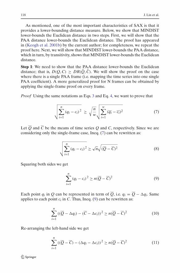
As mentioned, one of the most important characteristics of SAX is that itprovides a lower-bounding distance measure. Below, we show that MINDISTlower-bounds the Euclidean distance in two steps. First, we will show that thePAA distance lower-bounds the Euclidean distance. The proof has appearedin (Keogh et al. 2001b) by the current author; for completeness, we repeat theproof here. Next, we will show that MINDIST lower-bounds the PAA distance,which in turn, by transitivity, shows that MINDIST lower-bounds the Euclideandistance.

Step 1: We need to show that the PAA distance lower-bounds the Euclideandistance; that is, D(Q, C) ≥ DR(Q, C). We will show the proof on the casewhere there is a single PAA frame (i.e. mapping the time series into one singlePAA coefficient). A more generalized proof for N frames can be obtained byapplying the single-frame proof on every frame.

Proof Using the same notations as Eqs. 3 and Eq. 4, we want to prove that

√√√√n∑

i=1

(qi − ci)2 ≥

√nw

√√√√w∑

i=1

(qi − ci)2 (7)

Let Q and C be the means of time series Q and C, respectively. Since we areconsidering only the single-frame case, Ineq. (7) can be rewritten as:

√√√√n∑

i=1

(qi − ci)2 ≥ √

n√

(Q − C)2 (8)

Squaring both sides we get

n∑

i=1

(qi − ci)2 ≥ n(Q − C)2 (9)

Each point qi in Q can be represented in term of Q, i.e. qi = Q − �qi. Sameapplies to each point ci in C. Thus, Ineq. (9) can be rewritten as:

n∑

i=1

((Q − �qi) − (C − �ci))2 ≥ n(Q − C)2 (10)

Re-arranging the left-hand side we get

n∑

i=1

((Q − C) − (�qi − �ci))2 ≥ n(Q − C)2 (11)

Experiencing SAX: a novel symbolic representationof time series 119

We can expand and rewrite Ineq. (11) as:

n∑

i=1

((Q − C)2 − 2(Q − C)(�qi − �ci) + (�qi − �ci)2) ≥ n(Q − C)2

(12)

By distributive law we get:

n∑

i=1

(Q − C)2 −n∑

i=1

2(Q − C)(�qi − �ci) +n∑

i=1

(�qi − �ci)2 ≥ n(Q − C)2

(13)

or

n(Q − C)2 − 2(Q − C)

n∑

i=1

(�qi − �ci) +n∑

i=1

(�qi − �ci)2 ≥ n(Q − C)2

(14)

Recall that qi = Q − �qi, which means that �qi = Q − qi, and similarity,�ci = C − ci. Therefore, the summation part of the second term on the left-hand side of the inequality becomes:

n∑i=1

(�qi − �ci) =n∑

i=1((Q − qi) − (C − ci))

=(

n∑i=1

Q −n∑

i=1qi

)−

(n∑

i=1C −

n∑i=1

ci

)

=((

nQ −n∑

i=1qi

)−

(nC −

n∑i=1

ci

))

=((

n∑i=1

qi −n∑

i=1qi

)−

(n∑

i=1ci −

n∑i=1

ci

))

= 0 − 0= 0

Substituting 0 into the second term on the left-hand side, Ineq. (14) becomes:

n(Q − C)2 − 0 +n∑

i=1

(�qi − �ci)2 ≥ n(Q − C)2 (15)

Cancelling out n(Q − C)2 on both sides of the inequality, we get

120 J. Lin et al.

n∑

i=1

(�qi − �ci)2 ≥ 0 (16)

which always holds true, hence completes the proof.

Step 2: Continuing from Step 1 and using the same methodology, we will nowshow that MINDIST lower-bounds the PAA distance; that is, we will show that

n(Q − C)2 ≥ n(dist(Q, C))2 (17)

Let a = 1, b = 2, and so forth, there are two possible scenarios:

Case 1: |(Q − C)| ≤ 1. In other words, the symbols representing the twotime series are either the same, or consecutive from the alphabet, e.g. Q =C = ‘a’, or Q = ‘a’ and C = ‘b’. From Eq. 6, we know that the MINDIST is 0in this case. Therefore, the right-hand side of Ineq. (17) becomes zero, whichmakes the inequality always hold true.

Case 2: |(Q − C)| > 1. In other words, the symbols representing the two timeseries are at least two alphabets apart, e.g. Q = ‘c’ and C =‘a’. For simplic-ity, assume Q > C; the case where Q < C can be proven in similar fashion.According to Eq. 6, dist(Q, C) is

dist(Q, C) = βQ−1 − βC (18)

For the example above, dist(‘c’,‘a’)= β2 − β1.Recall that Eq. 2 states the following:

ci = alphaj , iif βj−1 ≤ ci < βj

So we know that{

βQ−1 ≤ Q < βQβC−1 ≤ C < βC

(19)

Substituting Eq. 18 into Ineq. (17) we get

n(Q − C)2 ≥ n (βQ−1 − βC)2 (20)

which implies that∣∣∣Q − C

∣∣∣ ≥∣∣∣βQ−1 − βC

∣∣∣ (21)

Note that from our assumptions earlier that |(Q − C)| > 1 and Q > C (i.e. Q isat a “higher” region thanC), we can drop the absolute value notations on bothsides:

Experiencing SAX: a novel symbolic representationof time series 121

Q − C ≥ βQ−1 − βC (22)

Rearranging the terms we get:

Q − βQ−1 ≥ C − βC (23)

which we know always holds true since, from Ineq. (19), we know that

{Q − βQ−1 ≥ 0C − βC < 0

(24)

This completes the proof for Q > C. The case where Q < C can be provensimilarily, and is omitted for brevity.

There is one issue we must address if we are to use a symbolic representationof time series. If we wish to approximate a massive dataset in main memory,the parameters w and a have to be chosen in such a way that the approximationmakes the best use of the primary memory available. There is a clear tradeoffbetween the parameter w controlling the number of approximating elements,and the value a controlling the granularity of each approximating element.

It is unfeasible to determine the best tradeoff analytically, since it is highlydata dependent. We can however empirically determine the best values with asimple experiment. Since we wish to achieve the tightest possible lower bounds,we can simply estimate the lower bounds over all possible feasible parameters,and choose the best settings.

Tightness of Lower Bound = MINDIST(Q, C)

D(Q, C)(25)

We performed such a test with a concatenation of 50 time series datasetstaken from the UCR time series data mining archive. For every combination ofparameters we averaged the result of 100,000 experiments on subsequences oflength 256. Figure 7 shows the results.

The results suggest that using a low value for a results in weak bounds. Whileit’s intuitive that larger alphabet sizes yield better results, there are diminishingreturns as a increases. If space is an issue, an alphabet size in the range 5–8seems to be a good choice that offers a reasonable balance between space andtightness of lower bound—each alphabet within this range can be representedwith just 3 bits. Increasing the alphabet size would require more bits to representeach alphabet.

We end this section with a visual comparison between SAX and the fourmost used representations in the literature (Fig. 8). We can see that SAX pre-serves the general shape of the original time series. Note that since SAX is asymbolic representation, the alphabets can be stored as bits rather than dou-bles, which results in a considerable amount of space-saving. Therefore, SAX

122 J. Lin et al.

23

45

67

8

34

56

78

910

110

0.2

0.4

0.6

0.8

Word Size w Alphabet size a

Ti

thgssen

foe

wol ob r

dnu

Fig. 7 The empirically estimated tightness of lower bounds over the cross product of a = [3. . .11]and w = [2. . .9]. The darker histogram bars illustrate combinations of parameters that requireapproximately equal space to store every possible word

-3-2-10123

DFT

PLA

Haar

APCA

abcdef

Fig. 8 A visual comparison of SAX and the four most common time series data mining representa-tions. A raw time series of length 128 is transformed into the word ffffffeeeddcbaabceedcbaaaaacd-dee. This is a fair comparison since the number of bits in each representation is the same

representation can afford to have higher dimensionality than the other real-val-ued approaches, while using less or the same amount of space.

3.4 Numerosity reduction

We have seen that, given a single time series, our approach can significantlyreduce its dimensionality. In addition, our approach can reduce the numerosityof the data for some applications.

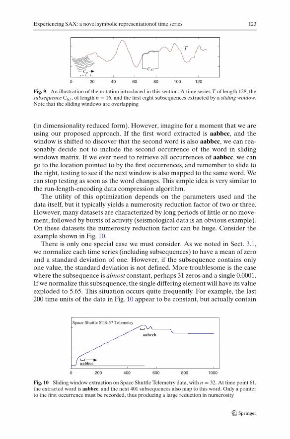
Most applications assume that we have one very long time series T, and thatmanageable subsequences of length n are extracted by use of a sliding window,then stored in a matrix for further manipulation (Chan and Fu 1999; Faloutsoset al. 1994; Keogh et al. 2001a; Yi and Faloutsos 2000). Figure 9 illustrates theidea.

When performing sliding windows subsequence extraction, with any of thereal-valued representations, we must store all |T|−n+1 extracted subsequences

Experiencing SAX: a novel symbolic representationof time series 123

0 20 40 60 80 100 120

T

C 67C pp = 1… 8

Fig. 9 An illustration of the notation introduced in this section: A time series T of length 128, thesubsequence C67, of length n = 16, and the first eight subsequences extracted by a sliding window.Note that the sliding windows are overlapping

(in dimensionality reduced form). However, imagine for a moment that we areusing our proposed approach. If the first word extracted is aabbcc, and thewindow is shifted to discover that the second word is also aabbcc, we can rea-sonably decide not to include the second occurrence of the word in slidingwindows matrix. If we ever need to retrieve all occurrences of aabbcc, we cango to the location pointed to by the first occurrences, and remember to slide tothe right, testing to see if the next window is also mapped to the same word. Wecan stop testing as soon as the word changes. This simple idea is very similar tothe run-length-encoding data compression algorithm.

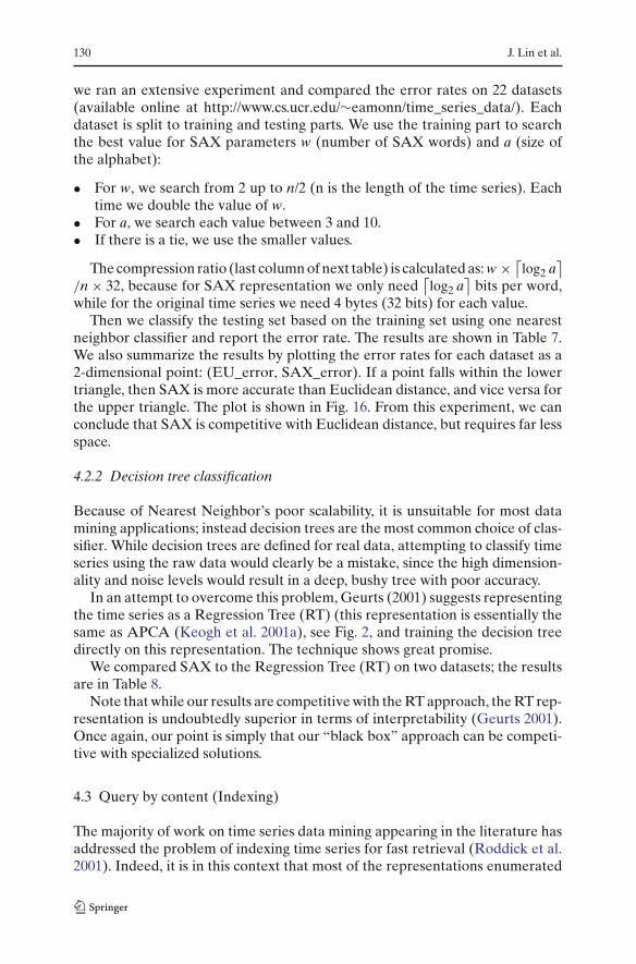
The utility of this optimization depends on the parameters used and thedata itself, but it typically yields a numerosity reduction factor of two or three.However, many datasets are characterized by long periods of little or no move-ment, followed by bursts of activity (seismological data is an obvious example).On these datasets the numerosity reduction factor can be huge. Consider theexample shown in Fig. 10.

There is only one special case we must consider. As we noted in Sect. 3.1,we normalize each time series (including subsequences) to have a mean of zeroand a standard deviation of one. However, if the subsequence contains onlyone value, the standard deviation is not defined. More troublesome is the casewhere the subsequence is almost constant, perhaps 31 zeros and a single 0.0001.If we normalize this subsequence, the single differing element will have its valueexploded to 5.65. This situation occurs quite frequently. For example, the last200 time units of the data in Fig. 10 appear to be constant, but actually contain

0 200 400 600 800 1000

Space Shuttle STS-57 Telemetry

a ccbba

a bccba

Fig. 10 Sliding window extraction on Space Shuttle Telemetry data, with n = 32. At time point 61,the extracted word is aabbcc, and the next 401 subsequences also map to this word. Only a pointerto the first occurrence must be recorded, thus producing a large reduction in numerosity

124 J. Lin et al.

1 2 3 4 5 6 7 8 9 10

S1 S2 S3 S4 S5

1 2 3 4 5 6 7 8 9 10

S1 S2 S3

Contributes to S1with weight 1/3

Contributes to S2with weight 2/3

Contributes to S3with weight 1/3

Contributes to S2with weight 2/3

A

B

Fig. 11 (A) Ten data points are divided into five segments. (B) Ten data points are divided intothree segments. The data points marked with circles contribute to two adjacent segments at thesame time

tiny amounts of noise. If we were to normalize subsequences extracted from thisarea, the normalization would magnify the noise to large meaningless patterns.

We can easily deal with this problem, if the standard deviation of the sequencebefore normalization is below an epsilon ε, we simply assign the entire word tothe middle-ranged alphabet (e.g. cccccc if a = 5).

3.5 Relaxation on the number of segments

So far we have described SAX with the assumption that the length of the timeseries is divisible by the number of segments, i.e. n/w must be an integer. If nis not dividable by w, there will be some points in the time series that we arenot sure which segment to put them. For example, in Fig. 11A, we are dividing10 data points into five segments. And it is obvious that point 1, 2 should be insegment 1; point 3, 4 should be in segment 2; so on and so forth. In in Fig. 11B,we are dividing 10 data points into three segments. It’s not clear which segmentpoint 4 should go: segment 1 or segment 2. Same problem holds for point 7.The assumption n must be dividable by w clearly limits our choices of w, andis problematic if n is a prime number. Here we show that this needs not be thecase and provide a simple solution when n is not divisible by w.

Instead of putting the whole point into a segment, we can put part of it. Forexample, in in Fig. 11B, point 4 contributes its 1/3 to segment 1 and its 2/3 tosegment 2, and point 7 contributes its 2/3 to segment 2 and its 1/3 to segment 3.This makes each segment contains exactly 3 1/3 data points and solves the un-dividable problem. This generalization is implemented in the later version ofSAX, as well as some of the applications that utilize SAX.

4 Experimental validation of our symbolic approach

In this section, we perform various data mining tasks using our symbolicapproach and compare the results with other well-known existing approaches.

Experiencing SAX: a novel symbolic representationof time series 125

For clustering, classification, and anomaly detection, we compare the resultswith the classic Euclidean distance, and with other previously proposed sym-bolic approaches. Note that none of these other approaches use dimensionalityreduction. In the next paragraphs we summarize the strawmen representationsthat we compare ours to. We choose these two approaches since they are typicalrepresentatives of approaches in the literature.

André-Jönsson, and Badal (1997) proposed the SDA algorithm that com-putes the changes between values from one instance to the next, and dividethe range into user-predefined sections. The disadvantages of this approach areobvious: prior knowledge of the data distribution of the time series is requiredin order to set the breakpoints; and the discretized time series does not conservethe general shape or distribution of the data values.

Huang and Yu proposed the IMPACTS algorithm, which uses change ratiobetween one time point to the next time point to discretize the time series(Huang and Yu 1999). The range of change ratios are then divided into equal-sized sections and mapped into symbols. The time series is converted to adiscretized collection of change ratios. As with SAX, the user needs to definethe cardinality of symbols.

4.1 Clustering

Clustering is one of the most common data mining tasks, being useful in its ownright as an exploratory tool, and also as a sub-routine in more complex algo-rithms (Ding et al. 2002; Fayyad et al. 1998; Kalpakis et al. 2001). We considertwo clustering algorithms, one of hierarchical clustering, and one of partitionalclustering.

4.1.1 Hierarchical clustering

Comparing hierarchical clusterings is a very good way to compare and contrastsimilarity measures, since a dendrogram of size N summarizes O(N2) distancecalculations (Keogh and Kasetty 2002). The evaluation is typically subjective,we simply adjudge which distance measure appears to create the most naturalgroupings of the data. However, if we know the data labels in advance we canalso make objective statements of the quality of the clustering. In Fig. 12 weclustered nine time series from the Control Chart dataset, three each from thedecreasing trend, upward shift and normal classes.

In this case we can objectively state that SAX is superior, since it correctlyassigns each class to its own subtree. This is simply a side effect due to thesmoothing effect of dimensionality reduction. Therefore, it’s not surprising thatSAX can sometimes outperform the simple Euclidean distance, especially onnoisy data, or data with shifting on the time-axis. This fact is demonstrated inthe dendrogram produced by Euclidean distance: the “normal” class, whichcontains a lot of noise, is not clustered correctly. More generally, we observedthat SAX closely mimics Euclidean distance on various datasets.

126 J. Lin et al.

Euclidean

IMPACTS (alphabet=8) SDA

SAX

Fig. 12 A comparison of the four distance measures’ ability to cluster members of the ControlChart dataset. Complete linkage was used as the agglomeration technique

The reasons that SDA and IMPACTS perform poorly, we observe, are thatneither symbolic representation is very descriptive of the general shape of thetime series, and that the lack of dimensionality reduction can further distort theresults if the data is noisy. What SDA does is essentially differencing the timeseries, and then discretizing the resulting series. While differencing has beenused historically in statistical time series analysis, its purposes to remove someautocorrelation, and to make a time series stationary are not always applicablein determination of similarity in data mining. In addition, although computingthe derivatives tells the type of change from one time point to the next timepoint: sharp increase, slight increase, sharp decrease, etc., this approach doesn’tappear very useful since time series data are typically noisy. More specifically,in addition to the overall trends or shapes, there are noises that appear through-out the entire time series. Without any smoothing or dimensionality reduction,these noises are likely to overshadow the actual characteristics of the time series.

To demonstrate why the “decreasing trend” and the “upward shift” classesare indistinguishable by the clustering algorithm for SDA, let’s look at what thedifferenced series look like. Figure 13 shows the original time series and theircorresponding series after differencing. It’s clear that the differenced seriesfrom the same class are not any more similar than those from a different class.As a matter of fact, as we compute the pairwise distances between all 6 differ-enced series, we realize that the distances are not indicative at all of the classesthese data belong. Table 5 and Table 6 show the inter- and the intra-distancesbetween the series (the series from the “decreasing trend” class are denoted asAi, and the series from the “upward shift” are denoted as Bi).

Experiencing SAX: a novel symbolic representationof time series 127

Fig. 13 (A) Time series from the “decreasing trend” class and the resulting series after differencing.(B) Time series from the “upward shift” class and the resulting series after differencing

Table 5 Intra-class distancesbetween the differenced timeseries from the “decreasingtrend” class

A1 A2 A3

A1 0 60.59 59.08A2 60.59 0 57.12A3 59.08 57.12 0

Table 6 Inter-class distancesbetween the differenced timeseries from the “decreasingtrend” and the “upward shift”classes

B1 B2 B3

A1 49.92 46.02 49.21A2 54.24 58.07 61.38A3 51.28 49.07 51.72

Interestingly, in Gavrilov et al. (2000), the authors show that taking the firstderivatives (i.e. differencing) actually worsens the results when compared tousing the raw data. Our experimental results validate their observations.

IMPACTS suffers from similar problems as SDA. In addition, it’s clear thatneither IMPACTS nor SDA can beat simple Euclidean distance, and the discus-sion above applies to all data mining tasks, since the problems lie in the natureof the representations.

4.1.2 Partitional clustering

Although hierarchical clustering is a good sanity check for any proposed dis-tance measure, it has limited utility for data mining because of its poor scala-bility. The most commonly used data mining clustering algorithm is k-means(Fayyad et al. 1998), so for completeness we will consider it here. We performedk-means on both the original raw data, and our symbolic representation. Fig-ure 14 shows a typical run of k-means on a space telemetry dataset. Both algo-rithms converge after 11 iterations. Since k-means algorithm seeks to optimizethe objective function, by minimizing the sum of squared intra-cluster error,

128 J. Lin et al.

we compare and plot the objective functions, after projecting the data backto its original dimension (for fair comparison of objective functions), for eachiteration. The objective function for a given clustering is given by Eq. 26, wherexi is the time series, and cm is the cluster center of the cluster that xi belongsto. The smaller the objective function, the more compact (thus better) theclusters.

F =k∑

m=1

N∑

i=1

‖xi − cm‖ (26)

The results here are quite unintuitive and surprising: working with an approx-imation of the data gives better results than working with the original data.Fortunately, a recent paper offers a suggestion as to why this might be so. It hasbeen shown that initializing the clusters centers on a low dimension approxima-tion of the data can improve the quality (Ding et al. 2002), this is what clusteringwith SAX implicitly does.

In Section 4.4.3 we introduce another distance measure based on SAX. Byapplying it on clustering, we show that it outperforms the Euclidean distancemeasure.

4.2 Classification

Classification of time series has attracted much interest from the data miningcommunity. Although special- purpose algorithms have been proposed (Keoghand Pazzani 1998), we will consider only the two most common classificationalgorithms for brevity, clarity of presentations and to facilitate independentconfirmation of our findings.

4.2.1 Nearest neighbor classification

To compare different distance measures on 1-nearest-neighbor classification,we use leaving-one-out cross validation. Firstly, we compare SAX with Euclid-ean distance, IMPACTS, SDA, and LPinf . Two classic synthetic datasets areused: the Cylinder-Bell-Funnel (CBF) dataset has 50 instances of time seriesfor each of the three clusters, and the Control Chart (CC) has 100 instances foreach of the six clusters (Keogh and Kasetty 2002).

Since SAX allows dimensionality and alphabet size as user input, and theIMPACTS allows variable alphabet size, we ran the experiments on differ-ent combinations of dimensionality reduction and alphabet size. For the otherapproaches we applied the simple dimensionality reduction technique of skip-ping data points at a fixed interval. In Fig. 15, we show the result with a dimen-sionality reduction of 4 to 1.

Experiencing SAX: a novel symbolic representationof time series 129

Number of Iterations

220000

225000

230000

235000

240000

245000

250000

255000

260000

265000

1 2 3 4 5 6 7 8 9 10 11

Obj

ectiv

e Fu

nctio

n

Raw data

SAX

Fig. 14 A comparison of the k-means clustering algorithm using SAX and using the raw data. Thedataset was Space Shuttle telemetry, 1,000 subsequences of length 512. Surprisingly, working withthe symbolic approximation produces better results than working with the original data

5 7 8 9 10

Impacts

SDA

Euclidean

LPmax

SAX

0

0.1

0.2

0.3

0.4

0.5

0.6

5 7 8 9 10

Control ChartCylinder -Bell -Funnel

Err

or R

ate

Alphabet Size Alphabet Size

6 6

Fig. 15 A comparison of five distance measures utility for nearest neighbor classification. Wetested different alphabet sizes for SAX and IMPACTS, SDA’s alphabet size is fixed at 5

Similar results were observed for other levels of dimensionality reduction.Once again, SAX’s ability to beat Euclidean distance is probably due to thesmoothing effect of dimensionality reduction, nevertheless this experiment doesshow the superiority of SAX over the others proposed in the literature.

Since both IMPACTS and SDA perform poorly compared to Euclidean dis-tance and SAX, we will exclude them from the rest of the classification experi-ments. To provide a closer look on how SAX compares to Euclidean distance,

130 J. Lin et al.

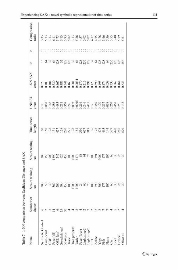
we ran an extensive experiment and compared the error rates on 22 datasets(available online at http://www.cs.ucr.edu/∼eamonn/time_series_data/). Eachdataset is split to training and testing parts. We use the training part to searchthe best value for SAX parameters w (number of SAX words) and a (size ofthe alphabet):

• For w, we search from 2 up to n/2 (n is the length of the time series). Eachtime we double the value of w.

• For a, we search each value between 3 and 10.• If there is a tie, we use the smaller values.

The compression ratio (last column of next table) is calculated as: w × ⌈log2 a

⌉

/n × 32, because for SAX representation we only need⌈

log2 a⌉

bits per word,while for the original time series we need 4 bytes (32 bits) for each value.

Then we classify the testing set based on the training set using one nearestneighbor classifier and report the error rate. The results are shown in Table 7.We also summarize the results by plotting the error rates for each dataset as a2-dimensional point: (EU_error, SAX_error). If a point falls within the lowertriangle, then SAX is more accurate than Euclidean distance, and vice versa forthe upper triangle. The plot is shown in Fig. 16. From this experiment, we canconclude that SAX is competitive with Euclidean distance, but requires far lessspace.

4.2.2 Decision tree classification

Because of Nearest Neighbor’s poor scalability, it is unsuitable for most datamining applications; instead decision trees are the most common choice of clas-sifier. While decision trees are defined for real data, attempting to classify timeseries using the raw data would clearly be a mistake, since the high dimension-ality and noise levels would result in a deep, bushy tree with poor accuracy.

In an attempt to overcome this problem, Geurts (2001) suggests representingthe time series as a Regression Tree (RT) (this representation is essentially thesame as APCA (Keogh et al. 2001a), see Fig. 2, and training the decision treedirectly on this representation. The technique shows great promise.

We compared SAX to the Regression Tree (RT) on two datasets; the resultsare in Table 8.

Note that while our results are competitive with the RT approach, the RT rep-resentation is undoubtedly superior in terms of interpretability (Geurts 2001).Once again, our point is simply that our “black box” approach can be competi-tive with specialized solutions.

4.3 Query by content (Indexing)

The majority of work on time series data mining appearing in the literature hasaddressed the problem of indexing time series for fast retrieval (Roddick et al.2001). Indeed, it is in this context that most of the representations enumerated

Experiencing SAX: a novel symbolic representationof time series 131

Tabl

e7

1-N

Nco

mpa

riso

nbe

twee

nE

uclid

ean

Dis

tanc

ean

dSA

X

Nam

eN

umbe

rof

Size

oftr

aini

ngSi

zeof

test

ing

Tim

ese

ries

1-N

NE

U1-

NN

SAX

wa

Com

pres

sion

clas

ses

set

set

leng

ther

ror

erro

rra

tio

Synt

heti

cC

ontr

ol6

300

300

600.

120.

0216

103.

33G

un-p

oint

250

150

150

0.08

70.

1864

105.

33C

BF

330

900

128

0.14

80.

104

3210

3.13

Face

(all)

1456

016

9013

10.

286

0.33

064

106.

11O

SUle

af6

200

242

427

0.48

30.

467

128

103.

75Sw

edis

hle

af15

500

625

128

0.21

10.

483

3210

3.13

50W

ords

5045

045

527

00.

369

0.34

112

810

5.93

Trac

e4

100

100

275

0.24

0.46

128

105.

82Tw

opa

tter

ns4

1000

4000

128

0.09

30.

081

3210

3.13

Waf

er2

1000

6174

152

0.00

450.

0034

6410

5.26

Face

(fou

r)4

2488

350

0.21

60.

170

128

104.

57L

ight

ning

-22

6061

637

0.24

60.

213

256

105.

02L

ight

ning

-77

7073

319

0.42

50.

397

128

105.

02E

CG

210

010

096

0.12

0.12

3210

4.17

Adi

ac37

390

391

176

0.38

90.

890

6410

4.55

Yog

a2

300

3000

426

0.17

00.

195

128

103.

76Fi

sh7

175

175

463

0.21

70.

474

128

103.

46P

lane

710

510

514

40.

038

0.03

864

105.

56C

ar4

6060

577

0.26

70.

333

256

105.

55B

eef

530

3047

00.

467

0.56

712

810

3.40

Cof

fee

228

2828

60.

250.

464

128

105.

59O

live

oil

430

3057

00.

133

0.83

325

610

5.61

132 J. Lin et al.

0 0.1 0.2 0.3 0.4 0.5 0.6 0.7 0.8 0.9 10

0.1

0.2

0.3

0.4

0.5

0.6

0.7

0.8

0.9

1

Error Rate of Euclidean Distance

rE

orr

aR

eto

fAS

Xe

R pr

seatne

oitn

In this regionSAX representationis more accurate

In this regionEuclidean distanceis more accurate

Fig. 16 Error rates for SAX and Euclidean distance on 22 datasets. Lower triangle is the regionwhere SAX is more accurate than Euclidean distance, and upper triangle is where Euclideandistance is more accurate than SAX

in Fig. 1 were introduced (Chan and Fu 1999; Faloutsos et al. 1994; Keogh et al.2001a; Yi and Faloutsos 2000). Dozens of papers have introduced techniques todo indexing with a symbolic approach (Andre-Jonsson and Badal 1997; Huangand Yu 1999), but without exception, the answer set retrieved by these tech-niques can be very different to the answer set that would be retrieved by thetrue Euclidean distance. It is only by using a lower bounding technique that onecan guarantee retrieving the full answer set, with no false dismissals (Faloutsoset al. 1994).

To perform query by content, we build an index using SAX, and compare itto an index built using the Haar wavelet approach (Chan and Fu 1999). Sincethe datasets we use are large and disk-resident, and the reduced dimensionalitycould still be potentially high (or at least high enough such that the performancedegenerates to sequential scan if R-tree were used (Hellerstein et al. 1997)),we use Vector Approximation (VA) file as our indexing algorithm. We note,however, that SAX could also be indexed by classic string indexing techniquessuch as suffix trees.

Table 8 A comparison of SAX with the specialized Regression Tree approach for decision treeclassification

Dataset SAX Regression Tree

CC 3.04 ± 1.64 2.78 ± 2.11CBF 0.97 ± 1.41 1.14 ± 1.02

Our approach used an alphabet size of 6, both approaches used a dimensionality of 8

Experiencing SAX: a novel symbolic representationof time series 133

0

0.1

0.2

0.3

0.4

0.5

0.6

Ballbeam Chaotic Memory Winding

Dataset

DWT Haar

SAX

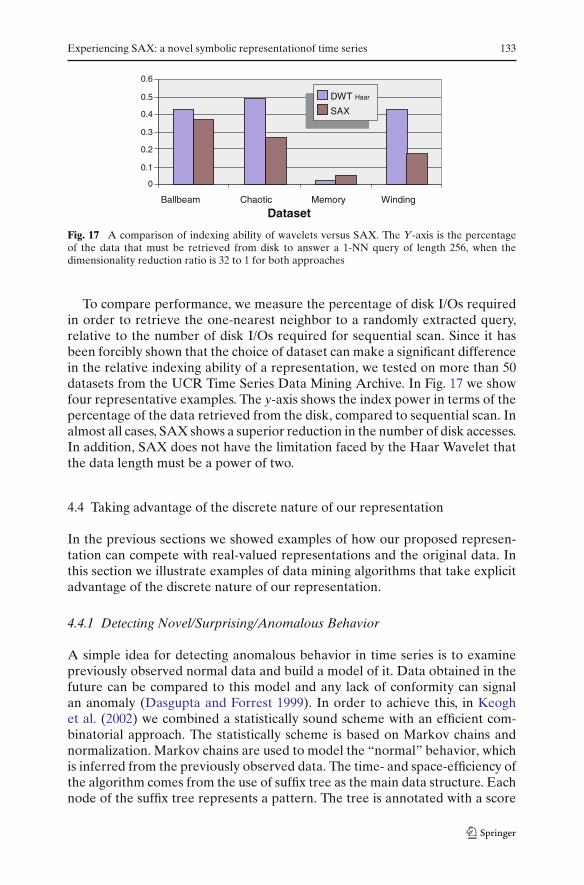
Fig. 17 A comparison of indexing ability of wavelets versus SAX. The Y-axis is the percentageof the data that must be retrieved from disk to answer a 1-NN query of length 256, when thedimensionality reduction ratio is 32 to 1 for both approaches

To compare performance, we measure the percentage of disk I/Os requiredin order to retrieve the one-nearest neighbor to a randomly extracted query,relative to the number of disk I/Os required for sequential scan. Since it hasbeen forcibly shown that the choice of dataset can make a significant differencein the relative indexing ability of a representation, we tested on more than 50datasets from the UCR Time Series Data Mining Archive. In Fig. 17 we showfour representative examples. The y-axis shows the index power in terms of thepercentage of the data retrieved from the disk, compared to sequential scan. Inalmost all cases, SAX shows a superior reduction in the number of disk accesses.In addition, SAX does not have the limitation faced by the Haar Wavelet thatthe data length must be a power of two.

4.4 Taking advantage of the discrete nature of our representation

In the previous sections we showed examples of how our proposed represen-tation can compete with real-valued representations and the original data. Inthis section we illustrate examples of data mining algorithms that take explicitadvantage of the discrete nature of our representation.

4.4.1 Detecting Novel/Surprising/Anomalous Behavior

A simple idea for detecting anomalous behavior in time series is to examinepreviously observed normal data and build a model of it. Data obtained in thefuture can be compared to this model and any lack of conformity can signalan anomaly (Dasgupta and Forrest 1999). In order to achieve this, in Keoghet al. (2002) we combined a statistically sound scheme with an efficient com-binatorial approach. The statistically scheme is based on Markov chains andnormalization. Markov chains are used to model the “normal” behavior, whichis inferred from the previously observed data. The time- and space-efficiency ofthe algorithm comes from the use of suffix tree as the main data structure. Eachnode of the suffix tree represents a pattern. The tree is annotated with a score

134 J. Lin et al.

I)

-5

0

5

0 100 200 300 400 500 600 700 800 900 1000-5

0

5

0 100 200 300 400 500 600 700 800 900 1000

II)

III)

IIII)

V)

VI)

VII)

Fig. 18 A comparison of five anomaly detection algorithms on the same task. (I) The trainingdata, a slightly noisy sine wave of length 1,000. (II) The time series to be examined for anomaliesis a noisy sine wave that was created with the same parameters as the training sequence, then anassortment of anomalies were introduced at time periods 250, 500 and 750. (III) and (IIII) TheMarkov model technique using the IMPACTS and SDA representations did not clearly discoverthe anomalies, and reported some false alarms. (V) The IMM anomaly detection algorithm appearsto have discovered the first anomaly, but it also reported many false alarms. (VI) The TSA-Treeapproach is unable to detect the anomalies. (VII) The Markov model-based technique using SAXclearly finds the anomalies, with no false alarms

obtained comparing the support of a pattern observed in the new data with thesupport recorded in the Markov model. This apparently simple strategy turnsout to be very effective in discovering surprising patterns. In the original workwe use a simple symbolic approach, similar to IMPACTS (Huang and Yu 1999);here we revisit the work using SAX.

For completeness, we will compare SAX to two highly referenced anomalydetection algorithms that are defined on real valued representations, the TSA-tree Wavelet based approach of Shahabi et al. (2000) and the Immunology(IMM) inspired work of Dasgupta and Forrest (1999). We also include the Mar-kov technique using IMPACTS and SDA in order to discover how much of thedifference can be attributed directly to the representation. Figure 18 containsan experiment comparing all five techniques.

The results on this simple experiment are impressive. Since suffix trees andMarkov models can be used only on discrete data, this offers a motivationfor our symbolic approach. While all the other approaches, including the Mar-kov Models using IMPACTS and SDA representations, the Immunology-basedanomaly detection approach, and the TSA-Tree approach, did not clearly dis-cover the anomalies and reported some false alarms, the SAX-based MarkovModel clearly finds the anomalies with no false alarms.

4.4.2 Motif discovery

It is well understood in bioinformatics that overrepresented DNA sequencesoften have biological significance (Apostolico et al. 2002; Durbin et al. 1998;

Experiencing SAX: a novel symbolic representationof time series 135

0 500 1000 1500 2000 2500

0 20 40 60 80 100 120

BAWinding Dataset (Angular speed of reel 1)

A

B

Fig. 19 Above, a motif discovered in a complex dataset by the modified Projection algorithm.Below, the motif is best visualized by aligning the two subsequences and “zooming in”. The similarityof the two subsequences is striking, and hints at unexpected regularity

Reinert et al. 2000). A substantial body of literature has been devoted to tech-niques to discover such patterns (Gionis and Mannila 2003; Staden et al. 1989;Tompa and Buhler 2001). In a previous work, we defined the related concept of“time series motif” (Lin et al. 2002). Time series motifs are close analogues oftheir discrete cousins, although the definitions must be augmented to preventcertain degenerate solutions. The naïve algorithm to discover the motifs is qua-dratic in the length of the time series. In Lin et al. (2002), we demonstrated asimple technique to mitigate the quadratic complexity by a large constant factor,nevertheless this time complexity is clearly untenable for most real datasets.

The symbolic nature of SAX offers a unique opportunity to avail of thewealth of bioinformatics research in this area. In particular, recent work byTompa and Buhler holds great promise (Tompa and Buhler 2001). The authorsshow that many previously unsolvable motif discovery problems can be solvedby hashing subsequences into buckets using a random subset of their featuresas a key, then doing some post-processing search on the hash buckets.3 Theycall their algorithm Projection.

We carefully reimplemented the random projection algorithm of Tompa andBuhler, making minor changes in the post-processing step to allow for the factthat although we are hashing random projections of our symbolic representa-tion, we actually wish to discover motifs defined on the original raw data (Chiuet al. 2003). Figure 19 shows an example of a motif discovered in an indus-trial dataset (Bastogne et al. 2002) using this technique. The patterns found areextremely similar to one another.

Apart from the attractive scalability of the algorithm, there is another impor-tant advantage over other approaches. The Projection algorithm is able todiscover motifs even in the presence of noise. Our extension of the algorithm

3 Of course, this description greatly understates the contributions of this work. We urge the readerto consult the original paper.

136 J. Lin et al.

inherits this robustness to noise. We direct interested readers to Chiu et al.(2003) for more detailed discussion of this algorithm.

4.4.3 Visualization

Data visualization techniques are very important for data analysis, since thehuman eye has been frequently advocated as the ultimate data-mining tool.However, despite their illustrative nature, which can provide users better under-standing of the data and intuitive interpretation of the mining results, there hasbeen surprisingly little work on visualizing large time series datasets. One reasonfor this lack of interest is that time series data are also usually very massive insize. With limited pixel space and the typically enormous amount of data athand, it is infeasible to display all the data on the screen at once, much less find-ing any useful information from the data. How to efficiently organize the dataand present them in such a way that is intuitive and comprehensible to humaneyes thus remains a great challenge. Ideally, the visualization technique shouldfollow the Visual Information Seeking Mantras, as summarized by Dr. BenShneiderman: “Overview, zoom & filter, details-on-demand.” In other words,it should be able to provide users the overview or summary of the data, andallows users to further investigate on the interesting patterns highlighted by thetool. To this end, we developed VizTree (Lin et al. 2004), a time series patterndiscovery and visualization system based on augmenting suffix trees. VizTreevisually summarizes both the global and local structures of time series dataat the same time. In addition, it provides novel interactive solutions to manypattern discovery problems, including the discovery of frequently occurringpatterns (motif discovery), surprising patterns (anomaly detection), and queryby content. The user interactive paradigm allows users to visually explore thetime series, and perform real-time hypotheses testing. Since the use of suffixtree requires that the input data be discrete, SAX is the perfect candidate fordiscretizing the time series data.

Compared to the existing time series visualization systems in the literature,VizTree is unique in several respects. First, almost all other approaches assumehighly periodic time series, whereas VizTree makes no such assumption. Othermethods typically require space (both memory space, and pixel space) thatgrows at least linearly with the length of the time series, making them untena-ble for mining massive datasets. Finally, VizTree allows us to visualize a muchricher set of features, including global summaries of the differences betweentwo time series, locally repeated patterns, anomalies, etc.

In VizTree, patterns are represented in a depth-limited tree structure, inwhich their frequencies of occurrence are encoded in the thicknesses of branches.The algorithm works by sliding a window across the time series and extractingsubsequences of user-defined lengths. The subsequences are then discretizedinto strings by SAX and inserted into an augmented suffix tree. Each string isregarded as a pattern, and the frequency of occurrence for each pattern is en-coded by the thickness of the branch: the thicker the branch, the more frequentthe corresponding pattern. Motif discovery and anomaly detection can thus be

Experiencing SAX: a novel symbolic representationof time series 137

Fig. 20 Anomaly detection on power consumption data. The anomaly shown here is a short weekduring Christmas

easily achieved: those that occur frequently can be regarded as motifs, and thosethat occur rarely can be regarded as anomaly. Figure 20 shows the screenshot ofVizTree for anomaly detection on the Dutch power demand dataset. Electricityconsumption is recorded every 15 min; therefore, for the year of 1997, there are35,040 data points. The majority of the weeks follow the regular Monday-Fri-day, 5-working-day pattern, as shown by the thick branches. The thin branchesdenote the anomalies (in the sense that the electricity consumption is abnor-mal given the day of the week). Note that in VizTree, we reverse the alphabetordering so the alphabets now read top-down rather than bottom-up (e.g. ‘a’ isnow in the topmost branch, rather than in the bottom-most branch). This way,the string better describes the actual shape of the time series—‘a’ denotes thetop region, ‘b’ the middle region, ‘c’ the bottom region. The top right windowshows the subtree when we click on the 2nd child of the root node. Clickingon any of the existing branches (in the main or the subtree window) will plotthe subsequences represented by them in the bottom right window. The high-lighted, circled subsequence is retrieved by clicking on the branch “bab.” Thezoom-in shows why it is an anomaly: it’s the beginning of the three-day weekduring Christmas (Thursday and Friday off). The other thin branches denoteother anomalies such as New Year’s Day, Good Friday, Queen’s Birthday, etc.

The evaluation for visualization techniques is usually subjective. AlthoughVizTree clearly demonstrates its capability in detecting non-trivial patterns, inLin et al. (2005) we also devise a measure that quantifies the effectiveness of the

138 J. Lin et al.

Fig. 21 Clustering result using the (dis)similarity coefficient

algorithm. The measure, which we call the “dissimilarity coefficient,” describeshow dissimilar two time series are, and ranges from 0 to 1. In essence, the coeffi-cient summarizes the difference in “behavior” of each pattern (represented bya string) in two time series. More concretely, for each pattern, we count itsrespective numbers of occurrences in both time series, and see how much thefrequencies differ. We call this measure support, which is then weighted by theconfidence, or the degree of “interestingness” of the pattern. For example, apattern that occurs 120 times in time series A and 100 times in time series B isprobably less significant than a pattern that occurs 20 times in A but zero timesin B, even though the support for both cases is 20.

Subtracting the dissimilarity coefficient from 1 then gives us a novel simi-larity measure that describes how similar two time series are. More details onthe (dis)similarity measure can be found in Lin et al. (2005). An important factabout this similarity measure is that, unlike a distance measure that computespoint-to-point distances, it captures the global structure of the time series ratherthan local differences. This time-invariant feature is useful if we are interestedin the overall structures of the time series. Figure 21 shows the dendrogram ofclustering result using the (dis)similarity coefficient as the distance measure. Itclearly demonstrates that the coefficient captures the dissimilarity very well andthat all clusters are separated perfectly. Note that it’s even able to distinguishthe four different sets of heartbeats (from top down, clusters 1, 4, 5, and 6)!

As a reference, we ran the same clustering algorithm using the widely-usedEuclidean distance. The result is shown in Fig. 22. Clearly, clustering using our(dis)similarity measure returns superior results.

So far we discussed how the symbolic nature of SAX makes possible theapproaches that were not considered, at least not effectively, by the time series

Experiencing SAX: a novel symbolic representationof time series 139

Fig. 22 Clustering result using Euclidean distance

data mining community before, since these approaches require the input bediscrete. It sheds some light in offering efficient solutions on various problemsfrom a new direction. The problems listed in this section, however, are just asmall subset of examples that show the efficacy of SAX. We have since thenproposed more algorithms on anomaly detection (HOT SAX) (Keogh et al.2005), contrast sets mining (Lin and Keogh 2006), visualization by time seriesbitmaps (Kumar et al. 2005), clustering (Ratanamahatana et al. 2005), com-pression-based distance measures (Keogh et al. 2004), etc., all of which basedon SAX. In the next section, we discuss the evident impact of SAX, illustratedby great interests from other researchers/users from both the academic and theindustrial communities.

4.5 The impact of SAX

In the relatively short time since its initial introduction, SAX has had a largeimpact in industry and academia. Below we summarize some of this work, with-out attempting to be exhaustive. We can broadly classify this work into thosewho have simply used the original formulation of SAX to solve a particular prob-lem, and those who have attempted to extend or augment SAX in some way.

4.5.1 Applications of SAX

In addition to the applications mentioned in this section, it has been usedworldwide in various domains. To name a few, in Androulakis (2005) the au-thors analyzed complex kinetic mechanisms using a method based on SAX.

140 J. Lin et al.

In Ferreira (2006) the authors consider the problem of analysis of proteinunfolding data. After noting that “a complexity/dimensionality reduction on thedata may be necessary and desirable” the authors consider various alternativesbefore noting “We adopted a two step approach called SAX .” Dr. Amy McGov-ern of the University of Oklahoma is leading a project on dynamic relationalmodels for improved hazardous weather prediction. In attempting to use prop-ositional models for this task, her group needs a discrete representation of thereal-valued metrological data, and they noted in a recent paper “We are cur-rently using (Lin et al.’s SAX approach to creating discrete data from continuousdata”(McGovern et al. 2006). In Duchene and Garbay (2005), Duchene et al.(2004), Silvent et al. (2003, 2004), the authors use SAX and random projec-tion to discover motifs in telemedicine time series. In Chen et al. (2005) theauthors convert palmprint to time series, then to SAX, then they do biometricrecognition. The authors in Tanaka and Uehara (2004) use SAX and randomprojection to mine motion capture data. In Celly and Zordan (2004) SAX isused to find repeated patterns in motion capture data. Ohsaki et al. (2003) usesSAX to find rules in time series. In Tanaka and Uehara (2003) the authors useSAX to find motifs of unspecified length. In Murakami et al. (2004) SAX isused to find repeated patterns in robot sensors. In Bakalov et al. (2005), theauthors use SAX to do spatiotemporal trajectory joins. In Pouget et al. (2006)the authors use SAX to “detect multi-headed stealthy attack tools”.

4.5.2 Extensions to SAX

As noted above, there have been dozens of applications of SAX to diverseproblems. However, there has been surprisingly little work to augment or ex-tend the SAX representation itself. We attribute this to the generality of theoriginal framework; it simply works very well for most problems. Nevertheless,recently there have been some SAX extensions, which we consider below.

In Lkhagva et al. (2006) the authors augment each SAX symbol by incorpo-rating the minimum and maximum value in the range. Thus each SAX segmentcontains a triplet of information, rather that a single symbol. Very preliminaryresults are presented which suggest that this may be useful in some domains.Hugueney (2006) (2001b) has recently suggested that SAX could be improvedby allowing SAX symbols to adaptively represent different length sections of atime series. Just as SAX may be seen as symbolic a symbolic version of the PAArepresentation (Keogh et al. 2001b), Dr. Hugueneys approach may be seen assymbolic a symbolic version of the APCA representation (Keogh et al. 2001a).While the author shows that this does decrease the reconstruction error on somedatasets, it is not obvious that the new representation can be used with hashing(as in Lin et al. (2002)) or with suffix trees (as in Lin et al. (2004)). In contrastto Hugueneys idea of allowing segment lengths to be adaptive, recent work byMörchen and Ultsch has suggested that the breakpoints should be adaptive(Mörchen and Ultsch 2005). The authors make a convincing case that in somedatasets this may be better than the Gaussian assumption (cf. Section 3.2).For example they consider a time series of muscle activity and show that it

Experiencing SAX: a novel symbolic representationof time series 141

strongly violates the Gaussian assumption. Note that once the new breakpointsare defined, and Tables 3 and 4 are appropriately adjusted, the lower boundingproperty still holds. Finally, in an interesting new development, Wei et al (2006)have shown techniques to adapt SAX to various problems in 2D shape match-ing, after modifying algorithms/representations to allow for rotation invariance,which in the SAX representation corresponds to circular shifts.

The list of papers using SAX keeps growing at rapid rate. The wide accep-tance of SAX by fellow researchers has shown its generality and utilities indiverse domains. There is great potential for adapting and extending SAX onan even broader class of data mining problems.

5 Conclusions and future directions

In this work we have formulated the first dimensionality/numerosity reduction,lower bounding symbolic approach in the literature. We have shown that ourrepresentation is competitive with, or superior to, other representations on awide variety of classic data mining problems, and that its discrete nature allowsus to tackle emerging tasks such as anomaly detection, motif discovery andvisualization.

A host of future directions suggest themselves. There is an enormous wealthof useful definitions, algorithms and data structures in the bioinformatics lit-erature that can be exploited by our representation (Apostolico et al. 2002;Durbin et al. 1998; Gionis and Mannila 2003; Lonardi et al. 2001; Reinert et al.2000; Staden et al. 1989; Tompa and Buhler 2001). It may be possible to create alower bounding approximation of Dynamic Time Warping (Berndt and Clifford1994), by slightly modifying the classic string edit distance. Finally, there maybe utility in extending our work to multidimensional and streaming time series(Vlachos et al. 2002).

References

Agrawal R, Psaila G, Wimmers EL, Zait M (1995) Querying shapes of histories. In: Proceedingsof the 21st International conference on very large databases, Zurich, Switzerland, Sept 11–15,pp 502–514

Andre-Jonsson H, Badal D (1997) Using signature files for querying time-series data (1997) In:Proceedings of principles of data mining and knowledge discovery, 1st European symposium,Trondheim, Norway. June 24–27, pp 211–220

Androulakis IP (2005) New approaches for representing, analyzing and visualizing complex kineticmechanisms. In: Proceedings of the 15th European symposium on computer aided processengineering, Barcelona, Spain. May 29–June 1

Apostolico A, Bock ME, Lonardi S (2002) Monotony of surprise in large-scale quest for unusualwords. In: Proceedings of the 6th International conference on research in computationalmolecular biology, Washington, DC, April 18–21, pp 22–31

Bagnall AJ, Janakec G (2004) Clustering time series from arma models with clipped data. In:Proceedings of the 10th ACM SIGKDD International conference on knowledge discoveryand data mining, Seattle, WA. August 22–25, pp 49–58

142 J. Lin et al.

Bakalov P, Hadjieleftherious M, Tsotras VJ (2005) Time relaxed spatiotemporal trajectory. In:Proceedings of the ACM international symposium on advances in geographic informationsystems, Bremen, Germany. November 4–5

Bastogne T, Noura H, Richard A, Hittinger JM (2002) Application of subspace methods to theidentification of a winding process. In: Proceedings of the 4th European control conference,Brussels, Belgium

Berndt D, Clifford J (1994) Using dynamic time warping to find patterns in time series, Theworkshop on knowledge discovery in databases, the 12th International conference on artificialintelligence, Seattle, WA, pp 229–248

Celly B, Zordan VB (2004) Animated people textures. In: Proceedings of the 17th internationalconference on computer animation and social agents, Geneva, Switzerland, July 7–9

Chan K, Fu AW (1999) Efficient time series matching by wavelets. In: Proceedings of the 15th IEEEInternational conference on data engineering, Sydney, Australia, March 23–26, pp 126–133

Chen JS, Moon YS, Yeung HW (2005) Palmprint authentication using time series. In: Proceedings ofthe 5th international conference on audio- and video-based biometric person authentication,Hilton Rye Town, NY, July 20–22

Chiu B, Keogh E, Lonardi S (2003) Probabilistic discovery of time series motifs. In: Proceedings ofthe 9th ACM SIGKDD International conference on knowledge discovery and data mining,Washington DC, USA. August 24–27, pp 493–498

Dasgupta D, Forrest S (1999) Novelty detection in time series data using ideas from immunology. In:Proceedings of the 8th International conference on intelligent systems, Denver, CO, June 24–26

Daw CS, Finney CEA, Tracy ER (2001) Symbolic analysis of experimental data. Review ofScientific Instruments 74:915–930

Ding C, He X, Zha H, Simon H (2002) Adaptive dimension reduction for clustering highdimensional data. In: Proceedings of the 2nd IEEE International conference on data mining.Maebashi, Japan, December 9–12, pp 147–154

Duchene F, Garbay C (2005) Apprentissage de Motifs Temporels, Multidimensionnels et Heterog-enes: Application a la Telesurveillance Medicale. In: Proceedings of conference francophonesur l’apprentissage Automatique. Nice, France. May 31–June 3

Duchene F, Garbay C, Rialle V (2004) Mining heterogeneous multivariate time-series for learningmeaningful patterns: application to home health telecare. Research Report 1070-I, Instituede Informatique et Mathematiques Appliquees de Grenoble, Grenoble, France

Durbin R, Eddy S, Krogh A, Mitchison G (1998) Biological sequence analysis: probabilistic modelsof proteins and nucleic acids. Cambridge University Press

Faloutsos C, Ranganathan M, Manolopulos Y (1994) Fast subsequence matching in time-seriesdatabases. SIGMOD Record, vol 23, pp 419–429

Fayyad U, Reina C, Bradley P (1998) Initialization of iterative refinement clustering algorithms.In: Proceedings of the 4th International conference on knowledge discovery and data mining,New York, NY, August 27–31, pp 194–198

Ferreira PG, Azevedo P, Silva C, Brito R (2006) Mining approximate motifs in time series. In:Proceedings of the 9th international conference on discovery science, Barcelona, Spain,October 7–10

Gavrilov M, Anguelov D, Indyk P, Motwani R (2000) Mining the stock market: which measure isbest? In: Proceedings of the 6th ACM International conference on knowledge discovery anddata mining, Boston, MA, August 20–23, pp 487–496

Geurts P (2001) Pattern extraction for time series classification. In: Proceedings of the 5thEuropean conference on principles of data mining and knowledge discovery, Freiburg,Germany, pp 115–127

Gionis A, Mannila H (2003) Finding recurrent sources in sequences. In: Proceedings of the 7thInternational conference on research in computational molecular biology. Berlin, Germany,pp 123–130

Hellerstein JM, Papadimitriou CH, Koutsoupias E (1997) Towards an analysis of indexing schemes.In: Proceedings of the 16th ACM symposium on principles of database systems, Tucson, AZ,May 12–14, pp 249–256

Huang YW, Yu PS (1999) Adaptive query processing for time-series data. In: Proceedings of the5th ACM SIGKDD International conference on knowledge discovery and data mining, SanDiego, CA, Aug 15–18, pp 282–286

Experiencing SAX: a novel symbolic representationof time series 143

Hugueney B (2006) Adaptive segmentation-based symbolic representation of time series forbetter modeling and lower bounding distance measures. In: Proceedings of the 10th Europeanconference on principles and practice of knowledge discovery in databases, Berlin, Germany,September 18–22, pp 545–552

Kalpakis K, Gada D, Puttagunta V (2001) Distance measures for effective clustering of arimatime-series. In: Proceedings of the 2001 IEEE International conference on data mining, SanJose, CA, November 29-December 2, pp 273–280

Keogh E, Chakrabarti K, Pazzani M (2001a) Locally adaptive dimensionality reduction forindexing large time series databases. In: Proceedings of ACM SIGMOD conference onmanagement of data, Santa Barbara, May 21–24, pp 151–162

Keogh E, Chakrabarti K, Pazzani M, Mehrotra S (2001b) Dimensionality reduction for fastsimilarity search in large time series databases. J Knowledge Inform Syst. 3:263–286

Keogh E, Kasetty S (2002) On the need for time series data mining benchmarks: a survey andempirical demonstration. In: Proceedings of the 8th ACM SIGKDD International conferenceon knowledge discovery and data mining, Edmonton, Alberta, Canada, July 23–26, pp 102–111

Keogh E, Lin J, Fu AW (2005) HOT SAX: efficiently finding the most unusual time seriessubsequence. In: Proceedings of the 5th IEEE international conference on data mining,Houston, TX, November 27–30, pp 226–233

Keogh E, Lonardi S, Chiu B (2002) Finding surprising patterns in a time series database in lineartime and space. In: Proceedings of the 8th ACM SIGKDD International conference onknowledge discovery and data mining, Edmonton, Alberta, Canada, July 23–26, pp 550–556

Keogh E, Lonardi S, Ratanamahatana CA (2004) Towards parameter-free data mining. In:Proceedings of the 10th ACM SIGKDD international conference on knowledge discoveryand data mining, Seattle. August 22–25, pp 206–215

Keogh E, Pazzani M (1998) An enhanced representation of time series which allows fast and accu-rate classification, clustering and relevance feedback. In: Proceedings of the 4th Internationalconference on knowledge discovery and data mining, New York, NY, August 27–31, pp 239–241

Kumar N, Lolla N, Keogh E, Lonardi S, Ratanamahatana CA, Wei L (2005) Time series bitmaps:a practical visualization tool for working with large time series databases. In: Proceedings ofthe 2005 SIAM international conference on data mining, Newport Beach, CA, April 21–23,pp 531–535

Larsen RJ, Marx ML (1986) An introduction to mathematical statistics and its applications, 2ndedn. Prentice Hall, Englewood, Cliffs, NJ

Lin J, Keogh E (2006) Group SAX: extending the notion of contrast sets to time series andmultimedia data. In: Proceedings of the 10th european conference on principles and practiceof knowledge discovery in databases. Berlin, Germany, September 18–22, pp 284–296

Lin J, Keogh E, Lonardi S (2005) Visualizing and discovering non-trivial patterns in large timeseries databases. Inform Visual 4:61–82

Lin J, Keogh E, Lonardi S, Chiu B (2003) A symbolic representation of time series, with implicationsfor streaming algorithms, Workshop on Research Issues in Data Mining and KnowledgeDiscovery, the 8th ACM SIGMOD, San Diego, CA

Lin J, Keogh E, Lonardi S, Lankford JP, Nystrom DM (2004) Visually mining and monitoringmassive time series. In: Proceedings of the 10th ACM SIGKDD international conference onknowledge discovery and data mining, Seattle, WA, August 22–25, pp 460–469

Lin J, Keogh E, Patel P, Lonardi S (2002) Finding motifs in time series, the 2nd Workshop onTemporal Data Mining, the 8th ACM International conference on knowledge discovery anddata mining, Edmonton, Alberta, Canada, pp 53–68

Lkhagva B, Suzuki Y, Kawagoe K (2006) New time series data representation ESAX for financialapplications. In: Proceedings of the 22nd international conference on data engineeringworkshops, Atlanta, GA, April 3–8, pp 115

Lonardi S (2001) Global detectors of unusual words: design implementation and applications topattern discovery in biosequences. Department of Computer Sciences, Purdue University

McGovern A, Kruger A, Rosendahl D, Droegemeier K (2006) Open problem: dynamic relationalmodels for improved hazardous weather prediction. In: Proceedings of ICML workshop onopen problems in statistical relational learning, Pittsburgh, PA, June 29

144 J. Lin et al.

Mörchen F, Ultsch A (2005) Optimizing time series discretization for knowledge discovery. In:Proceedings of the 11th ACM SIGKDD international conference on knowledge discoveryand data mining, Chicago, IL, August 21–24, pp 660–665

Murakami K, Yano Y, Doki S, Okuma S (2004) Behavior extraction from a series of observedrobot motion. In: Proceedings of JSME conference on robotics and mechatronics. Nagoya,Japan, June

NIST/SEMATECH e-Handbook of Statistical Methods. http://www.itl.nist.gov/div898/handbook/Ohsaki M, Sato Y, Yokoi H, Yamaguchi T (2003) A rule discovery support system for sequential

medical data, in the case study of a chronic hepatitis dataset. Discovery challenge workshop,the 14th European conference on machine learning/the 7th european conference on principlesand practice of knowledge discovery in databases, Cavtat-Dubrovnik, Croatia

Pouget F, Urvoy-Keller G, Dacier M (2006) Time signature to detect multi-headed stealthy attacktools. In: Proceedings of the 18th annual first conference, Baltimore, MD, June 25–30

Ratanamahatana CA, Keogh E, Bagnall AJ, Lonardi S (2005) A novel bit level time seriesrepresentation with implications for similarity search and clustering. In: Proceedings ofadvances in knowledge discovery and data mining, 9th Pacific-Asia conference, HanoiVietnam, May 18–20, pp 771–777

Reinert G, Schbath S, Waterman MS (2000) Probabilistic and statistical properties of words: anoverview. J Comput Biol 7:1–46

Roddick, JF, Hornsby K, Spiliopoulou M (2001) An updated bibliography of temporal, spatialand spatio-temporal data mining research. Post-workshop proceedings of the internationalworkshop on temporal, spatial and spatio-temporal data mining, Springer, Berlin, pp 147–163

Shahabi C, Tian X, Zhao W (2000) TSA-tree: a wavelet-based approach to improve the efficiencyof multi-level surprise and trend queries. In: Proceedings of the 12th international conferenceon scientific and statistical database management, Berlin, Germany, July 26–28, pp 55–68

Silvent A, Carbay C, Carry, PY, Dojat M (2003) Data information and knowledge for medicalscenario construction. In: Proceedings of the intelligent data analysis in medicine andpharmacology workshop, Protaras, Cyprus, October 19–22

Silvent A, Dojat M, Garbay C (2004) Multi-level temporal abstraction for medical scenarioconstruction. Int J Adapt Control Signal Process

Staden R (1989) Methods for discovering novel motifs in nucleic acid sequences. Comput ApplBiosci 5:293–298

Tanaka Y, Uehara K (2003) Discover motifs in multi dimensional time-series using the principalcomponent analysis and the MDL principle. In: Proceedings of the 3rd internationalconference on machine learning and data mining in pattern recognition, Leipzig, Germany,July 5–7, pp 252–265

Tanaka Y, Uehara K (2004) Motif discovery algorithm from motion data. In: Proceedings of the 18thannual conference of the japanese society for artificial intelligence, Kanazawa, Japan, June 2–4

Tompa M, Buhler J (2001) Finding motifs using random projections. In: Proceedings of the 5thInternational conference on computational molecular biology, Montreal, Canada, April22–25, pp 67–74

Vlachos M, Kollios G, Gunopulos G (2002) Discovering similar multidimensional trajectories. In:Proceedings of the 18th international conference on data engineering, San Jose, CA, February26-Mar 1, pp 673–684

Wei L, Keogh E, Xi X (2006) SAXually explicit images: finding unusual shapes. In: Proceedings ofthe 2006 IEEE international conference on data mining, Hong Kong, December 18–22

Yi BK, Faloutsos C (2000) Fast time sequence indexing for arbitrary lp norms. In: Proceedings ofthe 26th international conference on very large databases, Cairo, Egypt, September 10–14, pp385–394