Embed Size (px)
Citation preview

Expected Returns and Risk in the Stock Market
Michael J. Brennan
Alex P. Taylor
Q- Group Conference
San Diego
October, 2019

SUMMARY• Two new models for predicting expected return
• Pricing kernel model• Constrains predictors with discipline of asset pricing model• Predicts market return as function of estimated covariances with portfolio returns – risk• Quarterly (annual) R2 of 8.3% (17.1%)• Out of sample reduces 1 year naïve forecast error by 13%
• Discount rate model• Exploits accounting identity of log-linear present value model (no economic content)• Consistent with sentiment, illiquidity etc• Identifies shocks to the discount rate and then sums them up to get current discount rate• Predicts market return as a function of past portfolio returns• Quarterly (annual) R2 of 5.6% (9.9%)• Does not improve on naïve forecast out of sample
• Provide independent evidence on predictability

Models for predicting expected returns
• Yield based models• Dividend yield, market to book ratios, T-Bill rate
• Information based models• Lettau, Ludwigson (2001)• Rapach et al. (2016)
• Sentiment based models• Baker and Wurgler (2006)• Huang et al. (2015)
• Risk- based models• Merton (1980), Ghysels et al.(2005), Scruggs(1998), Guo et al (2009).
Our primary model is a risk-based model – pricing kernel modelsupplementary analysis with a (changing) yield based model – discount rate model

Principal Findings
• Pricing kernel model• In sample R2 1954-2016, 15-18% for 1 year returns• Out of sample R2 1965-2016, 9-16%
• Rapach et al (2016) around 13% for short interest predictor
• Discount rate model• In sample R2 1954-2016 18% for 1 year returns• Out of sample R2 essentially zero• Allows us to separate cash flow news from discount rate news
• Interpretation
• The time varying risk that is driving time varying returns istime–varying risk of cash flow news

Two structural models of expected returns
Both assume that expected returns follow an AR1 process:
• Model 1: pricing kernel model
• Constrains predictors with discipline of asset pricing model
• Not consistent with sentiment/liquidity explanations
• Model 2: discount rate model: a factor model of returns based on cash flow and discount rate news
• Purely statistical model relying on accounting identity of Campbell Shiller (1988)
• Consistent with time variation due to sentiment, liquidity etc.
The models are intimately related – but not equivalent

The model of time-variation in expected excess returns
𝑅𝑀,𝑡+1 = 𝜇𝑡 + 𝜉𝑡
𝜇𝑡 follows an AR1 (mean-reverting) process with innovation 𝑧𝑡
𝜇𝑡 = ҧ𝜇 + 𝜌 𝜇𝑡−1 − ҧ𝜇 + 𝑧𝑡 = ҧ𝜇 +
𝑠=0
∞
𝜌𝑠𝑧𝑡−𝑠
Pricing kernel model
𝜇𝑡 driven by changing risk or covariance with pricing kernel which we estimated directly
Discount rate model
𝜇𝑡 estimated by aggregating past changes in discount rate, 𝑧𝑡−𝑠

Pricing kernel – general model of asset pricing
• Marginal utility of representative investor, mt+1
• Risk premium on any security (including the market portfolio) is given by (negative of) its covariance with the pricing kernel, mt+1
𝐸𝑡 𝑅𝑗,𝑡+1 − 𝑅𝐹𝑡 ≝ 𝜇𝑗𝑡 = −𝑐𝑜𝑣𝑡(𝑅𝑗,𝑡+1, 𝑚𝑡+1)
• Example 1: CAPM: 𝑚𝑡+1 = 𝛿0 − 𝛿1𝑅𝑀,𝑡+1
𝜇𝑗𝑡 = 𝛿1𝑐𝑜𝑣𝑡 𝑅𝑗,𝑡+1, 𝑅𝑀,𝑡+1 , proportional to 𝛽𝑗
For Market 𝜇𝑀𝑡 = 𝛿1𝑐𝑜𝑣𝑡 𝑅𝑀,𝑡+1, 𝑅𝑀,𝑡+1 = 𝛿1𝜎𝑀,𝑡2 - Merton (1980)

Pricing kernel – general model of asset pricing - continued
• Example 2: Fama-French 3 factor model: 𝑚𝑡+1 = 𝛿0 − 𝛿1𝑅𝑀,𝑡+1 − 𝛿2𝐻𝑀𝐿𝑡+1 − 𝛿3𝑆𝑀𝐵𝑡+1
Market risk premium: 𝜇𝑀𝑡 = 𝛿1𝑐𝑜𝑣𝑡 𝑅𝑀,𝑡+1, 𝑅𝑀,𝑡+1 + 𝛿2𝑐𝑜𝑣𝑡 𝑅𝑀,𝑡+1, 𝐻𝑀𝐿𝑀,𝑡+1 + 𝛿3𝑐𝑜𝑣𝑡 𝑅𝑀,𝑡+1, 𝑆𝑀𝐵𝑡+1
• We can generalize this to any pricing kernel written as a linear function of portfolio returns:
𝑚𝑡+1 = 𝛿0 − 𝛿1𝑅1,𝑡+1- 𝛿2𝑅2,𝑡+1- 𝛿3𝑅3,𝑡+1….. - 𝛿𝑀𝑅𝑀,𝑡+1
𝜇𝑀𝑡 =
𝑗=1
𝑀
𝛿𝑗𝑐𝑜𝑣𝑡 𝑅𝑀,𝑡+1, 𝑅𝑗,𝑡+1
The market risk premium is a weighted sum of the conditional covariances of market return with the returns on the portfolios that span the pricing kernel. How do we estimate the conditional covariances ??
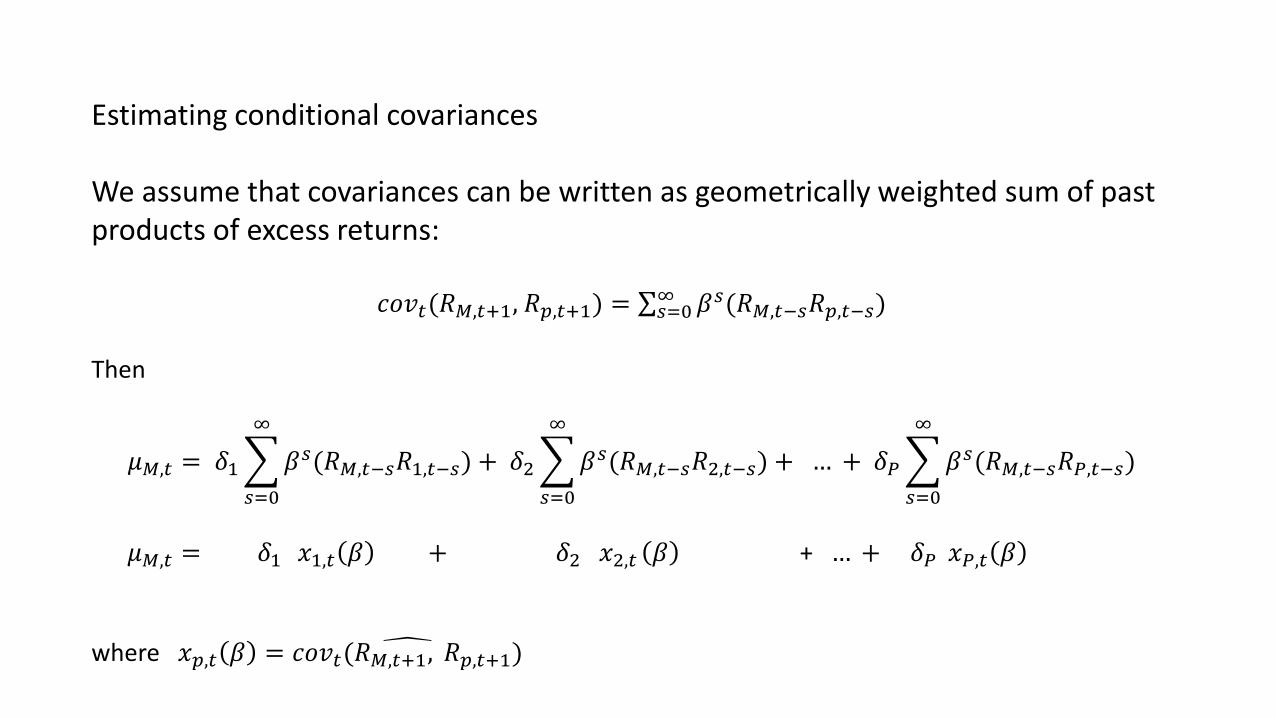
Estimating conditional covariances
We assume that covariances can be written as geometrically weighted sum of past products of excess returns:
𝑐𝑜𝑣𝑡(𝑅𝑀,𝑡+1, 𝑅𝑝,𝑡+1) = σ𝑠=0∞ 𝛽𝑠(𝑅𝑀,𝑡−𝑠𝑅𝑝,𝑡−𝑠)
Then
𝜇𝑀,𝑡 = 𝛿1
𝑠=0
∞
𝛽𝑠(𝑅𝑀,𝑡−𝑠𝑅1,𝑡−𝑠) + 𝛿2
𝑠=0
∞
𝛽𝑠(𝑅𝑀,𝑡−𝑠𝑅2,𝑡−𝑠) + … + 𝛿𝑃
𝑠=0
∞
𝛽𝑠(𝑅𝑀,𝑡−𝑠𝑅𝑃,𝑡−𝑠)
𝜇𝑀,𝑡 = 𝛿1 𝑥1,𝑡 𝛽 + 𝛿2 𝑥2,𝑡 𝛽 + … + 𝛿𝑃 𝑥𝑃,𝑡 𝛽
where 𝑥𝑝,𝑡 𝛽 = 𝑐𝑜𝑣𝑡(𝑅𝑀,𝑡+1, 𝑅𝑝,𝑡+1)

Estimation equation:
𝑅𝑀,𝑡+1 − 𝑅𝐹,𝑡 = 𝑎0 + 𝑎1𝑥1,𝑡 𝛽 + 𝑎2𝑥2,𝑡 𝛽 + … + 𝑎𝑃𝑥𝑃,𝑡 𝛽
Estimation procedure:
1. Choose pricing kernel e.g. CAPM, FF3
2. Choose value for β
3. Calculate covariance estimates 𝑥𝑝𝑡 𝛽 = σ𝑠=0∞ 𝛽𝑠(𝑅𝑀,𝑡−𝑠𝑅𝑝,𝑡−𝑠)
4. Run OLS regression of market excess return on covariance estimates 𝑥𝑝𝑡 𝛽
5. Calculate R2
6. Iterate over β to find maximum R2
7. Compute significance levels, s.e’s, bias adjustment using bootstrap
Estimated covariances with market return

The return interval
• Increasing prediction horizon tends to increase predictive R2
• But more precise estimates of covariances possible with short return intervals
• However theory implies relevant return interval for covariances of returns should be same as prediction horizon• NB covariances of arithmetic returns do not scale with return interval• Returns not iid and lagged cross-correlations of returns
• As compromise, compute covariances using lagged 1–quarter returns to predict 1-quarter return
• Persistence in μ means this covariance will also predict 1 year returns (estimates of 1-year covariances unreliable)
• Compare with results using 1-month lagged returns to calculate covariances

Data
FF aggregate market factor
𝑅𝐹𝑡 - 1-month T-bill rate compounded
𝑅𝑀𝑡 difference between market factor and 𝑅𝐹𝑡
Pricing kernel portfolios• Market
• FF3F
• Zero – market + zero dividend portfolio
• Growth – market + average return on (sl, bl)
• Sample 1946 – 2016• Predictions: 1954.1 – 2016.4

Predicting 1- quarter market excess returns
KernelPortfolios
a0 RM SMB HML β R2 R2c p-value
M 0.00(0.01)
1.34(0.44)
0.45(0.26)
0.04 0.04 0.01
FF3F -0.00(0.01)
1.65(0.51)
-1.18(0.97)
1.50(0.82)
0.61(0.23)
0.07 0.06 0.00
Predicting 1- year market excess returns
M 0.04(0.09)
3.00(1.36)
0.35(0.30)
0.04 0.03 0.21
FF3F 0.03(0.12)
6.11(2.15)
-10.02(3.82)
5.52(3.02)
0.52(0.22)
0.19 0.17 0.00
s.e. in parens.

17% R2 for 1 year predictions compares with the following R2 for prior predictors
Divyld Earnings yield
Book/Mkt
Value Spread
Glamor Stock Variance
T-Billrate
Long term yld
0.04 0.01 0.01 0.03 0.05 0.01 0.01 0.00
TermSpread
Inflation DefaultSpread
Kelly-Pruitt
Guo &Savickas
cay hjtzSentiment
Shortinterest
0.04 0.02 0.02 0.05 0.03 0.07 0.08 0.08

Constant 0.00(0.00)
0.17(1.59)
0.28(1.31)
Div yield 0.04(1.82)
0.03(1.47)
Glamor -0.03(1.9)
-0.03(1.90)
Kelly-Pruitt 0.00(0.02)
0.01(0.24)
cay 0.06(2.76)
0.04(2.37)
FF3F prediction 1.00(5.94)
0.82(4.52)
R2 0.19 0.17 0.29
Throwing all the major predictors into the predictive regression:
Only cay is significant but much less strong than FF3F (t-stats in parentheses)

Inspection of the FF portfolios reveals we can get strong results with just two portfolios in the pricing kernel: the market portfolio and either
• Growth = (sl + bl)/2
Or
• Zero = the zero dividend yield portfolio
Predicting 1- year market excess returns
KernelPortfolios
a0 RM Growth Zero β R2 R2c p-value
Growth 0.03(0.01)
25.2(5.99)
-18.6(4.79)
0.51(0.29)
0.16 0.15 0.01
Zero 0.03(0.07)
16.8(4.25)
-9.90(2.73)
0.58(0.26)
0.19 0.18 0.00
s.e. in parens.
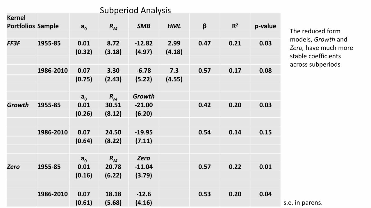
Kernel Portfolios Sample a0 RM SMB HML β R2 p-value
FF3F 1955-85 0.01 8.72 -12.82 2.99 0.47 0.21 0.03(0.32) (3.18) (4.97) (4.18)
1986-2010 0.07 3.30 -6.78 7.3 0.57 0.17 0.08(0.75) (2.43) (5.22) (4.55)
a0 RM GrowthGrowth 1955-85 0.01 30.51 -21.00 0.42 0.20 0.03
(0.26) (8.12) (6.20)
1986-2010 0.07 24.50 -19.95 0.54 0.14 0.15(0.64) (8.22) (7.11)
a0 RM ZeroZero 1955-85 0.01 20.78 -11.04 0.57 0.22 0.01
(0.16) (6.22) (3.79)
1986-2010 0.07 18.18 -12.6 0.53 0.20 0.04(0.61) (5.68) (4.16)
The reduced form models, Growth and Zero, have much more stable coefficients across subperiods
Subperiod Analysis
s.e. in parens.

-20
-10
0
10
20
30
40
50
19
54
19
55
19
57
19
58
19
60
19
61
19
63
19
64
19
66
19
67
19
69
19
70
19
72
19
73
19
75
19
76
19
78
19
79
19
81
19
82
19
84
19
85
19
87
19
88
19
90
19
91
19
93
19
94
19
96
19
97
19
99
20
00
20
02
20
03
20
05
20
06
20
08
20
09
20
11
20
12
20
14
20
15
1 year expected returns from pricing kernel model
PKM(FF3) PKM(G) PKM(Zero)
Correlations: FF3F, Growth 0.96; FF3F, Zero 0.87

Expected Return Series
• Mean 1 year expected return 7.4%
• Peaks
• 1955.2 27% (21%) Formosa crisis
• 1962.4 26% (20%) Cuban missile crisis
• 1974.3 32% (40%) First oil crisis
• 1987.4 22% (32%) Lehman Bros.
• Negative
• Around the millennium (dot.com)• 1973-4 (Cf. Boudoukh et al. 1993)
From FF3F (Zero) model

Pseudo R2 for 1-year out of sample forecasts - 1965-2016
FF3F Growth Zero
9.4% 13.8% 16.1%
• And the reduced form models perform better in out of sample forecasts
• Previous results• Kelly-Pruitt (2013): 3.5-13.1% for 1980-2010• Rapach et al. (2016) short interest predictor: 13.2% for 1990-2014.

Discount Rate Model
• Provides further check on Pricing Kernel Model
• Allows us to distinguish cash flow news from discount rate news
• We shall show that it is changing covariance with cash flow news that is driving changing expected returns

Discount Rate Model – intuition
For a bond, if we know:its initial yield, and the time series of returns (changes in yield)
Then we know its current yield and expected return
100 100
Tt
The problem is more difficult for stocks –because returns affected by news about cash flows as well as about discount rates.
We shall use returns on several portfolios to soak up cash flow news and isolate discount rate news
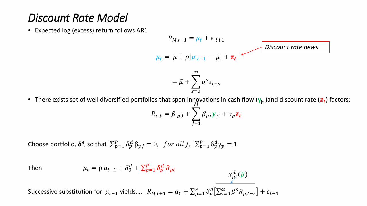
Discount Rate Model• Expected log (excess) return follows AR1
𝑅𝑀,𝑡+1 = 𝜇𝑡 + 𝜖 𝑡+1
𝜇𝑡 = ҧ𝜇 + 𝜌 𝜇 𝑡−1 − ҧ𝜇 + 𝒛𝒕
= ҧ𝜇 +
𝑠=0
∞
𝜌𝑠𝑧𝑡−𝑠
• There exists set of well diversified portfolios that span innovations in cash flow (yjt )and discount rate (𝒛𝒕) factors:
𝑅𝑝,𝑡 = 𝛽 𝑝0 +
𝑗=1
𝑀
𝛽𝑝𝑗𝒚𝑗𝑡 + 𝛾𝑝𝒛𝒕
Choose portfolio, δd, so that σ𝑝=1𝑃 𝛿𝑝
𝑑 β𝑝𝑗 = 0, 𝑓𝑜𝑟 𝑎𝑙𝑙 𝑗, σ𝑝=1𝑃 δ𝑝
𝑑γ𝑝 = 1.
Then 𝜇𝑡 = ρ 𝜇𝑡−1 + 𝛿0𝑑 + σ𝑝=1
𝑃 𝛿𝑝𝑑 𝑅𝑝𝑡
Successive substitution for 𝜇𝑡−1 yields…. 𝑅𝑀,𝑡+1 = 𝑎0 + σ𝑝=1𝑃 𝛿𝑝
𝑑 σ𝑠=0∞ 𝛽𝑠𝑅𝑝,𝑡−𝑠 + 휀𝑡+1
Discount rate news
𝑥𝑝𝑡𝑑 𝛽

Empirical discount rate model:
𝑅𝑀,𝑡+1 = 𝑎0 +𝑝=1
𝑃
𝛿𝑝𝑑𝑥𝑝𝑡
𝑑 𝛽 + 휀𝑡+1
where 𝑥𝑝𝑡𝑑 𝛽 = σ𝑠=0
∞ 𝛽𝑠𝑅𝑝,𝑡−𝑠.
Estimation as for pricing kernel model
RHS `spanning portfolios’:
Market and pricing kernel portfolios for FF3F, Growth and Zero

a0 RM m_FF3F m_Growth m_Zero β R2 p-value
0.08 -0.42 1.88 0.98 0.10 0.05
(0.03) (0.16) (1.89)
0.1 -0.51 2.66 0.99 0.14 0.01
(0.03) (0.16) (2.00)
0.07 -0.50 2.11 0.82 0.09 0.07
(0.03) (0.18) (2.04)
Discount Rate Model 1954-2016
s.e. in parens.

-15
-10
-5
0
5
10
15
20
25
30
19
54
19
55
19
57
19
58
19
60
19
61
19
63
19
64
19
66
19
67
19
69
19
70
19
72
19
73
19
75
19
76
19
78
19
79
19
81
19
82
19
84
19
85
19
87
19
88
19
90
19
91
19
93
19
94
19
96
19
97
19
99
20
00
20
02
20
03
20
05
20
06
20
08
20
09
20
11
20
12
20
14
20
15
1 year Expected Returns from Discount Rate Model
DRM(FF3) DRM(Growth) DRM(Zero)
-20
-10
0
10
20
30
40
50
19
54
19
55
19
57
19
58
19
60
19
61
19
63
19
64
19
66
19
67
19
69
19
70
19
72
19
73
19
75
19
76
19
78
19
79
19
81
19
82
19
84
19
85
19
87
19
88
19
90
19
91
19
93
19
94
19
96
19
97
19
99
20
00
20
02
20
03
20
05
20
06
20
08
20
09
20
11
20
12
20
14
20
15
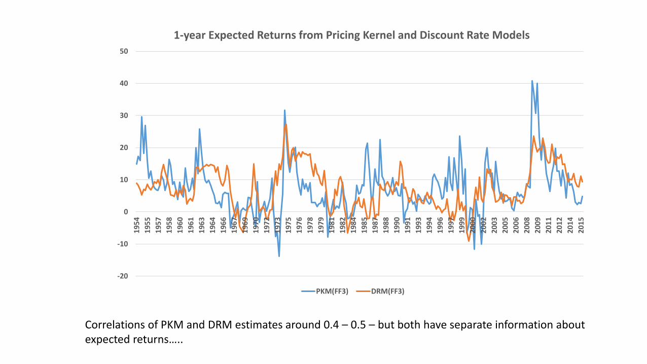
1-year Expected Returns from Pricing Kernel and Discount Rate Models
PKM(FF3) DRM(FF3)
Correlations of PKM and DRM estimates around 0.4 – 0.5 – but both have separate information about expected returns…..
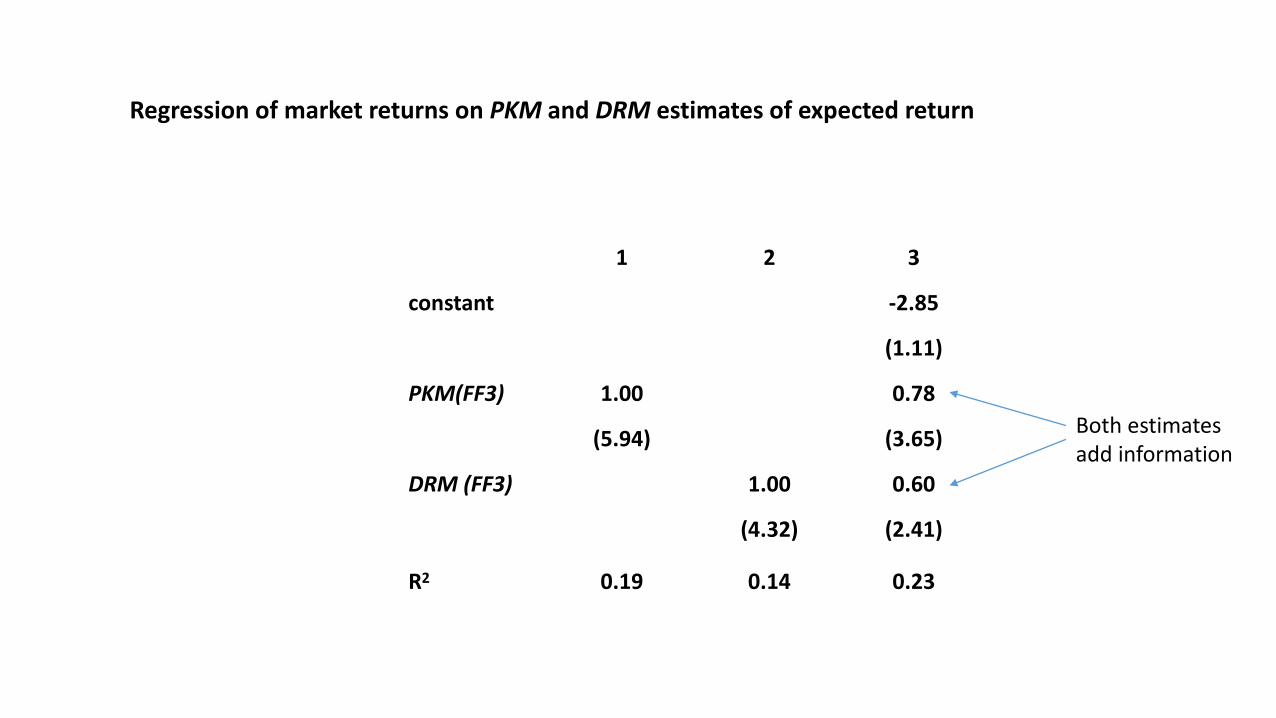
Regression of market returns on PKM and DRM estimates of expected return
1 2 3
constant -2.85
(1.11)
PKM(FF3) 1.00 0.78
(5.94) (3.65)
DRM (FF3) 1.00 0.60
(4.32) (2.41)
R2 0.19 0.14 0.23
Both estimatesadd information

The BIG issue
The market moves because of
• new information about future cash flows – cash flow news
• new information about future expected returns – discount rate news
Our discount rate model gives us a direct estimate of cash flow news - zt
This enables us to ask:
Is it time-varying risk of cash flow news or time varying risk of discount rate news that is driving time-varying expected returns?

A Cash Flow News Pricing Kernel Model
• Define cash flow news as the component of 𝑅𝑀 that is orthogonal to discount rate news, zt
• We have three estimates of zt corresponding to our 3 different discount rate models, FF3, Growth, Zero.
• So we have three different estimates of cash flow news obtained by regressing 𝑅𝑀on zt (FF3), zt (Growth), zt (Zero).
• Call them CFN(FF3), CFN(Growth) and CFN(Zero)
Then consider the following cash flow news version of the pricing kernel model:
𝑅𝑀,𝑡+1 − 𝑅𝐹,𝑡 = 𝑎0 + 𝑎1𝑥𝑡 𝛽
where 𝑥𝑡 𝛽 = σ𝑠=0∞ 𝛽𝑠(𝑅𝑀,𝑡−𝑠𝐶𝐹𝑁𝑡−𝑠)
We shall estimate it for the three different estimates of cash flow news

a0 CFN(FF3F) CFN(Growth) CFN(Zero) β R2 p-value
0.04 22.3 0.60 0.21 0.00
(0.05) (6.44)
0.04 19.1 0.60 0.18 0.00
(0.06) (13.23)
0.03 23.0 0.65 0.21 0.00
(0.05) (6.78)
Cash Flow News Pricing Kernel Model
s.e. in parens.
, 𝑥𝑡 𝛽 = σ𝑠=0∞ 𝛽𝑠(𝑅𝑀,𝑡−𝑠𝐶𝐹𝑁𝑡−𝑠)
RM SMB HML β R2 p-value
M 0.04(0.09)
3.00(1.36)
0.35(0.30)
0.03 0.21
FF3F 0.03(0.12)
6.11(2.15)
-10.02(3.82)
5.52(3.02)
0.52(0.22)
0.17 0.00
𝑅𝑀,𝑡+1 − 𝑅𝐹,𝑡 = 𝑎0 + 𝑎1𝑥𝑡 𝛽
For comparison
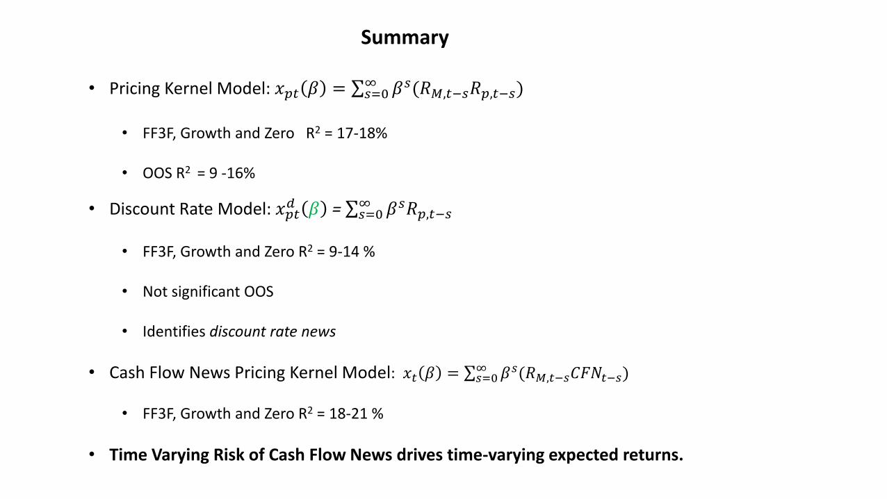
Summary
• Pricing Kernel Model: 𝑥𝑝𝑡 𝛽 = σ𝑠=0∞ 𝛽𝑠(𝑅𝑀,𝑡−𝑠𝑅𝑝,𝑡−𝑠)
• FF3F, Growth and Zero R2 = 17-18%
• OOS R2 = 9 -16%
• Discount Rate Model: 𝑥𝑝𝑡𝑑 𝛽 = σ𝑠=0
∞ 𝛽𝑠𝑅𝑝,𝑡−𝑠
• FF3F, Growth and Zero R2 = 9-14 %
• Not significant OOS
• Identifies discount rate news
• Cash Flow News Pricing Kernel Model: 𝑥𝑡 𝛽 = σ𝑠=0∞ 𝛽𝑠(𝑅𝑀,𝑡−𝑠𝐶𝐹𝑁𝑡−𝑠)
• FF3F, Growth and Zero R2 = 18-21 %
• Time Varying Risk of Cash Flow News drives time-varying expected returns.