Expected Inflation and the Constant-Growth Valuation Model

VOLUME 20 | NUMBER 2 | spRiNg 2008

APPLIED CORPORATE FINANCEJournal of

A M O R G A N S T A N L E Y P U B L I C A T I O N

In This Issue: Valuation and Corporate portfolio Management

Corporate portfolio Management RoundtablePresented by Ernst & Young

8 Panelists: Robert Bruner, University of Virginia; Robert Pozen,

MFS Investment Management; Anne Madden, Honeywell

International; Aileen Stockburger, Johnson & Johnson;

Forbes Alexander, Jabil Circuit; Steve Munger and Don Chew,

Morgan Stanley. Moderated by Jeff Greene, Ernst & Young

Liquidity, the Value of the Firm, and Corporate Finance 32 Yakov Amihud, New York University, and

Haim Mendelson, Stanford University

Real Asset Valuation: A Back-to-Basics Approach 46 David Laughton, University of Alberta; Raul Guerrero,

Asymmetric Strategy LLC; and Donald Lessard, MIT Sloan

School of Management

Expected Inflation and the Constant-Growth Valuation Model 66 Michael Bradley, Duke University, and

Gregg Jarrell, University of Rochester

Single vs. Multiple Discount Rates: How to Limit “Influence Costs” in the Capital Allocation process

79 John Martin, Baylor University, and Sheridan Titman,

University of Texas at Austin

The Era of Cross-Border M&A: How Current Market Dynamics are Changing the M&A Landscape

84 Marc Zenner, Matt Matthews, Jeff Marks, and

Nishant Mago, J.P. Morgan Chase & Co.

Transfer pricing for Corporate Treasury in the Multinational Enterprise 97 Stephen L. Curtis, Ernst & Young

The Equity Market Risk premium and Valuation of Overseas investments 113 Luc Soenen,Universidad Catolica del Peru, and

Robert Johnson, University of San Diego

stock Option Expensing: The Role of Corporate governance 122 Sanjay Deshmukh, Keith M. Howe, and

Carl Luft, DePaul University

Real Options Valuation: A Case study of an E-commerce Company 129 Rocío Sáenz-Diez, Universidad Pontificia Comillas

de Madrid, Ricardo Gimeno, Banco de España, and

Carlos de Abajo, Morgan Stanley

he Constant-Growth model is a discounted cash flow method of valuing companies and their projects that is taught in all top-tier business schools and used widely throughout the finan-

cial community. It is found in virtually all graduate-level corporate finance textbooks and valuation manuals. But, as we found during an extensive review of this literature, there has no been careful, systematic analysis of the effects of infla-tion on this model.1 As we show in the pages that follow, the failure to account properly for the effects of inflation has led to what academics call a “misspecification,” and thus an incorrect use, of the model in a particular set of cases—those where a company is assumed either to make no net new investments or to invest only in zero net present value (NPV) projects. We show that the error produced by this misapplication of the model is significant even at moderate levels of expected inflation.

In addition to its reliance on operating cash flows rather than earnings or P/E multiples, the main appeal of the Constant-Growth valuation model is its simplicity. As shown in Equation (1),

(1)10

FCFV

W G=

−

the market value of the firm (V0)

is a function of just three vari-

ables: the expected free cash flows in the next (or first future) period (FCF

1); the firm’s cost of capital (W); and the projected

growth rate of the firm’s future free cash flows (G).2 This model, which can be found in virtually all finance textbooks, is always written in nominal terms as in Equation (1).3

We have no quarrel with this equation. It is simply the formula for a growing perpetuity. Rather, our quarrel is with

by Michael Bradley, Duke University, and Gregg A. Jarrell, University of Rochester

Tthe incorrect transformations of this formula found throughout the valuation literature for the value of a company that makes no new investments or invests only in zero NPV projects.

Perhaps the most common application of the Constant-Growth model is its use in estimating what is referred to in the valuation literature as a company’s “continuation value” or, alternatively, its “terminal value.” When valuing a company, it is standard practice to estimate a company’s free cash flows over a finite (say, five-year) forecast period, and then assume that the firm will simply earn its cost of capital thereafter. The justification for this practice is the standard assumption of financial economists that the arrival of competitors, along with technological innovation and obsolescence, cause above-normal returns to become normal returns over time, and that, after the forecast period, the firm will earn a normal rate of return on its investments into perpetuity. The continuation value, as given by Equation (1), is the present value of the expected free cash flows beyond the forecast period into perpetuity.4

The assumption that the company will earn only normal rates of return during the post-forecast period is equiva-lent to assuming that either the firm will make no new net investments—that is, capital expenditures will equal depreci-ation—or that any investments that are made will have zero NPVs. Using this “zero-rent” argument, financial economists often assert that the terminal value of the firm can be estimated by a simple perpetuity of next period’s free cash flows, with the capitalization rate being the firm’s nominal cost of capital. This formulation is equivalent to setting G, the nominal growth rate in Equation (1), equal to zero:

(2)10

FCFV

W

* We thank Michael Barclay, John Coleman, Magnus Dahlquist, Doug Foster, Jennifer Francis, John Graham, Campbell Harvey, David Hsieh, Albert “Pete” Kyle, Richmond Mathews, Michael Moore, Stephen Penman, Michael Roberts, Frank Torchio, S. “Vish” Viswanathan and Ross Watts for helpful comments. We have benefited from many dis-cussions over the years regarding these and related issues with Robert Dammon, Tim Eynon, and, especially, Al Rappaport.

1. The popular valuation texts, Rappaport (1998), Copeland, Koller and Murin (1994) and Cornell (1993) all discuss various aspects of the effects of inflation on the valuation process. However, none develops the effects of inflation on the Constant-Growth model from first principles, as we do in this paper. This is also the case for the leading textbook in the field, Brealey, Myers and Allen (2006). Our analysis most closely resembles that of Rappaport. On page 47 he presents a formula for a “perpetuity with inflation” that is equivalent to an important relation that we develop in this paper.

2. According to Brealey, Myers and Allen, p. 65, this formula was first developed in 1938 by J.B. Williams and rediscovered in 1956 by M.J. Gordon and E. Shapiro. It is often called the Gordon Growth Model.

3. Throughout this paper we adopt the convention of stating nominal variables in up-per-case letters and real variables in lower-case letters. Also, since the models developed herein are forward-looking, all rates should be thought of as expectations.

4. Rappaport (1998) refers to the continuing value as the firm’s residual value, pp. 40-47. Also see Copeland et al. (1994), Chapter 9, “Estimating Continuing Value,” and Cornell (1993), Chapter 6, “Estimating the Continuing Value at the Terminal Date.” It should be noted that the continuing value as given by Equation (1) is the value of the firm at the end of the forecast period. Thus, in order to find the present value as of to-day, the terminal value has to be discounted by (1+W)T, where T is the end of the last forecast period.

66 Journal of Applied Corporate Finance • Volume 20 Number 2 A Morgan Stanley Publication • Spring 2008

Expected Inflation and the Constant-Growth Valuation Model*

We accordingly refer to this version of Equation (1) as the Zero-Nominal-Growth (“ZNG”) model.

Use of the ZNG model, or the simple perpetuity formula, is typically justified by the following reasoning: (1) with zero net new investments, there will be no growth; and (2) growth through the acceptance of zero NPV projects does not affect the (present) value of the firm. Therefore, under either condi-tion, it is appropriate to set G = 0 in Equation (1) and rely on Equation (2). Although this logic might appear to be sound, we show that this ZNG model is based on a mistaken specification of the nominal growth in free cash flows—G in Equation (1)—in the presence of inflation.

Specifically, the generally accepted expression for the value of a “zero-investment” or a “zero-NPV” firm—as presented throughout the finance literature and typically applied in practice—ignores the effect of inflation on the company’s total (accumulated) invested capital. In the traditional Constant-Growth model without inflation, if there is no new investment, there is no growth. However, in the presence of inflation, the value of the initial invested capital will grow at the rate of infla-tion. And, assuming a constant real return on invested capital and the replenishment of depreciated assets, the company’s (nominal) free cash flows stemming from those investments will grow at the same rate. In other words, the proper applica-tion of the Constant-Growth model is based on the market or replacement value of assets, which of course is affected by infla-tion. By ignoring the effects of expected inflation, the generally accepted expression—Equation (2)— understates the true value of the firm. And the higher the rate of inflation relative to the real cost of capital, the greater the understatement.

We develop the appropriate expression for the nominal growth in cash flows in the presence of inflation and show that the correct model assuming either zero investments or zero net present value investments is not the ZNG model, but rather the traditional Constant-Growth model, with the nominal growth rate set equal to the rate of inflation. We also show that this expression for the nominal growth term yields a valuation model that is independent of expected inflation.5

A second contribution of this paper to the valuation literature is an analysis of the effects of expected inflation on a company’s weighted-average cost of capital (WACC), the discount factor most often associated with the Constant-Growth model. We find that the WACC methodology (at least in its classic form, as developed by Miller and Modigli-ani) is incorrect if expected inflation is positive. Substituting nominal values into the M&M WACC equation results in an

overvaluation of the firm. We develop a correction factor that, when added to the (nominal) M&M WACC formula, yields a company’s true nominal WACC in the face of inflation.6 Finally, to complete our analysis, we show that the nominal WACC model developed by two finance academics—James Miles and John Ezzell—is compatible with any level of growth, whether attributable to inflation or real investments.7

The Constant-Growth Model with InflationOur analysis of the effects of inflation on the Constant-Growth model begins with a derivation of an expression for the firm’s nominal free cash flows (FCF

t). We then derive

an expression for the growth in nominal cash flows (G). We defer our discussion of the appropriate discount rate (W) until our later discussion of the firm’s WACC. For present purposes, suffice it to say that in the subsequent analysis, we assume that the firm’s nominal cost of capital (W) is consis-tent with the Fisher Equation:

W w w= + + (3)

where w is the firm’s real cost of capital and Π is the expected rate of inflation.8

The Real Return on Investment, net Cash Flows, and Free Cash Flows We begin our derivation of free cash flows with the following definition of the real return on investment (r):

(4)

tNCFr

(1=

+ t 1)K −

where NCFt is the firm’s net cash flow at the end of period t

and Kt-1

is its total capital stock at the beginning of the period. Rearranging Equation (4) yields:

t t 1NCF K r(1 ) (5)

Equation (5) states that the net cash flow to the firm in period t is given by the amount of capital at the beginning of the period (K

t-1), times the constant real return on investment

(r), times 1 plus the rate of inflation.9 Free cash flow in any period equals the firm’s net cash flow for the period less any net new investment:

t t tFCF NCF NNI (6)

5. If by “inflation” we mean a proportionate increase in all nominal interest rates and the prices of all goods and services, then expected inflation should have no effect on present values, i.e., present values should be inflation neutral.

6. One might be tempted to speculate that these two errors are offsetting, since the error in the ZNG model leads to an underestimate of the value of the firm and the er-ror in the M&M WACC leads to an overestimate. However, as developed subsequently, the adjustment to the ZNG model is to subtract Π, the rate of inflation, from W in the denominator of Equation (2), whereas the adjustment to the M&M model is to add tXΠL

to W in Equation 1, where tX is the firm’s tax rate and L is its debt to value ratio. Since both tX and L are less than 1.0, the M&M adjustment is much smaller than the adjust-ment to the ZNG model.

7. Miles and Ezzell (1980)8. Irving Fisher (1930). Also see Brealey, Myers and Allen, pages 116-118. 9. Recall that we have adopted the convention of expressing nominal variables in

upper-case letters and real variables in lower-case letters and that all rates and future values should be interpreted as expectations.

Journal of Applied Corporate Finance • Volume 20 Number 2 A Morgan Stanley Publication • Spring 2008 67

Define k as the firm’s plowback rate, which is the fraction of NCFt that is retained by the firm to finance net new investments:10

(7)

t

t

NNIk

NCF

Substituting Equation (7) into Equation (6) yields:

tFCF NCF t (1 k) (8)

The Growth in Free Cash FlowsClearly, a critical parameter in the Constant-Growth model is G, the projected constant growth in the firm’s free cash flows. In Appendix A we derive the expression for the growth in free cash flows based on two assumptions: (1) the (expected) real return on investment, as defined in Equation (4) above, remains constant; and (2) the Fisher Equation holds such that the nominal return on investment (R) can be written as:

R r r (9)

where r is the expected real return on investment and Π is the expected rate of inflation.

Making these assumptions, we develop the following expression for the growth in the firm’s free cash flows:

G = k R + ( 1 - k ) (10)

The first term in Equation (10) represents the growth in the firm’s free cash flows from new investments. The second term represents the increase in cash flows attributable to the increase in the nominal value of the firm’s fixed and working capital that results solely from inflation. Thus, there are two forces that account for the growth in nominal cash flows. The first is the increase in cash flows due to the nominal return on new investments. The second is the increase in nominal cash flows due to the fact that the nominal value of the firm’s capital stock is higher by the rate of inflation. As we demon-strate later, it is this second term that is ignored in the existing finance literature—in other words, according to the literature, G = k R.

As indicated by Equation (10), the effect of inflation on a company’s stock of capital will depend on the percentage of cash flows that are reinvested in the firm (k). If the plowback rate is zero (k = 0), then G = Π and all growth is attributable to the nominal growth in the company’s initial fixed and working capital stemming from inflation.11 Under these conditions, the firm’s total invested capital invested will remain constant in real terms into perpetuity. If the plowback rate k > 0, then

the inflationary growth of the company’s invested capital will be augmented by the nominal growth from new investments. Finally, if k = 1, the firm is plowing back its entire net cash flows. Consequently, the firm will generate no free cash flows into perpetuity and therefore would be theoretically worthless, since by assumption there would never be a distribution to security holders.12 However, when k = 1, the value of the firm will grow with the value of its capital stock, which, as given by Equation (10), will equal its nominal return on investment R. The value of the firm will continue to grow at this rate until the firm is liquidated.

In addition to Equation (10), the analysis in Appendix A develops three additional relations that will be helpful in our subsequent analysis. Consistent with the Fisher Equation we show that:

G g g

g k r

G kr

k r

(11)

and that: G g g

g k r

G kr

k r

(12)

where k is the firm’s plowback rate, r is the real return on investment and g is the real growth rate. Substituting Equa-tion (12) into Equation (11) yields:

G g g

g k r

G kr

k r (13)

Transformations of the Constant-Growth ModelWe now derive the appropriate expressions for the two most frequent transformations of the Constant-Growth model found in the finance literature: the value of a company that either (1) makes no net new investments or (2) accepts only zero NPV projects. As we demonstrate below, these two conditions yield the same valuation expression.

Zero InvestmentsThe value of the firm, according to the Constant-Growth model, assuming zero net new investment, is found by substi-tuting Equation (8) into the numerator of Equation (1), substituting G from Equation (10) into the denominator of this equation, and setting k, the reinvestment rate, equal to zero:

10

NCF (1 k)V

W (kR (1 k) ) )41(

10V

W

NCF )51(

(14)

(15)

10

NCF (1 k)V

W (kR (1 k) ) )41(

10V

W

NCF )51(

10. It follows that (1-k) is the firm’s payout ratio.11. See Appendix A for a demonstration of this proposition. 12. This is equivalent to the value of a zero coupon bond that never matures.


The intuition behind Equation (15) is that even though the firm makes no net new investments (k = 0), it still makes replacement investments sufficient to offset its economic depreciation, so that the real net cash flows must be constant over time.13 Thus, the future nominal cash flows (revenues, costs, and profits) emanating from a stream of constant real NCFs logically must be projected to grow at the rate of infla-tion, as is reflected in Equation (15).

We refer to this valuation equation as the Zero-Real-Growth (“ZRG”) model, since the formula is equivalent to assuming that k = 0 and therefore g = 0 in Equation (12), which implies that the real growth in cash flows is equal to zero. This in turn implies that all observed growth is attribut-able to inflation, which justifies our designation of this model as the ZRG model. (Of course, we could have just as easily labeled this expression the Inflationary-Growth model.)

The ZRG model is inflation neutral in that it generates a value for the firm that is independent of the level of expected inflation. To see this, note that the formula can be written exclusively in real terms. Given that W = w + Π + wΠ, it follows that W – Π = w (1+Π). Substituting this expression in the denominator and the expression for nominal cash flows into Equation (15) yields the following:

(16)1 10

ncf (1 ) ncfV

w(1 ) w= = )61(

Zero Net Present Value InvestmentsThe Constant-Growth model, under the assumption of zero net present value investments, is found by making the same substitutions as above and setting R = W:

110

NCF (1 k) NCF (1 k)V

0V

W (kR (1 k) ) W(1 k) (1 k)

1NCF

W (17)

Thus, the expression for the value of the firm when r = w (or equivalently R = W) is simply:

(18)

1 1 10

NCF ncf (1 ) ncfV

W w(1 ) w (18)

which, again, is the ZRG or Inflationary-Growth model. Note that real growth g is not necessarily zero under the zero NPV assumption. Indeed, since g = kr, if r = w > 0, then real growth g will be positive if k is positive. But any positive real growth that may be projected will not increase the value of the firm because all future investments have zero NPV (R = W and r = w). Hence, g is absent from Equation (17).

The preceding analysis demonstrates that the expression for the value of a zero-investment firm is the same as the expression for a zero-NPV firm—that is, Equations (15) and (17) are identical. This result—that the same expression is relevant for firms that either invest only in zero-NPV projects or invest nothing at all—will be useful later when we develop the appropriate discount factor for the Constant-Growth model under either of these conditions.

Review of the LiteratureIn this section we retrace the literature’s development of the expressions for the value of the firm assuming (1) zero net new investments and (2) investments only in zero NPV projects. The purpose is to demonstrate that the formulas found in the literature are incorrect when expected inflation is positive.

Zero InvestmentsThe expression for the value of a firm that makes no net new investments found in the literature is based on an erroneous expression for the growth in cash flows. Although incorrect, it is nevertheless common to define the nominal growth in net cash flows as:

G kR (19)

where R is the firm’s nominal return on investment.14 The correct expression for the growth in net cash flows, as we saw earlier in Equation (10), is:

G = k R + (1 - k) (20)

Again, it is the second term in this equation that is ignored in the literature. To derive what the literature describes as the zero-investment formula, simply substitute G from Equation (19) into Equation (1),

13. See Appendix A.14. Applying the Gordon Growth Model for the valuation of common stock, Brealey,

Myers and Allen write on page 65: 10

DIVP =

r - g

where P0 is the price of the stock at time 0, DIV1 is the (expected) dividend in period 1, r is the firm’s capitalization rate and g is the growth in dividends. It is important to note that BMA do not indicate whether r or g is stated in real or nominal terms. However, since DIV1 is presumably a nominal number, stated in period 1 dollars, we must presume that both r and g are nominal values. Instead of deriving an expression for g, the nominal growth in earnings, they simply assert on page 67:

“If Cascade earns 12 percent of book equity and reinvests 44 percent of income, then book equity will increase by .44 x .12 = .053, or 5.3 percent. Earnings and dividends

per share will also increase by 5.3%:Dividend growth rate = g = plowback ratio x ROE.” (Emphasis added.) Again, on page 69 they write: “Dividend growth rate = plowback

ratio x ROE.” Other references that assert that G=kR include: Ross, Westerfield and Jaffee, p.

128, Grinblatt and Titman, p. 832, Rao, p. 403, Bodie and Merton, p. 123, Emery and Finnerty, p. 149, Shapiro and Balbirer, p. 159, Benninga and Sarig, p. 9, Van Horn, pp. 30-31, Martin, Petty, Keown and Scott, p.123. It is interesting to note that none of these authorities feels compelled to prove this relation. They all rely on it as though it is self-evident. Not only is this expression for the nominal growth rate not self-evident, it is incorrect as we demonstrate by the derivation of Equation 10 in the text.


10

NCF (1 k)V

W kR )12(

(21)

and set k, the reinvestment rate, equal to zero.

10

NCFV

W )22( (22)

Equation (22) is what the finance literature defines as the “no-growth” value of the firm. For example, the most recent edition of a bestselling finance text describes Equation (22) as the value of a company “that does not grow at all. It does not plow back any earnings and simply produces a constant stream of dividends.”15 Another popular text states that the above expression “is the value of the firm if it rested on its laurels, that is, if it simply distributed all earnings to the stockholders.”16

While it may seem perfectly logical that with no net new investments a firm would generate a constant stream of cash flows into perpetuity, this reasoning ignores the effects of inflation on the firm’s initial invested capital. If a company’s investments simply keep up with obsolescence and economic depreciation, its total invested capital stock will increase at the rate of inflation; and, if we assume a constant real return on investment, its cash flows will also increase at the rate of inflation. Put simply, one cannot express the value of the firm as a perpetuity in nominal terms—which is what Equation (22) does—when inflation is positive. As we demonstrated earlier in Equation (15), the presence of inflation requires that the value of a zero-investment firm be expressed as a growing perpetuity, with the growth rate set equal to the rate of inflation.

To be clear, we are not implying that either the authors of the texts cited above or the rest of the finance profession are unaware of the effects of expected inflation on the value of capital assets. Indeed, in the most influential text in the profession, after the authors develop the Constant-Growth model, they present the Fisher Equation and admonish the reader to “Discount nominal cash flows at a nominal discount rate. Discount real cash flows at a real rate. Never mix real cash flows with nominal discount rates or nominal flows with real rates.”17 But the authors never revisit the Constant-Growth model and discuss how inflation impacts

the parameters of this model. Failure to do so has led to confusion in the valuation literature, particularly regard-ing the value of G and the values of companies that make no new investments or invest only in zero net present value projects.

We earlier labeled Equation (22) the Zero-Nominal-Growth model, since it is equal to Equation (1) with G, the nominal growth rate, set equal to zero. We also use the term to emphasize the internal inconsistency inherent in this expression. A Zero-Nominal-Growth model in a world of inflation is an economic oxymoron. Since inflation is the only distinction between real and nominal values, what does it mean to have inflation and zero nominal growth? Under reasonable assumptions, you can’t have both at the same time. Based on Equation (11) only under the highly unlikely and therefore mostly irrelevant case of a negative real growth rate—one that just offsets a positive rate of inflation—can you have zero nominal growth and positive inflation.18

Since expected inflation is almost always positive, the implication of negative real growth into perpetuity makes the Zero-Nominal-Growth model useless for most real-world valuation applications. In addition, the theoretical conditions under which real growth can be negative into perpetuity are unlikely to occur in practice. As Equation (13) indicates, a negative real growth rate implies that either the real return on investment (r) or the plowback ratio (k) is negative into perpetuity. Since the Constant-Growth model is forward looking, companies cannot be expected to accept a project with an ex ante negative return. Thus, a negative real growth rate must be due to a negative k, which repre-sents a steady liquidation of the firm over time. Obviously, this condition is not appropriate for most corporate valua-tion applications.19

Zero Net Present Value InvestmentsThe derivation of the expression for the value of a company that invests only in zero NPV projects found throughout the finance literature relies on the same mistaken expres-sion for the growth in nominal cash flows given in Equation (19). Zero NPV implies that R = W. Substituting Equations (8) and (19) into Equation (1) and imposing this zero-NPV condition (R = W) also yields the Zero-Nominal-Growth formula:

15. Brealey, Myers and Allen (2006), p. 73.16. Ross, Westerfield and Jaffee (1993), pp. 130-131. We have examined a number

of other texts and have been unable to find the expressions developed in this paper – expressions that are necessary for an inflation-neutral valuation model.

17. Brealey, Myers and Allen, p.118.18. Specifically, if g

1, then G = 0 even though Π > 0.

19. Of course k can be negative or, with an influx of capital, even be greater than 1 over a finite period. However, only in very rare circumstances can these extreme values of k persist into perpetuity.


(23)

1 1 10

NCF (1 k) NCF (1 k) NCF (1 kV

0V

W kR W kW W(1 k)

1NCF

W A number of financial economists have argued that

Equation (23) is the expression for the value of a firm that only invests in zero NPV projects.20 Although it may seem logical that since investments in zero NPV projects do not create value, G should not appear in Equation (23). Intuitively, the discounted value of cash flows from additional investments just equals the present value of the new investments assuming the return on investment equals the cost of capital. Thus, value is not created by these additional investments. And of course this logic is correct.

But, with positive inflation, the value of invested capital will grow at the rate of inflation and, assuming a constant real rate of return, the net cash flows from these investments (the numerator in Equation (23)) will also grow at the rate of infla-tion. The denominator in Equation (23) ignores this growth and therefore understates the value of the firm.

In sum, the correct expression for the value of the firm that invests in only zero NPV projects also must be a growing perpetuity with the growth rate equal to the rate of

inflation—what we have labeled the Zero-Real-Growth or Inflationary-Growth model.

The General ModelThus far, we have focused our analysis on two specific cases: (1) the value of a firm that makes no new investments; and (2) the value of a firm that invests only in zero NPV projects. But our criticisms of the treatment of inflation in the Constant-Growth model also apply to the estimation of G in general. As developed above, the expression for the growth in nominal cash flows that is found throughout the literature is:

G kR

G kR (1 k)

(24)

whereas the correct expression for the nominal growth term is

G kR

G kR (1 k)

(25)

To the extent that researchers and practitioners use the former expression to calculate G, they are understating the true value of the firm. Thus, our criticism of the Constant-Growth model, as it is presented in the literature, goes beyond the two special cases of zero NPV and zero investments. Our criticisms

Table 1 percentage Underestimate According to the Zero-nominal-Growth Model

Expected Rate of Inflation

0% 1% 2% 3% 4% 5% 6% 7% 8% 9% 10% 11% 12% 13% 14% 15%

1% 0 50 66 74 79 83 85 87 88 89 90 91 91 92 92 93

2% 0 33 50 59 66 70 74 77 79 81 82 83 84 85 86 87

3% 0 25 40 49 56 61 65 69 71 73 75 77 78 79 80 81

4% 0 20 33 42 49 54 59 62 65 67 69 71 73 74 75 77

5% 0 17 28 37 43 49 53 57 60 62 65 66 68 70 71 72

6% 0 14 25 33 39 44 49 52 55 58 60 62 64 66 67 68

7% 0 12 22 29 35 40 45 48 51 54 56 59 60 62 64 65

8% 0 11 20 27 32 37 41 45 48 51 53 55 57 59 61 62

9% 0 10 18 24 30 35 39 42 45 48 50 52 54 56 58 59

10% 0 9 16 23 28 32 36 40 43 45 48 50 52 53 55 57

11% 0 8 15 21 26 30 34 37 40 43 45 47 49 51 53 54

12% 0 8 14 20 24 28 32 35 38 41 43 45 47 49 51 52

13% 0 7 13 18 23 27 30 33 36 39 41 43 45 47 49 50

14% 0 7 12 17 22 25 29 32 35 37 39 41 43 45 47 48

15% 0 6 12 16 20 24 27 30 33 36 38 40 42 43 45 47

Rea

l Cos

t of

Cap

ital

20. Copeland, Koller and Murrin (1994), pp. 282-283. Rappaport (1998) p.42 also asserts that Equation (23) is the value of the firm if all of its projects have zero NPV. Cope-land et. al. pp. 513-515, derive the relation (stated in our notation) FCFt = NPVt ( 1 - k ). They then substitute G/R and write FCFt = NPVt ( 1 - G/R ). From this equation they follow the derivation as outlined in the text. Thus, these authors erroneously assume, like Brealey, Myers and Allen (2006), that k = G/R, when in fact the correct relation is k = g/r. This substitution leads them to Equation (23). It is important to note that Copeland et. al.

do not specify whether their variables are nominal or real. The clear implication though, is that they are all nominal values. Cornell (1993, p. 156) makes the same error. He explicitly states that G is the nominal rate of growth in free cash flows and distinguishes it from g, which he earlier defines on page 148 as the “long-run growth in real returns.” Nevertheless, Cornell assumes that k=G/R. Weston et. al. (1998, p. 186) make the same, erroneous substitution. Rappaport (1998, pp. 40-44) rationalizes Equation (23) verbally, making the same arguments that are embodied in the algebra above.


also apply to the general model, provided the growth term is calculated according to Equation (24) instead of Equation (25).

The Error Rate of the Zero-Nominal-Growth Model under Inflation As noted above, the Zero-Real-Growth (ZRG) model is infla-tion-neutral, since the model can be written exclusively in real terms, as we saw in Equation (18). But, somewhat ironically, the Zero-Nominal-Growth (ZNG) model, as presented in the literature, is not inflation-neutral. According to the model, the value of the firm is inversely related to expected inflation—that is, the higher expected inflation, the higher the discount factor and hence the lower the value of the firm.

The percentage by which the Zero-Nominal-Growth (ZNG) model understates the value of a firm with zero net new invest-ments or zero NPV investments can be readily calculated by sub tracting the ratio of Equation (22) to Equation (15) from 1:

ZNG

ZRG

V W–Percentage Underestimate = 1 = 1

WVw(1 )

Percentage Underestimate = 1 w(1 )

(26)

The entries in Table 1 illustrate the percentage under-valuation generated by the Zero-Nominal-Growth model for various levels of the real cost of capital (w) and the expected rate of inflation (Π). For example, if expected inflation is 2% and the real rate of return is 3%, then the Zero-Nominal-Growth model will underestimate the true value of the firm by 40%! In other words if the true value of the firm was $100, the Zero-Nominal-Growth formula will value the firm at $60. Note also that the undervaluation is greater when the expected rate of inflation is higher than the expected real interest rate. In other words, the values in the north-east triangle of the table are greater than those in the south-west triangle.

Expected Inflation and the Zero-Real-Growth Discount FactorWe now develop the appropriate discount factor for the Zero-Real-Growth model, W in Equations (15) and (17). Most of the valuation literature advocates the use of the weighted-average cost of capital (WACC) methodology developed by Miller and Modigliani (M&M), which is designed to account for the increase in the firm’s net cash flows stemming from the tax deductibility of interest payments.21 As we show, however, the M&M WACC model (equation) is not infla-

tion neutral when stated in nominal terms. We show that the equation systematically understates the true WACC and therefore overstates the value of the firm if expected inflation is positive. We provide an expression for this underestimate of the firm’s cost of capital that, when added to the M&M WACC formula, generates the correct discount factor for the Zero-Real-Growth (Inflationary-Growth) model. We show that using this correction factor generates a value of the firm that is independent of expected inflation.

There are two basic approaches to valuing the interest tax shields of a levered firm into perpetuity: the Adjusted Present Value (APV) method and the WACC method. The APV method recognizes that the value of a levered firm (V

L)

is equal to the value of the firm if it were un-levered (VU) plus

the present value of the interest tax shields (PVITS):

L UV = V + PVITS (27)

In general, the interest tax shield per period can be written as:

t X DITS = t W D (28)

where tX

is the corporate tax rate, WD

is the nominal cost of debt and D is the amount of debt outstanding at the begin-ning of the period.22

The main insight behind the alternative WACC method-ology is that under certain circumstances, the value of a levered firm can be found directly by discounting its future free cash flows by its tax-adjusted, weighted-average cost of capital. In other words, the value of a levered firm can be found by substi-tuting the following definition of WACC for W in Equations (15) and (17):

(29)V V

LX D E

LL

D EWACC ( 1 t ) W W

where E is the market value of equity, VL is the market value

of the levered firm (VL=D+E) and W L

E is the firm’s nominal

cost of (or required rate of return on) its levered equity.23 Because of the tax subsidy to debt financing, the value of

the firm increases with greater leverage. Intuitively, as the firm substitutes debt for equity, a greater weight is placed on the first term of Equation (29). Since t

X > 0 and W

D < WL

E, the

greater the debt-to-value ratio, the lower the WACC—and the lower the WACC, the higher the value of the firm.24 As already noted, under certain circumstances, the increase in the

21. “The appropriate rate for discounting the company’s cash flow stream is the weighted average of the costs of debt and equity capital,” Rappaport, page 37. Also see Brealey, Myers and Allen (2006), Chapter 19, Copeland et al., Chapter 8 and Cornell, Chapter 7.

22. If the bond is issued at par, the cost of debt would be the bond’s coupon rate.23. The analysis assumes that the firm can take full advantage of the tax deduction

of interest payments.

24. Of course, according to M&M, if markets are perfect and taxes are zero, then WLE

will adjust to offset exactly any change in weights, leaving WACC unchanged.


value of the firm caused by discounting its net cash flows by this lower rate—namely its WACC—is exactly equivalent to the present value of the debt tax shields created by the increase in debt financing, provided the cost of debt is unaffected by the increase in leverage.25

The Present Value of the M&M Tax Shields26

Under the assumptions of the M&M model, the firm’s cash f lows and the amount of debt outstanding are constant into perpetuity. The interest tax shield in Equation (28) is therefore a simple perpetuity. If we assume that the interest payments are as risky as the debt itself, the present value of this perpetuity is:

X D D XPVITS = ( t W D ) / W = t D.

L U XV = V + t D.

(30)

Thus, substituting Equation (30) into (27), under M&M,

(31)

X D D XPVITS = ( t W D ) / W = t D.

L U XV = V + t D.

The M&M WACC ModelThe M&M WACC model posits a relation between a firm’s cost of equity capital and its leverage. Specifically, the cost of equity to a levered firm is equal to the cost of capital if the firm was un-levered plus the difference between the un-levered cost of capital and the (constant) cost of debt times 1 minus the firm’s tax rate times the firm’s debt-to-equity ratio. Although this formula can be found in most corporate finance textbooks, like the Constant-Growth model in general, the authors never state whether this rela-tion holds for nominal or real variables.27 Unfortunately, this silence and the context in which the M&M model is typically presented in the literature clearly imply that the relation holds in nominal terms. But, as we show below, this is not correct.

The fact that the M&M model assumes fixed cash flows and a fixed amount of debt outstanding immediately raises doubts that the model holds in nominal terms. As we will see, this intuition is correct. Since the M&M model is based on the assumption of constant cash flows, it follows that the M&M WACC provides the correct valuation when stated in real terms. But, when stated in nominal terms, the M&M model systematically understates the firm’s true nominal WACC when expected inflation is positive. We provide an adjustment factor that, when added to the nominal M&M formula, makes it compatible with our Zero-Real-Growth (Inflationary-Growth) model.

Real WACC Under the Zero-Real-Growth AssumptionStating the M&M model in real terms, the cost of levered equity is equal to:

Lw wE U U D x

D(w w )(1 t )

E (32) (32)

where wU is the firm’s un-levered cost of capital.28 Substitut-ing Equation (32) into Equation (29) and solving for the real weighted average cost of capital yields:

M&MU Xwacc w (1 t L) (33)

where L is the firm’s debt-to-value ratio, L

D

V. Now, according

to the M&M model:

1UL XM&M

V V t Dwacc

fcf (34)

To see that Equation (34) holds, substitute Equation (33) for waccM&M and show that the resulting expression is equal to V

L:

1L

U X

fcfV =

w ( 1 t L ) (35)

Noting that 1U

U

fcfV

w

UL

X

V = ( 1 t L )

V (36)

(37)

Combining the above results, the value of a levered firm, assuming zero real growth, can be written as either Equation (34) or Equation (35), which implies the following:

(38)1L U X M&M

fcf V + t D = .

waccV =

In other words, the M&M model holds in real terms.

25. Note that the WACC methodology ignores bankruptcy costs and any other lever-age-related costs. In fact the M&M model assumes that WD is equal to the risk-free rate regardless of the degree of leverage. This is an obvious limitation to the M&M WACC model since there is ample empirical evidence that leverage and the cost of debt are positively related.

26. This analysis follows the presentation of the M&M WACC model in Brealey, Mey-ers and Allen (2006) pp. 517-520.

27. See references in Footnote 3.28. Note that we continue the convention of stating real variables in lower-case letters

and nominal values in upper-case letters.


Nominal WACC under the Zero-Real-Growth AssumptionThe assumptions of the basic M&M model imply that it is inflation neutral in that a change in expected inflation will not have any effect on the value of the firm. However the M&M equation, stated in nominal terms, is not inflation neutral.

Inflation neutrality requires that rates of return adhere to the Fisher Equation. Thus, for the nominal version of the M&M WACC to be inflation neutral, it must be the case that:

(39)TrueWACC = wacc + + wacc (39)

Substituting the definition of wacc from Equation (33) into (39) yields:

(40)TrueWACC (40) U x U Xw (1 t L) w (1 t L)

Stating the M&M WACC formula (Equation (33)) in nomi-nal terms:

M&MU XWACC W (1 t L) (41)

Invoking the Fisher Equation and substituting for WU,

M&MU U XWACC (w w ) (1 t L)

(42)

Expanding Equation (42)

(43)w (1 t L) w (1 t L) (1 t L)

M&MWACC

U X U X X

Re-writing Equation (40)

(44)

So that,

(45)

True M&MXWACC = WACC t L (46)

Equation (46) shows that the “true” nominal WACC is equal to the M&M WACC plus the term ∏t

X L. In other

words the M&M WACC under-states the appropriate value by the factor ∏t

X L. Intuitively, the nominal WACC model

assumes that an increase in inflation will increase the firm’s tax shield from debt financing. However, this violates a basic assumption of the M&M model that the amount of debt is fixed and independent of its cost of capital as illustrated in Equation (31).

Equation (46) also shows that it is easy to correct the nominal WACC formula so that it is consistent with the Fisher Equation and yields the correct value. One can simply add the amount ∏t

X L to the computed WACC using the standard

M&M nominal WACC formula. Adding the quantity ∏t

X L to the standard M&M WACC yields the correct nominal

WACC, which is consistent with the Fisher Equation.29

In Table 2 above we illustrate that the error generated by the nominal version of the M&M WACC equation is positively related to the expected rate of inflation and that the error is greater, the greater the firm’s leverage ratio. Intuitively, the nominal M&M model assumes correctly that an increase in

Table 2 Percentage Overvaluation from Using M&M Nominal Parameters

Expected Rate of Inflation

0% 1% 2% 3% 4% 5% 6% 7% 8% 9% 10% 11% 12% 13% 14% 15%

0% 0.0 0.0 0.0 0.0 0.0 0.0 0.0 0.0 0.0 0.0 0.0 0.0 0.0 0.0 0.0 0.0

10% 0.0 0.4 0.8 1.2 1.6 2.0 2.4 2.8 3.2 3.6 3.9 4.3 4.7 5.0 5.4 5.7

20% 0.0 0.9 1.7 2.6 3.5 4.3 5.2 6.0 6.9 7.7 8.6 9.4 10.3 11.1 12.0 12.8

30% 0.0 1.4 2.7 4.1 5.5 6.9 8.4 9.8 11.2 12.7 14.2 15.6 17.1 18.6 20.1 21.6

40% 0.0 1.9 3.9 5.9 7.9 10.0 12.1 14.2 16.4 18.7 20.9 23.3 25.6 28.1 30.5 33.1

50% 0.0 2.5 5.2 7.9 10.6 13.5 16.5 19.6 22.7 26.0 29.4 32.9 36.6 40.4 44.3 48.4

60% 0.0 3.2 6.6 10.1 13.8 17.7 21.8 26.0 30.5 35.3 40.3 45.5 51.1 57.1 63.3 70.0

70% 0.0 4.0 8.3 12.8 17.6 22.7 28.2 34.1 40.5 47.3 54.7 62.7 71.4 81.0 91.4 102.9

80% 0.0 4.9 10.2 15.9 22.1 28.9 36.3 44.5 53.5 63.5 74.8 87.4 101.7 118.0 136.9 158.9

Deb

t to

Val

ue

29. Although not shown, it should be noted that the nominal version of the M&M model is also vitiated if the real growth term is positive. Intuitively, the M&M model is incompatible with growth of any sort, be it from inflation or new investment.


inflation will increase the firm’s WACC. However, the model incorrectly assumes that the government will absorb the amount ∏t

X L of the increase. In fact, as discussed above, an increase in

the expected rate of inflation—at the time of valuation—will cause a proportionate increase in both the firm’s coupon rate and the cost of debt, leaving the (present) value of the debt tax shields, and hence the value of the firm, unaffected.

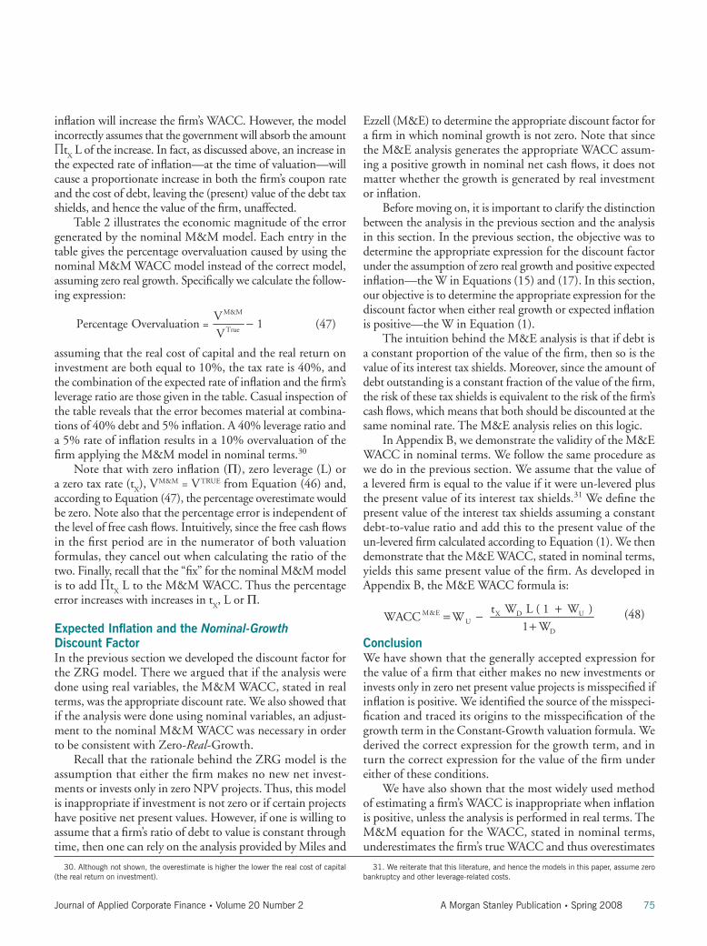
Table 2 illustrates the economic magnitude of the error generated by the nominal M&M model. Each entry in the table gives the percentage overvaluation caused by using the nominal M&M WACC model instead of the correct model, assuming zero real growth. Specifically we calculate the follow-ing expression:

(47)M&M

True

VPercentage Overvaluation = 1

V (47)

assuming that the real cost of capital and the real return on investment are both equal to 10%, the tax rate is 40%, and the combination of the expected rate of inflation and the firm’s leverage ratio are those given in the table. Casual inspection of the table reveals that the error becomes material at combina-tions of 40% debt and 5% inflation. A 40% leverage ratio and a 5% rate of inflation results in a 10% overvaluation of the firm applying the M&M model in nominal terms.30

Note that with zero inflation (Π), zero leverage (L) or a zero tax rate (t

X), VM&M = VTRUE from Equation (46) and,

according to Equation (47), the percentage overestimate would be zero. Note also that the percentage error is independent of the level of free cash flows. Intuitively, since the free cash flows in the first period are in the numerator of both valuation formulas, they cancel out when calculating the ratio of the two. Finally, recall that the “fix” for the nominal M&M model is to add ∏t

X L to the M&M WACC. Thus the percentage

error increases with increases in tX, L or Π.

Expected Inflation and the Nominal-Growth Discount Factor In the previous section we developed the discount factor for the ZRG model. There we argued that if the analysis were done using real variables, the M&M WACC, stated in real terms, was the appropriate discount rate. We also showed that if the analysis were done using nominal variables, an adjust-ment to the nominal M&M WACC was necessary in order to be consistent with Zero-Real-Growth.

Recall that the rationale behind the ZRG model is the assumption that either the firm makes no new net invest-ments or invests only in zero NPV projects. Thus, this model is inappropriate if investment is not zero or if certain projects have positive net present values. However, if one is willing to assume that a firm’s ratio of debt to value is constant through time, then one can rely on the analysis provided by Miles and

Ezzell (M&E) to determine the appropriate discount factor for a firm in which nominal growth is not zero. Note that since the M&E analysis generates the appropriate WACC assum-ing a positive growth in nominal net cash flows, it does not matter whether the growth is generated by real investment or inflation.

Before moving on, it is important to clarify the distinction between the analysis in the previous section and the analysis in this section. In the previous section, the objective was to determine the appropriate expression for the discount factor under the assumption of zero real growth and positive expected inflation—the W in Equations (15) and (17). In this section, our objective is to determine the appropriate expression for the discount factor when either real growth or expected inflation is positive—the W in Equation (1).

The intuition behind the M&E analysis is that if debt is a constant proportion of the value of the firm, then so is the value of its interest tax shields. Moreover, since the amount of debt outstanding is a constant fraction of the value of the firm, the risk of these tax shields is equivalent to the risk of the firm’s cash flows, which means that both should be discounted at the same nominal rate. The M&E analysis relies on this logic.

In Appendix B, we demonstrate the validity of the M&E WACC in nominal terms. We follow the same procedure as we do in the previous section. We assume that the value of a levered firm is equal to the value if it were un-levered plus the present value of its interest tax shields.31 We define the present value of the interest tax shields assuming a constant debt-to-value ratio and add this to the present value of the un-levered firm calculated according to Equation (1). We then demonstrate that the M&E WACC, stated in nominal terms, yields this same present value of the firm. As developed in Appendix B, the M&E WACC formula is:

(48)t W L ( 1 W )M&E U

D1 W (48) U

X DWACC W

Conclusion We have shown that the generally accepted expression for the value of a firm that either makes no new investments or invests only in zero net present value projects is misspecified if inflation is positive. We identified the source of the misspeci-fication and traced its origins to the misspecification of the growth term in the Constant-Growth valuation formula. We derived the correct expression for the growth term, and in turn the correct expression for the value of the firm under either of these conditions.

We have also shown that the most widely used method of estimating a firm’s WACC is inappropriate when inflation is positive, unless the analysis is performed in real terms. The M&M equation for the WACC, stated in nominal terms, underestimates the firm’s true WACC and thus overestimates

30. Although not shown, the overestimate is higher the lower the real cost of capital (the real return on investment).

31. We reiterate that this literature, and hence the models in this paper, assume zero bankruptcy and other leverage-related costs.


its value. The M&M model can be expressed in nominal terms provided the real WACC is calculated first according to the M&M formula, and then the nominal WACC is calculated from the Fisher Equation. Alternatively, the nominal version of the M&M model can be found by first calculating the WACC in nominal terms, and then adding the correction factor ∏t

X L. Finally, we show that if the ratio of the firm’s debt

to value remains constant over time, then the nominal WACC according to Miles & Ezzell is appropriate and requires no adjustment.

michael bradley is the F.M. Kirby Professor of Investment Bank-

ing, Fuqua School of Business and Professor of Law, Duke University

([email protected]).

gregg jarrell is Professor of Finance and Economics, William E.

Simon Graduate School of Business Administration, University of Roch-

ester ([email protected]).

ReferencesBrealey, R.A., S. C. Myers and F. Allen, Principles of Corpo-

rate Finance, 8th ed. (New York: McGraw-Hill, 2006).Benninga, Simon and Oded Sarig, Corporate Finance: A

Valuation Approach (McGraw-Hill, 1997).Bodie, Z. and R. Merton, Finance (New Jersey: Prentice

Hall, 2000).Copeland, T., T. Koller and J. Murin, Valuation, 2nd ed.

(New York: John Wiley & Sons,1994).Cornell, B., Corporate Valuation (New York: Irwin,

1993).Fisher, I., The Theory of Interest (New York: Augustus M.

Kelley, Publishers, 1965). Reprinted from the 1930 edition.Martin, J., J.W. Petty, A. Keown, D. Scott, Basic Financial

Management, 5th ed. (New Jersey: Prentice Hall, 1991).Miles, J. and J. Ezzell, The Weighted Cost of Capital,

Perfect Capital Markets, and Project Life: A Clarification, Journal of Financial and Quantitative Analysis 15 (1980), pp. 719-730.

Modigliani, F. and M. H. Miller, “Corporate Income Taxes and the Cost of Capital: A Correction,” American Economic Review, Vol. 53: 433-443 (June 1963).

Myers, S., “Determinants of Corporate Borrowing,” Journal of Financial Economics 5 (1977) 147-175.

Rao, R., Financial Management, (Ohio: Southwestern College Publishing, 1995).

Rappaport, A., Creating Shareholder Value, 2nd ed. (New York: The Free Press, 1998).

Ross, S.A., R. Westerfield and J. Jaffe, Corporate Finance, 3rd Edition, (Illinois: Irwin, 1993.

Shapiro, A. and S. Balbirer, Modern Corporate Finance (New Jersey: Prentice-Hall, 2000).

Stewart III, G.B., The Quest for Value (USA: Harper Business, 1991).

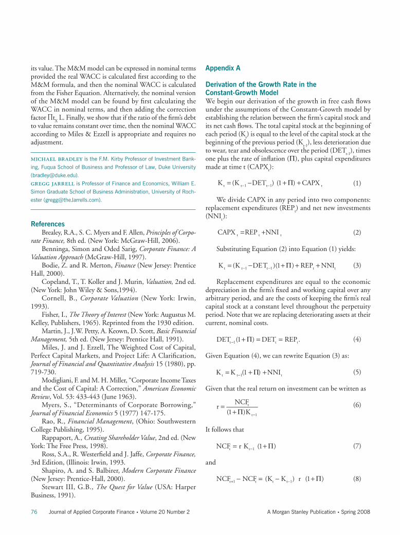
Appendix A Derivation of the Growth Rate in the Constant-Growth ModelWe begin our derivation of the growth in free cash flows under the assumptions of the Constant-Growth model by establishing the relation between the firm’s capital stock and its net cash flows. The total capital stock at the beginning of each period (K

t) is equal to the level of the capital stock at the

beginning of the previous period (Kt-1

), less deterioration due to wear, tear and obsolescence over the period (DET

t-1), times

one plus the rate of inflation (Π), plus capital expenditures made at time t (CAPX

t):

(1)CA

t t tCAPX REP NNI )2(

t t 1K (K DE (3)

t 1 t t(1 ) DET REP . )4(

t t 1 t 1 tK (K DET ) (1 ) PX (1)

t 1 t tT )(1 ) REP NNI

DET

t t 1 tK K (1 ) NNI )5(

We divide CAPX in any period into two components: replacement expenditures (REP

t) and net new investments

(NNIt):

CA


t t 1K (K DE (3)

t 1 t t(1 ) DET REP . )4(

t t 1 t 1 tK (K DET ) (1 ) PX (1)


DET

t t 1 tK K (1 ) NNI )5(

(2)

Substituting Equation (2) into Equation (1) yields:

CA


t t 1K (K DE (3)

t 1 t t(1 ) DET REP . )4(

t t 1 t 1 tK (K DET ) (1 ) PX (1)


DET

t t 1 tK K (1 ) NNI )5(

(3)

Replacement expenditures are equal to the economic depreciation in the firm’s fixed and working capital over any arbitrary period, and are the costs of keeping the firm’s real capital stock at a constant level throughout the perpetuity period. Note that we are replacing deteriorating assets at their current, nominal costs.

CA


t t 1K (K DE (3)

t 1 t t(1 ) DET REP . )4(

t t 1 t 1 tK (K DET ) (1 ) PX (1)


DET

t t 1 tK K (1 ) NNI )5(

(4)

Given Equation (4), we can rewrite Equation (3) as:

(5)

CA


t t 1K (K DE (3)

t 1 t t(1 ) DET REP . )4(

t t 1 t 1 tK (K DET ) (1 ) PX (1)


DET

t t 1 tK K (1 ) NNI )5(

Given that the real return on investment can be written as

(6) t

t 1

NCFr

(1 )K

t t 1NCF r K (1 )

t 1 t t t 1NCF NCF (K K ) r (1 ) (8)

It follows that

(7)

t

t 1

NCFr

(1 )K

t t 1NCF r K (1 )

t 1 t t t 1NCF NCF (K K ) r (1 ) (8)

and

(8)

t

t 1

NCFr

(1 )K

t t 1NCF r K (1 )

t 1 t t t 1NCF NCF (K K ) r (1 ) (8)


Substituting Kt from Equation (5) into Equation (8) yields:

(9)

Note that the first and last variables in the bracketed term on the RHS of Equation (9) are the same – Kt-1 . Expanding Equation (9) and canceling out the Kt-1 terms yields:

(10)t 1 t t 1 tNCF NCF [K NNI ] r (1 ) (10)

Dividing Equation (10) by NCFt defines the growth in NCF and, since FCF

t = NCF

t (1–k), the growth in FCF as well:

t 1 t 1

tt

NCF NCF FCF FG

NCF FCF t tCF

(11)

(12)t 1 t

t 1 t 1

K r (1 ) NNI r (1 )G

K r (1 ) K r (1 )

Recall that

(13)t tNNI NNIk

t t 1NCF K r(1 )

Substituting (13) into (12) yields:

G + k r (1+ ) = + kr + k r (14)

Define g as real growth in free cash flows. Since G = g when Π = 0, it follows from Equation (14) that:

g = kr (15)

Equation (15) states that the real growth in FCF is equal to the plowback ratio times the real return on investment. To obtain the equation for nominal growth (G) in terms of nominal returns (R) and inflation (Π) add the quantity (+ kΠ – kΠ) to Equation (14)

G = + kr + kr + k - k (16)

G = k ( r + +r ) + ( 1 - k ) (17)

G = k R + ( 1 - k ) )81(

(16)

collect terms,G = + kr + kr + k - k (16)

G = k ( r + +r ) + ( 1 - k ) (17)

G = k R + ( 1 - k ) )81(

(17)

and substitute R = r + Π + r Π from the Fisher Equation for the nominal return to investment:

G = + kr + kr + k - k (16)

G = k ( r + +r ) + ( 1 - k ) (17)

G = k R + ( 1 - k ) )81( (18)

This is the general expression for the nominal growth in free cash flows.

Appendix B

WACC According to Miles and Ezzell The WACC methodology developed by Miles and Ezzell (M&E) does hold in nominal terms. This model assumes that the ratio of debt to value remains constant through time. Thus, if the nominal value of the firm grows with inflation, so does the amount of debt outstanding and, as a result, the per period interest tax shield. All else equal, the value of a levered firm (the market value of its outstanding securities) is positively related to the rate of inflation. The value of the firm is not inflation neutral under the M&E model. Since the value of the firm’s tax shields increases with inflation, the M&E model is not correct if the parameters are stated in real terms.

According to the M&E assumptions, the present value of the firm’s interest tax shield is equal to:

(19)t-1

X D Lt-1

t 1 D U

t W L V ( 1 G )PVITS

( 1 W ) ( 1 W )

The numerator of Equation (19) is the interest tax shield in period t – the tax rate times the interest rate times the debt to value ratio times the value of the firm at the beginning of the first period times the appropriate growth factor. Note that the interest tax shield is based on the beginning value of the firm. The denominator of Equation (19) reflects the fact that under the M&E assumptions, the amount of debt in the first period is known and therefore the interest tax shield is discounted at the rate on debt, W

D. Thereafter, the amount

of debt outstanding depends on the value of the firm. Since L is constant, the firm issues debt when the value of the firm rises and retires debt when the market value falls. Thus, the size of the interest tax shield rises and falls with the value of the firm. Consequently, the interest tax shield is as risky as the firm itself, which accounts for discounting the per period tax shield at the un-levered cost of capital, W

U, from period

t = 2 onward. For purposes that will become clear shortly, we isolate the

first year’s tax shield

(20)

PVITS

t 2 ( 1 W ) ( 1 W )D Ut-1

t-1X D Lt W L V ( 1 G )

X D Lt W L V 1 WD

where, VL is the value of the levered firm in period 0. Adjust-

ing the time subscripts in the second term:


(21)x D L

D

t W L VPVITS 1 W

tx D L

tt 1 UD

t W L V ( 1 G ) ( 1 W ) ( 1 W )

Define Q as:

(22)

Substituting (22) into (21) and applying the formula for the value of a growing perpetuity:

(23)

Recall that the value of a levered firm is equal to the value of an un-levered firm plus the present value of interest tax shields (PVITS):

(24)UL U

U

Q (1 W )V V

W - G U

L UU

Q (1 W )V V

W - G

We now demonstrate that the WACC model developed by M&E yields this same expression. Under the M&E assump-tions, the firm’s nominal cost of equity is:

(25)

Substituting Equation 25 into the weighted into the weighted average cost of capital formula:

(26)

yields:

(27)

Substituting Q yields:

(28)

Substituting WACCM&E into the denominator of the basic valuation formula yields:

(29)

Multiplying through by the denominator yields:

(30)

(31)

(32)

Dividing through by ( WU – G ) yields:

(33)

(34)

Thus, Equation (29) equals Equation (24), which implies that the M&E model is correct in nominal terms.

Note that since the M&E model assumes a constant ratio of debt to equity, the firm’s debt, and hence its tax shields, will increase at the rate of inflation, and the M&E model, stated in real terms, cannot account for this increase in value.


Journal of Applied Corporate Finance (ISSN 1078-1196 [print], ISSN 1745-6622 [online]) is published quarterly, on behalf of Morgan Stanley by Blackwell Publishing, with offices at 350 Main Street, Malden, MA 02148, USA, and PO Box 1354, 9600 Garsington Road, Oxford OX4 2XG, UK. Call US: (800) 835-6770, UK: +44 1865 778315; fax US: (781) 388-8232, UK: +44 1865 471775.

information for subscribers For new orders, renewals, sample copy requests, claims, changes of address, and all other subscription correspondence, please contact the Customer Service Department at your nearest Blackwell office (see above) or e-mail [email protected].

subscription Rates for Volume 20 (four issues) Institutional Premium Rate* The Americas† $377, Rest of World £231; Commercial Company Premium Rate, The Americas $504, Rest of World £307; Individual Rate, The Ameri-cas $100, Rest of World £56, €84‡; Students** The Americas $35, Rest of World £20, €30.

*The Premium institutional price includes online access to current content and all online back files to January 1st 1997, where available.

†Customers in Canada should add 6% GST or provide evidence of entitlement to exemption. ‡Customers in the UK should add VAT at 6%; customers in the EU should also add VAT at 6%, or provide a VAT registration number or evidence of entitlement to exemption.

**Students must present a copy of their student ID card to receive this rate.

For more information about Blackwell Publishing journals, including online access information, terms and conditions, and other pricing options, please visit www.blackwellpublishing.com or contact your nearest Customer Service Department.

Back issues Back issues are available from the publisher at the current single- issue rate.

Mailing Journal of Applied Corporate Finance is mailed Standard Rate. Mail-ing to rest of world by DHL Smart & Global Mail. Canadian mail is sent by Canadian publications mail agreement number 40573520. postmaster Send all address changes to Journal of Applied Corporate Finance, Blackwell Publishing Inc., Journals Subscription Department, 350 Main St., Malden, MA 02148-5020.

Journal of Applied Corporate Finance is available online through Synergy, Blackwell’s online journal service, which allows you to:• Browse tables of contents and abstracts from over 290 professional,

science, social science, and medical journals• Create your own Personal Homepage from which you can access your

personal subscriptions, set up e-mail table of contents alerts, and run saved searches

• Perform detailed searches across our database of titles and save the search criteria for future use

• Link to and from bibliographic databases such as ISI.Sign up for free today at http://www.blackwell-synergy.com.

Disclaimer The Publisher, Morgan Stanley, its affiliates, and the Editor cannot be held responsible for errors or any consequences arising from the use of information contained in this journal. The views and opinions expressed in this journal do not necessarily represent those of the Publisher, Morgan Stan-ley, its affiliates, and Editor, neither does the publication of advertisements constitute any endorsement by the Publisher, Morgan Stanley, its affiliates, and Editor of the products advertised. No person should purchase or sell any security or asset in reliance on any information in this journal.

Morgan Stanley is a full service financial services company active in the securities, investment management, and credit services businesses. Morgan Stanley may have and may seek to have business relationships with any person or company named in this journal.

Copyright © 2008 Morgan Stanley. All rights reserved. No part of this publi-cation may be reproduced, stored, or transmitted in whole or part in any form or by any means without the prior permission in writing from the copyright holder. Authorization to photocopy items for internal or personal use or for the internal or personal use of specific clients is granted by the copyright holder for libraries and other users of the Copyright Clearance Center (CCC), 222 Rosewood Drive, Danvers, MA 01923, USA (www.copyright.com), pro-vided the appropriate fee is paid directly to the CCC. This consent does not extend to other kinds of copying, such as copying for general distribution for advertising or promotional purposes, for creating new collective works, or for resale. Institutions with a paid subscription to this journal may make photocopies for teaching purposes and academic course-packs free of charge provided such copies are not resold. Special requests should be addressed to Blackwell Publishing at: [email protected].

Documents

Expected Inflation and the Constant-Growth Valuation Model