Expectations and Macro-Housing Interactions in

a Small Open Economy: Evidence from Korea∗

Fabio MILANI

University of California, Irvine

Sung Ho PARK

Bank of Korea

Abstract

This paper studies the interaction between the housing sector and the macroeconomic envi-ronment in Korea. Besides serving as a typical small open economy, Korea provides an inter-esting laboratory case, since the country was subject to various housing-cycle phases over thesample, and its policymakers implemented active policies to stabilize the housing market.

We present a microfounded open-economy model extended to incorporate a housing sector.The model is estimated using Bayesian methods and a large set of observables.

We highlight the role of assumptions about house-price expectations on economic dynamics.In the benchmark case of rational expectations, the spillovers from housing to macro variables aremodest. House prices are largely driven by sector-specific demand and supply shocks. Businesscycle fluctuations are mostly driven by open-economy shocks.

When the assumption of rational expectations is relaxed in favor of extrapolative expec-tations, however, the impact of the housing sector increases. Macroeconomic spillovers fromthe housing market become more important, with housing shocks accounting for up to twentypercent of fluctuations in the broader economy.

Keywords: Housing Market-Macroeconomy Nexus, House Prices, Non-Rational Expectations,

Macroprudential Policies, Household Credit, Small Open Economy Model, Korea’s Economy.

JEL classification: E03, E32, E58, F41, R30.

[The views expressed herein are those of authors and do not necessarily reflect the official views

of the Bank of Korea. When reporting or citing this paper, the authors’ name should always be

explicitly stated.]

∗We would like to thank seminar participants at the Bank of Korea for comments. Professor Milani acknowledgesand is grateful for the financial support provided by the Bank of Korea regarding this research project.

1 Introduction

The housing market in Korea has often been at the center of policymakers’ attention and

discussions in recent years. The country has experienced a protracted run-up of house prices,

followed by their collapse, in the 1990s. More recently, real house prices have been remarkably

stable, and seemingly unresponsive to economic conditions; construction activity, on the other hand,

has been through boom and bust phases in the same period. Observers of the country’s economic

situation are particularly worried about persistent increases in household credit, in large part

used to finance housing expenses. While the same phenomenon has happened in many countries,

Korea’s example is peculiar in that it didn’t suffer any deleveraging in the aftermath of the 2007-

2009 financial crisis. Moreover, the level of household indebtedness has risen to become one of the

largest among developed countries.

In this paper, our main aim is to shed more light on the interdependence between the housing

market and the real economy in Korea. The country provides an almost ideal laboratory to study

the housing-macro nexus in a small and considerably open economy. Moreover, Korea’s example is

particularly noteworthy because policymakers, unlike their counterparts in other countries, have a

long history of implementing macroprudential policies to either stabilize or stimulate the real-estate

sector. They have repeatedly used limits on loan-to-value ratios, as well as debt-to-income limits.

We adopt a microfounded model that incorporates a number of features that have been found

essential to match the empirical properties of macroeconomic dynamics in small open economies.

The model includes endogenous sources of persistence, such as habit formation, adjustment costs in

investment, and price indexation; it implies imperfect exchange-rate pass-through and it assumes

incomplete international financial markets, an assumption that gives rise to deviations from the

uncovered interest parity condition. The small open economy model is extended to include a

housing sector, following the seminal work by Iacoviello (2005) and Iacoviello and Neri (2010).

Housing services provide direct utility to households. Houses can also serve as collateral in the

borrowing contracts in the model. The economy is populated by two groups of households, which

differ in their degree of patience, i.e. the rates at which they discount the future. Heterogeneity in

patience motivates the desire for borrowing and lending in the model. In contrast to many papers

in the housing market-macroeconomic literature, we do not assume the housing stock to be fixed (a

feature that amplifies the effects of house price movements), but we allow for housing production

and investment, with both broad and sector-specific technology shocks (as in Iacoviello and Neri

1

(2010), but differently from Iacoviello (2005)).

We estimate the model using full-information Bayesian methods. The estimation attempts to

match a wide set of observable variables, covering domestic indicators, housing and credit variables,

and open-economy and foreign variables.

1.1 Main Findings

Our results shed light on the strength of the nexus between housing, the credit market, and the

broader macroeconomy, in an environment that is deeply influenced by global economic conditions.

We find that house prices are mostly explained by housing-specific demand and supply shocks.

They are only in modest part driven by non-housing factors.

Housing and credit shocks spill over to the rest of the economy, but, at least based on the

benchmark model under rational expectations, the magnitude of macroeconomic spillovers is rather

contained: these shocks explain 5% of consumption fluctuations, 10% of investment, and 3% of GDP

fluctuations. The main determinants of macroeconomic dynamics, at business cycle frequencies,

are shocks that are related to the open-economy nature of the country (e.g., exchange rate, terms

of trade, import-price, as well as purely foreign shocks).

We then study the potential impact of two measures that are meant to capture the macropruden-

tial policies adopted during the sample in Korea: limits on loan-to-value ratios and debt-to-income

limits. Our results show that these policies can be effective. Lower limits operate to reduce the

sensitivity of house prices and credit to housing and credit shocks. Importantly, these targeted poli-

cies do so without causing broader recessionary effects on the macroeconomy, as it would happen

through the use of conventional monetary policies.

We particularly emphasize the importance of expectation formation mechanisms for the trans-

mission of housing market and credit shocks. We start by modeling expectations as formed accord-

ing to the rational expectations hypothesis. We then consider deviations from rational expectations,

initially in the formation of house-price expectations only. Such expectations are allowed to be non-

rational, extrapolative, and formed from a simple adaptive learning model. Economic agents just

use information from past house prices to extrapolate their future direction. When this adaptive

learning specification is estimated for house prices, it uncovers house-price beliefs that are quite

persistent, and characterized by a period, preceding the crisis, when beliefs become potentially

unstable. For the reminder of the sample, the inferred beliefs are more stable, but very persistent,

leading to sluggish house-price expectations.

When house-price expectations are formed in a non-rational fashion, the impact of housing and

2

credit conditions on the rest of the economy is amplified. Housing demand and credit shocks lead

to long and persistent adjustments in house prices and construction investment. They lead to boom

and bust cycles in aggregate investment and output. The portion of macroeconomic fluctuations in

the country due to shocks that have their origin in the housing sector also rises considerably, from

three percent to up to slightly more than twenty percent. The results are similar when we allow

extrapolative expectations to be more pervasive, by affecting every expectation in the model, not

just those related to house prices.

1.2 Related Literature

Iacoviello (2005) and Iacoviello and Neri (2010) are seminal papers that introduce a housing sector

in a general equilibrium macroeconomic model; the latter estimates a closed-economy model to fit

U.S. data. This paper builds on their work to study the interaction of housing and the broader

macroeconomy in a small and considerably open economy. Our scope is, therefore, similar to that

in the papers by Christensen et al. (2016), Aoki et al. (2004), Funke and Patz (2013), Ng and Feng

(2016), and Robinson and Robson (2012), among others.

Our results show that fluctuations in Korea are driven to a large extent by open-economy

shocks. The findings are consistent with those in Milani and Park (2015), who estimate the effects

of globalization on the Korean economy (but abstracting from a housing sector).

We stress the role of macroprudential regulation and the importance of assumptions on the

formation of expectations. The impact of macroprudential policies have been studied in Igan

and Kang (2011), who also use the Korean experience as the example of choice. They exploit

disaggregated household-level data and find that loan-to-value and debt-to-income limits lead to

declines in house prices, reduced real-estate transaction activity, and help curb expectations. Hahm

et al. (2011) provide a broad discussion on the benefits of macroprudential supervision and argue

that it can be especially needed and effective in open emerging economies.

Finally, a number of empirical studies have dealt with the relationship between housing and

macroeconomic variables in Korea, using different techniques (e.g., Kim (2004), Lee and Song

(2015)). Lee and Song (2015) estimate a closed-economy model on Korean data, with a housing

sector modeled as in Iacoviello and Neri (2010). Our paper uses a small open economy framework,

which is important for Korea, since, as we show, the vast majority of fluctuations are driven by

open-economy shocks. Moreover, we uncover a key role for expectations: deviations from fully-

rational expectations in the housing market may lead to a magnification of the spillovers from the

housing market to the real economy.

3

2 Model

We present a small open economy model that is extended to capture interactions between the real

economy and the housing sector. Housing is modeled borrowing features from Iacoviello (2005)

and Iacoviello and Neri (2010). Housing provides utility to households directly, but it also serves

as collateral. A share of households in the model decide to access credit and they are allowed to

borrow up the the value of their collateral. Through this channel, fluctuations in house prices affect

the value of collateral and they may have potentially sizable effects on aggregate consumption and

on the real economy. On the supply side, the housing sector employs dedicated labor, capital, and

land, in the production of new housing units.

The open economy features in the model are similar to those introduced by Galı and Monacelli

(2005) and Monacelli (2005). Households consume a basket of domestically-produced and imported

goods. International financial markets are assumed to be incomplete: the unconstrained households

who fully participate in financial markets can purchase domestic and foreign bonds. Domestic

producers and importers operate under monopolistic competition and have sticky prices. The model

contains features that have been shown critical to match the empirical evidence, such as habit

formation, backward-looking indexation, incomplete exchange-rate pass-through, and deviations

from the uncovered interest parity condition. Besides being exposed to a wide variety of domestic

shocks, the home economy is affected by external shocks to foreign output, inflation, and interest

rates. Galı and Monacelli (2005) and Monacelli (2005)’s models are extended here to incorporate

a housing sector and to include investment decisions and capital accumulation.1

The majority of papers considerably simplify housing production, by either assuming that the

supply of housing is fixed (thus magnifying the response of house prices to shocks) or by considering

housing as an intermediate good that is transformed subject to adjustment costs (Aoki et al. (2004),

Christensen et al. (2016)). Here, we follow instead Iacoviello and Neri (2010) and Robinson and

Robson (2012) in modeling housing production more extensively. Houses are produced in a separate

housing sector, employing sector-specific inputs and technology. This modification allows us to

attempt to explain the behavior of residential investment as well, besides housing prices. Our

model is, therefore, similar to Robinson and Robson (2012), with some simplifications.2

1Small-open economy DSGE models have been taken to the data by Justiniano and Preston (2010), Kam et al.(2009), among others; Milani and Park (2015) estimate a similar model, but without a housing sector, to study theconsequences of globalization on the Korean economy.

2We adopt a simplified labor market (we drop the assumption of imperfect substitutability between labor betweensectors, among other things), a cashless economy, and do not consider intermediate inputs in housing production.We experiment with extrapolative, rather than rational, expectations, later in the paper.

4

2.1 Heterogeneous Households

The economy is composed of two heterogeneous groups of households (with each group composed

of a continuum of agents in the unit interval), who differ in their degrees of impatience. ‘Patient’

households discount future utility at a discount factor βs, while relatively ‘impatient’ households

have a discount factor βb, with βb < βs. Such difference in patience is a key feature in the model

to motivate borrowing and lending, with patient agents becoming net savers in equilibrium, and

impatient agents becoming net borrowers.

Both groups of households maximize the same utility function

maxE0

∞∑

t=0

βtj

[ζt log (Cj,t − ηCj,t−1) + Jt logHj,t −Ψ

N1+ψj,t

1 + ψ

]. (1)

where j = s, b indexes household types (with s standing for patient/savers and b for impa-

tient/borrowers). Households receive utility from consumption Cj,t, housing services Hj,t, and

disutility from hours of labor Nj,t = (Nj,c,t +Nj,h,t), where the further subscript c and h denote

work in the intermediate goods or consumption sector, and work in the housing sector, respectively.

Consumers’ preferences are characterized by habit formation, the strength of which is measured

by the parameter η. Housing services are typically assumed as proportional to the housing stock.

The term ζt represents an aggregate preference shock, while Jt is an housing preference disturbance

(both disturbances are common across the two types of agents). The housing disturbance captures

the role of exogenous shifts in housing demand, for example driven by population growth, or shifts

in the taste for homeownership. The parameter ψ denotes the inverse of the Frisch elasticity of labor

supply. The households’ consumption basket is a Dixit-Stiglitz aggregate of domestically-produced

and imported consumption goods:

Ct =

[(1− γ)1/σC

σ−1

σ

H,t + γ1/σCσ−1

σ

F,t

] σσ−1

, (2)

where 0 ≤ γ ≤ 1 measures the share of imported foreign goods in the consumption basket (typically

interpreted in the international macro literature as the degree of openness of the home economy)

and σ > 0 denotes the elasticity of substitution across domestic and foreign goods. Aggregate CH,t

and CF,t are given by CH,t =[∫ 1

0 CH,t(j)ε−1

ε dj] ε

ε−1

and CF,t =[∫ 1

0 CF,t(j)ε−1

ε dj] ε

ε−1

. The demand

functions for domestic and foreign consumption goods are given by CH,t = (1−γ)(PH,t/Pt)−σCt and

CF,t = γ(PF,t/Pt)−σCt, where PH,t and PF,t denote price indexes for domestic and foreign-produced

goods. Finally, the aggregate price level Pt can be expressed as Pt =[(1− γ)P 1−σ

H,t + γP 1−σF,t

] 1

1−σ.

5

2.1.1 Patient Households/Savers

Patient households are allowed to invest in housing and in capital used both by intermediate-goods

firms and by firms in the construction sector. They supply labor to both sectors. They can also

invest in an internationally-traded bond. Patient households, therefore, maximize (1) subject to

the budget constraint

Cs,t +PH,tPt

It +PH,tPt

Iht +Qht IHt +Rt−1

πtBs,t−1 + ΞtB

∗

t = Bs,t +R∗

t−1Φt(NFAt)Ξt

π∗tB∗

t−1+

+Ws,tNs,t +PH,tPt

rktKt−1 + rhtKht−1 +Πs,t + Tt, (3)

where Bt denotes domestic bond holdings, B∗

t denotes holdings of foreign (one-period) bonds,

It, Iht , Kt−1, and Kh

t−1 denote non-residential investment and capital in the business and in the

construction sector, IHt denotes residential investment, Qht denotes the real house price, Rt denotes

the domestic nominal interest rate,Wt the nominal wage, πt and π∗

t denote the domestic and foreign

inflation rates, rkt and rht denote returns on different types of capital, Πt denotes profit distributions,

and Tt lump-sum taxes or transfers. The variables It, Iht , Kt, B

∗

t have no s subscript given that

they refer only to savers, and not borrowers, in the model. The yield on foreign bonds is a function

of fluctuations in the nominal exchange rate Ξt, of the foreign interest rate R∗

t−1, and it is subject

to a risk-premium Φt:

Φt = exp [−χ(NFAt + φt)] (4)

NFAt =Ξt−1B

∗

t−1

Y Pt−1. (5)

The risk-premium evolves as a function of the country’s net financial asset positionNFAt (expressed

as a fraction of steady-state output Y ) and may be affected by an exogenous disturbance φt.3 The

parameter χ governs the sensitivity of the risk-premium to the country’s international financial

position. Capital in the consumption goods sector, housing-sector capital, and the housing stock

evolve as

Kt = (1− δ)Kt−1 + µt

[1− S

(ItIt−1

)]It (6)

KHt = (1− δkh)KH

t−1 +

[1− S

(IHtIHt−1

)]IHt (7)

Hj,t = (1− δh)Hj,t−1 + IHj,t. (8)

3This is a common assumption in open economy models; see, for example, Schmitt-Grohe and Uribe (2003).

6

The evolution of capital is subject to adjustment costs as in Christiano et al. (2005). We allow

for investment-specific technology disturbances µt to affect the transformation of investment into

capital.4 The rate of depreciations in the different sectors are denoted by δ, δkh, and δh.

The first-order conditions related to the saving, housing, borrowing, and labor choices, lead to

the following equilibrium conditions

ζt(Cs,t − ηCs,t−1)

= βsRtEt

[ζt+1

(Cs,t+1 − ηCs,t) πt+1

](9)

JtHs,t

=Qht ζt

Cs,t − ηCs,t−1− βs(1− δh)Et

[Qht+1ζt+1

Cs,t+1 − ηCs,t

](10)

Ws,t = ΨNψs,t

(Cs,t − ηCs,t−1)

ζt. (11)

The first-order condition related to international bond holdings implies the following no-arbitrage

relation

Et

[(R∗

t

Rt)(πt+1

π∗t+1

)(Ξt+1

Ξt)Φt+1(NFAt+1)

]= 0, (12)

which would typically restrict the differential between domestic and foreign interest rates to equal

the expected depreciation of the domestic currency. In our model, however, given the assumption

of incomplete markets, there can be a wedge in the relation, given by the country’s risk-premium,

which is driven both by endogenous factors and by the exogenous risk-premium disturbance φt.

Finally, the real exchange rate and the terms of trade are defined as Qt = ΞtP ∗

t

Ptand τt =

PF,t

PH,t.

2.1.2 Impatient Households/Borrowers

Relatively impatient households maximize their lifetime utility subject to the sequence of budget

constraints

Cb,t +Qht IHb,t = Bb,t −Rt−1

πtBb,t−1 +Wb,tNb,t +Πb,t, (13)

and, in addition, to the borrowing constraint

Bb,t ≤ mMtEt

[Qht+1Hb,tπt+1

Rt

]. (14)

The term Bb,t denotes the amount of borrowing by impatient households, m represents the steady-

state loan-to-value ratio, and Mt represents an exogenous disturbance to the LTV ratio. The

latter can be viewed as a proxy for collateral evaluation, a proxy for default risk, a measure of

4For simplicity, we assume investment-specific technology shocks in the business sector, but not in housing. Theassumption is that the kind of technological advances in the production of new equipment, emphasized in Greenwoodet al. (1997), may have been important in the business sector, but less crucial in the construction sector.

7

the restrictiveness of loans, or more broadly as a ‘credit’ shock. Impatient agents do not invest in

capital or in international assets. The first-order conditions are as follows

ζt(Cb,t − ηCb,t−1)

= βbRtEt

[ζt+1

(Cb,t+1 − ηCb,t)πt+1

]+ Λb,tRt (15)

JtHb,t

=Qht ζt

Cb,t − ηCb,t−1

−βb(1− δh)Et

[Qht+1ζt+1

Cb,t+1 − ηCb,t

]− Λb,tmMtEt

[Qht+1πt+1

](16)

Wb,t = ΨNψb,t

(Cb,t − ηCb,t−1)

ζt(17)

where Λb,t denotes the Lagrange multiplier associated to the collateral constraint.

2.2 Firms

2.2.1 Domestic Producers

Domestic firms, indexed by i, produce intermediate goods Yt(i) using capital and labor by patient

and impatient households, according to a Cobb-Douglas production function:

Yt(i) = AtKαt−1

(Ns,c,t(i)

ǫNb,c,t(i)1−ǫ)1−α

(18)

The parameter α denotes the capital share and ǫ denotes the share of labor income for patient

households. The term At represents a neutral technology disturbance.

Firms operate in a monopolistically-competitive market. They set prices a la Calvo: a fraction

1− θH of firms can set prices optimally in a given period; the remaining fraction θH is not allowed

to reoptimize its pricing plans and simply adjusts prices based on the past period’s inflation rate

πH,t−1, according to the indexation rule

log PH,t(j) = log PH,t−1(j) + γHπH,t−1, (19)

where 0 ≤ γH ≤ 1 denotes the degree of inflation indexation. Firms maximize profits subject

to the demand curve for their product. Optimization leads to a standard New Keynesian Phillips

curve (after log-linearization), where the current domestic inflation rate depends on past and future

expected inflation rates, on aggregate marginal costs, and on the price markup disturbance εpt :

πH,t =β

1 + βγHEtπH,t+1 +

γH1 + βγH

πH,t−1 +(1− βθp)(1− θp)

(1 + βγH)θpmct + εpt . (20)

8

2.2.2 Importers

Importers also operate under monopolistic competition. They purchase foreign goods at the price

PF,t = ΞtP∗

t . They differentiate the goods and set prices as a markup over marginal costs. Import

prices are sticky a la Calvo, with a probability 1−θF of resetting prices optimally in a given quarter.

With probability θF , firms simply update the prices according to the indexation rule

log PF,t(j) = logPF,t−1(j) + γFπF,t−1, (21)

where 0 ≤ γF ≤ 1 measures the extent of indexation.

In the spirit of Monacelli (2005), the law of one price holds at the docks, but the importing

firms’ pricing power leads to law of one price deviations in the short run and to imperfect exchange

rate pass-through. Importing firms maximize profits subject to the demand curve CF,T (j) =(PF,t(j)PF,T

(PF,T−1

PF,t−1

)γF )−εCF,T . The resulting law of motion for import-price inflation is as follow

πF,t =β

1 + βγFEtπF,t+1 +

γF1 + βγF

πF,t−1 +(1− βθF )(1− θF )

(1 + βγF )θF[rert − (1− γ)τt] + εipt , (22)

where εipt denotes a cost-push disturbance. Import inflation is driven by past inflation, expected

one-period-ahead inflation, and importers’ marginal costs, which are a function of the real exchange

rate rert and of the terms of trade τt. Aggregate CPI inflation is obtained as a weighted average

of domestic and foreign, import, inflation.

πt = (1− γ)πH,t + γπF,t. (23)

2.2.3 Housing Production

Firms in the housing sector add new units to the existing housing stock and operate under perfect

competition. They produce new housing units according to the production function

IHt = AtAhtK

h ǫht−1 L

ǫlt

(Ns,h,t(i)

νNb,h,t(i)1−ν)1−ǫh−ǫl (24)

where Aht is a sector-specific technology disturbance, Lt denotes land, and ǫh, ǫl, ν, denote the

respective elasticities. Land is assumed fixed in the short-run. Firms decide the investment level

IHt to maximize profits Πht , given by

maxΠht = Qht IHt −Ws,tNs,h,t −Wb,tNb,h,t − rhtKht−1 − rltLt, (25)

where rlt denotes the return on land.

9

2.3 Exports, Trade Balance, Value Added

Exports are modeled as

Xt =

(PH,tΞtP

∗

t

)−σ∗

Y ∗

t . (26)

The demand for exports is, therefore, isomorphic to the demand for domestic and imported goods,

with a potentially different elasticity of substitution σ∗. The trade balance is given by

Xt

Yt−

ΞtP∗

t

PH,t

CmtYt

= NFAt −R∗

t−1Φt(NFAt)Ξt/Ξt−1

πH,t

1

∆YtNFAt−1. (27)

We sum value added over the two sectors to obtain

GDPt =PH,tPt

Yt +Qht IHt. (28)

2.4 Monetary Policy

We assume that monetary policy in the home country is well approximated by the following Taylor

rule

Rt = ρRt−1 + (1− ρ)[ψππt + ψGDP∆GDPt + ψqh∆q

ht + ψe∆et

]+ εmp,t. (29)

The central bank is assumed to vary policy rates in reaction to movements in inflation and growth

in GDP, nominal exchange rates, and real house prices. While the situation in the housing market

doesn’t represent a stated policy target for the Bank of Korea, we still test whether there is a de

facto response to house prices, by including their growth rate in the rule. The term εmp,t accounts

for unsystematic deviations from the historical policy rule.5

2.5 Rest of the World

The foreign, or rest of the world, variables (y∗t , π∗

t , R∗

t ) that enter some of the main structural

equations are collected in the vector X∗

t and modeled as an unrestricted VAR(1):

X∗

t = X∗

t−1 +Ωε∗t . (30)

Foreign variables are computed as weighted averages as:

z∗t =

N∑

j=1

wz,jt zjt , (31)

5We assume here a constant response to exchange rates throughout the sample. In Milani and Park (2015), weallowed ψe to shift in value between the pre-1998 and post-1998 period. In this paper, the model with a constantcoefficient fits the data better and, hence, we report the results for this case in the estimation.

10

where the generic variable z = y, π,R, represents detrended output, inflation, and short-term

interest rate, respectively, of trading partner j, and where the weights wz,jt are given in each period

t by the sum of Korea’s imports and exports with country j, as a fraction of total Korean imports

and exports with the set of trading partners:

wz,jt =(Importsjt +Exportsjt)∑Ni=1(Imports

jt + Exportsjt)

. (32)

The same procedure has been used in Milani and Park (2015) to compute measures of global output,

inflation, and interest rates, relevant for Korea.6

2.6 Market Clearing and Log-Linearization

Aggregate consumption and housing are obtained as:

Ct = ωCb,t + (1− ω)Cs,t (33)

Ht = ωHb,t + (1− ω)Hs,t, (34)

where ω indicates the share of patient households in the economy. The model presented so far is

log-linearized around a non-stochastic steady-state. The log-linearized equations are reported in

their entirety in Appendix B.

3 Bayesian Estimation

3.1 Data

We use quarterly data for a sample starting in 1991:I and ending in 2014:IV. We estimate the

DSGE model to match fourteen observable series: real GDP, real consumption, real non-residential

(business) investment (with business investment defined as It + Iht in the model), real residential

investment, the CPI inflation rate, domestic inflation (from GDP deflator), the nominal effective

exchange rate, a short-term nominal interest rate (which serves as the policy instrument in the

model), the real house price index, real household credit, the terms of trade, and foreign output,

foreign inflation, and foreign interest rate. The data series are described in detail in Appendix A.

We detrend the real series using a band-pass filter (based on Christiano and Fitzgerald (2003)),

to extract fluctuations at business cycle frequencies.7 The terms of trade are detrended using a

6Here we focus on the country’s top ten trading partners (N = 10): the U.S., Japan, China, Germany, France,the Netherlands, the U.K., Switzerland, Singapore, and Hong Kong.

7Fukac and Pagan (2010) discuss some potential limitations that can arise from preliminary filtering of the data.

11

linear trend. Nominal exchange rates and interest rates are considered in deviations from a sample

mean (in both cases, we allow for a break in the mean before and after 1998).8

Figure 1 shows the observable series used in the estimation. The observables are related to the

corresponding variables in the model through the following observation equation:

Observablest = H0 +HYt, (35)

where H0 is a vector of zeros (for detrended variables) or sample means (for variables that are

demeaned as the exchange rate and interest rate), H is a selection matrix composed of zeros and

ones, and Yt = [gdpt, ct, it, iht , iht, πt, πH,t, et, Rt, q

ht , bb,t, τt, y

∗

t , π∗

t , R∗

t ]. The observable for residen-

tial investment corresponds to it + iht in the model. The coefficient in H related to et is 1/100 to

express the exchange rate in percentage deviation from steady-state.

3.2 Priors and Estimation Technique

Given the scale of the model, we fix some of the coefficients. As common in the literature, we fix

the discount factors: at 0.9925 for patient households (corresponding to a steady-state real interest

rate of 3%) and at 0.95 for impatient ones. The share of imports in the consumption basket γ is set

at 0.35 (based on Imports over GDP figures). The elasticities of substitution between domestic and

foreign produced goods and for exported goods are set at 0.5; the relatively low value is inspired

by our previous estimates in Milani and Park (2015). The Frisch elasticity of labor supply is set at

1. We assume a steady-state loan-to-value ratio in the middle of the 0.4-0.7 range that has been

often enforced in the sample, setting m = 0.55; j is set to obtain a value of the housing stock as a

fraction of GDP equal to 1.5;9 the ratio between household debt and GDP in steady-state, bbY, is

fixed at 0.8, the value observed on Korean data (source: IMF, Financial Soundness Indicators). We

similarly use actual data on net foreign debt to set the¯NFAY

ratio at 0.35 (source: Bank of Korea).

The parameters describing the input factor shares are similar to those in Iacoviello and Neri (2010)

and fixed as follows: α = 0.33, ǫ = 0.65, ǫh = 0.1, ǫl = 0.1, ν = 0.65. We assume depreciation

rates δ and δkh equal to 0.025. The depreciation rate for the housing stock is typically assumed

to be lower and set at 0.01 (e.g., Iacoviello and Neri (2010)). The elasticity of interest rates to

the country’s net foreign asset position χ is set at 0.001. Finally, the great-ratio coefficients are

8The exchange rate is transformed to correspond to the percentage deviation from steady state; the interest rateis expressed in deviation from steady state, since it’s already in percentage form.

9Kim (2004) provides data on the evolution of the total market capitalization of apartments versus Gross RegionalDomestic Product in the Seoul area (which, according to Igan and Kang (2011), accounts for 64% of total housingwealth in the country); the ratios fall between 100% and more than 200% over the sample.

12

convolutions of several steady-state parameters; we calibrate those to match their sample averages:

CY

= 0.55, IY

= 0.285, IH

Y= 0.065.

The priors for the coefficients that are estimated are presented in Table 1; in general, they are

similar to those used in other studies on the Korean economy (e.g., Lee and Song (2015)), other

small open economies (Ng and Feng (2016)), or closed-economies with a housing sector (Iacoviello

and Neri (2010)). The share of patient agents follows a Beta prior, with mean 0.65 and standard

deviation 0.05 (the same prior is used in Iacoviello and Neri (2010) and Lee and Song (2015)). We

assume Beta priors also for the habit formation coefficient, for indexation, for the Calvo parameters

(for those we assume a prior mean of 0.75, implying that prices are re-optimized on average once

a year), and for the autoregressive coefficients. The investment adjustment cost parameters have

a Gamma prior with mean 4 and standard deviation 1.5 (as in Smets and Wouters (2007)). For

monetary policy, we select a Normal prior for the inflation reaction coefficient (with mean 1.5 and

standard deviation 0.125) and Gamma priors for the reaction coefficients to GDP, exchange rate

depreciation, and house price growth. In the latter two cases, we adopt Gamma distributions

with mean and standard deviation values equal to each other, which imply probability masses

characterized by lower probabilities the farther the coefficient is from zero. We assume inverse-

gamma priors for the standard deviations of the structural disturbances. A subset of them has

lower prior mean consistent with our expectation that some of the shocks are expected to have

lower volatility. Finally, our priors for the foreign VAR mostly follow Milani and Park (2015).

The model is estimated using Bayesian methods. We generate draws using the Metropolis-

Hastings algorithm (the results are based on 600,000 draws), allowing the first 40% of draws to be

discarded as initial burn-in.

4 Empirical Results

4.1 Structural Parameter Estimates

Table 1 reports the posterior estimates for the model’s structural parameters, along with 95%

posterior probability intervals. The posterior mean estimate for ω indicates that slightly more

than two thirds of households in the economy can be interpreted as patient, while one third is

composed by impatient agents, or borrowers (the share is 0.79 in Iacoviello and Neri (2010) and

0.64 in Lee and Song (2015)). The economy is subject to substantial frictions: the degree of habit

formation η is estimated at 0.67; the adjustment costs in investment parameters are estimated

at comparable values across sectors, but somewhat larger for investment in the housing sector

13

(ϕ = 4.49, ϕkh = 5.39); Lee and Song (2015) also find larger adjustments costs for capital in

the construction sector. The indexation coefficients are estimated at 0.48 for domestic firms and

0.44 for importing firms. Prices are more rigid in the importing sector, with a Calvo parameter

estimated at 0.85.

The estimates for the Taylor rule fall around conventional values. Interestingly, the evidence

suggests that the central bank has considered house prices to some extent in the formulation of

monetary policy (ρ = 0.65, ψπ = 1.54, ψgdp = 0.08, ψe = 0.01, ψqh = 0.19). We are not aware of

any previous estimate for ψqh on Korean data, but Finocchiaro and Von Heideken (2013) estimate

reaction coefficients to house prices of similar magnitudes for central banks in the U.S., Japan, and

the U.K.

The housing market shocks are particularly persistent, with autoregressive coefficients equal to

0.90 for housing preference and 0.99 for housing technology disturbances. These findings mirror

those in Iacoviello and Neri (2010), who find posterior means equal to 0.96 and 0.997.

4.2 Housing and Macroeconomic Dynamics

We examine the main determinants of fluctuations in the housing market, as well as spillovers from

the housing market to the rest of the economy. Table 2 presents the results from the forecast error

variance decomposition. To simplify the exposition, we group the disturbances in three categories:

domestic (including the preference, investment-specific, technology, price markup, monetary policy,

and government spending, disturbances), housing and credit (including the housing preference,

housing technology, and credit, disturbances), and open-economy (including both foreign output,

inflation, and interest rate, shocks, as well as shocks that are intrinsic to an open-economy, such as

exchange-rate, terms of trade, and import-price shocks).

The results on the strength of spillovers from the housing market to the macroeconomy, under

rational expectations, mirror those found in the previous literature (e.g., Iacoviello and Neri (2010)):

housing and credit shocks explain 1% of the volatility of output in the short-run (with a horizon of 4

quarters) and 3% of the volatility at longer business cycles horizons (32 quarters). They can explain

up to 5% and 10% for aggregate consumption and investment (Lee and Song (2015) similarly find

that they explain a share of 6% for consumption). Overall, in the benchmark model under rational

expectations, the spillovers are modest.

Turning to the other direction of causality, the results show that housing variables are not

disconnected from macroeconomic fundamentals, but they are definitely driven for the most part

by housing-sector-specific innovations. Housing demand, supply, and loan-to-value, shocks combine

14

to explain more than half of fluctuations in residential investment and up to almost 90% of house

price variation over the business cycle.

4.3 The Role of Open-Economy Features

Macroeconomic dynamics in Korea is heavily influenced by open economy considerations and by

external shocks. Milani and Park (2015) show that open-economy shocks are responsible for the

large bulk of business cycle fluctuations in the country, and that their importance has increased

over the last two decades as a consequence of globalization.

As Table 2 shows, domestic shocks play a large role for fluctuations in real-economy variables

in the short run, at horizons below one year. But open-economy shocks are dominant at longer

business cycle frequencies. They explain 68 to 85% of fluctuations in GDP, consumption, and

investment. The contribution of open-economy shocks to housing variables is smaller, but still

relevant. They explain roughly 40-50% of fluctuations in residential investment and in household

credit. Inflation and interest rates are similarly largely driven by global conditions. Our results

are also consistent with those in Ng and Feng (2016), who similarly uncover a major role for open-

economy factors, particularly terms of trade shocks, on the variability of real and housing variables

in their sample of open economies (excluding Korea).10

5 Macroprudential Policies

Contractionary monetary policy may, in principle, be used to stem the increase in house prices.

Its use as a cooling tool for the housing market, however, is far from ideal, as it can also induce

broader recessionary effects on the economy. Researchers and policymakers have, therefore, looked

into alternative, more targeted, ‘macroprudential’ policies.

One of the major reasons for using Korea as a laboratory economy to study macro-housing

interactions is that the country’s policymakers have embraced macroprudential regulation well

in advance and more broadly than their counterparts in other countries. In particular, Korean

policymakers implemented two variants of macroprudential policies: regulation of allowed loan-to-

value ratios and debt-to-income limits.

10Justiniano and Preston (2010) point out the difficulties of small open economy models in accounting for the largerole of foreign shocks that seems to exist in the data. Their definition of foreign shocks would include our foreignoutput, inflation, and interest rate, shocks; those account, as in their benchmark case, for a small share of fluctuations.Our definition of open-economy disturbances is, however, broader: it also includes all disturbances that are relatedto the open-economy nature of the country, such as exchange-rate/risk-premium, terms of trade, and import-pricecost-push, disturbances. Those are found to be major drivers of business cycle fluctuations in Korea.

15

The loan-to-value ratio has been the subject of different policy interventions over the sample.

It was introduced in September 2002, with a ceiling of 60%. The ratio has later been tightened and

loosened various times in the sample, but remaining in a window between 0.4 and 0.7 (different

regulations also exist for different types of loans, different areas, or providing institutions). In

figure 2, we show how the impulse responses of macro, housing, and credit, variables respond to

housing demand and credit shocks in two scenarios: when the loan-to-value ratio is relatively high

(for Korea) and equal to 0.6, and when a macroprudential policy is implemented to reduce the

loan-to-value ratio to 0.4.

The effects in terms of the responses to the housing preference shock are not huge. A larger

LTV ratio leads to stronger responses mainly of consumption and credit aggregates. The impact

is, instead, more significant for the transmission of credit shocks. Shocks originating in the credit

sector lead to more pronounced adjustments in all variables, and, in particular, to substantial jumps

in household credit.

The exercise so far shows the impact from changing steady-state levels of the LTV ratio. But

the loan-to-value can also change in the model in the short-run, through the exogenous shock to

Mt. We show a comparison between the effects of contractionary (one standard-deviation) LTV

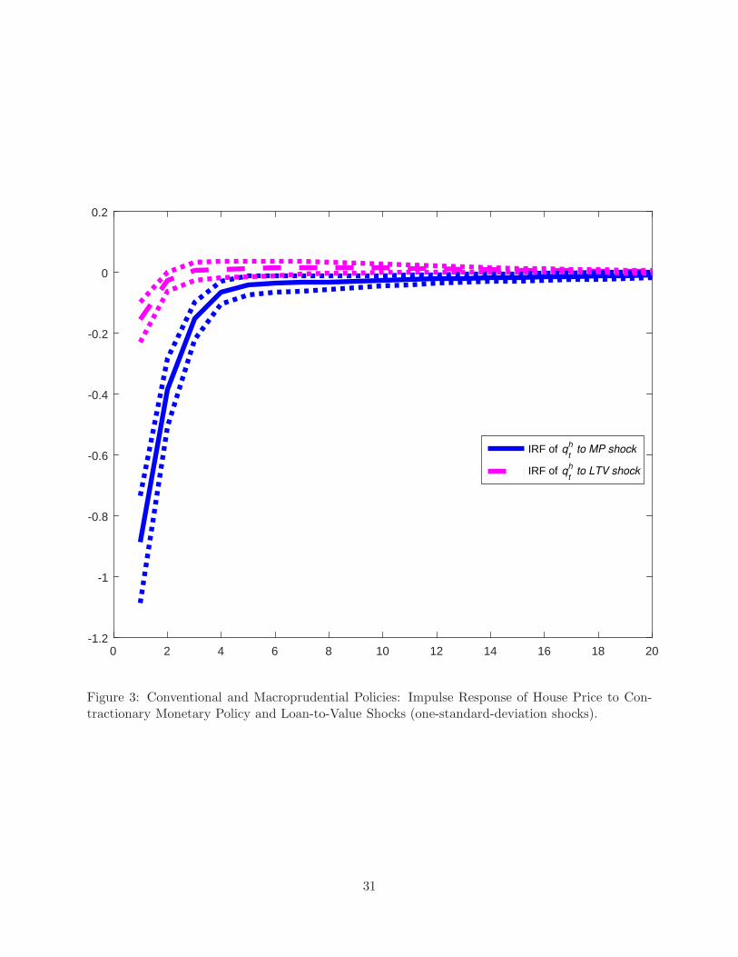
and monetary policy shocks on house prices in Figure 3. Both policies have statistically significant

effects. The adjustment of house prices is similar, but more limited, in response to LTV policy.11

Figure 4 shows the effects of the second macroprudential policy, consisting of changing the

allowed debt-to-income ratio for borrowers. Policymakers introduced a debt-to-income ceiling for

the first time in August 2005. This policy is captured, somewhat bluntly, by varying the bb/Y

ratio in the model from the original 0.8 to a value of 0.4, which matches the policy implemented in

Korea at its inception in 2005, and in different instances over the sample. The effects on impulse

responses are comparable to those obtained for the loan-to-value policy, although slightly lower

in quantitative terms. Consumption and credit respond less strongly to housing demand shocks

when the lower debt-to-income limit is enforced. The other variables do not respond in significantly

different fashions. Credit shocks become less impactful on all the variables analyzed.

11It also has to be noticed that the LTV disturbance modeled here, while it includes the effects of LTV policies, itis also likely to capture more general conditions in the credit market.

16

6 Rational versus Non-Fully-Rational Expectations

in the Housing Market

So far, we have analyzed the strength of macro-housing interactions while adopting the conventional

assumption of rational expectations. Many observers have argued that expectations, particularly

those related to future house prices, have often displayed behaviors that can hardly be consistent

with the rational expectations hypothesis. In many countries, house-price expectations have been

characterized by irrational exuberance or have been extrapolative in nature. In Korea, there have

been discussions on how over some parts of the sample expectations may have been characterized

by similar over-exuberance, while, in more recent years, house price expectations have been more

sluggish and stagnating, possibly as a result of demographic shifts in the country.

Different assumptions on the formation of expectations may crucially alter how the economy

responds to shocks, the overall importance of housing market spillovers, and the impact of stabi-

lization policies. In this section, therefore, we investigate the effects of deviations from rational

expectations in the formation of house-price expectations.

First, we assume that agents lack perfect knowledge on the law of motion for housing prices.

Under rational expectations, they would know that house prices react to the state variables in the

model and to the structural disturbances. They would have perfect knowledge of the coefficients

in these relationships, and they would observe the contemporaneous values of the disturbances.

We relax here those strong informational assumptions by assuming that economic agents form

expectations from a simple learning model.12 The model allows us to capture the extrapolative

nature of expectations that often exist in the housing market, and to also capture possible periods

of over-exuberance as well as prudence. Agents are assumed to form expectations starting from the

following perceived law of motion, or PLM:

qht = β0,t−1 + βqh,t−1qht−1 + ǫt, (36)

where β0,t−1 denotes agents’ varying perceptions about the intercept, βqh,t−1 denotes changing

beliefs about the persistence of house price, and ǫt is an error term.

Unlike under rational expectations, agents have no way of knowing the coefficients in the rela-

tionship. They exploit past data up to each point in the sample t to learn about those coefficients.13

12A sizable literature studies alternatives to rational expectations in macroeconomic models: Evans and Honkapohja(1999, 2009) survey the adaptive learning approach in macroeconomics, and Milani (2012) reviews alternative waysto model the formation of expectations in DSGE settings.

13We note that this may be an over-simplified perceived law of motion. Agents may use information on interestrates, credit conditions, and so forth, in forming their expectations. This is true, but we aim to show a stark example

17

They learn according to the constant-gain learning algorithm:

βt = βt−1 + gR−1t Xt(q

ht − β ′

t−1Xt)′, (37)

Rt = Rt−1 + g(XtX′

t −Rt−1), (38)

where βt = [β0,t, βqh,t]′, Xt = [1, qht−1]

′, and Rt denotes the precision matrix associated to the

beliefs. The coefficient g represents the constant gain, which governs the speed at which agents

revise their beliefs in light of new information. Agents use (36) and the most recently updated

beliefs (37) to form expectations about future house prices Etqht+1.

We estimate the agents’ beliefs and learning process over the sample.14 The inferred evolution

of beliefs regarding house prices is shown in Figure 5. Agents are learning about the intercept, or

steady-state, in the house-price equation, and about the autoregressive coefficient. The perceived

intercept fluctuates over the sample. The perceived persistence parameter remains high over the

full sample. Interestingly, the belief jumps slightly above 1 in the periods right before the Korean

crisis. The belief stabilizes later on and fluctuates gently around values just below 0.9.

We can now compare the importance of housing and credit shocks in the DSGE model under

different assumptions about the formation of expectations: the original rational expectations envi-

ronment, and an alternative in which agents are possibly learning about house prices and forming

non-fully-rational expectations. For the latter option, we consider two cases. One mirrors the

expectation that house prices are close to random walks, which existed in the late 1990s; we show

impulse responses for the case in which βqh,t lies at 0.99. The second captures the more common

stance over the sample that sees beliefs about the autoregressive coefficient fall just below 0.9:

we set βqh,t = 0.875, the average value of beliefs around the sample. The model and parameters

remain the same as in the rational expectations specification, but with the rational expectation

Etqht+1 replaced by the non-fully-rational Etq

ht+1.

15

As evidenced by the forecast error variance decomposition results in Table 3, spillovers from

the housing market to the macroeconomy are substantially larger under non-rational housing ex-

pectations. Housing and credit market shocks explain between 10% and 20% of GDP fluctuations,

depending on the state of beliefs, in contrast to less than 3% when house-price expectations are

in which expectations deviate from rational and that can capture in a way that is as intuitive as possible the effectsof non-rationalities.

14We set the constant gain coefficient equal to 0.1. This value is larger than values often estimated in DSGE models(e.g., Milani (2007, 2011, 2017)), but we feel that a higher gain is motivated by the simplicity of the PLM in question.We have experimented with lower values: the main difference is that housing beliefs become much more stable in thesecond part of the sample.

15Only one-period-ahead expectations matter in our framework. An alternative is to model subjective expectationsthrough the infinite-horizon learning approach, discussed in Preston (2005).

18

modeled as rational. Interestingly, the larger spillovers from the housing market may be more

consistent with the empirical SVAR evidence for Korea: Hwang (2012) finds that housing shocks

explain 16% of the output variance (and up to 30% of the variance if housing and lending shocks

are considered jointly) in a SVAR identified through sign restrictions.

To understand the potential channels for the amplification of housing shocks, we show a selection

of relevant impulse responses in Figure 6. Under extrapolative expectations, agents in the economy

do not recognize all the general equilibrium effects that link house prices to other domestic and

open-economy variables and disturbances. They simply extrapolate from past house prices to form

expectations about the future. House prices do not jump immediately, as they do under rational

expectations, but they display a more protracted adjustment to housing and credit shocks. As a

result, residential investment increases with a delay, but with a larger cumulative effect. Aggregate

consumption falls on impact in response to positive housing preference shocks, but the overall

impact is more modest than under rational expectations. Investment responds positively, with a

persistent effect that lasts for several quarters, before falling below steady state. Fluctuations of

GDP in response to housing demand shocks mirror those in investment, and are larger and more

persistent than they would be under rational expectations.

Under extrapolative expectations, house prices do not decline as much in response to positive

technology shocks in the construction sector. The resulting boom in residential investment is,

therefore, more pronounced, especially with very persistent beliefs.

6.1 Extrapolative Expectations Everywhere

So far, we have assumed that non-rational expectations affect only the formation of house price

forecasts. As a robustness check, we now assume that extrapolative expectations exist for every

variable that also enter in expectation in the model, not just for house prices. For each variable, we

estimate a PLM of the same form as (36), with corresponding coefficients updated as in (37)-(38).

We then consider the average value of beliefs over the sample for each variable and recompute

the share of business cycle fluctuations that can be attributed to the set of housing and credit

shocks. The results, reported in Table 3, are in line with those found before: housing and credit

shocks still explain 24.5% of output fluctuations when extrapolative expectations are pervasive in

the economy.

19

7 Conclusions

In this paper, we studied Korea as an example of a small open economy, which may have been

subject in recent decades to macroeconomic fluctuations that originated in the country’s real estate

market. House prices boomed for decades before falling in the late 1990s, and becoming quite

sluggish by the end of the sample. Household credit has constantly risen, reaching levels that many

believe to be worrying for the stability of the economy. Korea is also an important laboratory, since

policymakers have resorted to macroprudential measures, in addition to conventional monetary

and fiscal policies, to either cool or stimulate the housing market. At different intervals, they have

imposed policies to limit the allowed loan-to-value and debt-to-income ratios for borrowers.

This paper used a structural small open economy model to study the interactions between the

housing market and broader macroeconomy. We estimated the model to fit a large set of domestic

and global macroeconomic variables, along with housing and credit variables. The empirical results

showed that house prices are mainly driven by sector-specific shocks, related to housing demand,

supply, or credit. Housing and credit shocks spill over on the rest of the economy, but, at least under

rational expectations, their overall contribution to aggregate consumption and GDP fluctuations

are modest, falling at 10 and 3% of their variance, respectively.

Macroeconomic dynamics in Korea is largely influenced, instead, by disturbances that are open-

economy in nature: exchange-rate, import-price, terms of trade, and foreign shocks. Those explain

the vast majority of fluctuations in domestic aggregates and also play a role on domestic credit and

construction investment as well.

We analyzed the significance of macroprudential policies through the lens of the microfounded

model. We found both loan-to-value and debt-to-income limits to be effective and well targeted

at reducing volatility caused by housing and credit shocks, without causing broader recessionary

effects.

We emphasized how assumptions about the way in which expectations are formed may affect

both the response of macroeconomic variables to housing and credit shocks and the magnitude

of housing spillovers on the macroeconomy. We replaced rational house-price expectations with

expectations obtained from a constant-gain learning model. The inferred beliefs are characterized

by potentially destabilizing behavior in some parts of the sample and by pronounced sluggishness

over the past fifteen years. The role of housing shocks is magnified when expectations are not

fully rational, in particular in periods in which economic agents believe house prices to be close

to random walks. Under non-rational expectations and learning, the sensitivity of macroeconomic

20

variables to those shocks is increased, and the shocks’ contribution to business cycles becomes much

more significant.

References

Aoki, K., Proudman, J., and Vlieghe, G. (2004), “House Prices, Consumption, and Monetary

Policy: A Financial Accelerator Approach,” Journal of Financial Intermediation, 13, 414–435.

Christensen, I., Corrigan, P., Mendicino, C., and Nishiyama, S.-I. (2016), “Consumption, Housing

Collateral and the Canadian Business Cycle,” Canadian Journal of Economics, 49, 207–236.

Christiano, L. and Fitzgerald, T. J. (2003), “The Band Pass Filter,” International Economic Re-

view, 44, 435–465.

Christiano, L., Eichenbaum, M., and Evans, C. (2005), “Nominal Rigidities and the Dynamic

Effects of a Shock to Monetary Policy,” Journal of Political Economy, 113, 1–45.

Evans, G. W. and Honkapohja, S. (1999), “Learning Dynamics,” Handbook of Macroeconomics, I

A, 449–542.

Evans, G. W. and Honkapohja, S. (2009), “Learning and Macroeconomics,” Annual Review of

Economics, 1, 421–449.

Finocchiaro, D. and Von Heideken, V. Q. (2013), “Do Central Banks React to House Prices?”

Journal of Money, Credit and Banking, 45, 1659–1683.

Fukac, M. and Pagan, A. (2010), “Limited information estimation and evaluation of DSGE models,”

Journal of Applied Econometrics, 25, 55–70.

Funke, M. and Patz, M. (2013), “Housing Prices and the Business Cycle: An Empirical Application

to Hong Kong,” Journal of Housing Economics, 22, 62–76.

Galı, J. and Monacelli, T. (2005), “Monetary policy and exchange rate volatility in a small open

economy,” Review of Economic Studies, 72, 707–734.

Greenwood, J., Hercowitz, Z., and Krusell, P. (1997), “Long-Run Implications of Investment-

Specific Technological Change,” American Economic Review, 87, 342–362.

21

Hahm, J.-H., Mishkin, F. S., Shin, H. S., and Shin, K. (2011), “Macroprudential policies in open

emerging economies,” Proceedings. San Francisco: Federal Reserve Bank of San Francisco, pp.

63–114.

Hwang, Y. (2012), “Sources of Housing Price Fluctuations: An Analysis Using Sign-restricted

VAR,” Korea and the World Economy, 13, 249–283.

Iacoviello, M. (2005), “House Prices, borrowing constraints and monetary policy in the business

cycles,” American Economic Review, 3, 739–764.

Iacoviello, M. and Neri, S. (2010), “Housing Market Spillovers: Evidence from an Estimated DSGE

Model,” American Economic Journal: Macroeconomics, 2, 125–164.

Igan, D. and Kang, H. (2011), “Do Loan-to-Value and Debt-to-Income Limits Work? Evidence

from Korea,” IMF Working Paper 297.

Justiniano, A. and Preston, B. (2010), “Can structural small open-economy models account for the

influnece of foreign disturbances?” Journal of International Economics, 81, 61–74.

Kam, T., Lees, K., and Liu, P. (2009), “Uncovering the Hit List for Small Inflation Targeters: A

Bayesian Structural Analysis,” Journalof Money, Credit and Banking, 41, 583–618.

Kim, K.-H. (2004), “Housing and the Korean Economy,” Journal of Housing Economics, 13, 321–

341.

Lee, J. and Song, J. (2015), “Housing and business cycles in Korea: A multi-sector Bayesian DSGE

approach,” Economic Modelling, 45, 99–108.

Milani, F. (2007), “Expectations, Learning and Macroeconomic Persistence,” Journal of Monetary

Economics, 54, 2065–2082.

Milani, F. (2011), “Expectation Shocks and Learning as Drivers of the Business Cycle,” Economic

Journal, 121, 379–401.

Milani, F. (2012), “The Modeling of Expectations in Empirical DSGE Models: a Survey,” Advances

in Econometrics, 28, 3–38.

Milani, F. (2017), “Sentiment and the U.S. Business Cycle,” Journal of Economic Dynamics and

Control, 82, 289–311.

22

Milani, F. and Park, S. H. (2015), “The effects of globalization on macroeconomic dynamics in a

trade-dependent economy: The case of Korea,” Economic Modelling, 48, 292–305.

Monacelli, T. (2005), “Monetary Policy in a Low Pass-Through Environment,” Journal of Money,

Credit, and Banking, 37, 1047–1066.

Ng, E. C. and Feng, N. (2016), “Housing market dynamics in a small open economy: Do external

and news shocks matter?” Journal of International Money and Finance, 63, 64–88.

Preston, B. (2005), “Learning about Monetary Policy Rules when Long-Horizon Expectations Mat-

ter,” International Journal of Central Banking, 1, 81–126.

Robinson, T. and Robson, M. (2012), “Housing and Financial Frictions in a Small Open Economy,”

mimeo, Reserve Bank of Australia.

Schmitt-Grohe, S. and Uribe, M. (2003), “Closing Small Open Economy Models,” Journal of In-

ternational Economics, 61, 163–185.

Smets, F. and Wouters, R. (2007), “Shocks and Frictions in US Business Cycles: A Bayesian DSGE

Approach,” American Economic Review, 97, 586–606.

A Data Description

We use the following data series as observables in the estimation:

1. Real GDP (detrending: Bandpass filter, Christiano-Fitzgerald)

2. Real Consumption (detrending: Bandpass filter, Christiano-Fitzgerald)

3. Real Non-Residential Investment (detrending: Business Investment) (Bandpass filter, Christiano-

Fitzgerald). The series is computed from Gross Fixed Capital Formation, subtracting resi-

dential investment.

4. Real Residential Investment (detrending: Bandpass filter, Christiano-Fitzgerald)

5. CPI Inflation (log difference, no trend). We use the series for core CPI inflation, excluding

agriculture and energy.

6. Domestic Inflation (GDP Implicit Price Deflator, log difference, no trend)

23

7. Nominal Exchange Rate. We use the inverse of the nominal effective exchange rate published

by the BIS (an increase denotes a depreciation according to the definition in the model). We

take the logarithm of the series and consider in deviation from the sample mean. We allow

for a break in the sample mean in 1998.

8. Nominal Interest Rate. The annual rate is transformed into quarterly rate. The interest rate

is considered in deviation from the sample mean. Again we allow for a break in the mean

before and after 1998.

9. Real House Price Index (detrending: Bandpass filter, Christiano-Fitzgerald)

10. Real Household Credit (detrending: Bandpass filter, Christiano-Fitzgerald). The original

household credit series is seasonally adjusted and deflated using the GDP Implicit Price

Deflator.

11. Terms of Trade (Net barter definition, we detrend using a linear trend).

12. Foreign Output (weighted average of Christiano-Fitzgerald detrended GDPs for the top 10

trading partners: USA, Japan, China, Germany, France, Netherlands, Switzerland, U.K.,

Singapore, and Hong Kong). The time-varying weights are computed as the sum of exports

plus imports with the specific partner, as a fraction of their total sum.

13. Foreign Inflation (log difference, no trend, weighted average computed as before)

14. Foreign Interest Rate (re-expressed in quarterly rate, weighted average computed as before)

The series are at quarterly frequency and spanning the sample between 1991:I and 2014:IV. The

series have been obtained from the Bank of Korea.

B Full List of Model Equations

We present here the full list of log-linearized model equations. The subscript j = s, b indicates

savers or borrowers. Subscripts c and h for labor variables refer to labor in the consumption or

housing sector, respectively.

ct =ωcs,t + (1− ω)cb,t

ht =ωhs,t + (1− ω)hb,t

nj,t =Nj,c

Njnj,c,t +

Nj,h

Njnj,h,t

24

cs,t =η

1 + ηcs,t−1 +

1

1 + ηEtcs,t+1 −

(1− η)

1 + η(Rt − Etπt+1 +∆ζt+1)

cb,t =βsη

βs + βbηcb,t−1 +

1

βs + βbηEtcb,t+1 −

βs(1− η)

βs + βbη(Rt − Etπt+1)+

+βs(1− η)

βs + βbη(1− ρζ

βbβs

)ζt +βs(1− η)(βs − βb)

βsβb(βs + βbη)(Λt +Rt)

wj,t =ψnj,t +1

1− η(cj,t − ηcj,t−1)− ζt

it =1

1 + βsit−1 +

βs1 + βs

Etit+1 +1

(1 + βs)ϕ(qt + µt)

qt =βs(1− δ)Etqt+1 + βsrkEtr

kt+1 − (Rt − EtπH,t+1)

kt =(1− δ)kt−1 + δ(µt + it)

iht =1

1 + βsiht−1 +

βs1 + βs

Etiht+1 +

1

(1 + βs)ϕhqkht

qkht =(1− βs(1− δkh))(rht+1 − τht + Etπt+1

)+ βs(1− δkh)Et(q

kht+1 + πH,t+1)−Rt

kht =(1− δkh)kht−1 + δkhiht

hs,t =βs(1− δh)

1− βs(1− δh)Et

[ζt+1 −

1

1− η(cs,t+1 − ηcs,t) + qht+1 − qht

]+

−1

1− βs(1− δh)

[ζt −

1

1− η(cs,t − ηcs,t−1)

]+ jt

hb,t =βb(1− δh)

(1− βb(1− δh) + m(βs − βb))Et

[1

1− η(cb,t+1 − ηcb,t)− ζt+1 + qht+1

]

−1

(1− βb(1− δh) + m(βs − βb))

[1

1− η(cb,t − ηcb,t−1)− ζt

]

−m(βs − βb)

(1− βb(1− δh) + m(βs − βb))

(Λt +mt + Et

[πt+1 + qht+1

])− qht + jt

bb,t =m(mt + hb,t + Et

[qht+1 + πt+1

]−Rt

)

hj,t =δhihj,t + (1− δh)hj,t−1

ht =δhiht + (1− δh)ht−1

bbYbb,t =

CbYcb,t +

qhHb

Y

(δhqht + hb,t − (1− δh)hb,t−1

)+

1

βs

bbY(Rt−1 + bb,t−1 − πt)+

−WbNb,c

Y(wb,t + nb,c,t)−

WbNb,h

Y(wb,t + nb,h,t)−

rl

Yrlt

nj,c,t =mct + yt − γτt − wj,t

nj,h,t =qht + iht − wj,t

rkt =mct + yt − kt−1

rht =qht + iht − kht−1

rlt =qht + iht

25

iht =at + aht + ǫhkht−1 + ǫllt + (1− ǫh − ǫl)(νns,h,t + (1− ν)nb,h,t)

πt =(1− γ)πH,t + γπF,t

πH,t =β

1 + βγHEtπH,t+1 +

γH1 + βγH

πH,t−1 +(1− βθp)(1− θp)

(1 + βγH)θpmct + εpt

mct =ǫ(1− α)ws,t + (1− ǫ)(1− α)wb,t + αrkt − at + (1− α)γτt

πF,t =β

1 + βγFEtπF,t+1 +

γF1 + βγF

πF,t−1 +(1− βθF )(1 − θF )

(1 + βγF )θF[rert − (1− γ)τt] + εipt

∆rert =∆et − (πt − π∗t )

Et∆et+1 =Rt −R∗

t + χnfat + εφt

nfat =β−1s

(nfat−1 +∆yt +∆et +R∗

t−1 − πH,t + εφt

)+

(1¯nfa

)X

Y(xt − yt)

−

(1¯nfa

)Cm

τhY(ct + rert − (σ(1 − γ)− γ)τt)

∆τt =πF,t − πH,t + ετt

∆τht =πH,t − πt

xt =σ∗(rert + γτt) + y∗t

GDPt =Y τh

¯GDP(yt + τht ) +

qh ¯IH¯GDP

(qht + iht)

yt =Ch

Y(ct + γστt) +

I

Yit +

Ih

Yiht +

X

Yxt + εgt

Rt =ρRt−1 + (1− ρ)[ψππt + ψGDP∆GDPt + ψqh∆q

ht + ψe,t∆et

]+ εmpt

26

Description Parameters Prior Distributions Posterior Mean 95% PPI

Share of patient households ω B(0.65, 0.05) 0.68 [0.61,0.75]Habit formation η B(0.5, 0.2) 0.67 [0.62, 0.72]Adj. cost i ϕ Γ(4, 1.5) 4.49 [3.19,6.14]Adj. cost iH ϕkh Γ(4, 1.5) 5.39 [3.96,7.14]Indexation (Dom.) γH B(0.7, 0.1) 0.48 [0.29, 0.70]Calvo (Dom.) θH B(0.75, 0.1) 0.63 [0.52, 0.72]Indexation (Imports) γF B(0.7, 0.1) 0.44 [0.27, 0.65]Calvo (Imports) θF B(0.75, 0.1) 0.85 [0.79, 0.89]MP inertia ρ B(0.7, 0.1) 0.65 [0.58, 0.71]MP reaction to infl. ψπ N(1.5, 0.125) 1.54 [1.34, 1.75]MP reaction to output ψy Γ(0.125, 0.0625) 0.08 [0.04, 0.12]MP reaction to ER ψ∆e Γ(0.15, 0.15) 0.01 [0.00, 0.03]MP reaction to house price ψ∆qh Γ(0.05, 0.05) 0.19 [0.06, 0.34]

AR Preference ρζ B(0.5, 0.2) 0.45 [0.36, 0.52]AR Inv. Spec. ρµ B(0.5, 0.2) 0.61 [0.45, 0.74]AR Housing Demand ρj B(0.5, 0.2) 0.90 [0.85, 0.94]AR credit ρm B(0.5, 0.2) 0.91 [0.84, 0.96]AR technology ρa B(0.5, 0.2) 0.80 [0.68, 0.89]AR tech. housing ρah B(0.5, 0.2) 0.99 [0.97, 0.998]AR cost-push imports ρip B(0.5, 0.2) 0.15 [0.08, 0.24]AR risk premium ρφ B(0.5, 0.2) 0.82 [0.75, 0.87]AR govt spending ρg B(0.5, 0.2) 0.92 [0.87, 0.97]AR foreign output ρy∗ B(0.2, 0.05) 0.20 [0.11, 0.31]AR foreign infl. ρπ∗ B(0.2, 0.05) 0.20 [0.11, 0.31]AR foreign int. rate ρi∗ B(0.2, 0.05) 0.20 [0.11, 0.30]Std. Preference σζ Γ−1(5,∞) 0.70 [0.57, 0.86]Std. Inv. Spec. σµ Γ−1(5,∞) 4.10 [3.09, 5.45]Std. Housing Demand σj Γ−1(5,∞) 0.88 [0.67, 1.14]Std. credit σm Γ−1(5,∞) 3.20 [2.58, 3.94]Std. technology σa Γ−1(5,∞) 0.95 [0.75, 1.20]Std. tech. housing σah Γ−1(5,∞) 1.90 [1.54, 2.37]Std. cost-push σp Γ−1(1,∞) 1.41 [1.13, 1.77]Std. cost-push imports σip Γ−1(1,∞) 1.35 [1.14, 1.60]Std. risk premium σφ Γ−1(5,∞) 1.30 [0.94, 1.77]Std. MP σmp Γ−1(1,∞) 0.45 [0.38, 0.53]Std. govt spending σg Γ−1(1,∞) 1.48 [1.29, 1.72]Std. tot στ Γ−1(1,∞) 4.09 [3.54, 4.78]Std. foreign output σy∗ Γ−1(1,∞) 0.59 [0.51, 0.68]Std. foreign infl. σπ∗ Γ−1(1,∞) 0.34 [0.30, 0.40]Std. foreign int. rate σi∗ Γ−1(1,∞) 0.11 [0.10, 0.13]

VAR Coeffs f11 B(0.8, 0.1) 0.90 [0.83, 0.96]” f12 N(0, 0.125) 0.07 [-0.13, 0.27]” −f13 Γ(0.25, 0.15) 0.14 [0.03, 0.36]” f21 Γ(0.1, 0.05) 0.05 [0.02, 0.08]” f22 B(0.8, 0.1) 0.70 [0.54, 0.86]” −f23 Γ(0.1, 0.05) 0.07 [0.02, 0.15]” f31 Γ(0.1, 0.05) 0.01 [0.00, 0.02]” f32 Γ(0.1, 0.05) 0.04 [0.02, 0.08]” f33 B(0.8, 0.1) 0.85 [0.79, 0.90]

Table 1: Prior Distributions and Posterior Estimates.Note: Γ denotes Gamma distribution, B Beta distribution, N Normal distribution, and Γ−1 Inverse Gamma distri-

bution. The prior distributions are expressed in terms of mean and standard deviation.

27

Short Run: horizon = 4 Business Cycle: horizon = 32

Domestic Shocks Housing & Credit Shocks Open-Economy Shocks Domestic Shocks Housing & Credit Shocks Open-Economy Shocks

gdpt 52 1 47 12 3 85

ct 78 2 20 25 5 70

it 61 6 33 22 10 68

iht 26 55 19 11 54 35

qht 13 70 17 4 88 8

bb,t 25 67 8 22 36 42

πt 42 9 49 22 6 72

et 5 2 93 4 5 91

Rt 30 21 49 12 10 78

Table 2 - Forecast Error Variance Decomposition (Model with Rational Expectations). Note:

Percentage of variance explained by each group of shocks: domestic (preference, investment-specific, technology, price

markup, monetary policy, and government spending), housing and credit (housing preference, housing technology,

and loan-to-value), and open-economy (foreign output, foreign inflation, foreign interest rate, risk-premium, terms of

trade, and import-price, shocks).

Rational Expectations AL for Etqht+1 AL everywhere

βqh,t = 0.875 βqh,t = 0.99

gdpt 3% 10.6% 21.4% 20.4%

Table 3 - Forecast Error Variance Decomposition (Model with Rational Expectations). Note:

Percentage of variance explained by housing and credit shocks.

28

1990 2000 2010−10

0

10Real GDP

1990 2000 2010−20

0

20Real Cons

1990 2000 2010−50

0

50Real Bus Invest

1990 2000 2010−20

0

20Real Res Invest

1990 2000 2010−5

0

5CPI Infl

1990 2000 2010−5

0

5Domestic Infl

1990 2000 2010−6

−5

−4Nom Exch Rate

1990 2000 20100

5

10Nom Int Rate

1990 2000 2010−50

0

50Real House Price

1990 2000 2010−50

0

50Real Househ. Credit

1990 2000 2010−5

0

5Foreign Real GDP

1990 2000 2010−2

0

2Foreign Infl

1990 2000 20100

1

2Foreign Interest Rate

1990 2000 2010−20

0

20Terms of Trade

Figure 1: Data Series used as observable variables in the estimation.

29

0 5 10 15-0.5

0

0.5IRF to j

0 5 10 15-0.5

0

0.5IRF to m

0 5 10 15-4

-2

0

0 5 10 15-0.2

0

0.2

0 5 10 15-0.5

0

0.5

0 5 10 15-0.1

0

0.1

0 5 10 150

1

2

0 5 10 15-0.5

0

0.5

0 5 10 150

10

20

0 5 10 150

10

20

0 5 10 150

0.2

0.4

0 5 10 15-0.05

0

0.05

0 5 10 150

0.2

0.4

0 5 10 15-0.05

0

0.05

m=0.4

m=0.6

(it)

(ct)

(qt

h)

(gdpt)

(bb,t

)

(πt)

(Rt)

Figure 2: Macroprudential policy: changes in the Loan-to-Value ratio. Impulse Responses to one-standard-deviation housing preference and ltv shocks.

30

0 2 4 6 8 10 12 14 16 18 20-1.2

-1

-0.8

-0.6

-0.4

-0.2

0

0.2

IRF of qt

h to MP shock

IRF of qt

h to LTV shock

Figure 3: Conventional and Macroprudential Policies: Impulse Response of House Price to Con-tractionary Monetary Policy and Loan-to-Value Shocks (one-standard-deviation shocks).

31

0 5 10 15-0.5

0

0.5IRF to j

0 5 10 15-0.5

0

0.5IRF to m

0 5 10 15-4

-2

0

0 5 10 15-0.2

0

0.2

0 5 10 15-0.5

0

0.5

0 5 10 15-0.2

0

0.2

0 5 10 150

5

10

0 5 10 150

10

20

0 5 10 150

0.2

0.4

0 5 10 15-0.05

0

0.05

B b /Y=0.4

B b /Y=0.8

0 5 10 15-0.1

0

0.1

0 5 10 150

1

2

0 5 10 150

0.2

0.4

0 5 10 15-0.05

0

0.05

(it)

(ct)

(qt

h)

(gdpt)

(bb,t

)

(πt)

(Rt)

Figure 4: Macroprudential policy: changes in the Debt-to-Income limit. Impulse Responses toone-standard-deviation housing preference and ltv shocks.

32

1990 1995 2000 2005 2010 2015−1.5

−1

−0.5

0

0.5

1Adaptive−Learning Beliefs in the formation of House−Price Expectations E

tq

t+1h

Intercept β0,t

1990 1995 2000 2005 2010 20150.7

0.75

0.8

0.85

0.9

0.95

1

1.05

AR coeff β

qh,t

Figure 5: Evolution of House-Price Beliefs, as estimated over the sample.

33

0 5 10 15 20 25 30-10123

IRF of qt

h to j

0 5 10 15 20 25 30-0.2

0

0.2

0.4IRF of q

t

h to m

0 5 10 15 20 25 30

-2

0

2IRF of q

t

h to ah

0 5 10 15 20 25 30-2

0

2

4

IRF of iht to j

0 5 10 15 20 25 300

5IRF of ih

t to a

h

0 5 10 15 20 25 30-0.5

0

0.5IRF of c

t to j

0 5 10 15 20 25 30

-10

-5

0

5IRF of i

t to j

0 5 10 15 20 25 30-1

-0.5

0

0.5IRF of gdp

t to j

Figure 6: Impulse responses under alternative expectation formation assumptions: RE (solid blueline), learning with almost ‘random-walk’ beliefs (βqh,t = 0.99, dashed red line), learning withstable, but persistent, beliefs (βqh,t = 0.875, dash-dot magenta line).

34