1   

Expectation Accuracy, Cost Behavior, and Slippery Prices

ABSTRACT

This study investigates the relation between the accuracy of managerial demand

expectations and cost behavior. Based on a unique dataset of 4,107 firm-year observations from

737 companies in Denmark, this paper first shows that cost stickiness is substantially stronger for

unforeseen negative demand shocks than for expected demand shocks, which is in line with the

argument that adjustment costs are typically higher when the time horizon for making the

adjustments is shorter. Second, we find empirical evidence that omitting selling price changes

can mislead researchers’ inferences about resource adjustments and cost stickiness when sales

are used as a proxy for activity level, which is a common practice in the existing literature.

Finally, we show a moderating effect of managerial expectation accuracy on the relationship

between demand volatility and cost elasticity. This helps reconciling the ongoing debate on

whether companies increase or decrease cost elasticity in response to demand volatility.

Keywords: cost behavior; cost stickiness; resource adjustment costs; managerial decision-

making; slippery prices; demand volatility.

JEL Classifications: D24; M41; P22.

 

2   

INTRODUCTION

Manager’s expectations about future demand are central to the theories of cost behavior,

such as cost stickiness1 (Anderson et al. 2003; Banker et al. 2014; Chen et al. 2013; Chen et al.

2015; Venieris et al. 2015) and cost elasticity (Banker et al. 2014; Holzhacker et al. 2015).

However, prior studies on cost behavior usually do not distinguish between accurate and

inaccurate expectations. Exploiting unique data on managers’ expectations from the Danish

business register,2 we extend this line of research by suggesting that expectation accuracy is

negatively related to cost stickiness.3 We derive this prediction from the fact that adjustment

costs are conditional upon the available time horizon for making the adjustment. Although all

costs are variable in the long run (Horngren et al. 2015, 55; Varian 1992, 65), ad hoc adjustments

can be – sometimes prohibitively – expensive. Accordingly, economic theory suggests that firms

react differently to expected compared to unexpected changes in demand (Hamermesh 1993).

Specifically, firms surprised by a negative demand shock will not be able to adjust their costs

downward as smoothly as companies that accurately expected the shock. Therefore, we argue

that cost stickiness is lower in companies that correctly anticipate future demand. The Danish

data from the joint harmonized EU program of business and consumer surveys, matched with

financial statement information, supports our hypothesis.

                                                        

1 Whereas traditional cost models assume that cost behavior can be approximated by a linear function between total cost and the level of activity (e.g., Horngren et al. 2015; Noreen 1991), the sticky cost literature shows that costs move differently in response to positive compared to negative changes in demand. Specifically, costs are considered sticky if the change in costs is greater for activity increases than for equivalent activity decreases (e.g., Anderson et al. 2003; Anderson et al. 2007; Balakrishnan et al. 2004; Balakrishnan and Gruca 2008; Chen et al. 2012; Dierynck et al. 2012; Weiss 2010).  2 Prior studies in economics (Bennedsen et al. 2007; Amore and Bennedsen 2013) and management (Dahl and Sorenson 2012; Dahl et al. 2012) used data from the Danish business register. 3 Expectation accuracy captures the degree to which managers’ beliefs about future demand coincide with the actual path of demand.

3   

We continue by investigating the potentially confounding effect of price changes for cost

stickiness estimations (Cannon 2014). Omitting selling price changes can lead to incorrect

conclusions (i.e., concluding that costs are sticky when in fact only prices change). Yet few

studies have included prices, most likely due to data availability constraints. Our analyses

suggest that price changes can indeed alter the conclusions derived from the standard cost

stickiness model.

Finally, we exploit our unique measure of expectation accuracy to revisit the debate in

the literature whether companies increase or decrease cost elasticity in response to demand

volatility.4 Whereas Holzhacker et al. (2015) provide evidence for the traditional view that

companies with higher demand volatility prefer more variable cost structures to reduce

downward risk, Banker et al. (2014) find that congestion cost can lead to the opposite effect (i.e.,

companies with higher demand volatility prefer more rigid cost structures). We replicate their

approach and find support for Banker et al.’s (2014) results. Then we investigate the effect of

demand volatility conditional upon expectation accuracy. We find that the association between

demand volatility and cost elasticity reverses (i.e., becomes consistent with Holzhacker et al.

(2015)) for observations where demand decreases and expectation accuracy is high. This result

provides a potential key to reconcile both prior studies. Not only can prior studies’ findings be

replicated, but – as will be described later – the conditions under which the effects switch

direction also seem empirically descriptive of the research settings of Banker et al. (2014) and

Holzhacker et al. (2015).

                                                        

4 Prior literature often uses the term “demand uncertainty” and measures this variable as the firm-level time-series standard deviation of output (Holzhacker et al. 2015, 2316; Banker et al. 2014, 849). We prefer the label “demand volatility” for this empirical proxy because even among firms with the same “demand volatility” for some firms the demand will be more predictable (i.e., less uncertain) than for others.

4   

Overall, this paper contributes to cost behavior research in three ways. First, our findings

show that the firm’s degree of cost stickiness is contingent upon expectation accuracy. Second,

we provide evidence that omitting price changes can alter the conclusions derived from the

traditional cost stickiness estimation approach. Third, this study helps reconcile inconsistent

findings in the prior literature regarding the association between demand volatility and cost

elasticity.

THEORY AND HYPOTHESIS DEVELOPMENT

Accuracy of Managerial Expectations and Asymmetric Cost Behavior

Managers’ expectations about future demand drive asymmetric cost behavior. Research

suggests that, if the adjustment of resources is costly, an executive who is optimistic with respect

to future demand is more willing to build up or retain resources than a manager who expects a

prospective decrease in demand. Thus, positive expectations are associated with a higher degree

of cost stickiness. To test this relationship, several measures are used as proxies for management

expectations. These include variables such as GDP growth (Anderson et al. 2003; Banker et al.

2014), order backlog (Balakrishnan et al. 2004; Banker et al. 2014), the tone of forward-looking

statements in 10-K reports (Chen et al. 2015), analyst forecasts (Banker et al. 2014), intangible

investments (Venieris et al. 2015),5 and managerial overconfidence (Chen et al. 2013).6

However, none of these studies have distinguished between expected and unexpected

changes in demand by investigating whether the anticipated path of future sales is realized.

However, doing so can alter previous inferences. For instance, higher cost rigidity (i.e., lower

                                                        

5 Venieris et al. (2015) argue that high levels of intangible assets reflect investments in organizational capital that is required to support the company’s long-term growth strategy. Hence, high intangible assets are associated with optimistic sales expectations. 6 According to Chen et al. (2013), overconfident managers are more likely to a) overestimate their impact of restoring demand when sales decline and b) overestimate the accuracy of their assessment of prospective demand. Therefore, overconfident managers are more optimistic with respect to future sales.

5   

cost elasticity) can result from a delayed adjustment of capacity. Examples of such unexpected

shocks can include customer credit failure, the launch of competitive products, and currency

fluctuations. Moreover, it is often difficult to quickly downsize costs when unexpected demand

decreases occur, such as due to employee protection laws or company reputation considerations

(Banker et al. 2013a; Bentolila and Bertola 1990).

As Figure 1 indicates, adjusting resources to shocks in demand is contingent upon the

accuracy of expectations. If the firm correctly anticipates an economic downturn, it can initiate

the necessary steps for resource adjustment before the shock hits; thus, cost reductions can begin

more quickly once the shock occurs. Yet if the shock is completely unexpected, the firm cannot

pre-adjust to the actual path of demand. Rather, the decision-maker realizes the shock only after

it occurred initially (Hamermesh 1993). This leads to a delayed and more abrupt adjustment of

resources relative to the actual level of demand.

Economic theory typically assumes that adjustment costs follow a quadratic function

(Hamermesh 1993, 210). “This means that it is very costly for the firm to move instantaneously

between static equilibria, because compressing the change in employment into a very small

period of time causes costs to rise with the square of the change” (Hamermesh 1993, 210).

Lower expectation accuracy makes it more difficult to smooth resource adjustments. Thus,

changes may occur more abruptly, which will lead to higher adjustment costs for companies that

face a convex adjustment cost function (Hamermesh and Pfann 1996). For example, redundancy

payments will usually be higher for large abrupt layoffs compared to small and gradual

workforce adjustments.

[Insert Figure 1 about here]

6   

In a positive demand shock, companies generally try to increase their output. However,

companies that do not expect the demand increase are more likely to have higher adjustment

costs, if they adjust in a shorter time span. For example, hiring more workers in a short period of

time will probably lead to marginally increasing costs, if the company has to use additional

search channels or recruit workers further away etc. Similarly, finding a bigger facility to rent

will be more costly, if the deal has to be closed under time pressure. Additionally, an unexpected

increase in customer orders may lead to higher selling related costs due to process disruptions,

for example if the distributing warehouse runs out of capacity or if the usual distributors reach

their maximum capacity and alternative delivery services have to be found.

Related to the previous examples, firms that did not expect a rise in demand are more

likely to respond to a positive demand shock by using overtime work or short-term labor, which

often requires the payment of a premium. In comparison, marginal costs rise less in companies

that correctly anticipate positive demand shock. These companies can increase capacity in a

more timely manner, thereby reducing congestion costs and mitigating organizational

disruptions.

Taken together, the arguments about adjustments after positive and negative demand

shocks explained above suggest that the downward slope is steeper and the upward slope is less

steep for companies with higher managerial expectation accuracy (see Figure 2). Accordingly,

the cost stickiness coefficient in empirical estimations would be lower for managers with higher

expectation accuracy.

H1: The degree of cost stickiness decreases with increasing accuracy of managers’ demand

anticipations.

7   

Managerial Expectations and Price Adjustments

Firms do not react to expected changes in demand solely by cutting or adding resources;

they can also adjust selling prices. Prior literature suggests that adjustments are costly for both

capacity (Hamermesh and Pfann 1996; Hayashi 1982) and prices (Mankiw 1985; Rotemberg

1982). To keep adjustment costs low, decision makers choose the least expensive mechanism in

response to demand changes. Under uncertainty, the optimal capacity and pricing decision

depends on what is known about demand at the time of the decision and the incorporation of new

information over the planning cycle (Goex 2002).

Following Anderson et al. (2003), many studies estimate the elasticity of cost response to

variations in demand by regressing the change in costs on the change in sales. The statistical

specification is as follows:

∆ln , β , ∙ ∆lnSALES , , , where , ∙ , (1)

∆ln , and ∆lnSALES , capture the natural log-change between the current and the previous

period in costs and sales, respectively, and , is an indicator variable set to one when sales

decrease and zero otherwise. In the standard model, according to Anderson et al. (2003), the

implied association is estimated using SG&A costs. SG&A costs are sticky on average if 0

and 0. The general intuition is that managers retain idle capacity during periods of

declining demand to avoid adjustment costs (Anderson et al. 2003; Banker and Byzalov 2014).

However, using sales as a proxy for activity, empiricists may also observe a significant

cost stickiness coefficient irrespective of changes in labor or capital resources. Specifically, costs

appear to be sticky if managers adjust selling prices asymmetrically – that is, they lower prices to

exploit existing capacity when demand decreases but build up capacity (instead of raising prices)

when demand increases (Cannon 2014). Thus, the investigation of cost behavior based on a

8   

model that uses sales instead of actual activity is more precise when selling price changes can be

controlled for. We will return to this point in the results section.

Accuracy of Managerial Expectations and Cost Elasticity

Based on the arguments above the empirically observed cost functions are contingent

upon expectation accuracy. Therefore we suggest that managerial expectation accuracy is also

relevant for the recent work which analyzes the interplay between demand volatility and

managers’ resource adjustment decisions. Banker et al. (2014) argue that firms will try to avoid

congestion by choosing a more rigid cost structure (i.e., more fixed and less variable costs) when

demand volatility is high. This argument challenges conventional thinking by claiming that the

value of flexibility decreases with uncertainty. Using a combined analytical and empirical

approach, Banker et al. (2014) show that marginal costs increase with increasing congestion due

to the convexity of the cost function. Therefore, to prevent expensive bottlenecks, managers

invest in fixed capacity when demand is uncertain and the likelihood of extreme realizations of

demand is higher.

Holzhacker et al. (2015) explore actions through which managers alter the company’s

cost structure in response to demand volatility and financial risk. Their results show that

decision-makers deliberately adapt cost elasticity through three main mechanisms: leasing

instead of purchasing equipment, engaging in flexible work contracts, and outsourcing.

Interestingly, Holzhacker et al. (2015) find opposite results to Banker et al. (2014) – that is,

demand volatility is positively associated with cost elasticity. In our additional analysis we

demonstrate how expectation accuracy can help to reconcile these conflicting findings. We show

in the appendix how Banker et al.’s (2014) analytical model can be extended to incorporate the

empirical findings of our study.

9   

RESEARCH DESIGN AND SAMPLE SELECTION

Data and Sample Selection

We analyze 4,107 firm-year observations from 737 Danish companies from 1999 to 2013

using micro-data from a business and consumer survey conducted by Denmark Statistics that we

matched to financial statement information.7 This unique dataset provides several advantages.

Most importantly, the data contain information on managers’ expectations about future demand

and actual demand development, thereby allowing for the construction of an empirical measure

of expectation accuracy. In addition, the business and consumer survey also provides information

on selling price changes that circumvents some empirical design weaknesses in prior studies

(Anderson and Lanen 2009; Cannon 2014).8 The survey was launched as part of a harmonized

EU-wide study with the objective of gaining insights into economic trends, short-term

developments, and potential turning points in the economic cycle (European Commission 2014).

Authorized Danish research institutions are eligible to submit a project proposal that allows

approved scholars to purchase access rights to firm-specific data. The interplay between the

accuracy of managerial expectations, resource adjustment decisions, and price changes can thus

be studied on a firm basis instead of using aggregate information.

Following the grouping of the original survey, the allocation of observations in the

manufacturing, service, construction, and trade sectors is 48 percent, 41 percent, 9 percent, and 2

percent, respectively. Because the manufacturing sector is the largest and greatest contributor to

the GDP in Denmark, it serves as the reference group for the following regressions.

                                                        

7 https://www.dst.dk/en/Statistik/emner/erhvervslivet-paa-tvaers/konjunkturbarometre 8 Another advantage of the dataset is that potential biases of empirical estimates due to information asymmetry or goal incongruence are mitigated because almost all companies in the sample are privately owned (Chen et al. 2012).

10   

Raw data obtained from Denmark statistics are provided in separate files for each month

and sector. The monthly datasets were first cleansed9 and aggregated by year to allow the match

with the annual financial statements. The financial statement information of private and public

listed firms on sales,10 operating income, depreciation, total assets, and personnel expenses was

obtained from the Orbis database maintained by Bureau Van Dijk. To ensure anonymity,

Denmark Statistics (not the researchers) matched the financial statement data with the EU panel

survey data. We conducted each analysis on Denmark Statistics’ secure server.

Because SG&A costs are not stated as separate line items, the amount is indirectly

calculated by subtracting operating income, depreciation, and costs of goods sold (for non-

service firms) from operating sales per company. All financial variables are deflated to year 2000

DKK values.

In line with Anderson et al. (2003), observations with missing data on SG&A costs, sales,

and observations with greater SG&A costs than sales are deleted. To reduce the influence of

outliers, the sample is trimmed at 1 percent and 99 percent of the distribution. Moreover,

monthly data on managers’ assessment of future sales over the next three months and

information on actual sales development of the last three months are necessary.11 We also require

                                                        

9 For example, firm-month observations for which the same company ID occurs in different sectors are allocated to the sector in which the firm was listed with the majority of observations. 10 In Denmark, small and medium size companies only have to report sales; not operating sales. Thus, we use sales instead of operating sales when operating sales it is not available. 11 To reduce the potentially confounding effect of demand volatility, we restrict our sample to observations where the reported demand changed at the beginning and end of the three-month reporting period (i.e., change from report in t to t+1 and from t+3 to t+4). This approach also safeguards that the following empirical estimations are not influenced by the length of the demand shock, as Anderson et al. (2003) suggested. To further alleviate this concern, a supplementary robustness check is conducted in which the degree of cost stickiness for firms with a very low accuracy of managerial expectations and for firms with a moderate accuracy of managerial expectations is compared among companies with the same time frame of the demand shock. Results indicate that potential biases due to differences in the length of the demand shock are not a concern in the subsequent analyses.

11   

firms to have at least five valid observations for the computation of the dependent variable

(natural log-change in SG&A costs).

We tested our hypothesis on two samples. The first sample (i.e., the “whole sample”)

contains all firm-year observations from 1999 to 2013. To ensure that results are not driven by

very pessimistic managerial expectations during the financial crisis (Banker et al. 2013b), the

second sample (i.e., the “reduced sample”) excludes observations from 2007 and 2008.

Model Specification and Variable Measurement

We estimated cost stickiness based on the following regression models. Model (2) refers

to the main model without additional control variables; model (2’) refers to the specification that

contains all control variables.

Without controls:

∆ln & , β , ∙ ∆lnSALES , ∙ , , (2)

where , ∙ ,

With controls:

∆ln & , β , ∙ ∆lnSALES , ∙ , ∙ , , (2’)

where

, ∙ , ∙ , ∙ ,

The change-specification captures the short-term elasticity of SG&A costs in response to a

variation in sales and follows previous studies based on the standard model introduced by

Anderson et al. (2003). is interpreted as the percentage change in SG&A costs per 1 percent

change in sales. The indicator variable , distinguishes the cost response between increases and

12   

decreases in demand. Hence, cost stickiness implies lower cost elasticity for decreases in

demand, which is reflected in a flatter slope of the cost function ( < 0).12

To test our hypothesis, we investigate whether the cost stickiness coefficient is

contingent upon expectation accuracy. In the case of a negative demand shock, the degree of cost

stickiness is predicted to be lower for firms that correctly anticipated it. These firms will start

cutting costs more quickly to avoid a decrease in profitability. Accordingly, our hypothesis is

supported if is larger (i.e., less negative) in the high accuracy subsample than in the low

accuracy subsample.

Similarly, the magnitude of SG&A cost increases is predicted to be lower if a positive

demand shock has been expected. Predicted effects are illustrated in Figure 2.

[Insert Figure 2 about here]

In our main estimation we split the sample by the median and estimate separately for

low expectation accuracy firms vs. high expectation accuracy firms. In the additional analyses,

we also use interactions with a continuous , variable. , is the natural

logarithmic transformation of the percentage of months during which future sales were correctly

anticipated within one year. Because the survey elicited managers’ expectations about demand

over the next three months and actual demand development over the past three months,

                                                        

12 The log-model has several advantages over the linear model. First, the log-transformation alleviates heteroscedasticity and increases the comparability of variables across firms. Second, the logarithmic specification produces a more symmetric distribution than the linear model. Third, the logarithm facilitates an interpretation of the regression coefficients as elasticities (Anderson et al. 2003).

13   

expectations are considered to be correct if the anticipated demand in t is equivalent to the actual

demand in t+3.13 The calculation is:

, % 1

with %#

#

Because the values of % are confined to the interval between 0 and 1 and the natural

log-transformed values range from ∞ to +∞, the application of the logistic measure induces a

more normalized distribution through a reduction of positive skewness.14 An overview of

possible combinations of managerial expectations and actual demand realizations is provided in

Figure 3.

[Insert Figure 3 about here]

Control variables are also incorporated in the slope and intercept of model (2’). Differences in

adjustment costs and size among firms are controlled for by including the empirical proxy of

employee and asset intensity (Anderson et al. 2003; Banker and Byzalov 2014) in the regression

model.15 Employee intensity is measured as the amount of personnel expenses divided by sales

, , and asset intensity is measured as the amount of total assets divided by sales

                                                        

13 See Table A2 in Appendix 1 for a description of survey questions. 14 As a robustness check, we alternatively calculate the %Correct variable as # of months with correct expectations scaled by 12 months instead of scaled by the number of reported months. This approach reduces %Correct. Nevertheless, all results (untabulated) remain substantially similar. 15 Although the majority of studies do not separately control for size when including employee intensity and asset intensity, we conducted a robustness check by testing if parameter estimates differ after including the natural log-amount of total assets in model (2’). Results are largely robust when we also control for size.

14   

, .16 Acknowledging Balakrishnan et al.’s (2014) objections and Balakrishnan et

al.’s (2004) findings, the model controls for industry differences and capacity utilization

, .17 The latter is defined as in Banker et al. (2014), who capture high capacity

utilization with an indicator variable set to one if sales in the previous year increased and zero

otherwise. Because prior period sales increases are not available for all firm-years, parameter

estimates are tabulated separately: first, without controlling for capacity utilization, then,

controlling for capacity utilization.

EMPIRICAL RESULTS

Descriptive Statistics

Univariate descriptive statistics are presented in Table 1. The average company in the

sample generates 453 million DKK in sales (57 million USD) with 102 million DKK in SG&A

costs (13 million USD) and 104 million in DKK in personnel expenses (13 million USD). The

mean ratio of SG&A costs and personnel expenses to sales is 32 and 34 percent, respectively.

The average number of employees is 559, with total assets of up to 80 percent of operating sales.

Pearson correlations are shown in Panel B of Table 1.

[Insert Table 1 about here]

                                                        

16 Because the total number of employees is not available for all firms, this study uses the ratio of personnel expenses to sales to estimate employee intensity (see also Holzhacker et al. 2015). 17 Industry dummies are coded based on the Danish 19-group standard industrial classification (https://www.dst.dk/en/Statistik/dokumentation/nomenklaturer/dansk-branchekode-db07). Except for some subdivisions, the Danish industry classification is similar to NACE, rev. 2.

15   

Validation of the Expectation Accuracy Measure

The main explanatory variable in this study refers to the congruence of managerial

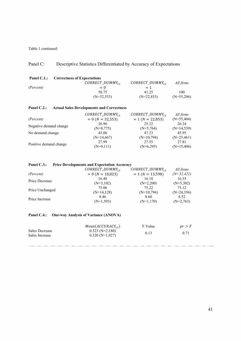
expectations prior to a change in demand and the development of actual sales. Descriptive

statistics are provided in Panel C of Table 1. _ , 1 implies that managers’

assessment of the development of demand over the next three months is equivalent to the actual

realization of demand.18 Panel C.1 shows that 41 percent of sales developments are correctly

anticipated. The column “all firms” in Panel C.2 indicates that approximately half of all

companies predicted a demand change and half of the companies correctly anticipated a stable

demand. Column “Correct dummy = 1” shows that, out of all correct expectations, 25.22 percent

refer to negative demand changes and 27.55 percent to positive demand changes. This result

suggests that the managers’ expectations are not strongly affected by overoptimism; otherwise,

we would expect to see only a significantly smaller proportion of correctly predicted negative

demand shocks.

Prices increased in 8.52 percent and decreased in 16.35 percent of all firm-month

observations (Panel C.3.).19 Thus, companies decrease prices more often than they increase them.

This is line with Cannon’s (2014) slippery price hypothesis, which predicts that prices tend to

become lower over time and implies that cost stickiness estimations can be influenced by

asymmetric price adjustments.20 These distributions are very similar for low accuracy (Correct

dummy = 0) and high accuracy (Correct dummy = 1).

                                                        

18 See Figure 3 for a detailed overview of possible cases. 19 Not all firms in the survey report price changes explaining the lower ‘N’ in Panel C.3 compared with Panels C.1 and C.2. 20 Specifically, companies’ price elasticity for demand decreases is greater than for demand increases because managers decrease prices to utilize existing capacity when demand falls, but increase capacity (instead of prices) when demand rises.

16   

In Panel C.4, we test whether the , in firm-years with a sales increase is

different from the , in firm-years with a sales decrease. The results indicate no

significant difference, providing further evidence that an optimism bias does not seem to be an

issue in the dataset.

Panel D of Table 1 presents the average level of capacity utilization differentiated by

sales decreases (D.1.) and sales increases (D.2.) as well as correctness of expectations. The

tabulated figures represent a much smaller proportion of the underlying dataset because capacity

utilization is surveyed only for manufacturing companies. The level of capacity utilization is

significantly higher when managers correctly anticipate future demand decreases. This result

supports nomological validity and suggests that our measure of accuracy is informative about

managerial decisions.

In an additional check for nomological validity, we calculate the correlation of

, with gross profit margin. The correlation is significantly positive (p < 0.05), which

is plausible because companies that can more accurately predict future demand can better meet

this demand and reduce idle capacity, thereby positively affecting the profit margin.

Taken together, the results provide confidence that our measure of expectation accuracy

is valid to capture the theoretical concept of interest.

Resource Adjustments

Our main regression model (2) is derived from the standard cost stickiness specification

introduced by Anderson et al. (2003) and the parameter estimates appear in the first column of

Table 2. For comparison, results of estimating model (2) conditional on expectation accuracy in

the whole sample and the reduced sample, respectively, are shown in the subsequent four

columns.

17   

Model (2) does not include additional control variables. is significantly positive

whereas is significantly negative in all specifications. Thus, costs are sticky on average. | |

is significantly higher (p < 0.01) for the low accuracy subsample than for the high accuracy

subsample. This holds for the whole sample as well as the reduced sample. Thus, the asymmetry

of the cost function is substantially higher in the low accuracy subsample ( = −0.25 for the

whole sample and = −0.33 for the reduced sample) than in the high accuracy subsample ( =

−0.09 for the whole sample and = −0.10 for the reduced sample). The results are also

economically significant. For example, in the high accuracy column (whole sample), an increase

of sales of 1 % is associated with a cost increase of 0.98 %. In contrast, a sales decrease of the

same magnitude (1 %) is associated with a cost decrease of 0.98 + (−0.09) = 0.89 % in the high

accuracy subsample, but only with a cost decrease of 1.07 + (−0.25) = 0.82 % in the low

accuracy subsample. Taken together, these results – statistically and economically – strongly

support our hypothesis that cost stickiness decreases when expectation accuracy is higher.

[Insert Table 2 about here]

Table 3 presents parameter estimates based on the full model (2’) that also controls for

differences in adjustment costs, industry, and capacity utilization. In line with our theoretical

predictions, the magnitude of cost stickiness decreases with an increase of expectation accuracy.

| | is significantly higher (p < 0.01) for the low accuracy subsample than for the high accuracy

subsample. The results are similar using the restricted sample that excludes 2007 and 2008

observations.

18   

Interestingly, cost stickiness is not supported in the high accuracy subsamples ( is not

significant). This challenges the cost stickiness hypothesis when managers can forecast future

demand accurately. In other words, high expectation accuracy seems to be a boundary condition

that had not been recognized in the cost stickiness literature before.

In accordance with Balakrishnan et al. (2004) results, parameter estimates show that cost

stickiness is more pronounced for companies with high capacity utilization ( is positively

significant).

[Insert Table 3 about here]

Price Adjustments

The following analyses investigate how price changes affect the estimation of sticky

costs. We start by estimating the standard model for cost stickiness as described in equation (2),

but differentiate between observations with price and without price changes.

[Insert Table 4 about here]

Table 4 shows the estimations for all observations in the first column of coefficients, the

subsample without price changes in the second column, and the estimations for the firm-year

observations with at least one month during which prices were adapted in the third column. In

both subsamples (with and without price changes), β2 is negative and significant.21 In line with

Cannon’s (2014) slippery price argument, the results show that the cost stickiness coefficient

                                                        

21 Excluding all firm-year observations from 2007 to 2008, (untabulated) results are identical.

19   

| | is lower in the sample with no price changes than in the sample with price changes. The

difference between the coefficients in the two subsamples is significant (p < 0.01), indicating

that cost stickiness studies using sales as proxy for activity may overestimate cost stickiness if

they do not control for price changes.

Next, we investigate whether our main results about the relationship between expectation

accuracy and cost stickiness hold when price effects are ruled out. Table 5 re-estimates our main

model, as shown in equation (2), for the subset of observations without selling price changes.

Similar to our results in Table 2 and Table 3, | | is larger for the subsamples with low

expectation accuracy. Moreover, costs are not sticky when managers’ expectation accuracy is

high and selling price changes are controlled for.

In sum, the results support our hypothesis even if price changes, a potential confounding

factor, are excluded.

[Insert Table 5 about here]

ADDITIONAL ANALYSES AND ROBUSTNESS CHECKS

Interplay among Cost Elasticity, Demand Volatility, and Accuracy of Expectations

According to Banker et al.’s (2014) findings, cost elasticity is lower for companies with

high demand volatility. This result is remarkable because it stands in contrast to the commonly

held belief that managers prefer more variable cost structures when uncertainty is higher. Banker

et al. argue that a decrease in cost elasticity reflects investments in fixed capacity to avoid

congestion when demand becomes high. The association between demand volatility and cost

behavior is modeled as follows (Banker et al. 2014):

20   

∆ln & , β , ∙ ∆lnSALES , ∙ , , (3)

where , ∙ _ , ∙ ,

We replicate this specification with our data. Table 6 presents the estimation results using model

(3), also differentiated by the direction of change in demand in the last two columns. Consistent

with Banker et al. (2014), higher demand volatility is associated with a more rigid cost structure.

22 is negative and significant for all observations and for demand increases. However, there is

no significant relation with demand decreases.23 This finding is in line with Banker et al.’s

theory, because the congestion of fixed inputs is not a problem when demand decreases.

[Insert Table 6 about here]

Our previous analyses have shown that the degree of managers’ forecast accuracy significantly

moderates the magnitude of cost stickiness. Because higher cost stickiness reflects lower cost

elasticity, cost elasticity should also be higher for expected demand decreases and lower for

unexpected demand decreases. This implies that the effect of demand volatility on cost elasticity

is also mitigated by the degree to which managers correctly anticipate a fall in demand.

Similarly, cost elasticity should be lower for expected demand increases than for unexpected

demand increases as managers are more willing to add or retain resources when they are

optimistic.

                                                        

22 In line with Banker et al. (2014), manufacturing companies are the reference group for all empirical tests. 23 When we exclude firm-year observations in 2007-2008, it does not alter our results.

21   

Banker et al.’s (2014) analyses are based on a formal model (see Appendix 2 for a short

summary) predicting a negative association between demand volatility and cost elasticity.24 We

extend the model by Banker et al. (2014) by showing that including down-side costs can alter

this conjecture in a decreasing market (see Appendix 2). The intuition for our result is that

demand volatility works symmetrically. When demand volatility increases it results in potentially

higher as well as lower sales. Thus, increasing demand volatility also results in a higher risk of

down-side costs (e.g., loss of investments in fixed capacity) due to the risk of lower expected

sales. Thus, we conjecture that managers who correctly anticipate a fall in demand prefer higher

cost elasticity.

In Banker et al.’s (2014) empirical tests, demand volatility is measured as the standard

deviation of the natural log-change in sales across all years for each firm. Based on our model

extension, we hypothesize that the theoretically negative association between demand volatility

and cost elasticity in Banker et al. (2014) becomes stronger (weaker) when managers accurately

expect that demand will increase (decrease). To test this prediction, model (3) is modified as

follows:

∆ln & , , ∙ ∆lnSALES , ∙ , ∙ , , (4)

where

, ∙ _ , ∙ _ , ∙ , ∙ ,

                                                        

24 In Appendix 2, we refer to the concept of demand uncertainty, similar to Banker et al. (2014). In our empirical part we prefer to use the term “demand volatility” because it describes what our study and Banker et al. (2014) actually measure more precisely.

22   

Table 7 presents the estimation results using model (4). For the overall sample, the results

are very similar to model 3, the replication of Banker et al. (2014). However, when the analysis

is conducted separately for demand increases and demand decreases, the results indicate that

expectation accuracy moderates the relation between demand volatility and cost elasticity.

Specifically, in line with the predictions from the extension of the theoretical model in Appendix

2, expectation accuracy strengthens the negative effect of demand volatility on cost elasticity in

the subsample of demand increases 0 but mitigates the effect for the subsample of

demand decreases 0 .25 This confirms our hypothesis that the relationship between

demand volatility and cost behavior depends on the accuracy of managers’ expectations for

changing demand. Thus, if a sample is dominated by demand decreases, the association between

demand volatility and costs becomes stronger with increasing expectation accuracy. This makes

sense because managers who correctly anticipate a negative demand shock will be prepared to

cut costs even more when higher volatility represents a greater risk. However, if a sample is

dominated by demand increases, the effect of managerial expectation accuracy further

strengthens the negative association between demand volatility and cost elasticity. This is

plausible because it implies that potential congestion costs can be reduced.

[Insert Table 7 about here]

These results contribute to reconciling the conflicting findings in the literature regarding the

association between demand volatility and cost elasticity. Specifically, Banker et al. (2014) show

that costs elasticity is decreasing in demand volatility whereas Holzhacker et al. (2015) conclude

                                                        

25 Exclusion of financial crisis (years 2007-2008) firm-year observations does not change our results.

23   

that firms will alter their procurement choices to increase cost elasticity in response to high

uncertainty. Because the latter study is based on a sample of hospitals, Holzhacker et al. (2015)

argue that the difference in results might stem from diverging management incentives and

ownership structure compared with public firms, as in Banker et al.’s setting. Our analysis

suggests an additional potential explanation. The results show that cost behavior is particularly

determined by the accuracy of managers’ expectations about future demand. Thus, the difference

between the previous studies is explained by managers’ capacity adjustment decisions depending

on whether they can correctly anticipate a positive or negative demand shock. Notably, the

settings of Holzhacker et al. (2015) and Banker et al. (2014) indeed differ with respect to demand

growth. Banker et al. (2014) analyze manufacturing firms from 1979–2008, a period in which

output roughly doubled (Nutting 2016). In contrast, the hospital industry in Holzhacker et al.’s

setting exhibited a relatively steady decline (measured as patient days).

Combining our results with the previous studies yields the following interpretation. In

growing markets, managers of companies with higher demand volatility prefer less elastic cost

structures (i.e., a higher ratio of fixed to variable costs) than managers of companies with lower

volatility. This result is in line with the motivation to avoid congestion costs when demand

suddenly increases. However, among those managers who operate in environments with

decreasing demand and who accurately predict the decline, the managers of companies with

higher volatility strive for higher cost elasticity compared to managers of companies with lower

volatility. Future research could further test our explanation by comparing different industries

and periods that differ regarding expected forecast accuracy and the frequency of demand

decreases.

24   

Robustness Checks

Managerial Incentives to Meet or Beat the Zero-Earnings Benchmark

Companies have an incentive to report healthy earnings to avoid negative consequences.

These could be related to a greater intervention by banks due to the violation of debt contracts,

prevention of dividend payments and cash bonuses, or the issuance of going-concern opinions.

Thus, executives are inclined to manage costs to meet or beat the zero-earnings benchmark. To

realize necessary cost reductions, firms reporting small profits are more likely to dismiss blue-

collar workers when demand decreases and increase hours (instead of employees) when demand

increases (Dierynck et al. 2012). On average, this leads to a reduction in the level of cost

stickiness.26

To verify that previous estimates in Table 3 are not driven by managerial incentives to

meet or beat the zero-earnings benchmark, results are subjected to two robustness tests. First,

regression estimates are obtained based on a subsample by excluding firm-year observations with

small profits. Second, model (2’) is estimated with an additional control variable capturing the

effect of small profit firms. This approach follows Dierynck et al. (2012), who select small profit

firms using a dummy variable set to one if the net income scaled by total assets is greater than or

equal to zero but less than 1 percent. Untabulated results of both tests show that previous

findings remain substantially similar.

Ownership Structure

Apart from the high accuracy of managerial expectations, a lower level of cost stickiness

can also result from differences in the ownership structure across companies in the sample.

                                                        

26 Other studies test the impact of managerial incentives on cost behavior by investigating the effect of meeting earnings targets or managerial empire building (Chen, Lu, and Sougiannis 2012; Kama and Weiss 2013).

25   

Capital market pressure and managerial compensation tied to stock performance have been

identified as sources of short-termism that induce managers of public companies to avoid

reporting losses or meet or beat analysts’ forecasts (Bhojraj and Libby 2005; Degeorge et al.

1999; Roychowdhury 2006). In contrast, the large proportion of family ownership in private

firms can lead to an alignment effect that incentivizes long-term strategies over short-term

benefits to preserve family reputation (Bennedsen et al. 2007; Chen et al. 2008). Therefore, in

another robustness check, model (2’) in Table 3 is extended by the moderation of a dummy

variable that is equal to one if the company is public and zero otherwise. Untabulated results

remain unchanged.

Additional Cost Categories

In addition to SG&A costs, we re-run model (2’) using the change in total operating costs

as dependent variable in Table 3. The behavior of cost of goods sold is not examined because

changes in inventories prevent stickiness of cost of goods sold. Thus, accuracy of managerial

expectations is not expected to have a significant effect on this cost category. Overall,

untabulated results support the hypothesis that the accuracy of managerial expectations

determines not only SG&A cost behavior, but also the change in total operating costs.

Accuracy and Endogeneity

Our theory and empirical tests focus on conditional effects (e.g., the cost function

conditional upon demand increase vs. demand decrease as well as the cost asymmetry

conditional upon expectation accuracy). Such relations are less prone to endogeneity concerns

than main effects in regressions.27

                                                        

27 The method literature suggests using interaction specifications as one statistical remedy to alleviate endogeneity concerns since “simulation findings of Evans (1985) and a proof by Siemsen et al. (2010), … demonstrate that

26   

In most of our analyses, we split the sample in a low and a high accuracy subsamples. In

additional (untabulated) robustness checks, we re-estimate all specifications using a three-way

interaction of ∆lnSALES , , the decrease indicator variable , , and a continuous measure of

, . All results are robust in these alternative specifications.

Moreover, we address potential endogeneity issues in those specifications where

, is included as a right hand variable by following a similar two-stage OLS

procedure as Patatoukas (2012). In the first stage, we regress , on the firm-specific

variables size (natural log of total assets), age (difference between the firm’s financial year end

and founding year), _ , and a dummy variable indicating whether the firm is

publicly listed or not. Large firms can invest more in forecasting technology (size), older firms

likely have more knowledge about their business (age), it is potentially more difficult to forecast

future demand accurately in high demand volatility environments ( _ ), and

publicly listed firms may be under more pressure to grow (listed). We also add firm-, industry-,

and time-fixed effects as well as geographic-fixed effects. The latter controls for local trends.

In the second stage, we rerun all our regressions with , , but now with the

residuals from the first stage instead of , . The untabulated results are very similar.

Taken together, endogeneity is likely not a concern for our results.

CONCLUSION

This study uses a Danish dataset combining financial statement information with a

business survey initiated by a European Union program to investigate the interplay between the

accuracy of managers’ demand expectations and SG&A cost behavior. Other researchers have

                                                                                                                                                                                

although method bias can inflate (or deflate) bivariate linear relationships, it cannot inflate (but does deflate) quadratic and interaction effects” (Podsakoff et al. 2012, 564).

27   

shown that cost behavior is driven by deliberate resource adjustment decisions to avoid

adjustment costs associated with adapting resource levels. The level of capacity utilization is

considered the outcome of these decisions (e.g., Anderson et al. 2003; Anderson et al. 2007;

Balakrishnan et al. 2004; Kama and Weiss 2013). Extending this line of reasoning, we

hypothesized that the accuracy of managerial expectations is an important predictor of cost

behavior. Results show that, when a fall in demand was accurately expected, managers

successfully cut capacity, resulting in a significant decrease in SG&A cost stickiness compared

to firms that did not correctly anticipate a change in demand.

Moreover, the study assesses the effect of selling price changes on cost stickiness

estimations. Analyzing the traditional cost stickiness specification separately for firm-years with

selling price changes and firm-years without selling price changes indicates that the cost

stickiness estimate is significantly lower when confounding effects of price changes are ruled

out. Thus, studies using sales as a proxy for volume might overestimate cost stickiness if they

cannot control for price changes.

Subsequently, the study reanalyzes the association between expectation accuracy and cost

stickiness for the sub-sample of firm-years without price changes. The analyses suggest that the

main findings in this paper are robust to potential confounding effects of price changes. Even

when ruling out selling price effects, the cost stickiness is stronger for those firm-years with low

expectation accuracy compared to those with high accuracy.

Finally, additional analyses are conducted to test if the accuracy of managerial

expectations moderates the association between demand volatility and cost behavior. Extending

the analytical model as well as the empirical specifications introduced by Banker et al. (2014),

our study demonstrates that the relationship is negative for unexpected demand decreases but

28   

positive for expected demand decreases. These results help reconcile contradictory findings in

the literature that suggest that cost variability is either positively (Holzhacker et al. 2015) or

negatively (Banker et al. 2014) related to demand volatility.

All analyses in this study were conducted using data from Danish companies.

Consequently, empirical estimates are not influenced by national differences in labor laws,

market conditions, etc. Future studies should assess the generalizability of our findings to other

contexts. In addition, although the consideration of selling prices as a potential confounding

variable is a contribution of this study, the categorical nature of the survey data does not allow

for the measurement of the magnitude of price changes in response to expected or unexpected

demand changes. Furthermore, the argument underlying the main hypothesis implies that

adjustment costs occur within the time frame of the empirical tests. However, it is possible that

some adjustment costs (e.g., negative effects on company reputation or working atmosphere)

arise with a time lag and are not captured by the empirical tests. Overcoming these limitations

would be a valuable contribution for future research. Moreover, this study shows how

managerial expectations impact cost structures, but it does not provide insights into how

managers derive expectations about future demand. The investigation of these factors, such as

personal characteristics, analyses, and decision-making processes, and their relation to resource

adjustment and cost behavior is left to future research.

29   

Appendix 1

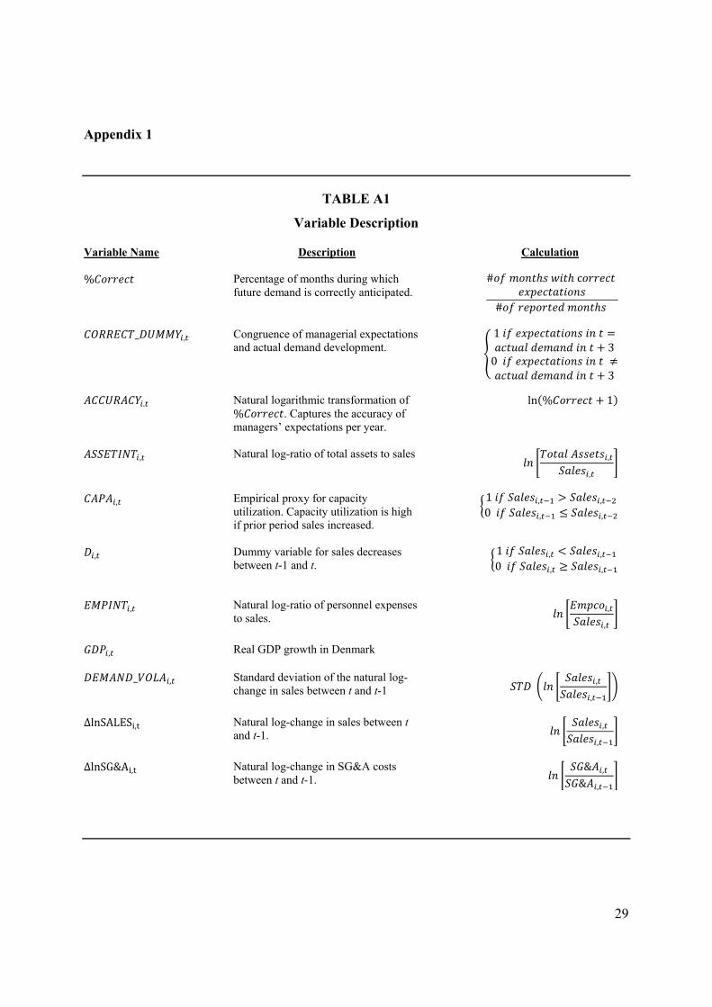
TABLE A1

Variable Description

Variable Name Description Calculation

% Percentage of months during which future demand is correctly anticipated.

# c

#

_ , Congruence of managerial expectations and actual demand development.

1 3

0 3

. Natural logarithmic transformation of % . Captures the accuracy of managers’ expectations per year.

ln % 1

, Natural log-ratio of total assets to sales ,

,

, Empirical proxy for capacity utilization. Capacity utilization is high if prior period sales increased.

1 , ,

0 , ,

, Dummy variable for sales decreases between t-1 and t.

1 , ,

0 , ,

, Natural log-ratio of personnel expenses to sales.

,

,

, Real GDP growth in Denmark

_ , Standard deviation of the natural log-change in sales between t and t-1 ,

,

∆lnSALES , Natural log-change in sales between t and t-1.

,

,

∆lnSG&A , Natural log-change in SG&A costs between t and t-1.

& ,

& ,

30   

TABLE A2

Excerpt from the Questionnaire of the Joint Harmonized EU Program of Business and

Consumer Surveys

Expression

Question Answer possibilities

Expectations How do you expect demand (sales) to change over the next three months?

Increase Remain Unchanged Deteriorate

Actual Demand How did demand (sales) change over the past three months?

Increased Remained Unchanged Deteriorated

Prices How did the prices you charged change over the past three months?

Increased Remained Unchanged Deteriorated

Capacity Utilization28 At what capacity is your company currently operating (as a percentage of full capacity)?

Percent

In the survey, specifically see Section 2.2. and subsections 1-2 and 4-6 in Annex 2

(http://ec.europa.eu/economy_finance/db_indicators/surveys/documents/bcs_user_guide_en.pdf)

                                                        

28 Question is included in the survey for manufacturing companies only.

31   

Appendix 2: Summary and Extension of Banker et al.’s (2014) model

In their 2015 AAA award-winning paper, Banker et al. (2014) show that higher demand

uncertainty (higher variance of demand) results in a more rigid cost structure (more fixed and

less variable inputs), challenging the conventional wisdom (i.e., lower fixed and higher variable

costs). However, Banker et al. (2014) do not model the down-side costs of, e.g., bankruptcy.

Although it is plausible that fixed inputs are the bottleneck when demand increases, we

conjecture that the risk of bankruptcy alters the managers’ cost behavior in a decreasing market.

When demand decreases the risk of bankruptcy increases and (as a result) managers prefer a less

rigid cost structure. Following this line of reasoning, we first derive the analytical result in

Banker et al. (2014) making a few simplifying assumptions to reduce the mathematical

complexity.

Banker et al. (2014) study the resource allocation in a risk-neutral firm facing uncertain

demand. That is, the firm wants to minimize the total cost subject to a given production

technology , :

min , . . , (A1)

where denotes the fixed (variable) input for producing output and is the input

price.

We assume that the firm’s technology is given by a Cobb-Douglas production function:

, (A2)

32   

where (without loss of generality) ½.

As the firm chooses fixed input x prior to actual demand is known and variable input z is

chosen after observing realized demand, the optimal level of variable input z is:

(A3)

Substitution of the optimal level of variable input z into the firm’s cost problem yields:

Min Min (A4)

In their model, Banker et al. (2014) assume there are no inventories, firms always fully

meet the demand , and the distribution of demanded quantity follows a normal

distribution:

~ , (A5)

where denotes the mean level of demand (demand uncertainty).

Keeping in mind, that Banker et al. (2014) study how demand uncertainty relates to

cost behavior. By definition the variance of output is given by:

(A6)

Thus, substitution of the variance of output into equation (A4) yields:

33   

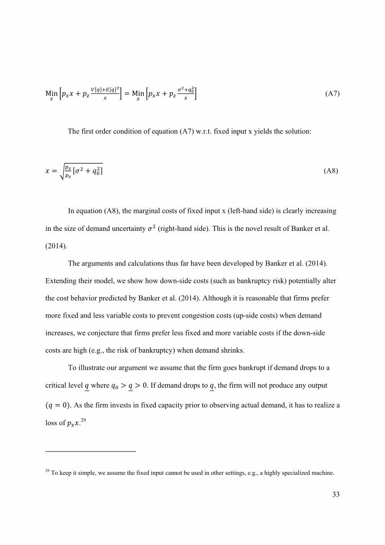
Min Min (A7)

The first order condition of equation (A7) w.r.t. fixed input x yields the solution:

(A8)

In equation (A8), the marginal costs of fixed input x (left-hand side) is clearly increasing

in the size of demand uncertainty (right-hand side). This is the novel result of Banker et al.

(2014).

The arguments and calculations thus far have been developed by Banker et al. (2014).

Extending their model, we show how down-side costs (such as bankruptcy risk) potentially alter

the cost behavior predicted by Banker et al. (2014). Although it is reasonable that firms prefer

more fixed and less variable costs to prevent congestion costs (up-side costs) when demand

increases, we conjecture that firms prefer less fixed and more variable costs if the down-side

costs are high (e.g., the risk of bankruptcy) when demand shrinks.

To illustrate our argument we assume that the firm goes bankrupt if demand drops to a

critical level where 0. If demand drops to , the firm will not produce any output

0 . As the firm invests in fixed capacity prior to observing actual demand, it has to realize a

loss of .29

                                                        

29 To keep it simple, we assume the fixed input cannot be used in other settings, e.g., a highly specialized machine.

34   

Next, we relate the probabilities of different outcomes of demand by the cumulative

distribution function . Thus, let and 1 denote the risk of

bankruptcy and the probability of “going concern”, respectively.

Now the equivalent of the firm’s cost problem in equation (A1) can be formalized as

follows:

min , 1

. .

. . , (A9)

Given the same assumptions as in equations (A2) and (A5), the equivalent expression of

equation (A7) is:

Min 1 (A10)

Again, we take the first order condition of equation (A10) w.r.t. fixed input x which

yields the solution:

1. .

(A11)

Based on equation (A11), it is clear that the risk of bankruptcy reduces the

required units of fixed resources x (right-hand side) to restore optimum. That is, the cost

35   

elasticity is decreasing in the risk of bankruptcy . Figure 4 illustrates how demand

uncertainty is related to the risk of bankruptcy . When demand uncertainty

increases the risk of bankruptcy also increases for a given critical level .

Accordingly, we derive our empirical prediction when demand uncertainty increases.

If the risk of bankruptcy 0 in equation (A11) then fixed input x is only

influenced by demand uncertainty . This is equivalent to equation (A8). However the

introduction of bankruptcy risk in equation (A11) moderates the predictions in equation (A8).

When demand uncertainty increases the risk of bankruptcy also increases cf.

figure 4. Thus, 1 becomes higher but the increase is smaller than in equation

(A8). However, the right-hand side of equation (A11) also drops by when

demand uncertainty increases. Thus, higher demand uncertainty can result in less fixed

input x if 1 or .30 The intuition for

our prediction is that the (expected) demanded quantity (in Banker et al., 2014) now drops

with the (expected) loss of bankruptcy which is increasing in demand uncertainty .

                                                        

30 By definition, we also require that where 0; 0.5 . Thus, the inequality only holds if

1 . When approaches zero (0.5) the costs of bankruptcy decreases (increases) and (as a result) the

inequality is less (more) likely to hold. Consider figure 4, the intuition is that when the critical

level of output approaches zero the risk of bankruptcy vanishes whereas it increases when gets closer to .

Thus, it is easier to fulfill the inequality for a high critical level of output . Naturally, the initial size of also

matters.

36   

Taken together, our analysis shows how Banker et al.’s (2014) framework yields

different predictions depending on whether managers expect higher or lower future demand. The

implications regarding the association between demand volatility and cost elasticity derived from

this simple model extension are in line with our empirical findings.

37   

References

Amore, M. D., and M. Bennedsen. 2013. The value of local political connections in a low-corruption environment. Journal of Financial Economics 110 (2):387-402.

Anderson, M., R. Banker, R. Huang, and S. Janakiraman. 2007. Cost behavior and fundamental analysis of SG&A costs. Journal of Accounting, Auditing & Finance 22 (1):1-28.

Anderson, M., R. Banker, and S. Janakiraman. 2003. Are selling, general, and administrative costs "sticky"? Journal of Accounting Research 41 (1):47-63.

Anderson, S., and W. Lanen. 2009. Understanding cost management: What can we learn from the empirical evidence on sticky costs? Working paper.

Balakrishnan, R., and T. S. Gruca. 2008. Cost stickiness and core competency: A note. Contemporary Accounting Research 25 (4):993-1006.

Balakrishnan, R., E. Labro, and N. Soderstrom. 2014. Cost structure and sticky costs. Journal of Management Accounting Research 26 (2):91-116.

Balakrishnan, R., M. Petersen, and N. Soderstrom. 2004. Does capacity utilization affect the stickiness of cost? Journal of Accounting, Auditing & Finance 19 (3):283-300.

Banker, R., and D. Byzalov. 2014. Asymmetric cost behavior. Journal of Management Accounting Research 26 (2):43-79.

Banker, R., D. Byzalov, and J. Plehn-Dujowich. 2014. Demand uncertainty and cost behavior. The Accounting Review 89 (3):839-865.

Banker, R., D. Byzalov, and L. Threinen. 2013a. Determinants of international differences in asymmetric cost behavior. Working paper, Temple University.

Banker, R., S. Fang, and M. Metha. 2013b. Anomalous financial performance ratios during economic downturns. Working paper, Temple University.

Bennedsen, M., K. M. Nielsen, F. Pérez-González, and D. Wolfenzon. 2007. Inside the family firm: The role of families in succession decisions and performance. The Quarterly Journal of Economics 122 (2):647-691.

Bentolila, S., and G. Bertola. 1990. Firing costs and labour demand: How bad is eurosclerosis? The Review of Economic Studies 57 (3):381-402.

Bhojraj, S., and R. Libby. 2005. Capital market pressure, disclosure frequency-induced earnings/cash flow conflict, and managerial myopia. The Accounting Review 80 (1):1-20.

Cannon, J. 2014. Determinants of ''sticky costs'': An analysis of cost behavior using United States air transportation industry data. The Accounting Review 89 (5):1645-1672.

Chen, C., T. Gores, and J. Nasev. 2013. Managerial overconfidence and cost stickiness. Working paper.

Chen, C., H. Lu, and T. Sougiannis. 2012. The agency problem, corporate governance, and the asymmetrical behavior of selling, general, and administrative costs. Contemporary Accounting Research 29 (1):252-282.

Chen, J., I. Kama, and R. Lehavy. 2015. Management expectations and asymmetric cost behavior. Working paper, Ross School of Business, University of Michigan.

Chen, S., X. Chen, and Q. Cheng. 2008. Do family firms provide more or less voluntary disclosure? Journal of Accounting Research 46 (3):499-536.

38   

Dahl, M. S., C. L. Dezső, and D. G. Ross. 2012. Fatherhood and managerial style: How a male CEO’s children affect the wages of his employees. Administrative Science Quarterly 57 (4):669-693.

Dahl, M. S., and O. Sorenson. 2012. Home sweet home: Entrepreneurs' location choices and the performance of their ventures. Management Science 58 (6):1059-1071.

Degeorge, F., J. Patel, and R. Zeckhauser. 1999. Earnings management to exceed thresholds. The Journal of Business 72 (1):1-33.

Dierynck, B., W. Landsman, and A. Renders. 2012. Do managerial incentives drive cost behavior? Evidence about the role of the zero earnings benchmark for labor cost behavior in private belgian firms. The Accounting Review 87 (4):1219-1246.

European Commission. 2014. The joint harmonised EU programme of business and consumer surveys. Brussels: Directorate-General for Economic and Financial Affairs.

Evans, M. G. 1985. Monte carlo study of the effects of correlated method variance in moderated multiple regression analysis. Organizational Behavior and Human Decision Processes 36 (3):305-323.

Goex, F. 2002. Capacity planning and pricing under uncertainty. Journal of Management Accounting Research 14:59.

Hamermesh, D. 1993. Labour demand. Princeton, N.J.: Princeton University Press. Hamermesh, D., and G. Pfann. 1996. Adjustment costs in factor demand. Journal of Economic

Literature 34 (3):1264-1292. Hayashi, F. 1982. Tobin's marginal q and average q: A neoclassical interpretation. Econometrica

50 (1):213-224. Holzhacker, M., R. Krishnan, and M. Mahlendorf. 2015. Unraveling the black box of cost

behavior: An empirical investigation of risk drivers, managerial resource procurement, and cost elasticity. The Accounting Review 90 (6):2305-2335.

Horngren, C., M. Datar Srikant, and V. Rajan Madhav. 2015. Cost accounting: A managerial emphasis. 15 ed. Global edition. Harlow, Essex, England: Pearson.

Kama, I., and D. Weiss. 2013. Do earnings targets and managerial incentives affect sticky costs? Journal of Accounting Research 51 (1):201-224.

Mankiw, G. 1985. Small menu costs and large business cycles: A macroeconomic model of monopoly. The Quarterly Journal of Economics 100 (2):529-537.

Noreen, E. 1991. Conditions under which activity-based cost systems provide relevant costs. Journal of Management Accounting Research 3 (4):159-168.

Nutting, R. 2017. Think nothing is made in America? Output has doubled in three decades 2016 [cited July 18 2017]. Available from http://www.marketwatch.com/story/us-manufacturing-dead-output-has-doubled-in-three-decades-2016-03-28.

Patatoukas, P. N. 2012. Customer-base concentration: Implications for firm performance and capital markets. The Accounting Review 87 (2):363-392.

Podsakoff, P. M., S. B. MacKenzie, and N. P. Podsakoff. 2012. Sources of method bias in social science research and recommendations on how to control it. Annual Review of Psychology 63:539-569.

Rotemberg, J. 1982. Sticky prices in the United States. Journal of Political Economy 90 (6):1187-1211.

Roychowdhury, S. 2006. Earnings management through real activities manipulation. Journal of Accounting and Economics 42 (3):335-370.

39   

Siemsen, E., A. Roth, and P. Oliveira. 2010. Common method bias in regression models with linear, quadratic, and interaction effects. Organizational Research Methods 13 (3):456–476.

Varian, H. R. 1992. Microeconomic analysis. 3rd ed. New York, NY: Norton. Venieris, G., V. Naoum, and O. Vlismas. 2015. Organisation capital and sticky behaviour of

selling, general and administrative expenses. Management Accounting Research 26:54-82.

Weiss, D. 2010. Cost behavior and analysts' earnings forecasts. The Accounting Review 85 (4):1441-1471.

40   

Tables

TABLE 1

Descriptive Statistics

Panel A: Descriptive Statistics in Million DKK (Million USD, exchange rates in year 2000)

N Mean

Standard Deviation

Lower Quartile Median

Upper Quartile

Sales [1] 4,107 453.26 (57.16)

1,703.08 (214.76)

42.57 (5.37)

133.39 (16.82)

346.65 (43.71)

SG&A costs [2] 4,107 101.52 (12.80)

347.05 (43.76)

10.96 (1.38)

28.26 (3.56)

72.97 (9.20)

Personnel expenses [3] 4,068 104.45 (13.17)

335.03 (42.25)

14.22 (1.79)

35.86 (4.52)

82.25 (10.37)

SG&A costs/ Sales [4] 4,107 0.32 0.25 0.14 0.26 0.45 EMPINT [5] 4,068 0.34 0.24 0.20 0.30 0.43

ASSETINT [6] 4,107 0.80 0.94 0.43 0.62 0.87 Number of Employees [7] 3,996 559.13 1,795.31 81.00 213.00 464.50

∆ln & , [8] 4,107 0.02 0.55 -0.36 -0.00 0.34 ACCURACY [9] 4,107 0.32 0.26 0.00 0.41 0.51

DEMAND_VOLA [10] 4,107 0.51 0.16 0.43 0.48 0.56

GDP [11] 4,107 0.88 2.25 0.39 0.82 2.44

Panel B: Pearson Correlation

[1] [2] [3] [4] [5] [6] [7] [8] [9] [10]

[1] Sales [2] SG&A costs 0.68*** [3] Personnel

expenses 0.86*** 0.84***

[4] SG&A costs/ Sales

-0.11*** 0.11*** -0.03

[5] EMPINT -0.12*** -0.03* -0.02 0.50*** [6] ASSETINT -0.01 0.01 0.01 0.03** 0.10***

[7] Number of Employees

0.82*** 0.71*** 0.90*** -0.05*** -0.05*** 0.01

[8] ∆ln & , 0.08*** 0.10*** 0.10*** 0.07*** 0.03* -0.03* 0.03** [9] ACCURACY -0.02 -0.03* -0.04** -0.03** -0.03* -0.00 -0.02 -0.01 [10] DEMAND_

VOLA -0.01 0.03** 0.02 0.10*** 0.06*** 0.08*** 0.00 -0.01 -0.04**

[11] GDP -0.05*** -0.05*** -0.06*** -0.03** -0.03* 0.00 -0.02 -0.33*** 0.02 -0.05***

41   

Table 1 continued:

Panel C: Descriptive Statistics Differentiated by Accuracy of Expectations Panel C.1.: Correctness of Expectations

(Percent)

_ ,

0 _ ,

1 All firms

58.75

(N=32,553) 41.25

(N=22,853) 100

(N=55,206)

Panel C.2.: Actual Sales Developments and Correctness

(Percent)

_ ,

0 32,553 _ ,

1 22,853 All firms

(N=55,404)

Negative demand change 26.96

(N=8,775) 25.22

(N=5,764) 26.24

(N=14,539)

No demand change 45.06

(N=14,667) 47.23

(N=10,794) 45.95

(N=25,461)

Positive demand change 27.99

(N=9,111) 27.55

(N=6,295) 27.81

(N=15,406) Panel C.3.: Price Developments and Expectation Accuracy (Percent)

_ ,

0 18,823 _ ,

1 13,598 All firms

(N=32,421)

Price Decrease 16.48

(N=3,102) 16.18

(N=2,200) 16.35

(N=5,302)

Price Unchanged 75.06

(N=14,128)75.22

(N=10,794)75.12

(N=24,356)

Price Increase 8.46

(N=1,593) 8.60

(N=1,170) 8.52

(N=2,763) Panel C.4.: One-way Analysis of Variance (ANOVA)

. F Value Sales Decrease 0.323 (N=2,180)

0.13 0.71 Sales Increase 0.320 (N=1,927)

42   

Table 1 continued:

Panel D: Average Level of Capacity Utilization for Manufacturing Companies (monthly)

Panel D.1.: Demand Decrease (Percent)

_ ,

0 613 _ ,

1 422

F-test for Difference

Capacity utilization 70.11 72.87 **

Panel D.2.: Demand Increase (Percent)

_ ,

0 685 _ ,

1 516

F-test for Difference

Capacity utilization 77.93 78.48

∗ of 0.10, ∗∗ of 0.05, ∗∗∗ of 0.01 (F-tests). *,**, and *** indicate significance at the 10, 5, and 1 percent levels, respectively. See Table A1 in Appendix 1 for a description of all variables.

_ , captures the congruence between managerial expectations about future demand and actual demand on a monthly basis. _ , 1 if the manager’s expectation in t is equivalent to the actual change in demand in t+3. The difference is three months because the survey asks for the expected change in demand for the next three months and the actual development of demand over the past three months. See Figure for an overview of all possible cases.

. is the mean annual level of log % 1 with % # /# . The level of capacity utilization is retrieved from the survey questionnaire for manufacturing companies. See Table A1 in Appendix 1 for the description of the variable.

43   

TABLE 2

Cost Stickiness Estimations Conditional upon Expectation Accuracy, Model (2)

Model (2) ∆ln & , β , ∙ ∆lnSALES , ∙ , , , where , ∙ ,

Whole Samplea

Whole Samplea

Reduced Sampleb

High Accuracy

Low Accuracy

High Accuracy

Low Accuracy

Coeff. Variable Pred. Sign

Estimate (t-statistic)

Estimate

(t-statistic) Estimate

(t-statistic)

Estimate

(t-statistic) Estimate

(t-statistic)

Intercept -0.05*** (-4.22)

-0.03** (-2.32)

-0.06***(-3.73)

-0.05** (-2.27)

-0.08*** (-4.48)

∆ , + 1.02***(45.37)

0.98***(27.35)

1.07***(38.93)

0.98*** (25.71)

1.09*** (37.61)

, ∙ ∆ , − -0.17***(-4.74)

-0.09** (-1.79)

-0.25***(-4.89)

-0.10* (-1.61)

-0.33*** (-4.73)

, -0.01 (-0.87)

-0.01 (-0.52)

-0.02 (-0.75)

-0.00 (-0.16)

-0.01 (-0.38)

, no no no no no

n 4,107 2,064 2,043 1,707 1,710

Adj. R2 0.67 0.67 0.71 0.59 0.68

a Whole sample, including all firm-year observations between 1999 and 2013. b Reduced sample includes all firm-year observations between 1999 and 2013, excluding firm-year observations from 2007 and 2008. *,**, and *** indicate one-sided significance at the 10, 5, and 1 percent levels, respectively. The numbers in parentheses are the t-statistics, based on standard errors clustered by firm and year. High Accuracy (Low Accuracy) denotes the subsample above (below) the median (i.e., the 50th percentile) of ACCURACY. See Table A1 in Appendix 1 for a description of all variables.

44   

TABLE 3

Cost Stickiness Estimations Conditional upon Expectation Accuracy, Model (2’)

Model (2’):

∆ln & , β , ∙ ∆lnSALES , ∙ , ∙ , , ,

where , ∙ , ∙ , ∙ ,

Panel A: Whole Samplea Model (2’)

Not controlling for capacity utilization

Controlling for capacity utilization

High

Accuracy Low

Accuracy High

Accuracy Low

Accuracy

Coeff. Variable Pred. Sign

Estimate (t-statistic)

Estimate (t-statistic)

Estimate (t-statistic)

Estimate (t-statistic)

Intercept 0.03 (0.93)

-0.03 (-1.05)

0.04 (1.01)

-0.05* (-1.58)

∆ , + 0.98*** (26.42)

1.06*** (38.77)

0.98*** (25.81)

1.06*** (37.26)

, ∙ ∆ , 0.03 (0.30)

-0.27*** (-3.05)

-0.11 (-0.82)

-0.52*** (-2.86)

, -0.02 (-0.68)

-0.03 (-1.00)

-0.04 (-1.28)

-0.04* (-1.47)

Controls

, ∙ ∆lnSALES , ∙ ,

0.07* (1.45)

-0.03 (-0.76)

0.08* (1.59)

-0.03 (-0.70)

,

0.04** (2.06)

0.02 (1.22)

0.04** (1.87)

0.01 (0.49)

, ∙ ∆lnSALES , ∙ ,

0.01 (0.59)

-0.04 (-0.13)

0.02 (0.79)

-0.00 (-0.09)

, 0.01 (0.64)

-0.02* (-1.32)

0.00 (0.09)

-0.02* (-1.53)

, ∙ ∆lnSALES , ∙ ,

0.16** (1.67)

0.25* (1.60)

,

-0.01 (-0.68)

0.00 (0.05)

Industry slope and main effect

yes yes yes yes

n

2,042 2,022 1,862 1,826

Adj. R2

0.63 0.71 0.65 0.72

45   

Table 3 continued:

Panel B: Reduced Sampleb Model (2’)

Not controlling for capacity utilization

Controlling for capacity utilization

High

Accuracy Low

Accuracy High

Accuracy Low

Accuracy

Coeff. Variable Pred. Sign

Estimate (t-statistic)

Estimate (t-statistic)

Estimate (t-statistic)

Estimate (t-statistic)

Intercept 0.03 (0.77)

-0.05* (-1.58)

0.04 (0.87)

-0.08** (-2.14)

∆ , + 0.99*** (24.83)

1.09*** (37.29)

0.99*** (24.22)

1.09*** (35.56)

, ∙ ∆ , 0.07 (0.47)

-0.33*** (-2.73)

-0.22 (-1.08)

-0.87*** (-3.20)

, -0.00 (-0.10)

-0.02 (-0.72)

-0.04 (-1.10)

-0.06** (-1.66)

Controls

, ∙ ∆lnSALES , ∙ ,

0.05 (0.68)

-0.01 (-0.19)

0.06 (0.88)

-0.03 (-0.48)

,

0.05** (2.10)

0.02 (1.04)

0.05** (1.91)

0.00 (0.22)

, ∙ ∆lnSALES , ∙ ,

-0.02 (-0.88)

-0.00 (-0.11)

-0.02 (-0.85)

-0.00 (-0.02)

,

0.00 (0.22)

-0.02 (-1.18)

-0.01 (-0.33)

-0.02* (-1.40)

, ∙ ∆lnSALES , ∙ ,

0.32** (2.20)

0.51** (2.31)

,

-0.02 (-0.68)

-0.00 (-0.00)

Industry slope and main effect

yes yes yes yes

n

1,691 1,693 1,517 1,507

Adj. R2 0.59 0.69 0.61 0.70

a Whole sample, including all firm-year observations between 1999 and 2013. b Reduced sample includes all firm-year observations between 1999 and 2013, excluding firm-year observations from 2007 and 2008.

*,**, and *** indicate one-sided significance at the 10, 5, and 1 percent levels, respectively. The numbers in parentheses are the t-statistics, based on standard errors clustered by firm and year.

The following control variables , are included as both fixed effects as well as interaction effects: employee intensity , , asset intensity , , industry classification , and the empirical proxy for capacity utilization , .

High Accuracy (Low Accuracy) denotes the subsample above (below) the median (i.e., the 50th percentile) of ACCURACY.

See Table A1 in Appendix 1 for a description of all variables.

46   

TABLE 4

Selling Price Changes and the Standard Estimation of Cost Stickiness

Model (2) ∆ln & , β , ∙ ∆lnSALES , ∙ , , , where , ∙ ,

All

observations No price changes

With price changes

Coeff. Variable Pred. Sign

Estimate (t-statistic)

Estimate (t-statistic)

Estimate (t-statistic)

Intercept -0.06*** (-4.05)

-0.08*** (-3.27)

-0.05*** (-2.70)

∆ , + 1.04*** (33.94)

1.00*** (17.20)

1.06*** (29.40)

, ∙ ∆ , -0.21*** (-4.36)

-0.16** (-1.93)

-0.23*** (-3.93)

, -0.00

(-0.22) 0.01

(0.30) -0.01

(-0.47) n 2,798 873 1,925

Adj. R2 0.62 0.59 0.63

*,**, and *** indicate one-sided significance at the 10, 5, and 1 percent levels, respectively. The numbers in parentheses are the t-statistics, based on standard errors clustered by firm and year. See Table A1 in Appendix 1 for a description of all variables.

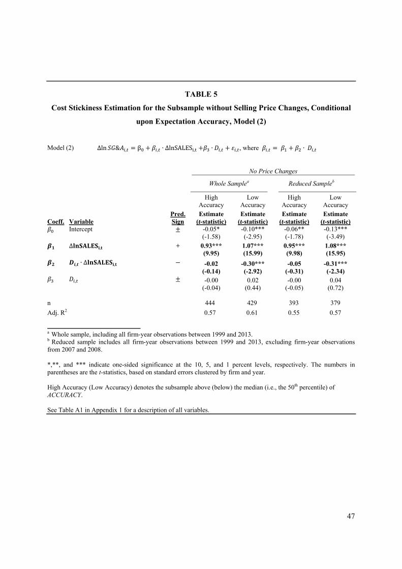
47   

TABLE 5

Cost Stickiness Estimation for the Subsample without Selling Price Changes, Conditional

upon Expectation Accuracy, Model (2)

Model (2) ∆ln & , β , ∙ ∆lnSALES , ∙ , , , where , ∙ ,

No Price Changes

Whole Samplea Reduced Sampleb

High

Accuracy Low

Accuracy High

Accuracy Low

Accuracy

Coeff. Variable Pred. Sign

Estimate (t-statistic)

Estimate (t-statistic)

Estimate (t-statistic)

Estimate (t-statistic)

Intercept -0.05* (-1.58)

-0.10*** (-2.95)

-0.06** (-1.78)

-0.13*** (-3.49)

∆ , + 0.93*** (9.95)

1.07*** (15.99)

0.95*** (9.98)

1.08*** (15.95)

, ∙ ∆ , -0.02 (-0.14)

-0.30*** (-2.92)

-0.05 (-0.31)

-0.31*** (-2.34)

, -0.00 (-0.04)

0.02 (0.44)

-0.00 (-0.05)

0.04 (0.72)

n 444 429 393 379

Adj. R2

0.57 0.61 0.55 0.57

a Whole sample, including all firm-year observations between 1999 and 2013. b Reduced sample includes all firm-year observations between 1999 and 2013, excluding firm-year observations from 2007 and 2008. *,**, and *** indicate one-sided significance at the 10, 5, and 1 percent levels, respectively. The numbers in parentheses are the t-statistics, based on standard errors clustered by firm and year. High Accuracy (Low Accuracy) denotes the subsample above (below) the median (i.e., the 50th percentile) of ACCURACY. See Table A1 in Appendix 1 for a description of all variables.

48   

TABLE 6

The Effect of Demand Volatility on Cost Elasticity, Modeled According to Banker et al. (2014)

Model (3): ∆ln & , β , ∙ ∆lnSALES , ∙ , , ,

where , ∙ _ , ∙ ,

Model (3)

All

Observations Demand Increase

Demand Decrease

Coeff. Variable Pred. Sign

Estimate (t-statistic)

Estimate (t-statistic)

Estimate (t-statistic)

Intercept -0.03*** (-3.59)

-0.02 (-0.74)

-0.14*** (-4.52)

∆ , + 1.08*** (24.09)

1.11*** (14.77)

0.81*** (10.95)

∆ , ∙ _ , -0.23*** (-3.05)

-0.29*** (-2.70)

-0.08 (-0.99)

Controls

∆lnSALES , ∙ , -0.02*** (-5.47)

-0.01 (-0.91)

0.04** (1.79)

, -0.01** (-1.88)

-0.02*** (-2.78)

0.03*** (3.28)

Industry slope and main effect yes yes yes

n 4,105 2,179 1,926

Adj. R2 0.67 0.48 0.37

*,**, and *** indicate one-sided significance at the 10, 5, and 1 percent levels, respectively. The numbers in parentheses are the t-statistics, based on standard errors clustered by firm. The following control variables , are included as both fixed effects as well as interaction effects: GDP growth , and industry classification .

_ , STD ∆lnSALES , See Table A1 in Appendix 1 for a description of all variables.

49   

TABLE 7

The Effect of Demand Volatility on Cost Elasticity Moderated by Accuracy of Expectations

Model (4): ∆ln & , β , ∙ ∆lnSALES , ∙ , ∙ , , ,

where , ∙ _ , ∙ _ , ∙ , ∙

,

Model (4)

All Observations Demand Increase

Demand Decrease

Coeff. Variable Pred. Sign

Estimate (t-statistic)

Estimate (t-statistic)

Estimate (t-statistic)

Intercept -0.03*** (-2.61)

-0.02 (-1.05)

-0.16*** (-4.60)

∆ , + 1.09*** (24.35)

1.12*** (15.25)

0.81*** (11.01)

∆ , ∙ _ , -0.22*** (-2.75)

-0.22** (-1.95)

-0.20** (-2.09)

∆ , ∙ _ ,

∙ , / a -0.06

(-0.76) -0.28** (-2.08)

0.40** (2.33)

, + -0.01 (-0.72)

0.03 (0.73)

0.08** (1.77)

Controls ∆lnSALES , ∙ ,

-0.02*** (-5.49)

-0.01 (-0.89)

0.04** (1.77)

,

-0.01** (-1.87)

-0.02*** (-2.78)

0.03*** (3.21)

Industry slope and main effect yes yes yes

n 4,105 2,179 1,926

50   

Table 7 continued:

Model (4)

All

Observations Demand Increase

Demand Decrease

Adj. R2 0.67 0.48 0.37

a – (+) for demand increase (decrease). *,**, and *** indicate one-sided significance at the 10, 5, and 1 percent levels, respectively. The numbers in parentheses are the t-statistics, based on standard errors clustered by firm. The following control variables , are included as both fixed effects as well as interaction effects: GDP growth , and industry classification .

_ , STD ∆lnSALES ,

. naturallog % 1 with % # /# .

See Table A1 in Appendix 1 for a description of all variables.

51   

FIGURE 1

Resource Adjustment under Uncertainty

 

Adapted from Hamermesh (1993, 224). The figure shows how managers adjust resources differently in response to expected compared to unexpected changes in demand. Specifically, when a drop in demand is expected, managers can prepare to start cutting resources quickly after the demand shock hits. When a drop in demand is unexpected, the adjustment is delayed and less smooth.

Resource adjustment when demand shock is less accurately expected Resource adjustment when demand shock is more accurately expected

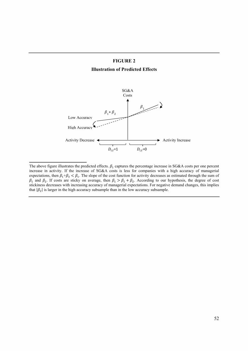
52   

FIGURE 2

Illustration of Predicted Effects

The above figure illustrates the predicted effects. captures the percentage increase in SG&A costs per one percent increase in activity. If the increase of SG&A costs is less for companies with a high accuracy of managerial expectations, then + . The slope of the cost function for activity decreases as estimated through the sum of

and . If costs are sticky on average, then . According to our hypothesis, the degree of cost stickiness decreases with increasing accuracy of managerial expectations. For negative demand changes, this implies that | | is larger in the high accuracy subsample than in the low accuracy subsample.

SG&A Costs

1+  2

1

, =1

Activity Increase Activity Decrease

, =0

Low Accuracy

High Accuracy

53   

FIGURE 3

Case Example for Estimating the Variable _ ,

_ , 1

Expected demand in next three months (reported in t)

Actual demand in previous three months

(reported in t+3)

Case a) Demand Increase Demand Increase

Case b) Demand Decrease Demand Decrease

Case c) No Change in Demand No Change in Demand

_ ,

Expected demand in next three months (reported in t)

Actual demand in previous three months

(reported in t+3)

Case a) Demand Increase Demand Decrease

Case b) Demand Decrease Demand Increase

Case c) No Change in Demand Demand Decrease

Case d) No Change in Demand Demand Increase

Case e) Demand Increase No Change in Demand

Case f) Demand Decrease No Change in Demand

The information on expected demand and actual demand are obtained from the Danish tendency survey conducted as part of the Joint Harmonized EU Program of Business and Consumer Surveys (http://ec.europa.eu/economy_finance/db_indicators/surveys/index_en.htm). The survey question refers to managers’ expectations about demand over the next three months and the actual demand development during the past three months. Therefore, expected demand at t and actual demand in t+3 are compared.

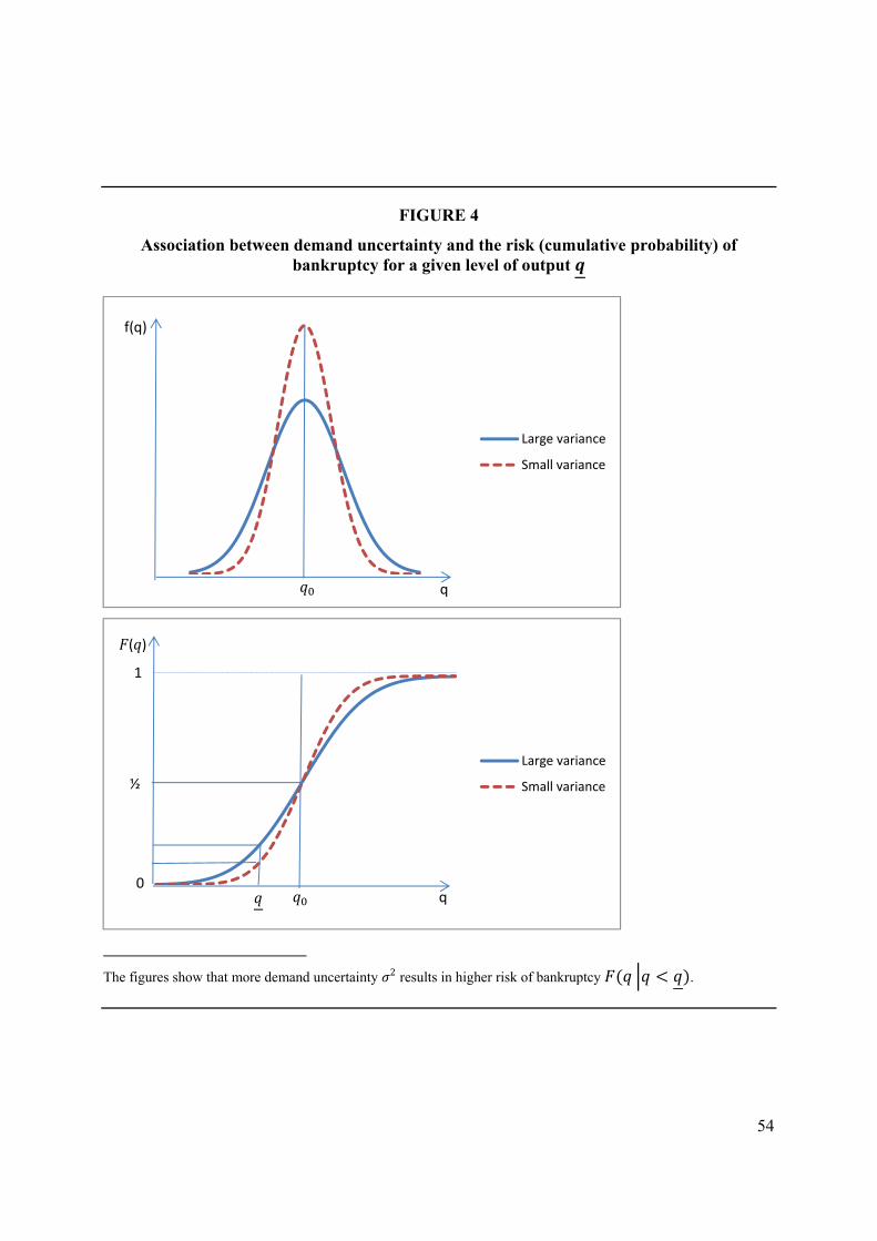
54   

FIGURE 4

Association between demand uncertainty and the risk (cumulative probability) of bankruptcy for a given level of output

The figures show that more demand uncertainty 2 results in higher risk of bankruptcy .

Large variance

Small variance

q

f(q)

Large variance

Small variance

0

( )

1

q

½