Exp and Num Invst of Flow Fields Bhind a WT With Flanged Diffuser

ARTICLE IN PRESS

Journal of Wind Engineering

and Industrial Aerodynamics 93 (2005) 951–970

0167-6105/$ -

doi:10.1016/j

�CorrespoE-mail ad

www.elsevier.com/locate/jweia

Experimental and numerical investigationsof flow fields behind a small wind turbine

with a flanged diffuser

K. Abea,�, M. Nishidab, A. Sakuraia, Y. Ohyac, H. Kiharaa,E. Wadad, K. Satod

aDepartment of Aeronautics and Astronautics, Kyushu University, Hakozaki, Higashi-ku, Fukuoka 812-8581, JapanbDepartment of Aerospace Systems Engineering, Sojo University, Ikeda, Kumamoto 860-0082, Japan

cResearch Institute for Applied Mechanics, Kyushu University, Kasuga-Kouen, Kasuga 816-8580, JapandGraduate student, Department of Aeronautics and Astronautics, Kyushu University, Hakozaki,

Higashi-ku, Fukuoka 812-8581, Japan

Received 5 October 2004; received in revised form 8 September 2005; accepted 19 September 2005

Available online 27 October 2005

Abstract

Experimental and numerical investigations were carried out for flow fields of a small wind turbine

with a flanged diffuser. The present wind-turbine system gave a power coefficient higher than the

Betz limit (¼ 16=27) owing to the effect of the flanged diffuser. To elucidate the flow mechanism,

mean velocity profiles behind a wind turbine were measured using a hot-wire technique. By

processing the obtained data, characteristic values of the flow fields were estimated and compared

with those for a bare wind turbine. In addition, computations corresponding to the experimental

conditions were made to assess the predictive performance of the simulation model presently used

and also to investigate the flow field in more detail. The present experimental and numerical results

gave useful information about the flow mechanism behind a wind turbine with a flanged diffuser. In

particular, a considerable difference was seen in the destruction process of the tip vortex between the

bare wind turbine and the wind turbine with a flanged diffuser.

r 2005 Elsevier Ltd. All rights reserved.

Keywords: Wind turbine; Flanged diffuser; Tip vortex; Separation; CFD; Turbulence; Non-linear Eddy-viscosity

model; Disk-loading method

see front matter r 2005 Elsevier Ltd. All rights reserved.

.jweia.2005.09.003

nding author. Tel.: +81926 423723; fax: +81 926 423752.

dress: [email protected] (K. Abe).

www.elsevier.com/locate/jweia

ARTICLE IN PRESSK. Abe et al. / J. Wind Eng. Ind. Aerodyn. 93 (2005) 951–970952

1. Introduction

The power in wind is well known to be proportional to the cubic power of the windvelocity approaching the wind turbine. This means that even a small amount ofacceleration gives a large increase in the energy output. Therefore, many research groupshave tried to find a way to accelerate the approaching wind effectively [1–7].Recently, Ohya et al. [8,9] have developed an effective wind–acceleration system.

Although it adopts a diffuser-shaped structure surrounding a wind turbine like the otherspreviously proposed, the feature that distinguishes it from the others is a large flangeattached at the exit of diffuser shroud. Fig. 1 illustrates an overview of the presentwind–acceleration system. A flange generates a large separation behind it, where a verylow-pressure region appears to draw more wind compared to a diffuser with no flange.Owing to this effect, the flow coming into the diffuser can be effectively concentrated andaccelerated. In this system, the maximum velocity is obtained near the inlet of diffuser andthus a wind turbine is located there as shown in Fig. 1. Although this wind–turbine system

(a)

(b)

Fig. 1. Schematic view of a diffuser-shrouded wind turbine: (a) overview of system; (b) flow mechanism around a

flanged diffuser.

ARTICLE IN PRESSK. Abe et al. / J. Wind Eng. Ind. Aerodyn. 93 (2005) 951–970 953

has already shown some promising results [8,9], more detailed investigations of flow fieldsinside the diffuser are still needed to achieve the best performance.

Having considered the above background, in this study experimental and numericalinvestigations are carried out for flow fields of a small wind turbine with a flanged diffuser(i.e. a diffuser-shrouded wind turbine). In the experiments, mean velocity profiles behindthe wind turbine are measured using a hot-wire technique. Furthermore, computationscorresponding to the experimental conditions are made to assess the predictiveperformance of the simulation model presently used and also to investigate the flow fieldin more detail. By processing the obtained data, characteristic values of the flow fields areestimated and compared with those for a bare wind turbine.

2. Experimental apparatus

All measurements were performed in a large wind tunnel at the Department ofAeronautics and Astronautics, Kyushu University. It has a measurement section of 2.5m(width) �1:5m (height), with a maximum wind velocity of 20m/s. In this study, a windturbine is located 500mm downstream of the wind-tunnel exit. The wind turbine was athree-bladed rotor with a diameter of 388mm. The blade was designed for the diffuser-shrouded wind turbine currently tested, with the aid of the design theory developed byInoue et al. [10].

Fig. 2 gives detailed information on the diffuser-shrouded wind turbine. The diffuserconsists of a main diffuser, a flange attached at the rear of the diffuser and an inlet shroudattached at the front. As shown in Fig. 2, the diameter of the diffuser throat was 400mm,where the maximum velocity was obtained and thus where the wind turbine was located.The length of the main diffuser was 500mm and the flange height was 200mm. In this

Fig. 2. Detailed information of the present diffuser-shrouded wind turbine.


experiment, the diameter of the center hub was 80mm and hence the hub/throat ratio was0.2. An AC servomotor was installed in the hub to change the rotational velocity of thewind turbine arbitrarily. Also, a torque meter was installed to measure the axial torquegenerated by the wind turbine.Fig. 3 shows the traverse system used in the present experiment. In this study, a

cylindrical coordinate system was adopted, with x, r and y being the streamwise, radial androtational coordinates, respectively. The origin was set at the location of the blades asshown in Fig. 3(b). The velocity fields behind the wind turbine were measured using a hot-wire technique. In this study, a hot-wire X-probe (KANOMAX) was used, each of whichconsists of a tungsten wire 4mm in diameter and 5mm in length. Since an X-probe canprovide only two components of a velocity, we performed measurements for both x–y andx–r components independently to obtain three-dimensional mean velocity fields. As seen inFig. 3(a), in order not to disturb the flow field, the probe was inserted with a supportingbar 500mm in length. Figs. 3(b) and 4 illustrate schematic images of the measurement

Fig. 3. Traverse system: (a) overview of system; (b) detailed information.

ARTICLE IN PRESS

Fig. 4. Schematic image of measurement: (a) bare wind turbine; (b) diffuser-shrouded wind turbine.

K. Abe et al. / J. Wind Eng. Ind. Aerodyn. 93 (2005) 951–970 955

positions. In the experiments, to measure velocity fields just behind the wind turbine, wefirst set the hot wire at x ¼ 48mm (just 10mm behind the root of the blade) and r ¼ 55mm(15mm away from the hub surface). From this position, the probe was traversed in theradial direction and velocity data were obtained in the r–y plane (see Fig. 3(b)). Moreover,to obtain velocity distributions for the whole flow region, the probe was traversed in thestreamwise direction (see Fig. 4).

The free stream velocity (U0) was specified as 11 and 6.8m/s for the bare wind turbineand the diffuser-shrouded wind turbine respectively. The latter condition (6.8m/s for thediffuser-shrouded wind turbine) was chosen so that the approaching wind velocity could besimilar to that in the case of the bare wind turbine. The Reynolds number based on thediameter of the wind turbine and the free stream velocity was about 2:9� 105 for the barewind turbine and 1:8� 105 for the diffuser-shrouded wind turbine. The measurement at agiven position was started by a trigger signal detected when a selected blade passed a laserbeam. The data-sampling rate was set to between 2 and 10 kHz so as to be enough to


resolve in detail the rotational direction. The resolution was less than 1� (i.e. more than 360samples/rotation) in each case. The same procedure was repeated 150–300 times and theobtained data were ensemble-averaged (i.e. phase-averaged) to calculate mean values ateach point.

3. Numerical method and computational conditions

The present flow field is generally expressed by the continuity and the incompressibleReynolds-averaged Navier–Stokes equations as follows:

qUi

qxi

¼ 0, (1)

rUjqUi

qxj

¼ �qP

qxi

þqqxj

rnqUi

qxj

þqUj

qxi

� �� ruiuj

� �þ Fi, (2)

where ð Þ denotes a Reynolds-averaged value. In the equations, r, P, Ui, ui and nrespectively denote the density, mean static pressure, mean velocity, turbulent fluctuationand kinematic viscosity. In Eq. (2), F i is the body-force term imposed for therepresentation of a load.The present computational procedure is almost the same as that used in the previous

report by Abe and Ohya [11], with some modifications in specifying the newly incorporatedload. The grid system and computational conditions are shown in Fig. 5. In this study, theflow was assumed to be an axisymmetric steady flow, with x and r being the streamwiseand radial coordinates respectively. In Fig. 5, L, D, f and h respectively denote the diffuserlength, diffuser diameter at the throat, diffuser opening angle and height of flange used inthe present experiment, i.e., L=D ¼ 1:25, h=D ¼ 0:5 and f ¼ 12�. In Fig. 5(a), thesubscripts 0, 1, 2 and b denote values at the inlet (free stream), in front of the load(approaching), behind the load and at the exit of the diffuser, respectively. Note that thecomputational domain was determined so as not to create any serious problems for theobtained results [11].In this study, the load inside the diffuser was represented by the following general

expression [11]:

F x ¼Ct

D1

2rUxjUxj; F r ¼ 0, (3)

where Ux is the streamwise velocity. In Eq. (3), Ct and D are the loading coefficient and itsstreamwise width imposed, respectively. In this study, Ct was determined by use of a disk-loading method (see for example, [12,13]), as illustrated in Fig. 6. It was found that Ct canbe evaluated in the two-dimensional cylindrical (x–r) coordinate as follows:

Ct ¼ncðCL cos bþ CD sin bÞf1þ ðro=UxÞ

2g

2pr, (4)

where n is the number of blades, o is the angular velocity of the wind turbine, c is the chordlength and b ¼ tan�1ðUx=roÞ. In Eq. (4), CD and CL are, respectively, the drag and liftcoefficients for the relative angle of attack, a ¼ b� g, where g is the angle of blade setting(see Fig. 6). In this study, the profiles of CD and CL were taken from the database [10] fortwo-dimensional blade sections adopted for the wind turbine. They are shown in Fig. 7.

ARTICLE IN PRESS

(a)

(b)

Fig. 5. Grid system and computational conditions: (a) grid system; (b) computational conditions.


On the other hand, from the relation shown in Fig. 6, the torque generated by the bladescan be estimated as follows:

T ¼

Z r0

rh

dT ¼

Z r0

rh

1

2rfU2

x þ ðroÞ2gðCL sin b� CD cos bÞncrdr

¼

Z r0

rh

1

2rU2

xðCL sin b� CD cos bÞf1þ ðro=UxÞ2gncrdr

¼1

2rZ r0

rh

U2xCZ2pr2 dr, ð5Þ

where r0 and rh denote the radius of blade and hub, respectively. Similarly to the discussionon Ct in Eq. (4), CZ is defined as

CZ ¼ncðCL sin b� CD cos bÞf1þ ðro=UxÞ

2g

2pr. (6)

Therefore, the total torque coefficient generated by the blades can be expressed as

Ctrq ¼T

12rU2

0AD¼

112rU2

0AD

Z r0

rh

dT ¼1

AD

Z r0

rh

CZK22pr2 dr, (7)

ARTICLE IN PRESS

Fig. 6. Overview of disk-loading method.

–5 0 5 10–0.5

0

0.5

1

1.5

0

0.02

0.04

0.06

CD

CL

(Symbols: original data)

Angle of attack (deg)

CL

CD

Fig. 7. Drag and lift coefficients for relative angle of attack (a).

K. Abe et al. / J. Wind Eng. Ind. Aerodyn. 93 (2005) 951–970958

where A ¼ pðD=2Þ2 and Kð¼ U2=U0Þ is the acceleration factor. The power coefficient isestimated as follows:

Cw ¼To

12rU3

0A¼

o12rU3

0A

Z r0

rh

dT ¼1

A

Z r0

rh

roUx

� �CZK

32prdr. (8)

Such being the case, it is of interest that the performance of a wind turbine can be virtuallyevaluated with Eqs. (7) and (8), though no swirl effect is incorporated into the calculation.


It will be later shown that this evaluation procedure provides a powerful tool to obtainuseful information of flow fields at low computational cost.

As shown in Fig. 5(b), concerning the inlet boundary condition, a uniform flow (U0) wasspecified. At the outlet boundary, zero-streamwise gradients were prescribed. Concerning thetop boundary, slip conditions were adopted. No-slip conditions were specified at the walls,where the nearest node was properly placed inside the viscous sublayer. The number of gridpoints in this study was 156� 86. The Reynolds number (Re ¼ U0D=n) was set to 20000. It isnoted that the grid dependency and the Reynolds-number dependency of the computationalresults were carefully examined in the previous report [11], where it was shown that the gridresolution used was enough to obtain almost grid-independent solutions and also that therelatively lower Reynolds-number condition did not cause any serious problems ininvestigating fundamental flow characteristics, at least, for this kind of flow cases. This leadsto a practical way to reduce the computational cost (see for detail [11]).

Calculations were performed with the finite-volume procedure STREAM of Lien andLeschziner [14], followed by several improvements and substantially upgraded by Apsleyand Leschziner [15]. This method uses collocated storage on a non-orthogonal grid and allvariables are approximated on cell faces by the UMIST scheme [16], a TVDimplementation of the QUICK scheme. The solution algorithm is SIMPLE, with aRhie–Chow interpolation for pressure. In this study, to predict complex turbulent flowfields with massive flow separation, the non-linear Eddy-viscosity model proposed by Abeet al. [11] was incorporated into the code. This model is based on former models by Abe etal. [17–19], with some modifications for the length-scale equation. Detailed descriptions ofthe model are given in the reference paper [11].

4. Results and discussion

Fig. 8 compares the distributions of torque coefficient (Ctrq) and power coefficient (Cw)between the bare and diffuser-shrouded wind turbines. In the figure, l is a tip speed ratiodefined as

l ¼r0oU0

. (9)

It is found that the shapes of both Cw and Ctrq are similar between the bare and diffuser-shrouded wind turbines. However, the diffuser-shrouded wind turbine returns much higheroutput power compared to the bare wind turbine. The power coefficient obtained from thediffuser-shrouded wind turbine is about four times as high as that from the bare windturbine. The basic performance of such a wind turbine has been discussed by manyresearch groups (see for example, Rauh and Seelert [3]; Hansen et al. [5]; Inoue et al. [10]),from which it has been pointed out that a diffuser-shrouded wind turbine has thepossibility of giving Cw exceeding the Betz limit ð¼ 16=27Þ owing to the effect of thediffuser placed around the wind turbine.

On the other hand, Fig. 9 compares the distributions of torque coefficient (Ctrq2) andpower coefficient (Cw2) normalized by the local mean velocity just behind the turbineblades (U2, see Fig. 5(a)). They are defined as

Ctrq2 ¼T

12rU2

2AD¼

Ctrq

K2; Cw2 ¼

To12rU3

2A¼

Cw

K3. (10)

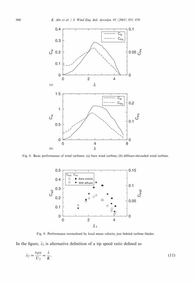
ARTICLE IN PRESS

(a)

(b)

Fig. 8. Basic performance of wind turbines: (a) bare wind turbine; (b) diffuser-shrouded wind turbine.

Fig. 9. Performance normalized by local mean velocity just behind turbine blades.


In the figure, l2 is alternative definition of a tip speed ratio defined as

l2 ¼r0oU2¼

lK. (11)


These values (Ctrq2, Cw2 and l2) are used to investigate the performance of the windturbine under the condition using the local mean velocity just behind the blades. It is ofinterest that both the bare and diffuser-shrouded wind turbines return almost the samepeak performance as seen in Fig. 9, though some discrepancy is seen in the high l2 region.This may indicate that the present wind turbine operates similarly against the approachingwind even with a flanged diffuser. Having considered these facts, it is thought that theaugmentation of the power in the diffuser-shrouded wind turbine is mainly caused by theacceleration of the approaching wind by the flanged diffuser. This is supported by theprevious study of Hansen et al. [5], which evaluated the effect of a diffuser on the poweraugmentation obtained from a wind turbine. Abe and Ohya [11] also investigated theacceleration mechanism of the approaching wind when the flanged diffuser is placedaround a wind turbine.

Fig. 10 gives an overall view of the flow field around the present flanged diffuser atl ¼ 4:5, in the form of the calculated streamfunction plots. As seen in the figure, a flangegenerates a large separation behind it. This is a notable feature of this kind of flow field,which is different from that around a general airfoil-shaped diffuser with no flange. In fact,this separation generates a low-pressure region, owing to which more wind can be drawninto the diffuser [11].

Fig. 11 compares the computational results of Ctrq and Cw with the experimental data. Itis found that the present calculation gives satisfactory predictions for both the bare anddiffuser-shrouded wind turbines. Although some overprediction is seen in higher l regionof the diffuser-shrouded wind turbine, the peak performance is well predicted and thedifference between the bare and diffuser-shrouded wind turbines is sufficiently reproduced.

Fig. 12 shows distributions of the angles in Fig. 6 at l ¼ 2:8 for the bare wind turbine.For this condition, the wind turbine gives high performance and thus no separation isexpected to appear at the blade surface. As seen in the figure, the calculated relative angleof attack (a) is less than 10 degrees at every position, being sufficiently involved in therange shown in Fig. 7. On the other hand, in the low l region, it is easily expected that amay become very large beyond the range in Fig. 7. To investigate flow phenomena indetail, the angular momentum was estimated by the streamwise and rotational velocities.The profiles for two conditions, i.e., l ¼ 2:8 and 1:7 for the bare wind turbine, are

Fig. 10. Streamlines of the flow field (l ¼ 4:5).

ARTICLE IN PRESS

(a)

(b)

Fig. 11. Comparison of basic performance: (a) torque coefficient; (b) power coefficient.

0.2 0.400

20

40

60

80

Inflow angle

Angle of blade setting

Relative angle of attack

r/D

Ang

le (

deg)

Fig. 12. Distributions of inflow angle (b), angle of blade setting (g) and relative angle of attack (a ¼ b� g) atl ¼ 2:8 for the bare wind turbine.


ARTICLE IN PRESS

Fig. 13. Radial distributions of angular momentum for the bare wind turbine.


compared in Fig. 13. It is readily seen that the computational results at l ¼ 2:8 correspondwell to the measured data. This means that the present calculation can provide areasonable distribution in the radial direction as well as a bulk performance for conditionswith no separation at the blade surface.

On the contrary, the measured data in Fig. 11 show that the performance decreases atl ¼ 1:7. As will be shown later, under this condition, separations and their related largevortex-like structures appear on the outer (tip) side. They occupy the region of 1=3 of theblade radius and are highly three-dimensional. Fig. 13 definitely explains that these largeflow structures do not work effectively to generate the angular momentum (i.e. torque).Generally, such complex flow phenomena with large flow structures can never be modeledjust by 2-D database with some simple corrections of 3-D effect, even if 2-D database of anairfoil are available for high angles of attack including two-dimensional massiveseparation. Unfortunately, at least now, there is no data (or model) available to representsuch complex flow phenomena. Such being the case, calculations in the low l region werenot carried out in this study. Although the present results are encouraging from theengineering viewpoint, further investigations will be needed to resolve this issue.

Computational results of the acceleration factor K are compared with those of theexperiment in Fig. 14, where U2 is calculated by averaging the streamwise velocity in thesection just behind the wind turbine (i.e. the load imposed by Eq. (4)). It is seen from thefigure that the present computation returns generally reasonable trends for the variation ofK against l, though the computation gives some underpredictions in the higher l regionespecially for the diffuser-shrouded wind turbine. Fig. 15 compares the calculatedstreamwise-velocity profiles immediately behind the wind turbine with those of theexperiment. The conditions were l ¼ 2:8 (l2 ¼ 3:1) for the bare wind turbine and l ¼ 4:5(l2 ¼ 3:2) for the diffuser-shrouded wind turbine respectively. In the figures, the plots ofthe experimental data have been made by averaging the streamwise velocity in therotational (y) direction. As described earlier, the similar condition of l2 allows us tocompare the results under the condition of similar local mean velocity (i.e. local tip speedratio) just behind the blades. As seen in the figure, a similar trend is seen in the velocityprofiles. The velocity slightly decreases in the region around r=D ¼ 0:4, whereas it increases

ARTICLE IN PRESS

Fig. 14. Comparison of acceleration factor.

0.2 0.4 0.60

0

0.5

1

1.5

2

2.5

Experiment

Calculation

r/D(a)

0.2 0.4 0.600

0.5

1

1.5

2

2.5

Experiment

Calculation

r/D

Ux/

U0

(b)

Ux/

U0

Fig. 15. Comparison of streamwise velocity (x ¼ 48mm): (a) bare wind turbine; (b) diffuser-shrouded wind

turbine.



again at the end of the blade tip (around r=D ¼ 0:5). In particular, in the region close to thediffuser wall (Fig. 15(b)), the flow is greatly accelerated due to the tip clearance. Thepresent computation successfully predicts such a trend of the velocity distribution in the r

direction, though some underprediction is seen especially in Fig. 15(b). Velocity vectors inthe x–r plane are compared in Fig. 16, where vector plots of the experiment have beenmade by averaging the measured velocities in the y direction. It is found that the computedvelocity vectors generally correspond well to those measured in the experiment, thoughsome discrepancy is seen particularly in the downstream region of the bare wind turbine.Fig. 16(b) indicates that the present computation can provide useful information on thedeceleration mechanism inside the diffuser. As seen in the figure, there is no separation on

(a)

(b)

Fig. 16. Comparison of velocity vectors in x–r direction: (a) bare wind turbine; (b) diffuser-shrouded wind

turbine.


the diffuser wall even with a large diffuser opening angle of f ¼ 12�. This notable fact isreasonably predicted by the present computation. From these results, it can be said that thepresent computation sufficiently reproduces fundamental features of the flow fields of thiskind.Such being the case, the present calculation generally returns reasonable results. It is,

however, seen that the approaching wind speed commonly tends to be a littleunderpredicted compared to the measured data. Since this trend is seen even in the casesof the bare wind turbine, it is thought that the main reason may lie in some insufficiency inthe model of the load and/or some influence of ignoring the swirl effect in the calculation.In this respect, further efforts are needed to construct an advanced prediction model,including a new accurate disk-loading model applicable to the low l range. Although therestill remains some margin for improvement, it is said that the present computationalprocedure is very useful for the first assessment of performance in developing new diffuser-shrouded wind turbines.Fig. 17 shows a comparison of the measured velocity vectors just behind the blades for

three representative rotating frequencies, i.e., 2100, 1500 and 900 rpm. It should be notedagain that the present experiment adopts such conditions that local tip speed ratios (l2) canbe similar between the bare and diffuser-shrouded wind turbines at the same rotationalfrequency. As seen in Fig. 9, the conditions of 2100 rpm (l2�4) and 1500 rpm (l2�3) are inthe region of a higher tip speed ratio, where the flow is thought to be smooth with nomassive separation on the blades. On the other hand, 900 rpm (l2�2) is in the region of alower tip speed ratio and then the results give us information of the flow structure in thestall condition. In the cases of 2100 and 1500 rpm, the flow successfully rotates in the ydirection, which means that the blades effectively generate torque. In the region close tothe blade tip, some vortex structures are seen, which are thought to be the tip vortices. It isof interest that similar patterns can be seen for both the bare and diffuser-shrouded windturbines, though the tip vortex of the diffuser-shrouded wind turbine looks stronger thanthat of the bare wind turbine. On the other hand, in the case of 900 rpm, very large flowstructures are clearly seen. These structures occupy the region of 1=4–1=3 of the bladeradius from the blade tip. This kind of large structure is usually thought to be caused bymassive separations occurring at the blade surfaces. They prevent the blades fromgenerating torque as described in Fig. 13 and thus the performance of the wind turbinedecreases as shown in Figs. 8 and 9. From these figures, it is generally said that the flowstructures of the bare and diffuser-shrouded wind turbines are basically similar to eachother, at least, at the location just behind the turbine blades. This corresponds well to theresults of the performance normalized by the local mean velocity (U2) shown in Fig. 9. Inthe region close to the blade tip, however, some discrepancies are seen mainly due to theeffect of the diffuser wall (i.e. the tip clearance).To compare the flow structures of the bare and diffuser-shrouded wind turbines in the

region downstream of the blades, Fig. 18 shows the experimental data of velocity vectorsand streamwise vorticity distributions at three locations in the streamwise direction, i.e.,x ¼ 48mm (x=D ¼ 0:12), 148mm (0.37) and 248mm (0.52). As mentioned above, it isfound again that the flow structures of the diffuser-shrouded wind turbine just behind theturbine blades are generally similar to those of the bare wind turbine except for the regionclose to the blade tip. On the other hand, it is of great interest that completely differenttrends are seen in the downstream region. In particular, rapid destruction of the vortexstructure is seen in the diffuser-shrouded wind turbine, while similar vortex structures

ARTICLE IN PRESS

0.5

0

-0.5

0.50-0.5

2100rpm (λ = 6.3, λ2 = 3.9)2100rpm (λ = 3.6, λ2 = 3.8)

1500rpm (λ = 2.8, λ2 = 3.1)

900rpm (λ = 1.7, λ2 = 1.8) 900rpm (λ = 2.7, λ2 = 2.1)

1500rpm (λ = 4.5, λ2 = 3.3)

5 [m/s]

0.5

0

-0.5

0.50-0.5

5 [m/s]

0.5

0

-0.5

0.50-0.5

5 [m/s]

0.5

0

-0.5

0.50-0.5

5 [m/s]

0.5

0

-0.5

0.50-0.5

5 [m/s]

0.5

0

-0.5

0.50-0.5

5 [m/s]

(a) (b)

Fig. 17. Comparison of velocity vectors behind turbine blades (x ¼ 48mm): (a) bare wind turbine; (b) diffuser-

shrouded wind turbine.


ARTICLE IN PRESS

0.5

0

-0.5

0.50-0.5

x=48mm (x / D = 0.12) x=48mm (x / D = 0.12)

5 [m/s]

0.5

0

-0.5

0.50-0.5

5 [m/s]

0.5

0

-0.5

0.50-0.5

5 [m/s]

0.5

0

-0.5

0.50-0.5

5 [m/s]

0.5

0

-0.5

0.50-0.5

5 [m/s]

0.5

0

-0.5

0.50-0.5

5 [m/s]

(a) (b)

x=148mm (x / D = 0.37) x=148mm (x / D = 0.37)

x=248mm (x / D = 0.52) x=248mm (x / D = 0.52)

vorticity

201612840-4-8-12-16-20 [1/s]

vorticity

201612840-4-8-12-16-20 [1/s]

vorticity

201612840-4-8-12-16-20 [1/s]

vorticity

201612840-4-8-12-16-20 [1/s]

vorticity

201612840-4-8-12-16-20 [1/s]

vorticity

201612840-4-8-12-16-20 [1/s]

Fig. 18. Comparison of velocity vectors and vorticity distributions in r–y planes at 1500 rpm: (a) bare wind

turbine (l ¼ 2:8; l2 ¼ 3:1); (b) diffuser-shrouded wind turbine (l ¼ 4:5; l2 ¼ 3:3).



clearly remain even in the far downstream region of the bare wind turbine (see Fig. 18,x=D ¼ 0:52). This is also supported by the variation of the streamwise vorticity at the threelocations.

5. Concluding remarks

Experimental and numerical investigations were carried out for flow fields of a smallwind turbine with a flanged diffuser (i.e. a diffuser-shrouded wind turbine). By processingthe data obtained, characteristic values of the flow fields were estimated and comparedwith those for a bare wind turbine. The main conclusions derived from the study are asfollows:

�
The present diffuser-shrouded wind turbine provided much a higher power outputcompared to the bare wind turbine. The power coefficient of the diffuser-shrouded windturbine was about four times as high as that of the bare wind turbine. However, whenthe performance was normalized by the local mean velocity just behind the turbineblades, both the bare and diffuser-shrouded wind turbines returned almost the samepeak performance. This may indicate that the wind turbine operates similarly againstthe approaching wind even with a flanged diffuser. It is also thought that the poweraugmentation of this kind of wind turbine is mainly caused by the acceleration of theapproaching wind by a flanged diffuser. � The present computational results generally showed reasonable agreement with the
corresponding experimental data in the range from moderate to high l, where noseparation at the blade surface was expected. On the other hand, in the low l range, thepresent experiment elucidated that very large vortex-like structures were generated.These structures occupied the region of 1=4–1=3 of the blade radius from the blade tip.This may indicate that further efforts are needed to construct a new disk-loading modelrepresenting such complex flow phenomena in the low l range. Although there stillremains some margin for improvement, it is said that the present computationalprocedure is very useful for the first assessment of performance in developing newdiffuser-shrouded wind turbines.
� Flow structures of the diffuser-shrouded wind turbine just behind the blades were
generally similar to those of the bare wind turbine, though some discrepancy was seen inthe region close to the blade tip. On the other hand, completely different trends wereseen in the region downstream of the wind turbine. In particular, it is worth noting thatrapid destruction of the vortex structure was seen in the diffuser-shrouded wind turbine,while similar vortex structures were clearly seen even in the far downstream region ofthe bare wind turbine. This is thought to be a notable feature of this kind of diffuser-shrouded wind turbine.

Acknowledgements

This research was partially supported by the Ministry of Education, Culture, Sports,Science and Technology, Japan (Grant-in-Aids for Scientific Research, No. 14205139, No.15360450), the Ministry of Economy, Trade and Industry (Matching Fund), SumitomoFund (Environment Protection Research), Harada Memorial Fund (Fluid MachineryResearch) and Kyushu University (Program and Project for Education and Research). The


authors wish to express their appreciation to Mr. M. Matsubara of Kyushu University,Fukuoka, Japan for his technical help in the experiments. KA also wishes to express hisappreciation to Professor M.A. Leschziner of Imperial College of Science, Technology andMedicine, London, UK for the support in using the STREAM code.

References

[1] O. Igra, Research and development for shrouded wind turbines, Energy Conversion Manage. 21 (1981)

13–48.

[2] B.L. Gilbert, K.M. Foreman, Experiments with a diffuser-augmented model wind turbine, Trans. ASME,

J. Energy Res. Technol. 105 (1983) 46–53.

[3] A. Rauh, W. Seelert, The Betz optimum efficiency for windmills, Appl. Energy 17 (1984) 15–23.

[4] D.G. Phillips, P.J. Richards, R.G.J. Flay, CFD modelling and the development of the diffuser augmented

wind turbine, Proceedings of the Comp. Wind Eng. 2000, Birmingham, 2000, pp. 189–192.

[5] M.O.L. Hansen, N.N. Sorensen, R.G.J. Flay, Effect of placing a diffuser around a wind turbine, Wind

Energy 3 (2000) 207–213.

[6] M. Nagai, K. Irabu, Momentum theory for diffuser augmented wind turbine, Trans. JSME 53-489 (1987)

1543–1547 (in Japanese).

[7] I. Ushiyama, Introduction of Wind Turbine, Sanseido Press, Tokyo, 1997, pp. 77–84 (in Japanese).

[8] Y. Ohya, T. Karasudani, A. Sakurai, Development of high-performance wind turbine with brimmed diffuser,

J. Japan Soc. Aeronaut. Space Sci. 50 (2002) 477–482 (in Japanese).

[9] Y. Ohya, T. Karasudani, A. Sakurai, M. Inoue, Development of high-performance wind turbine with a

brimmed-diffuser: Part 2, J. Japan Soc. Aeronaut. Space Sci. 52 (2004) 210–213 (in Japanese).

[10] M. Inoue, A. Sakurai, Y. Ohya, A simple theory of wind turbine with a brimmed diffuser, Turbomachinery

30 (2002) 497–502 (in Japanese).

[11] K. Abe, Y. Ohya, An investigation of flow fields around flanged diffusers using CFD, J. Wind Eng. Indust.

Aerodyn. 92 (2004) 315–330.

[12] J.N. Sorensen, C.W. Kock, A model for unsteady rotor aerodynamics, J. Wind Eng. Indust. Aerodyn. 58

(1995) 259–275.

[13] H. Kume, Y. Ohya, T. Karasudani, K. Watanabe, Design of a shrouded wind turbine with brimmed diffuser

using CFD, Proceedings of the Annual Conference of JSAS, The West Side Division, 2003, pp. 51–54 (in

Japanese).

[14] F.S. Lien, M.A. Leschziner, A general non-orthogonal collocated finite volume algorithm for turbulent flow

at all speeds incorporating second-moment turbulence-transport closure, Part 1: Computational

implementation, Comput. Methods Appl. Mech. Eng. 114 (1994) 123–148.

[15] D.D. Apsley, M.A. Leschziner, Advanced turbulence modelling of separated flow in a diffuser, Flow, Turbul.

Combust. 63 (1999) 81–112.

[16] F.S. Lien, M.A. Leschziner, Upstream monotonic interpolation for scalar transport with application to

complex turbulent flows, Int. J. Numer. Methods Fluids 19 (1994) 527–548.

[17] K. Abe, Y.J. Jang, M.A. Leschziner, An investigation of wall-anisotropy expressions and length-scale

equations for non-linear Eddy-viscosity models, Int. J. Heat Fluid Flow 24 (2003) 181–198.

[18] K. Abe, T. Kondoh, Y. Nagano, On Reynolds stress expressions and near-wall scaling parameters for

predicting wall and homogeneous turbulent shear flows, Int. J. Heat Fluid Flow 18 (1997) 266–282.

[19] K. Abe, T. Kondoh, Y. Nagano, A new turbulence model for predicting fluid flow and heat transfer in

separating and reattaching flows—I. Flow field calculations, Int. J. Heat Mass Transfer 37 (1994) 139–151.

Documents

Exp and Num Invst of Flow Fields Bhind a WT With Flanged Diffuser