Chaos, Solitons & Fractals 43 (2010) 25–30

Contents lists available at ScienceDirect

Chaos, Solitons & FractalsNonlinear Science, and Nonequilibrium and Complex Phenomena

journal homepage: www.elsevier .com/locate /chaos

Existence and uniqueness of limit cycles in a class of second orderODE’s with inseparable mixed terms q

M. Sabatini ⇑Dip. di Matematica, Univ. di Trento, I-38050 Povo, TN, Italy

a r t i c l e i n f o

Article history:Received 16 April 2010Accepted 19 July 2010

0960-0779/$ - see front matter � 2010 Elsevier Ltddoi:10.1016/j.chaos.2010.07.002

q A previous version of this paper can be foundarXiv:1003.0803v1 [math.DS].⇑ Tel.: +39 0461 881670; fax: +39 0461 881624.

E-mail address: marco.sabatini@unitn.it

a b s t r a c t

We prove a uniqueness result for limit cycles of the second order ODE€xþ _x/ðx; _xÞ þ gðxÞ ¼ 0. Under mild additional conditions, we show that such a limit cycleattracts every non-constant solution. As a special case, we prove limit cycle’s uniquenessfor an ODE studied in [5] as a model of pedestrians’ walk. This paper is an extension toequations with a non-linear g(x) of the results presented in [8].

� 2010 Elsevier Ltd. All rights reserved.

1. Introduction

The simplest non-linear continuous dynamical systemsoriginate from the study of planar differential systems,

_x ¼ Pðx; yÞ; _y ¼ Qðx; yÞ; ðP;QÞ 2 C1ðR2;R2Þ: ð1Þ

Special cases of such systems are Lotka–Volterra ones, andsystems equivalent to Liénard equations,

_x ¼ y� FðxÞ; _y ¼ �gðxÞ; ð2Þ

or to Rayleigh equations

_x ¼ y; _y ¼ �gðxÞ � f ðyÞ: ð3Þ

All of them arise as mathematical models of biological,physical, engineering systems [3]. The study of the dynam-ics of (1) strongly depends on the existence and stabilityproperties of special solutions such as equilibrium pointsand non-constant isolated periodic solutions. In particular,if an attracting non-constant periodic solution exists, thenit dominates the dynamics of (1) in an open, connectedsubset of the plane, its region of attraction. Studying thenumber and location of isolated periodic solutions, usuallycalled limit cycles, is by no means a trivial question, asshown by the resistance of Hilbert XVI problem (see [10],

. All rights reserved.

at www.arxiv.org as

problem 13). In some cases such a region of attractioncan even extend to cover the whole plane, with the uniqueexception of an equilibrium point. In such a case the limitcycle is unique and dominates the system’s dynamics, as in[4]. Uniqueness theorems for limit cycles have been exten-sively studied (see [2,14,15], for recent results and exten-sive bibliographies). Limit cycle’s uniqueness is a relevantfeature even in discrete time systems, which are often re-lated to continuous time systems [11]. Sometimes, suitablesymmetry conditions have been used, in order to simplifythe study of such systems. In particular Z2 symmetry, thatis orbital symmetry with respect to one axis, has proved tobe useful in approaching similar problems [13].

Most of the results obtained for continuous timedynamical systems in the plane are concerned with theclassical Liénard system (2) and its generalizations, such as

_x ¼ nðxÞ½uðyÞ � FðxÞ�; _y ¼ �fðyÞgðxÞ: ð4Þ

Such a class of systems also contain Lotka–Volterra sys-tems and systems equivalent to Rayleigh Eq. (3) as specialcases.

Even if the systems (4) reach a high level of generality,compared to Van der Pol system,

_x ¼ y� � x3

3� x

� �; _y ¼ �x;

the first one to be investigated in relation to existence anduniqueness of limit cycles, an evident limitation is given bythe fact that the variables x and y appear separately, so that

26 M. Sabatini / Chaos, Solitons & Fractals 43 (2010) 25–30

mixed terms are products of single-variable functions.Since models displaying a different combination of vari-ables do exist, different methods are desirable, in particu-lar in absence of symmetry conditions.

A recent result [2] is concerned with systems equivalentto

€xþXN

k¼0

f2kþ1ðxÞ _x2kþ1 þ x ¼ 0; ð5Þ

with f2k+1(x) increasing for x > 0, decreasing for x < 0,k = 0, . . . ,N. On the other hand, there exist classes of secondorder models which are not covered by previous results.This is the case of a model developed in [5] to describethe pedestrian’s walk, which leads to the equation

€xþ � _xðx2 þ x _xþ _x2 � 1Þ þ x ¼ 0; � > 0: ð6Þ

Such an equation can be considered as a special case of amore general class of equations

€xþ _x/ðx; _xÞ þ gðxÞ ¼ 0: ð7Þ

In this paper we study the class (7), assuming /ðx; _xÞ tohave strictly star-shaped level sets and xg(x) > 0 for x – 0.We prove a uniqueness result for limit cycles, and, undersuitable additional assumptions, we show that a limit cycleexists and attracts every non-constant solution. Since� _xðx2 þ x _xþ _x2 � 1Þ has strictly star-shaped level sets, themodel introduced in [5] has a unique limit cycle, attractingevery non-constant solution. We also prove that the un-ique limit cycle c is hyperbolic, i.e. that

RdivðcðtÞÞdt – 0,

where div is the divergence of the vector field. Hyperbolic-ity, which is not a consequence of attractivity, plays a mainrole in perturbation problems [7].

The result we present here is as well applicable to sev-eral equations of Liénard and Rayleigh type, in particularwhen they have a non-linear g(x).

This paper is organized as follows: In Section 2 we studythe Eq. (7), assuming g(x) to be linear. We first prove theuniqueness theorem. The main tools applied here is auniqueness result proved in [6]. Then we introduce somemild additional hypotheses on the sign of /ðx; _xÞ, underwhich the unique limit cycle attracts every non-constantsolution. Then, in Section 3, we assume g(x) to be non-lin-ear. We reduce the study of such a case to that of the linearg(x), by means of Conti–Filippov transformation [9]. Thestructure of Section 3 is very similar to that of Section 2,the main difference being the derivation of the conditionon /ðx; _xÞ which implies the strict star-shapedness prop-erty for the transformed system.

2. Linear g(x)

Let X � R2 be a star-shaped set. We denote partialderivatives by subscripts, i.e. /x is the derivative of / w.r.to x, etc. We say that a function / 2 C1(X; R) is star-shapedif (x,y) � r/ = x/x + y/y does not change sign. We say that /is strictly star-shaped if (x,y) � r/ – 0, except at the originO = (0,0). We say that c(t) is positively bounded if thesemi-orbit c+ = {c(t), t P 0} is contained in a bounded set.Similarly for the negative boundedness. We say that an or-bit is an open unbounded orbit if it is both positively and

negatively unbounded. We say that a set X is invariant ifevery orbit starting at a point of X is entirely contained inX. For other definitions related to dynamical systems, werefer to [1]. We call ray a half straight line having originat the point (0,0).

In this section we are concerned with the equation

€xþ _x/ðx; _xÞ þ kx ¼ 0; k 2 R; k > 0; ð8Þ

where / 2 C1ðX; RÞ, X star-shaped subset of R2. Withoutloss of generality, possibly performing a time rescaling,we may restrict to the case k = 1. Let us consider a systemequivalent to the Eq. (8), for k = 1,

_x ¼ y _y ¼ �x� y/ðx; yÞ: ð9Þ

We denote by c(t,x*,y*) the unique solution of the system(9) such that c(0,x*,y*) = (x*,y*). We first consider a suffi-cient condition for limit cycle’s uniqueness. We set

Aðx; yÞ ¼ y _x� x _y ¼ y2 þ x2 þ xy/ðx; yÞ:

The sign of A(x,y) is opposite to that of the angular speed ofthe solutions of (9). Our uniqueness result comes fromTheorem 2 of [6], in the form of Corollary 6.

Theorem 1. Let / 2 ðR2; RÞ be a strictly star-shaped func-tion. Then (9) has at most one limit cycle, which is hyperbolic.

Proof. Without loss of generality, one may assume that,for (x,y) – (0,0), x/x + y/y > 0. The proof can be performedanalogously for the opposite inequality.

We claim that rA(x,y) does not vanish on the setA0 = {(x,y) : A(x,y) = 0}n{(0,0)}. In fact, rA and A vanishsimultaneously at (x,y) if and only if

2xþ y/þ xy/x ¼ 0;2yþ x/þ xy/y ¼ 0;

x2 þ y2 þ xy/ ¼ 0:

8><>: ð10Þ

Multiplying the first equation by x, the second one by y andre-ordering terms yields

xy/ ¼ �x2ð2þ y/xÞ;xy/ ¼ �y2ð2þ x/yÞ;xy/ ¼ �x2 � y2:

8><>:Multiplying the third equation by �2 and summing it withthe first two equations yields

xyðx/x þ y/yÞ ¼ 0:

Since, by hypothesis, x/x + y/y – 0 except at O, one hasxy = 0. If x = 0, then by the third equation in (10) one hasy = 0. Similarly, if y = 0.

This shows that, at every point, A0 is locally a graph.Additionally, every ray {(tcosh, tsinh), t > 0}, meets A0 atmost at a point. In fact, for xy – 0, one has

Aðt cos h; t sin hÞ ¼ 0 () /ðt cos h; t sin hÞ ¼ 1cos h sin h

:

The condition x/x + y/y > 0 implies that / is an increasingfunction of t on every ray. Hence on every ray not con-tained in an axis there exists at most one t such that

M. Sabatini / Chaos, Solitons & Fractals 43 (2010) 25–30 27

/ðt cos h; t sin hÞ ¼ 1cos h sin h. As for xy = 0, A vanishes only at

O.Moreover, working as above, one can show that A0 does

not meet the axes.The radial derivative Ar of A is given by

Ar ¼xAx þ yAy

r¼ 1

rð2Aþ xyðx/x þ y/yÞÞ: ð11Þ

Let (x*,y*) be a point of the first orthant, i.e.x* > 0, y* > 0. IfA(x*,y*) P 0, then Ar > 0 at (x*,y*) and at every point(rx*,ry*) with r > 1, hence A is strictly increasing on the halfstraight line {(rx*,ry*) : r > 1}. Now, let (x*,y*) be a point ofthe second orthant, i.e. x* > 0, y* < 0. If A(x*,y*) < 0, thenAr < 0 at (x*,y*) and at every point (rx*,ry*) with r > 1, henceA is strictly decreasing on the half straight line {(rx*,ry*) :r > 1}. The same argument allows to prove that in the thirdorthant A behaves as in the first one, and in the fourth orth-ant A behaves as in the second one.

Assume, by absurd, two distinct limit cycles to exist.The system (9) has a unique critical point, hence they areconcentric. Let l1 be the inner one, l2 be the external one.Let D be the annular region bounded by l1 and l2. Weclaim that A(x,y) > 0 in D. We prove it by proving that, forevery orbit c contained in D, A(c(t)) > 0. Let us observe thatevery orbit in D has to meet every semi-axis, otherwise itspositive limit set would contain a critical point differentfrom O. On every semi-axis one has A(x,y) > 0. Assume first,by absurd, A(c(t)) to change sign. Then there exist t1 < t2

such that A(c(t1)) > 0, A(c(t2)) < 0, and and c(ti), i = 1, 2 areon the same ray. Assume c(ti), i = 1, 2 to be in the firstorthant. Two cases can occur: either jc(t1)j < jc(t2)j orjc(t1)j > jc(t2)j. The former, jc(t1)j < jc(t2)j, contradicts thefact that A is radially increasing in the first orthant, henceone has jc(t1)j > jc(t2)j. The orbit c(t1) crosses the segmentR = {rc(t1), 0 < r < 1}, going towards the positive y-semi-axis. Let G be the region bounded by the positive y-semi-axis, the ray {r c(t1), r > 0} and the portions of l1, l2

meeting the y-axis and such a ray. The orbit c cannotremain in G, since in that case G would contain a criticalpoint different from O. Also, c cannot leave G crossing thepositive y-semi-axis, because A(x,y) > 0 on such an axis.Hence c leaves G passing again through the segment R.That implies the existence of t3 > t2, such that c(t3) lies onthe ray {rc(t1), 0 < r}. Again, one cannot have jc(t3)j < jc(t2)j,since A(c(t3)) > 0 implies A increasing on the half straightline rc(t3)), r > 1, hence one has jc(t3)j > jc(t2)j. Also, onecannot have jc(t3)j < jc(t1)j, otherwise c would enter apositively invariant region, bounded by the curve c(t), fort1 6 t 6 t3, and by the segment with extrema c(t1), c(t3),hence there would exist a critical point different from O. Asa consequence, one has jc(t3)j > jc(t1)j. Since A(x,y) > 0 onthe segment joining c(t1) and c(t3), such a segment, withthe portion of orbit joining c(t1) and c(t3) bounds a regionwhich is negatively invariant for (9), hence contains acritical point different from O, contradiction.

This argument may be adapted to treat also the case of aray in the second orthant, replacing the positive y-semi-axis with the positive x-semi-axis, and reversing therelative positions of the points c(t1), c(t2), c(t3). In theother orthants one repeats the arguments of the first andsecond orthants, respectively.

Finally, assume that A(c(t)) = 0 at some point (x*,y*). If(x*,y*) is interior to D, then on the ray {(rx*,ry*), r > 0},there exist points interior to D with A(rx*,ry*) < 0. Then wecan apply the above argument to the orbits starting at suchpoints. If (x*,y*) belongs to the boundary of D, then it is onl1 or on l2. Assume (x*,y*) = l1(t*), for some t* (theargument works similarly on l2). Since A(l1(t*)) = 0,l1 istangent to the ray {(rx*,ry*), r > 0}. On the other hand,Ar ¼

xyðx/xþy/yÞr – 0 at (x*,y*), hence A0 is neither tangent to

the ray {(rx*,ry*), r > 0}, nor to l1 at l1(t*). This implies thatA0 and l1 are transversal at (x*,y*), so that a portion of A0

enters D. Since A0 separates points where A > 0 from pointswhere A < 0, also in this case there exist points interior to Dwith A < 0.

Now we can restrict to the annular region D and applycorollary 6 in [6]. In order to apply such a corollary, one hasto compute the expression

m ¼PðxQ x þ yQ yÞ � QðxPx þ yPyÞ

yP � xQ;

where P and Q are the components of the considered vectorfield. For system (9), one has

mA ¼ yð�x� xy/x � y/� y2/yÞ � ð�x� y/Þy¼ �y2 x/x þ y/y

� �6 0:

The function m vanishes only for y = 0. For both cycles onehasZ Ti

0mðliðtÞÞdt < 0; i ¼ 1;2;

where Ti is the period of li, i = 1, 2. Hence both cycles, byTheorem 1 in [6], are attractive. Let A1 be the region ofattraction of l1. A1 is bounded, because it is enclosed byl2, which is not attracted to l1. The external componentof A1’s boundary is itself a cycle l3, because (9) has justone critical point at O. Again,Z T3

0mðl3ðtÞÞdt < 0;

hence l3 is attractive, too. This contradicts the fact that thesolutions of (9) starting from its inner side are attracted tol1. Hence the system (9) can have at most a single limit cy-cle l(t).

Finally, since, as proved in [6], for a T-periodic cyclecycle l(t) one has

Z T

0divðlðtÞÞdt ¼

Z T

0mðlðtÞÞdt;

such a cycle is hyperbolic. h

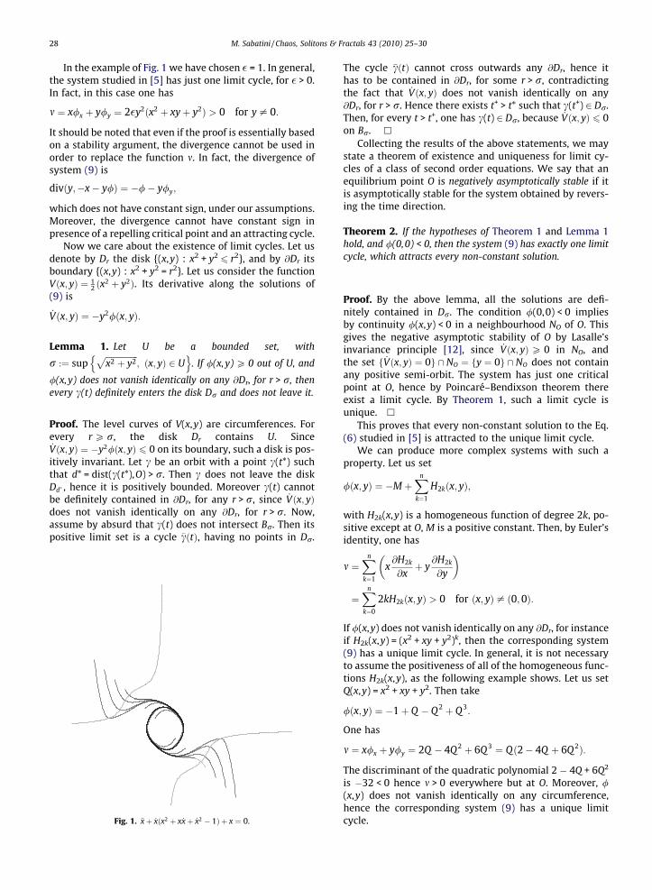
The angular velocity of the solutions need not be nega-tive at every point of the plane. In fact, even a simple sys-tem as that one studied in (6) has negative angular velocityonly in a proper subset of the plane. In Fig. 1 we have plot-ted in black some orbits of the Eq. (6) tending at the limitcycle, together with, in grey, the two components of thecurve A0. The orbits cross A0 at the points where theirangular velocity changes sign. The picture has been pro-duced by using the package DEtools of the computer sys-tem Maple 11.

28 M. Sabatini / Chaos, Solitons & Fractals 43 (2010) 25–30

In the example of Fig. 1 we have chosen � = 1. In general,the system studied in [5] has just one limit cycle, for � > 0.In fact, in this case one has

m ¼ x/x þ y/y ¼ 2�y2ðx2 þ xyþ y2Þ > 0 for y – 0:

It should be noted that even if the proof is essentially basedon a stability argument, the divergence cannot be used inorder to replace the function m. In fact, the divergence ofsystem (9) is

divðy;�x� y/Þ ¼ �/� y/y;

which does not have constant sign, under our assumptions.Moreover, the divergence cannot have constant sign inpresence of a repelling critical point and an attracting cycle.

Now we care about the existence of limit cycles. Let usdenote by Dr the disk {(x,y) : x2 + y2

6 r2}, and by @Dr itsboundary {(x,y) : x2 + y2 = r2}. Let us consider the functionVðx; yÞ ¼ 1

2 ðx2 þ y2Þ. Its derivative along the solutions of(9) is

_Vðx; yÞ ¼ �y2/ðx; yÞ:

Lemma 1. Let U be a bounded set, with

r :¼ supffiffiffiffiffiffiffiffiffiffiffiffiffiffiffiffix2 þ y2

p; ðx; yÞ 2 U

n o. If /(x,y) P 0 out of U, and

/(x,y) does not vanish identically on any @Dr, for r > r, thenevery c(t) definitely enters the disk Dr and does not leave it.

Proof. The level curves of V(x,y) are circumferences. Forevery r P r, the disk Dr contains U. Since_Vðx; yÞ ¼ �y2/ðx; yÞ 6 0 on its boundary, such a disk is pos-itively invariant. Let c be an orbit with a point c(t*) suchthat d* = dist(c(t*),O) > r. Then c does not leave the diskDd� , hence it is positively bounded. Moreover c(t) cannotbe definitely contained in @Dr, for any r > r, since _Vðx; yÞdoes not vanish identically on any @Dr, for r > r. Now,assume by absurd that c(t) does not intersect Br. Then itspositive limit set is a cycle �cðtÞ, having no points in Dr.

Fig. 1. €xþ _xðx2 þ x _xþ _x2 � 1Þ þ x ¼ 0.

The cycle �cðtÞ cannot cross outwards any @Dr, hence ithas to be contained in @Dr, for some r > r, contradictingthe fact that _Vðx; yÞ does not vanish identically on any@Dr, for r > r. Hence there exists t+ > t* such that c(t+) 2 Dr.Then, for every t > t+, one has c(t) 2 Dr, because _Vðx; yÞ 6 0on Br. h

Collecting the results of the above statements, we maystate a theorem of existence and uniqueness for limit cy-cles of a class of second order equations. We say that anequilibrium point O is negatively asymptotically stable if itis asymptotically stable for the system obtained by revers-ing the time direction.

Theorem 2. If the hypotheses of Theorem 1 and Lemma 1hold, and /(0,0) < 0, then the system (9) has exactly one limitcycle, which attracts every non-constant solution.

Proof. By the above lemma, all the solutions are defi-nitely contained in Dr. The condition /(0,0) < 0 impliesby continuity /(x,y) < 0 in a neighbourhood NO of O. Thisgives the negative asymptotic stability of O by Lasalle’sinvariance principle [12], since _Vðx; yÞP 0 in NO, andthe set f _Vðx; yÞ ¼ 0g \ NO ¼ fy ¼ 0g \ NO does not containany positive semi-orbit. The system has just one criticalpoint at O, hence by Poincaré–Bendixson theorem thereexist a limit cycle. By Theorem 1, such a limit cycle isunique. h

This proves that every non-constant solution to the Eq.(6) studied in [5] is attracted to the unique limit cycle.

We can produce more complex systems with such aproperty. Let us set

/ðx; yÞ ¼ �M þXn

k¼1

H2kðx; yÞ;

with H2k(x,y) is a homogeneous function of degree 2k, po-sitive except at O, M is a positive constant. Then, by Euler’sidentity, one has

m ¼Xn

k¼1

x@H2k

@xþ y

@H2k

@y

� �

¼Xn

k¼0

2kH2kðx; yÞ > 0 for ðx; yÞ – ð0;0Þ:

If /(x,y) does not vanish identically on any @Dr, for instanceif H2k(x,y) = (x2 + xy + y2)k, then the corresponding system(9) has a unique limit cycle. In general, it is not necessaryto assume the positiveness of all of the homogeneous func-tions H2k(x,y), as the following example shows. Let us setQ(x,y) = x2 + xy + y2. Then take

/ðx; yÞ ¼ �1þ Q � Q 2 þ Q 3:

One has

m ¼ x/x þ y/y ¼ 2Q � 4Q2 þ 6Q 3 ¼ Qð2� 4Q þ 6Q 2Þ:

The discriminant of the quadratic polynomial 2 � 4Q + 6Q2

is �32 < 0 hence m > 0 everywhere but at O. Moreover, /(x,y) does not vanish identically on any circumference,hence the corresponding system (9) has a unique limitcycle.

M. Sabatini / Chaos, Solitons & Fractals 43 (2010) 25–30 29

3. Non-linear g(x)

Even if the equation we consider in this section are of amore general type, we actually derive our result from thatof the previous section, so that we can consider what fol-lows a corollary of the previous result. Let us considerthe equation

€xþ _x/ðx; _xÞ þ gðxÞ ¼ 0: ð12Þ

We assume that xg(x) > 0 for x – 0, g 2 C1(R; R), g0(0) – 0.As a consequence, g(0) = 0, and x(t) � 0 is the unique con-stant solution of (12). We could consider equations definedin smaller subset of the plane, without essential changes.The main tools is the so-called Conti–Filippov transforma-tion, which acts on the equivalent system

_x ¼ y; _y ¼ �gðxÞ � y/ðx; yÞ; ð13Þ

in such a way to take the conservative part of the vectorfield into a linear one. Let us set GðxÞ ¼

R x0 gðsÞds, and de-

note by r(x) the sign function, whose value is �1 forx < 0, 0 at 0, 1 for x > 0. Let us define the functiona : R! R as follows:

aðxÞ ¼ rðxÞffiffiffiffiffiffiffiffiffiffiffiffi2GðxÞ

p:

Then Conti–Filippov transformation is the following one,

ðu;vÞ ¼ Kðx; yÞ ¼ ðaðxÞ; yÞ: ð14Þ

Since we assume that g 2 C1(R; R), one has a 2 C1(R; R).The function u = a(x) is invertible, due to the conditionxg(x) > 0. Let us call x = b(u) its inverse. The conditiong0(0) > 0 guarantees the differentiability of b(u) at O. Forx – 0, that is for u – 0, one has,

a0ðxÞ ¼ rðxÞgðxÞffiffiffiffiffiffiffiffiffiffiffiffi2GðxÞ

p ;

b0ðuÞ ¼ 1a0ðbðuÞÞ ¼

rðxÞffiffiffiffiffiffiffiffiffiffiffiffi2GðxÞ

pgðxÞ ¼ u

gðbðuÞÞ : ð15Þ

For x = u = 0 one has,

a0ð0Þ ¼ffiffiffiffiffiffiffiffiffiffiffig0ð0Þ

p; b0ð0Þ ¼

ffiffiffiffiffiffiffiffiffiffiffi1

g0ð0Þ

s:

Finally,

limu!0

gðbðuÞÞu

¼ffiffiffiffiffiffiffiffiffiffiffig0ð0Þ

p> 0:

Theorem 3. Assume g 2 C1(R; R), with g0(0) > 0 andxg(x) > 0 for x – 0. Let / 2 C1(R2; R2) satisfy

rðxÞffiffiffiffiffiffiffiffiffiffiffiffi2GðxÞ

pgðxÞ 2GðxÞ/xðx; yÞgðxÞ � /ðx; yÞg0ðxÞ

gðxÞ2þ /ðx; yÞ

" #

þ y/yðx; yÞ– 0;

for all ðx; yÞ 2 R2 n fOg. Then (13) has at most one limit cycle,which is hyperbolic.

Proof. For u – 0, the transformed system has the form

_u ¼ v gðbðuÞÞu

; _v ¼ �gðbðuÞÞ � v/ðbðuÞ;vÞ: ð16Þ

For u = 0, the above form is extended by continuity. In thefollowing we consider only the case u – 0, that is x – 0,since the case u = 0 = x is obtained by continuity. We maymultiply the system (16) by u

gðbðuÞÞ, obtaining a new systemhaving the same orbits as (16),

_u ¼ v ; _v ¼ �u� v u/ðbðuÞ;vÞgðbðuÞÞ : ð17Þ

Such a system is of the type (9), so that we may apply The-orem 1 to get uniqueness of solutions. This reduces to re-quire the strict star-shapedness of the function

u/ðbðuÞ; vÞgðbðuÞÞ ;

that is,

uu/ðbðuÞ;vÞ

gðbðuÞÞ

� �uþ v/vðbðuÞ; vÞ > 0:

Since b(u) = x, v = y, the second term in the above sum isjust y/y(x,y). As for the the first one, one has

u/ðbðuÞ;vÞgðbðuÞÞ

� �u

¼ u/uðbðuÞ;vÞb0ðuÞ þ /ðbðuÞ;vÞð ÞgðbðuÞÞ � u/ðbðuÞ;vÞg0ðbðuÞÞb0ðuÞgðbðuÞÞ2

:

Replacing b(u) with x and applying the formulae (15) onehas

u/ðbðuÞ;vÞgðbðuÞÞ

� �u

¼ rðxÞffiffiffiffiffiffiffiffiffiffiffiffiffi2GðxÞ

pgðxÞ

:rðxÞ

ffiffiffiffiffiffiffiffiffiffiffiffiffi2GðxÞ

p/xðx; yÞ

� �gðxÞ � rðxÞ

ffiffiffiffiffiffiffiffiffiffiffiffiffi2GðxÞ

p/ðx; yÞg0ðxÞ

gðxÞ2þ /ðx; yÞ

gðxÞ :

Since r(x)2 = 1 everywhere but at 0, the above formula re-duces to

u/ðbðuÞ;vÞgðbðuÞÞ

� �u¼ 2GðxÞ

gðxÞ/xðx; yÞgðxÞ � /ðx; yÞg0ðxÞ

gðxÞ2þ /ðx; yÞ

gðxÞ :

Concluding, one has

uu/ðbðuÞ; vÞ

gðbðuÞÞ

� �u

¼ rðxÞffiffiffiffiffiffiffiffiffiffiffiffi2GðxÞ

pgðxÞ

� 2GðxÞ/xðx; yÞgðxÞ � /ðx; yÞg0ðxÞgðxÞ2

þ /ðx; yÞ" #

:

Hence, the star-shapedness conditions reduces to

rðxÞffiffiffiffiffiffiffiffiffiffiffiffi2GðxÞ

pgðxÞ 2GðxÞ/xðx; yÞgðxÞ � /ðx; yÞg0ðxÞ

gðxÞ2þ /ðx; yÞ

" #

þ y/yðx; yÞ– 0: �

If g(x) = x, then GðxÞ ¼ x2

2 and rðxÞffiffiffiffiffiffiffiffi2GðxÞpgðxÞ ¼ 1, for x – 0. In

this case the star-shapedness condition just reduces towhat considered in the previous section, since

2GðxÞ/xðx; yÞgðxÞ � /ðx; yÞg0ðxÞgðxÞ2

þ /ðx; yÞ ¼ x/xðx; yÞ:

30 M. Sabatini / Chaos, Solitons & Fractals 43 (2010) 25–30

Now we state the non-linear analogous of Lemma 1 andTheorem 2. Let us set

Eðx; yÞ ¼ GðxÞ þ y2

2

For r > 0, we set Dr = {(x,y) : 2E(x,y) < r2} and @Dr = {(x,y) :2E(x,y) = r2}

Next lemma’s proof is an immediate consequence of thefact that K(x,y) is a diffeomorphism.

Lemma 2. Let U be a bounded set, withr :¼ sup

ffiffiffiffiffiffiffiffiffiffiffiffiffiffiffiffiffi2Eðx; yÞ

p; ðx; yÞ 2 U

. If /(x,y) P 0 out of U, and

/(x,y) does not vanish identically on any @Dr, for r > r, thenevery c(t) definitely enters the set Dr and does not leave it.

Theorem 4. If the hypotheses of Theorem 3 and Lemma 2hold, and /(0,0) < 0, then the system (13) has exactly onelimit cycle, which attracts every non-constant solution. Sucha limit cycle is hyperbolic.

Proof. As the proof of Theorem 2, replacing the Liapunovfunction V(x,y) with the Liapunov function E(x,y). h

Acknowledgements

The author thanks Dr. S. Erlicher for raising the prob-lem, Prof. T. Carletti and G. Villari for reading a previousversion of this paper, and the referees for some usefulsuggestions.

This paper has been partially supported by the GNAM-PA 2009 project ‘‘Studio delle traiettorie di equazioni dif-ferenziali ordinarie”.

References

[1] Bhatia NP, Szegö GP. Stability theory of dynamical systems. Classicsin mathematics. Berlin: Springer-Verlag; 2002.

[2] Carletti T, Rosati L, Villari G. Qualitative analysis of the phase portraitfor a class of planar vector fields via the comparison method.Nonlinear Anal 2007;67(1):39–51.

[3] Cesari L. Asymptotic behavior and stability problems in ordinarydifferential equations. Ergebnisse der Mathematik und ihrerGrenzgebiete, vol. 16. New York, Heidelberg: Springer-Verlag; 1971.

[4] D’Onofrio A. On a family of models of cell division cycle. Chaos,Solitons & Fractals 2006;27(5):1205–12.

[5] Erlicher S, Trovato A, Argoul P. Modeling the lateral pedestrian forceon a rigid floor by a self-sustained oscillator. Mech Syst SignalProcess 2010;24(5):1579–604.

[6] Guillamon A, Sabatini M. Geometric tools to determine thehyperbolicity of limit cycles. J Math Anal Appl 2007;331:986–1000.

[7] Perko L. Differential equations and dynamical systems. Texts inapplied mathematics, vol. 7. New York: Springer; 1991.

[8] Sabatini M, Existence and uniqueness of limit cycles in a class ofsecond order ODEs. 2010. <www.arXiv.org>. <arXiv:1003.0803v1[math.DS]>.

[9] Sansone G, Conti R. Non-linear differential equations. Internationalseries of monographs in pure and applied mathematics, vol. 67. NewYork: A Pergamon Press Book, The Macmillan Co.; 1964.

[10] Smale S. Mathematical problems for the next century. Mathematics:frontiers and perspectives. Providence, RI: American MathematicalSociety; 2000. pp. 271–294.

[11] Sun Yeong-Jeu. Existence and uniqueness of limit cycle for a class ofnonlinear discrete-time systems. Chaos, Solitons & Fractals2008;38(1):89–96.

[12] Vidyasagar M. Non-linear systems analysis. Classics in appliedmathematics, vol. 42. Philadelphia: SIAM; 1993.

[13] Yua P, Han M. On limit cycles of the Liénard equation with Z2

symmetry. Chaos, Solitons & Fractals 2007;31(3):617–30.[14] Xiao D, Zhang Z. On the uniqueness and nonexistence of limit cycles

for predator–prey systems. Nonlinearity 2003;16:1185–201.[15] Xiao D, Zhang Z. On the existence and uniqueness of limit cycles for

generalized Liénard systems. J Math Anal Appl2008;343(1):299–309.