Exercise Booklet - CmpE WEB

Exercise BookletCMPE 58K, Bayesian Statistics and Machine Learning

Instructor: A. Taylan CemgilTAs: Arman Boyaci and Serhan Danis

October 10, 2012

List of exercises

Q 1 Quiz Question . . . . . . . . . . . . . . . . . . . . . . . . . . . . . . . . . . . . . . . 4

Q 2 Coin . . . . . . . . . . . . . . . . . . . . . . . . . . . . . . . . . . . . . . . . . . . . . 5

Q 3 logsumexp . . . . . . . . . . . . . . . . . . . . . . . . . . . . . . . . . . . . . . . . 6

Q 4 randgen . . . . . . . . . . . . . . . . . . . . . . . . . . . . . . . . . . . . . . . . . . 7

Q 5 Graphical Models . . . . . . . . . . . . . . . . . . . . . . . . . . . . . . . . . . . . . . 8

Q 6 Medical Expert . . . . . . . . . . . . . . . . . . . . . . . . . . . . . . . . . . . . . . . 9

Q 7 Bayes Theorem . . . . . . . . . . . . . . . . . . . . . . . . . . . . . . . . . . . . . . . 11

Q 8 Game Show . . . . . . . . . . . . . . . . . . . . . . . . . . . . . . . . . . . . . . . . . 12

Q 9 Twenty-Faced Dice . . . . . . . . . . . . . . . . . . . . . . . . . . . . . . . . . . . . . 13

Q 10 Sums of Random Variables . . . . . . . . . . . . . . . . . . . . . . . . . . . . . . . . 14

Q 11 Jacobians . . . . . . . . . . . . . . . . . . . . . . . . . . . . . . . . . . . . . . . . . 15

Q 12 Covariance . . . . . . . . . . . . . . . . . . . . . . . . . . . . . . . . . . . . . . . . 16

Q 13 Counting States . . . . . . . . . . . . . . . . . . . . . . . . . . . . . . . . . . . . . . 17

Q 14 Models . . . . . . . . . . . . . . . . . . . . . . . . . . . . . . . . . . . . . . . . . . . 18

Q 15 Model Construction . . . . . . . . . . . . . . . . . . . . . . . . . . . . . . . . . . . . 19

Q 16 Time Series Modeling . . . . . . . . . . . . . . . . . . . . . . . . . . . . . . . . . . . 20

Q 17 Counting DAGs . . . . . . . . . . . . . . . . . . . . . . . . . . . . . . . . . . . . . . 22

Q 18 Chest Clinic . . . . . . . . . . . . . . . . . . . . . . . . . . . . . . . . . . . . . . . . 23

Q 19 Hierarchical Hidden Markov Model . . . . . . . . . . . . . . . . . . . . . . . . . . . 24

Q 20 The Gamma Function . . . . . . . . . . . . . . . . . . . . . . . . . . . . . . . . . . 25

Q 21 log(gamma) versus gammaln . . . . . . . . . . . . . . . . . . . . . . . . . . . . . 26

Q 22 Exponential Distrubition . . . . . . . . . . . . . . . . . . . . . . . . . . . . . . . . . 27

1

Q 23 Gamma and Inverse Gamma . . . . . . . . . . . . . . . . . . . . . . . . . . . . . . . 28

Q 24 Generalized Gamma . . . . . . . . . . . . . . . . . . . . . . . . . . . . . . . . . . . 29

Q 25 Expectations . . . . . . . . . . . . . . . . . . . . . . . . . . . . . . . . . . . . . . . . 30

Q 26 Entropies and Expectations . . . . . . . . . . . . . . . . . . . . . . . . . . . . . . . . 31

Q 27 Jensen . . . . . . . . . . . . . . . . . . . . . . . . . . . . . . . . . . . . . . . . . . . 33

Q 28 Jensen’s Inequality . . . . . . . . . . . . . . . . . . . . . . . . . . . . . . . . . . . . 34

Q 29 Bounds on Entropy . . . . . . . . . . . . . . . . . . . . . . . . . . . . . . . . . . . . 35

Q 30 Differential Entropy . . . . . . . . . . . . . . . . . . . . . . . . . . . . . . . . . . . . 36

Q 31 Gibbs’ Inequality . . . . . . . . . . . . . . . . . . . . . . . . . . . . . . . . . . . . . 37

Q 32 KL Divergence . . . . . . . . . . . . . . . . . . . . . . . . . . . . . . . . . . . . . . 38

Q 33 Twelve Balls and Balance . . . . . . . . . . . . . . . . . . . . . . . . . . . . . . . . 39

Q 34 K-means Clustering . . . . . . . . . . . . . . . . . . . . . . . . . . . . . . . . . . . . 40

Q 35 Clustering with ICM . . . . . . . . . . . . . . . . . . . . . . . . . . . . . . . . . . . 42

Q 36 Biclustering via ICM . . . . . . . . . . . . . . . . . . . . . . . . . . . . . . . . . . . 43

Q 37 Clustering Problem . . . . . . . . . . . . . . . . . . . . . . . . . . . . . . . . . . . . 44

Q 38 Expectation-Maximization Derivation . . . . . . . . . . . . . . . . . . . . . . . . . . 47

Q 39 Explaining Away . . . . . . . . . . . . . . . . . . . . . . . . . . . . . . . . . . . . . 49

Q 40 Sensor Fusion . . . . . . . . . . . . . . . . . . . . . . . . . . . . . . . . . . . . . . . 50

Q 41 One Sample Source Separation . . . . . . . . . . . . . . . . . . . . . . . . . . . . . . 51

Q 42 AR Model . . . . . . . . . . . . . . . . . . . . . . . . . . . . . . . . . . . . . . . . . 52

Q 43 Directed Graphical Models . . . . . . . . . . . . . . . . . . . . . . . . . . . . . . . . 54

Q 44 Some Basic Graph Operations . . . . . . . . . . . . . . . . . . . . . . . . . . . . . . 55

Q 45 Transmission of Strings . . . . . . . . . . . . . . . . . . . . . . . . . . . . . . . . . 57

Q 46 Sequential application of the Bayes Theorem . . . . . . . . . . . . . . . . . . . . . . 58

Q 47 Beta Function . . . . . . . . . . . . . . . . . . . . . . . . . . . . . . . . . . . . . . . 59

Q 48 Inverting the Arrow in a Gaussian Network . . . . . . . . . . . . . . . . . . . . . . 60

Q 49 The Nasty Lecturer . . . . . . . . . . . . . . . . . . . . . . . . . . . . . . . . . . . . 61

Q 50 The Nastier Lecturer . . . . . . . . . . . . . . . . . . . . . . . . . . . . . . . . . . . 62

Q 51 Self Localization . . . . . . . . . . . . . . . . . . . . . . . . . . . . . . . . . . . . . . 63

Q 52 Self Localization on Prime Numbers . . . . . . . . . . . . . . . . . . . . . . . . . . . 65

Q 53 Adding Gaussian Random Variables . . . . . . . . . . . . . . . . . . . . . . . . . . . 68

Q 54 Adding Poisson Random Variables . . . . . . . . . . . . . . . . . . . . . . . . . . . . 69

Q 55 Woodbury Formula . . . . . . . . . . . . . . . . . . . . . . . . . . . . . . . . . . . . 70

Q 56 Gaussian Process Regression . . . . . . . . . . . . . . . . . . . . . . . . . . . . . . . 72

Q 57 Partitioned Inverse Equations . . . . . . . . . . . . . . . . . . . . . . . . . . . . . . 75

2

Q 58 Multivariate Gaussian Distribution . . . . . . . . . . . . . . . . . . . . . . . . . . . 76

Q 59 Prediction and Update Equations . . . . . . . . . . . . . . . . . . . . . . . . . . . . 77

Q 60 Multiplication of Gaussian Kernels . . . . . . . . . . . . . . . . . . . . . . . . . . . 78

Q 61 Log-partition Function and Its Derivatives . . . . . . . . . . . . . . . . . . . . . . . 79

Q 62 Gibbs Sampler For One Sample Source Separation . . . . . . . . . . . . . . . . . . . 81

Q 63 Sampling For Gaussians . . . . . . . . . . . . . . . . . . . . . . . . . . . . . . . . . 82

Q 64 Transition Kernels . . . . . . . . . . . . . . . . . . . . . . . . . . . . . . . . . . . . 83

Q 65 Factorization of Probability Tables . . . . . . . . . . . . . . . . . . . . . . . . . . . . 84

Q 66 Gibbs sampler for the AR model . . . . . . . . . . . . . . . . . . . . . . . . . . . . . 85

Q 67 Sampling from Multivariate Gaussians . . . . . . . . . . . . . . . . . . . . . . . . . 87

Q 68 Resampling . . . . . . . . . . . . . . . . . . . . . . . . . . . . . . . . . . . . . . . . 88

Q 69 Kalman Filter, Particle Filter . . . . . . . . . . . . . . . . . . . . . . . . . . . . . . 90

Q 70 Hidden Markov Model . . . . . . . . . . . . . . . . . . . . . . . . . . . . . . . . . . 91

Q 71 Variational Bayes for Changepoint Model . . . . . . . . . . . . . . . . . . . . . . . . 92

Q 72 Kalman Filtering and Smoothing . . . . . . . . . . . . . . . . . . . . . . . . . . . . 93

Q 73 Clustering with Missing Values . . . . . . . . . . . . . . . . . . . . . . . . . . . . . . 94

Q 74 Changepoint . . . . . . . . . . . . . . . . . . . . . . . . . . . . . . . . . . . . . . . . 95

Q 75 Factorizing Gaussians . . . . . . . . . . . . . . . . . . . . . . . . . . . . . . . . . . 96

Q 76 Metropolis and Gibbs . . . . . . . . . . . . . . . . . . . . . . . . . . . . . . . . . . . 97

Q 77 Variational Methods . . . . . . . . . . . . . . . . . . . . . . . . . . . . . . . . . . . 98

Q 78 Matrix Inversion Lemma . . . . . . . . . . . . . . . . . . . . . . . . . . . . . . . . . 99

Q 79 Interpolation via EM . . . . . . . . . . . . . . . . . . . . . . . . . . . . . . . . . . . 100

Q 80 A Probability Table . . . . . . . . . . . . . . . . . . . . . . . . . . . . . . . . . . . . 102

Q 81 A Chain . . . . . . . . . . . . . . . . . . . . . . . . . . . . . . . . . . . . . . . . . . 103

Q 82 Bayesian Estimation of Gaussians . . . . . . . . . . . . . . . . . . . . . . . . . . . . 104

Q 83 Movie Rating . . . . . . . . . . . . . . . . . . . . . . . . . . . . . . . . . . . . . . . 105

3

Q1?: Quiz Question

Let x1 and x2 are two discrete random variables taking values in {−1, 1}. We know that p(x1 =−1|x2 = −1) = 1/4, p(x1 = 1|x2 = 1) = 2/3, p(x2 = −1|x1 = 1) = 3/7 and p(x2 = 1|x1 = −1) = 2/3.Show all your work.

1. Find the following quantities

a) Joint: p(x1, x2)

b) Marginals: p(x1), p(x2)

c) Max-marginal: maxx1 p(x1, x2)

d) Covariance of x1 and x2

2. Are x1 and x2 independent ? Why or why not?

Return to List of exercises. Return to List of exercises.

4

Q2?: Coin

Suppose a biased coin with p(head) = π is thrown N times. The number of times head shows up is4. Assume all π and N are a-priori equally likely. Find analytically or via computation

1. the most likely value of N as a function of π.

2. the marginal distribution of N .


5

Q3?: logsumexp

Implement a function in matlab with the following specification:

%LOG_SUM_EXP Numerically stable computation of log(sum(exp(X), dim))2 % [r] = log_sum_exp(X, dim)

%4 % Inputs :

% X : Array6 % dim : Sum Dimension <default = 1>

% Row vector sums should be calculated8 % by transposing or specifying dim=2

%10 % Outputs:

% r : log(sum(exp(X), dim))12 %

% Usage Example : [s] = log_sum_exp([-10 -9]’);14 % log(sum(exp([-1213 -1214])))

% Warning: Log of zero.16 %

% log_sum_exp([-1213 -1214], 2)18 % ans = -1.2127e+003


6

Q4?: randgen

Implement a function in Matlab that generates independent random samples from a specifieddistribution:

%RANDGEN Random samples with replacement from a specified distribution2 % Y = RANDGEN(S, Siz, P) returns a weighted sample, using positive

% weights P. P is often a vector of probabilities but can be unnormalised.4 % If P is absent we assume a uniform distribution

%6 % Example

% -------8 % Generate a random sequence of the characters ACGT, with

% replacement, according to specified probabilities.10 % R = randgen(’ACGT’,48, [0.15 0.35 0.35 0.15])

%12 % Example

% -------14 % Generate a random 3 by 3 matrix with independent

% entries from S = [1 2 5] according to specified weights.16 % R = randgen([1 2 5], [3 3], [2 2 1])

% So on average there should be about twice as many one’s as five’s.

Don’t use Matlab statistics toolbox function randsample as a subroutine. However, you arewelcome to read the source code and use the ideas in your implementation.


7

Q5?: Graphical Models

Consider the following probability model

p(x1, x2, x3, x4) =1

Zφ1(x1, x2)φ2(x2, x3)φ3(x3, x4)

1. Draw the associated undirected graphical model

2. Draw the associated factor graph

3. Suppose, each variable has two states. How many free parameters do we have?

4. Describe an efficient algorithm to compute Z

5. Describe an efficient algorithm to compute the marginals p(xi).

6. Sketch a variational Bayes algorithm for computing the approximate marginals and a lowerbound for Z?


8

Q6?: Medical Expert

This question aims at demonstrating the conceptual difficulties one is faced when trying to compileverbose and vague prior knowledge into a consistent probability model.

Suppose we wish to diagnose if a person has swine flu and the probability that she/he survives. Otherpossible diseases we wish to consider are regular seasonal flu, bronchitis, and other diseases.

The probability of survival is high if an infected person doesn’t develop one or more of the followingpossible complications:

• pneumonia (an infection of the lungs),

• difficulty breathing, and

• dehydration.

All diseases can generate fever, but swine flu generates almost always fewer and causes on averagehigher temperature than the other diseases. Other possible symptoms of swine flu or regular flu are

• unusual tiredness,

• headache,

• runny nose,

• sore throat,

• shortness of breath or cough,

• loss of appetite,

• aching muscles,

• diarrhoea or vomiting.

The symptoms of bronchitis are

• A cough that is frequent and produces mucus

• A lack of energy

• A wheezing sound when breathing, which may or may not be present

• A fever, which may or may not be present

Other diseases may cause any of these symptoms but less likely all of them simultaneously. If theperson has already swine flu and

• has a serious existing illness that weakens the immune system, such as cancer,

• is pregnant,

9

• is a child under age one,

• the condition suddenly gets much worse, or

• the condition is still getting worse after seven days

A person is very high risk if he/she has

• one or more chronic diseases (heart, kidney, liver, lung or neurological disorders include motorneurone disease, multiple sclerosis and Parkinson’s disease),

• immunosuppression (whether caused by disease or treatment)

• diabetes mellitus.

Also at risk are:

• patients who have had drug treatment for asthma within the past three years,

• pregnant women,

• people aged 65 and older, and

• young children under five.

People under risk, if infected with the virus, have less probability of survival. Assume that fordetecting zoonotic pathogens, such as the current strain of swine influenza H1N1, there are twotests: T1 and T2. T1 is cheap but it is not very reliable as it can not distinguish swine flu fromseasonal flu. The other test is expensive but is more reliable.

1. Define the appropriate random variables to represent this scenario. You are not allowed touse more than 16 random variables so define your random variables and their state spacescarefully.

2. Draw the graphical model.


10

Q7?: Bayes Theorem

Suppose that we have three coloured boxes r (red), b (blue), and g (green). Box r contains 3 apples,4 oranges, and 3 limes, box b contains 1 apple, 1 orange, and 0 limes, and box g contains 3 apples,3 oranges, and 4 limes.

1. If a box is chosen at random with probabilities p(r) = 0.2, p(b) = 0.2, p(g) = 0.6, and a pieceof fruit is removed from the box (with equal probability of selecting any of the items in thebox), then what is the probability of selecting an apple?

2. If we observe that the selected fruit is in fact an orange, what is the probability that it camefrom the green box?

3. Choose the appropriate random variables and draw a directed graphical model for this prob-lem.


11

Q8???: Game Show

On a game show, a contestant is told the rules as follows: There are three doors, labelled 1, 2, 3. Asingle prize has been hidden behind one of them. You get to select one door. Initially your chosendoor will not be opened. Instead, the gameshow host will open one of the other two doors, and hewill do so in such a way as not to reveal the prize. For example, if you first choose door 1, he willthen open one of doors 2 and 3, and it is guaranteed that he will choose which one to open so thatthe prize will not be revealed. At this point, you will be given a fresh choice of door: you can eitherstick with your first choice, or you can switch to the other closed door. All the doors will then beopened and you will receive whatever is behind your final choice of door.

1. Imagine that the contestant chooses door 1 first; then the gameshow host opens door 3,revealing nothing behind the door, as promised. Should the contestant (a) stick with door 1,or (b) switch to door 2, or (c) does it make no difference?

2. Imagine that the game happens again and just as the gameshow host is about to open one ofthe doors a violent earthquake rattles the building and one of the three doors flies open. Ithappens to be door 3, and it happens not to have the prize behind it. The contestant hadinitially chosen door 1. Repositioning his toupee, the host suggests, ‘OK, since you chose door1 initially, door 3 is a valid door for me to open, according to the rules of the game; I’ll letdoor 3 stay open. Let’s carry on as if nothing happened.’ Should the contestant stick withdoor 1, or switch to door 2, or does it make no difference? Assume that the prize was placedrandomly, that the gameshow host does not know where it is, and that the door flew openbecause its latch was broken by the earthquake.

3. A similar alternative scenario is a gameshow whose confused host forgets the rules, and wherethe prize is, and opens one of the unchosen doors at random. He opens door 3, and the prize isnot revealed. Should the contestant choose what’s behind door 1 or door 2? Does the optimaldecision for the contestant depend on the contestant’s beliefs about whether the gameshowhost is confused or not?

4. Formally derive the results defining the appropriate random variables and using the Bayesrule.


12

Q9?: Twenty-Faced Dice

A die is selected at random from two twenty-faced dice on which the symbols 1–10 are written withnonuniform frequency as follows.

Symbol 1 2 3 4 5 6 7 8 9 10Number of faces of die A 6 4 3 2 1 1 1 1 1 0Number of faces of die B 3 3 2 2 2 2 2 2 1 1

1. The randomly chosen die is rolled 7 times, with the following outcomes:

5, 3, 9, 3, 8, 4, 7.

What is the probability that the die is die A?

2. Assume that there is a third twenty-faced die, die C, on which the symbols 1–20 are writtenonce each. As above, one of the three dice is selected at random and rolled 7 times, givingthe outcomes: 3, 5, 4, 8, 3, 9, 7.What is the probability that the die is die A, die B or die C?

3. Choose the appropriate random variables and draw directed graphical models for both prob-lems.


13

Q10???: Sums of Random Variables

1. Two ordinary dice with faces labelled 1 . . . 6 are thrown. What is the probability distributionof the sum of the values? What is the probability distribution of the absolute differencebetween the values?

2. One hundred ordinary dice are thrown. What, roughly, is the probability distribution of thesum of the values? Sketch the probability distribution and estimate its mean and standarddeviation.

This exercise is intended to help you think about the central-limit theorem, which says thatif independent random variables x1, . . . xN have means µn and finite variances σ2

n, then, inthe limit of large N , the sum

∑n xn has a distribution that tends to a normal (Gaussian)

distribution with mean∑

n µn and variance∑

n σ2n.


14

Q11??: Jacobians

Consider a probability density px(x) of a continuous random variable x. Suppose we make a nonlinearchange of variable using x = g(y), so that the density transforms according to

py(y) =

∣∣∣∣dxdy∣∣∣∣ px(x)

= |g′(y)|px(g(y)) (1)

1. By differentiating Eq.1, show that the location y∗ of the maximum of the density (in y) isnot in general related to the location x∗ of the maximum of the density over x by the simplefunctional relation x∗ = g(y∗).

Note: This as a consequence of the Jacobian factor. This shows that the maximum of aprobability density (in contrast to a simple function) is dependent on the choice of variable.

2. Verify that, in the case of a linear transformation, the location of the maximum transformsin the same way as the variable itself.


15

Q12?: Covariance

We are given two random variables x and y

1. Show that if x and y are independent, then their covariance is zero.

2. Give an example joint density p(x, y) where the covariance is zero but the variables are notindependent (i.e. observing one gives information about the other).


16

Q13??: Counting States

Suppose xi for i = 1 . . . 4 are discrete random variables, each with 10 states.

1. For each of the below graphical models, specify the implied factorisation of the joint distribu-tion p(x1, x2, x3, x4) and calculate the number of free parameters one should specify Be picky

Model Structure factorization

Fullx1 x2 x3 x4

Markov(2)x1 x2 x3 x4

Markov(1)x1 x2 x3 x4x1 x2 x3 x4

Factorizedx1 x2 x3 x4

and calculate a minimal parametrisation. For example, if x1 would be independent from therest, p(x1) has only 9 free parameters.

2. For each model, draw an associated factor graph and an equivalent undirected graphical model.


17

Q14??: Models

For the following Graphical models, write down the factors of the joint distribution and plot anequivalent factor graph and an undirected graph.

Fullx1 x2 x3 x4 Markov(1)

x1 x2 x3 x4Markov(2)

x1 x2 x3 x4 x1 x2 x3 x4HMM

h1 h2 h3 h4x1 x2 x3 x4MIX

hx1 x2 x3 x4IFA

h1 h2x1 x2 x3 x4Factorized

x1 x2 x3 x4Return to List of exercises. Return to List of exercises.

18

Q15??: Model Construction

Part I

We want to model a domain where we want to model a troubleshooter for a printer. A printer canprint successfully a page or not. There are possible reasons for failure. The driver is corrupt, theprinter is not plugged to the computer, the printer may be out of paper, if the printer is a networkprinter, there might be a problem with the network software. Another possibility is that there is nopower. If there is no power the lights in the room are also off.

1. Carefully define the appropriate random variables to represent this scenario.

2. Draw the graphical model including model parameters and denote the conditional probabilitytables.

3. Suppose we wish to find a MAP estimate of the parameters. Write down the loglikelihoodfunction that needs to be optimised with respect to the parameters given the data set. Re-member, unknown variables need to be integrated over.

Part II

Suppose we have a dataset of the exam grades of 200 of students in 3 different subjects: Sports,Maths and History. For each subject we have 2 exam results. Suppose we believe that there arethree types of orientations : Science, Sports and Arts. We believe that a student can be eitherscience or art oriented but not both. He or she can be also sports oriented independent of beingscience or art oriented. Given the orientation of the student, the grade obtained from a subject bya student is assumed to be a random variable. The grade distributions have the same parametersfor all students and exams of the same subject. Grade distributions have different parameters fordifferent subjects. Moreover, each student can be ill during an examination, independent of otherstudents and other examinations. If a student is ill during an examination, this would only affectthe students performance for that examination.

1. Carefully define the appropriate random variables to represent this scenario.

2. Draw the graphical model including model parameters and denote the conditional probabilitytables.


19

Q16?: Time Series Modeling

In the following figures, observations yt from two processes are given as a function of time index t.Observations are known to be discrete with yt ∈ {1, . . . , 30}. For each realisation, define a plausibleprocess that would generate similar realisations. Define the appropriate latent variables (if youuse any), draw the graphical model and provide the conditional probability tables and/or statetransition diagrams.

1.

10 20 30 40 50 60 70 80 90 100

5

10

15

20

25

30

Figure 1: Process 1

2.

10 20 30 40 50 60 70 80 90 100

5

10

15

20

25

30

Figure 2: Process 2

3.

10 20 30 40 50 60 70 80 90 100

5

10

15

20

25

30

Figure 3: Process 3

4.

abcdeabcaabcdeeeeabcababcdabc

Figure 4: Process 4. xt ∈ {a, b, c, d, e}

5.

1110001111000111100001110001111000011110001111

Figure 5: Process 5. xt ∈ {1, 0}

20


21

Q17??: Counting DAGs

This is a tedious exercise but should give an idea about the search space when learning the modelstructure from data. You need a large piece of paper. Let us call the set of all directed acyclic graphswith N nodes DAG(N).

1. How many directed acyclic graphs are there with 3 nodes ?

2. Draw each graph in DAG(3) and write down the corresponding factorisation of a probabilitydistribution for x1, x2 and x3.

3. Assume each random variable xi has the same number of states. Find the partial ordering,where the binary relation for ordering two graphs G1 and G2 in DAG(3) is defined if thefactorisation corresponding to G1 is a special case of the one corresponding to G2. For example,p(x1)p(x2) is a special case of p(x1|x2)p(x2), whereas p(x1|x2)p(x2)p(x3) and p(x1|x3)p(x2)p(x3)are not comparable.

4. Draw the Hasse diagram. (See partially ordered set entry in wikipedia.)


22

Q18?: Chest Clinic

A distribution factorises according to the following factorisation

p(A,B,D, F, T, L,M,X) = p(F |T, L)p(M)p(T |A)p(B|M)p(X|F )p(L|M)p(D|F,B)p(A)

1. Draw the corresponding directed graphical model

2. Draw an equivalent factor graph and undirected graphical model

3. If all the variables have N states, compute the space to store the model specification.

4. Verify the following conditional independence statements using d-separation. State if they aretrue or false and explain why.

a) A ⊥⊥M |∅b) A ⊥⊥M |Xc) T ⊥⊥ L|Xd) X ⊥⊥ L|Fe) X ⊥⊥ L|D


23

Q19?: Hierarchical Hidden Markov Model

A process is given by the following specification

x0 ∼ p(x0)

z0 ∼ p(z0)

xk ∼ p(xk|xk−1)yk ∼ p(yk|xk)zk ∼ p(zk|zk−1, yk)

1. Draw the corresponding directed graphical model

2. Draw an equivalent factor graph and undirected graphical model


24

Q20??: The Gamma Function

The Gamma function is defined by the Integral:

Γ(x) ≡∫ ∞0

ux−1e−udu

1. Show that Γ(1) = 1

2. Using integration by parts, show that

Γ(x+ 1) = xΓ(x)

Informally, integration by part follows from the chain rule as

(uv)′ = u′v + uv′∫(uv)′ =

∫u′v +

∫uv′∫

u′v = uv −∫uv′


25

Q21???: log(gamma) versus gammaln

In numeric computations, we almost always work with the logarithm of the gamma function log(Γ(x)),which is computed without explicit reference to Γ(x) to avoid overflow. In matlab, this function isgammaln. Using the gammaln function, write functions to evaluate the logarithms of G, IG and Bdensities.


26

Q22?: Exponential Distrubition

The exponential distribution is defined as

E(v;λ) =1

λexp(−v

λ)

Verify that the exponential distribution is a special case of the Gamma distribution. Find the shapeand scale parameters of the corresponding gamma distribution.


27

Q23??: Gamma and Inverse Gamma

Let

z ∼ G(v; a, 1)

v = bz

λ = 1/v

where a, b > 0 are known positive constants.

Using the transformation formula Eq.1, derive the marginal distributions p(v) and p(λ) and if possibleexpress the result as known distributions.


28

Q24???: Generalized Gamma

The Generalised gamma distribution is a three parameter family defined as (Stacey and Mihram1965, Johnson and Kotz pp.393)

GG(v;α, β, c) =|c|

Γ(α)βcαvcα−1 exp(−(v/β)c)

Here, α is the shape, β is the scale and c is the power parameter.

1. Is the Generalised Gamma distribution an exponential family? If so, give the canonical pa-rameters and the sufficient statistics.

2. Verify that the inverse Gamma distribution IG(v; ai, bi) and Gamma distribution G(v; ag, bg)are special cases. Give the corresponding settings of the power parameter.

3. Show that if

v ∼ GG(v;α, β, c)

z = (v/β)c

then, z has the standard G(z;α, 1) distribution. Using this fact, and a function that samplesfrom standard gamma, implement a function generates random samples from a generalisedGamma distribution. The matlab statistics toolbox function gamrnd(a, 1) samples fromthe standard Gamma distribution.


29

Q25?: Expectations

You are probably familiar with the idea of computing the expectation of a function of x,

〈f(x)〉 =∑x

P (x)f(x).

Maybe you are not so comfortable with computing this expectation in cases where the function f(x)depends on the probability P (x). The next few examples address this concern.

1. Let pa = 0.1, pb = 0.2, and pc = 0.7. Let f(a) = 10, f(b) = 5, and f(c) = 10/7. What are〈f(x)〉 and 〈1/P (x)〉?

2. For an arbitrary ensemble, what is 〈1/P (x)〉?3. Let pa = 0.1, pb = 0.2, and pc = 0.7. Let g(a) = 0, g(b) = 1, and g(c) = 0. What is 〈g(x)〉?4. Let pa = 0.1, pb = 0.2, and pc = 0.7. What is the probability that P (x) ∈ [0.15, 0.5]? What is

P

(∣∣∣∣logP (x)

0.2

∣∣∣∣ > 0.05

)?


30

Q26??: Entropies and Expectations

The expectation of a function of a discrete random variable is denoted as

〈f(x)〉 ≡∑x∈X

f(x)p(x)

Similarly, for a pair of random variables, we have the expectation

〈f(x, y)〉 ≡∑x∈X

∑y∈Y

f(x, y)p(x, y)

The variance is defined as

Var{f(x)} =⟨(f(x)− 〈f(x)〉)2

⟩It is a measure of spread. For a pair of random variables, the covariance is

Cov [f(x), g(y)] = 〈(f(x)− 〈f(x)〉)(g(y)− 〈g(y)〉)〉

The covariance gives information about the dependence between f(x) and g(y).

Now, given a probability table p(x, y) specified as a matrix and respective domains of two discreterandom variables x ∈ X and y ∈ Y , write programs to calculate

1. Expectations 〈x〉, 〈y〉, 〈y|x〉, 〈x|y〉, Cov [x, y]

2. Joint Entropy

H[x, y] = −〈log p(x, y)〉p(x,y)

3. Marginal Entropies

H[x] = −〈log p(x)〉p(x)H[y] = −〈log p(y)〉p(y)

4. Conditional Entropies

H[y|x] = −〈log p(y|x)〉p(x,y)H[x|y] = −〈log p(x|y)〉p(x,y)

5. Mutual Information

I(x, y) = H[x]−H[x|y] = KL(p(x, y)||p(x)p(y))

Your program should correctly handle the limit case 0 log 0 = 0.

6. Test your program for the following joint probability table

31

p(x, y) y = −1 y = 0 y = 5x = 1 0.3 0.3 0x = 2 0.1 0.2 0.1

Here, X = {1, 2} and Y = {−1, 0, 5}.7. Verify the following picture H(X;Y )H(X) H(Y )I(X ;Y )H(X jY ) H(Y jX)


32

Q27?: Jensen

A function f(x) is convex if

λf(x1) + (1− λ)f(x2) ≥ f(λx1 + (1− λ)x2)

for λ ∈ [0, 1]. A function f(x) is concave when −f(x) is convex.

x1 x2x� = �x1 + (1� �)x2f(x�)�f(x1) + (1� �)f(x2)1. Specify if the following functions are convex, concave, both or none on the positive real

numbers:

x2, x3, log x, x log x, e−x, log(Γ(x))

2. The celebrated Jensen’s inequality states that for a convex function f(x)

〈f(x)〉 ≥ f(〈x〉)

By applying Jensen’s inequality with f(x) = ln(x) show that the arithmetic mean of a set ofreal numbers is never less than their geometric mean. In Jensen’s, the direction of inequalityis reversed for a concave function. For x1, x2, x3, the arithmetic mean is (x1 + x2 + x3)/3 andthe geometric mean is (x1x2x3)

1/3.


33

Q28?: Jensen’s Inequality

Prove Jensen’s inequality:

If f is a convex function and x is a random variable then f(E[x]) ≤ E[f(x)].


34

Q29???: Bounds on Entropy

Prove the assertion that H(X) ≤ log(|AX |) with equality iff pi = 1/|AX | for all i. (|AX | denotes thenumber of elements in the set AX .) Jensen involves both a random variable and a function, andyou have quite a lot of freedom in choosing these; think about whether your chosen function f shouldbe convex or concave.


35

Q30??: Differential Entropy

Given a continuous real valued random variable x with density p(x), the differential entropy is definedby

H[q] = −〈log q(x)〉q

= −∫q(x) log q(x)

Calculate the differential entropy of a

1. Gaussian N (x;µ,Σ)

2. Gamma G(x; a, b)

3. Beta B(x;α, β)

4. Give an example where h(X) < 0.


36

Q31???: Gibbs’ Inequality

Prove that the relative entropy

DKL(P ||Q) =∑x

P (x) logP (x)/Q(x)

satisfies DKL(P ||Q) ≥ 0 with equality only if P = Q.


37

Q32??: KL Divergence

The KL (Kullback-Leibler) divergence is defined as

KL(P ||Q) =

∫p(x) log p(x)/q(x)

1. Let p(x) = N (x; 0, 1). Find an expression for KL(p||q) when q(x) = N (x;µ,Σ).

2. Find an expression for KL(q||p)3. Find expressions for KL(p||q) and KL(q||p) when p(x) = N (x;m,V ) and q(x) = N (x;µ,Σ).


38

Q33???: Twelve Balls and Balance

You are given 12 balls, all equal in weight except for one that is either heavier or lighter. You arealso given a two-pan balance (=terazi) to use. In each use of the balance you may put any numberof the 12 balls on the left pan, and the same number on the right pan, and push a button to initiatethe weighing; there are three possible outcomes: either the weights are equal, or the balls on the leftare heavier, or the balls on the left are lighter. Your task is to design a strategy to determine whichis the odd ball and whether it is heavier or lighter than the others in as few uses of the balance aspossible.

While thinking about this problem, you may find it helpful to consider the following questions:

1. How can one measure information?

2. When you have identified the odd ball and whether it is heavy or light, how much informationhave you gained?

3. Once you have designed a strategy, draw a tree showing, for each of the possible outcomes ofa weighing, what weighing you perform next. At each node in the tree, how much informationhave the outcomes so far given you, and how much information remains to be gained?

4. How much information is gained when you learn (i) the state of a flipped coin; (ii) the statesof two flipped coins; (iii) the outcome when a four-sided die is rolled?

5. How much information is gained on the first step of the weighing problem if 6 balls are weighedagainst the other 6? How much is gained if 4 are weighed against 4 on the first step, leavingout 4 balls?


39

Q34??: K-means Clustering

Consider the following clustering model:

xi,n ∼ N (xi,n;µi,rn ,Σi)

rn ∼M(rn; 1, π)

µi,k ∼ U([xmin, xmax]× [ymin, ymax])

where N , M and U are Gaussian, Multinomial and Uniform distributions, and

k = 1 . . . K

i = 1, 2

n = 1 . . . N

1. Assuming that the class probabilities (π) in the Multivariate distribution are equal, generatedata with the following parameters and plot the results such that the cluster centers and datapoints x:,n = [x1,n x2,n]> are clearly visible. Run your program several times and investigatethe type of data sets generated by this generative model.

a)

Σ1 = Σ2 = 2

π =

[1

K, . . . ,

1

K

]xmin = 0, xmax = 10

ymin = 0, ymax = 10

K = 3, N = 20

b)

Σ1 = Σ2 = 0.5

π =

[1

K, . . . ,

1

K

]xmin = 0, xmax = 10

ymin = 0, ymax = 10

K = 7, N = 100

Gaussian random numbers for x ∼ N (x, µ,Σ) can be drawn using the Matlab code:sqrt(Sigma)* randn + mu. Here, randn is a random number from the standardnormal distribution N (x; 0, 1). Multinomial random variables M(rn; 1, π) can be drawnusing the Matlab code: ceil(rand * K) . Here, rand is a function returning auniform double number in (0, 1).

40

2. Implement the k-means algorithm described in the lecture. For the first data set you havegenerated, fit models with K = 2 . . . 5 and plot the results.


41

Q35??: Clustering with ICM

Consider the following clustering model:

xn ∼ PO(xn;λrn)

rn ∼M(rn; 1, π1:K)

λk ∼ G(λk; a, b)

where

k = 1 . . . K

n = 1 . . . N

and PO, M and G are Poisson, Multinomial and Gamma distributions respectively, defined by

PO(x;λ) = exp(−λ)λx/x! = exp(x log λ− λ− log Γ(x+ 1))

G(λ; a, b) = exp((a− 1) log λ− bλ− log Γ(a) + a log b)

M(r; π1:K) =K∏k=1

π[r=k]k if r ∈ {1 . . . K}

M(r; 1, π1:K) =K∏k=1

πrkk if r ∈ {(1, 0, . . . 0), (0, 1, . . . 0), . . . , (0, 0, . . . , 1)}

1. Derive the iterative update equations for an Iterated Conditional Modes (ICM) algorithm tofind the mode of the posterior

p(λ1:K , r1:N |x1:N)

2. Generate one dimensional data for the above model and plot the data similar to the examplebelow (K = 3, N = 100): use Matlab functions poissrnd, gamrnd, bar, barh, hist

0 10 20 30 40 50 600

2

4

6

8

Figure 6: Histogram plot of the generated data points xn, with the Gamma parameters a = 2.5and b = 20.

3. Implement the ICM algorithm derived in 1., and test your code with the generated data in 2.


42

Q36??: Biclustering via ICM

Consider the following clustering model for entries of a I × J matrix X where the element at i’throw and j’th column is denoted by xi,j. We define indicator variables ci ∈ {1 . . . U} for i = 1 . . . Iand sj ∈ {1 . . . U} for j = 1 . . . J

xi,j ∼∏u

∏e

PO(xi,j;λu,e)[u=ci][e=si]

Here λu,e denotes the element at row u and column e of a parameter matrix.

1. Write a matlab program to generate samples from this model.

2. Sketch the corresponding directed graphical model.

3. Why is this model called biclustering? (Hint: consider a scenario where i corresponds tocustomers and j corresponds to services. Then xi,j denotes the number of times that acustomer i has used service j.)

4. Derive an ICM algorithm to estimate the mode of p(c, s, λ|X)


43

Q37???: Clustering Problem

Part I

We are given the following generative model:

• A set of observed samples X = {x1, x2, . . . , xi, . . . xN}. Here i = 1 . . . N is the sample index.In this example we assume xi ∈ R.

• In our model, we assume each data point xi comes from one of the M “clusters”. The clusterlabel of xi is denoted by ri ∈ {1, . . . ,M}. We assume

ri ∼ p(ri) = U [1,M ]

Here U [a, b] is the discrete uniform distribution on integers n such that a ≤ n ≤ b.

• We assume that each cluster has a center denoted by µj for j = 1 . . .M , and these centerscome from the following Gaussian distribution with variance P

µj ∼ p(µj) = N (µj|0, P )

Here, N (x|µ,Σ) denotes a Gaussian density with mean µ and variance Σ.

• Given the cluster centers and the cluster label, the conditional probability density of an obser-vation is

xi|µ1:M , ri ∼ p(xi|µ1:M , ri) =M∏j=1

p(xi|µj)[ri=j]

Here [f ] denotes an indicator function defined as

[f ] ≡{

1 if f is true0 if f is false

We assume that xi depends on a cluster center µj according to a Gaussian conditional proba-bility density with variance Q

p(xi|µj) = N (xi|µj, Q)

1. Look at the model and answer the following:

a) Among random variables xi, µi and ri, which are observed variables, target variables andlatent (=hidden, unobserved) variables respectively?

b) Represent this model as a Bayesian dependency graph.

c) Write the equation for full joint probability p(x1:N , µ1:M , r1:N) for this model.

d) Write the integration to find the joint probability p(x1:N , r1:N)

e) While deriving log probability, which coefficients or terms can be omitted, why?

2. Write and derive the log probability logp(x1:N , r1:N) that is independent from µ1:M .

Make use of the normalization condition of normal distribution.

44

Part II

In this exercise, we will write a MATLAB program that finds most probable r1:N and µ1:M givenan input vector x1:N by using assumptions of the Bayesian model that we defined in the previousassignment.

We are given an input vectorX1 as {1, 1.1, 1.2,−1,−1.1} and another input vectorX2 as {1, 1.2, 3, 3.2, 3.4,−4,−4.2,−4.4,−4.6}.The parameters of the model is taken as P = 1 and Q = 0.1.

As we now know the joint probability p(x1:N , r1:N), we can calculate the probability correspondingto a partition r1:N . Thus, we can iterate all possible partitions to find the one with the maximumlikelihood:

r∗1:N = arg maxr

log p(x1:N , r1:N)

Assume that we chose a particular partitioning, and now we want to find the most probable valuesfor hidden variables µ1:M . As we already know x1:N and r1:N , we can calculate the probability. Weonly need to iterate through µ1:M values to find the best combination:

µ∗1:M = arg maxµ

log p(µ1:M |x1:N , r∗1:N)

where

p(µ1:M |x1:N , r∗1:N) ∝ p(x1:N |µ1:M , r∗1:N)p(µ1:M)

1. Finding the best partition:

a) Write a loop that iterates a vector r from [1, 1, 1, 1, 1] to [5, 5, 5, 5, 5] by counting partitionsone by one: [1, 1, 1, 1, 2], [1, 1, 1, 1, 3], . . . , [1, 1, 1, 1, 5], [1, 1, 1, 2, 1], [1, 1, 1, 2, 2], etc.

b) Write a function that finds r∗ as the partitioning with the maximum likelihood for a giveninput vector x1:N and maximum number of clusters M . It will iterate through all possiblecombinations of r1:N .

c) Run it for two inputs: (X1, N = 5,M = 3) and (X2, N = 9,M = 4) and print yourresults. Note that best solution might involve less than M clusters.

d) Plot your resulting partitions by marking input points in different clusters with o, +, etc.

e) Draw a figure similar to slide 15 of lecture03 that shows log probability for all of thepartitions.

2. Finding latent variables:

a) Write a program to find µ∗1:M as the most likely hidden variable configuration given aninput vector x1:N and a partition r∗1:N . It should iterate through all combinations of realvalues of µj ranging from −3P to +3P with short intervals (e.g. 0.1).

b) Run it by using the solution r∗1:N obtained from X1, and then with the solution obtainedfrom X2. Print the results.

c) Add µj points on your previous plots.

3. Generated input:

45

a) Write a function that takes N,M,P,Q as arguments, and generates an input vector x1:Nby randomly choosing partitions r1:N with centers µ1:M according to the given Bayesianmodel.

b) Write a program that generates input vectors for (N = 9,M = 4, P = 1, Q = 0.1) andfeeds them to the solvers that you wrote in (1) and (2).

c) For each input, it will first plot the input points according to the maximum likelihoodpartitioning r∗1:N with the corresponding ML mean values µ∗1:M , and then it will plot themaccording to their real partitioning r1:N with their real mean values µ1:M .

d) While keeping inter-cluster variance P = 1 constant, increase the intra-cluster varianceQ in the model to observe its effect on the accuracy of the solver on generated data. TryQ = 0.3 , Q = 0.5, Q = 0.8, Q = 1.3. Comment on the results.

4. Density image of µ for a given r:

a) In question (2), we found µ∗1:M based on the probability density p(µ1:M |x1:N , r∗1:N). WhenM is 2, we can draw this density as an image. Write a function that evaluates this densityin range [−3P, 3P ] and displays it as an image (you can use MATLAB function imagesc).It should show range values in horizontal and vertical coordinates.

b) Run this function for X1 and the corresponding r∗1:N . It should look like a hill aroundµ∗1:M .

5. Density image of posterior of µ:

a) In terms of log probability, we know that log of a product of probabilities becomes thesum of their log probabilities. Then, what does the log of a sum of probabilities become?The answer is, the log of the sum of exps of each of the log probabilities. Thus, we need asimple function to calculate log(sum(exp(l))) of a vector of log probabilities. Implementthis function.

b) Now we would like to evaluate the posterior probability p(µ1:M |x1:N) and draw it as animage for M = 2. What we have to do is, take your function in (a), modify it so that itnot only uses r∗1:N , but sums probabilities over all possible r1:N using your log-sum-expfunction.

c) Run your function using X1 and show the result. It should look like two hills correspond-ing to two possible r values: [1, 1, 2, 2, 2] and [2, 2, 1, 1, 1].

d) Modify your function so that equivalent partitions count only once. For example it willevaluate [1, 1, 2, 3] and discard [2, 2, 3, 1], [3, 3, 1, 2], [1, 1, 3, 2] etc. This modification willremove one of the two hills in your result in (c).

e) Run your new function using inputs generated by N = 5,M = 2, P = 1, Q = 0.1. IncreaseQ to see the effect on the posterior image. Note that the posterior contains probabilitiesfor both two and one cluster partitionings.


46

Q38???: Expectation-Maximization Derivation

AR(1) model is defined as follows

A ∼ p(A) = N (A|0, P )

R ∼ p(R) = IG(R|α, β)

x1|x0, A,R ∼ p(x1|x0, A,R) = N (x1|Ax0, R)

Here, IG denotes the inverse gamma density function:

IG(r|a, b) =1

Γ(a)

r−(a+1)

b−aexp(− b

r)

In the last lecture, we derived equations to implement Expectation-Maximization to maximize Aparameter. Below is the derivation:

We want to find

A∗ = arg maxA

p(A|x) = arg maxA

log p(A, x)

The log of posterior is tightly bounded by the function B(A|Aold), by Jensen’s inequality:

Lx(A) = log p(A, x)

= log

∫dR p(A,R, x)

= log

∫dR p(A,R, x)

p(R|x,Aold)p(R|x,Aold)

≥ 〈logp(A,R, x)〉p(R|x,Aold) −⟨log p(R|x,Aold)

⟩p(R|x,Aold)

We derive the log of the joint density function:

φ = log p(A,R, x) = log N (x1|Ax0, R) + log N (A|0, P ) + log IG(R|α, β)

=− 1

2log2πR− 1

2

x21R

+x1Ax0R

− 1

2

A2x20R

− 1

2log2πP − 1

2

A2

P− (α + 1)logR− β

R− logΓ(α) + αlogβ

As x and Aold are known, p(R|x,Aold) is the full conditional that only depends on R. Thus, we deriveit by choosing only terms of φ that depend on R:

47

log p(R|x,Aold) =+ −1

2logR− (α + 1)logR− 1

2

(x1 − Ax0)2

R− β

R

= −(α +3

2)logR− (

1

2(x1 − Ax0)2 + β)

1

R

=+ log IG(R;α +1

2,1

2(x1 − Ax0)2)

We found that p(R|x,Aold) is distributed according to an inverse gamma density with known pa-rameters. Now we return to the bounding function. We only choose terms of φ that depend onA:

B(A|Aold) =+

⟨x1Ax0R

− A2x202R− A2

2P

⟩p(R|x,Aold)

= (x1Ax0 −A2x20

2)

⟨1

R

⟩p(R|x,Aold)

− A2

2P

Let z be the expectation of R−1 in the inverse gamma density:

z =

⟨1

R

⟩p(R|x,Aold)

We continue:

B(A|Aold) =+ (x1Ax0 −A2x20

2)z − A2

2P

We take derivative with respect to A and equate to zero to find Anew:

0 =δB(A|Aold)

δA

0 = x1x0z − Anewx20z −Anew

P

Anew =zx1x0

x20z + P−1

1. Make the derivations to implement EM to maximize R parameter!

R∗ = arg maxR

p(R|x) = arg maxR

log p(R, x)


48

Q39?: Explaining Away

Consider the following graphical model:

A B

C

Here, all variables are binary. p(A = 1) = 0.9, p(B = 1) = 0.3, C = A ⊕ B where ⊕ is the xor(exclusive or) operation.

1. Find the following quantities:

a) p(C)

b) p(A,B|C)

2. Write a program that will compute above quantities for arbitrary p(A), p(B) and p(C|A,B)

3. Write a program that will generate random probability tables p(A), p(B) and p(C|A,B). Usethe Beta distribution as a prior.

4. Using the randgen subroutine you developed in the previous assignment sheet, write aprogram that will generate random instances from the above model.


49

Q40?: Sensor Fusion

Consider the following graphical model:

A

B C

1. How does the associated probability distribution factorise?

2. Write a program that will generate random probability tables (i.e. parameters) compatiblewith this graph.

3. Using the randgen subroutine you developed in the previous assignment sheet, write aprogram that will generate random instances from the above model.

4. Write a program that will compute the following quantities

a) p(C)

b) p(A|B,C)

c) p(C|B)


50

Q41??: One Sample Source Separation

Consider the following model

s1 ∼ p(s1) = N (s1;µ1, P1)

s2 ∼ p(s2) = N (s2;µ2, P2)

x|s1, s2 ∼ p(x|s1, s2) = N (x; s1 + s2, R)

We will use the following parameters: µ1 = 3, µ2 = 5, P1 = P2 = 0.5 and R = 0.3.

1. Draw the graphical model

2. Find p(x),

3. Find p(s1, s2|x), p(s1|x)

4. Find p(s1|s2, x) and p(s2|s1, x)

5. Suppose we observe x = 9. Find p(s1, s2|x = 9) analytically. Plot the posterior.


51

Q42???: AR Model

Part I

Consider the following model:

A ∼ N (A; 0, 1.2)

R ∼ IG(R; 0.4, 250)

xk|xk−1, A,R ∼ N (xk;Axk−1, R)

x0 = 1 x1 = −6

1. Draw the directed graphical model and the factor graph

2. Write the expression for the full joint distribution and assign terms to the individual factorson the factor graph

3. Derive the full conditional distributions p(A|R, x0, x1) and p(R|A, x0, x1)4. Derive the joint distribution p(A,R, x0 = 1, x1 = −6) and create a contour plot.

Part II

Consider the following model discussed in detail during the lectures.

A ∼ N (A; 0, P )

R ∼ IG(R; ν, ν/β)


where N is a Gaussian and

IG(R; a, b) = exp

(−(a+ 1) logR− b

R− log Γ(a) + a log b

)Caution: (This definition is different from the definition of IG given in some of the earlier lectures.)

We are given the hyperparameters θ = (ν, β, P )

ν = 0.4 β = 100 P = 1.2

x0 = 1 x1 = −6

1. Derive and implement an EM algorithm to find the MAP estimate

R∗ = argmaxR

p(R|x0, x1, θ)

2. Derive and implement an EM algorithm to find the MAP estimate

A∗ = argmaxA

p(A|x0, x1, θ)

52

3. Derive and implement an ICM (Iterative conditional modes) algorithm to find

(R∗, A∗) = argmaxA,R

p(A,R|x0, x1, θ)

4. In the lectures, we have shown that the unnormalised posterior is

φ = p(A,R, x1 = x1|x0 = x0, θ) = N (x1;Ax0, R)N (A; 0, P )IG(R; ν, ν/β)

∝ exp

(−1

2

x21R

+ x0x1A

R− 1

2

x20A2

R− 1

2log 2πR

)exp

(−1

2

A2

P− 1

2log |2πP |

)exp

(−(ν + 1) logR− ν

β

1

R− log Γ(ν) + ν log(ν/β)

)We know also that the marginal log-likelihood

logZ = log p(x1 = x1|x0 = x0, θ)

is lower bounded by

BV B = 〈log φ〉Q +H[Q]

where

Q = q(A)q(R)

q(A) = N (A;m,Σ)

q(R) = IG(R; a, b)

Extend the VB algorithm given in the slides so that you compute this bound at every iterationand plot the bound B as a function of iterations. You should observe that the VB fixed pointmonotonically increases this lower bound. Restart your algorithm several times and comparethe largest bound you find with the bound you find with importance sampling.


53

Q43??: Directed Graphical Models

Consider the following directed graph G

A

B C D

E

F G

H

A

B C D

E

F G

H

A

B C D

E

F G

H

1. Find a topological ordering of the variables,

2. Write down the implied factorisation of the probability distribution that respects the condi-tional independence structure implied by G,

3. Draw the associated factor graph,

4. Suppose, each variable has two states. How many free parameters does each conditionalprobability table have?

5. Draw an equivalent undirected graphical model.


54

Q44?: Some Basic Graph Operations

The adjacency matrix of a graph with N nodes is a N ×N matrix with entries 0 or 1, where ai,j = 0denotes a missing directed edge from i to j. Here, we represents an undirected edge when ai,j = aj,i.

1. Find a topological ordering for the following graphs:

A

B

C

D

E

F

G

H

A B

C D E F

G H

I J

2. Write a program for topological sort with the following specification:

% TOPOSORT A Topological ordering of nodes in a directed graph2 %

% [SEQ] = TOPOSORT(ADJ)4 %

% Inputs :6 % ADJ : Adjacency Matrix.

55

% ADJ(i,j)==1 ==> there exists a directed edge8 % from i to j

%10 % Outputs :

% SEQ : A topological ordered sequence of nodes.12 % empty matrix if graph contains cycles.

%14 % Usage Example :

% N=5;16 % [l,u] = lu(rand(N));

% adj = ~diag(ones(1,N)) & u>0.5;18 % seq = toposort(adj);

3. Assuming the graphs encode a Bayesian network with discrete random variables, write aprogram that counts the number of free parameters.

% COUNT_BNET Counts the number of free parameters given a graph2 % compatible with a graph

%4 % [CNT] = COUNT_BNET(ADJ, SIZES)

%6 % Inputs :

% ADJ : N_by N Adjacency Matrix.8 % ADJ(i,j)==1 ==> there exists a directed edge

% from x_i to x_j10 % SIZES : 1 by N Array. SIZES(i) gives

% the number of states of random variable x_i12 %

% Outputs :14 % CNT : 1 by N Array of number of free parameters

% for each probability table $p(x_i| parents(x_i))$16 %

% Usage Example :18 % N=5;

% [l,u] = lu(rand(N));20 % adj = ~diag(ones(1,N)) & u>0.5;

% sizes = [2 2 3 2 5];22 % cnt = count_bnet(adj, sizes);

You may find the following matlab package useful for visualisation of your graphs: http://www-sigproc.eng.cam.ac.uk/˜atc27/matlab/layout.html


56

http://www-sigproc.eng.cam.ac.uk/~atc27/matlab/layout.html

http://www-sigproc.eng.cam.ac.uk/~atc27/matlab/layout.html

Q45??: Transmission of Strings

Suppose we have an alphabet over two symbols a and b. Each word is surrounded by a delimitersymbol c. We know that in the language the probability of the current symbol depends only on theprevious symbol that is transmitted. In the transmission, some characters may be corrupted by noiseand confused by the others. For example, if the true symbol that was transmitted was an a it couldbe detected as b or c, similarly for other symbols.

1. Define the random variables

2. Propose a probability model for this scenario

3. Express the following queries as Bayesian inference problems For example, for the dice examplefinding the outcome of a dice λ given the sum D requires calculation of p(λ|D). If we requirethe most likely outcome, we calculate arg maxλ p(λ|D). Those are the inference problems.

a) The most likely string given the observations so far

b) The probability of the most likely string given the observations so far

c) The most likely true next symbol given observations so far

d) The probability of the next observation given observations so far

e) Most likely observation at time t+ 5 given observations until time t

f) The probability that exactly two complete words have been transmitted so far

g) The positions of most likely word boundaries


57

Q46?: Sequential application of the Bayes Theorem

Recall problem Q7, where we have three coloured boxes r (red), b (blue), and g (green). Box rcontains 3 apples, 4 oranges, and 3 limes, box b contains 1 apple, 1 orange, and 0 limes, and box gcontains 3 apples, 3 oranges, and 4 limes. Boxes are chosen in sequence according to the followingrules:

• If t = 0, choose a box with probabilities p(r) = 0.2, p(b) = 0.2, p(g) = 0.6.

• If t is odd, choose another box with equal probability, that is different from the current box.

• If t is even, choose another box with equal probability, that is different from the current boxand choose a fruit with replacement.

1. Choose the appropriate random variables, write down the generative model and draw theassociated directed graphical model.

2. Draw a state transition diagram (for the boxes only).

3. Define the conditional probability tables given the rules above.

4. Write a program to find numerically the probability of selecting the red (blue, gree) box at agiven t. Plot the probabilities as a function of t for t = 1, 3, . . . , 50.

5. If we observe that the first selected fruit is a lime and the second fruit is an orange, what isthe probability that the current box is red (blue, green)?

6. Write a program to compute the probability of the next fruit given the fruits observed so far.


58

Q47??: Beta Function

In this exercise, we prove that the beta distribution, given by

B(w; a, b) ≡ Γ(a+ b)

Γ(a)Γ(b)wa−1(1− w)b−1

is correctly normalized. This is equivalent to showing that∫ 1

0

wa−1(1− w)b−1dw =Γ(a)Γ(b)

Γ(a+ b)(2)

1. Show that (2) is true. Consider the hint in Bishop, problem 2.5, pp128

2. Using (2), show that

〈w〉 =a

a+ b⟨w2⟩− 〈w〉2 =

ab

(a+ b)2(a+ b+ 1)

w∗ = arg maxwB(w; a, b) =

a− 1

a+ b− 2a, b > 1


59

Q48??: Inverting the Arrow in a Gaussian Network

Given a factorisation of the form p(y|x)p(x) where

x ∼ N (x;µ,Σ)

y|x ∼ N (y;Cx,R)

Express this distribution in form of p(x|y)p(y).


60

Q49??: The Nasty Lecturer

Every week k, a class of students have to write a quiz, if the random variable rk = 1. The model forthe quizes is as follows:

π|a ∼ B(a, 2) (3)

rk|π ∼ BE(rk; π) (4)

Here, the B and BE are Beta and Bernoulli distributions respectively. Suppose, we have observedthe values of r1, r2, . . . , rn. We let r1:k detote r1, r2, . . . , rk.

1. Draw the directed graphical model for the generative model. Include parameter a also as arandom variable.

2. Suppose a =√

3/2. Compute the probability that there will be a quiz at week k = n + 1.Draw also the factor graph for this problem.

3. Suppose a is unknown. Find the log-likelihood function for a, log p(r1:k|a).

4. Assume that p(a) is uniform on [0.1, 5]. Write a program to compute and plot the posteriordensity p(a|r1:k) numerically. Make sure that the density is normalised. Plot the posteriordensities p(a|r1:k) for k = 1 . . . 5 for the following observation sequence r = [10011]. Forexample for k = 2, you plot p(a|r1 = 1, r2 = 0) and ignore r3, r4 and r5. For each k, computethe mean and variance of the posterior distribution.

5. Consider p(rk+1|r1:k, a) and p(rk+1|r1:k). Are those quantities different from each other?


61

Q50??: The Nastier Lecturer

Repeat question for the model in Q49.

πk|a ∼ B(a, 2)

rk|πk ∼ BE(rk; πk)

and comment, how this model is different from the one given in Eq.(3) and Eq.(4).


62

Q51????: Self Localization

A robot is moving across a circular coridor. We assume that the possible positions of the robot isa discrete set with N locations. The initial position of the robot is unknown and assumed to beuniformly distributed. At each step k, the robot stays where it is with probability ε, or moves to thenext point in counterclock direction with probability 1 − ε. At each step k, the robot can observeits true position with probability w. With probability 1 − w, the position sensor fails and gives ameasurement that is independent from the true position (uniformly distributed).

Figure 7: Robot (Square) moving in a circular corridor. Small circles denote the possible N locations.

1. Choose the appropriate random variables, define their domains, write down the generativemodel and draw the associated directed graphical model.

2. Define the conditional probability tables given the verbal description above.

3. Specify the following verbal statements in terms of posterior quantities using mathematicalnotation. for example “the distribution of the robots location two time step later given itscurrent position at time k” should be answered as p(sk+2|sk)

• Distribution of the robots current position given the observations so far,

• Distribution of the robots next position given the observations so far,

• Distribution of the robots next sensor reading given the observations so far,

• Distribution of the robots initial position given observations so far,

• Marginal Distributions of the robots positions at the past given observations so far,

• Most likely current position of the robot given the observations so far,

• Most likely trajectory taken by the robot from the start until now given the observationsso far,

4. Implement a program that simulates this scenario; i.e., generates realisations from the move-ments of the robot and the associated sensor readings. You can use the randgen functionyou wrote earlier. Simulate a scenario for k = 1 . . . 100 with N = 50, ε = 0.3, w = 0.8

5. (Optional) Implement a program that computes the posterior quantities in 3, given the sensorreadings.

63

6. (The kidnap) Assume now that at each step the robot can be kidnapped with probabilityκ. If the robot is kidnapped its new position is independent from its previous position and isuniformly distributed. Repeat 4 and 5 for this new model with κ = 0.1. Can you reuse yourcode?


64

Q52????: Self Localization on Prime Numbers

Part I

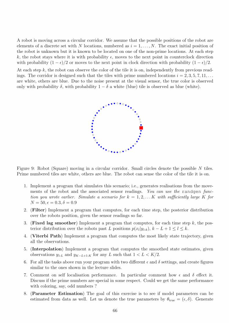
A robot is moving across a circular corridor. We assume that the possible positions of the robot areelements of a discrete set with N locations, numbered as i = 1, . . . , N . The exact initial position ofthe robot is unknown but it is known to be located on one of the non-prime locations. At each stepk, the robot stays where it is with probability ε, or moves to the next point in counterclock directionwith probability 1− ε.At each step k, the robot can observe the color of the tile it is on, independently from previous read-ings. The corridor is designed such that the tiles with prime numbered locations i = 2, 3, 5, 7, 11, . . .are white, others are blue. Due to the noise present at the visual sensor, with probability δ a white(blue) tile is observed as blue (white).

Figure 8: (Left) Robot (Square) moving in a circular corridor. Small circles denote the possible Ntiles. Prime numbered tiles are white, others are blue. The robot can sense the color of the tile it ison. (Right) The sensor can sense the color of two tiles in front.

1. Define the conditional probability tables given the verbal description above. Write a programthat generates one given N , δ and epsilon. Matlab has a function called isprime.

2. Implement a program that simulates this scenario; i.e., generates realisations from the move-ments of the robot and the associated sensor readings. You can use the randgen func-tion you wrote earlier. Simulate a scenario for k = 1, 2, . . . K with sufficiently large K forN = 50, ε = 0.3, δ = 0.9

3. (Optional) Implement a program that computes, for each time step, the posterior distributionover the robots position, given the sensor readings so far.

4. How many time steps are needed from the start on average until the location is known with90% certainty when δ = 0.99, provided the model is correct.

5. Suppose we modify the sensor such that it can sense the color of two tiles in front (in counter-clock direction), independent from each other and independent from previous readings. Definethe appropriate random variables.

Part II

65

A robot is moving across a circular corridor. We assume that the possible positions of the robot areelements of a discrete set with N locations, numbered as i = 1, . . . , N . The exact initial position ofthe robot is unknown but it is known to be located on one of the non-prime locations. At each stepk, the robot stays where it is with probability ε, moves to the next point in counterclock directionwith probability (1− ε)/2 or moves to the next point in clock direction with probability (1− ε)/2.

At each step k, the robot can observe the color of the tile it is on, independently from previous read-ings. The corridor is designed such that the tiles with prime numbered locations i = 2, 3, 5, 7, 11, . . .are white, others are blue. Due to the noise present at the visual sensor, the true color is observedonly with probability δ, with probability 1− δ a white (blue) tile is observed as blue (white).

Figure 9: Robot (Square) moving in a circular corridor. Small circles denote the possible N tiles.Prime numbered tiles are white, others are blue. The robot can sense the color of the tile it is on.

1. Implement a program that simulates this scenario; i.e., generates realisations from the move-ments of the robot and the associated sensor readings. You can use the randgen func-tion you wrote earlier. Simulate a scenario for k = 1, 2, . . . K with sufficiently large K forN = 50, ε = 0.3, δ = 0.9

2. (Filter) Implement a program that computes, for each time step, the posterior distributionover the robots position, given the sensor readings so far.

3. (Fixed lag smoother) Implement a program that computes, for each time step k, the pos-terior distribution over the robots past L positions p(xl|y1:k), k − L+ 1 ≤ l ≤ k.

4. (Viterbi Path) Implement a program that computes the most likely state trajectory, givenall the observations.

5. (Interpolation) Implement a program that computes the smoothed state estimates, givenobservations y1:L and yK−L+1:K for any L such that 1 < L < K/2.

6. For all the tasks above run your program with two different ε and δ settings, and create figuressimilar to the ones shown in the lecture slides.

7. Comment on self localisation performance. In particular comment how ε and δ effect it.Discuss if the prime numbers are special in some respect. Could we get the same performancewith coloring, say, odd numbers ?

8. (Parameter Estimation) The goal of this exercise is to see if model parameters can beestimated from data as well. Let us denote the true parameters by θtrue = (ε, δ). Generate

66

data from a model with K = 500 and N = 50, ε = 0.3, δ = 0.9. Compute the evidenceL(θ) = p(y1:K |θ) where θ is varied on a sufficiently dense grid on the unit square [0 1]2.Generate a contour plot of L(θ) and compare its peak with θtrue.

9. (Optional) Develop a numerical method for finding θ∗ = arg maxθ L(θ) without the exhaustivesearch.


67

Q53???: Adding Gaussian Random Variables

An important property of Gaussian random variables is that the sum is also Gaussian distributed.

x1 ∼ p1(x1) = N (x1;µ1, P1)

x2 ∼ p2(x2) = N (x2;µ2, P2)

y = x1 + x2

1. Using the Jacobian formula, show that

p(y) =

∫p1(x)p2(y − x)dx

(That is the convolution of p1 and p2).

2. A moment generating function is defined as

Mx(t) = 〈exp(tx)〉

Show that when two pdf’s are convolved, the resulting pdf has a moment generating functionthat is the product of the individual generating functions.

3. Derive the moment generating function for a Gaussian random variable with densityN (x;µ, P ).

4. Using the above results, show that y has a Gaussian distribution. Find the mean and varianceof y.


68

Q54???: Adding Poisson Random Variables

An important property of Poisson random variables is that the sum is also Poisson distributed.

x1 ∼ p1(x1) = PO(x1;µ1)

x2 ∼ p2(x2) = PO(x2;µ2)

y = x1 + x2

1. Show that

p(y) =∑x

p1(x)p2(y − x)

(That is the convolution of p1 and p2).

2. A probability generating function of a nonnegative discrete random variable is defined as

Gx(z) =∞∑t=0

p(x = t)zt

Show that when two pdf’s are convolved, the resulting pdf has a probability generating func-tion that is the product of the individual generating functions.

3. Derive the probability generating function for a Poisson random variable with density PO(x;µ).

4. Using the above results, show that y has a Poisson distribution. Find the mean and varianceof y.

5. Find the posterior distribution p(x1, x2|y).

6. Find the posterior marginal p(x1|y).


69

Q55?: Woodbury Formula

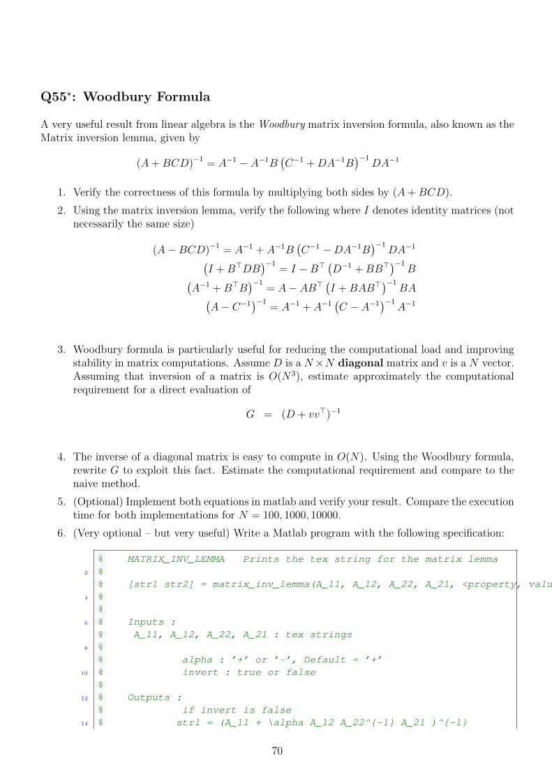
A very useful result from linear algebra is the Woodbury matrix inversion formula, also known as theMatrix inversion lemma, given by

(A+BCD)−1 = A−1 − A−1B(C−1 +DA−1B

)−1DA−1

1. Verify the correctness of this formula by multiplying both sides by (A+BCD).

2. Using the matrix inversion lemma, verify the following where I denotes identity matrices (notnecessarily the same size)

(A−BCD)−1 = A−1 + A−1B(C−1 −DA−1B

)−1DA−1(

I +B>DB)−1

= I −B>(D−1 +BB>

)−1B(

A−1 +B>B)−1

= A− AB>(I +BAB>

)−1BA(

A− C−1)−1

= A−1 + A−1(C − A−1

)−1A−1

3. Woodbury formula is particularly useful for reducing the computational load and improvingstability in matrix computations. Assume D is a N×N diagonal matrix and v is a N vector.Assuming that inversion of a matrix is O(N3), estimate approximately the computationalrequirement for a direct evaluation of

G = (D + vv>)−1

4. The inverse of a diagonal matrix is easy to compute in O(N). Using the Woodbury formula,rewrite G to exploit this fact. Estimate the computational requirement and compare to thenaive method.

5. (Optional) Implement both equations in matlab and verify your result. Compare the executiontime for both implementations for N = 100, 1000, 10000.

6. (Very optional – but very useful) Write a Matlab program with the following specification:

% MATRIX_INV_LEMMA Prints the tex string for the matrix lemma2 %

% [str1 str2] = matrix_inv_lemma(A_11, A_12, A_22, A_21, <property, value>)4 %

%6 % Inputs :

% A_11, A_12, A_22, A_21 : tex strings8 %

% alpha : ’+’ or ’-’, Default = ’+’10 % invert : true or false

%12 % Outputs :

% if invert is false14 % str1 = (A_11 + \alpha A_12 A_22^{-1} A_21 )^{-1}

70

% str2 = A_11^{-1} - alpha A_11^{-1} A_12 (A_{22}16 % + alpha A_21 A_11^{-1} A_{12})^{-1} A_21 A_11^{-1}

% if invert = true18 % str1 = (A_11^{-1} + \alpha A_12 A_22 A_21 )^{-1}

% str2 = A_11 - alpha A_11 A_12 (A_{22}^{-1}20 % + alpha A_21 A_11 A_{12})^{-1} A_21 A_11

%22 % Usage Example :

% matrix_inv_lemma(’D’, ’C^\top’, ’R’, ’C’, ’invert’, true, ’alpha’, ’-’)24 % ans =

% \left( D^{-1} - C^\top R^{-1} C \right)^{-1} =26 % D + D C^\top \left(R - C D C^\top \right)^{-1} C D

%28 %

% matrix_inv_lemma(’D’, ’C^\top’, ’R’, ’C’, ’invert’, false, ’alpha’, ’+’)30 % ans =

% \left( D + C^\top R C \right)^{-1} =32 % D^{-1} - D^{-1} C^\top \left(R^{-1} + C D^{-1} C^\top \right)^{-1} C D^{-1}

%


71

Q56???: Gaussian Process Regression

The goal of this exercise is to test your understanding of manipulations associated with multivariateGaussians. You may also find it helpful to read Bishop 6.4.

In Bayesian machine learning, a frequent problem that pops up is the regression problem where weare given a pairs of inputs xi ∈ RN and associated noisy outputs yi ∈ R. We assume the followingmodel

yi ∼ N (yi; f(xi), R)

The interesting thing about a Gaussian process is that the function f is not specified in close form,but we assume that the function values

fi = f(xi)

are jointly Gaussian distributed as f1...fL

= f1:L ∼ N (f1:L; 0,Σ(x1:L))

Here, we define the entries of the covariance matrix Σ(x1:L) as

Σi,j = K(xi, xj)

for i, j ∈ {1, . . . , N}. Here, K is a given covariance function. Now, if we wish to predict the value off for a new x, we simply form the following joint distribution:

f1...fLf

∼ N ((f1:L, f); 0,Σ(x1:L, x))

Here, Σ(x1:L, x) is a L+ 1 by L+ 1 covariance matrix with entries

Σi,L+1 = ΣL+1,i = K(xi, x) = K(x, xi)

72

−3 −2 −1 0 1 2 3 4 50

2

4

6

8

10

12

14

16

x

f

Data

Prediction

Error bars

−3 −2 −1 0 1 2 3 4 50

2

4

6

8

10

12

14

16

x

f

Data

Prediction

Error bars

Figure 10: Gaussian Process Regression. Result obtained with a Bell shaped K1 (Top) and Laplacian(Bottom) covariance function.

Popular choices of covariance functions to generate smooth regression functions include a Bell shapedone

K1(xi, xj) = exp

(−1

2‖xi − xj‖2

)and a Laplacian

K2(xi, xj) = exp

(−1

2‖xi − xj‖

)

73

1. Derive the expressions to compute the predictive density

p(y|y1:L, x1:L, x)

2. Write a program to compute the mean and covariance of p(y|y1:L, x1:L, x) to generate figureslike Figure 10 for the following data:

x = [-2 -1 0 3.5 4]’;y = [4.1 0.9 2 12.3 15.8]’;

Try different covariance functions and observation noise covariances R and comment on thenature of the approximation.

3. Suppose we are using a covariance function parameterised by

Kβ(xi, xj) = exp

(− 1

β‖xi − xj‖2

)Find the optimum regularisation parameter β∗(R) as a function of observation noise variancevia maximisation of the marginal likelihood, i.e.

β∗ = p(y1:N |x1:N , β, R)

Generate a plot of b∗(R) for R = 0.01, 0.02, . . . , 1 for the dataset given in 2.


74

Q57?: Partitioned Inverse Equations

We partition a matrix Z as

Z =

(A BD C

)and define the Schur complements of Z with respect to this partitioning as

M =(A−BC−1D

)N =

(C −DA−1B

)Verify the following

1.

Z−1 =

(M−1 −M−1BC−1

−C−1DM−1 C−1 + C−1DM−1BC−1

)

2.

Z−1 =

(A−1 + A−1BN−1DA−1 −A−1BN−1

−N−1DA−1 N−1

)


75

Q58???: Multivariate Gaussian Distribution

A convenient property of the multivariate Gaussian distribution is that its marginals and conditionalsare Gaussians, hence can be expressed by a mean and a covariance parameter. In this exercise, wewill investigate these important properties.

Consider the joint distribution over the variable

x =

(x1x2

)where the joint distribution is Gaussian p(x) = N (x;µ,Σ) where

µ =

(µ1

µ2

)Σ =

(Σ1 Σ12

Σ>12 Σ2

)1. (Conditionals) Find the following

a) p(x1|x2)b) p(x2|x1)

2. (Marginals) Find

a) p(x1)

b) p(x2)

Using the partitioned inverse equations, you need to rearrange

p(x1, x2) ∝ exp

(−1

2

(x1 − µ1

x2 − µ2

)>(Σ1 Σ12

Σ>12 Σ2

)−1(x1 − µ1

x2 − µ2

))

bring the expression in form of p(x1)p(x2|x1) (or p(x2)p(x1|x2)) where the marginal andconditional can be easily identified. See also Bishop, section 2.3.


76

Q59??: Prediction and Update Equations

Consider the following model:

x0 ∼ N (x0;µ0,Σ0)

x1|x0 ∼ N (x1;Ax0, Q)

y1|x1 ∼ N (y1;Cx1, R)

1. Draw the graphical model

2. Find the following quantities and express them as Gaussian Distributions in moment parametri-sation

a) p(x1)

b) p(x0, x1)

c) p(y1)

d) p(x1|y1)e) p(x0, x1|y1)


77

Q60?: Multiplication of Gaussian Kernels

Express

G(x) = K1(x)K2(x)

in form eαN (x;µ,Σ) where for i = 1, 2

1. Ki = N (x; 0, 1)

2. Ki = N (x; 0, Pi)

3. Ki = N (x;µi, 1)

4. Ki = N (x;µi, Pi)


78

Q61??: Log-partition Function and Its Derivatives

We call a probability distribution with density p(x; θ) on a set X n ⊂ Rn an exponential family1 if ithas the following functional form

p(x; θ) = exp(θ>φ(x)− A(θ))∫Xn

dx p(x; θ) = exp(−A(θ))

∫Xn

dx exp(θ>φ(x)) = 1

A(θ) = log

∫Xn

dx exp(θ>φ(x))

• The elements of the vector θ are known as exponential or canonical parameters.

• The functions φ(x) are the sufficient statistics.

• The function A(θ) is known as the log partition function or the cumulant generating functionand ensures that the distribution normalizes to one. The log-partition function is definedthrough an integral. Hence we have to ensure that this integral exists (i.e. is finite). We definethe set of valid parameters as Θ ≡ {θ|A(θ) <∞}

We already know that many well-known distributions belong to an exponential family. The deriva-tives of A(θ) provide the cumulants of the distribution2.

1. Show that

∂

∂θA(θ) = 〈φ(x)〉p(x;θ)

i.e., the derivative of the log-partition function gives the expected sufficient statistics

2. Show that the Hessian (the matrix of second derivatives) is given as

∂2

∂θ∂θ>A(θ) =

⟨φ(x)φ(x)>

⟩− 〈φ(x)〉〈φ(x)〉>

This latter equation, by Jensen’s inequality shows that the Hessian is always positive definite,hence A(θ) is convex.

3. Express the following distributions as an exponential family, identify the log partition functionA(θ) and the canonical parameters θ, and by calculating the derivatives of A(θ), find theexpected sufficient statistics

a) Gaussian N (x;µ,Σ)

b) Gamma G(x; a, b)

c) Beta B(x;α, β)

d) Bernoulli BE(x; π)

1Note that in the lecture we gave a slightly more general definition of an exponential family including a scalingfunction h(x).

2The mean is the first cummulant, the covariance is the second cumulant e.t.c. The term “cumulant” come fromthe fact that when two independent random variables are added, their cumulants are added (accumulated), too. Notethe subtle difference between a moment generating function which is defined as 〈exp(θx)〉p(x).

79

e) Poisson P(x;λ)


80

Q62??: Gibbs Sampler For One Sample Source Separation

In this exercise you will implement a Gibbs sampler for a toy model described in the lecture.

s1 ∼ p(s1) = N (s1;µ1, P1)

s2 ∼ p(s2) = N (s2;µ2, P2)

x|s1, s2 ∼ p(x|s1, s2) = N (x; s1 + s2, R)

1. Derive an expression for the exact posterior p(s1, s2|x) when Pi, µi andR are known parametersfor i = 1, 2.

2. Derive the full conditionals p(s1|s2, x) and p(s2|s1, x)

3. Implement a Gibbs sampler. We will use the following parameters: µ1 = 3, µ2 = 5,P1, P2 = 0.5 and R = 0.3. Monitor the convergence of ergodic averages to the exact meanand covariance. How many iterations does it take until the posterior mean and covariance arecorrect 5% if s(0) = (µ1, µ2)?.

4. Repeat the previous experiment with R = 0.005. How many iterations does it take untilconvergence if s(0) = (µ1, µ2)? This should illustrate the fact that when two variables arestrongly correlated the Gibbs sampler moves very slowly.


81

Q63???: Sampling For Gaussians

Given the model

x0 ∼ N (x0; 0,Σ)

x1|x0 ∼ N (x1;Ax0, Q)

where

N (x;µ,Σ) ≡ |2πΣ|−1/2 exp

(−1

2(x− µ)>Σ−1(x− µ)

)is the multivariate Gaussian distribution, A,Q and Σ are known matrices.

1. Find the joint distribution p(x0, x1) and express it as a multivariate Gaussian using blockmatrices.

2. Using the block matrix inverse equations, find a factorisation of p(x0, x1) as p(x1)p(x0|x1) andexpress the factors as Gaussian distributions.

3. Assume now that we observe y where

y|x1 ∼ N (y;Cx1, R)

Find an expression for p(x0, x1|y).

4. Derive the full conditionals p(x0|x1, y) and p(x1|x0, y)

5. Implement a Gibbs sampler to sample from p(x0, x1|y).

6. Implement a rejection sampler to sample from p(x0, x1|y) using Mp(x0, x1) as the proposal,where M is a suitable positive number. Compute the rejection ratio.

7. Implement an importance sampler to sample from p(x0, x1|y) using p(x0, x1) as the proposal.


82

Q64???: Transition Kernels

x1 and x2 are two discrete random taking values in the discrete set X . Suppose we have the jointdistribution given as a table φa,b where π(x) = p(x1 = a, x2 = b) = 1

Zφa,b.

Suppose we implement a Metropolis algorithm to sample from this target distribution with thefollowing proposal technique: Given the current configuration x(n) = (x

(n)1 , x

(n)2 ), for each n, we

choose an index i(n) ∈ {1, 2} randomly with probability 0.5 and choose xi(n) according to a uniformdistribution.

1. Implement a Metropolis algorithm using the above proposal mechanism

2. Write down the state transition diagram of the proposal distribution and indicate the statetransition probabilities,

3. Write a program to compute the acceptance probability and the transition Kernel TM of thisMetropolis algorithm. Verify the results of your program for φ−1,−1 = φ1,1 = 3, φ−1,1 =φ1,−1 = 0.2. The transition kernel will be a 4× 4 matrix. If you are programming in Matlab,you may consider using 4−D arrays and the function reshape.

4. (Optional) Verify numerically if detailed balance condition is satisfied by this particularMetropolis algorithm (i.e., if TM(x|x′)π(x′) = TM(x′|x)π(x)).

5. Implement a deterministic scan Gibbs sampler (that is we sample alternatingly from the fullconditional distributions p(x1|x2) and p(x2|x1)).

6. Write a program to compute the Gibbs transition Kernel TG. Verify the results of yourprogram for φ−1,−1 = φ1,1 = 3, φ−1,1 = φ1,−1 = 0.2.

7. Using eigenvalue decomposition of TG and TM , estimate which transition kernel will convergefaster to the stationary distribution.


83

Q65?: Factorization of Probability Tables

Consider the following probability table

p(x1, x2) x2 = 0 x2 = 1x1 = 0 1/10 3/10x1 = 1 2/10 4/10

1. Factorise this table as

a) p(x1)p(x2|x1)b) p(x2)p(x1|x2)

2. Suppose we would like to enforce a new prior p∗(x1) for this probability table such that

p∗(x1) =∑x2

p∗(x1, x2)

We let

p∗(x1, x2) =p∗(x1)

p(x1)p(x1, x2)

This operation can be interpreted as multiplying-in a new prior. Suppose p∗(x1) = [0.5 0.5].Find the new table p∗(x1, x2).


84

Q66??: Gibbs sampler for the AR model

In this problem, you will develop a Gibbs sampler for an AR model:

A ∼ N (A; 0, 1.2)

R ∼ IG(R; 0.4, 250)


x0 = 1 x1 = −6

N (x;m, r) = exp{−1

2(x2 +m2 − 2xm)/r − 1

2log(2πr)}

IG(r; a, b) = exp

(−(a+ 1) log r − 1

br− log Γ(a)− a log b

)

1. Write the expression for the full joint distribution and assign terms to the individual factorson the factor graph

p(A,R|x0, x1) ∝ p(x1|x0, A,R)p(A)p(R)

= N (x1;Ax0, R)N (A; 0, P )IG(R; ν, β/ν)

∝ exp

(−1

2

x21R

+ x0x1A

R− 1

2

x20A2

R− 1

2log 2πR

)exp

(−1

2

A2

P

)exp

(−(ν + 1) logR− ν

β

1

R

)2. Derive the full conditional distributions p(A|R, x0, x1) and p(R|A, x0, x1) The result should be

p(A|R, x0, x1) = N (A;µA,ΣA)

ΣA =

(x20R

+1

P

)−1µA = ΣA

x0x1R

p(R|A, x0, x1) = IG

(R; ν +

1

2,

(1

2(x1 − Ax0)2 +

ν

β

)−1)

3. Implement the Gibbs sampler and plot the results

The Matlab code is given below. To generate an inverse gamma random variable, we used1/(b gamrnd(a))

85

beta_nu = 250; nu = 0.4; P = 1.2; x_0 = 1; x_1 = -6; T = 10000;2 R = zeros(1, T); A = zeros(1, T);

A(1) = -6; R(1) = 0.00001;4

for t=2:T,6 Sig = 1/(x_0ˆ2/R(t-1) + 1/P);

mu = Sig*x_0*x_1/R(t-1);8 A(t) = sqrt(Sig)*randn + mu;

10 b = 0.5*(x_1 - A(t)*x_0).ˆ2 + 1/beta_nu;R(t) = 1/(gamrnd(nu+0.5, 1/b));

12 end;

4. Implement the simulated annealing and iterative improvement to find the mode of the posteriorp(A,R|·). The mode of an inverse gamma distribution is at r = 1/((a+ 1)b).


86

Q67?: Sampling from Multivariate Gaussians

Consider a Gaussian random vector y ∈ RN . We wish to generate samples from this distributionusing independent Gaussians.

1. Let z ∈ RN

z ∼ N (z; 0, IN)

Show that, if

y = Wz + µ

where Σ = W>W , then

y ∼ N (y;µ,Σ)

2. Write a program that generates samples from N (y;µ,Σ).

3. Suppose we wish to set some elements of the vector y indexed by α are set to known valuesgiven by yα, i.e.,

y =

(yαy−α

)For example, if N = 4 and α = {1, 4}, then −α = {2, 3}. Derive the conditional distributionof y−α and write a program, that given µ and Σ samples y such that yα = yα.


87

Q68??: Resampling

In the literature, there are several resampling methods. The most popular are

• Multinomial Resampling

• Systematic Resampling

• Residual Resampling

In this exercise, we will implement and investigate these techniques.

1. Multinomial resampling is equivalent to sampling histograms with N bins where each bin hasprobability w(i) for i = 1 . . . N and

∑i w

(i) = 1. The algorithm is as follows:

• uk ∼ U(uk; 0, 1) (uniform in [0, 1]) for k = 1 . . . N

• Define intervals

Ii =

(i−1∑j=1

w(j),i∑

j=1

w(j)

]

• Count number of u that fall into the interval Ii

Ni =∑k

[uk ∈ Ii]

This procedure is equivalent to sampling from a Multinomial distribution

N1:N ∼ M(N1:N ; w(i), N)

and is shown in Fig 11. Implement a program for multinomial resampling. It is possible to do

1 2 3 4 5 60

0.1

0.2

0.3

0.4

w(i) (

Norm

alis

ed w

eig

hts

)

1 2 3 4 5 60

0.5

1

u1

uk

1 2 3 4 5 60

0.5

1

1.5

2

i (Particle Index)

Ni (

Counts

)

Figure 11: Sampling from a Multinomial

this in two lines of Matlab code using the histc function.

2. Systematic resampling is very similar to multinomial sampling but the u are chosen as follows:

88

1 2 3 4 5 60

0.1

0.2

0.3

0.4

w(i) (

Norm

alis

ed w

eig

hts

)

1 2 3 4 5 60

0.5

1

u1

uk

1 2 3 4 5 60

0.5

1

1.5

2

i (Particle Index)

Ni (

Counts

)

Figure 12: Systematic Resampling

• u1 ∼ U(u1; 0, 1/N) (uniform in [0, 1/N ])

• uk = u1 + (k − 1)/N for k = 2 . . . N

and is shown in Fig 12. Implement a program for systematic resampling.

3. Residual resampling works as follows

• Every bin is assigned first a fixed number of off-springs proportional to its weight

Ni = bNw(i)c

• Calculate the “residual” weights and normalise

W (i) = w(i) − Ni/N

w(i) = W (i)/∑i′

W (i′)

• Sample from the residual N = N −∑

i Ni

N1:N ∼ M(N1:N ; w(i), N)

An illustration is shown in Fig 13. Implement a program for residual resampling.

4. For each method, given N = 10 and w(i) ∝ i/N for i = 1 . . . N estimate by simulation themean and the variance of the Monte Carlo error

Ni − w(i)N

Conclude which resampling method is a better choice. The means should be very close tozero as these methods are unbiased. The variances for multinomial resampling are around0.18, 0.35, 0.51, 0.66, 0.83, 0.97, 1.11, 1.25, 1.37, 1.48 and for systematic resampling 0.15, 0.23, 0.25, 0.20, 0.08, 0.08, 0.20, 0.25, 0.23, 0.15.


89

1 2 3 4 5 60

0.1

0.2

0.3

0.4

1/N

k/N

w(i) (

Norm

alis

ed w

eig

hts

)1 2 3 4 5 6

0

0.5

1

1.5

2

i (Particle Index)N

i (C

ounts

)

Figure 13: Residual Resampling

Q69???: Kalman Filter, Particle Filter

Consider the following linear dynamical model for t = 1, 2, . . . ,

st =

(1 ∆0 1

)st−1 + wt

yt =(

1 0)st + εt

Here, wt and εt are independent and

s0 ∼ N (s0; 0, P )

wt ∼ N (wt; 0, Q)

εt ∼ N (εt; 0, R)

1. Draw the graphical model for this process.

2. Write a program that would generate y1:T and st given T, P,Q,R and ∆. How do the typicaltrajectories look like for P = 1, Q = 0.01, R = 0.1, ∆ = 1/2? What happens when ∆ ischanged?

3. Derive an algorithm for computing the mean and covariance matrix of p(st|y1:t) for each trecursively. This is the Kalman filtering recursion

4. Write a Matlab program to visualise the exact filtering density. You can plot equal probabilityellipses as shown in the lectures.

5. Implement a sequential Monte Carlo algorithm to estimate the mean and the variance ofp(st|y1:t) using the state transition distribution as the proposal.


90

Q70??: Hidden Markov Model

Implement the correction smoother to compute p(xt|y1:T ) for the following HMM with yt ∈ 0, 1 andxt ∈ a, b, c:

p(y1:T , x0:T ) = p(x0)T∏t=1

p(yt|xt)p(xt|xt−1)

Note that this setup is slightly different from the model discussed in the class that due to x0. Use thefollowing parameters:

p(xt = i|xt−1 = j) = Ai,j

A =

0.9 0 0.30.1 0.8 00 0.2 0.7

p(yt = k|xt = i) = Bk,i

B =

(0.99 0.6 0.010.01 0.4 0.99

)p(x0) ∼ U [′,∞]

Verify your results by comparing with the forward-backward algorithm on the following observationsequence:

y1:12 = [0001m110mm01]

where m means missing data. The results for both algorithms must be identical.


91

Q71???: Variational Bayes for Changepoint Model

Consider the following changepoint model:

λ0 ∼ G(λ0; a, b0)

rt ∼ BE(rt; π1) π0 = 1− π1λt|rt, λt−1 ∼ δ(λt − λt−1)[rt=0]G(λt; a,B)[rt=1]

xt|λt ∼ PO(xt;λt)

Here, rt ∈ Dr = {0, 1} and λt ∈ R+. The symbols G, BE and PO denote the gamma, Bernoulli andthe Poisson distribution respectively

G(λ; a, b) = exp ((a− 1) log λ− bλ− log Γ(a) + a log b)

BE(r; π) = exp (r log π + (1− r) log(1− π))

PO(x;λ) = exp (x log λ− λ− log Γ(x+ 1))

In the class, we have assumed that the parameters a, b0 and B are known. In practice we don’t knowthese.

• Assume that a and b0 are known but

B ∼ G(B; 1, 10)

1. Draw the associated graphical model

2. Derive and implement an EM algorithm to find B∗ = arg maxB p(r1:T , λ1:T , B|x1:T )

3. Derive a variational Bayes algorithm that approximates p(r1:T , λ1:T , B|x1:T ) by q(r1:T , λ1:T )q(B).Choose a gamma density for q(B).

Note that the algorithms will be very similar where EM learns a single parameter whereasVB estimates a distribution on B. Test your algorithms on the coal mining disaster datasetgiven as

4 5 4 1 0 4 3 4 0 6 3 3 4 0 2 6 3 3 5 4 5 3 1 4 4 1 5 5 3 4 2 5 2 2 3 4 2 1 3 2 2 1 1 1 1 3 0 0 1 01 1 0 0 3 1 0 3 2 2 0 1 1 1 0 1 0 1 0 0 0 2 1 0 0 0 1 1 0 2 3 3 1 1 2 1 1 1 1 2 4 2 0 0 0 1 4 0 0 01 0 0 0 0 0 1 0 0 1 0 1

Show clearly the posterior probability of the changepoints.


92

Q72???: Kalman Filtering and Smoothing

In this question, we will investigate the Kalman filter and the Kalman smoother for interpolation ofsignals.

Suppose we are given a noisy signal y0:T−1 ≡ (y0, y1, . . . , yT−1). Furthermore, suppose that somesample values are missing at time indices t ∈ I, where I is a known set.

We will use the following linear dynamical system

x0 ∼ N (0, S)

xt|xt−1 ∼ N (xt;Axt−1, Q)

yt|xt ∼ N (Cxt, R)

Here, S = 1000I2, Q = 0.001I2 and R = 0.5. The transition model

C =√

2(

1 0)

A = exp(−ρ)

(cos(ω) − sin(ω)sin(ω) cos(ω)

)1. Write a program to generate data from this LDS given ω and ρ. By investigating different

values and the associated realisations, explain the model.

2. Assume that yt are missing for t ∈ {L . . . T −L−1} = I. Use the Kalman filter and smootherto estimate p(yt|y−I) for t ∈ I. Plot your results (the mean and the variance as 3σ error bars)for T = 100 and L = 3, 10 and 30.

0 10 20 30 40 50 60 70 80 90 100−50

0

50

3. In the above, we have assumed that the parameters are known. This is often not the casein practice. Devise and implement a method based on the Kalman filter to estimate the MLsolution for ω and ρ. Consider computing the loglikelihood for a grid of ρ and ω.

4. Assume we are given the following sequence y1:12 = [−300,−330,m,m,m,m,m,m,m,m, 250, 280].Find the mean and the variance of p(yt|y1:2, y11:12, ω∗, ρ∗) for t = 2 . . . 10.


93

Q73???: Clustering with Missing ValuesSuppose we are given the following dataset in the left column, where NaN’s denote missing values.In this question, you will only use the dataset with missing values; the complete dataset is forcomparison only. Here, each row is a point on R2.

Dataset Without MissingNaN -0.3742 1.2762 -0.3742NaN 3.1832 -0.0999 3.1832

-0.6887 NaN -0.6887 2.62772.2469 NaN 2.2469 -0.1871

-0.8456 NaN -0.8456 1.7727NaN 0.8245 -0.0694 0.8245

0.1537 NaN 0.1537 1.3422-0.0754 NaN -0.0754 2.2690-0.7237 NaN -0.7237 1.7694

NaN 0.5313 0.2801 0.5313NaN 3.9396 0.8288 3.9396

2.7675 NaN 2.7675 -0.2526NaN 1.1712 0.3429 1.1712NaN 2.7526 1.5023 2.7526

0.6299 NaN 0.6299 1.29932.2560 NaN 2.2560 -0.44661.7509 NaN 1.7509 -0.4560

-0.8206 NaN -0.8206 1.2730NaN 0.6409 -0.1679 0.6409NaN -0.0942 2.4861 -0.0942

0.5593 NaN 0.5593 2.2157NaN -1.1865 2.3954 -1.1865

-0.8162 NaN -0.8162 1.64240.0877 NaN 0.0877 2.9030

-0.2320 NaN -0.2320 3.00922.3803 NaN 2.3803 0.93932.1016 NaN 2.1016 -0.5255

-1.1851 NaN -1.1851 2.1244NaN 1.7659 0.6548 1.7659NaN 1.7531 -0.4326 1.7531

-0.8773 NaN -0.8773 1.6056-0.1446 NaN -0.1446 2.0367

NaN 2.4891 -0.0510 2.48910.0875 NaN 0.0875 3.4512

NaN 3.4436 0.2496 3.4436-0.5785 NaN -0.5785 2.4212-0.2082 NaN -0.2082 2.4801

NaN 0.2512 0.4751 0.2512NaN -1.1528 0.9384 -1.1528NaN 3.1762 0.3215 3.1762

1. Suppose we believe that data comes from a mixture of Gaussians with K = 2 components,with different mean vectors µ1 and µ2 and a diagonal covariance matrix Σ = diag(sx, sy) thatis shared by both components. Develop a Bayesian model for this scenario, define appropriatepriors and conditional distributions and sketch a graphical model.

2. Write the mathematical expression for the joint density

3. Develop an EM algorithm to estimate the MAP values of µ1, µ2 and Σ given the dataset.

4. Develop an algorithm to predict the missing values and the posterior probability of componentlabels (for K = 2) for each data point. Compute the mean of your prediction and the errorbars (as given by the standard deviation of the predictive distribution for the missing values).Comment on the quality of the predictions.

5. Sketch a variational Bayes algorithm, along Bayesian model selection principles, to estimatethe most likely number of components, when K is unknown.


94

Q74???: ChangepointSuppose we observe the following dataset xt ∈ 0, 1 for t = 1 . . . 50

0 0 1 0 0 1 0 0 0 0 1 0 0 0 0 1 0 0 1 0 1 1 0 0 1 1 1 1 1 1 1 1 1 1 1 0 1 1 0 1 1 1 1 1 1 1 1 1 1 1

1. Suppose we know that the data comes from the following model

π1 ∼ B(1, 1)

π2 ∼ B(1, 1)

xt ∼{BE(xt; π1), t <= nBE(xt; π2), t > n

2. Derive, compute and plot the posterior probability of p(n|x1:50) given that n is a-priori uni-form.


95

Q75??: Factorizing Gaussians

Given the model

x0 ∼ N (x0; 0,Σ)

x1|x0 ∼ N (x1;Ax0, Q)

where

N (x;µ,Σ) ≡ |2πΣ|−1/2 exp

(−1

2(x− µ)>Σ−1(x− µ)

)is the multivariate Gaussian distribution, A,Q and Σ are known matrices.

1. Find the joint distribution p(x0, x1) and express it as a multivariate Gaussian.

2. Find a factorisation of p(x0, x1) as p(x1)p(x0|x1) and express the factors as Gaussian distri-butions.


96

Q76???: Metropolis and Gibbs

x1 and x2 are two discrete random variables taking values in {−1, 1}. Suppose we have the jointdistribution p(x1 = a, x2 = b) = πa,b. We further have g = π−1,1 = π1,−1 > π1,1 = π−1,−1.

Suppose we implement a Metropolis algorithm to sample from this target distribution with thefollowing proposal technique: Given the current configuration x(n) = (x

(n)1 , x

(n)2 ), for each n, we

choose an index i(n) ∈ {1, 2} randomly with probability 0.5 and flip the sign of xi(n) .

1. Write down the state transition diagram of the proposal distribution and indicate the statetransition probabilities,

2. Find an expression for the acceptance probability as a function of g,

3. Write the pseudocode for the Metropolis sampler,

4. Write down the state transition diagram of the transition Kernel TM of this Metropolis algo-rithm and indicate the transition probabilities,

5. Verify if detailed balance condition is satisfied by this particular Metropolis algorithm (i.e., ifTM(x|x′)π(x′) = TM(x′|x)π(x)) for all values of g.

6. Suppose we also implement a deterministic scan Gibbs sampler (that is we sample alternatinglyfrom the full conditional distributions p(x1|x2) and p(x2|x1)). Write down the pseudocode.

7. Write down an expression for the Gibbs transition Kernel TG in terms of g.

8. Verify detailed balance is satisfied the Gibbs transition Kernel TG for all values of g.


97

Q77??: Variational Methods

Consider the following probability tables

p(x1, x2) x2 = 0 x2 = 1x1 = 0 π0,0 π0,1x1 = 1 π1,0 π1,1

q(x1, x2) x2 = 0 x2 = 1x1 = 0 (1− q1)(1− q2) (1− q1)q2x1 = 1 q1(1− q2) q1q2

By minimising KL(q||p), show that the solution satisfies the relation

q(x1) ∝ exp{〈log p〉q(x2)}q(x2) ∝ exp{〈log p〉q(x1)}


98

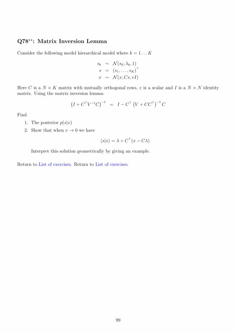
Q78??: Matrix Inversion Lemma

Consider the following model hierarchical model where k = 1 . . . K

sk ∼ N (sk;λk, 1)

s = (s1, . . . , sK)>

x ∼ N (x;Cs, vI)

Here C is a N ×K matrix with mutually orthogonal rows, v is a scalar and I is a N × N identitymatrix. Using the matrix inversion lemma:(

I + C>V −1C)−1

= I − C>(V + CC>

)−1C

Find

1. The posterior p(s|x)

2. Show that when v → 0 we have

〈s|x〉 = λ+ C>(x− Cλ)

Interpret this solution geometrically by giving an example.


99

Q79???: Interpolation via EM

Consider a Markov chain,

p(x1)p(x2|x1)p(x3|x2)

where the transition and initial state probabilities are given by p(xt = i|xt−1 = j) = Ai,j andp(x1 = i) = πi. Assume that t = 1, 2, 3 only and π are known.

Suppose we observe N realisations from the model. However, for n = 1 . . . N , we observe x1 = x(n)1

and x3 = x(n)3 but all the observations for x2. How can we estimate the transition matrix Ai,j?.

This is a typical setting for the EM algorithm where the observations are x1 and x3, the missing dataare x2 and the unknown parameters are π and A.

1. Draw the graphical models for this inference problem

2. Write down the complete data loglikelihood log p(x1:3|π,A)

3. Show how to compute the E-step

p(x(n)2 |x

(n)1 , x

(n)3 )

4. In the M step, find the energy term

F(θ; θ(τ)) = 〈log p(x1:3|π,A)〉

and in order to maximize w.r.t. As,j, form the Lagrangian and take the derivative and set tozero. Show that this leads to the result

Ai,j =

∑n

(⟨[i = x

(n)2

]⟩ [j = x

(n)1

]+[i = x

(n)3

] ⟨[j = x

(n)2

]⟩)∑

s

∑n

(⟨[s = x

(n)2

]⟩ [j = x

(n)1

]+[s = x

(n)3

] ⟨[j = x

(n)2

]⟩)5. The following Matlab code generates data from the model

% Number of sequences2 N = 100;

% Number of time slices4 T = 3;

S = 2;6 A_true = [0.9 0.1;0.3 0.7]’;

pi_true = [0.4 0.6];8 data.x = zeros(N, T);

% Generate data10 for n=1:N,

for t=1:T,12 if t==1,

data.x(n, t) = randgen(pi_true);14 else

data.x(n, t) = randgen(A_true(:,data.x(n, t-1)));

100

16 end;end;

18 end;

The following code contains the skeleton of the EM algorithm. Fill in the M step

%% EM algorithm2 %% We pretend that data.x(:, 2) are missing

%% We only estimate A4

A = 0.5*ones(2);6 p_x2 = zeros(S, N);

for ep=1:100,8 % E step

for n=1:N,10 Z = A(data.x(n, 3), :)*A(:, data.x(n, 1));

p_x2(:, n) = A(data.x(n, 3), :)’.*A(:, data.x(n, 1))./Z;12 end;

% logLikelihood computation14 LL = zeros(1, N);

for n=1:N,16 LL(n) = log(A(data.x(n, 3), :)*A(:, data.x(n, 1))) ...

+ log(pi_true(data.x(n, 1))) ;18 end;

lk = sum(LL);20

% M step22 .... <Fill in>

24

A26 lk % the likelihood must increase monotonically!

pause28 end;


101

Q80??: A Probability Table

The goal of this exercise is to investigate sampling algorithms and variational algorithms on a toyexample and provide warm up for the following exercises.

Suppose we are given a N1 ×N2 table L where the entry at i’th row and j’th column denotes

Li,j = log p(x1 = i, x2 = j) + logZ

where p(x1, x2) is the joint distribution of x1, x2 with x1 ∈ {1, . . . , N1} and x2 ∈ {1, . . . , N2} and Zis an unspecified positive constant.

1. Write a program to compute the “variational marginals”, i.e., two distributions q1(x1) andq2(x2) such that

KL(q1q2||p)

is minimised.

2. Compare the “variational marginals” with the exact marginals p(x1) and p(x2) given L.

3. Derive the update equations of an EM algorithm to compute

x∗1 = argmaxx1

∑x2

p(x1, x2)


102

Q81??: A Chain

Suppose we are given a probability distribution that factors according to

p(x0, . . . , xT ) =1

Zexp

(T∑t=1

ψ(xt−1, xt)

)

We know that xt ∈ {1, . . . , N}1. Describe a procedure to compute Z and the marginals p(xt) for t = 0, . . . , T exactly. Write

a program to compute logZ and log p(xt) for t = 0, . . . , T given ψ(xt−1 = i, xt = j) as aN × N × T array with psi(i, j, t). Draw the factor graph and observe the similaritiesto the HMM derivation given in the lectures.

2. Derive an algorithm to compute the Viterbi path

x∗0:T = argmaxx0:T

p(x0, . . . , xT )

and write a program to compute it.

3. Derive a simulated annealing (SA) algorithm to sample from

1

Z βexp

(β

T∑t=1

ψ(xt−1, xt)

)= pβ(x0, . . . , xT )

where β is an inverse temperature variable. Design an annealing schedule β →∞ to computethe Viterbi path. Compare your solutions to the exact solution.

4. Derive a variational Bayes algorithm that uses a fully factorised approximating distribution

Q =T∏t=0

q(xt)

Derive the update equations and implement the algorithm. Compare the variational marginalsto the true marginals.

5. Derive the variational lower bound and write an algorithm to compute it. Compare to theexact logZ you have computed earlier. Show with a plot that it is strictly increasing duringthe iterations.

6. The variational method can also be used to compute the Viterbi path by targeting pβ withβ →∞. Using the same schedule as the SA, compare if you find better solutions with annealedVB. The solutions can be compared according to the number of mismatches with the truetrajectory and the probability that the solution achieves.


103

Q82??: Bayesian Estimation of Gaussians

Consider the following model

β ∼ G(β; ν, 1)

µ ∼ N (µ; 0, 1000)

xi ∼ N (xi;µ, β−1)

for i = 1 . . . N . Suppose we are given the following dataset

x1,6 = {−6, −1, −0.2, 0.1, 2, 4} ≡ X

1. Derive and implement a Gibbs sampler to sample from

p(µ, β|X, ν = 0.1)

2. Derive and implement a variational Bayes algorithm to approximate p(µ, β|ν = 0.1, X). Takeas the approximating distribution a factorised distribution Q = q1q2 where

q1(β) = G(β; a, b)

q2(µ) = N (µ;m,Σ)

3. How would you find

ν∗ = argmaxν

p(x1:N |ν)

i.e., the ML estimate of ν? Explain.


104

Q83????: Movie Rating

A popular model for collaborative filtering for recommender systems is based on matrix factorization.Here, a matrix X (with possibly a lot of missing entries) represents, for example, the ratings xij ofusers i for movie j. If we can assume that the actual X is low rank, there is hope for reconstruction ofthe missing elements. Consider the following model that assumes X ≈ wh>, i.e., X is approximatedwell with a rank one matrix:

xij ∼ PO(xij;wihj)

mij =

{1 if xij is observed0 if xij is not observed

hj ∼ G(hj;α, β) = exp((α− 1) log hj − βhj − log Γ(α) + α log β)

wi ∼ G(wi;α, β) = exp((α− 1) logwi − βwi − log Γ(α) + α log β)

where

i = 1 . . . I

j = 1 . . . J

and hj is the jth movie’s rating independent of users’ opinion; wi, the ith user’s tendency; and xij,jth movie’s rating by the user i. The matrix M of mij denotes the known (if 1) and the missing data(if 0).

Generate a synthetic data set X = {xij} with I = 50 and J = 20. Sample the true w and h valuesfrom a gamma distribution with parameters α = 0.5 and β = 0.1. Sample the mask matrices Mq

from Bernoulli distributions with parameters q = 0.1, 0.2, . . . , 0.9. Our goal will be to predict foreach q the same missing entries, corresponding to zero elements of M0.9 only. Intuitively, providedthat the model is correct, the more data points there are, the better our predictions should be. Wewill measure the accuracy of our predictions by MSE (mean square error) defined as

MSE(X) =∑

i,j s.t. M0.9(i,j)=0

(xij − xij)2/∑

i,j s.t. M0.9(i,j)=0

1

where X is the prediction generated by the model.

To generate the masksMq consistently for all q, you can use the Matlab code: q = 0.1:0.1:0.9;rM = rand(I,J); for u=1:9, M = (rM < q(u)); ... end; .

1. Derive and implement an ICM algorithm for the model to solve

(w, h)∗ = arg maxw

p(x|w, h)p(w)p(h)

predict x via the mean of p(x|w∗, h∗).2. Derive and implement an EM algorithm for the following inference problem

w∗ = arg maxw

p(x|w)p(w)

predict x via the mode of p(x|w∗).

105

3. Derive and implement an EM algorithm for the following problem

h∗ = arg maxh

p(x|h)p(h)

predict x via the mean of p(x|h∗).


106

Documents

Exercise Booklet - CmpE WEB