Embed Size (px)
Citation preview
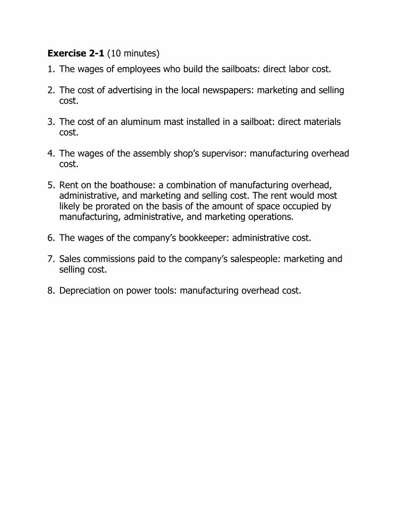
Exercise 2-1 (10 minutes)
1. The wages of employees who build the sailboats: direct labor cost. 2. The cost of advertising in the local newspapers: marketing and selling
cost. 3. The cost of an aluminum mast installed in a sailboat: direct materials
cost. 4. The wages of the assembly shop’s supervisor: manufacturing overhead
cost. 5. Rent on the boathouse: a combination of manufacturing overhead,
administrative, and marketing and selling cost. The rent would most likely be prorated on the basis of the amount of space occupied by manufacturing, administrative, and marketing operations.
6. The wages of the company’s bookkeeper: administrative cost. 7. Sales commissions paid to the company’s salespeople: marketing and
selling cost. 8. Depreciation on power tools: manufacturing overhead cost.
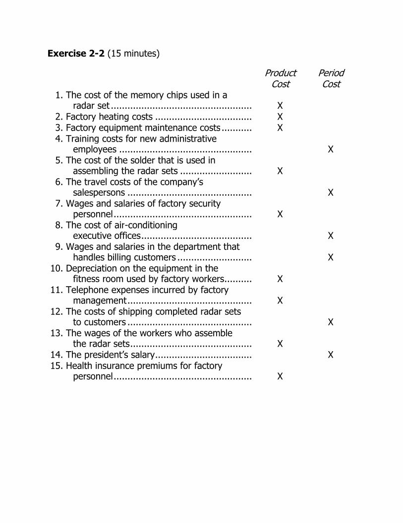
Exercise 2-2 (15 minutes)
Product Cost
Period Cost
1. The cost of the memory chips used in a radar set ................................................... X
2. Factory heating costs ................................... X 3. Factory equipment maintenance costs ........... X 4. Training costs for new administrative
employees ................................................ X 5. The cost of the solder that is used in
assembling the radar sets .......................... X 6. The travel costs of the company’s
salespersons ............................................. X 7. Wages and salaries of factory security
personnel .................................................. X 8. The cost of air-conditioning
executive offices ........................................ X 9. Wages and salaries in the department that
handles billing customers ........................... X 10. Depreciation on the equipment in the
fitness room used by factory workers .......... X 11. Telephone expenses incurred by factory
management ............................................. X 12. The costs of shipping completed radar sets
to customers ............................................. X 13. The wages of the workers who assemble
the radar sets ............................................ X 14. The president’s salary ................................... X 15. Health insurance premiums for factory
personnel .................................................. X
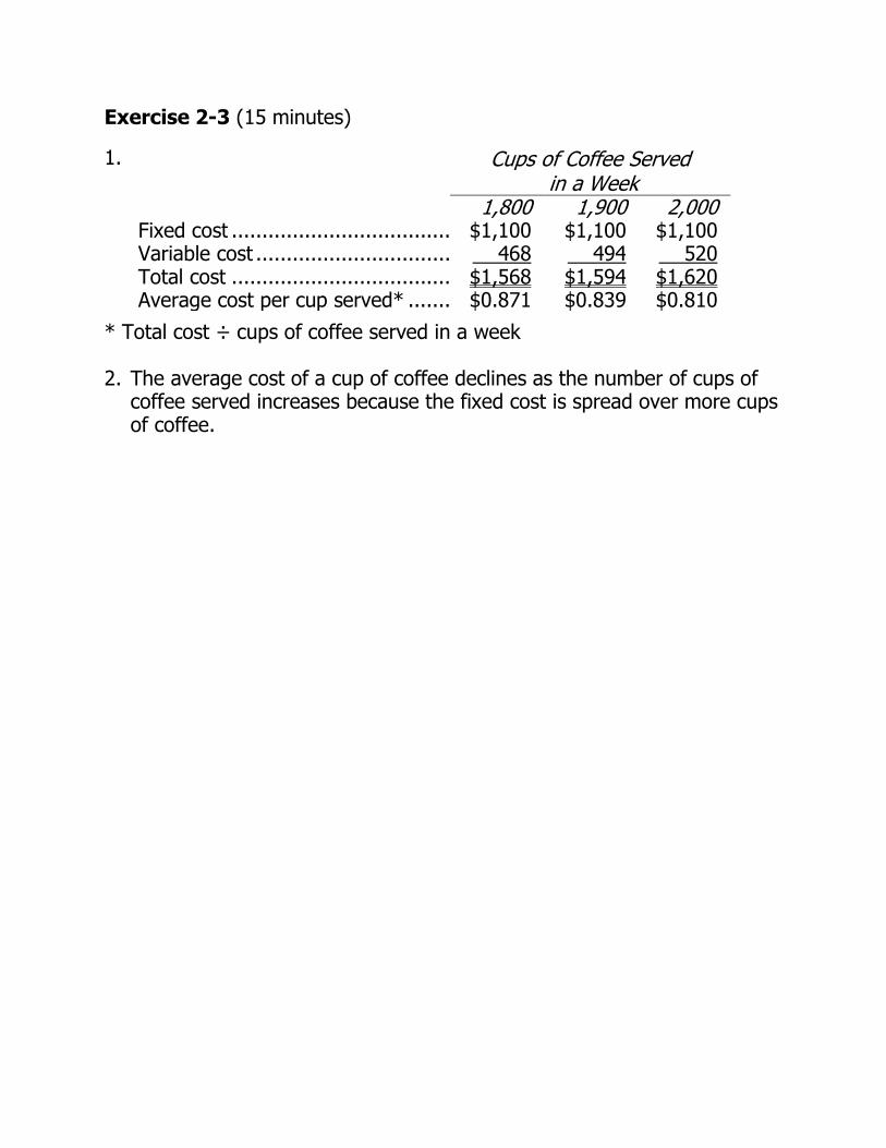
Exercise 2-3 (15 minutes)
1. Cups of Coffee Served in a Week
1,800 1,900 2,000 Fixed cost ................................................................$1,100 $1,100 $1,100 Variable cost ................................ 468 494 520 Total cost ................................................................$1,568 $1,594 $1,620 Average cost per cup served* ................................$0.871 $0.839 $0.810
* Total cost ÷ cups of coffee served in a week 2. The average cost of a cup of coffee declines as the number of cups of
coffee served increases because the fixed cost is spread over more cups of coffee.

Exercise 2-4 (20 minutes)
1.
Occupancy-
Days Electrical
Costs High activity level (August) .. 3,608 $8,111 Low activity level (October) .. 186 1,712 Change ............................... 3,422 $6,399
Variable cost = Change in cost ÷ Change in activity = $6,399 ÷ 3,422 occupancy-days = $1.87 per occupancy-day
Total cost (August) .................................................... $8,111
Variable cost element
($1.87 per occupancy-day × 3,608 occupancy-days) 6,747 Fixed cost element .................................................... $1,364
2. Electrical costs may reflect seasonal factors other than just the variation
in occupancy days. For example, common areas such as the reception area must be lighted for longer periods during the winter. This will result in seasonal effects on the fixed electrical costs.
Additionally, fixed costs will be affected by how many days are in a month. In other words, costs like the costs of lighting common areas are variable with respect to the number of days in the month, but are fixed with respect to how many rooms are occupied during the month.
Other, less systematic, factors may also affect electrical costs such as the frugality of individual guests. Some guests will turn off lights when they leave a room. Others will not.

Exercise 2-5 (15 minutes)
1. Traditional income statement
Redhawk, Inc. Traditional Income Statement
Sales ($15 per unit × 10,000 units) .................... $150,000 Cost of goods sold
($12,000 + $90,000 – $22,000) ....................... 80,000 Gross margin ..................................................... 70,000 Selling and administrative expenses:
Selling expenses (($2 per unit × 10,000 units) + $20,000) ...... 40,000
Administrative expenses (($1 per unit × 10,000 units) + $15,000) ...... 25,000 65,000
Net operating income ........................................ $ 5,000 2. Contribution format income statement
Redhawk, Inc. Contribution Format Income Statement
Sales ................................................................ $150,000 Variable expenses:
Cost of goods sold ($12,000 + $90,000 – $22,000) .................... $80,000
Selling expenses ($2 per unit × 10,000 units) ... 20,000 Administrative expenses
($1 per unit × 10,000 units) ......................... 10,000 110,000 Contribution margin ........................................... 40,000 Fixed expenses:
Selling expenses ............................................. 20,000 Administrative expenses .................................. 15,000 35,000
Net operating income ........................................ $ 5,000

Exercise 2-6 (15 minutes)
Direct Indirect Cost Cost Object Cost Cost
1. The salary of the head chef
The hotel’s restaurant X
2. The salary of the head chef
A particular restaurant customer
X
3. Room cleaning supplies A particular hotel guest X 4. Flowers for the
reception desk A particular hotel guest X
5. The wages of the doorman
A particular hotel guest X
6. Room cleaning supplies The housecleaning department
X
7. Fire insurance on the hotel building
The hotel’s gym X
8. Towels used in the gym The hotel’s gym X
Note: The room cleaning supplies would most likely be considered an indirect cost of a particular hotel guest because it would not be practical to keep track of exactly how much of each cleaning supply was used in the guest’s room.
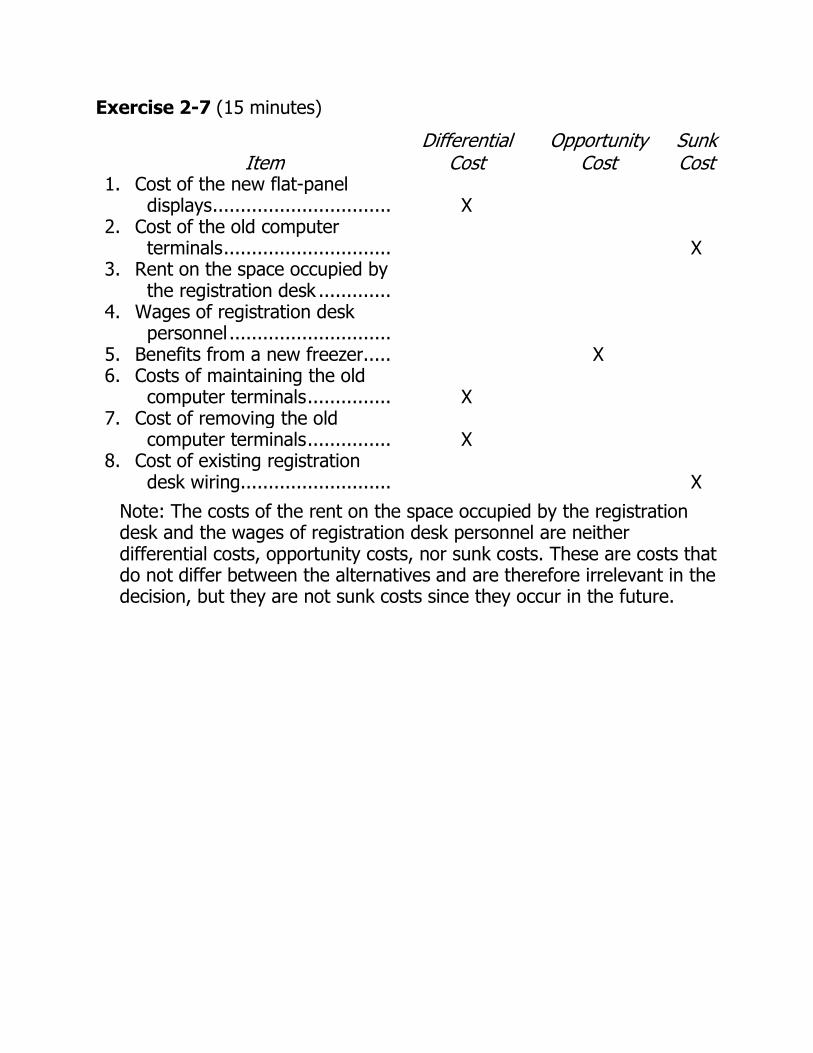
Exercise 2-7 (15 minutes)
Differential Opportunity Sunk Item Cost Cost Cost
1. Cost of the new flat-panel displays ................................ X
2. Cost of the old computer terminals .............................. X
3. Rent on the space occupied by the registration desk .............
4. Wages of registration desk personnel .............................
5. Benefits from a new freezer..... X 6. Costs of maintaining the old
computer terminals ............... X 7. Cost of removing the old
computer terminals ............... X 8. Cost of existing registration
desk wiring........................... X
Note: The costs of the rent on the space occupied by the registration desk and the wages of registration desk personnel are neither differential costs, opportunity costs, nor sunk costs. These are costs that do not differ between the alternatives and are therefore irrelevant in the decision, but they are not sunk costs since they occur in the future.
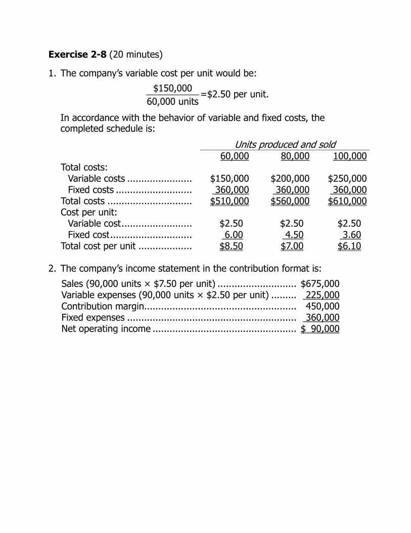
Exercise 2-8 (20 minutes)
1. The company’s variable cost per unit would be:
$150,000
=$2.50 per unit.60,000 units
In accordance with the behavior of variable and fixed costs, the completed schedule is:
Units produced and sold 60,000 80,000 100,000 Total costs:
Variable costs ....................... $150,000 $200,000 $250,000 Fixed costs ........................... 360,000 360,000 360,000
Total costs .............................. $510,000 $560,000 $610,000 Cost per unit:
Variable cost ......................... $2.50 $2.50 $2.50 Fixed cost ............................. 6.00 4.50 3.60
Total cost per unit ................... $8.50 $7.00 $6.10
2. The company’s income statement in the contribution format is:
Sales (90,000 units × $7.50 per unit) ............................ $675,000 Variable expenses (90,000 units × $2.50 per unit) ......... 225,000 Contribution margin...................................................... 450,000 Fixed expenses ............................................................ 360,000 Net operating income ................................................... $ 90,000

Problem 2-14 (45 minutes)
1. House Of Organs, Inc. Traditional Income Statement For the Month Ended November 30
Sales (60 organs × $2,500 per organ) ................ $150,000
Cost of goods sold
(60 organs × $1,500 per organ) ...................... 90,000 Gross margin .................................................... 60,000 Selling and administrative expenses: Selling expenses: Advertising .................................................. $ 950
Delivery of organs
(60 organs × $60 per organ) ...................... 3,600
Sales salaries and commissions
[$4,800 + (4% × $150,000)] ..................... 10,800 Utilities ........................................................ 650 Depreciation of sales facilities ....................... 5,000 Total selling expenses ..................................... 21,000 Administrative expenses: Executive salaries ......................................... 13,500 Depreciation of office equipment ................... 900
Clerical
[$2,500 + (60 organs × $40 per organ)] .... 4,900 Insurance .................................................... 700 Total administrative expenses .......................... 20,000 Total selling and administrative expenses ............ 41,000 Net operating income ........................................ $ 19,000

Problem 2-14 (continued)
2. House Of Organs, Inc. Contribution Format Income Statement For the Month Ended November 30
Total Per Unit Sales (60 organs × $2,500 per organ) ................ $150,000 $2,500 Variable expenses:
Cost of goods sold
(60 organs × $1,500 per organ) .................... 90,000 1,500
Delivery of organs
(60 organs × $60 per organ) ........................ 3,600 60 Sales commissions (4% × $150,000) ............... 6,000 100 Clerical (60 organs × $40 per organ) ............... 2,400 40 Total variable expenses ................................. 102,000 1,700 Contribution margin ........................................... 48,000 $ 800 Fixed expenses: Advertising ..................................................... 950 Sales salaries .................................................. 4,800 Utilities ........................................................... 650 Depreciation of sales facilities .......................... 5,000 Executive salaries ........................................... 13,500 Depreciation of office equipment ..................... 900 Clerical ........................................................... 2,500 Insurance ....................................................... 700 Total fixed expenses .......................................... 29,000 Net operating income ........................................ $ 19,000
3. Fixed costs remain constant in total but vary on a per unit basis with
changes in the activity level. For example, as the activity level increases, fixed costs decrease on a per unit basis. Showing fixed costs on a per unit basis on the income statement make them appear to be variable costs. That is, management might be misled into thinking that the per unit fixed costs would be the same regardless of how many organs were sold during the month. For this reason, fixed costs should be shown only in totals on a contribution-type income statement.
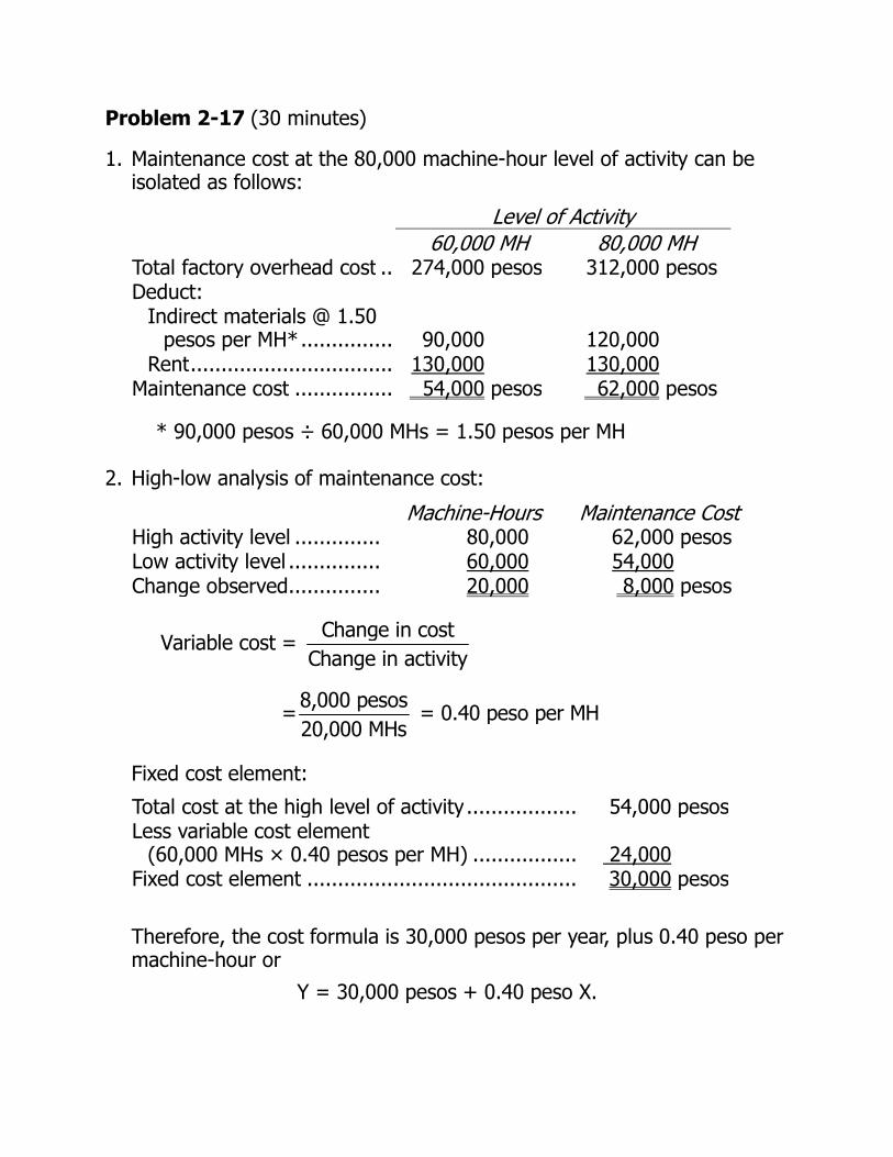
Problem 2-17 (30 minutes)
1. Maintenance cost at the 80,000 machine-hour level of activity can be isolated as follows:
Level of Activity 60,000 MH 80,000 MH Total factory overhead cost .. 274,000 pesos 312,000 pesos Deduct:
Indirect materials @ 1.50 pesos per MH* ............... 90,000 120,000
Rent ................................. 130,000 130,000 Maintenance cost ................ 54,000 pesos 62,000 pesos
* 90,000 pesos ÷ 60,000 MHs = 1.50 pesos per MH 2. High-low analysis of maintenance cost:
Machine-Hours Maintenance Cost High activity level .............. 80,000 62,000 pesos Low activity level ............... 60,000 54,000 Change observed ............... 20,000 8,000 pesos
Change in costVariable cost =
Change in activity
8,000 pesos= = 0.40 peso per MH
20,000 MHs
Fixed cost element:
Total cost at the high level of activity .................. 54,000 pesos Less variable cost element
(60,000 MHs × 0.40 pesos per MH) ................. 24,000
Fixed cost element ............................................ 30,000 pesos
Therefore, the cost formula is 30,000 pesos per year, plus 0.40 peso per
machine-hour or
Y = 30,000 pesos + 0.40 peso X.

Problem 2-17 (continued)
3. Total factory overhead cost at 65,000 machine-hours is:
Indirect materials (65,000 MHs × 1.50 pesos per MH) ....................... 97,500 pesos
Rent ................................................ 130,000 Maintenance:
Variable cost element (65,000 MHs
× 0.40 peso per MH) ................... 26,000 pesos Fixed cost element ......................... 30,000 56,000 Total factory overhead cost ............... 283,500 pesos
Problem 2-21 (45 minutes)
1. Maintenance cost at the 70,000 machine-hour level of activity can be isolated as follows:
Level of Activity
40,000 MH 70,000 MH Total factory overhead cost ............. $170,200 $241,600 Deduct:
Utilities cost @ $1.30 per MH* ...... 52,000 91,000 Supervisory salaries ..................... 60,000 60,000
Maintenance cost ........................... $ 58,200 $ 90,600
*$52,000 ÷ 40,000 MHs = $1.30 per MH 2. High-low analysis of maintenance cost:
Machine-
Hours Maintenance
Cost High activity level .............. 70,000 $90,600 Low activity level ............... 40,000 58,200 Change ............................. 30,000 $32,400
Variable cost per unit of activity:
Change in cost $32,400
= =$1.08 per MHChange in activity 30,000 MHs
Total fixed cost:

Total maintenance cost at the low activity level ............ $58,200 Less the variable cost element
(40,000 MHs × $1.08 per MH) .................................. 43,200 Fixed cost element ..................................................... $15,000
Therefore, the cost formula is $15,000 per month plus $1.08 per machine-hour or:
Y = $15,000 + $1.08X
Problem 2-21 (continued)
3.
Variable Rate per
Machine-Hour Fixed Cost Maintenance cost .............. $1.08 $15,000 Utilities cost ...................... 1.30 Supervisory salaries cost .... 60,000 Totals ............................... $2.38 $75,000
Thus, the cost formula is: Y = $75,000 + $2.38X. 4. Total overhead cost at an activity level of 45,000 machine-hours:
Fixed costs .......................................................... $ 75,000 Variable costs: $2.38 per MH × 45,000 MHs.......... 107,100 Total overhead costs ............................................ $182,100
Problem 2-23 (45 minutes)
1. High-low method:
Units Sold
Shipping Expense
High activity level .............. 25,000 $232,000 Low activity level ............... 16,000 160,000 Change ............................. 9,000 $72,000
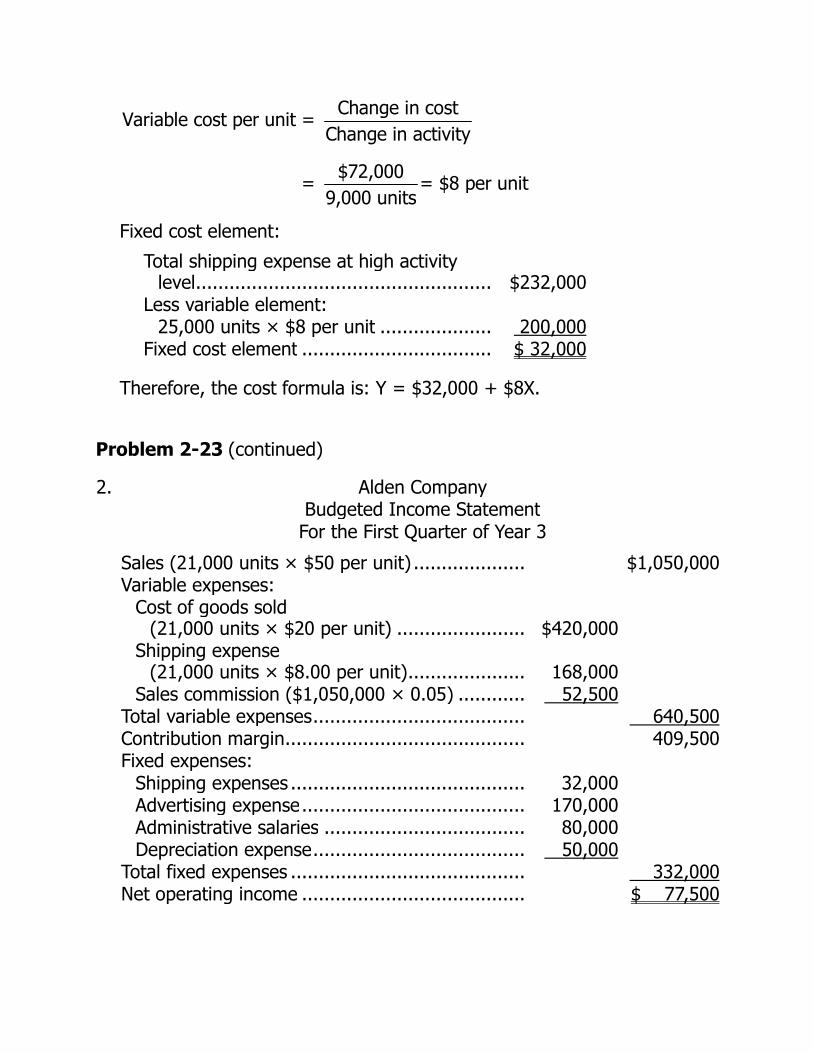
Change in costVariable cost per unit =
Change in activity
$72,000= = $8 per unit
9,000 units
Fixed cost element:
Total shipping expense at high activity
level ..................................................... $232,000 Less variable element: 25,000 units × $8 per unit .................... 200,000 Fixed cost element .................................. $ 32,000
Therefore, the cost formula is: Y = $32,000 + $8X.
Problem 2-23 (continued)
2. Alden Company Budgeted Income Statement For the First Quarter of Year 3
Sales (21,000 units × $50 per unit) .................... $1,050,000 Variable expenses:
Cost of goods sold
(21,000 units × $20 per unit) ....................... $420,000
Shipping expense
(21,000 units × $8.00 per unit) ..................... 168,000 Sales commission ($1,050,000 × 0.05) ............ 52,500 Total variable expenses ...................................... 640,500 Contribution margin ........................................... 409,500 Fixed expenses: Shipping expenses .......................................... 32,000 Advertising expense ........................................ 170,000 Administrative salaries .................................... 80,000 Depreciation expense ...................................... 50,000 Total fixed expenses .......................................... 332,000 Net operating income ........................................ $ 77,500
© The McGraw-Hill Companies, Inc., 2012. All rights reserved.
Solutions Manual, Chapter 3 67
Chapter 3 Job-Order Costing
Solutions to Questions
3-1 By definition, manufacturing overhead consists of costs that cannot be practically traced to jobs. Therefore, if these costs are to be assigned to jobs, they must be allocated rather than traced.
3-2 The first step is to estimate the total amount of the allocation base (the denominator) that will be required for next period’s estimated level of production. The second step is to estimate the total fixed manufacturing overhead cost for the coming period and the variable manufacturing overhead cost per unit of the allocation base. The third step is to use the cost formula Y = a + bX to estimate the total manufacturing overhead cost (the numerator) for the coming period. The fourth step is to compute the predetermined overhead rate.
3-3 The job cost sheet is used to record all costs that are assigned to a particular job. These costs include direct materials costs traced to the job, direct labor costs traced to the job, and manufacturing overhead costs applied to the job. When a job is completed, the job cost sheet is used to compute the unit product cost.
3-4 A sales order is issued after an agreement has been reached with a customer on quantities, prices, and shipment dates for goods. The sales order forms the basis for the production order. The production order specifies what is to be produced and forms the basis for the job cost sheet. The job cost sheet, in turn, is used to summarize the various production costs incurred to complete the job. These costs are entered on the job cost sheet from materials requisition forms, direct labor time tickets, and by applying overhead.
3-5 Some production costs such as a factory manager’s salary cannot be traced to a particular product or job, but rather are incurred as a result
of overall production activities. In addition, some production costs such as indirect materials cannot be easily traced to jobs. If these costs are to be assigned to products, they must be allocated to the products.
3-6 If actual manufacturing overhead cost is applied to jobs, the company must wait until the end of the accounting period to apply overhead and to cost jobs. If the company computes actual overhead rates more frequently to get around this problem, the rates may fluctuate widely due to seasonal factors or variations in output. For this reason, most companies use predetermined overhead rates to apply manufacturing overhead costs to jobs.
3-7 The measure of activity used as the allocation base should drive the overhead cost; that is, the allocation base should cause the overhead cost. If the allocation base does not really cause the overhead, then costs will be incorrectly attributed to products and jobs and product costs will be distorted.
3-8 Assigning manufacturing overhead costs to jobs does not ensure a profit. The units produced may not be sold and if they are sold, they may not be sold at prices sufficient to cover all costs. It is a myth that assigning costs to products or jobs ensures that those costs will be recovered. Costs are recovered only by selling to customers—not by allocating costs.
3-9 The Manufacturing Overhead account is credited when overhead cost is applied to Work in Process. Generally, the amount of overhead applied will not be the same as the amount of actual cost incurred because the predetermined overhead rate is based on estimates.
3-10 Underapplied overhead occurs when the actual overhead cost exceeds the amount of

© The McGraw-Hill Companies, Inc., 2012. All rights reserved.
68 Managerial Accounting, 14th edition
overhead cost applied to Work in Process inventory during the period. Overapplied overhead occurs when the actual overhead cost is less than the amount of overhead cost applied to Work in Process inventory during the period. Underapplied or overapplied overhead is disposed of by either closing out the amount to Cost of Goods Sold or by allocating the amount among Cost of Goods Sold and ending inventories in proportion to the applied overhead in each account. The adjustment for underapplied overhead increases Cost of Goods Sold (and inventories) whereas the adjustment for overapplied overhead decreases Cost of Goods Sold (and inventories).
3-11 Manufacturing overhead may be underapplied for several reasons. Control over overhead spending may be poor. Or, some of the overhead may be fixed and the actual amount of the allocation base may be less than estimated at the beginning of the period. In this situation, the amount of overhead applied to inventory will be less than the actual overhead cost incurred.
3-12 Underapplied overhead implies that not enough overhead was assigned to jobs during the
period and therefore cost of goods sold was understated. Therefore, underapplied overhead is added to cost of goods sold. On the other hand, overapplied overhead is deducted from cost of goods sold.
3-13 A plantwide overhead rate is a single overhead rate used throughout a plant. In a multiple overhead rate system, each production department may have its own predetermine overhead rate and its own allocation base. Some companies use multiple overhead rates rather than plantwide rates to more appropriately allocate overhead costs among products. Multiple overhead rates should be used, for example, in situations where one department is machine intensive and another department is labor intensive.
3-14 When automated equipment replaces direct labor, overhead increases and direct labor decreases. This results in an increase in the predetermined overhead rate—particularly if it is based on direct labor.

© The McGraw-Hill Companies, Inc., 2012. All rights reserved.
Solutions Manual, Chapter 3 69
Exercise 3-1 (10 minutes)
The estimated total manufacturing overhead cost is computed as follows:
Y = $466,000 + ($3.00 per DLH)(40,000 DLHs)
Estimated fixed manufacturing overhead .................. $466,000
Estimated variable manufacturing overhead:
$3.00 per DLH × 40,000 DLHs ............................... 120,000 Estimated total manufacturing overhead cost ............ $586,000
The predetermined overhead rate is computed as follows:
Estimated total manufacturing overhead ....... $586,000 ÷ Estimated total direct labor hours (DLHs) .. 40,000 DLHs = Predetermined overhead rate .................... $14.65 per DLH

© The McGraw-Hill Companies, Inc., 2012. All rights reserved.
70 Managerial Accounting, 14th edition
Exercise 3-2 (10 minutes)
Actual direct labor-hours .......................... 12,600 × Predetermined overhead rate ................ $23.10 = Manufacturing overhead applied ........... $291,060

© The McGraw-Hill Companies, Inc., 2012. All rights reserved.
Solutions Manual, Chapter 3 71
Exercise 3-3 (10 minutes)
1. Total direct labor-hours required for Job A-200:
Direct labor cost ............................... $120 ÷ Direct labor wage rate per hour ..... $12 = Total direct labor hours ................. 10
Total manufacturing cost assigned to Job A-200:
Direct materials ................................ $200 Direct labor ...................................... 120 Manufacturing overhead applied
($18 per DLH × 10 DLHs) .............. 180 Total manufacturing cost .................. $500
2. Unit product cost for Job A-200:
Total manufacturing cost ................. $500 ÷ Number of units in the job ........... 50 = Unit product cost ......................... $10
© The McGraw-Hill Companies, Inc., 2012. All rights reserved.
72 Managerial Accounting, 14th edition
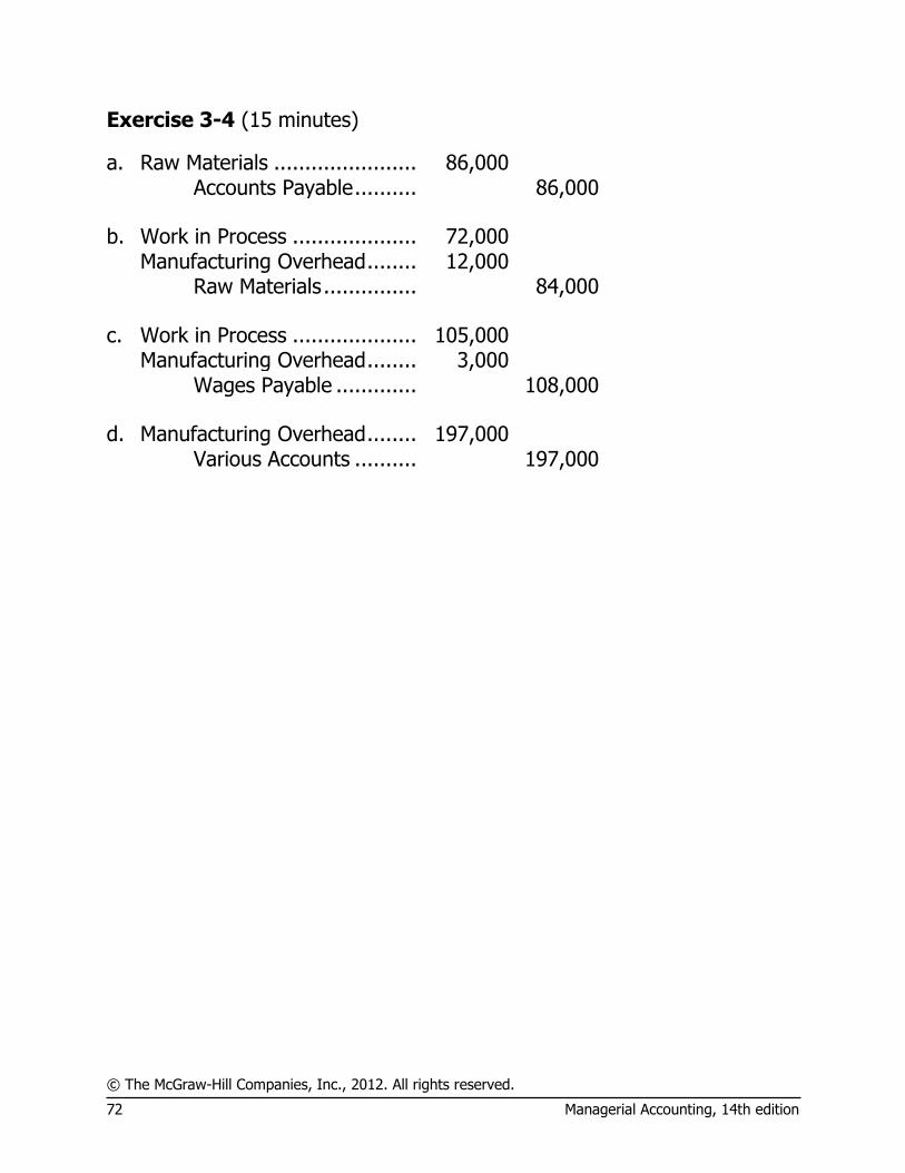
Exercise 3-4 (15 minutes)
a. Raw Materials ....................... 86,000 Accounts Payable .......... 86,000
b. Work in Process .................... 72,000 Manufacturing Overhead ........ 12,000 Raw Materials ............... 84,000
c. Work in Process .................... 105,000 Manufacturing Overhead ........ 3,000 Wages Payable ............. 108,000 d. Manufacturing Overhead ........ 197,000 Various Accounts .......... 197,000
© The McGraw-Hill Companies, Inc., 2012. All rights reserved.
Solutions Manual, Chapter 3 73
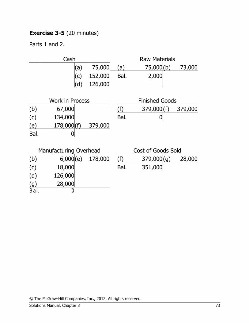
Exercise 3-5 (20 minutes)
Parts 1 and 2.
Cash Raw Materials
(a) 75,000 (a) 75,000 (b) 73,000
(c) 152,000 Bal. 2,000
(d) 126,000
Work in Process Finished Goods
(b) 67,000 (f) 379,000 (f) 379,000
(c) 134,000 Bal. 0
(e) 178,000 (f) 379,000
Bal. 0
Manufacturing Overhead Cost of Goods Sold
(b) 6,000 (e) 178,000 (f) 379,000 (g) 28,000
(c) 18,000 Bal. 351,000
(d) 126,000
(g) 28,000 Bal. 0
© The McGraw-Hill Companies, Inc., 2012. All rights reserved.
74 Managerial Accounting, 14th edition
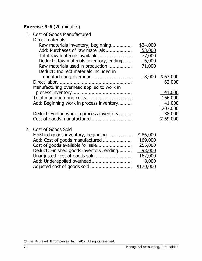
Exercise 3-6 (20 minutes)
1. Cost of Goods Manufactured Direct materials: Raw materials inventory, beginning............... $24,000 Add: Purchases of raw materials ................... 53,000 Total raw materials available ........................ 77,000 Deduct: Raw materials inventory, ending ...... 6,000 Raw materials used in production ................. 71,000 Deduct: Indirect materials included in
manufacturing overhead ............................. 8,000 $ 63,000 Direct labor ...................................................... 62,000 Manufacturing overhead applied to work in
process inventory ........................................... 41,000 Total manufacturing costs ................................. 166,000 Add: Beginning work in process inventory.......... 41,000 207,000 Deduct: Ending work in process inventory ......... 38,000 Cost of goods manufactured ............................. $169,000 2. Cost of Goods Sold Finished goods inventory, beginning .................. $ 86,000 Add: Cost of goods manufactured ..................... 169,000 Cost of goods available for sale ......................... 255,000 Deduct: Finished goods inventory, ending.......... 93,000 Unadjusted cost of goods sold .......................... 162,000 Add: Underapplied overhead ............................. 8,000 Adjusted cost of goods sold .............................. $170,000

© The McGraw-Hill Companies, Inc., 2012. All rights reserved.
Solutions Manual, Chapter 3 75
Exercise 3-7 (10 minutes)
1. Actual direct labor-hours ......................... 8,250 × Predetermined overhead rate ............... $21.40 = Manufacturing overhead applied ........... $176,550 Less: Manufacturing overhead incurred .... 172,500 Manufacturing overhead overapplied ........ $ 4,050
2. Because manufacturing overhead is overapplied, the cost of goods sold
would decrease by $4,050 and the gross margin would increase by $4,050.

© The McGraw-Hill Companies, Inc., 2012. All rights reserved.
76 Managerial Accounting, 14th edition
Exercise 3-8 (30 minutes)
1. Cost of Goods Manufactured Direct materials: Raw materials inventory, beginning............... $ 8,000 Add: Purchases of raw materials ................... 132,000 Total raw materials available ........................ 140,000 Deduct: Raw materials inventory, ending ...... 10,000 Raw materials used in production ................. 130,000 Direct labor ...................................................... 90,000 Manufacturing overhead applied to work in
process inventory ........................................... 210,000 Total manufacturing costs ................................. 430,000 Add: Beginning work in process inventory.......... 5,000 435,000 Deduct: Ending work in process inventory ......... 20,000 Cost of goods manufactured ............................. $415,000 2. Cost of Goods Sold Finished goods inventory, beginning .................. $ 70,000 Add: Cost of goods manufactured ..................... 415,000 Cost of goods available for sale ......................... 485,000 Deduct: Finished goods inventory, ending.......... 25,000 Unadjusted cost of goods sold .......................... 460,000 Add: Underapplied overhead ............................. 10,000 Adjusted cost of goods sold .............................. $470,000
3. Eccles Company
Income Statement
Sales .............................................................. $643,000 Cost of goods sold ($460,000 + $10,000) ......... 470,000 Gross margin ................................................... 173,000 Selling and administrative expenses:
Selling expenses ........................................... $100,000 Administrative expense ................................. 43,000 143,000
Net operating income ...................................... $ 30,000
© The McGraw-Hill Companies, Inc., 2012. All rights reserved.
Solutions Manual, Chapter 3 77
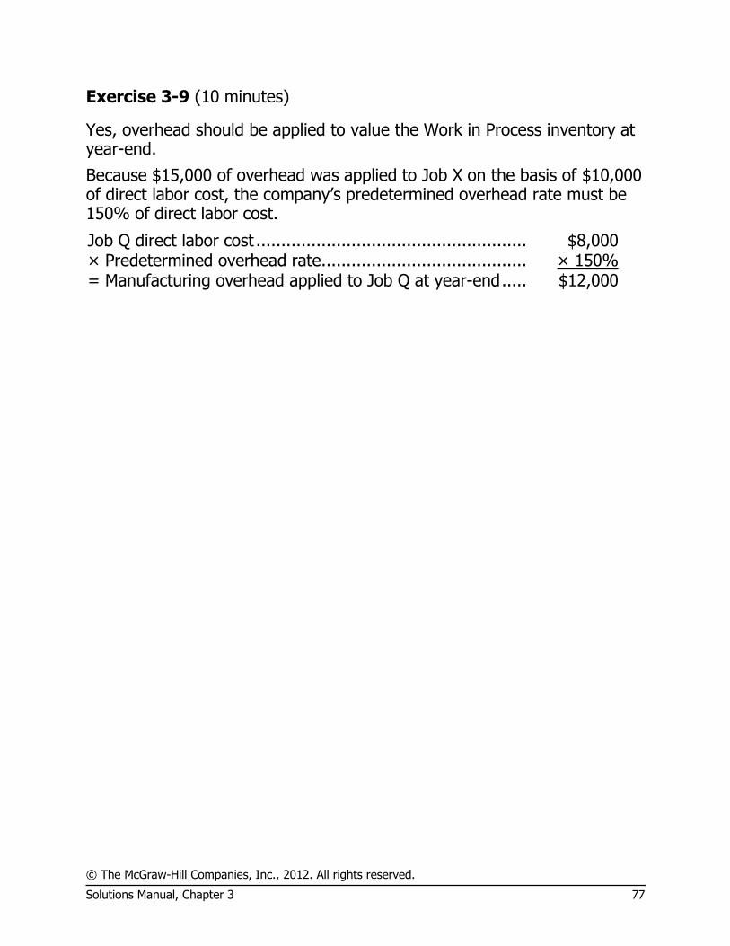
Exercise 3-9 (10 minutes)
Yes, overhead should be applied to value the Work in Process inventory at year-end.
Because $15,000 of overhead was applied to Job X on the basis of $10,000 of direct labor cost, the company’s predetermined overhead rate must be 150% of direct labor cost.
Job Q direct labor cost ...................................................... $8,000 × Predetermined overhead rate ......................................... × 150% = Manufacturing overhead applied to Job Q at year-end ..... $12,000
© The McGraw-Hill Companies, Inc., 2012. All rights reserved.
78 Managerial Accounting, 14th edition
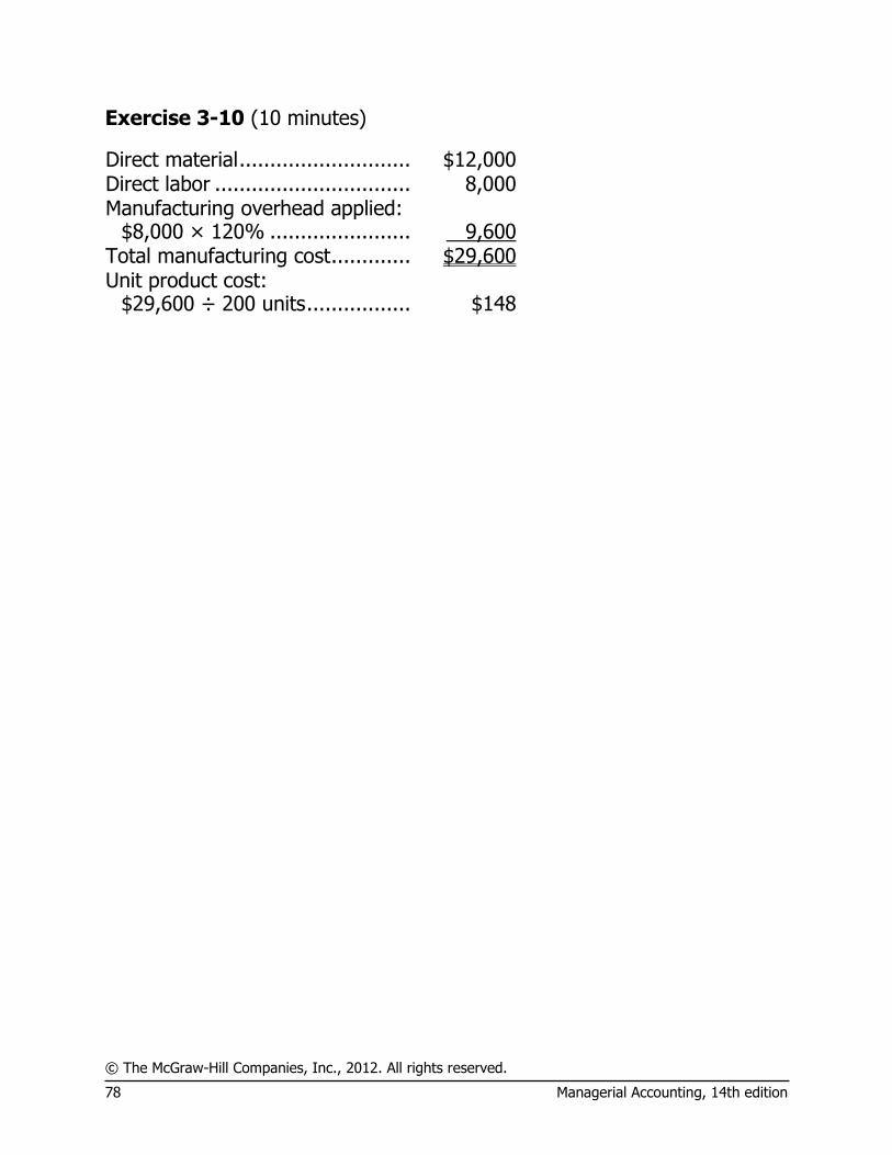
Exercise 3-10 (10 minutes)
Direct material ............................ $12,000 Direct labor ................................ 8,000 Manufacturing overhead applied:
$8,000 × 120% ....................... 9,600 Total manufacturing cost ............. $29,600 Unit product cost:
$29,600 ÷ 200 units ................. $148

© The McGraw-Hill Companies, Inc., 2012. All rights reserved.
Solutions Manual, Chapter 3 79
Exercise 3-11 (30 minutes)
1. a. Raw Materials Inventory ......................... 210,000 Accounts Payable ................................ 210,000
b. Work in Process ..................................... 152,000 Manufacturing Overhead ........................ 38,000 Raw Materials Inventory ...................... 190,000
c. Work in Process ..................................... 49,000 Manufacturing Overhead ........................ 21,000 Salaries and Wages Payable ................. 70,000
d. Manufacturing Overhead ........................ 105,000 Accumulated Depreciation .................... 105,000
e. Manufacturing Overhead ........................ 130,000 Accounts Payable ................................ 130,000
f. Work in Process ..................................... 300,000 Manufacturing Overhead ...................... 300,000 75,000 machine-hours $4 per machine-hour = $300,000.
g. Finished Goods ...................................... 510,000 Work in Process ................................... 510,000
h. Cost of Goods Sold ................................. 450,000 Finished Goods .................................... 450,000 Accounts Receivable ............................... 675,000 Sales .................................................. 675,000 $450,000 × 1.5 = $675,000. 2. Manufacturing Overhead Work in Process
(b) 38,000 (f) 300,000 Bal. 35,000 (g) 510,000
(c) 21,000 (b) 152,000
(d) 105,000 (c) 49,000
(e) 130,000 (f) 300,000
6,000 Bal. 26,000
(Overapplied overhead)
© The McGraw-Hill Companies, Inc., 2012. All rights reserved.
80 Managerial Accounting, 14th edition
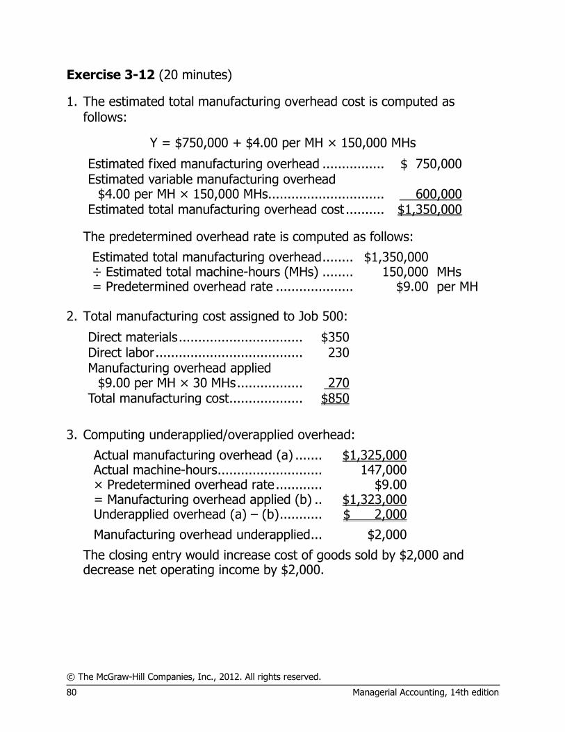
Exercise 3-12 (20 minutes)
1. The estimated total manufacturing overhead cost is computed as follows:
Y = $750,000 + $4.00 per MH × 150,000 MHs
Estimated fixed manufacturing overhead ................ $ 750,000 Estimated variable manufacturing overhead
$4.00 per MH × 150,000 MHs .............................. 600,000 Estimated total manufacturing overhead cost .......... $1,350,000
The predetermined overhead rate is computed as follows:
Estimated total manufacturing overhead ........ $1,350,000 ÷ Estimated total machine-hours (MHs) ........ 150,000 MHs = Predetermined overhead rate .................... $9.00 per MH
2. Total manufacturing cost assigned to Job 500:
Direct materials ................................ $350 Direct labor ...................................... 230 Manufacturing overhead applied
$9.00 per MH × 30 MHs ................. 270 Total manufacturing cost ................... $850
3. Computing underapplied/overapplied overhead:
Actual manufacturing overhead (a) ....... $1,325,000 Actual machine-hours ........................... 147,000 × Predetermined overhead rate ............ $9.00 = Manufacturing overhead applied (b) .. $1,323,000 Underapplied overhead (a) – (b) ........... $ 2,000
Manufacturing overhead underapplied ... $2,000
The closing entry would increase cost of goods sold by $2,000 and decrease net operating income by $2,000.

© The McGraw-Hill Companies, Inc., 2012. All rights reserved.
Solutions Manual, Chapter 3 81
Exercise 3-13 (15 minutes)
1. Actual manufacturing overhead costs .............. $ 48,000
Manufacturing overhead applied:
10,000 MH × $5 per MH .............................. 50,000 Overapplied overhead cost .............................. $ 2,000 2. Direct materials: Raw materials inventory, beginning .............. $ 8,000 Add: Purchases of raw materials ................... 32,000 Raw materials available for use .................... 40,000 Deduct: Raw materials inventory, ending ...... 7,000 Raw materials used in production ................. $ 33,000 Direct labor .................................................... 40,000
Manufacturing overhead cost applied to work
in process ................................................... 50,000 Total manufacturing cost ................................ 123,000 Add: Work in process, beginning ..................... 6,000 129,000 Deduct: Work in process, ending ..................... 7,500 Cost of goods manufactured ........................... $121,500
© The McGraw-Hill Companies, Inc., 2012. All rights reserved.
82 Managerial Accounting, 14th edition
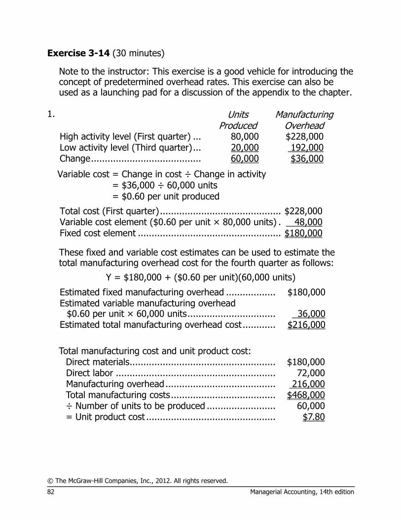
Exercise 3-14 (30 minutes)
Note to the instructor: This exercise is a good vehicle for introducing the concept of predetermined overhead rates. This exercise can also be used as a launching pad for a discussion of the appendix to the chapter.
1.
Units
Produced Manufacturing
Overhead High activity level (First quarter) ... 80,000 $228,000 Low activity level (Third quarter) ... 20,000 192,000 Change ........................................ 60,000 $36,000
Variable cost = Change in cost ÷ Change in activity = $36,000 ÷ 60,000 units = $0.60 per unit produced
Total cost (First quarter) ............................................ $228,000 Variable cost element ($0.60 per unit × 80,000 units) . 48,000 Fixed cost element .................................................... $180,000
These fixed and variable cost estimates can be used to estimate the total manufacturing overhead cost for the fourth quarter as follows:
Y = $180,000 + ($0.60 per unit)(60,000 units)
Estimated fixed manufacturing overhead .................. $180,000
Estimated variable manufacturing overhead
$0.60 per unit × 60,000 units ................................ 36,000 Estimated total manufacturing overhead cost ............ $216,000
Total manufacturing cost and unit product cost:
Direct materials ..................................................... $180,000 Direct labor .......................................................... 72,000 Manufacturing overhead ........................................ 216,000 Total manufacturing costs ...................................... $468,000 ÷ Number of units to be produced ......................... 60,000 = Unit product cost ............................................... $7.80
© The McGraw-Hill Companies, Inc., 2012. All rights reserved.
Solutions Manual, Chapter 3 83
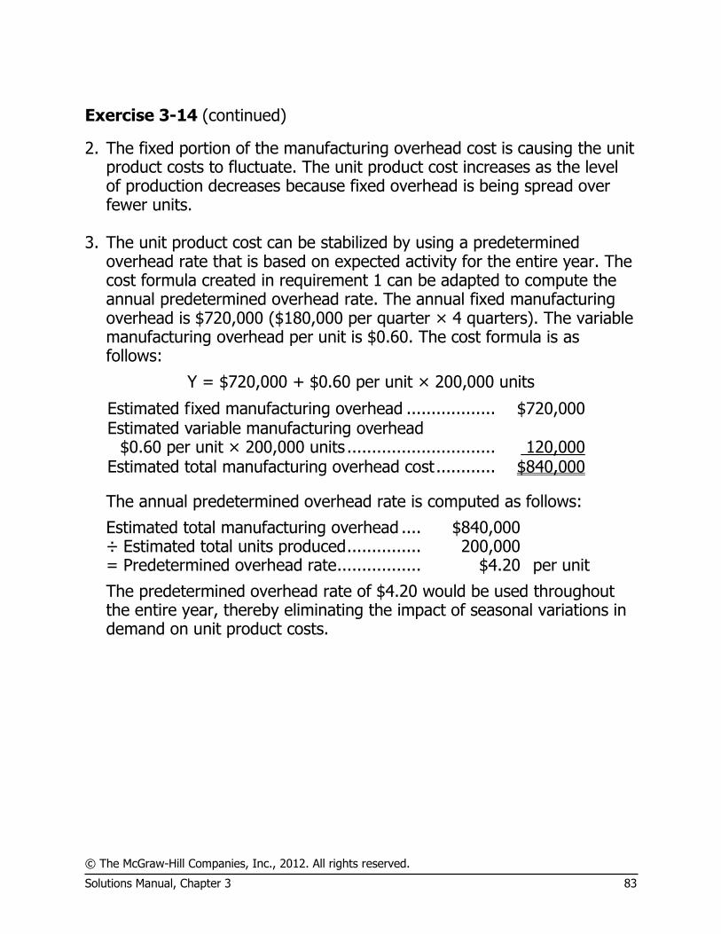
Exercise 3-14 (continued)
2. The fixed portion of the manufacturing overhead cost is causing the unit product costs to fluctuate. The unit product cost increases as the level of production decreases because fixed overhead is being spread over fewer units.
3. The unit product cost can be stabilized by using a predetermined
overhead rate that is based on expected activity for the entire year. The cost formula created in requirement 1 can be adapted to compute the annual predetermined overhead rate. The annual fixed manufacturing overhead is $720,000 ($180,000 per quarter × 4 quarters). The variable manufacturing overhead per unit is $0.60. The cost formula is as follows:
Y = $720,000 + $0.60 per unit × 200,000 units
Estimated fixed manufacturing overhead .................. $720,000
Estimated variable manufacturing overhead
$0.60 per unit × 200,000 units .............................. 120,000 Estimated total manufacturing overhead cost ............ $840,000
The annual predetermined overhead rate is computed as follows:
Estimated total manufacturing overhead .... $840,000 ÷ Estimated total units produced ............... 200,000 = Predetermined overhead rate ................. $4.20 per unit
The predetermined overhead rate of $4.20 would be used throughout the entire year, thereby eliminating the impact of seasonal variations in demand on unit product costs.

© The McGraw-Hill Companies, Inc., 2012. All rights reserved.
84 Managerial Accounting, 14th edition
Exercise 3-15 (15 minutes)
1. Milling Department:
The estimated total manufacturing overhead cost in the Milling Department is computed as follows:
Y = $390,000 + ($2.00 per MH)(60,000 MH)
Estimated fixed manufacturing overhead .................. $390,000
Estimated variable manufacturing overhead
$2.00 per MH × 60,000 MHs ................................. 120,000 Estimated total manufacturing overhead cost ............ $510,000
The predetermined overhead rate is computed as follows:
Estimated total manufacturing overhead .... $510,000 ÷ Estimated total machine-hours ............... 60,000 MHs = Predetermined overhead rate ................. $8.50 per MH
Assembly Department:
The estimated total manufacturing overhead cost in the Assembly Department is computed as follows:
Y = $500,000 + ($3.75 per DLH)(80,000 DLH)
Estimated fixed manufacturing overhead .................. $500,000
Estimated variable manufacturing overhead
$3.75 per DLH × 80,000 DLHs ............................... 300,000 Estimated total manufacturing overhead cost ............ $800,000
The predetermined overhead rate is computed as follows:
Estimated total manufacturing overhead .... $800,000 ÷ Estimated total direct labor-hours .......... 80,000 DLHs = Predetermined overhead rate ................. $10.00 per DLH
© The McGraw-Hill Companies, Inc., 2012. All rights reserved.
Solutions Manual, Chapter 3 85
Exercise 3-15 (continued)
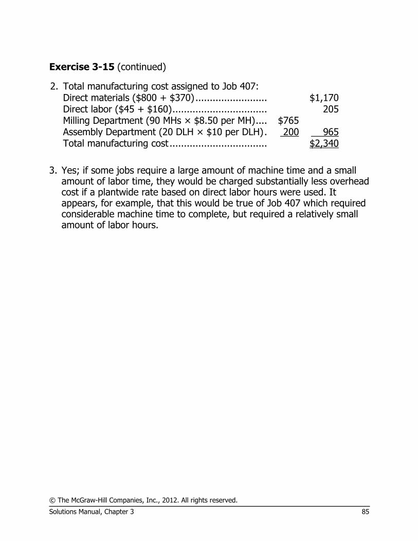
2. Total manufacturing cost assigned to Job 407: Direct materials ($800 + $370) ......................... $1,170 Direct labor ($45 + $160) ................................. 205 Milling Department (90 MHs × $8.50 per MH) .... $765 Assembly Department (20 DLH × $10 per DLH) . 200 965 Total manufacturing cost .................................. $2,340
3. Yes; if some jobs require a large amount of machine time and a small
amount of labor time, they would be charged substantially less overhead cost if a plantwide rate based on direct labor hours were used. It appears, for example, that this would be true of Job 407 which required considerable machine time to complete, but required a relatively small amount of labor hours.

© The McGraw-Hill Companies, Inc., 2012. All rights reserved.
86 Managerial Accounting, 14th edition
Exercise 3-16 (15 minutes)
1. Item (a): Actual manufacturing overhead costs for the year. Item (b): Overhead cost applied to work in process for the year. Item (c): Cost of goods manufactured for the year. Item (d): Cost of goods sold for the year.
2. Manufacturing Overhead ............................. 30,000 Cost of Goods Sold ................................ 30,000 3. The overapplied overhead will be allocated to the other accounts on the
basis of the amount of overhead applied during the year in the ending balance of each account:
Work in process ................................ $ 32,800 8 % Finished goods .................................. 41,000 10 Cost of goods sold ............................ 336,200 82 Total cost ......................................... $410,000 100 %
Using these percentages, the journal entry would be as follows:
Manufacturing Overhead ........................... 30,000 Work in Process (8% × $30,000) .......... 2,400 Finished Goods (10% × $30,000) ......... 3,000 Cost of Goods Sold (82% × $30,000) .... 24,600

© The McGraw-Hill Companies, Inc., 2012. All rights reserved.
Solutions Manual, Chapter 3 87
Exercise 3-17 (30 minutes)
1. The predetermined overhead rate is computed as follows:
Y = $106,250 + $0.75 per MH × 85,000 MHs
Estimated fixed manufacturing overhead .................. $106,250
Estimated variable manufacturing overhead
$0.75 per MH × 85,000 MHs ................................. 63,750 Estimated total manufacturing overhead cost ............ $170,000
The predetermined overhead rate is computed as follows:
Estimated total manufacturing overhead ........ $170,000 ÷ Estimated total machine-hours .................. 85,000 MHs = Predetermined overhead rate .................... $2.00 per MH
2. The amount of overhead cost applied to Work in Process for the year
would be: 80,000 machine-hours × $2.00 per machine-hour = $160,000. This amount is shown in entry (a) below:
Manufacturing Overhead (Utilities) 14,000 (a) 160,000 (Insurance) 9,000 (Maintenance) 33,000 (Indirect materials) 7,000 (Indirect labor) 65,000 (Depreciation) 40,000 Balance 8,000 Work in Process (Direct materials) 530,000 (Direct labor) 85,000 (Overhead) (a) 160,000
3. Overhead is underapplied by $8,000 for the year, as shown in the
Manufacturing Overhead account above. The entry to close out this balance to Cost of Goods Sold would be:
Cost of Goods Sold ...................................... 8,000 Manufacturing Overhead ........................... 8,000
© The McGraw-Hill Companies, Inc., 2012. All rights reserved.
88 Managerial Accounting, 14th edition
Exercise 3-17 (continued)
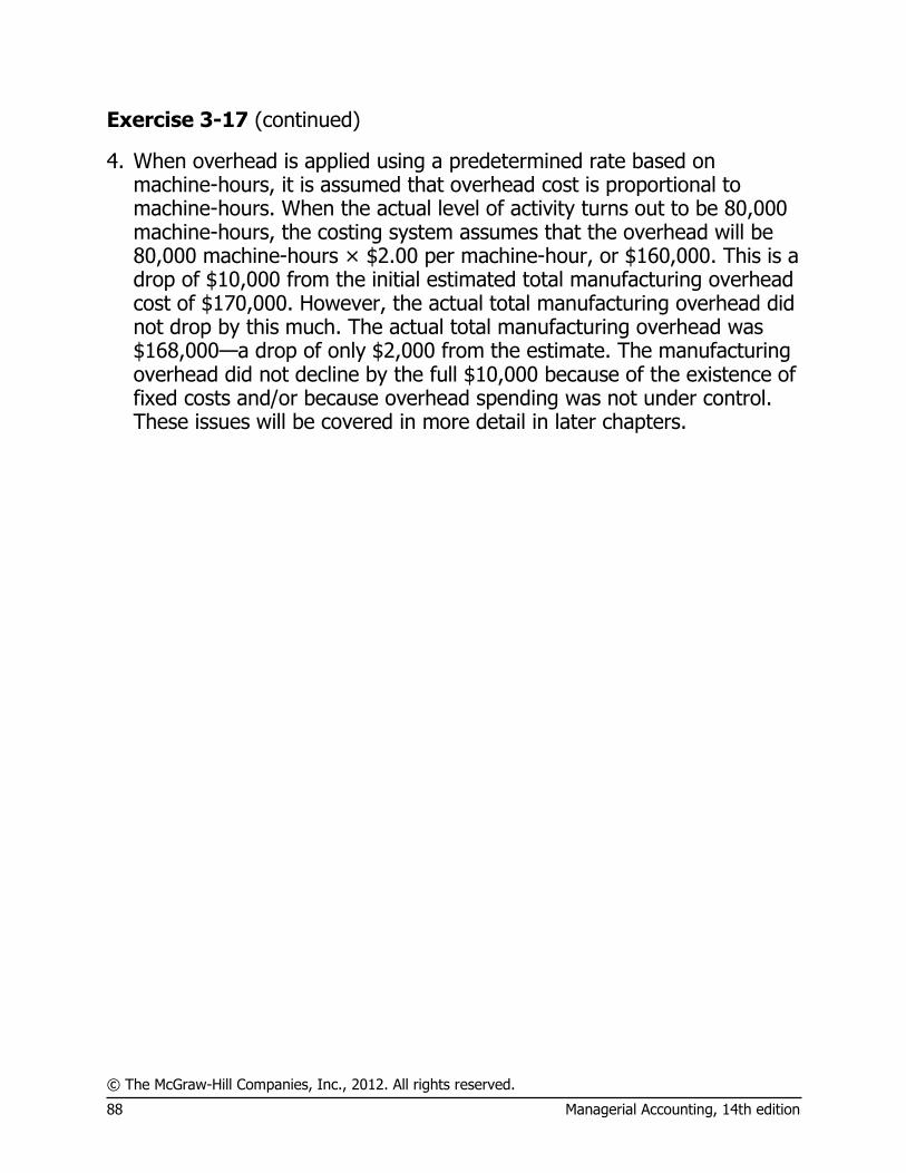
4. When overhead is applied using a predetermined rate based on machine-hours, it is assumed that overhead cost is proportional to machine-hours. When the actual level of activity turns out to be 80,000 machine-hours, the costing system assumes that the overhead will be 80,000 machine-hours × $2.00 per machine-hour, or $160,000. This is a drop of $10,000 from the initial estimated total manufacturing overhead cost of $170,000. However, the actual total manufacturing overhead did not drop by this much. The actual total manufacturing overhead was $168,000—a drop of only $2,000 from the estimate. The manufacturing overhead did not decline by the full $10,000 because of the existence of fixed costs and/or because overhead spending was not under control. These issues will be covered in more detail in later chapters.

© The McGraw-Hill Companies, Inc., 2012. All rights reserved.
Solutions Manual, Chapter 3 89
Exercise 3-18 (45 minutes)
1 a. The estimated total manufacturing overhead cost is computed as follows:
Y = $1,100,000 + $5.00 per MH × 50,000 MHs
Estimated fixed manufacturing overhead .................. $1,100,000
Estimated variable manufacturing overhead
$5.00 per MH × 50,000 MHs ................................. 250,000 Estimated total manufacturing overhead cost ............ $1,350,000
The predetermined overhead rate is computed as follows:
Estimated total manufacturing overhead ........ $1,350,000 ÷ Estimated total machine-hours (MHs) ........ 50,000 MHs = Predetermined overhead rate .................... $27.00 per MH
1 b and 1 c. Total manufacturing cost assigned to Jobs D-75 and C-100:
D-75 C-100 Direct materials ................................. $ 700,000 $ 550,000 Direct labor ....................................... 360,000 400,000
Manufacturing overhead applied ($27.00 per MH × 20,000 MHs; $27.00 per MH × 30,000 MHs) ....... 540,000 810,000
Total manufacturing cost .................... $1,600,000 $1,760,000
Bid prices for Jobs D-75 and C-100:
D-75 C-100 Total manufacturing cost .................... $1,600,000 $1,760,000 × Markup percentage ........................ 150% 150% = Bid price ........................................ $2,400,000 $2,640,000 1 d. Because the company has no beginning or ending inventories and
only Jobs D-75 and C-100 were started, completed, and sold during the year, the cost of goods sold is equal to the sum of the manufacturing costs assigned to both jobs of $3,360,000 (= $1,600,000 + $1,760,000).

© The McGraw-Hill Companies, Inc., 2012. All rights reserved.
90 Managerial Accounting, 14th edition
Exercise 3-18 (continued)
2 a. Molding Department:
The estimated total manufacturing overhead cost in the Molding Department is computed as follows:
Y = $800,000 + $5.00 per MH × 20,000 MH
Estimated fixed manufacturing overhead .................. $800,000
Estimated variable manufacturing overhead
$5.00 per MH × 20,000 MHs ................................. 100,000 Estimated total manufacturing overhead cost ............ $900,000
The predetermined overhead rate is computed as follows:
Estimated total manufacturing overhead ....... $900,000 ÷ Estimated total machine-hours .................. 20,000 MHs = Predetermined overhead rate .................... $45.00 per MH Fabrication Department:
The estimated total manufacturing overhead cost in the Fabrication Department is computed as follows:
Y = $300,000 + $5.00 per MH × 30,000 MH
Estimated fixed manufacturing overhead .................. $300,000
Estimated variable manufacturing overhead
$5.00 per MH × 30,000 MHs ................................. 150,000 Estimated total manufacturing overhead cost ............ $450,000
The predetermined overhead rate is computed as follows:
Estimated total manufacturing overhead ....... $450,000 ÷ Estimated total direct labor-hours ............. 30,000 MHs = Predetermined overhead rate .................... $15.00 per MH
© The McGraw-Hill Companies, Inc., 2012. All rights reserved.
Solutions Manual, Chapter 3 91
Exercise 3-18 (continued)
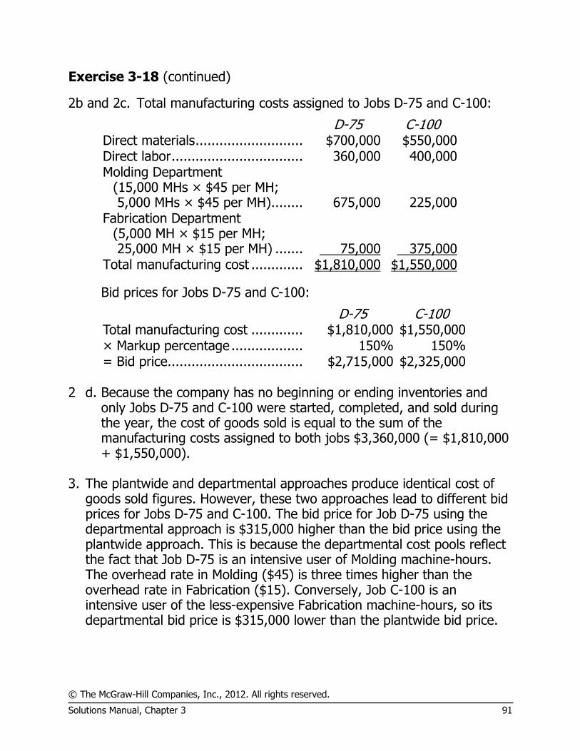
2b and 2c. Total manufacturing costs assigned to Jobs D-75 and C-100:
D-75 C-100 Direct materials ........................... $700,000 $550,000 Direct labor ................................. 360,000 400,000 Molding Department
(15,000 MHs × $45 per MH; 5,000 MHs × $45 per MH)........ 675,000 225,000
Fabrication Department (5,000 MH × $15 per MH; 25,000 MH × $15 per MH) ....... 75,000 375,000
Total manufacturing cost ............. $1,810,000 $1,550,000
Bid prices for Jobs D-75 and C-100:
D-75 C-100 Total manufacturing cost ............. $1,810,000 $1,550,000 × Markup percentage .................. 150% 150% = Bid price.................................. $2,715,000 $2,325,000 2 d. Because the company has no beginning or ending inventories and
only Jobs D-75 and C-100 were started, completed, and sold during the year, the cost of goods sold is equal to the sum of the manufacturing costs assigned to both jobs $3,360,000 (= $1,810,000 + $1,550,000).
3. The plantwide and departmental approaches produce identical cost of
goods sold figures. However, these two approaches lead to different bid prices for Jobs D-75 and C-100. The bid price for Job D-75 using the departmental approach is $315,000 higher than the bid price using the plantwide approach. This is because the departmental cost pools reflect the fact that Job D-75 is an intensive user of Molding machine-hours. The overhead rate in Molding ($45) is three times higher than the overhead rate in Fabrication ($15). Conversely, Job C-100 is an intensive user of the less-expensive Fabrication machine-hours, so its departmental bid price is $315,000 lower than the plantwide bid price.

© The McGraw-Hill Companies, Inc., 2012. All rights reserved.
92 Managerial Accounting, 14th edition
Exercise 3-18 (continued)
Whether a job-order costing system has only one plantwide overhead cost pool or numerous departmental overhead cost pools does not usually have an important impact on the accuracy of the cost of goods sold reported for the company as a whole. However, it can have a huge impact on internal decisions with respect to individual jobs, such as establishing bid prices for those jobs. Job-order costing systems that rely on one plantwide overhead cost pool are commonly used to value ending inventories and cost of goods sold for external reporting purposes, but they can create costing inaccuracies for individual jobs that adversely influence internal decision making.

© The McGraw-Hill Companies, Inc., 2012. All rights reserved.
Solutions Manual, Chapter 3 93
Exercise 3-19 (30 minutes)
1. a. Raw Materials .............................. 315,000 Accounts Payable .................... 315,000
b. Work in Process ........................... 216,000 Manufacturing Overhead .............. 54,000 Raw Materials ......................... 270,000
c. Work in Process ........................... 80,000 Manufacturing Overhead .............. 110,000 Wages and Salaries Payable .... 190,000
d. Manufacturing Overhead .............. 63,000 Accumulated Depreciation ....... 63,000
e. Manufacturing Overhead .............. 85,000 Accounts Payable .................... 85,000
f. Work in Process ........................... 300,000 Manufacturing Overhead ......... 300,000
Estimated total manufacturing overhead costPredetermined=overhead rate Estimated total amount of the allocation base
$4,320,000= =$7.50 per machine-hour
576,000 machine-hours
40,000 MHs × $7.50 per MH = $300,000. 2. Manufacturing Overhead Work in Process
(b) 54,000 (f) 300,000 (b) 216,000
(c) 110,000 (c) 80,000
(d) 63,000 (f) 300,000
(e) 85,000 3. The cost of the completed job would be $596,000 as shown in the Work
in Process T-account above. The entry for item (g) would be:
Finished Goods ................................ 596,000 Work in Process ......................... 596,000
4. The unit product cost on the job cost sheet would be: $596,000 ÷ 8,000 units = $74.50 per unit.

© The McGraw-Hill Companies, Inc., 2012. All rights reserved.
94 Managerial Accounting, 14th edition
Exercise 3-20 (30 minutes)
1. Since $320,000 of studio overhead cost was applied to Work in Process on the basis of $200,000 of direct staff costs, the apparent predetermined overhead rate was 160%:
Studio overhead applied $320,000=
Total amount of the allocation base $200,000 direct staff costs
=160% of direct staff costs
2. The Krimmer Corporation Headquarters project is the only job remaining
in Work in Process at the end of the month; therefore, the entire $40,000 balance in the Work in Process account at that point must apply to it. Recognizing that the predetermined overhead rate is 160% of direct staff costs, the following computation can be made:
Total cost added to the Krimmer Corporation Headquarters project ..... $40,000
Less: Direct staff costs ................................ $13,500 Studio overhead cost ($13,500 × 160%) ........................... 21,600 35,100 Costs of subcontracted work ............... $ 4,900
With this information, we can now complete the job cost sheet for the Krimmer Corporation Headquarters project:
Costs of subcontracted work ........... $ 4,900 Direct staff costs ............................ 13,500 Studio overhead ............................. 21,600 Total cost to January 31 ................. $40,000
© The McGraw-Hill Companies, Inc., 2012. All rights reserved.
Solutions Manual, Chapter 3 95
Problem 3-21 (30 minutes)
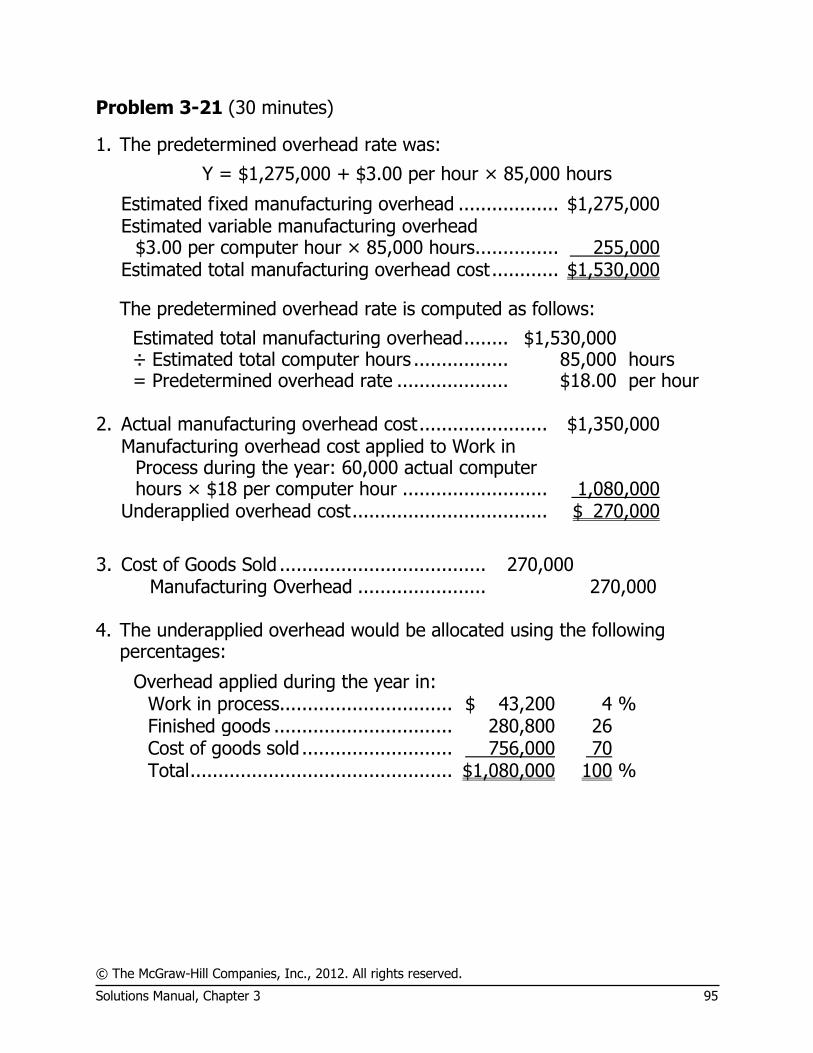
1. The predetermined overhead rate was:
Y = $1,275,000 + $3.00 per hour × 85,000 hours
Estimated fixed manufacturing overhead .................. $1,275,000
Estimated variable manufacturing overhead
$3.00 per computer hour × 85,000 hours............... 255,000 Estimated total manufacturing overhead cost ............ $1,530,000
The predetermined overhead rate is computed as follows:
Estimated total manufacturing overhead ........ $1,530,000 ÷ Estimated total computer hours ................. 85,000 hours = Predetermined overhead rate .................... $18.00 per hour
2. Actual manufacturing overhead cost ....................... $1,350,000
Manufacturing overhead cost applied to Work in Process during the year: 60,000 actual computer hours × $18 per computer hour .......................... 1,080,000
Underapplied overhead cost ................................... $ 270,000
3. Cost of Goods Sold ..................................... 270,000 Manufacturing Overhead ....................... 270,000 4. The underapplied overhead would be allocated using the following
percentages:
Overhead applied during the year in: Work in process............................... $ 43,200 4 % Finished goods ................................ 280,800 26 Cost of goods sold ........................... 756,000 70 Total ............................................... $1,080,000 100 %

© The McGraw-Hill Companies, Inc., 2012. All rights reserved.
96 Managerial Accounting, 14th edition
Problem 3-21 (continued) The entry to record the allocation of the underapplied overhead is:
Work In Process (4% × $270,000) ......... 10,800 Finished Goods (26% × $270,000) ......... 70,200 Cost of Goods Sold (70% × $270,000) ... 189,000
Manufacturing Overhead ................... 270,000 5. Comparing the two methods of closing underapplied overhead:
Cost of goods sold if the underapplied overhead is closed directly to cost of goods sold ($2,800,000 + $270,000) ................................. $3,070,000
Cost of goods sold if the underapplied overhead is allocated among the accounts ($2,800,000 + $189,000) ....................................................... 2,989,000
Difference in cost of goods sold .......................... $ 81,000
Thus, net operating income will be $81,000 greater if the underapplied overhead is allocated among Work In Process, Finished Goods, and Cost of Goods Sold rather than closed directly to Cost of Goods Sold.

© The McGraw-Hill Companies, Inc., 2012. All rights reserved.
Solutions Manual, Chapter 3 97
Problem 3-22 (30 minutes) 1. Cost of Goods Manufactured Direct materials: Raw materials inventory, beginning* ........... $ 50,000 Add: Purchases of raw materials* ............... 260,000 Total raw materials available ...................... 310,000 Deduct: Raw materials inventory, ending* ... 40,000 Raw materials used in production ............... 270,000 Direct labor .................................................... 65,000 Manufacturing overhead applied to work in
process inventory* ....................................... 340,000 Total manufacturing costs* ............................. 675,000 Add: Beginning work in process inventory........ 48,000 723,000 Deduct: Ending work in process inventory*...... 33,000 Cost of goods manufactured ........................... $690,000 2. Cost of Goods Sold Finished goods inventory, beginning* .............. $ 30,000 Add: Cost of goods manufactured ................... 690,000 Cost of goods available for sale* ..................... 720,000 Deduct: Finished goods inventory, ending........ 55,000 Unadjusted cost of goods sold* ....................... 665,000 Add: Underapplied overhead ........................... 10,000 Adjusted cost of goods sold ............................ $675,000
3.
Valenko Company Income Statement
Sales ......................................................... $1,085,000 Cost of goods sold ($665,000 + $10,000) .... 675,000 Gross margin .............................................. 410,000 Selling and administrative expenses:
Selling expenses* .................................... $215,000 Administrative expense* ........................... 160,000 375,000
Net operating income* ................................ $ 35,000
* Given
© The McGraw-Hill Companies, Inc., 2012. All rights reserved.
98 Managerial Accounting, 14th edition
Problem 3-23 (45 minutes)
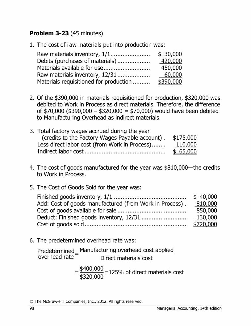
1. The cost of raw materials put into production was:
Raw materials inventory, 1/1 ....................... $ 30,000 Debits (purchases of materials) ................... 420,000 Materials available for use ........................... 450,000 Raw materials inventory, 12/31 ................... 60,000 Materials requisitioned for production .......... $390,000
2. Of the $390,000 in materials requisitioned for production, $320,000 was
debited to Work in Process as direct materials. Therefore, the difference of $70,000 ($390,000 – $320,000 = $70,000) would have been debited to Manufacturing Overhead as indirect materials.
3. Total factory wages accrued during the year
(credits to the Factory Wages Payable account) .. $175,000 Less direct labor cost (from Work in Process) ........ 110,000 Indirect labor cost ............................................... $ 65,000
4. The cost of goods manufactured for the year was $810,000—the credits
to Work in Process. 5. The Cost of Goods Sold for the year was:
Finished goods inventory, 1/1 .......................................... $ 40,000 Add: Cost of goods manufactured (from Work in Process) . 810,000 Cost of goods available for sale ........................................ 850,000 Deduct: Finished goods inventory, 12/31 .......................... 130,000 Cost of goods sold ........................................................... $720,000
6. The predetermined overhead rate was:
Manufacturing overhead cost appliedPredetermined=overhead rate Direct materials cost
$400,000= =125% of direct materials cost
$320,000

© The McGraw-Hill Companies, Inc., 2012. All rights reserved.
Solutions Manual, Chapter 3 99
Problem 3-23 (continued)
7. Manufacturing overhead was overapplied by $15,000, computed as follows:
Actual manufacturing overhead cost for the year (debits) ....................................................................... $385,000
Applied manufacturing overhead cost (from Work in Process—this would be the credits to the Manufacturing Overhead account) ................................ 400,000
Overapplied overhead ..................................................... $(15,000)
8. The ending balance in Work in Process is $90,000. Direct labor makes
up $18,000 of this balance, and manufacturing overhead makes up $40,000. The computations are:
Balance, Work in Process, 12/31 ................................. $90,000 Less: Direct materials cost (given) ............................... (32,000)
Manufacturing overhead cost ($32,000 × 125%) .......................................... (40,000)
Direct labor cost (remainder) ...................................... $18,000

© The McGraw-Hill Companies, Inc., 2012. All rights reserved.
100 Managerial Accounting, 14th edition
Problem 3-24 (60 minutes)
1. a.
Estimated total manufacturing overhead costPredetermined=overhead rate Estimated total amount of the allocation base
$126,000= =150% of direct labor cost
$84,000 direct labor cost
b. Actual manufacturing overhead costs: Insurance, factory .................................... $ 7,000 Depreciation of equipment........................ 18,000 Indirect labor ........................................... 42,000 Property taxes ......................................... 9,000 Maintenance ............................................ 11,000 Rent, building .......................................... 36,000 Total actual costs ....................................... 123,000
Applied manufacturing overhead costs:
$80,000 × 150% ..................................... 120,000 Underapplied overhead ............................... $ 3,000
2.
Pacific Manufacturing Company Schedule of Cost of Goods Manufactured
Direct materials: Raw materials inventory, beginning ................. $ 21,000 Add: Purchases of raw materials ..................... 133,000 Total raw materials available .......................... 154,000 Deduct: Raw materials inventory, ending ........ 16,000 Raw materials used in production ................... $138,000
Direct labor ...................................................... 80,000 Manufacturing overhead applied to work in
process ......................................................... 120,000 Total manufacturing cost .................................. 338,000 Add: Work in process, beginning ....................... 44,000 382,000 Deduct: Work in process, ending ....................... 40,000 Cost of goods manufactured ............................. $342,000
© The McGraw-Hill Companies, Inc., 2012. All rights reserved.
Solutions Manual, Chapter 3 101
Problem 3-24 (continued)
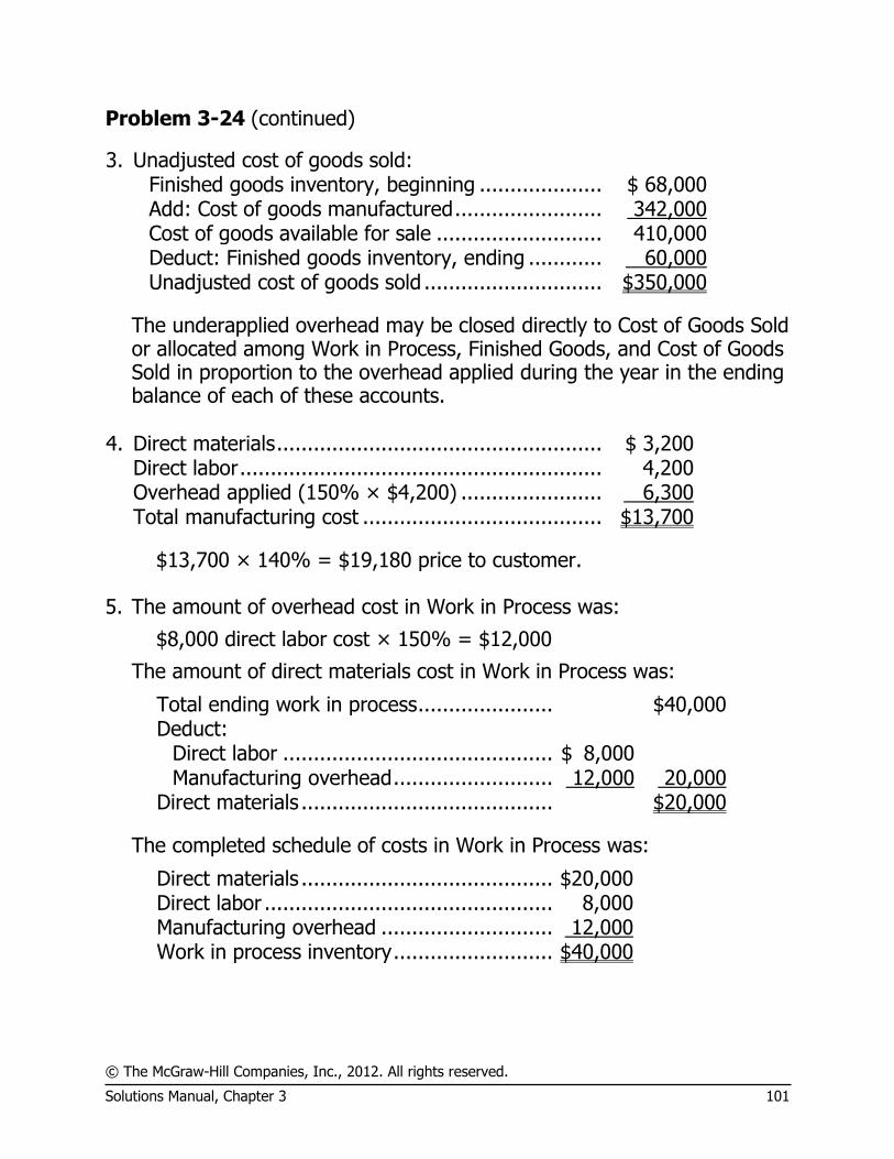
3. Unadjusted cost of goods sold: Finished goods inventory, beginning .................... $ 68,000 Add: Cost of goods manufactured ........................ 342,000 Cost of goods available for sale ........................... 410,000 Deduct: Finished goods inventory, ending ............ 60,000 Unadjusted cost of goods sold ............................. $350,000
The underapplied overhead may be closed directly to Cost of Goods Sold or allocated among Work in Process, Finished Goods, and Cost of Goods Sold in proportion to the overhead applied during the year in the ending balance of each of these accounts.
4. Direct materials ..................................................... $ 3,200 Direct labor ........................................................... 4,200 Overhead applied (150% × $4,200) ....................... 6,300 Total manufacturing cost ....................................... $13,700
$13,700 × 140% = $19,180 price to customer. 5. The amount of overhead cost in Work in Process was:
$8,000 direct labor cost × 150% = $12,000
The amount of direct materials cost in Work in Process was:
Total ending work in process ...................... $40,000 Deduct:
Direct labor ............................................ $ 8,000 Manufacturing overhead .......................... 12,000 20,000
Direct materials ......................................... $20,000
The completed schedule of costs in Work in Process was:
Direct materials ......................................... $20,000 Direct labor ............................................... 8,000 Manufacturing overhead ............................ 12,000 Work in process inventory .......................... $40,000

© The McGraw-Hill Companies, Inc., 2012. All rights reserved.
102 Managerial Accounting, 14th edition
Problem 3-25 (120 minutes)
1. a. Raw Materials ...................................... 142,000 Accounts Payable ........................... 142,000
b. Work in Process ................................... 150,000 Raw Materials ................................. 150,000
c. Manufacturing Overhead ...................... 21,000 Accounts Payable ........................... 21,000
d. Work in Process ................................... 216,000 Manufacturing Overhead ...................... 90,000 Salaries Expense .................................. 145,000 Salaries and Wages Payable ............ 451,000
e. Manufacturing Overhead ...................... 15,000 Accounts Payable ........................... 15,000
f. Advertising Expense ............................. 130,000 Accounts Payable ........................... 130,000
g. Manufacturing Overhead ...................... 45,000 Depreciation Expense........................... 5,000 Accumulated Depreciation ............... 50,000
h. Manufacturing Overhead ...................... 72,000 Rent Expense ...................................... 18,000 Accounts Payable ........................... 90,000
i. Miscellaneous Expense ......................... 17,000 Accounts Payable ........................... 17,000 j. Work in Process ................................... 240,000 Manufacturing Overhead ................. 240,000
Estimated total manufacturing overhead cost $248,000=
Estimated direct materials cost $155,000
160% of direct=materials cost.
$150,000 direct materials cost × 160% = $240,000 applied.
© The McGraw-Hill Companies, Inc., 2012. All rights reserved.
Solutions Manual, Chapter 3 103
Problem 3-25 (continued)
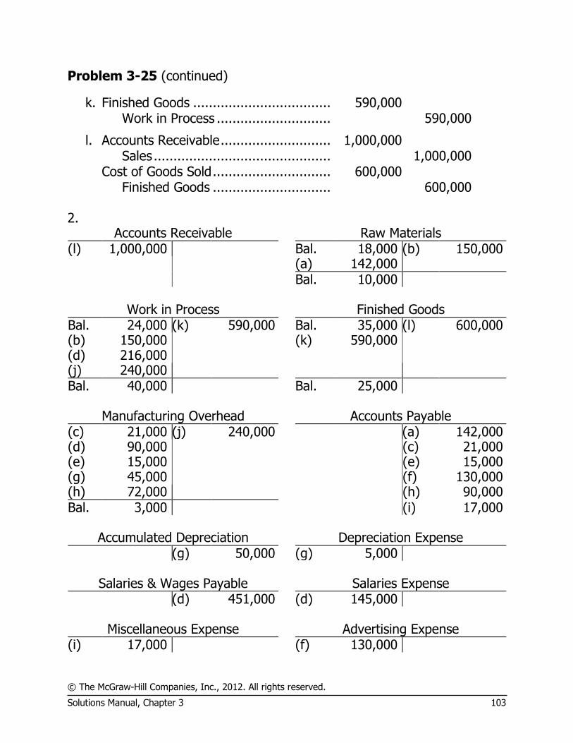
k. Finished Goods ................................... 590,000 Work in Process ............................. 590,000
l. Accounts Receivable ............................ 1,000,000 Sales ............................................. 1,000,000 Cost of Goods Sold .............................. 600,000 Finished Goods .............................. 600,000
2.
Accounts Receivable Raw Materials (l) 1,000,000 Bal. 18,000 (b) 150,000 (a) 142,000 Bal. 10,000
Work in Process Finished Goods Bal. 24,000 (k) 590,000 Bal. 35,000 (l) 600,000 (b) 150,000 (k) 590,000 (d) 216,000 (j) 240,000 Bal. 40,000 Bal. 25,000
Manufacturing Overhead Accounts Payable (c) 21,000 (j) 240,000 (a) 142,000 (d) 90,000 (c) 21,000 (e) 15,000 (e) 15,000 (g) 45,000 (f) 130,000 (h) 72,000 (h) 90,000 Bal. 3,000 (i) 17,000
Accumulated Depreciation Depreciation Expense (g) 50,000 (g) 5,000
Salaries & Wages Payable Salaries Expense (d) 451,000 (d) 145,000
Miscellaneous Expense Advertising Expense (i) 17,000 (f) 130,000

© The McGraw-Hill Companies, Inc., 2012. All rights reserved.
104 Managerial Accounting, 14th edition
Problem 3-25 (continued)
Rent Expense Cost of Goods Sold (h) 18,000 (l) 600,000
Sales (l) 1,000,000 3.
Southworth Company Schedule of Cost of Goods Manufactured
Direct materials: Raw materials inventory, beginning ................... $ 18,000 Add: Purchases of raw materials ........................ 142,000 Materials available for use ................................. 160,000 Deduct: Raw materials inventory, ending ........... 10,000 Materials used in production .............................. $150,000 Direct labor ......................................................... 216,000
Manufacturing overhead applied to work in
process ............................................................ 240,000 Total manufacturing cost ..................................... 606,000 Add: Work in process, beginning .......................... 24,000 630,000 Deduct: Work in process, ending .......................... 40,000 Cost of goods manufactured ................................ $590,000
4.
Cost of Goods Sold .......................................... 3,000 Manufacturing Overhead............................. 3,000
Schedule of cost of goods sold: Finished goods inventory, beginning .............. $ 35,000 Add: Cost of goods manufactured .................. 590,000 Cost of goods available for sale ..................... 625,000 Deduct: Finished goods inventory, ending ...... 25,000 Unadjusted cost of goods sold ....................... 600,000 Add: Underapplied overhead ......................... 3,000 Adjusted cost of goods sold ........................... $603,000

© The McGraw-Hill Companies, Inc., 2012. All rights reserved.
Solutions Manual, Chapter 3 105
Problem 3-25 (continued)
5.
Southworth Company Income Statement
Sales .......................................................... $1,000,000 Cost of goods sold ....................................... 603,000 Gross margin .............................................. 397,000 Selling and administrative expenses: Salaries expense ....................................... $145,000 Advertising expense .................................. 130,000 Depreciation expense ................................ 5,000 Rent expense ........................................... 18,000 Miscellaneous expense .............................. 17,000 315,000 Net operating income .................................. $ 82,000
6. Direct materials ............................................................. $ 3,600 Direct labor (400 hours × $11 per hour) ......................... 4,400 Manufacturing overhead cost applied (160% × $3,600) ... 5,760 Total manufacturing cost ............................................... 13,760 Add markup (75% × $13,760) ....................................... 10,320 Total billed price of Job 218 ........................................... $24,080
$24,080 ÷ 500 units = $48.16 per unit.

© The McGraw-Hill Companies, Inc., 2012. All rights reserved.
106 Managerial Accounting, 14th edition
Problem 3-26 (30 minutes)
1. Preparation Department:
The estimated total manufacturing overhead cost in the Preparation Department is computed as follows:
Y = $256,000 + $2.00 per MH × 80,000 MH
Estimated fixed manufacturing overhead .................. $256,000
Estimated variable manufacturing overhead:
$2.00 per MH × 80,000 MHs ................................. 160,000 Estimated total manufacturing overhead cost ............ $416,000
The predetermined overhead rate is computed as follows:
Estimated total manufacturing overhead ...... $416,000 ÷ Estimated total machine-hours ................ 80,000 MHs = Predetermined overhead rate .................. $5.20 per MH
Fabrication Department:
The estimated total manufacturing overhead cost in the Fabrication Department is computed as follows:
Y = $520,000 + $4.00 per DLH × 50,000 DLH
Estimated fixed manufacturing overhead .................. $520,000
Estimated variable manufacturing overhead:
$4.00 per DLH × 50,000 DLHs ............................... 200,000 Estimated total manufacturing overhead cost ............ $720,000
The predetermined overhead rate is computed as follows:
Estimated total manufacturing overhead ...... $720,000 ÷ Estimated total machine-hours ................ 50,000 DLHs = Predetermined overhead rate .................. $14.40 per DLH

© The McGraw-Hill Companies, Inc., 2012. All rights reserved.
Solutions Manual, Chapter 3 107
Problem 3-26 (continued)
2. Preparation Department overhead applied: 350 machine-hours × $5.20 per machine-hour ..... $1,820 Fabrication Department overhead applied: 130 direct labor-hours × $14.40 per labor-hour .... 1,872 Total overhead cost ............................................... $3,692
3. Total cost of Job 127:
Preparation Fabrication Total Direct materials ................ $ 940 $1,200 $2,140 Direct labor ...................... 710 980 1,690 Manufacturing overhead ... 1,820 1,872 3,692 Total cost ........................ $3,470 $4,052 $7,522
Unit product cost for Job 127: Total manufacturing cost .......................... $7,522 ÷ Number of units in the job ..................... 25 units = Unit product cost .................................. $300.88 per unit
4.
Preparation Fabrication Manufacturing overhead cost incurred ..... $390,000 $740,000 Manufacturing overhead cost applied:
73,000 machine-hours × $5.20 per machine-hour ................................... 379,600
54,000 direct labor-hours × $14.40 per direct labor-hour ......................... 777,600
Underapplied (or overapplied) overhead .. $ 10,400 $(37,600)

© The McGraw-Hill Companies, Inc., 2012. All rights reserved.
108 Managerial Accounting, 14th edition
Problem 3-27 (45 minutes)
1. a. Raw Materials ........................................ 160,000 Accounts Payable .............................. 160,000
b. Work in Process ..................................... 120,000 Manufacturing Overhead ........................ 20,000 Raw Materials ................................... 140,000
c. Work in Process ..................................... 90,000 Manufacturing Overhead ........................ 60,000 Sales Commissions Expense ................... 20,000 Salaries Expense .................................... 50,000 Salaries and Wages Payable .............. 220,000
d. Manufacturing Overhead ........................ 13,000 Insurance Expense................................. 5,000 Prepaid Insurance ............................. 18,000
e. Manufacturing Overhead ........................ 10,000 Accounts Payable .............................. 10,000
f. Advertising Expense ............................... 15,000 Accounts Payable .............................. 15,000
g. Manufacturing Overhead ........................ 20,000 Depreciation Expense ............................. 5,000 Accumulated Depreciation ................. 25,000
h. Work in Process ..................................... 110,000 Manufacturing Overhead ................... 110,000
Estimated total manufacturing overhead cost £99,000= =£2.20 per MH
Estimated total amount of the allocation base 45,000 MHs
50,000 actual MHs × £2.20 per MH = £110,000 overhead applied.

© The McGraw-Hill Companies, Inc., 2012. All rights reserved.
Solutions Manual, Chapter 3 109
Problem 3-27 (continued)
i. Finished Goods .................................. 310,000 Work in Process ............................ 310,000
j. Accounts Receivable ........................... 498,000 Sales ............................................ 498,000 Cost of Goods Sold ............................. 308,000 Finished Goods ............................. 308,000
2.
Raw Materials Work in Process Bal. 10,000 (b) 140,000 Bal. 4,000 (i) 310,000 (a) 160,000 (b) 120,000 (c) 90,000 (h) 110,000 Bal. 30,000 Bal. 14,000
Finished Goods Manufacturing Overhead Bal. 8,000 (j) 308,000 (b) 20,000 (h) 110,000 (i) 310,000 (c) 60,000 (d) 13,000 (e) 10,000 (g) 20,000 Bal. 10,000 Bal. 13,000
Cost of Goods Sold (j) 308,000 3. Manufacturing overhead is underapplied by £13,000 for the year. The
entry to close this balance to Cost of Goods Sold would be:
Cost of Goods Sold ..................................... 13,000 Manufacturing Overhead ........................ 13,000

© The McGraw-Hill Companies, Inc., 2012. All rights reserved.
110 Managerial Accounting, 14th edition
Problem 3-27 (continued)
4. Sovereign Millwork, Ltd.
Income Statement For the Year Ended June 30
Sales .............................................................. £498,000 Cost of goods sold (£308,000 + £13,000) ......... 321,000 Gross margin ................................................... 177,000 Selling and administrative expenses:
Sales commissions ........................................ £20,000 Administrative salaries ................................... 50,000 Insurance expense ........................................ 5,000 Advertising expenses..................................... 15,000 Depreciation expense .................................... 5,000 95,000
Net operating income ...................................... £ 82,000

© The McGraw-Hill Companies, Inc., 2012. All rights reserved.
Solutions Manual, Chapter 3 111
Problem 3-28 (60 minutes)
1. and 2.
Cash Accounts Receivable Bal. 15,000 (c) 225,000 Bal. 40,000 (l) 445,000 (l) 445,000 (m) 150,000 (k) 450,000 Bal. 85,000 Bal. 45,000
Raw Materials Work in Process Bal. 25,000 (b) 90,000 Bal. 30,000 (j) 310,000 (a) 80,000 (b) 85,000 (c) 120,000 (i) 96,000 Bal. 15,000 Bal. 21,000
Finished Goods Prepaid Insurance Bal. 45,000 (k) 300,000 Bal. 5,000 (f) 4,800 (j) 310,000 Bal. 55,000 Bal. 200
Buildings & Equipment Accumulated Depreciation Bal. 500,000 Bal. 210,000 (e) 30,000 Bal. 240,000
Manufacturing Overhead Accounts Payable (b) 5,000 (i)* 96,000 (m) 150,000 Bal. 75,000 (c) 30,000 (a) 80,000 (d) 12,000 (d) 12,000 (e) 25,000 (g) 40,000 (f) 4,000 (h) 17,000 (h) 17,000 Bal. 3,000 Bal. 74,000
$80,000* = 80% of direct labor cost; $120,000 × 0.80 = $96,000.
$100,000
Retained Earnings Capital Stock Bal. 125,000 Bal. 250,000

© The McGraw-Hill Companies, Inc., 2012. All rights reserved.
112 Managerial Accounting, 14th edition
Problem 3-28 (continued)
Salaries Expense Depreciation Expense (c) 75,000 (e) 5,000
Insurance Expense Shipping Expense (f) 800 (g) 40,000
Cost of Goods Sold Sales (k) 300,000 (k) 450,000 3. Manufacturing overhead was overapplied by $3,000 for the year. This
balance would be allocated between Work in Process, Finished Goods, and Cost of Goods Sold in proportion to the ending balances in these accounts. The allocation would be:
Work in Process, 12/31 ................ $ 21,000 5.6 % Finished Goods, 12/31 .................. 55,000 14.6 Cost of Goods Sold, 12/31 ............ 300,000 79.8 $376,000 100.0 %
Manufacturing Overhead .............................. 3,000 Work in Process (5.6% × $3,000) ............ 168 Finished Goods (14.6% × $3,000) ........... 438 Cost of Goods Sold (79.8% × $3,000) ...... 2,394
4.
Fantastic Props, Inc. Income Statement
For the Year Ended December 31
Sales ............................................................ $450,000 Cost of goods sold ($300,000 – $2,394) .......... 297,606 Gross margin ................................................. 152,394 Selling and administrative expenses:
Salaries expense ......................................... $75,000 Depreciation expense .................................. 5,000 Insurance expense ...................................... 800 Shipping expense ........................................ 40,000 120,800
Net operating income .................................... $ 31,594
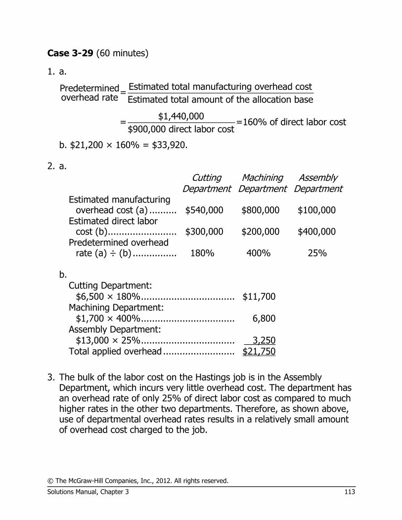
© The McGraw-Hill Companies, Inc., 2012. All rights reserved.
Solutions Manual, Chapter 3 113
Case 3-29 (60 minutes)
1. a.
Estimated total manufacturing overhead costPredetermined=overhead rate Estimated total amount of the allocation base
$1,440,000= =160% of direct labor cost
$900,000 direct labor cost
b. $21,200 × 160% = $33,920. 2. a.
Cutting
Department Machining
Department Assembly
Department
Estimated manufacturing
overhead cost (a) .......... $540,000 $800,000 $100,000
Estimated direct labor
cost (b) ......................... $300,000 $200,000 $400,000
Predetermined overhead
rate (a) ÷ (b) ................ 180% 400% 25% b.
Cutting Department: $6,500 × 180% .................................. $11,700 Machining Department: $1,700 × 400% .................................. 6,800 Assembly Department: $13,000 × 25% .................................. 3,250 Total applied overhead .......................... $21,750
3. The bulk of the labor cost on the Hastings job is in the Assembly
Department, which incurs very little overhead cost. The department has an overhead rate of only 25% of direct labor cost as compared to much higher rates in the other two departments. Therefore, as shown above, use of departmental overhead rates results in a relatively small amount of overhead cost charged to the job.

© The McGraw-Hill Companies, Inc., 2012. All rights reserved.
114 Managerial Accounting, 14th edition
Case 3-29 (continued)
However, use of a plantwide overhead rate in effect redistributes overhead costs proportionately between the three departments (at 160% of direct labor cost) and results in a large amount of overhead cost being charged to the Hastings job, as shown in Part 1. This may explain why the company bid too high and lost the job. Too much overhead cost was assigned to the job for the kind of work being done on the job in the plant.
If a plantwide overhead rate is being used, the company will tend to charge too little overhead cost to jobs that require a large amount of labor in the Cutting or Machining Departments. The reason is that the plantwide overhead rate (160%) is much lower than the rates if these departments were considered separately.
4. The company’s bid price was:
Direct materials .............................................. $ 18,500 Direct labor .................................................... 21,200 Manufacturing overhead applied (above) ......... 33,920 Total manufacturing cost ................................ 73,620 Bidding rate ................................................... × 1.5 Total bid price ................................................ $110,430
If departmental overhead rates had been used, the bid price would have
been:
Direct materials .............................................. $ 18,500 Direct labor .................................................... 21,200 Manufacturing overhead applied (above) ......... 21,750 Total manufacturing cost ................................ 61,450 Bidding rate ................................................... × 1.5 Total bid price ................................................ $ 92,175
Note that if departmental overhead rates had been used, Lenko Products would have been the low bidder on the Hastings job since the competitor underbid Lenko by only $10,000.

© The McGraw-Hill Companies, Inc., 2012. All rights reserved.
Solutions Manual, Chapter 3 115
Case 3-29 (continued)
5. a. Actual overhead cost ....................................... $1,482,000 Applied overhead cost ($870,000 × 160%) ....... 1,392,000 Underapplied overhead cost ............................. $ 90,000
b.
Department Cutting Machining Assembly Total Plant
Actual overhead cost ............ $560,000 $830,000 $92,000 $1,482,000 Applied overhead cost:
$320,000 × 180% ............. 576,000 $210,000 × 400% ............. 840,000 $340,000 × 25% ............... 85,000 1,501,000
Underapplied (overapplied) overhead cost ................... $(16,000) $(10,000) $ 7,000 $ (19,000)

© The McGraw-Hill Companies, Inc., 2012. All rights reserved.
116 Managerial Accounting, 14th edition
Case 3-30 (45 minutes)
1. Shaving 5% off the estimated direct labor-hours in the predetermined overhead rate will result in an artificially high overhead rate, which is likely to result in overapplied overhead for the year. The cumulative effect of overapplying the overhead throughout the year is all recognized in December when the balance in the Manufacturing Overhead account is closed out to Cost of Goods Sold. If the balance were closed out every month or every quarter, this effect would be dissipated over the course of the year.
2. This question may generate lively debate. Where should Cristin
Madsen’s loyalties lie? Is she working for the general manager of the division or for the corporate controller? Is there anything wrong with the “Christmas bonus”? How far should Cristin go in bucking her boss on a new job?
While individuals can certainly disagree about what Cristin should do, some of the facts are indisputable. First, the practice of understating direct labor-hours results in artificially inflating the overhead rate. This has the effect of inflating the cost of goods sold figures in all months prior to December and overstating the costs of inventories. In December, the adjustment for overapplied overhead provides a big boost to net operating income. Therefore, the practice results in distortions in the pattern of net operating income over the year. In addition, since all of the adjustment is taken to Cost of Goods Sold, inventories are still overstated at year-end. This means that retained earnings is also overstated.
While Cristin is in an extremely difficult position, her responsibilities under the IMA’s Statement of Ethical Professional Practice seem to be clear. The Credibility standard states that management accountants have a responsibility to “disclose all relevant information that could reasonably be expected to influence an intended user’s understanding of the reports, analyses, or recommendations.” Cristin should discuss this situation with her immediate supervisor in the controller’s office at corporate headquarters. This step may bring her into direct conflict with the general manager of the division, so it would be a very difficult decision for her to make.

© The McGraw-Hill Companies, Inc., 2012. All rights reserved.
Solutions Manual, Chapter 3 117
Case 3-30 (continued)
In the actual situation that this case is based on, the corporate controller’s staff were aware of the general manager’s accounting tricks, but top management of the company supported the general manager because “he comes through with the results” and could be relied on to hit the annual profit targets for his division. Personally, we would be very uncomfortable supporting a manager who will resort to deliberate distortions to achieve “results.” If the manager will pull tricks in this area, what else might he be doing that is questionable or even perhaps illegal?
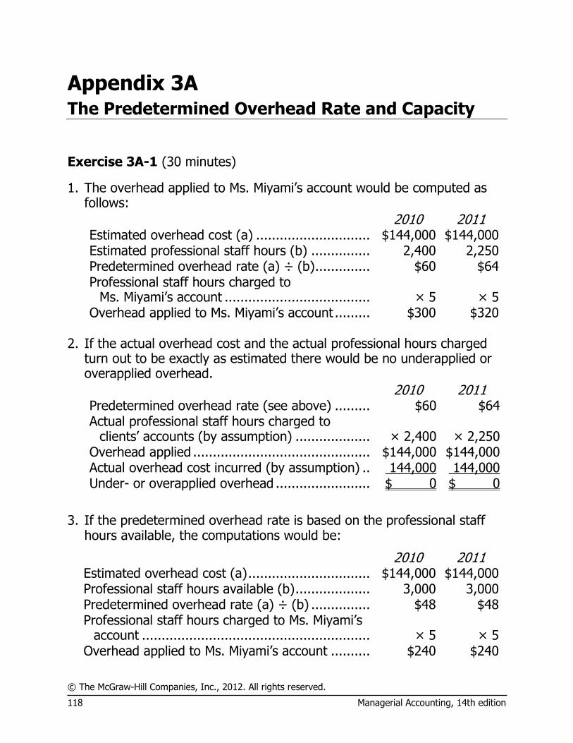
© The McGraw-Hill Companies, Inc., 2012. All rights reserved.
118 Managerial Accounting, 14th edition
Appendix 3A The Predetermined Overhead Rate and Capacity
Exercise 3A-1 (30 minutes)
1. The overhead applied to Ms. Miyami’s account would be computed as follows:
2010 2011 Estimated overhead cost (a) ............................. $144,000 $144,000 Estimated professional staff hours (b) ............... 2,400 2,250 Predetermined overhead rate (a) ÷ (b) .............. $60 $64 Professional staff hours charged to
Ms. Miyami’s account ..................................... × 5 × 5 Overhead applied to Ms. Miyami’s account ......... $300 $320
2. If the actual overhead cost and the actual professional hours charged
turn out to be exactly as estimated there would be no underapplied or overapplied overhead.
2010 2011 Predetermined overhead rate (see above) ......... $60 $64 Actual professional staff hours charged to
clients’ accounts (by assumption) ................... × 2,400 × 2,250 Overhead applied ............................................. $144,000 $144,000 Actual overhead cost incurred (by assumption) .. 144,000 144,000 Under- or overapplied overhead ........................ $ 0 $ 0
3. If the predetermined overhead rate is based on the professional staff
hours available, the computations would be:
2010 2011 Estimated overhead cost (a) ............................... $144,000 $144,000 Professional staff hours available (b) ................... 3,000 3,000 Predetermined overhead rate (a) ÷ (b) ............... $48 $48 Professional staff hours charged to Ms. Miyami’s
account .......................................................... × 5 × 5 Overhead applied to Ms. Miyami’s account .......... $240 $240

© The McGraw-Hill Companies, Inc., 2012. All rights reserved.
Solutions Manual, Appendix 3A 119
Problem 3A-1 (continued)
4. If the actual overhead cost and the actual professional staff hours charged to clients’ accounts turn out to be exactly as estimated overhead would be underapplied as shown below.
2010 2011 Predetermined overhead rate (see 3 above) (a) ... $48 $48 Actual professional staff hours charged to
clients’ accounts (by assumption) (b) ............... × 2,250 × 2,400 Overhead applied (a) × (b) ................................ $108,000 $115,200 Actual overhead cost incurred (by assumption) .... 144,000 144,000 Underapplied overhead ...................................... $ 36,000 $ 28,800
The underapplied overhead is best interpreted in this situation as the cost of idle capacity. Proponents of this method of computing predetermined overhead rates suggest that the underapplied overhead be treated as a period expense that would be separately disclosed on the income statement as Cost of Unused Capacity.

© The McGraw-Hill Companies, Inc., 2012. All rights reserved.
120 Managerial Accounting, 14th edition
Exercise 3A-2 (30 minutes)
1. There were no beginning or ending inventories, so all of the jobs were started, finished, and sold during the month. Therefore cost of goods sold equals the total manufacturing cost. We can verify that by computing the cost of goods sold as shown below:
Manufacturing costs charged to jobs: Direct materials ........................................... $ 5,350 Direct labor (all variable) .............................. 8,860 Manufacturing overhead applied
(150 hours × $82 hour) ............................. 12,300 Total manufacturing cost charged to jobs ........ 26,510 Add: Beginning work in process inventory ........ 0 26,510 Deduct: Ending work in process inventory ....... 0 Cost of goods manufactured ........................... $26,510
Beginning finished goods inventory ................. $ 0 Add: Cost of goods manufactured ................... 26,510 Goods available for sale .................................. 26,510 Deduct: Ending finished goods inventory ......... 0 Cost of goods sold .......................................... $26,510
At the end of the month, overhead was underapplied by $1,920 as shown below:
Manufacturing overhead incurred .................... $14,220 Manufacturing overhead applied
(150 hours × $82 hour) ............................... 12,300 Overhead underapplied................................... $ 1,920

© The McGraw-Hill Companies, Inc., 2012. All rights reserved.
Solutions Manual, Appendix 3A 121
Exercise 3A-2 (continued)
Consequently, the income statement would appear as follows:
Wixis Cabinets Income Statement
Sales .................................................... $43,740 Cost of goods sold (see above) .............. 26,510 Gross margin ........................................ 17,230 Underapplied manufacturing overhead ... $1,920 Selling and administrative expenses ....... 8,180 10,100 Net operating income ............................ $ 7,130
2. When the predetermined overhead rate is based on capacity, overhead
is ordinarily underapplied because manufacturing overhead ordinarily contains significant amounts of fixed costs. Suppose, for example, that manufacturing overhead includes $10,000 of fixed costs and the capacity is 100 hours. Then the portion of the predetermined overhead rate that represents fixed costs is $10,000 divided by 100 hours or $100 per hour. Because the plant is seldom (if ever) operated beyond capacity, less than $10,000 will ordinarily be applied to jobs. In other words, $100 per hour multiplied by something less than 100 hours always yields less than $10,000. Therefore, overhead will ordinarily be underapplied.
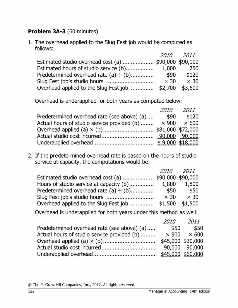
© The McGraw-Hill Companies, Inc., 2012. All rights reserved.
122 Managerial Accounting, 14th edition
Problem 3A-3 (60 minutes)
1. The overhead applied to the Slug Fest job would be computed as follows:
2010 2011 Estimated studio overhead cost (a) ................... $90,000 $90,000 Estimated hours of studio service (b) ................. 1,000 750 Predetermined overhead rate (a) ÷ (b) .............. $90 $120 Slug Fest job’s studio hours ............................. × 30 × 30 Overhead applied to the Slug Fest job .............. $2,700 $3,600
Overhead is underapplied for both years as computed below:
2010 2011 Predetermined overhead rate (see above) (a) .... $90 $120 Actual hours of studio service provided (b) ........ × 900 × 600 Overhead applied (a) × (b) ............................... $81,000 $72,000 Actual studio cost incurred ................................ 90,000 90,000 Underapplied overhead ..................................... $ 9,000 $18,000
2. If the predetermined overhead rate is based on the hours of studio
service at capacity, the computations would be:
2010 2011 Estimated studio overhead cost (a) ................... $90,000 $90,000 Hours of studio service at capacity (b) ............... 1,800 1,800 Predetermined overhead rate (a) ÷ (b) .............. $50 $50 Slug Fest job’s studio hours ............................. × 30 × 30 Overhead applied to the Slug Fest job .............. $1,500 $1,500
Overhead is underapplied for both years under this method as well:
2010 2011 Predetermined overhead rate (see above) (a) ....... $50 $50 Actual hours of studio service provided (b) ........... × 900 × 600 Overhead applied (a) × (b) .................................. $45,000 $30,000 Actual studio cost incurred ................................... 90,000 90,000 Underapplied overhead ........................................ $45,000 $60,000
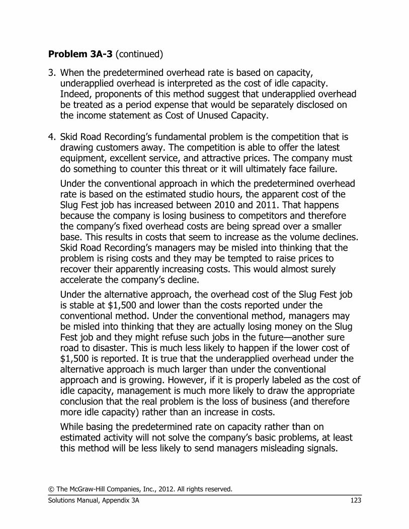
© The McGraw-Hill Companies, Inc., 2012. All rights reserved.
Solutions Manual, Appendix 3A 123
Problem 3A-3 (continued)
3. When the predetermined overhead rate is based on capacity, underapplied overhead is interpreted as the cost of idle capacity. Indeed, proponents of this method suggest that underapplied overhead be treated as a period expense that would be separately disclosed on the income statement as Cost of Unused Capacity.
4. Skid Road Recording’s fundamental problem is the competition that is
drawing customers away. The competition is able to offer the latest equipment, excellent service, and attractive prices. The company must do something to counter this threat or it will ultimately face failure.
Under the conventional approach in which the predetermined overhead rate is based on the estimated studio hours, the apparent cost of the Slug Fest job has increased between 2010 and 2011. That happens because the company is losing business to competitors and therefore the company’s fixed overhead costs are being spread over a smaller base. This results in costs that seem to increase as the volume declines. Skid Road Recording’s managers may be misled into thinking that the problem is rising costs and they may be tempted to raise prices to recover their apparently increasing costs. This would almost surely accelerate the company’s decline.
Under the alternative approach, the overhead cost of the Slug Fest job is stable at $1,500 and lower than the costs reported under the conventional method. Under the conventional method, managers may be misled into thinking that they are actually losing money on the Slug Fest job and they might refuse such jobs in the future—another sure road to disaster. This is much less likely to happen if the lower cost of $1,500 is reported. It is true that the underapplied overhead under the alternative approach is much larger than under the conventional approach and is growing. However, if it is properly labeled as the cost of idle capacity, management is much more likely to draw the appropriate conclusion that the real problem is the loss of business (and therefore more idle capacity) rather than an increase in costs.
While basing the predetermined rate on capacity rather than on estimated activity will not solve the company’s basic problems, at least this method will be less likely to send managers misleading signals.

© The McGraw-Hill Companies, Inc., 2012. All rights reserved.
124 Managerial Accounting, 14th edition
Case 3A-4 (120 minutes)
1. Traditional approach: Actual total manufacturing overhead cost incurred
(assumed to equal the original estimate) ................. $2,000,000 Manufacturing overhead applied
(80,000 units × $25 per unit) ................................. 2,000,000 Overhead underapplied or overapplied ....................... $ 0
TurboDrives, Inc.
Income Statement: Traditional Approach
Sales (75,000 units × $70 per unit) ............... $5,250,000 Cost of goods sold:
Variable manufacturing (75,000 units × $18 per unit) .................. $1,350,000
Manufacturing overhead applied (75,000 units × $25 per unit) .................. 1,875,000 3,225,000
Gross margin ............................................... 2,025,000 Selling and administrative expenses .............. 1,950,000 Net operating income ................................... $ 75,000
New approach: TurboDrives, Inc.
Income Statement: New Approach
Sales (75,000 units × $70 per unit) ............... $5,250,000 Cost of goods sold:
Variable manufacturing (75,000 units × $18 per unit) .................. $1,350,000
Manufacturing overhead applied (75,000 units × $20 per unit) .................. 1,500,000 2,850,000
Gross margin ............................................... 2,400,000 Cost of unused capacity [(100,000 units
80,000 units) × $20 per unit] ..................... 400,000 Selling and administrative expenses .............. 1,950,000 Net operating income ................................... $ 50,000

© The McGraw-Hill Companies, Inc., 2012. All rights reserved.
Solutions Manual, Appendix 3A 125
Case 3A-4 (continued)
2. Traditional approach: Under the traditional approach, the reported net operating income can
be increased by increasing the production level, which then results in overapplied overhead that is deducted from Cost of Goods Sold.
Additional net operating income required to attain target
net operating income ($210,000 − $75,000) (a) .......... $135,000 Overhead applied per unit of output (b) ......................... $25 per unit Additional output required to attain target net
operating income (a) ÷ (b) ......................................... 5,400 units Actual total manufacturing overhead cost incurred .......... $2,000,000 Manufacturing overhead applied
[(80,000 units + 5,400 units) × $25 per unit] .............. 2,135,000 Overhead overapplied ................................................... $ 135,000
TurboDrives, Inc.
Income Statement: Traditional Approach
Sales (75,000 units × $70 per unit) .............. $5,250,000 Cost of goods sold:
Variable manufacturing (75,000 units × $18 per unit) ................. $1,350,000
Manufacturing overhead applied (75,000 units × $25 per unit) ................. 1,875,000
Less: Manufacturing overhead overapplied . 135,000 3,090,000 Gross margin .............................................. 2,160,000 Selling and administrative expenses ............. 1,950,000 Net operating income .................................. $ 210,000
Note: If the overapplied manufacturing overhead were prorated
between ending inventories and Cost of Goods Sold, more units would have to be produced to attain the target net profit of $210,000.
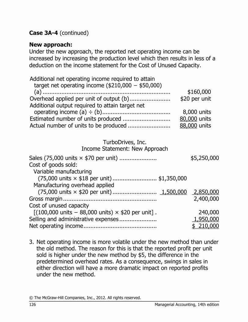
© The McGraw-Hill Companies, Inc., 2012. All rights reserved.
126 Managerial Accounting, 14th edition
Case 3A-4 (continued)
New approach: Under the new approach, the reported net operating income can be increased by increasing the production level which then results in less of a deduction on the income statement for the Cost of Unused Capacity. Additional net operating income required to attain
target net operating income ($210,000 − $50,000) (a) ........................................................................... $160,000
Overhead applied per unit of output (b) ........................ $20 per unit Additional output required to attain target net
operating income (a) ÷ (b) ........................................ 8,000 units Estimated number of units produced ............................ 80,000 units Actual number of units to be produced ......................... 88,000 units
TurboDrives, Inc.
Income Statement: New Approach
Sales (75,000 units × $70 per unit) ...................... $5,250,000 Cost of goods sold:
Variable manufacturing (75,000 units × $18 per unit) .......................... $1,350,000
Manufacturing overhead applied (75,000 units × $20 per unit) .......................... 1,500,000 2,850,000
Gross margin ....................................................... 2,400,000 Cost of unused capacity
[(100,000 units − 88,000 units) × $20 per unit] . 240,000 Selling and administrative expenses ...................... 1,950,000 Net operating income ........................................... $ 210,000
3. Net operating income is more volatile under the new method than under
the old method. The reason for this is that the reported profit per unit sold is higher under the new method by $5, the difference in the predetermined overhead rates. As a consequence, swings in sales in either direction will have a more dramatic impact on reported profits under the new method.

© The McGraw-Hill Companies, Inc., 2012. All rights reserved.
Solutions Manual, Appendix 3A 127
Case 3A-4 (continued)
4. As the computations in part (2) above show, the “hat trick” is a bit harder to perform under the new method. Under the old method, the target net operating income can be attained by producing an additional 5,400 units. Under the new method, the production would have to be increased by 8,000 units. This is a consequence of the difference in predetermined overhead rates. The drop in sales has had a more dramatic effect on net operating income under the new method as noted above in part (3). In addition, since the predetermined overhead rate is lower under the new method, producing excess inventories has less of an effect per unit on net operating income than under the traditional method and hence more excess production is required.
5. One can argue that whether the “hat trick” is unethical depends on the
level of sophistication of the owners of the company and others who read the financial statements. If they understand the effects of excess production on net operating income and are not misled, it can be argued that the hat trick is ethical. However, if that were the case, there does not seem to be any reason to use the hat trick. Why would the owners want to tie up working capital in inventories just to artificially attain a target net operating income for the period? And increasing the rate of production toward the end of the year is likely to increase overhead costs due to overtime and other costs. Building up inventories all at once is very likely to be much more expensive than increasing the rate of production uniformly throughout the year. In the case, we assumed that there would not be an increase in overhead costs due to the additional production, but that is likely not to be true.
In our opinion the hat trick is unethical unless there is a good reason for increasing production other than to artificially boost the current period’s net operating income. It is certainly unethical if the purpose is to fool users of financial reports such as owners and creditors or if the purpose is to meet targets so that bonuses will be paid to top managers.
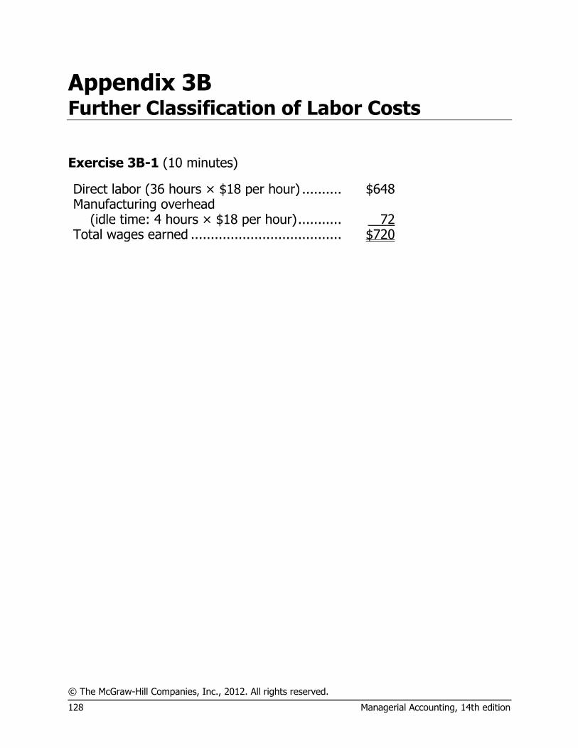
© The McGraw-Hill Companies, Inc., 2012. All rights reserved.
128 Managerial Accounting, 14th edition
Appendix 3B Further Classification of Labor Costs
Exercise 3B-1 (10 minutes)
Direct labor (36 hours × $18 per hour) .......... $648 Manufacturing overhead
(idle time: 4 hours × $18 per hour) ........... 72 Total wages earned ...................................... $720
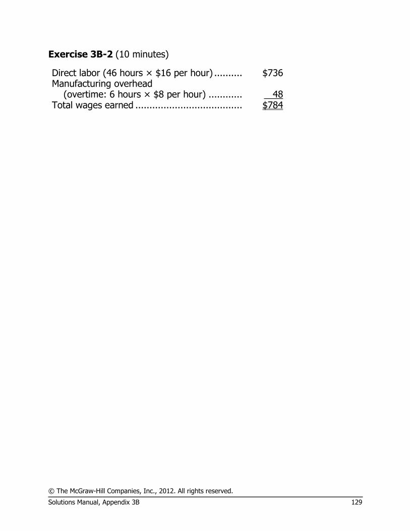
© The McGraw-Hill Companies, Inc., 2012. All rights reserved.
Solutions Manual, Appendix 3B 129
Exercise 3B-2 (10 minutes)
Direct labor (46 hours × $16 per hour) .......... $736 Manufacturing overhead
(overtime: 6 hours × $8 per hour) ............ 48 Total wages earned ...................................... $784

© The McGraw-Hill Companies, Inc., 2012. All rights reserved.
130 Managerial Accounting, 14th edition
Exercise 3B-3 (15 minutes)
1. No. It appears that the overtime spent completing the job was simply a matter of how the job happened to be scheduled. Under these circumstances, an overtime premium probably should not be charged to a customer whose job happens to fall at the tail end of the day’s schedule.
2. Direct labor: 9 hours × $20 per hour ................. $180 General overhead: 1 hour × $10 per hour ......... 10 Total labor cost ................................................ $190 3. A charge for an overtime premium might be justified if the customer
requested that the work be done on a “rush” basis.
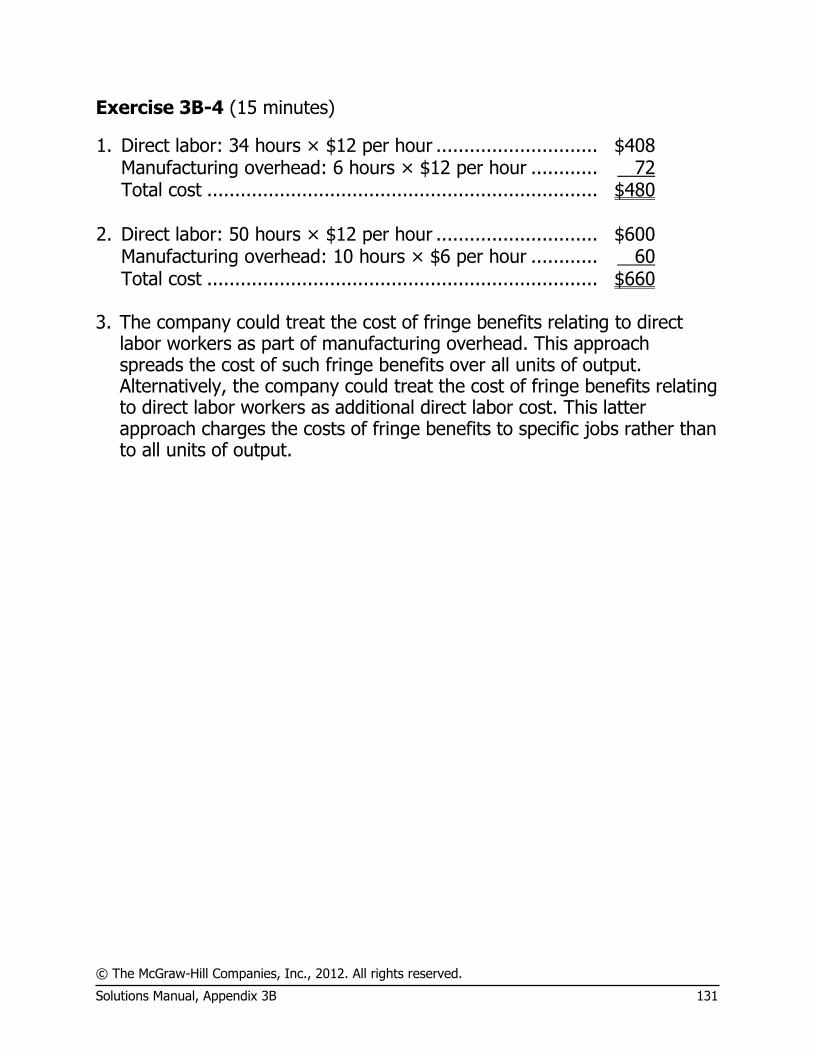
© The McGraw-Hill Companies, Inc., 2012. All rights reserved.
Solutions Manual, Appendix 3B 131
Exercise 3B-4 (15 minutes)
1. Direct labor: 34 hours × $12 per hour ............................. $408 Manufacturing overhead: 6 hours × $12 per hour ............ 72 Total cost ...................................................................... $480 2. Direct labor: 50 hours × $12 per hour ............................. $600 Manufacturing overhead: 10 hours × $6 per hour ............ 60 Total cost ...................................................................... $660 3. The company could treat the cost of fringe benefits relating to direct
labor workers as part of manufacturing overhead. This approach spreads the cost of such fringe benefits over all units of output. Alternatively, the company could treat the cost of fringe benefits relating to direct labor workers as additional direct labor cost. This latter approach charges the costs of fringe benefits to specific jobs rather than to all units of output.

© The McGraw-Hill Companies, Inc., 2012. All rights reserved.
132 Managerial Accounting, 14th edition
Problem 3B-5 (30 minutes)
1. Total wages for the week: Regular time: 40 hours × $24 per hour .................. $ 960 Overtime: 5 hours × $36 per hour ......................... 180 Total wages ............................................................ $1,140 Allocation of total wages: Direct labor: 45 hours × $24 per hour .................... $1,080 Manufacturing overhead: 5 hours × $12 per hour ... 60 Total wages ............................................................ $1,140 2. Total wages for the week: Regular time: 40 hours × $24 per hour .................. $ 960 Overtime: 10 hours × $36 per hour ....................... 360 Total wages ............................................................ $1,320 Allocation of total wages: Direct labor: 46 hours × $24 per hour .................... $1,104 Manufacturing overhead: Idle time: 4 hours × $24 per hour ....................... $ 96 Overtime premium: 10 hours × $12 per hour....... 120 216 Total wages ............................................................ $1,320
3. Total wages and fringe benefits for the week: Regular time: 40 hours × $24 per hour .................. $ 960 Overtime: 8 hours × $36 per hour ......................... 288 Fringe benefits: 48 hours × $8 per hour ................. 384 Total wages and fringe benefits ............................... $1,632 Allocation of wages and fringe benefits: Direct labor: 45 hours × $24 per hour .................... $1,080 Manufacturing overhead: Idle time: 3 hours × $24 per hour ....................... $ 72 Overtime premium: 8 hours × $12 per hour ........ 96 Fringe benefits: 48 hours × $8 per hour .............. 384 552 Total wages and fringe benefits ............................... $1,632

© The McGraw-Hill Companies, Inc., 2012. All rights reserved.
Solutions Manual, Appendix 3B 133
Problem 3B-5 (continued)
4. Allocation of wages and fringe benefits: Direct labor: Wage cost: 45 hours × $24 per hour ................ $1,080 Fringe benefits: 45 hours × $8 per hour ........... 360 $1,440 Manufacturing overhead: Idle time: 3 hours × $24 per hour .................... 72 Overtime premium: 8 hours × $12 per hour ..... 96 Fringe benefits: 3 hours × $8 per hour ............. 24 192 Total wages and fringe benefits .......................... $1,632

© The McGraw-Hill Companies, Inc., 2012. All rights reserved.
Solutions Manual, Chapter 4 135
Chapter 4 Process Costing
Solutions to Questions
4-1 A process costing system should be used in situations where a homogeneous product is produced on a continuous basis.
4-2 Job-order and processing costing are similar in the following ways: 1. Job-order costing and process costing have
the same basic purposes—to assign materials, labor, and overhead cost to products and to provide a mechanism for computing unit product costs.
2. Both systems use the same basic manufacturing accounts.
3. Costs flow through the accounts in basically the same way in both systems.
4-3 Cost accumulation is simpler under process costing because costs only need to be assigned to departments—not individual jobs. A company usually has a small number of processing departments, whereas a job-order costing system often must keep track of the costs of hundreds or even thousands of jobs.
4-4 In a process costing system, a Work in Process account is maintained for each processing department.
4-5 The journal entry to record the transfer of work in process from the Mixing Department to the Firing Department is:
Work in Process, Firing ..................................... XXXX Work in Process, Mixing.............................. XXXX
4-6 The costs that might be added in the Firing Department include: (1) costs transferred in from the Mixing Department; (2) materials costs added in the Firing Department; (3) labor costs added in the Firing Department; and (4) overhead costs added in the Firing Department.
4-7 Under the weighted-average method, equivalent units of production consist of units transferred to the next department (or to finished goods) during the period plus the equivalent units in the department’s ending work in process inventory.
4-8 The company will want to distinguish between the costs of the metals used to make the medallions, but the medals are otherwise identical and go through the same production processes. Thus, operation costing is ideally suited for the company’s needs.

© The McGraw-Hill Companies, Inc., 2012. All rights reserved.
136 Managerial Accounting, 14th Edition
Exercise 4-1 (20 minutes)
a. To record issuing raw materials for use in production: Work in Process—Molding Department ......... 28,000 Work in Process—Firing Department ............ 5,000 Raw Materials ...................................... 33,000 b. To record direct labor costs incurred: Work in Process—Molding Department ......... 18,000 Work in Process—Firing Department ............ 5,000 Wages Payable..................................... 23,000 c. To record applying manufacturing overhead: Work in Process—Molding Department ......... 24,000 Work in Process—Firing Department ............ 37,000 Manufacturing Overhead....................... 61,000 d. To record transfer of unfired, molded bricks from the Molding
Department to the Firing Department: Work in Process—Firing Department ............ 67,000 Work in Process—Molding Department... 67,000 e. To record transfer of finished bricks from the Firing Department to the
finished goods warehouse: Finished Goods ........................................... 108,000 Work in Process—Firing Department ...... 108,000 f. To record Cost of Goods Sold: Cost of Goods Sold...................................... 106,000 Finished Goods..................................... 106,000

© The McGraw-Hill Companies, Inc., 2012. All rights reserved.
Solutions Manual, Chapter 4 137
Exercise 4-2 (10 minutes)
Weighted-Average Method
Equivalent Units Materials Conversion Units transferred out ................................... 410,000 410,000 Work in process, ending:
30,000 units × 70%................................... 21,000 30,000 units × 50%................................... 15,000
Equivalent units of production ....................... 431,000 425,000
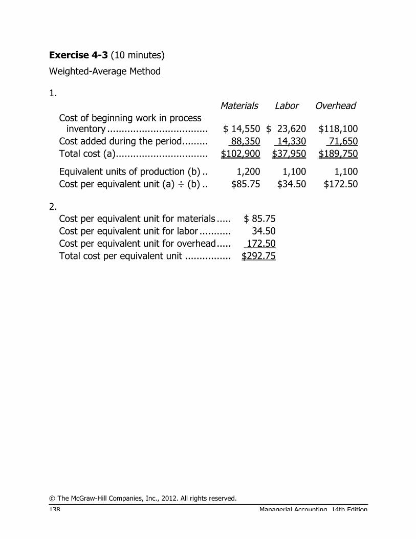
© The McGraw-Hill Companies, Inc., 2012. All rights reserved.
138 Managerial Accounting, 14th Edition
Exercise 4-3 (10 minutes)
Weighted-Average Method 1.
Materials Labor Overhead Cost of beginning work in process
inventory ................................... $ 14,550 $ 23,620 $118,100 Cost added during the period......... 88,350 14,330 71,650 Total cost (a)................................ $102,900 $37,950 $189,750
Equivalent units of production (b) .. 1,200 1,100 1,100 Cost per equivalent unit (a) ÷ (b) .. $85.75 $34.50 $172.50
2.
Cost per equivalent unit for materials ..... $ 85.75 Cost per equivalent unit for labor ........... 34.50 Cost per equivalent unit for overhead..... 172.50 Total cost per equivalent unit ................ $292.75
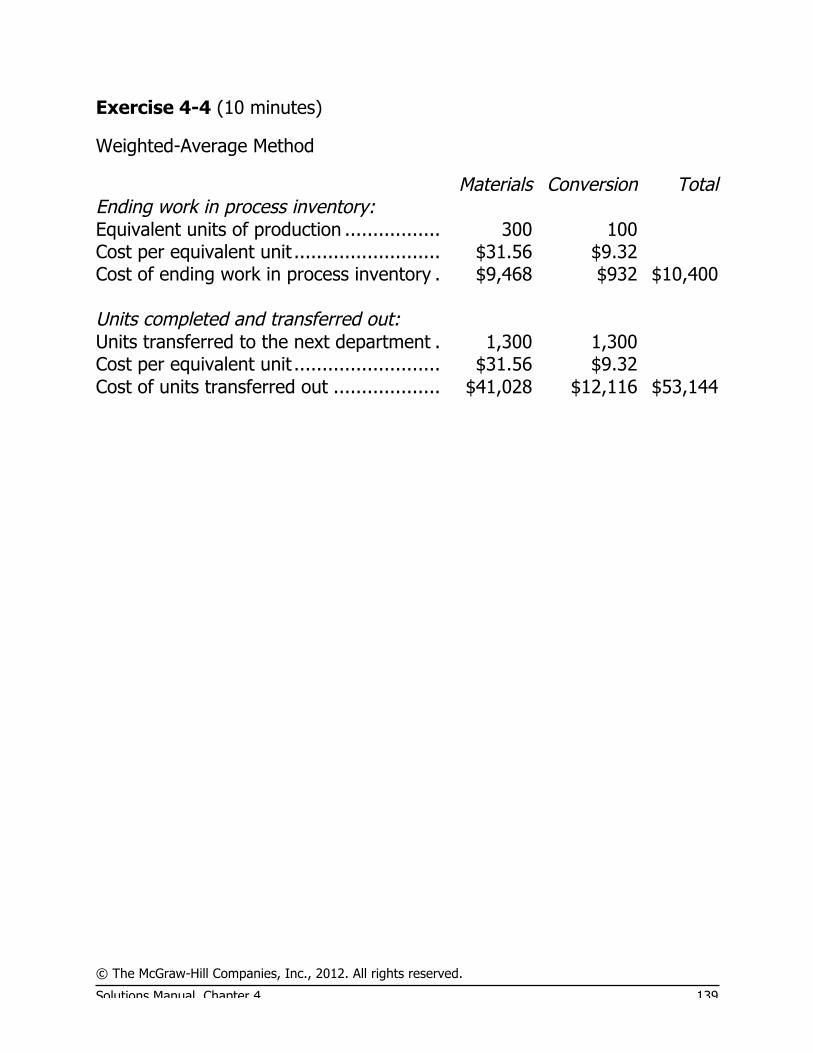
© The McGraw-Hill Companies, Inc., 2012. All rights reserved.
Solutions Manual, Chapter 4 139
Exercise 4-4 (10 minutes)
Weighted-Average Method
Materials Conversion Total Ending work in process inventory: Equivalent units of production ................. 300 100 Cost per equivalent unit .......................... $31.56 $9.32 Cost of ending work in process inventory . $9,468 $932 $10,400 Units completed and transferred out: Units transferred to the next department . 1,300 1,300 Cost per equivalent unit .......................... $31.56 $9.32 Cost of units transferred out ................... $41,028 $12,116 $53,144
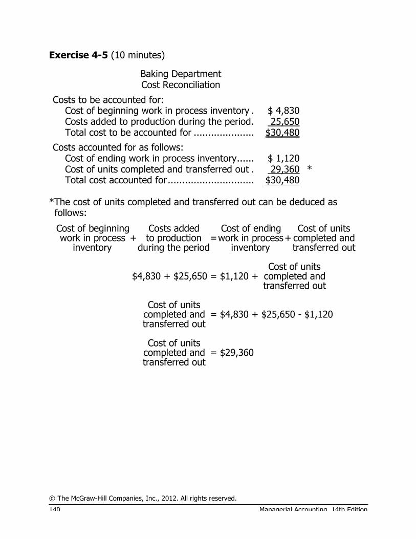
© The McGraw-Hill Companies, Inc., 2012. All rights reserved.
140 Managerial Accounting, 14th Edition
Exercise 4-5 (10 minutes)
Baking Department Cost Reconciliation
Costs to be accounted for: Cost of beginning work in process inventory . $ 4,830 Costs added to production during the period. 25,650 Total cost to be accounted for ..................... $30,480
Costs accounted for as follows: Cost of ending work in process inventory...... $ 1,120 Cost of units completed and transferred out . 29,360 * Total cost accounted for.............................. $30,480
*The cost of units completed and transferred out can be deduced as follows:

© The McGraw-Hill Companies, Inc., 2012. All rights reserved.
Solutions Manual, Chapter 4 141
Exercise 4-6 (15 minutes)
Weighted-Average Method 1. Materials Labor Overhead Units transferred to the next
department ..................................... 790,000 790,000 790,000 Work in process, ending:
Materials: 50,000 units × 60% complete........ 30,000
Labor and overhead: 50,000 units × 20% complete........ 10,000 10,000
Equivalent units of production ............. 820,000 800,000 800,000 2. Materials Labor Overhead Cost of beginning work in process.... $ 68,600 $ 30,000 $ 48,000 Cost added during the period........... 907,200 370,000 592,000
Total cost (a).................................. $975,800 $400,00
0 $640,000
Equivalent units of production (b) .... 820,000 800,000 800,000 Cost per equivalent unit (a) ÷ (b) .... $1.19 $0.50 $0.80
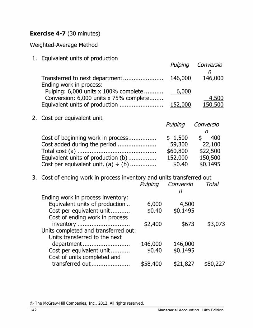
© The McGraw-Hill Companies, Inc., 2012. All rights reserved.
142 Managerial Accounting, 14th Edition
Exercise 4-7 (30 minutes)
Weighted-Average Method 1. Equivalent units of production Pulping Conversio
n Transferred to next department ....................... 146,000 146,000 Ending work in process: Pulping: 6,000 units x 100% complete ........... 6,000 Conversion: 6,000 units x 75% complete........ 4,500 Equivalent units of production ......................... 152,000 150,500
2. Cost per equivalent unit Pulping Conversio
n Cost of beginning work in process................ $ 1,500 $ 400 Cost added during the period ...................... 59,300 22,100 Total cost (a) ............................................. $60,800 $22,500 Equivalent units of production (b) ................ 152,000 150,500 Cost per equivalent unit, (a) ÷ (b) ............... $0.40 $0.1495
3. Cost of ending work in process inventory and units transferred out Pulping Conversio
n Total
Ending work in process inventory: Equivalent units of production .. 6,000 4,500 Cost per equivalent unit ........... $0.40 $0.1495 Cost of ending work in process
inventory .............................. $2,400 $673 $3,073 Units completed and transferred out: Units transferred to the next
department ........................... 146,000 146,000 Cost per equivalent unit ........... $0.40 $0.1495 Cost of units completed and
transferred out ...................... $58,400 $21,827 $80,227

© The McGraw-Hill Companies, Inc., 2012. All rights reserved.
Solutions Manual, Chapter 4 143
Exercise 4-7 (continued)
4.
Cost reconciliation
Costs to be accounted for: Cost of beginning work in process inventory
($1,500 + $400)........................................ $ 1,900 Costs added to production during the period
($59,300 + $22,100) ................................. 81,400 Total cost to be accounted for ...................... $83,300 Costs accounted for as follows: Cost of ending work in process inventory ...... $ 3,073 Cost of units completed and transferred out .. 80,227 Total cost accounted for............................... $83,300

© The McGraw-Hill Companies, Inc., 2012. All rights reserved.
144 Managerial Accounting, 14th Edition
Exercise 4-8 (10 minutes)
Work in Process—Mixing................................................ 330,000 Raw Materials Inventory ........................................... 330,000
Work in Process—Mixing................................................ 260,000 Work in Process—Baking ............................................... 120,000
Wages Payable ........................................................ 380,000
Work in Process—Mixing................................................ 190,000 Work in Process—Baking ............................................... 90,000
Manufacturing Overhead .......................................... 280,000
Work in Process—Baking ............................................... 760,000 Work in Process—Mixing........................................... 760,000
Finished Goods ............................................................. 980,000 Work in Process—Baking .......................................... 980,000
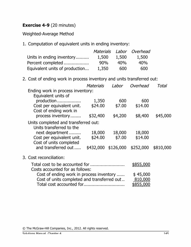
© The McGraw-Hill Companies, Inc., 2012. All rights reserved.
Solutions Manual, Chapter 4 145
Exercise 4-9 (20 minutes)
Weighted-Average Method 1. Computation of equivalent units in ending inventory:
Materials Labor Overhead Units in ending inventory.......... 1,500 1,500 1,500 Percent completed ................... 90% 40% 40% Equivalent units of production... 1,350 600 600
2. Cost of ending work in process inventory and units transferred out:
Materials Labor Overhead Total Ending work in process inventory: Equivalent units of
production .................. 1,350 600 600 Cost per equivalent unit. $24.00 $7.00 $14.00 Cost of ending work in
process inventory........ $32,400 $4,200 $8,400 $45,000
Units completed and transferred out: Units transferred to the
next department ......... 18,000 18,000 18,000 Cost per equivalent unit. $24.00 $7.00 $14.00 Cost of units completed
and transferred out ..... $432,000 $126,000 $252,000 $810,000 3. Cost reconciliation:
Total cost to be accounted for .......................... $855,000 Costs accounted for as follows: Cost of ending work in process inventory ...... $ 45,000 Cost of units completed and transferred out .. 810,000 Total cost accounted for............................... $855,000

© The McGraw-Hill Companies, Inc., 2012. All rights reserved.
146 Managerial Accounting, 14th Edition
Exercise 4-10 (10 minutes)
Weighted-Average Method
1. Kilograms of
Cement Work in process, May 1........................................... 80,000 Started into production during the month................. 300,000 Total kilograms in process ....................................... 380,000 Deduct work in process, May 31 .............................. 50,000 Completed and transferred out during the month...... 330,000
2. Equivalent Units (EU) Materials Conversion Units transferred out................................ 330,000 330,000 Work in process, ending: Materials: 50,000 kilograms × 40%........ 20,000 Conversion: 50,000 kilograms × 10%..... 5,000 Equivalent units of production .................. 350,000 335,000

© The McGraw-Hill Companies, Inc., 2012. All rights reserved.
Solutions Manual, Chapter 4 147
Exercise 4-11 (30 minutes)
Weighted-Average Method
1. Material
s Conversio
n Units transferred to the next process............... 300,000 300,000 Ending work in process: Materials: 40,000 units × 50% complete ....... 20,000 Conversion: 40,000 units × 25% complete.... 10,000 Equivalent units of production......................... 320,000 310,000
2.
Material
s Conversio
n Cost of beginning work in process .................. $ 56,600 $ 14,900 Cost added during the period......................... 385,000 214,500
Total cost (a)................................................ $441,60
0 $229,400 Equivalent units of production (b) .................. 320,000 310,000 Cost per equivalent unit (a) ÷ (b) .................. $1.38 $0.74 3. Materials Conversion Total Ending work in process inventory: Equivalent units of production
(see above)........................ 20,000 10,000 Cost per equivalent unit (see
above)............................... $1.38 $0.74 Cost of ending work in process
inventory ........................... $27,600 $7,400 $35,000 Units completed and transferred out: Units transferred to the next
process.............................. 300,000 300,000 Cost per equivalent unit
(see previous exercise) ....... $1.38 $0.74 Cost of units completed and
transferred out ................... $414,000 $222,000 $636,000

© The McGraw-Hill Companies, Inc., 2012. All rights reserved.
148 Managerial Accounting, 14th Edition
Exercise 4-12 (10 minutes)
Weighted-Average Method
Material
s Labor &
Overhead Pounds transferred to the Packing Department
during May* ....................................................... 490,000 490,000 Work in process, May 31:
Materials: 20,000 pounds × 100% complete......... 20,000 Labor and overhead: 20,000 pounds × 90%
complete ......................................................... 18,000 Equivalent units of production ................................ 510,000 508,000
* 30,000 + 480,000 – 20,000 = 490,000

© The McGraw-Hill Companies, Inc., 2012. All rights reserved.
Solutions Manual, Chapter 4 149
Problem 4-13 (45 minutes)
Weighted-Average Method 1. Equivalent Units of Production Materials Conversio
n Transferred to next department* ..................... 380,000 380,000 Ending work in process: Materials: 40,000 units x 75% complete......... 30,000 Conversion: 40,000 units x 25% complete...... 10,000 Equivalent units of production ......................... 410,000 390,000
*Units transferred to the next department = Units in beginning work in process + Units started into production − Units in ending work in process = 70,000 + 350,000 − 40,000 = 380,000
2. Cost per Equivalent Unit Materials Conversio
n Cost of beginning work in process................ $ 86,000 $ 36,000 Cost added during the period ...................... 447,000 198,000 Total cost (a) ............................................. $533,000 $234,000 Equivalent units of production (b) ................ 410,000 390,000 Cost per equivalent unit, (a) ÷ (b) ............... $1.30 $0.60
3. Cost of Ending Work in Process Inventory and Units Transferred Out Materials Conversio
n Total
Ending work in process inventory: Equivalent units of production
(materials: 40,000 units x 75% complete; conversion: 40,000 units x 25% complete)....... 30,000 10,000
Cost per equivalent unit ....... $1.30 $0.60 Cost of ending work in process
inventory .......................... $39,000 $6,000 $45,000 Units completed and transferred out: Units transferred to the next
department ....................... 380,000 380,000 Cost per equivalent unit ....... $1.30 $0.60

© The McGraw-Hill Companies, Inc., 2012. All rights reserved.
150 Managerial Accounting, 14th Edition
Cost of units completed and transferred out .................. $494,000 $228,000 $722,000

© The McGraw-Hill Companies, Inc., 2012. All rights reserved.
Solutions Manual, Chapter 4 151
Problem 4-13 (continued)
4.
Cost Reconciliation
Costs to be accounted for: Cost of beginning work in process inventory
($86,000 + $36,000) ................................. $122,000 Costs added to production during the period
($447,000 + $198,000).............................. 645,000 Total cost to be accounted for ...................... $767,000 Costs accounted for as follows: Cost of ending work in process inventory ...... $ 45,000 Cost of units completed and transferred out .. 722,000 Total cost accounted for............................... $767,000

© The McGraw-Hill Companies, Inc., 2012. All rights reserved.
152 Managerial Accounting, 14th Edition
Problem 4-14 (45 minutes)
Weighted-Average Method 1. Equivalent Units of Production Materials Conversio
n Transferred to next department ....................... 450,000 450,000 Ending work in process: Materials: 80,000 units x 75% complete......... 60,000 Conversion: 80,000 units x 25% complete...... 20,000 Equivalent units of production ......................... 510,000 470,000
2. Cost per Equivalent Unit Materials Conversio
n Cost of beginning work in process................ $ 36,550 $ 13,500 Cost added during the period ...................... 391,850 287,300 Total cost (a) ............................................. $428,400 $300,800 Equivalent units of production (b) ................ 510,000 470,000 Cost per equivalent unit, (a) ÷ (b) ............... $0.84 $0.64
3. Applying Costs to Units Materials Conversio
n Total
Ending work in process inventory: Equivalent units of production 60,000 20,000 Cost per equivalent unit ....... $0.84 $0.64 Cost of ending work in process
inventory .......................... $50,400 $12,800 $63,200 Units completed and transferred out: Units transferred to the next
department ....................... 450,000 450,000 Cost per equivalent unit ....... $0.84 $0.64 Cost of units completed and
transferred out .................. $378,000 $288,000 $666,000

© The McGraw-Hill Companies, Inc., 2012. All rights reserved.
Solutions Manual, Chapter 4 153
Problem 4-14 (continued)
4.
Cost Reconciliation
Costs to be accounted for: Cost of beginning work in process inventory
($36,550 + $13,500) ................................. $ 50,050 Costs added to production during the period
($391,850 + $287,300).............................. 679,150 Total cost to be accounted for ...................... $729,200 Costs accounted for as follows: Cost of ending work in process inventory ...... $ 63,200 Cost of units completed and transferred out .. 666,000 Total cost accounted for............................... $729,200


© The McGraw-Hill Companies, Inc., 2012. All rights reserved.
Solutions Manual, Chapter 4 155
Problem 4-15 (45 minutes)
Weighted-Average Method 1. Equivalent units of production Materials Conversio
n Transferred to next department* ..................... 270,000 270,000 Ending work in process: Materials: 45,000 units x 100% complete ....... 45,000 Conversion: 45,000 units x 60% complete...... 27,000 Equivalent units of production ......................... 315,000 297,000
*Units transferred to the next department = Units in beginning work in process + Units started into production − Units in ending work in process = 35,000 + 280,000 − 45,000 = 270,000
2. Cost per equivalent unit Materials Conversio
n Cost of beginning work in process................ $ 43,400 $ 20,300 Cost added during the period ...................... 397,600 187,600 Total cost (a) ............................................. $441,000 $207,900 Equivalent units of production (b) ................ 315,000 297,000 Cost per equivalent unit, (a) ÷ (b) ............... $1.40 $0.70
3. Cost of ending work in process inventory and units transferred out Materials Conversio
n Total
Ending work in process inventory: Equivalent units of production .. 45,000 27,000 Cost per equivalent unit ........... $1.40 $0.70 Cost of ending work in process
inventory .............................. $63,000 $18,900 $81,900 Units completed and transferred out: Units transferred to the next
department ........................... 270,000 270,000 Cost per equivalent unit ........... $1.40 $0.70 Cost of units completed and
transferred out ...................... $378,000 $189,000 $567,000

© The McGraw-Hill Companies, Inc., 2012. All rights reserved.
156 Managerial Accounting, 14th Edition
Problem 4-16 (45 minutes)
Weighted-Average Method 1. a. Work in Process—Blending ............................................. 147,600 Work in Process—Bottling............................................... 45,000 Raw Materials........................................................... 192,600
b. Work in Process—Blending ............................................. 73,200 Work in Process—Bottling............................................... 17,000 Salaries and Wages Payable ...................................... 90,200
c. Manufacturing Overhead ................................................ 596,000 Accounts Payable ..................................................... 596,000
d. Work in Process—Blending ............................................. 481,000 Manufacturing Overhead ........................................... 481,000 Work in Process—Bottling............................................... 108,000 Manufacturing Overhead ........................................... 108,000
e. Work in Process—Bottling............................................... 722,000 Work in Process—Blending ........................................ 722,000
f. Finished Goods.............................................................. 920,000 Work in Process—Bottling ......................................... 920,000
g. Accounts Receivable ...................................................... 1,400,000 Sales ....................................................................... 1,400,000 Cost of Goods Sold ........................................................ 890,000 Finished Goods......................................................... 890,000

© The McGraw-Hill Companies, Inc., 2012. All rights reserved.
Solutions Manual, Chapter 4 157
Problem 4-16 (continued)
2.
Accounts Receivable Raw Materials (g) 1,400,000 Bal. 198,600 (a) 192,600 Bal. 6,000
Work in Process
Blending Department Work in Process
Bottling Department Bal. 32,800 (e) 722,000 Bal. 49,000 (f) 920,000 (a) 147,600 (a) 45,000 (b) 73,200 (b) 17,000 (d) 481,000 (d) 108,000 Bal. 12,600 (e) 722,000 Bal. 21,000
Finished Goods Manufacturing Overhead
Bal. 20,000 (g) 890,000 (c) 596,000 (d) 589,000 (f) 920,000 Bal. 7,000 Bal. 50,000
Accounts Payable Salaries and Wages Payable
(c) 596,000 (b) 90,200
Sales Cost of Goods Sold (g) 1,400,000 (g) 890,000
© The McGraw-Hill Companies, Inc., 2012. All rights reserved.
Solutions Manual, Chapter 5 193
Chapter 5 Cost-Volume-Profit Relationships
Solutions to Questions
5-1 The contribution margin (CM) ratio is the ratio of the total contribution margin to total sales revenue. It is used in target profit and break-even analysis and can be used to quickly estimate the effect on profits of a change in sales revenue.
5-2 Incremental analysis focuses on the changes in revenues and costs that will result from a particular action.
5-3 All other things equal, Company B, with its higher fixed costs and lower variable costs, will have a higher contribution margin ratio than Company A. Therefore, it will tend to realize a larger increase in contribution margin and in profits when sales increase.
5-4 Operating leverage measures the impact on net operating income of a given percentage change in sales. The degree of operating leverage at a given level of sales is computed by dividing the contribution margin at that level of sales by the net operating income at that level of sales.
5-5 The break-even point is the level of sales at which profits are zero.
5-6 (a) If the selling price decreased, then the total revenue line would rise less steeply, and the break-even point would occur at a higher unit volume. (b) If the fixed cost
increased, then both the fixed cost line and the total cost line would shift upward and the break-even point would occur at a higher unit volume. (c) If the variable cost increased, then the total cost line would rise more steeply and the break-even point would occur at a higher unit volume.
5-7 The margin of safety is the excess of budgeted (or actual) sales over the break-even volume of sales. It is the amount by which sales can drop before losses begin to be incurred.
5-8 The sales mix is the relative proportions in which a company’s products are sold. The usual assumption in cost-volume-profit analysis is that the sales mix will not change.
5-9 A higher break-even point and a lower net operating income could result if the sales mix shifted from high contribution margin products to low contribution margin products. Such a shift would cause the average contribution margin ratio in the company to decline, resulting in less total contribution margin for a given amount of sales. Thus, net operating income would decline. With a lower contribution margin ratio, the break-even point would be higher because more sales would be required to cover the same amount of fixed costs.
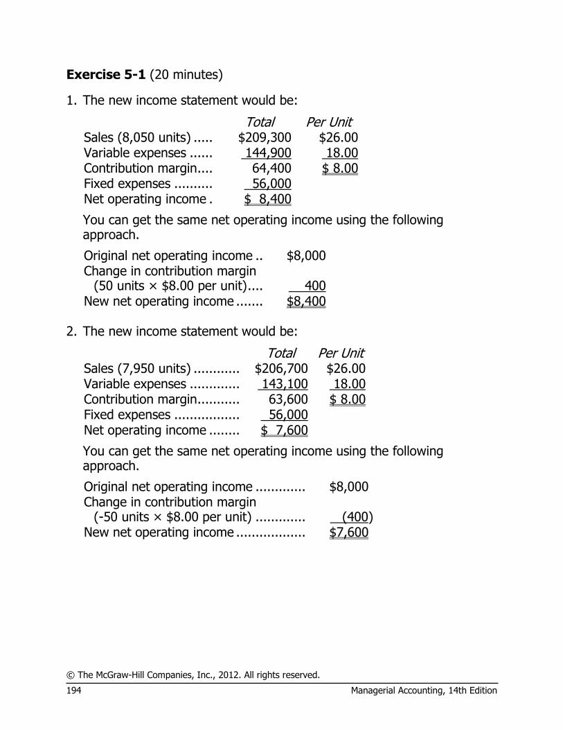
© The McGraw-Hill Companies, Inc., 2012. All rights reserved.
194 Managerial Accounting, 14th Edition
Exercise 5-1 (20 minutes)
1. The new income statement would be:
Total Per Unit Sales (8,050 units) ..... $209,300 $26.00 Variable expenses ...... 144,900 18.00 Contribution margin .... 64,400 $ 8.00 Fixed expenses .......... 56,000 Net operating income . $ 8,400
You can get the same net operating income using the following approach.
Original net operating income .. $8,000 Change in contribution margin
(50 units × $8.00 per unit) .... 400 New net operating income ....... $8,400 2. The new income statement would be:
Total Per Unit Sales (7,950 units) ............ $206,700 $26.00 Variable expenses ............. 143,100 18.00 Contribution margin ........... 63,600 $ 8.00 Fixed expenses ................. 56,000 Net operating income ........ $ 7,600
You can get the same net operating income using the following approach.
Original net operating income ............. $8,000
Change in contribution margin
(-50 units × $8.00 per unit) ............. (400) New net operating income .................. $7,600

© The McGraw-Hill Companies, Inc., 2012. All rights reserved.
Solutions Manual, Chapter 5 195
Exercise 5-1 (continued)
3. The new income statement would be:
Total Per Unit Sales (7,000 units) ....... $182,000 $26.00 Variable expenses ........ 126,000 18.00 Contribution margin ...... 56,000 $ 8.00 Fixed expenses ............ 56,000 Net operating income ... $ 0
Note: This is the company's break-even point.
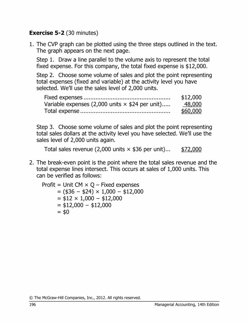
© The McGraw-Hill Companies, Inc., 2012. All rights reserved.
196 Managerial Accounting, 14th Edition
Exercise 5-2 (30 minutes)
1. The CVP graph can be plotted using the three steps outlined in the text. The graph appears on the next page.
Step 1. Draw a line parallel to the volume axis to represent the total fixed expense. For this company, the total fixed expense is $12,000.
Step 2. Choose some volume of sales and plot the point representing total expenses (fixed and variable) at the activity level you have selected. We’ll use the sales level of 2,000 units.
Fixed expenses ................................................... $12,000 Variable expenses (2,000 units × $24 per unit) ..... 48,000 Total expense ..................................................... $60,000
Step 3. Choose some volume of sales and plot the point representing
total sales dollars at the activity level you have selected. We’ll use the sales level of 2,000 units again.
Total sales revenue (2,000 units × $36 per unit) ... $72,000 2. The break-even point is the point where the total sales revenue and the
total expense lines intersect. This occurs at sales of 1,000 units. This can be verified as follows:
Profit = Unit CM × Q – Fixed expenses = ($36 − $24) × 1,000 − $12,000 = $12 × 1,000 − $12,000 = $12,000 − $12,000 = $0
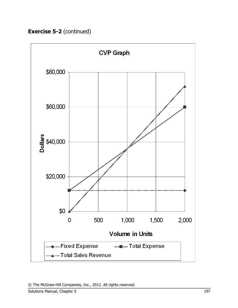
© The McGraw-Hill Companies, Inc., 2012. All rights reserved.
Solutions Manual, Chapter 5 197
Exercise 5-2 (continued)

© The McGraw-Hill Companies, Inc., 2012. All rights reserved.
198 Managerial Accounting, 14th Edition
Exercise 5-3 (15 minutes)
1. The profit graph is based on the following simple equation:
Profit = Unit CM × Q − Fixed expenses Profit = ($19 − $15) × Q − $12,000 Profit = $4 × Q − $12,000
To plot the graph, select two different levels of sales such as Q=0 and Q=4,000. The profit at these two levels of sales are -$12,000 (= $4 × 0 − $12,000) and $4,000 (= $4 × 4,000 − $12,000).
Profit Graph
-$20,000
-$15,000
-$10,000
-$5,000
$0
$5,000
0 500 1,000 1,500 2,000 2,500 3,000 3,500 4,000
Sales Volume in Units
Pro
fit

© The McGraw-Hill Companies, Inc., 2012. All rights reserved.
Solutions Manual, Chapter 5 199
Exercise 5-3 (continued)
2. Looking at the graph, the break-even point appears to be 3,000 units. This can be verified as follows:
Profit = Unit CM × Q − Fixed expenses = $4 × Q − $12,000 = $4 × 3,000 − $12,000 = $12,000 − $12,000 = $0

© The McGraw-Hill Companies, Inc., 2012. All rights reserved.
200 Managerial Accounting, 14th Edition
Exercise 5-4 (10 minutes)
1. The company’s contribution margin (CM) ratio is:
Total sales ............................ $300,000 Total variable expenses ......... 240,000 = Total contribution margin ... $ 60,000 ÷ Total sales ......................... $300,000 = CM ratio ............................ 20%
2. The change in net operating income from an increase in total sales of
$1,500 can be estimated by using the CM ratio as follows:
Change in total sales ...................... $1,500 × CM ratio ..................................... 20%
= Estimated change in net
operating income ......................... $ 300
This computation can be verified as follows:
Total sales ................... $300,000 ÷ Total units sold ......... 40,000 units = Selling price per unit . $7.50 per unit Increase in total sales ... $1,500 ÷ Selling price per unit . $7.50 per unit = Increase in unit sales 200 units Original total unit sales . 40,000 units New total unit sales ...... 40,200 units
Original New Total unit sales............. 40,000 40,200 Sales ........................... $300,000 $301,500 Variable expenses ........ 240,000 241,200 Contribution margin ...... 60,000 60,300 Fixed expenses ............ 45,000 45,000 Net operating income ... $ 15,000 $ 15,300

© The McGraw-Hill Companies, Inc., 2012. All rights reserved.
Solutions Manual, Chapter 5 201
Exercise 5-5 (20 minutes)
1. The following table shows the effect of the proposed change in monthly advertising budget:
Sales With Additional Current Advertising Sales Budget Difference Sales ........................... $225,000 $240,000 $15,000 Variable expenses ........ 135,000 144,000 9,000 Contribution margin ...... 90,000 96,000 6,000 Fixed expenses ............ 75,000 83,000 8,000 Net operating income ... $ 15,000 $ 13,000 $(2,000)
Assuming that there are no other important factors to be considered, the increase in the advertising budget should not be approved because it would lead to a decrease in net operating income of $2,000.
Alternative Solution 1
Expected total contribution margin:
$240,000 × 40% CM ratio .................. $96,000
Present total contribution margin:
$225,000 × 40% CM ratio .................. 90,000 Incremental contribution margin ........... 6,000
Change in fixed expenses:
Less incremental advertising expense . 8,000 Change in net operating income ............ $(2,000)
Alternative Solution 2
Incremental contribution margin:
$15,000 × 40% CM ratio ................... $6,000 Less incremental advertising expense .... 8,000 Change in net operating income ............ $(2,000)
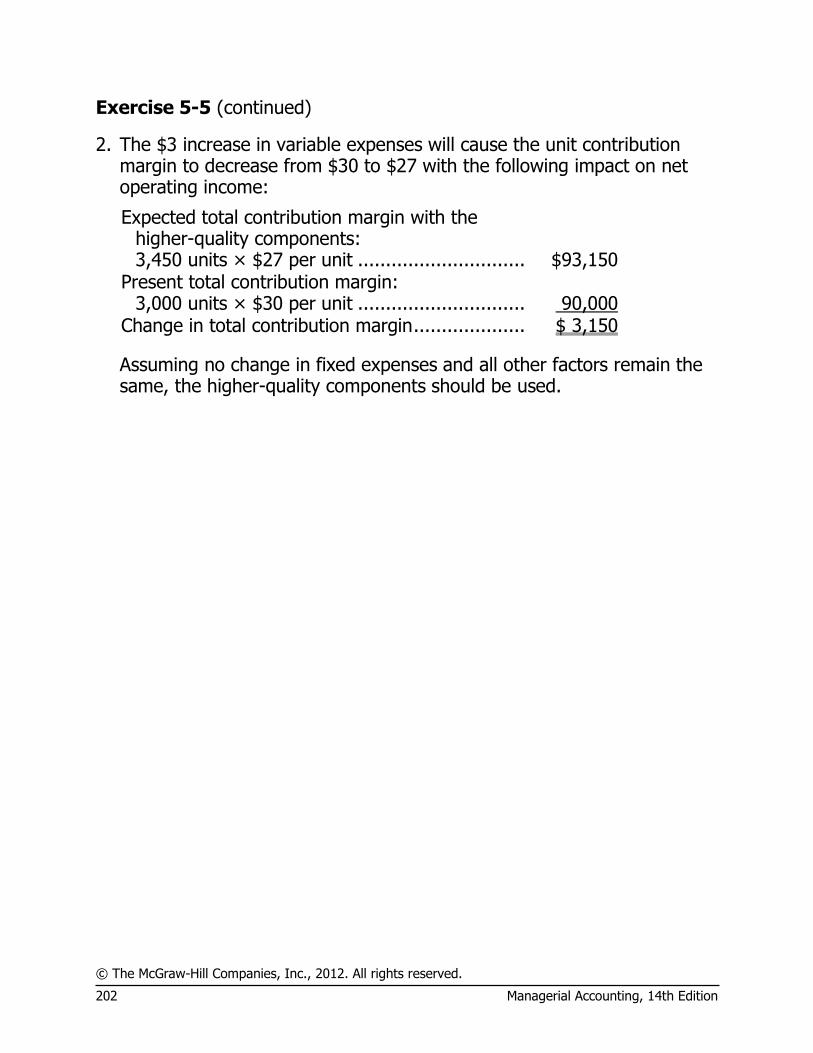
© The McGraw-Hill Companies, Inc., 2012. All rights reserved.
202 Managerial Accounting, 14th Edition
Exercise 5-5 (continued)
2. The $3 increase in variable expenses will cause the unit contribution margin to decrease from $30 to $27 with the following impact on net operating income:
Expected total contribution margin with the higher-quality components: 3,450 units × $27 per unit .............................. $93,150
Present total contribution margin:
3,000 units × $30 per unit .............................. 90,000 Change in total contribution margin .................... $ 3,150
Assuming no change in fixed expenses and all other factors remain the same, the higher-quality components should be used.

© The McGraw-Hill Companies, Inc., 2012. All rights reserved.
Solutions Manual, Chapter 5 203
Exercise 5-6 (10 minutes)
1. The equation method yields the required unit sales, Q, as follows:
Profit = Unit CM × Q − Fixed expenses $6,000 = ($140 − $60) × Q − $40,000 $6,000 = ($80) × Q − $40,000 $80 × Q = $6,000 + $40,000 Q = $46,000 ÷ $80 Q = 575 units
2. The formula approach yields the required unit sales as follows:
Target profit + Fixed expenses Units sold to attain = the target profit Unit contribution margin
$8,000 + $40,000 =
$80 per unit
$48,000=
$80 per unit
= 600 units
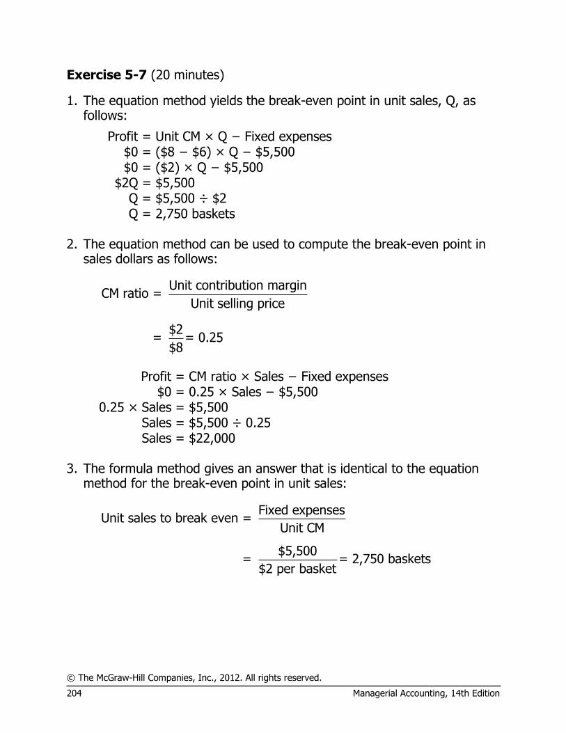
© The McGraw-Hill Companies, Inc., 2012. All rights reserved.
204 Managerial Accounting, 14th Edition
Exercise 5-7 (20 minutes)
1. The equation method yields the break-even point in unit sales, Q, as follows:
Profit = Unit CM × Q − Fixed expenses $0 = ($8 − $6) × Q − $5,500 $0 = ($2) × Q − $5,500 $2Q = $5,500 Q = $5,500 ÷ $2 Q = 2,750 baskets
2. The equation method can be used to compute the break-even point in
sales dollars as follows:
Unit contribution marginCM ratio =
Unit selling price
$2= = 0.25
$8
Profit = CM ratio × Sales − Fixed expenses $0 = 0.25 × Sales − $5,500 0.25 × Sales = $5,500 Sales = $5,500 ÷ 0.25 Sales = $22,000
3. The formula method gives an answer that is identical to the equation
method for the break-even point in unit sales:
Fixed expensesUnit sales to break even =
Unit CM
$5,500= = 2,750 baskets
$2 per basket

© The McGraw-Hill Companies, Inc., 2012. All rights reserved.
Solutions Manual, Chapter 5 205
Exercise 5-7 (continued)
4. The formula method also gives an answer that is identical to the equation method for the break-even point in dollar sales:
Fixed expensesDollar sales to break even =
CM ratio
$5,500= = $22,000
0.25
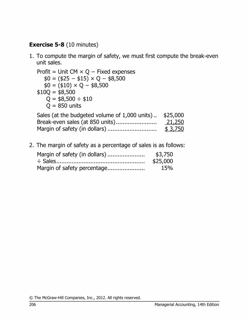
© The McGraw-Hill Companies, Inc., 2012. All rights reserved.
206 Managerial Accounting, 14th Edition
Exercise 5-8 (10 minutes)
1. To compute the margin of safety, we must first compute the break-even unit sales.
Profit = Unit CM × Q − Fixed expenses $0 = ($25 − $15) × Q − $8,500 $0 = ($10) × Q − $8,500 $10Q = $8,500 Q = $8,500 ÷ $10 Q = 850 units
Sales (at the budgeted volume of 1,000 units) .. $25,000 Break-even sales (at 850 units) ........................ 21,250 Margin of safety (in dollars) ............................. $ 3,750
2. The margin of safety as a percentage of sales is as follows:
Margin of safety (in dollars) ...................... $3,750 ÷ Sales .................................................... $25,000 Margin of safety percentage ...................... 15%
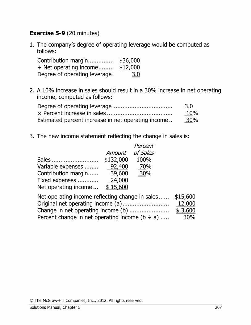
© The McGraw-Hill Companies, Inc., 2012. All rights reserved.
Solutions Manual, Chapter 5 207
Exercise 5-9 (20 minutes)
1. The company’s degree of operating leverage would be computed as follows:
Contribution margin ............... $36,000 ÷ Net operating income ......... $12,000 Degree of operating leverage . 3.0
2. A 10% increase in sales should result in a 30% increase in net operating
income, computed as follows:
Degree of operating leverage ................................... 3.0 × Percent increase in sales ...................................... 10% Estimated percent increase in net operating income .. 30%
3. The new income statement reflecting the change in sales is:
Amount Percent of Sales
Sales ........................... $132,000 100% Variable expenses ........ 92,400 70% Contribution margin ...... 39,600 30% Fixed expenses ............ 24,000 Net operating income ... $ 15,600
Net operating income reflecting change in sales ...... $15,600 Original net operating income (a) ........................... 12,000 Change in net operating income (b) ....................... $ 3,600 Percent change in net operating income (b ÷ a) ..... 30%
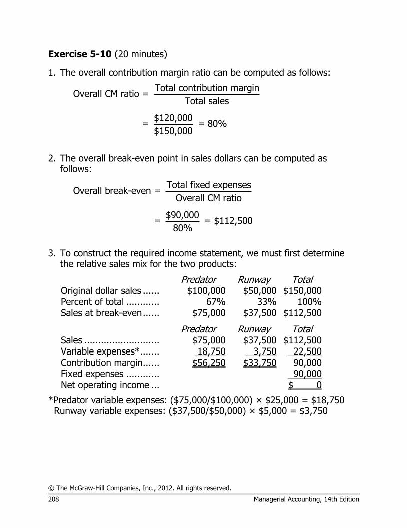
© The McGraw-Hill Companies, Inc., 2012. All rights reserved.
208 Managerial Accounting, 14th Edition
Exercise 5-10 (20 minutes)
1. The overall contribution margin ratio can be computed as follows:
Total contribution marginOverall CM ratio =
Total sales
$120,000= = 80%
$150,000
2. The overall break-even point in sales dollars can be computed as
follows:
Total fixed expensesOverall break-even =
Overall CM ratio
$90,000 = = $112,500
80%
3. To construct the required income statement, we must first determine
the relative sales mix for the two products:
Predator Runway Total Original dollar sales ...... $100,000 $50,000 $150,000 Percent of total ............ 67% 33% 100% Sales at break-even ...... $75,000 $37,500 $112,500
Predator Runway Total Sales ........................... $75,000 $37,500 $112,500 Variable expenses* ....... 18,750 3,750 22,500 Contribution margin ...... $56,250 $33,750 90,000 Fixed expenses ............ 90,000 Net operating income ... $ 0
*Predator variable expenses: ($75,000/$100,000) × $25,000 = $18,750 Runway variable expenses: ($37,500/$50,000) × $5,000 = $3,750
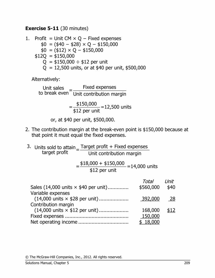
© The McGraw-Hill Companies, Inc., 2012. All rights reserved.
Solutions Manual, Chapter 5 209
Exercise 5-11 (30 minutes)
1. Profit = Unit CM × Q − Fixed expenses $0 = ($40 − $28) × Q − $150,000 $0 = ($12) × Q − $150,000 $12Q = $150,000 Q = $150,000 ÷ $12 per unit Q = 12,500 units, or at $40 per unit, $500,000 Alternatively:
Fixed expensesUnit sales =to break even Unit contribution margin
$150,000= =12,500 units
$12 per unit
or, at $40 per unit, $500,000.
2. The contribution margin at the break-even point is $150,000 because at that point it must equal the fixed expenses.
3. Target profit + Fixed expenses Units sold to attain =
target profit Unit contribution margin
$18,000 + $150,000= =14,000 units
$12 per unit
Total Unit Sales (14,000 units × $40 per unit) .............. $560,000 $40 Variable expenses
(14,000 units × $28 per unit) .................... 392,000 28 Contribution margin
(14,000 units × $12 per unit) .................... 168,000 $12 Fixed expenses ........................................... 150,000 Net operating income .................................. $ 18,000
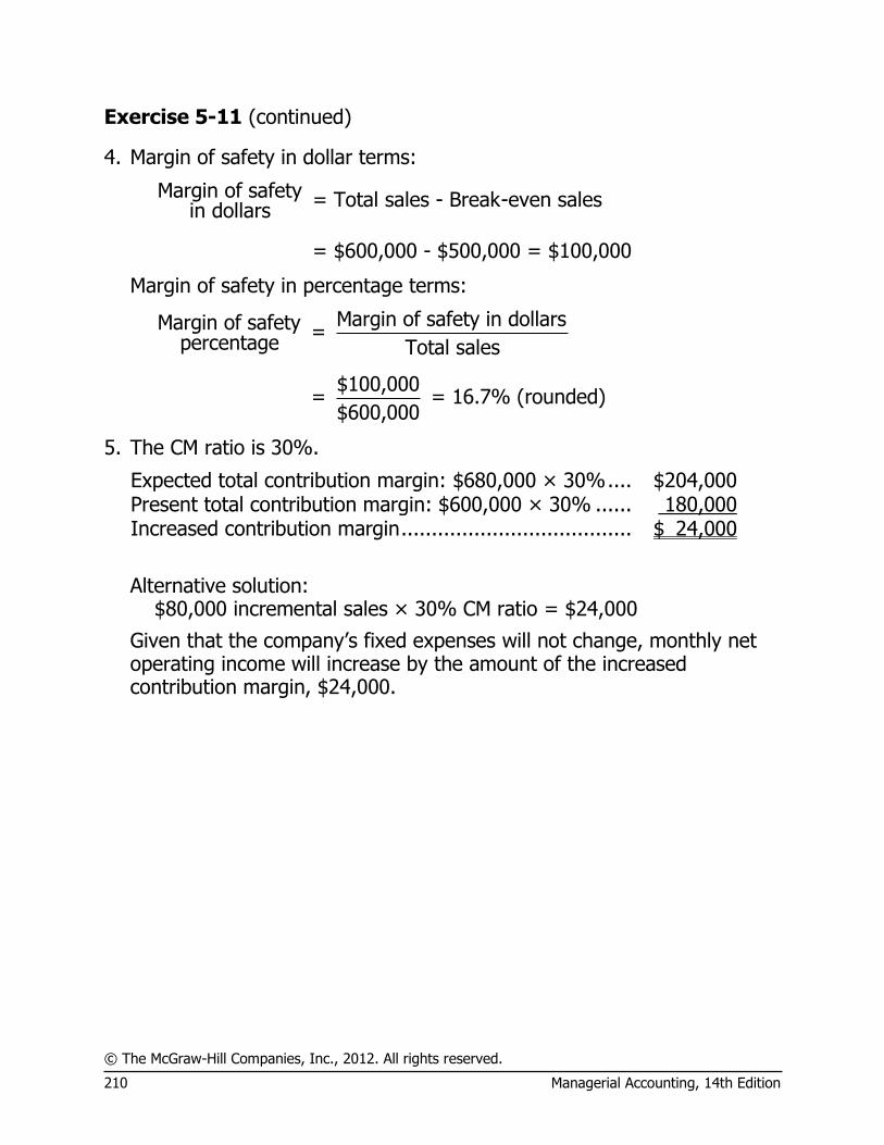
© The McGraw-Hill Companies, Inc., 2012. All rights reserved.
210 Managerial Accounting, 14th Edition
Exercise 5-11 (continued)
4. Margin of safety in dollar terms:
Margin of safety = Total sales - Break-even sales in dollars
= $600,000 - $500,000 = $100,000
Margin of safety in percentage terms:
Margin of safety in dollarsMargin of safety = percentage Total sales
$100,000= = 16.7% (rounded)
$600,000
5. The CM ratio is 30%.
Expected total contribution margin: $680,000 × 30% .... $204,000 Present total contribution margin: $600,000 × 30% ...... 180,000 Increased contribution margin ...................................... $ 24,000
Alternative solution: $80,000 incremental sales × 30% CM ratio = $24,000
Given that the company’s fixed expenses will not change, monthly net operating income will increase by the amount of the increased contribution margin, $24,000.
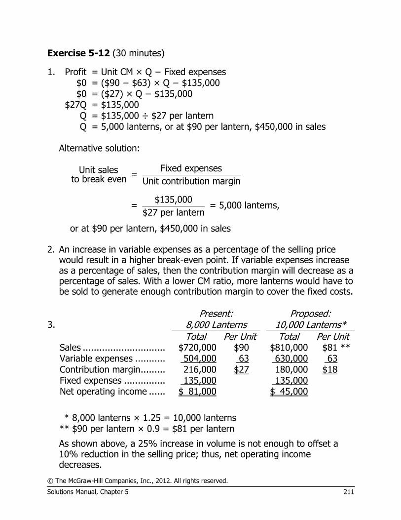
© The McGraw-Hill Companies, Inc., 2012. All rights reserved.
Solutions Manual, Chapter 5 211
Exercise 5-12 (30 minutes)
1. Profit = Unit CM × Q − Fixed expenses $0 = ($90 − $63) × Q − $135,000 $0 = ($27) × Q − $135,000 $27Q = $135,000 Q = $135,000 ÷ $27 per lantern Q = 5,000 lanterns, or at $90 per lantern, $450,000 in sales Alternative solution:
Fixed expensesUnit sales = to break even Unit contribution margin
$135,000= = 5,000 lanterns,
$27 per lantern
or at $90 per lantern, $450,000 in sales 2. An increase in variable expenses as a percentage of the selling price
would result in a higher break-even point. If variable expenses increase as a percentage of sales, then the contribution margin will decrease as a percentage of sales. With a lower CM ratio, more lanterns would have to be sold to generate enough contribution margin to cover the fixed costs.
3. Present:
8,000 Lanterns Proposed:
10,000 Lanterns* Total Per Unit Total Per Unit Sales .............................. $720,000 $90 $810,000 $81 ** Variable expenses ........... 504,000 63 630,000 63 Contribution margin ......... 216,000 $27 180,000 $18 Fixed expenses ............... 135,000 135,000 Net operating income ...... $ 81,000 $ 45,000
* 8,000 lanterns × 1.25 = 10,000 lanterns
** $90 per lantern × 0.9 = $81 per lantern
As shown above, a 25% increase in volume is not enough to offset a 10% reduction in the selling price; thus, net operating income decreases.
© The McGraw-Hill Companies, Inc., 2012. All rights reserved.
212 Managerial Accounting, 14th Edition
Exercise 5-12 (continued)
4. Profit = Unit CM × Q − Fixed expenses $72,000 = ($81 − $63) × Q − $135,000 $72,000 = ($18) × Q − $135,000 $18Q = $207,000 Q = $207,000 ÷ $18 per lantern Q = 11,500 lanterns Alternative solution:
Target profit + Fixed expenses Unit sales to attain = target profit Unit contribution margin
$72,000 + $135,000= = 11,500 lanterns
$18 per lantern

© The McGraw-Hill Companies, Inc., 2012. All rights reserved.
Solutions Manual, Chapter 5 213
Exercise 5-13 (30 minutes)
1. The contribution margin per person would be:
Price per ticket .................................................. $30 Variable expenses:
Dinner ............................................................ $7 Favors and program ........................................ 3 10
Contribution margin per person .......................... $20
The fixed expenses of the Extravaganza total $8,000; therefore, the break-even point would be computed as follows:
Profit = Unit CM × Q − Fixed expenses $0 = ($30 − $10) × Q − $8,000 $0 = ($20) × Q − $8,000 $20Q = $8,000 Q = $8,000 ÷ $20 Q = 400 persons; or, at $30 per person, $12,000 Alternative solution:
Fixed expensesUnit sales = to break even Unit contribution margin
$8,000
= = 400 persons$20 per person
or, at $30 per person, $12,000. 2. Variable cost per person ($7 + $3) ....................... $10 Fixed cost per person ($8,000 ÷ 250 persons) ...... 32 Ticket price per person to break even ................... $42
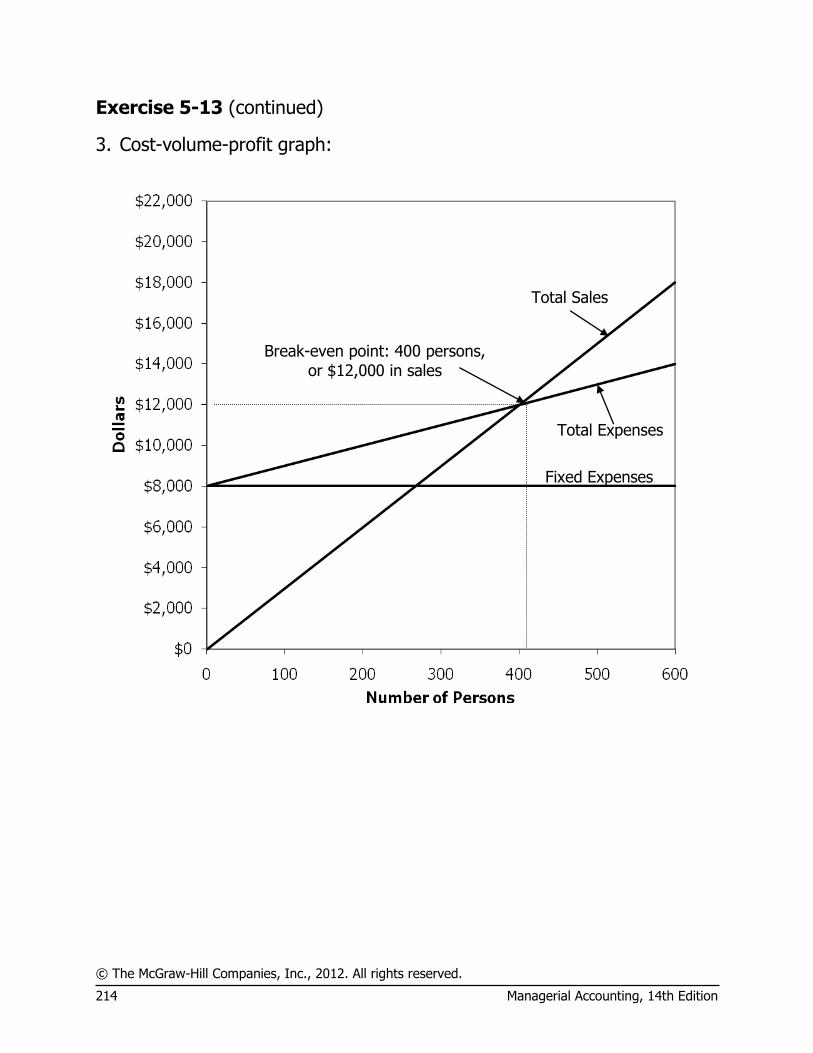
© The McGraw-Hill Companies, Inc., 2012. All rights reserved.
214 Managerial Accounting, 14th Edition
Exercise 5-13 (continued)
3. Cost-volume-profit graph:
Fixed Expenses
Total Expenses
Total Sales
Break-even point: 400 persons,
or $12,000 in sales
© The McGraw-Hill Companies, Inc., 2012. All rights reserved.
Solutions Manual, Chapter 5 215
Exercise 5-14 (30 minutes)
1. Model A100 Model B900 Total Company Amount % Amount % Amount % Sales ............... $700,000 100 $300,000 100 $1,000,000 100
Variable
expenses ....... 280,000 40 90,000 30 370,000 37
Contribution
margin .......... $420,000 60 $210,000 70 630,000 63 * Fixed expenses 598,500
Net operating
income .......... $ 31,500
*630,000 ÷ $1,000,000 = 63%. 2. The break-even point for the company as a whole is:
Fixed expensesBreak-even point in = total dollar sales Overall CM ratio
$598,500= = $950,000 in sales
0.63
3. The additional contribution margin from the additional sales is computed
as follows:
$50,000 × 63% CM ratio = $31,500
Assuming no change in fixed expenses, all of this additional contribution margin should drop to the bottom line as increased net operating income.
This answer assumes no change in selling prices, variable costs per unit, fixed expenses, or sales mix.
© The McGraw-Hill Companies, Inc., 2012. All rights reserved.
216 Managerial Accounting, 14th Edition
Exercise 5-15 (15 minutes)
1. Sales (30,000 doors) ........... $1,800,000 $60 Variable expenses ............... 1,260,000 42 Contribution margin ............. 540,000 $18 Fixed expenses ................... 450,000 Net operating income .......... $ 90,000
Contribution marginDegree of operating = leverage Net operating income
$540,000= =6
$90,000
2. a. Sales of 37,500 doors represent an increase of 7,500 doors, or 25%, over present sales of 30,000 doors. Because the degree of operating leverage is 6, net operating income should increase by 6 times as much, or by 150% (6 × 25%).
b. Expected total dollar net operating income for the next year is:
Present net operating income ............................. $ 90,000 Expected increase in net operating income next
year (150% × $90,000) .................................. 135,000 Total expected net operating income .................. $225,000
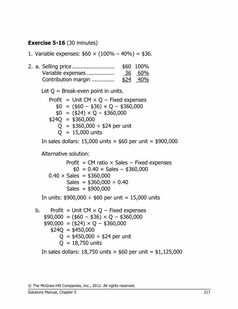
© The McGraw-Hill Companies, Inc., 2012. All rights reserved.
Solutions Manual, Chapter 5 217
Exercise 5-16 (30 minutes)
1. Variable expenses: $60 × (100% – 40%) = $36. 2. a. Selling price .......................... $60 100% Variable expenses ................. 36 60% Contribution margin .............. $24 40%
Let Q = Break-even point in units.
Profit = Unit CM × Q − Fixed expenses $0 = ($60 − $36) × Q − $360,000 $0 = ($24) × Q − $360,000
$24Q = $360,000 Q = $360,000 ÷ $24 per unit Q = 15,000 units
In sales dollars: 15,000 units × $60 per unit = $900,000 Alternative solution:
Profit = CM ratio × Sales − Fixed expenses $0 = 0.40 × Sales − $360,000
0.40 × Sales = $360,000 Sales = $360,000 ÷ 0.40 Sales = $900,000
In units: $900,000 ÷ $60 per unit = 15,000 units b. Profit = Unit CM × Q − Fixed expenses $90,000 = ($60 − $36) × Q − $360,000 $90,000 = ($24) × Q − $360,000 $24Q = $450,000 Q = $450,000 ÷ $24 per unit Q = 18,750 units
In sales dollars: 18,750 units × $60 per unit = $1,125,000

© The McGraw-Hill Companies, Inc., 2012. All rights reserved.
218 Managerial Accounting, 14th Edition
Exercise 5-16 (continued)
Alternative solution:
Profit = CM ratio × Sales − Fixed expenses $90,000 = 0.40 × Sales − $360,000
0.40 × Sales = $450,000 Sales = $450,000 ÷ 0.40 Sales = $1,125,000
In units: $1,125,000 ÷ $60 per unit = 18,750 units c. The company’s new cost/revenue relationships will be:
Selling price ...................................... $60 100% Variable expenses ($36 – $3) ............. 33 55% Contribution margin ........................... $27 45%
Profit = Unit CM × Q − Fixed expenses $0 = ($60 − $33) × Q − $360,000 $0 = $27Q − $360,000
$27Q = $360,000 Q = $360,000 ÷ $27 per unit Q = 13,333 units (rounded).
In sales dollars: 13,333 units × $60 per unit = $800,000 (rounded) Alternative solution:
Profit = CM ratio × Sales − Fixed expenses $0 = 0.45 × Sales − $360,000
0.45 × Sales = $360,000 Sales = $360,000 ÷ 0.45 Sales = $800,000
In units: $800,000 ÷ $60 per unit = 13,333 units (rounded)

© The McGraw-Hill Companies, Inc., 2012. All rights reserved.
Solutions Manual, Chapter 5 219
Exercise 5-16 (continued)
3. a. Fixed expensesUnit sales = to break even Unit contribution margin
= $360,000 ÷ $24 per unit = 15,000 units
In sales dollars: 15,000 units × $60 per unit = $900,000 Alternative solution:
Fixed expensesDollar sales = to break even CM ratio
= $360,000 ÷ 0.40 = $900,000
In units: $900,000 ÷ $60 per unit = 15,000 units
b. Target profit + Fixed expensesUnit sales to attain= target profit Unit contribution margin
= ($90,000 + $360,000) ÷ $24 per unit
= 18,750 units
In sales dollars: 18,750 units × $60 per unit = $1,125,000 Alternative solution:
Target profit + Fixed expensesDollar sales to attain= target profit CM ratio
= ($90,000 + $360,000) ÷ 0.40
= $1,125,000
In units: $1,125,000 ÷ $60 per unit = 18,750 units

© The McGraw-Hill Companies, Inc., 2012. All rights reserved.
220 Managerial Accounting, 14th Edition
Exercise 5-16 (continued)
c. Fixed expensesUnit sales =to break even Unit contribution margin
= $360,000 ÷ $27 per unit
= 13,333 units (rounded)
In sales dollars: 13,333 units × $60 per unit = $800,000 (rounded) Alternative solution:
Fixed expensesBreak-even point = in sales dollars CM ratio
= $360,000 ÷ 0.45 = $800,000
In units: $800,000 ÷ $60 per unit = 13,333 (rounded)

© The McGraw-Hill Companies, Inc., 2012. All rights reserved.
Solutions Manual, Chapter 5 221
Exercise 5-17 (20 minutes)
Total Per Unit 1. Sales (30,000 units × 1.15 = 34,500 units) .. $172,500 $5.00 Variable expenses ...................................... 103,500 3.00 Contribution margin .................................... 69,000 $2.00 Fixed expenses .......................................... 50,000 Net operating income ................................. $ 19,000 2. Sales (30,000 units × 1.20 = 36,000 units) .. $162,000 $4.50 Variable expenses ...................................... 108,000 3.00 Contribution margin .................................... 54,000 $1.50 Fixed expenses .......................................... 50,000 Net operating income ................................. $ 4,000 3. Sales (30,000 units × 0.95 = 28,500 units) .. $156,750 $5.50 Variable expenses ...................................... 85,500 3.00 Contribution margin .................................... 71,250 $2.50 Fixed expenses ($50,000 + $10,000) .......... 60,000 Net operating income ................................. $ 11,250 4. Sales (30,000 units × 0.90 = 27,000 units) .. $151,200 $5.60 Variable expenses ...................................... 86,400 3.20 Contribution margin .................................... 64,800 $2.40 Fixed expenses .......................................... 50,000 Net operating income ................................. $ 14,800
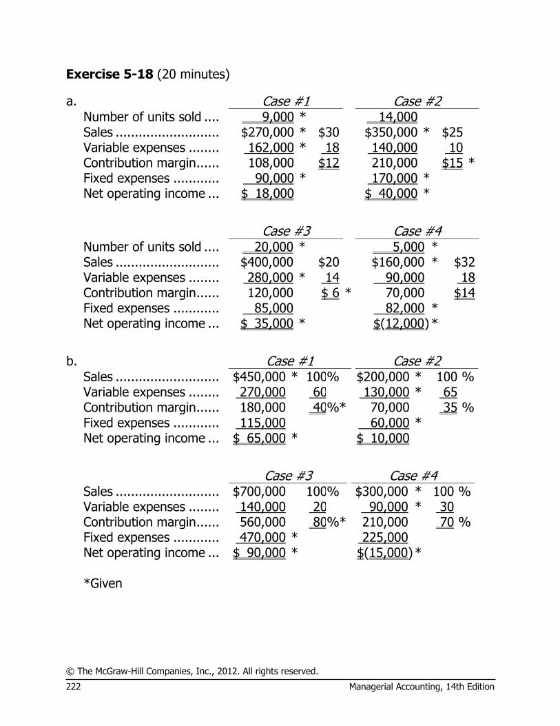
© The McGraw-Hill Companies, Inc., 2012. All rights reserved.
222 Managerial Accounting, 14th Edition
Exercise 5-18 (20 minutes)
a. Case #1 Case #2 Number of units sold .... 9,000 * 14,000 Sales ........................... $270,000 * $30 $350,000 * $25 Variable expenses ........ 162,000 * 18 140,000 10 Contribution margin ...... 108,000 $12 210,000 $15 * Fixed expenses ............ 90,000 * 170,000 * Net operating income ... $ 18,000 $ 40,000 *
Case #3 Case #4 Number of units sold .... 20,000 * 5,000 * Sales ........................... $400,000 $20 $160,000 * $32 Variable expenses ........ 280,000 * 14 90,000 18 Contribution margin ...... 120,000 $ 6 * 70,000 $14 Fixed expenses ............ 85,000 82,000 * Net operating income ... $ 35,000 * $(12,000) *
b. Case #1 Case #2 Sales ........................... $450,000 * 100 % $200,000 * 100 % Variable expenses ........ 270,000 60 130,000 * 65 Contribution margin ...... 180,000 40 %* 70,000 35 % Fixed expenses ............ 115,000 60,000 * Net operating income ... $ 65,000 * $ 10,000
Case #3 Case #4 Sales ........................... $700,000 100 % $300,000 * 100 % Variable expenses ........ 140,000 20 90,000 * 30 Contribution margin ...... 560,000 80 %* 210,000 70 % Fixed expenses ............ 470,000 * 225,000 Net operating income ... $ 90,000 * $(15,000) * *Given

© The McGraw-Hill Companies, Inc., 2012. All rights reserved.
Solutions Manual, Chapter 5 223
Problem 5-19 (60 minutes)
1. Profit = Unit CM × Q − Fixed expenses $0 = ($40 − $25) × Q − $300,000 $0 = ($15) × Q − $300,000 $15Q = $300,000 Q = $300,000 ÷ $15 per shirt Q = 20,000 shirts
20,000 shirts × $40 per shirt = $800,000 Alternative solution:
Fixed expensesUnit sales = to break even Unit contribution margin
$300,000= = 20,000 shirts
$15 per shirt
Fixed expensesDollar sales = to break even CM ratio
$300,000= = $800,000 in sales
0.375
2. See the graph on the following page. 3. The simplest approach is:
Break-even sales ................. 20,000 shirts Actual sales ......................... 19,000 shirts Sales short of break-even .... 1,000 shirts
1,000 shirts × $15 contribution margin per shirt = $15,000 loss Alternative solution:
Sales (19,000 shirts × $40 per shirt) ......................... $760,000 Variable expenses (19,000 shirts × $25 per shirt) ....... 475,000 Contribution margin .................................................. 285,000 Fixed expenses ......................................................... 300,000

© The McGraw-Hill Companies, Inc., 2012. All rights reserved.
224 Managerial Accounting, 14th Edition
Net operating loss .................................................... $(15,000)

© The McGraw-Hill Companies, Inc., 2012. All rights reserved.
Solutions Manual, Chapter 5 225
Problem 5-19 (continued)
2. Cost-volume-profit graph:
Break-even point: 20,000 shirts, or $800,000 in sales
Fixed Expenses
Total Expenses
Total Sales

© The McGraw-Hill Companies, Inc., 2012. All rights reserved.
226 Managerial Accounting, 14th Edition
Problem 5-19 (continued)
4. The variable expenses will now be $28 ($25 + $3) per shirt, and the contribution margin will be $12 ($40 – $28) per shirt.
Profit = Unit CM × Q − Fixed expenses
$0 = ($40 − $28) × Q − $300,000 $0 = ($12) × Q − $300,000
$12Q = $300,000 Q = $300,000 ÷ $12 per shirt Q = 25,000 shirts
25,000 shirts × $40 per shirt = $1,000,000 in sales Alternative solution:
Fixed expensesUnit sales = to break even Unit contribution margin
$300,000= = 25,000 shirts
$12 per shirt
Fixed expensesDollar sales = to break even CM ratio
$300,000= = $1,000,000 in sales
0.30
5. The simplest approach is:
Actual sales .................................. 23,500 shirts Break-even sales .......................... 20,000 shirts Excess over break-even sales ........ 3,500 shirts
3,500 shirts × $12 per shirt* = $42,000 profit
*$15 present contribution margin – $3 commission = $12 per shirt
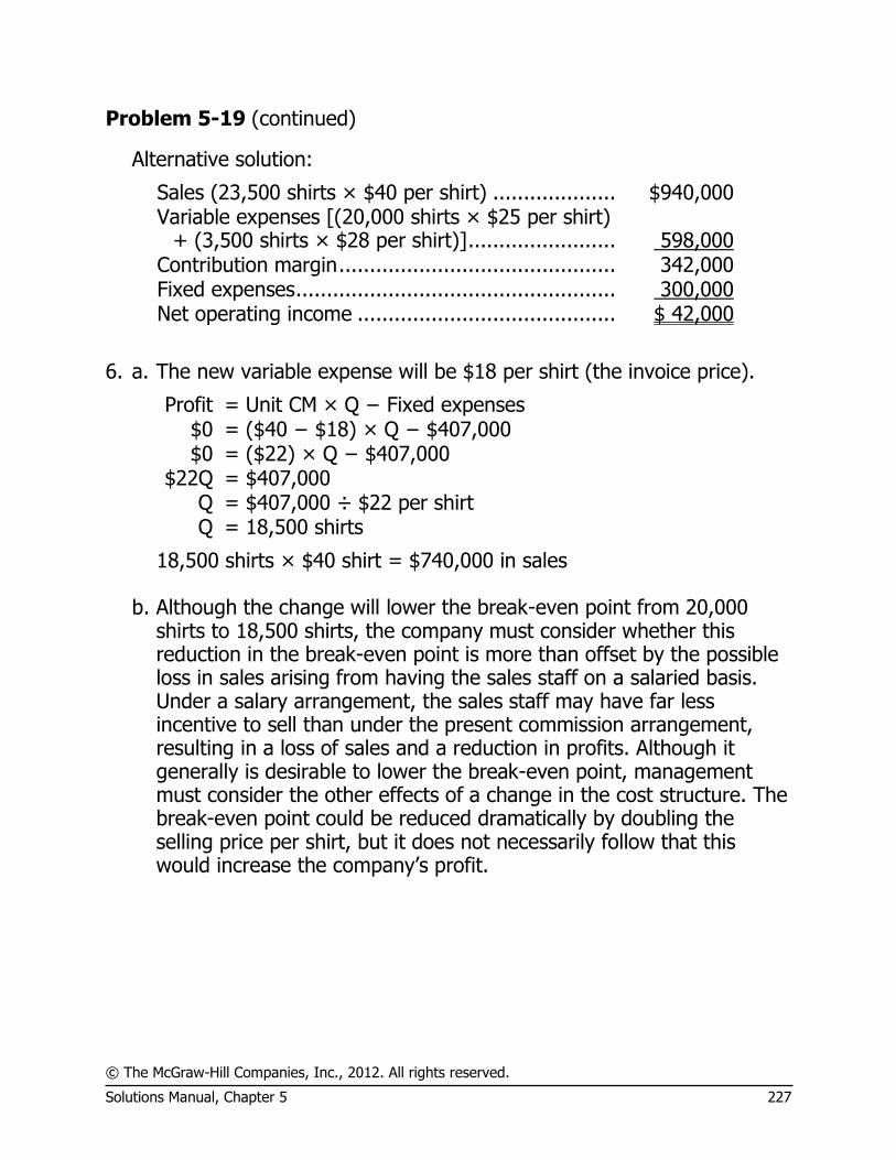
© The McGraw-Hill Companies, Inc., 2012. All rights reserved.
Solutions Manual, Chapter 5 227
Problem 5-19 (continued)
Alternative solution:
Sales (23,500 shirts × $40 per shirt) .................... $940,000 Variable expenses [(20,000 shirts × $25 per shirt)
+ (3,500 shirts × $28 per shirt)] ........................ 598,000 Contribution margin ............................................. 342,000 Fixed expenses .................................................... 300,000 Net operating income .......................................... $ 42,000
6. a. The new variable expense will be $18 per shirt (the invoice price).
Profit = Unit CM × Q − Fixed expenses $0 = ($40 − $18) × Q − $407,000 $0 = ($22) × Q − $407,000
$22Q = $407,000 Q = $407,000 ÷ $22 per shirt Q = 18,500 shirts
18,500 shirts × $40 shirt = $740,000 in sales b. Although the change will lower the break-even point from 20,000
shirts to 18,500 shirts, the company must consider whether this reduction in the break-even point is more than offset by the possible loss in sales arising from having the sales staff on a salaried basis. Under a salary arrangement, the sales staff may have far less incentive to sell than under the present commission arrangement, resulting in a loss of sales and a reduction in profits. Although it generally is desirable to lower the break-even point, management must consider the other effects of a change in the cost structure. The break-even point could be reduced dramatically by doubling the selling price per shirt, but it does not necessarily follow that this would increase the company’s profit.

© The McGraw-Hill Companies, Inc., 2012. All rights reserved.
228 Managerial Accounting, 14th Edition
Problem 5-20 (60 minutes)
1. The CM ratio is 30%.
Total Per Unit Percentage Sales (13,500 units) ......... $270,000 $20 100% Variable expenses ............ 189,000 14 70% Contribution margin ......... $ 81,000 $ 6 30%
The break-even point is:
Profit = Unit CM × Q − Fixed expenses $0 = ($20 − $14) × Q − $90,000 $0 = ($6) × Q − $90,000
$6Q = $90,000 Q = $90,000 ÷ $6 per unit Q = 15,000 units
15,000 units × $20 per unit = $300,000 in sales Alternative solution:
Fixed expensesUnit sales = to break even Unit contribution margin
$90,000= = 15,000 units
$6 per unit
Fixed expensesDollar sales = to break even CM ratio
$90,000= = $300,000 in sales
0.30
2. Incremental contribution margin: $70,000 increased sales × 30% CM ratio ........... $21,000 Less increased fixed costs: Increased advertising cost ................................. 8,000 Increase in monthly net operating income ............ $13,000
Since the company presently has a loss of $9,000 per month, if the changes are adopted, the loss will turn into a profit of $4,000 per
© The McGraw-Hill Companies, Inc., 2012. All rights reserved.
Solutions Manual, Chapter 5 229
month.

© The McGraw-Hill Companies, Inc., 2012. All rights reserved.
230 Managerial Accounting, 14th Edition
Problem 5-20 (continued)
3. Sales (27,000 units × $18 per unit*) .............. $486,000
Variable expenses
(27,000 units × $14 per unit) ...................... 378,000 Contribution margin ....................................... 108,000 Fixed expenses ($90,000 + $35,000) ............. 125,000 Net operating loss ......................................... $(17,000)
*$20 – ($20 × 0.10) = $18 4. Profit = Unit CM × Q − Fixed expenses $4,500 = ($20.00 − $14.60*) × Q − $90,000 $4,500 = ($5.40) × Q − $90,000 $5.40Q = $94,500 Q = $94,500 ÷ $5.40 per unit Q = 17,500 units *$14.00 + $0.60 = $14.60. Alternative solution:
Target profit + Fixed expensesUnit sales to attain = target profit CM per unit
$4,500 + $90,000=
$5.40 per unit**
= 17,500 units
**$6.00 – $0.60 = $5.40. 5. a. The new CM ratio would be:
Per Unit Percentage Sales ........................................... $20 100% Variable expenses ........................ 7 35% Contribution margin ..................... $13 65%

© The McGraw-Hill Companies, Inc., 2012. All rights reserved.
Solutions Manual, Chapter 5 231
Problem 5-20 (continued)
The new break-even point would be:
Fixed expensesUnit sales = to break even Unit contribution margin
$208,000= = 16,000 units
$13 per unit
Fixed expensesDollar sales = to break even CM ratio
$208,000= = $320,000 in sales
0.65
b. Comparative income statements follow:
Not Automated Automated Total Per Unit % Total Per Unit % Sales (20,000 units) .... $400,000 $20 100 $400,000 $20 100 Variable expenses ....... 280,000 14 70 140,000 7 35 Contribution margin .... 120,000 $ 6 30 260,000 $13 65 Fixed expenses ........... 90,000 208,000 Net operating income .. $ 30,000 $ 52,000

© The McGraw-Hill Companies, Inc., 2012. All rights reserved.
232 Managerial Accounting, 14th Edition
Problem 5-20 (continued)
c. Whether or not one would recommend that the company automate its operations depends on how much risk he or she is willing to take, and depends heavily on prospects for future sales. The proposed changes would increase the company’s fixed costs and its break-even point. However, the changes would also increase the company’s CM ratio (from 30% to 65%). The higher CM ratio means that once the break-even point is reached, profits will increase more rapidly than at present. If 20,000 units are sold next month, for example, the higher CM ratio will generate $22,000 more in profits than if no changes are made.
The greatest risk of automating is that future sales may drop back down to present levels (only 13,500 units per month), and as a result, losses will be even larger than at present due to the company’s greater fixed costs. (Note the problem states that sales are erratic from month to month.) In sum, the proposed changes will help the company if sales continue to trend upward in future months; the changes will hurt the company if sales drop back down to or near present levels.
Note to the Instructor: Although it is not asked for in the problem, if time permits you may want to compute the point of indifference between the two alternatives in terms of units sold; i.e., the point where profits will be the same under either alternative. At this point, total revenue will be the same; hence, we include only costs in our equation:
Let Q = Point of indifference in units sold $14Q + $90,000 = $7Q + $208,000
$7Q = $118,000 Q = $118,000 ÷ $7 per unit Q = 16,857 units (rounded)
If more than 16,857 units are sold, the proposed plan will yield the greatest profit; if less than 16,857 units are sold, the present plan will yield the greatest profit (or the least loss).

© The McGraw-Hill Companies, Inc., 2012. All rights reserved.
Solutions Manual, Chapter 5 233
Problem 5-21 (60 minutes)
1. The CM ratio is 60%:
Selling price ...................... $15 100% Variable expenses .............. 6 40% Contribution margin ........... $ 9 60%
2.
Fixed expensesBreak-even point in=total sales dollars CM ratio
$180,000= =$300,000 sales
0.60 3. $45,000 increased sales × 60% CM ratio = $27,000 increase in
contribution margin. Since fixed costs will not change, net operating income should also increase by $27,000.
4. a.
Contribution marginDegree of operating leverage =
Net operating income
$216,000= = 6
$36,000
b. 6 × 15% = 90% increase in net operating income. In dollars, this
increase would be 90% × $36,000 = $32,400.
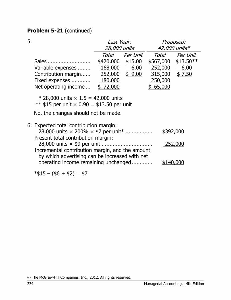
© The McGraw-Hill Companies, Inc., 2012. All rights reserved.
234 Managerial Accounting, 14th Edition
Problem 5-21 (continued)
5.
Last Year:
28,000 units Proposed:
42,000 units*
Total Per Unit Total Per Unit Sales ........................... $420,000 $15.00 $567,000 $13.50 ** Variable expenses ........ 168,000 6.00 252,000 6.00 Contribution margin ...... 252,000 $ 9.00 315,000 $ 7.50 Fixed expenses ............ 180,000 250,000 Net operating income ... $ 72,000 $ 65,000
* 28,000 units × 1.5 = 42,000 units ** $15 per unit × 0.90 = $13.50 per unit
No, the changes should not be made. 6. Expected total contribution margin:
28,000 units × 200% × $7 per unit* ................. $392,000
Present total contribution margin:
28,000 units × $9 per unit ................................ 252,000
Incremental contribution margin, and the amount by which advertising can be increased with net operating income remaining unchanged ............. $140,000
*$15 – ($6 + $2) = $7

© The McGraw-Hill Companies, Inc., 2012. All rights reserved.
Solutions Manual, Chapter 5 235
Problem 5-22 (30 minutes)
1. Product Sinks Mirrors Vanities Total
Percentage of total
sales ......................... 32% 40% 28% 100% Sales ........................... $160,000 100 % $200,000 100 % $140,000 100 % $500,000 100 % Variable expenses ........ 48,000 30 % 160,000 80 % 77,000 55 % 285,000 57 % Contribution margin ...... $112,000 70 % $ 40,000 20 % $ 63,000 45 % 215,000 43 %* Fixed expenses ............ 223,600
Net operating income
(loss) ........................ $ (8,600)
*$215,000 ÷ $500,000 = 43%.

© The McGraw-Hill Companies, Inc., 2012. All rights reserved.
236 Managerial Accounting, 14th Edition
Problem 5-22 (continued)
2. Break-even sales:
Fixed expensesDollar sales = to break even CM ratio
$223,600= = $520,000 in sales
0.43
3. Memo to the president:
Although the company met its sales budget of $500,000 for the month, the mix of products sold changed substantially from that budgeted. This is the reason the budgeted net operating income was not met, and the reason the break-even sales were greater than budgeted. The company’s sales mix was planned at 48% Sinks, 20% Mirrors, and 32% Vanities. The actual sales mix was 32% Sinks, 40% Mirrors, and 28% Vanities.
As shown by these data, sales shifted away from Sinks, which provides our greatest contribution per dollar of sales, and shifted strongly toward Mirrors, which provides our least contribution per dollar of sales. Consequently, although the company met its budgeted level of sales, these sales provided considerably less contribution margin than we had planned, with a resulting decrease in net operating income. Notice from the attached statements that the company’s overall CM ratio was only 43%, as compared to a planned CM ratio of 52%. This also explains why the break-even point was higher than planned. With less average contribution margin per dollar of sales, a greater level of sales had to be achieved to provide sufficient contribution margin to cover fixed costs.
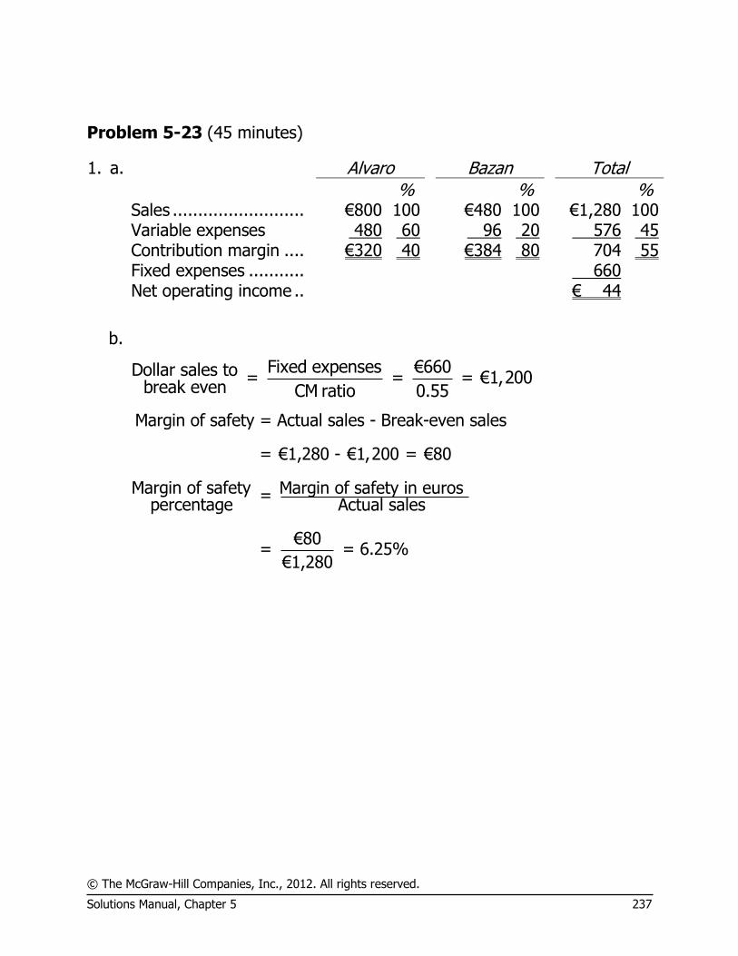
© The McGraw-Hill Companies, Inc., 2012. All rights reserved.
Solutions Manual, Chapter 5 237
Problem 5-23 (45 minutes)
1. a. Alvaro Bazan Total
% % % Sales .......................... €800 100 €480 100 €1,280 100 Variable expenses 480 60 96 20 576 45 Contribution margin .... €320 40 €384 80 704 55 Fixed expenses ........... 660 Net operating income .. € 44
b.
Fixed expenses €660Dollar sales to = = = €1,200
break even CM ratio 0.55
Margin of safety = Actual sales - Break-even sales
= €1,280 - €1,200 = €80
Margin of safety Margin of safety in euros = percentage Actual sales
€80= = 6.25%
€1,280
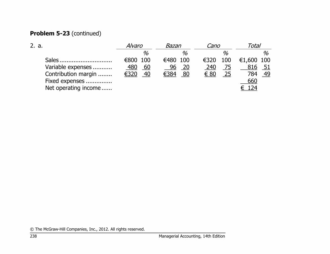
© The McGraw-Hill Companies, Inc., 2012. All rights reserved.
238 Managerial Accounting, 14th Edition
Problem 5-23 (continued)
2. a. Alvaro Bazan Cano Total % % % % Sales .............................. €800 100 €480 100 €320 100 €1,600 100 Variable expenses ........... 480 60 96 20 240 75 816 51 Contribution margin ........ €320 40 €384 80 € 80 25 784 49 Fixed expenses ............... 660 Net operating income ...... € 124

© The McGraw-Hill Companies, Inc., 2012. All rights reserved.
Solutions Manual, Chapter 5 239
Problem 5-23 (continued)
b. Fixed expenses €660Euro sales to = = = €1,347(rounded) break even CM ratio 0.49
Margin of safety = Actual sales - Break-even sales
= €1,600 - €1,347 = €253
Margin of safety Margin of safety in euros = percentage Actual sales
€253= = 15.81%
€1,600
3. The reason for the increase in the break-even point can be traced to the
decrease in the company’s average contribution margin ratio when the third product is added. Note from the income statements above that this ratio drops from 55% to 49% with the addition of the third product. This product, called Cano, has a CM ratio of only 25%, which causes the average contribution margin ratio to fall.
This problem shows the somewhat tenuous nature of break-even analysis when more than one product is involved. The manager must be very careful of his or her assumptions regarding sales mix when making decisions such as adding or deleting products.
It should be pointed out to the president that even though the break-even point is higher with the addition of the third product, the company’s margin of safety is also greater. Notice that the margin of safety increases from €80 to €253 or from 6.25% to 15.81%. Thus, the addition of the new product shifts the company much further from its break-even point, even though the break-even point is higher.

© The McGraw-Hill Companies, Inc., 2012. All rights reserved.
240 Managerial Accounting, 14th Edition
Problem 5-24 (60 minutes)
1. April's Income Statement:
Standard Deluxe Pro Total Amount % Amount % Amount % Amount % Sales ........................... $80,000 100 $60,000 100 $450,000 100 $590,000 100 Variable expenses:
Production ................. 44,000 55 27,000 45 157,500 35 228,500 38.7 Selling ....................... 4,000 5 3,000 5 22,500 5 29,500 5.0
Total variable expenses . 48,000 60 30,000 50 180,000 40 258,000 43.7 Contribution margin ...... $32,000 40 $30,000 50 $270,000 60 332,000 56.3 Fixed expenses:
Production .................. 120,000 Advertising ................. 100,000 Administrative ............. 50,000
Total fixed expenses ...... 270,000 Net operating income ..... $ 62,000

© The McGraw-Hill Companies, Inc., 2012. All rights reserved.
Solutions Manual, Chapter 5 241
Problem 5-24 (continued)
May's Income Statement:
Standard Deluxe Pro Total
Amount % Amount % Amount % Amount % Sales ............................ $320,000 100 $60,000 100 $270,000 100 $650,000 100.0 Variable expenses:
Production ................. 176,000 55 27,000 45 94,500 35 297,500 45.8 Selling ....................... 16,000 5 3,000 5 13,500 5 32,500 5.0
Total variable expenses . 192,000 60 30,000 50 108,000 40 330,000 50.8 Contribution margin ...... $128,000 40 $30,000 50 $162,000 60 320,000 49.2 Fixed expenses:
Production ................. 120,000 Advertising ................ 100,000 Administrative ............ 50,000
Total fixed expenses ..... 270,000 Net operating income .... $ 50,000

© The McGraw-Hill Companies, Inc., 2012. All rights reserved.
242 Managerial Accounting, 14th Edition
Problem 5-24 (continued)
2. The sales mix has shifted over the last month from a greater concentration of Pro rackets to a greater concentration of Standard rackets. This shift has caused a decrease in the company’s overall CM ratio from 56.3% in April to only 49.2% in May. For this reason, even though total sales (both in units and in dollars) is greater, net operating income is lower than last month in the division.
3. The break-even in dollar sales can be computed as follows:
Fixed expenses $270,000Dollar sales to = = = $479,574 (rounded) break even CM ratio 0.563
4. May’s break-even point has gone up. The reason is that the division’s overall CM ratio has declined for May as stated in (2) above. Unchanged fixed expenses divided by a lower overall CM ratio would yield a higher break-even point in sales dollars.
5. Standard Pro Increase in sales .................................. $20,000 $20,000 Multiply by the CM ratio ........................ × 40% × 60% Increase in net operating income* ......... $ 8,000 $12,000
*Assuming that fixed costs do not change.

© The McGraw-Hill Companies, Inc., 2012. All rights reserved.
Solutions Manual, Chapter 5 243
Problem 5-25 (45 minutes)
1. Sales (25,000 units × SFr 90 per unit) .................. SFr 2,250,000
Variable expenses
(25,000 units × SFr 60 per unit) ........................ 1,500,000 Contribution margin ............................................. 750,000 Fixed expenses ................................................... 840,000 Net operating loss ............................................... SFr (90,000)
2. Fixed expensesUnit sales =
to break even Unit contribution margin
SFr 840,000= = 28,000 units
SFr 30 per unit
28,000 units × SFr 90 per unit = SFr 2,520,000 to break even. 3. See the next page. 4. At a selling price of SFr 80 per unit, the contribution margin is SFr 20
per unit. Therefore:
Fixed expensesUnit sales = to break even Unit contribution margin
SFr 840,000=
SFr 20 per unit
= 42,000 units
42,000 units × SFr 80 per unit = SFr 3,360,000 to break even.
This break-even point is different from the break-even point in (2) because of the change in selling price. With the change in selling price, the unit contribution margin drops from SFr 30 to SFr 20, resulting in an increase in the break-even point.

© The McGraw-Hill Companies, Inc., 2012. All rights reserved.
244 Managerial Accounting, 14th Edition
Problem 5-25 (continued)
3. Unit SellingPrice
Unit Variable Expense
Unit Contribution
Margin Volume
Total Contribution
Margin Fixed
Expenses
Net Operating Income
(SFrs) (SFrs) (SFrs) (Units) (SFrs) (SFrs) (SFrs) 90 60 30 25,000 750,000 840,000 (90,000) 88 60 28 30,000 840,000 840,000 0 86 60 26 35,000 910,000 840,000 70,000 84 60 24 40,000 960,000 840,000 120,000 82 60 22 45,000 990,000 840,000 150,000 80 60 20 50,000 1,000,000 840,000 160,000 78 60 18 55,000 990,000 840,000 150,000 The maximum profit is SFr 160,000. This level of profit can be earned by selling 50,000 units at a
selling price of SFr 80 per unit.

© The McGraw-Hill Companies, Inc., 2012. All rights reserved.
Solutions Manual, Chapter 5 245
Problem 5-26 (60 minutes)
1. The income statements would be:
Present Amount Per Unit % Sales .............................. $800,000 $20 100% Variable expenses ............ 560,000 14 70% Contribution margin ......... 240,000 $6 30% Fixed expenses ................ 192,000 Net operating income ...... $ 48,000
Proposed
Amount Per Unit % Sales .............................. $800,000 $20 100% Variable expenses* .......... 320,000 8 40% Contribution margin ......... 480,000 $12 60% Fixed expenses ................ 432,000 Net operating income ...... $ 48,000
*$14 – $6 = $8 2. a. Degree of operating leverage:
Present:
Contribution marginDegree of = operating leverage Net operating income
$240,000= = 5
$48,000
Proposed:
Contribution marginDegree of = operating leverage Net operating income
$480,000= = 10
$48,000
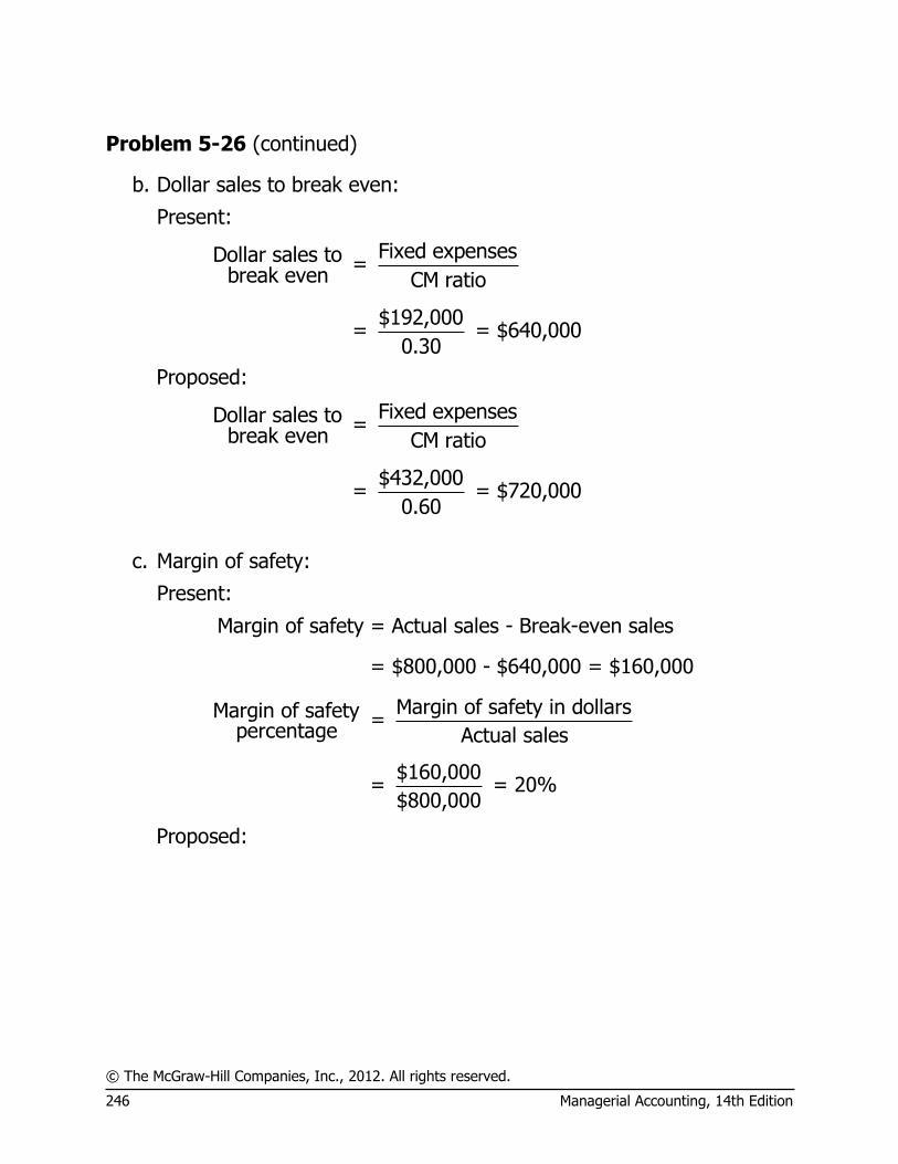
© The McGraw-Hill Companies, Inc., 2012. All rights reserved.
246 Managerial Accounting, 14th Edition
Problem 5-26 (continued)
b. Dollar sales to break even:
Present:
Fixed expensesDollar sales to = break even CM ratio
$192,000= = $640,000
0.30
Proposed:
Fixed expensesDollar sales to = break even CM ratio
$432,000= = $720,000
0.60
c. Margin of safety:
Present:
Margin of safety = Actual sales - Break-even sales
= $800,000 - $640,000 = $160,000
Margin of safety in dollarsMargin of safety = percentage Actual sales
$160,000= = 20%
$800,000
Proposed:

© The McGraw-Hill Companies, Inc., 2012. All rights reserved.
Solutions Manual, Chapter 5 247
Margin of safety = Actual sales - Break-even sales
= $800,000 - $720,000 = $80,000
Margin of safety in dollarsMargin of safety = percentage Actual sales
$80,000= = 10%
$800,000
© The McGraw-Hill Companies, Inc., 2012. All rights reserved.
248 Managerial Accounting, 14th Edition
Problem 5-26 (continued)
3. The major factor would be the sensitivity of the company’s operations to cyclical movements in the economy. Because the new equipment will increase the CM ratio, in years of strong economic activity, the company will be better off with the new equipment. However, the company will be worse off with the new equipment in years in which sales drop. The fixed costs of the new equipment will result in losses being incurred more quickly and they will be deeper. Thus, management must decide whether the potential for greater profits in good years is worth the risk of deeper losses in bad years.
4. No information is given in the problem concerning the new variable
expenses or the new contribution margin ratio. Both of these items must be determined before the new break-even point can be computed. The computations are:
New variable expenses:
Profit = (Sales − Variable expenses) − Fixed expenses $60,000** = ($1,200,000* − Variable expenses) − $240,000
Variable expenses = $1,200,000 − $240,000 − $60,000 = $900,000
* New level of sales: $800,000 × 1.5 = $1,200,000 ** New level of net operating income: $48,000 × 1.25 = $60,000
New CM ratio:
Sales .................................... $1,200,000 100% Variable expenses .................. 900,000 75% Contribution margin ............... $ 300,000 25%
With the above data, the new break-even point can be computed:
Fixed expenses $240,000Dollar sales = = =$960,000
to break even CM ratio 0.25
© The McGraw-Hill Companies, Inc., 2012. All rights reserved.
Solutions Manual, Chapter 5 249
Problem 5-26 (continued)
The greatest risk is that the increases in sales and net operating income predicted by the marketing manager will not happen and that sales will remain at their present level. Note that the present level of sales is $800,000, which is well below the break-even level of sales under the new marketing strategy.
It would be a good idea to compare the new marketing strategy to the current situation more directly. What level of sales would be needed under the new method to generate at least the $48,000 in profits the company is currently earning each month? The computations are:
Target profit + Fixed expensesDollar sales to attain= target profit CM ratio
$48,000 + $240,000=
0.25
= $1,152,000 in sales each month
Thus, sales would have to increase by at least 44% ($1,152,000 is 44% higher than $800,000) in order to make the company better off with the new marketing strategy than with the current approach. This appears to be extremely risky.
© The McGraw-Hill Companies, Inc., 2012. All rights reserved.
250 Managerial Accounting, 14th Edition
Problem 5-27 (30 minutes)
1. The numbered components are as follows:
(1) Dollars of revenue and costs. (2)
Volume of output, expressed in units, % of capacity, sales,
or some other measure of activity. (3) Total expense line. (4) Variable expense area. (5) Fixed expense area. (6) Break-even point. (7) Loss area. (8) Profit area. (9) Revenue line.
© The McGraw-Hill Companies, Inc., 2012. All rights reserved.
Solutions Manual, Chapter 5 251
Problem 5-27 (continued)
2. a. Line 3: Remain unchanged. Line 9: Have a flatter slope. Break-even point: Increase.
b. Line 3: Have a steeper slope. Line 9: Remain unchanged. Break-even point: Increase.
c. Line 3: Shift downward. Line 9: Remain unchanged. Break-even point: Decrease.
d. Line 3: Remain unchanged. Line 9: Remain unchanged. Break-even point: Remain unchanged.
e. Line 3: Shift upward and have a flatter slope. Line 9: Remain unchanged.
Break-even point:
Probably change, but the direction is
uncertain.
f. Line 3: Have a flatter slope. Line 9: Have a flatter slope.
Break-even point:
Remain unchanged in terms of units;
decrease in terms of total dollars of sales.
g. Line 3: Shift upward. Line 9: Remain unchanged. Break-even point: Increase.
h. Line 3: Shift downward and have a steeper slope. Line 9: Remain unchanged.
Break-even point:
Probably change, but the direction is
uncertain.
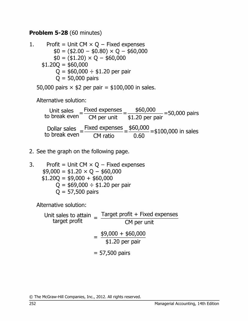
© The McGraw-Hill Companies, Inc., 2012. All rights reserved.
252 Managerial Accounting, 14th Edition
Problem 5-28 (60 minutes)
1. Profit = Unit CM × Q − Fixed expenses $0 = ($2.00 − $0.80) × Q − $60,000 $0 = ($1.20) × Q − $60,000 $1.20Q = $60,000 Q = $60,000 ÷ $1.20 per pair Q = 50,000 pairs
50,000 pairs × $2 per pair = $100,000 in sales. Alternative solution:
Fixed expenses $60,000Unit sales = = =50,000 pairs
to break even CM per unit $1.20 per pair
Fixed expenses $60,000Dollar sales = = =$100,000 in sales
to break even CM ratio 0.60
2. See the graph on the following page. 3. Profit = Unit CM × Q − Fixed expenses $9,000 = $1.20 × Q − $60,000 $1.20Q = $9,000 + $60,000 Q = $69,000 ÷ $1.20 per pair Q = 57,500 pairs Alternative solution:
Target profit + Fixed expensesUnit sales to attain = target profit CM per unit
$9,000 + $60,000=
$1.20 per pair
= 57,500 pairs

© The McGraw-Hill Companies, Inc., 2012. All rights reserved.
Solutions Manual, Chapter 5 253
Problem 5-28 (continued)
2. Cost-volume-profit graph:
Break-even point: 50,000 pairs, or $100,000 in sales
Fixed Expenses
Total Expenses
Total Sales
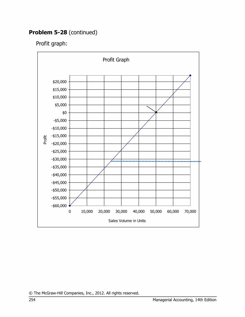
© The McGraw-Hill Companies, Inc., 2012. All rights reserved.
254 Managerial Accounting, 14th Edition
Problem 5-28 (continued)
Profit graph:
Break-even point: 50,000 pairs of
stockings
Profit Graph
-$60,000
-$55,000
-$50,000
-$45,000
-$40,000
-$35,000
-$30,000
-$25,000
-$20,000
-$15,000
-$10,000
-$5,000
$0
$5,000
$10,000
$15,000
$20,000
0 10,000 20,000 30,000 40,000 50,000 60,000 70,000
Sales Volume in Units
Pro
fit

© The McGraw-Hill Companies, Inc., 2012. All rights reserved.
Solutions Manual, Chapter 5 255
Problem 5-28 (continued)
4. Incremental contribution margin: $20,000 increased sales × 60% CM ratio ........... $12,000 Less incremental fixed salary cost ........................ 8,000 Increased net operating income ........................... $ 4,000
Yes, the position should be converted to a full-time basis. 5. a. Contribution margin $75,000Degree of = = = 5
operating leverage Net operating income $15,000
b. 5 × 20% sales increase = 100% increase in net operating income. Thus, net operating income would double next year, going from $15,000 to $30,000.
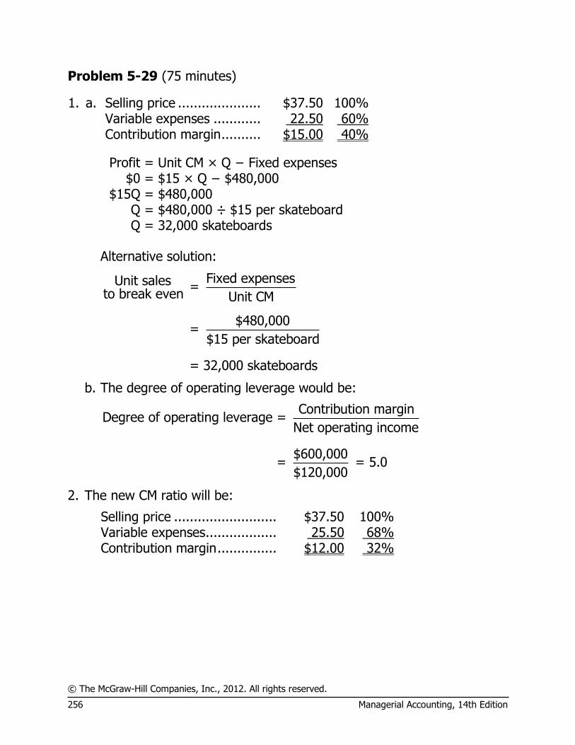
© The McGraw-Hill Companies, Inc., 2012. All rights reserved.
256 Managerial Accounting, 14th Edition
Problem 5-29 (75 minutes)
1. a. Selling price ..................... $37.50 100% Variable expenses ............ 22.50 60% Contribution margin .......... $15.00 40%
Profit = Unit CM × Q − Fixed expenses $0 = $15 × Q − $480,000 $15Q = $480,000 Q = $480,000 ÷ $15 per skateboard Q = 32,000 skateboards
Alternative solution:
Fixed expensesUnit sales = to break even Unit CM
$480,000=
$15 per skateboard
= 32,000 skateboards
b. The degree of operating leverage would be:
Contribution marginDegree of operating leverage =
Net operating income
$600,000= = 5.0
$120,000
2. The new CM ratio will be:
Selling price .......................... $37.50 100% Variable expenses .................. 25.50 68% Contribution margin ............... $12.00 32%
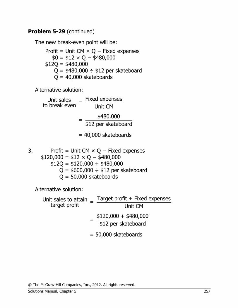
© The McGraw-Hill Companies, Inc., 2012. All rights reserved.
Solutions Manual, Chapter 5 257
Problem 5-29 (continued)
The new break-even point will be:
Profit = Unit CM × Q − Fixed expenses $0 = $12 × Q − $480,000 $12Q = $480,000 Q = $480,000 ÷ $12 per skateboard Q = 40,000 skateboards
Alternative solution:
Fixed expensesUnit sales = to break even Unit CM
$480,000=
$12 per skateboard
= 40,000 skateboards
3. Profit = Unit CM × Q − Fixed expenses $120,000 = $12 × Q − $480,000 $12Q = $120,000 + $480,000 Q = $600,000 ÷ $12 per skateboard Q = 50,000 skateboards Alternative solution:
Target profit + Fixed expensesUnit sales to attain = target profit Unit CM
$120,000 + $480,000=
$12 per skateboard
= 50,000 skateboards
© The McGraw-Hill Companies, Inc., 2012. All rights reserved.
258 Managerial Accounting, 14th Edition
Problem 5-29 (continued)
Thus, sales will have to increase by 10,000 skateboards (50,000 skateboards, less 40,000 skateboards currently being sold) to earn the same amount of net operating income as earned last year. The computations above and in part (2) show the dramatic effect that increases in variable costs can have on an organization. These effects from a $3 per unit increase in labor costs for Tyrene Company are summarized below:
Present Expected Break-even point (in skateboards) ........... 32,000 40,000 Sales (in skateboards) needed to earn net
operating income of $120,000 .............. 40,000 50,000
Note that if variable costs do increase next year, then the company will just break even if it sells the same number of skateboards (40,000) as it did last year.
4. The contribution margin ratio last year was 40%. If we let P equal the
new selling price, then:
P = $25.50 + 0.40P 0.60P = $25.50
P = $25.50 ÷ 0.60 P = $42.50
To verify: Selling price ............................ $42.50 100% Variable expenses ................... 25.50 60% Contribution margin ................ $17.00 40%
Therefore, to maintain a 40% CM ratio, a $3 increase in variable costs would require a $5 increase in the selling price.
© The McGraw-Hill Companies, Inc., 2012. All rights reserved.
Solutions Manual, Chapter 5 259
Problem 5-29 (continued)
5. The new CM ratio would be:
Selling price ........................ $37.50 100% Variable expenses ................ 13.50 * 36% Contribution margin ............. $24.00 64%
*$22.50 – ($22.50 × 40%) = $13.50
The new break-even point would be:
Profit = Unit CM × Q − Fixed expenses $0 = $24 × Q − $912,000* $24Q = $912,000 Q = $912,000 ÷ $24 per skateboard Q = 38,000 skateboards
*$480,000 × 1.9 = $912,000 Alternative solution:
Fixed expensesUnit sales = to break even Unit CM
$912,000=
$24 per skateboard
= 38,000 skateboards
Although this break-even figure is greater than the company’s present break-even figure of 32,000 skateboards [see part (1) above], it is less than the break-even point will be if the company does not automate and variable labor costs rise next year [see part (2) above].
© The McGraw-Hill Companies, Inc., 2012. All rights reserved.
260 Managerial Accounting, 14th Edition
Problem 5-29 (continued)
6. a. Profit = Unit CM × Q − Fixed expenses $120,000 = $24 × Q − $912,000* $24Q = $120,000 + $912,000 Q = $1,032,000 ÷ $24.00 per skateboard Q = 43,000 skateboards
*480,000 × 1.9 = $912,000
Alternative solution:
Target profit + Fixed expensesUnit sales to attain = target profit Unit CM
$120,000 + $912,000=
$24 per skateboard
= 43,000 skateboards
Thus, the company will have to sell 3,000 more skateboards (43,000 – 40,000 = 3,000) than now being sold to earn a profit of $120,000 each year. However, this is still less than the 50,000 skateboards that would have to be sold to earn a $120,000 profit if the plant is not automated and variable labor costs rise next year [see part (3) above].
© The McGraw-Hill Companies, Inc., 2012. All rights reserved.
Solutions Manual, Chapter 5 261
Problem 5-29 (continued)
b. The contribution income statement would be:
Sales (40,000 skateboards × $37.50 per skateboard) .. $1,500,000
Variable expenses (40,000 skateboards × $13.50 per skateboard) . 540,000
Contribution margin ............................................ 960,000 Fixed expenses ................................................... 912,000 Net operating income .......................................... $ 48,000
Contribution marginDegree of operating = leverage Net operating income
$960,000= = 20
$48,000
c. This problem shows the difficulty faced by some companies. When variable labor costs increase, it is often difficult to pass these cost increases along to customers in the form of higher prices. Thus, companies are forced to automate, resulting in higher operating leverage, often a higher break-even point, and greater risk for the company.
There is no clear answer as to whether one should have been in favor of constructing the new plant.

© The McGraw-Hill Companies, Inc., 2012. All rights reserved.
262 Managerial Accounting, 14th Edition
Problem 5-30 (30 minutes)
1. The contribution margin per stein would be:
Selling price ........................................................ $30 Variable expenses:
Purchase cost of the steins ................................ $15 Commissions to the student salespersons ........... 6 21
Contribution margin ............................................. $ 9
Since there are no fixed costs, the number of unit sales needed to yield the desired $7,200 in profits can be obtained by dividing the target profit by the unit contribution margin:
Target profit $7,200 = = 800 steins
Unit CM $9 per stein
800 steins × $30 per stein = $24,000 in total sales
2. Since an order has been placed, there is now a ―fixed‖ cost associated with the purchase price of the steins (i.e., the steins can’t be returned). For example, an order of 200 steins requires a ―fixed‖ cost (investment) of $3,000 (= 200 steins × $15 per stein). The variable costs drop to only $6 per stein, and the new contribution margin per stein becomes:
Selling price ................................................ $30 Variable expenses (commissions only) .......... 6 Contribution margin ..................................... $24
Since the ―fixed‖ cost of $3,000 must be recovered before Marbury
shows any profit, the break-even computation would be:
Fixed expenses $3,000Unit sales = = =125 steinsto break even Unit CM $24 per stein
125 steins × $30 per stein =$3,750 in total sales
If a quantity other than 200 steins were ordered, the answer would change accordingly.

© The McGraw-Hill Companies, Inc., 2012. All rights reserved.
Solutions Manual, Chapter 5 263
Problem 5-31 (45 minutes)
1. The contribution margin per unit on the first 30,000 units is:
Per Unit Selling price .......................... $2.50 Variable expenses .................. 1.60 Contribution margin ............... $0.90
The contribution margin per unit on anything over 30,000 units is:
Per Unit Selling price .......................... $2.50 Variable expenses .................. 1.75 Contribution margin ............... $0.75
Thus, for the first 30,000 units sold, the total amount of contribution margin generated would be:
30,000 units × $0.90 per unit = $27,000. Since the fixed costs on the first 30,000 units total $40,000, the $27,000
contribution margin above is not enough to permit the company to break even. Therefore, in order to break even, more than 30,000 units will have to be sold. The fixed costs that will have to be covered by the additional sales are:
Fixed costs on the first 30,000 units .......................... $40,000 Less contribution margin from the first 30,000 units ... 27,000 Remaining unrecovered fixed costs ............................ 13,000 Add monthly rental cost of the additional space
needed to produce more than 30,000 units ............. 2,000 Total fixed costs to be covered by remaining sales ...... $15,000

© The McGraw-Hill Companies, Inc., 2012. All rights reserved.
264 Managerial Accounting, 14th Edition
Problem 5-31 (continued)
The additional sales of units required to cover these fixed costs would be:
Total remaining fixed costs $15,000=
Unit contribution margin on added units $0.75 per unit
=20,000 units
Therefore, a total of 50,000 units (30,000 + 20,000) must be sold for the company to break even. This number of units would equal total sales of:
50,000 units × $2.50 per unit = $125,000 in total sales. 2. Target profit $9,000
= =12,000 unitsUnit contribution margin $0.75 per unit
Thus, the company must sell 12,000 units above the break-even point to earn a profit of $9,000 each month. These units, added to the 50,000 units required to break even, equal total sales of 62,000 units each month to reach the target profit.
3. If a bonus of $0.15 per unit is paid for each unit sold in excess of the
break-even point, then the contribution margin on these units would drop from $0.75 to only $0.60 per unit.
The desired monthly profit would be:
25% × ($40,000 + $2,000) = $10,500
Thus,
Target profit $10,500
= =17,500 unitsUnit contribution margin $0.60 per unit
Therefore, the company must sell 17,500 units above the break-even point to earn a profit of $10,500 each month. These units, added to the 50,000 units required to break even, would equal total sales of 67,500 units each month.

© The McGraw-Hill Companies, Inc., 2012. All rights reserved.
Solutions Manual, Chapter 5 265
Case 5-32 (75 minutes)
1. The contribution format income statements (in thousands of dollars) for the three alternatives are:
18% Commission 20% Commission Own Sales Force Sales ................................................. $30,000 100 % $30,000 100 % $30,000 100 % Variable expenses:
Variable cost of goods sold ............... 17,400 17,400 17,400 Commissions ................................... 5,400 6,000 3,000
Total variable expense ........................ 22,800 76 % 23,400 78 % 20,400 68 % Contribution margin ............................ 7,200 24 % 6,600 22 % 9,600 32 % Fixed expenses:
Fixed cost of goods sold ................... 2,800 2,800 2,800 Fixed advertising expense ................. 800 800 1,300 * Fixed marketing staff expense .......... 1,300 ** Fixed administrative expense ............ 3,200 3,200 3,200
Total fixed expenses ........................... 6,800 6,800 8,600 Net operating income ......................... $ 400 $ (200) $ 1,000
* $800,000 + $500,000 = $1,300,000 ** $700,000 + $400,000 + $200,000 = $1,300,000
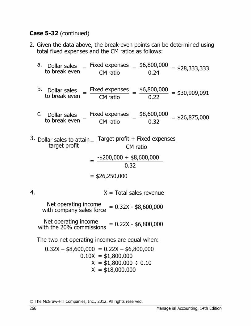
© The McGraw-Hill Companies, Inc., 2012. All rights reserved.
266 Managerial Accounting, 14th Edition
Case 5-32 (continued)
2. Given the data above, the break-even points can be determined using total fixed expenses and the CM ratios as follows:
a. Fixed expenses $6,800,000Dollar sales = = = $28,333,333
to break even CM ratio 0.24
b. Fixed expenses $6,800,000Dollar sales = = = $30,909,091
to break even CM ratio 0.22
c. Fixed expenses $8,600,000Dollar sales = = = $26,875,000
to break even CM ratio 0.32
3. Target profit + Fixed expensesDollar sales to attain=
target profit CM ratio
-$200,000 + $8,600,000=
0.32
= $26,250,000
4. X = Total sales revenue
Net operating income = 0.32X - $8,600,000with company sales force
Net operating income = 0.22X - $6,800,000with the 20% commissions
The two net operating incomes are equal when:
0.32X – $8,600,000 = 0.22X – $6,800,000 0.10X = $1,800,000
X = $1,800,000 ÷ 0.10 X = $18,000,000
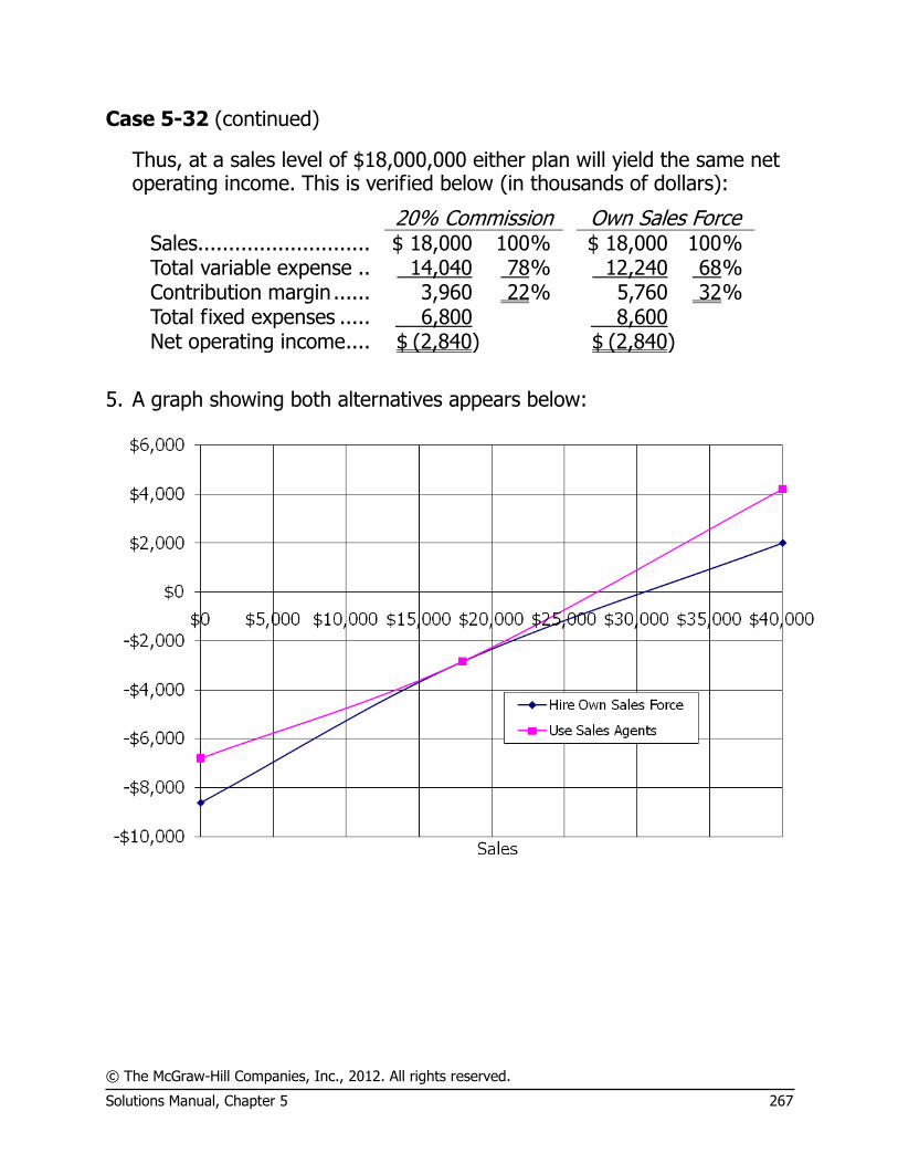
© The McGraw-Hill Companies, Inc., 2012. All rights reserved.
Solutions Manual, Chapter 5 267
Case 5-32 (continued)
Thus, at a sales level of $18,000,000 either plan will yield the same net operating income. This is verified below (in thousands of dollars):
20% Commission Own Sales Force Sales ............................ $ 18,000 100 % $ 18,000 100 % Total variable expense .. 14,040 78 % 12,240 68 % Contribution margin ...... 3,960 22 % 5,760 32 % Total fixed expenses ..... 6,800 8,600 Net operating income .... $ (2,840) $ (2,840)
5. A graph showing both alternatives appears below:

© The McGraw-Hill Companies, Inc., 2012. All rights reserved.
268 Managerial Accounting, 14th Edition
Case 5-32 (continued) 6. To: President of Marston Corporation Fm: Student’s name
Assuming that a competent sales force can be quickly hired and trained and the new sales force is as effective as the sales agents, this is the better alternative. Using the data provided by the controller, unless sales fall below $18,000,000 net operating income is higher when the company has its own sales force. At that level of sales and below, the company would be losing money, so it is unlikely that this would be the normal situation.
The major concern I have with this recommendation is the assumption that the new sales force will be as effective as the sales agents. The sales agents have been selling our product for a number of years, so they are likely to have more field experience than any sales force we hire. And, our own sales force would be selling just our product instead of a variety of products. On the one hand, that will result in a more focused selling effort. On the other hand, that may make it more difficult for a salesperson to get the attention of a hospital’s purchasing agent.
The purchasing agents may prefer to deal through a small number of salespersons, each of whom sells many products, rather than a large number of salespersons each of whom sells only a single product. Even so, we can afford some decrease in sales because of the lower cost of maintaining our own sales force. For example, assuming that the sales agents make the budgeted sales of $30,000,000, we would have a net operating loss of $200,000 for the year. We would do better than this with our own sales force as long as sales are greater than $26,250,000. In other words, we could afford a fall-off in sales of $3,750,000, or 12.5%, and still be better off with our own sales force. If we are confident that our own sales force could do at least this well relative to the sales agents, then we should certainly switch to using our own sales force.
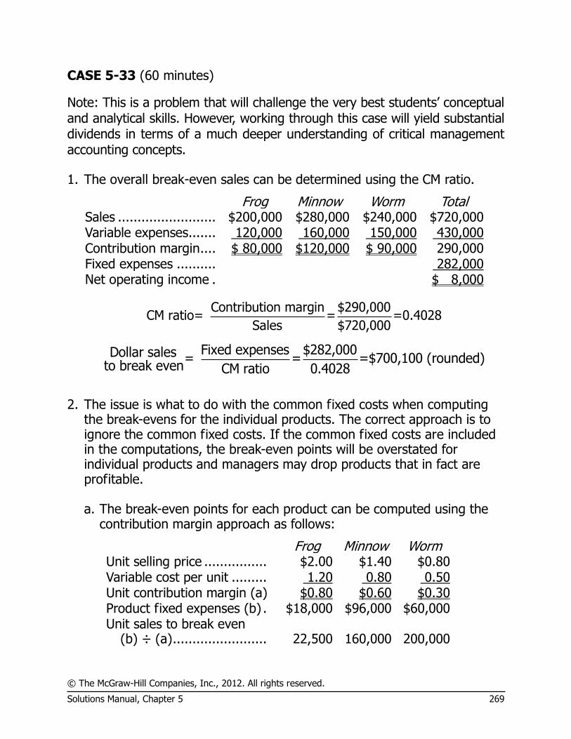
© The McGraw-Hill Companies, Inc., 2012. All rights reserved.
Solutions Manual, Chapter 5 269
CASE 5-33 (60 minutes)
Note: This is a problem that will challenge the very best students’ conceptual and analytical skills. However, working through this case will yield substantial dividends in terms of a much deeper understanding of critical management accounting concepts. 1. The overall break-even sales can be determined using the CM ratio.
Frog Minnow Worm Total Sales ......................... $200,000 $280,000 $240,000 $720,000 Variable expenses ....... 120,000 160,000 150,000 430,000 Contribution margin .... $ 80,000 $120,000 $ 90,000 290,000 Fixed expenses .......... 282,000 Net operating income . $ 8,000
Contribution margin $290,000CM ratio= = =0.4028
Sales $720,000
Fixed expenses $282,000Dollar sales = = =$700,100 (rounded)to break even CM ratio 0.4028
2. The issue is what to do with the common fixed costs when computing
the break-evens for the individual products. The correct approach is to ignore the common fixed costs. If the common fixed costs are included in the computations, the break-even points will be overstated for individual products and managers may drop products that in fact are profitable.
a. The break-even points for each product can be computed using the
contribution margin approach as follows:
Frog Minnow Worm Unit selling price ................ $2.00 $1.40 $0.80 Variable cost per unit ......... 1.20 0.80 0.50 Unit contribution margin (a) $0.80 $0.60 $0.30 Product fixed expenses (b) . $18,000 $96,000 $60,000
Unit sales to break even
(b) ÷ (a) ........................ 22,500 160,000 200,000

© The McGraw-Hill Companies, Inc., 2012. All rights reserved.
270 Managerial Accounting, 14th Edition
Case 5-33 (continued)
b. If the company were to sell exactly the break-even quantities computed above, the company would lose $108,000—the amount of the common fixed cost. This occurs because the common fixed costs have been ignored in the calculations of the break-evens.
The fact that the company loses $108,000 if it operates at the level of sales indicated by the break-evens for the individual products can be verified as follows:
Frog Minnow Worm Total Unit sales ................ 22,500 160,000 200,000 Sales ....................... $45,000 $224,000 $160,000 $ 429,000 Variable expenses .... 27,000 128,000 100,000 255,000 Contribution margin . $18,000 $ 96,000 $ 60,000 174,000 Fixed expenses ........ 282,000 Net operating loss .... $(108,000)
At this point, many students conclude that something is wrong with
their answer to part (a) because the company loses money operating at the break-evens for the individual products. They also worry that managers may be lulled into a false sense of security if they are given the break-evens computed in part (a). Total sales at the individual product break-evens is only $429,000 whereas the total sales at the overall break-even computed in part (1) is $700,100.
Many students (and managers, for that matter) attempt to resolve this apparent paradox by allocating the common fixed costs among the products prior to computing the break-evens for individual products. Any of a number of allocation bases could be used for this purpose—sales, variable expenses, product-specific fixed expenses, contribution margins, etc. (We usually take a tally of how many students allocated the common fixed costs using each possible allocation base before proceeding.) For example, the common fixed costs are allocated on the next page based on sales.
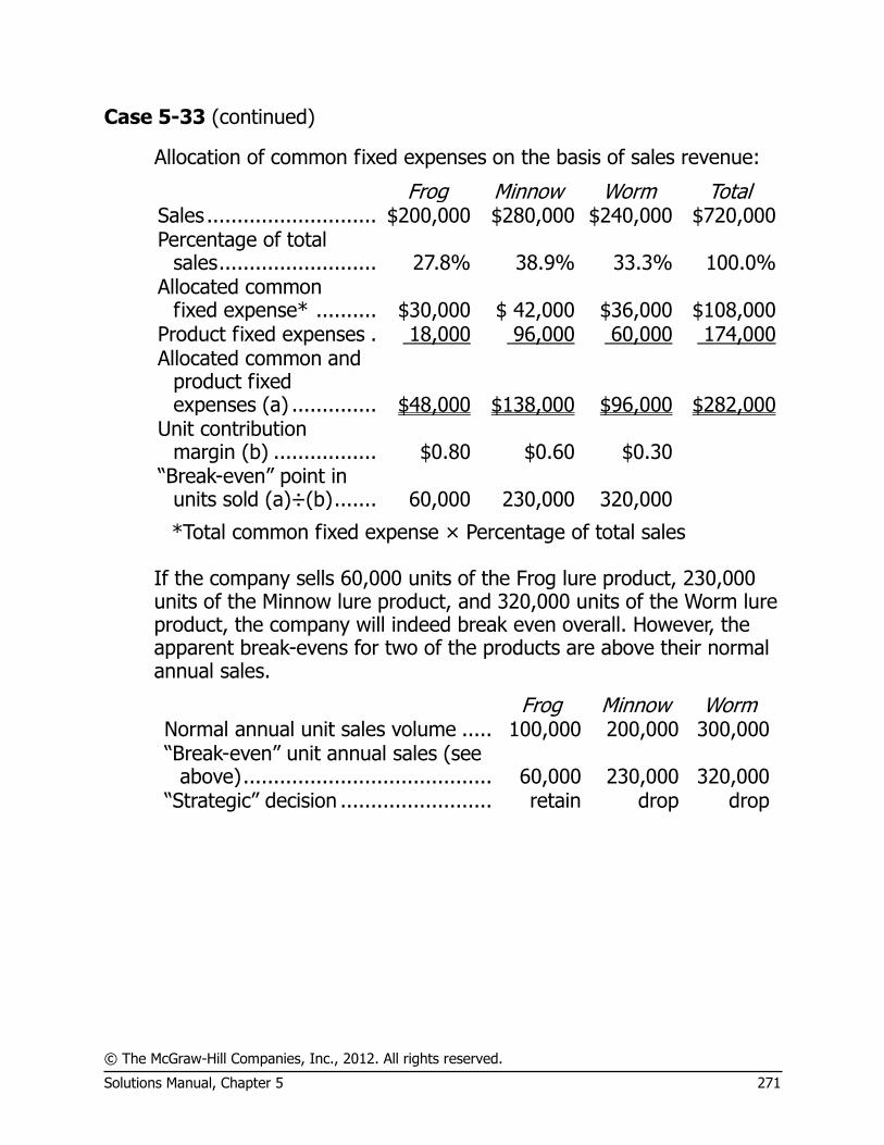
© The McGraw-Hill Companies, Inc., 2012. All rights reserved.
Solutions Manual, Chapter 5 271
Case 5-33 (continued)
Allocation of common fixed expenses on the basis of sales revenue:
Frog Minnow Worm Total Sales ............................ $200,000 $280,000 $240,000 $720,000
Percentage of total
sales .......................... 27.8% 38.9% 33.3% 100.0%
Allocated common
fixed expense* .......... $30,000 $ 42,000 $36,000 $108,000 Product fixed expenses . 18,000 96,000 60,000 174,000
Allocated common and product fixed expenses (a) .............. $48,000 $138,000 $96,000 $282,000
Unit contribution
margin (b) ................. $0.80 $0.60 $0.30
―Break-even‖ point in
units sold (a)÷(b) ....... 60,000 230,000 320,000
*Total common fixed expense × Percentage of total sales If the company sells 60,000 units of the Frog lure product, 230,000
units of the Minnow lure product, and 320,000 units of the Worm lure product, the company will indeed break even overall. However, the apparent break-evens for two of the products are above their normal annual sales.
Frog Minnow Worm Normal annual unit sales volume ..... 100,000 200,000 300,000
―Break-even‖ unit annual sales (see
above) ......................................... 60,000 230,000 320,000 ―Strategic‖ decision ......................... retain drop drop

© The McGraw-Hill Companies, Inc., 2012. All rights reserved.
272 Managerial Accounting, 14th Edition
Case 5-33 (continued)
It would be natural to interpret a break-even for a product as the level of sales below which the company would be financially better off dropping the product. Therefore, we should not be surprised if managers, based on the erroneous break-even calculation on the previous page, would decide to drop the Minnow and Worm lures and concentrate on the company’s ―core competency,‖ which appears to be the Frog lure. However, if they were to do that, the company would face a loss of $46,000:
Frog Minnow Worm Total Sales .......................... $200,000 dropped dropped $200,000 Variable expenses ....... 120,000 120,000 Contribution margin .... $ 80,000 80,000 Fixed expenses* ......... 126,000 Net operating loss ....... $(46,000)
*By dropping the two products, the company reduces its fixed expenses by only $156,000 (= $96,000 + $60,000). Therefore, the total fixed expenses would be $126,000 (= $282,000 − $156,000).
By dropping the two products, the company would have a loss of $46,000 rather than a profit of $8,000. The reason is that the two products dropped were contributing $54,000 toward covering common fixed expenses and toward profits. This can be verified by looking at a segmented income statement like the one that will be introduced in a later chapter.
Frog Minnow Worm Total Sales .............................. $200,000 $280,000 $240,000 $720,000 Variable expenses ........... 120,000 160,000 150,000 430,000 Contribution margin ........ 80,000 120,000 90,000 290,000 Product fixed expenses ... 18,000 96,000 60,000 174,000 Product segment margin . $ 62,000 $ 24,000 $ 30,000 116,000 Common fixed expenses .. 108,000 Net operating income ...... $ 8,000
$54,000
© The McGraw-Hill Companies, Inc., 2012. All rights reserved.
Solutions Manual, Chapter 6 271
Chapter 6 Variable Costing and Segment Reporting:
Tools for Management
Solutions to Questions
6-1 Absorption and variable costing differ in how they handle fixed manufacturing overhead. Under absorption costing, fixed manufacturing overhead is treated as a product cost and hence is an asset until products are sold. Under variable costing, fixed manufacturing overhead is treated as a period cost and is expensed on the current period’s income statement.
6-2 Selling and administrative expenses are treated as period costs under both variable costing and absorption costing.
6-3 Under absorption costing, fixed manufacturing overhead costs are included in product costs, along with direct materials, direct labor, and variable manufacturing overhead. If some of the units are not sold by the end of the period, then they are carried into the next period as inventory. When the units are finally sold, the fixed manufacturing overhead cost that has been carried over with the units is included as part of that period’s cost of goods sold.
6-4 Absorption costing advocates argue that absorption costing does a better job of matching costs with revenues than variable costing. They argue that all manufacturing costs must be assigned to products to properly match the costs of producing units of product with the revenues from the units when they are sold. They believe that no distinction should be made between variable and fixed manufacturing costs for the purposes of matching costs and revenues.
6-5 Advocates of variable costing argue that fixed manufacturing costs are not really the cost of any particular unit of product. If a unit is made or not, the total fixed manufacturing costs will be exactly the same. Therefore, how can one say that these costs are part of the costs of
the products? These costs are incurred to have the capacity to make products during a particular period and should be charged against that period as period costs according to the matching principle.
6-6 If production and sales are equal, net operating income should be the same under absorption and variable costing. When production equals sales, inventories do not increase or decrease and therefore under absorption costing fixed manufacturing overhead cost cannot be deferred in inventory or released from inventory.
6-7 If production exceeds sales, absorption costing will usually show higher net operating income than variable costing. When production exceeds sales, inventories increase and under absorption costing part of the fixed manufacturing overhead cost of the current period is deferred in inventory to the next period. In contrast, all of the fixed manufacturing overhead cost of the current period is immediately expensed under variable costing.
6-8 If fixed manufacturing overhead cost is released from inventory, then inventory levels must have decreased and therefore production must have been less than sales.
6-9 Under absorption costing net operating income can be increased by simply increasing the level of production without any increase in sales. If production exceeds sales, units of product are added to inventory. These units carry a portion of the current period’s fixed manufacturing overhead costs into the inventory account, reducing the current period’s reported
© The McGraw-Hill Companies, Inc., 2012. All rights reserved.
272 Managerial Accounting, 14th Edition
expenses and causing net operating income to increase.
6-10 Differences in reported net operating income between absorption and variable costing arise because of changing levels of inventory. In lean production, goods are produced strictly to customers’ orders. With production geared to sales, inventories are largely (or entirely) eliminated. If inventories are completely eliminated, they cannot change from one period to another and absorption costing and variable costing will report the same net operating income.
6-11 A segment is any part or activity of an organization about which a manager seeks cost, revenue, or profit data. Examples of segments include departments, operations, sales territories, divisions, and product lines.
6-12 Under the contribution approach, costs are assigned to a segment if and only if the costs are traceable to the segment (i.e., could be avoided if the segment were eliminated). Common costs are not allocated to segments under the contribution approach.
6-13 A traceable cost of a segment is a cost that arises specifically because of the existence of that segment. If the segment were eliminated, the cost would disappear. A common cost, by contrast, is a cost that supports more than one segment, but is not traceable in whole or in part to any one of the segments. If the departments of a company are treated as segments, then examples of the traceable costs of a department would include the salary of the department’s supervisor, depreciation of machines used exclusively by the department,
and the costs of supplies used by the department. Examples of common costs would include the salary of the general counsel of the entire company, the lease cost of the headquarters building, corporate image advertising, and periodic depreciation of machines shared by several departments.
6-14 The contribution margin is the difference between sales revenue and variable expenses. The segment margin is the amount remaining after deducting traceable fixed expenses from the contribution margin. The contribution margin is useful as a planning tool for many decisions, particularly those in which fixed costs don’t change. The segment margin is useful in assessing the overall profitability of a segment.
6-15 If common costs were allocated to segments, then the costs of segments would be overstated and their margins would be understated. As a consequence, some segments may appear to be unprofitable and managers may be tempted to eliminate them. If a segment were eliminated because of the existence of arbitrarily allocated common costs, the overall profit of the company would decline and the common cost that had been allocated to the segment would be reallocated to the remaining segments—making them appear less profitable.
6-16 There are often limits to how far down an organization a cost can be traced. Therefore, costs that are traceable to a segment may become common as that segment is divided into smaller segment units. For example, the costs of national TV and print advertising might be traceable to a specific product line, but be a common cost of the geographic sales territories in which that product line is sold.
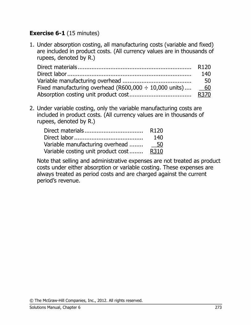
© The McGraw-Hill Companies, Inc., 2012. All rights reserved.
Solutions Manual, Chapter 6 273
Exercise 6-1 (15 minutes)
1. Under absorption costing, all manufacturing costs (variable and fixed) are included in product costs. (All currency values are in thousands of rupees, denoted by R.)
Direct materials .................................................................. R120 Direct labor ........................................................................ 140 Variable manufacturing overhead ........................................ 50 Fixed manufacturing overhead (R600,000 ÷ 10,000 units) .... 60 Absorption costing unit product cost .................................... R370
2. Under variable costing, only the variable manufacturing costs are included in product costs. (All currency values are in thousands of rupees, denoted by R.)
Direct materials .................................. R120 Direct labor ........................................ 140 Variable manufacturing overhead ........ 50 Variable costing unit product cost ........ R310
Note that selling and administrative expenses are not treated as product costs under either absorption or variable costing. These expenses are always treated as period costs and are charged against the current period’s revenue.
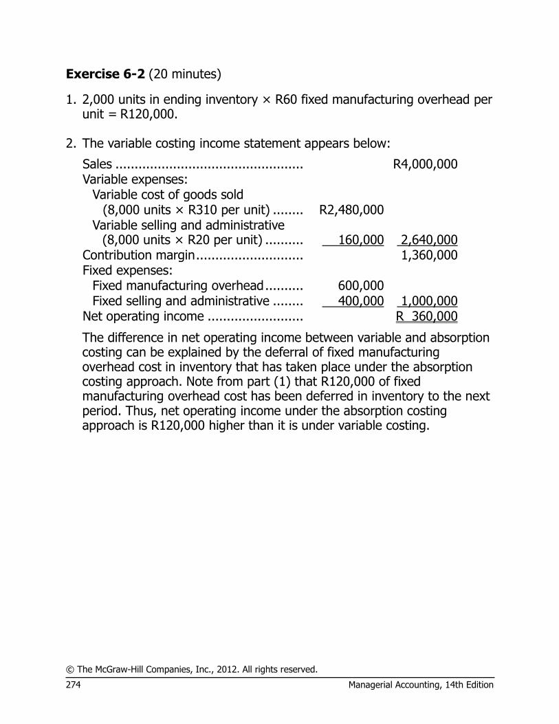
© The McGraw-Hill Companies, Inc., 2012. All rights reserved.
274 Managerial Accounting, 14th Edition
Exercise 6-2 (20 minutes)
1. 2,000 units in ending inventory × R60 fixed manufacturing overhead per unit = R120,000.
2. The variable costing income statement appears below:
Sales ................................................. R4,000,000 Variable expenses:
Variable cost of goods sold (8,000 units × R310 per unit) ........ R2,480,000
Variable selling and administrative (8,000 units × R20 per unit) .......... 160,000 2,640,000
Contribution margin ............................ 1,360,000 Fixed expenses:
Fixed manufacturing overhead .......... 600,000 Fixed selling and administrative ........ 400,000 1,000,000
Net operating income ......................... R 360,000
The difference in net operating income between variable and absorption costing can be explained by the deferral of fixed manufacturing overhead cost in inventory that has taken place under the absorption costing approach. Note from part (1) that R120,000 of fixed manufacturing overhead cost has been deferred in inventory to the next period. Thus, net operating income under the absorption costing approach is R120,000 higher than it is under variable costing.

© The McGraw-Hill Companies, Inc., 2012. All rights reserved.
Solutions Manual, Chapter 6 275
Exercise 6-3 (20 minutes)
1. Year 1 Year 2 Year 3 Beginning inventories .......... 180 150 160 Ending inventories ............... 150 160 200 Change in inventories .......... (30) 10 40
Fixed manufacturing overhead in beginning inventories (@$450 per unit) ................................. $ 81,000 $ 67,500 $72,000
Fixed manufacturing overhead in ending inventories (@$450 per unit) ................................. 67,500 72,000 90,000
Fixed manufacturing overhead deferred in (released from) inventories (@$450 per unit) ................................. $(13,500) $ 4,500 $ 18,000
Variable costing net
operating income .............. $292,400 $269,200 $251,800
Add (deduct) fixed manufacturing overhead cost deferred in (released from) inventory under absorption costing ............ (13,500) 4,500 18,000
Absorption costing net
operating income .............. $278,900 $273,700 $269,800 2. Because absorption costing net operating income was greater than
variable costing net operating income in Year 4, inventories must have increased during the year and hence, fixed manufacturing overhead was deferred in inventories. The amount of the deferral is just the difference between the two net operating incomes or $27,000 = $267,200 – $240,200.
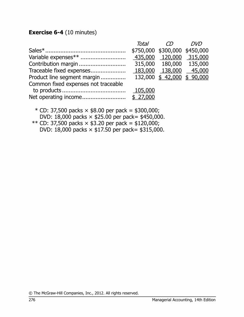
© The McGraw-Hill Companies, Inc., 2012. All rights reserved.
276 Managerial Accounting, 14th Edition
Exercise 6-4 (10 minutes)
Total CD DVD Sales* ................................................ $750,000 $300,000 $450,000 Variable expenses** ........................... 435,000 120,000 315,000 Contribution margin ............................ 315,000 180,000 135,000 Traceable fixed expenses ..................... 183,000 138,000 45,000 Product line segment margin ............... 132,000 $ 42,000 $ 90,000 Common fixed expenses not traceable
to products ...................................... 105,000 Net operating income .......................... $ 27,000
*
**
CD: 37,500 packs × $8.00 per pack = $300,000; DVD: 18,000 packs × $25.00 per pack= $450,000. CD: 37,500 packs × $3.20 per pack = $120,000; DVD: 18,000 packs × $17.50 per pack= $315,000.
© The McGraw-Hill Companies, Inc., 2012. All rights reserved.
Solutions Manual, Chapter 6 277
Exercise 6-5 (10 minutes)
Sales were above the company’s break-even sales and yet the company sustained a loss. The apparent contradiction is explained by the fact that the CVP analysis is based on variable costing, whereas the income reported to shareholders is prepared using absorption costing. Because sales were above the breakeven, the variable costing net operating income would have been positive. However, the absorption costing net operating income was negative. Ordinarily, this would only happen if inventories decreased and fixed manufacturing overhead deferred in inventories was released to the income statement on the absorption costing income statement. This added fixed manufacturing overhead cost resulted in a loss on an absorption costing basis even though the company operated at its breakeven on a variable costing basis.
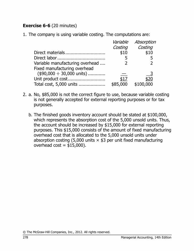
© The McGraw-Hill Companies, Inc., 2012. All rights reserved.
278 Managerial Accounting, 14th Edition
Exercise 6-6 (20 minutes)
1. The company is using variable costing. The computations are:
Variable Costing
Absorption Costing
Direct materials .............................. $10 $10 Direct labor .................................... 5 5 Variable manufacturing overhead .... 2 2 Fixed manufacturing overhead
($90,000 ÷ 30,000 units) ............. — 3 Unit product cost ............................ $17 $20 Total cost, 5,000 units .................... $85,000 $100,000
2. a. No, $85,000 is not the correct figure to use, because variable costing
is not generally accepted for external reporting purposes or for tax purposes.
b. The finished goods inventory account should be stated at $100,000,
which represents the absorption cost of the 5,000 unsold units. Thus, the account should be increased by $15,000 for external reporting purposes. This $15,000 consists of the amount of fixed manufacturing overhead cost that is allocated to the 5,000 unsold units under absorption costing (5,000 units × $3 per unit fixed manufacturing overhead cost = $15,000).
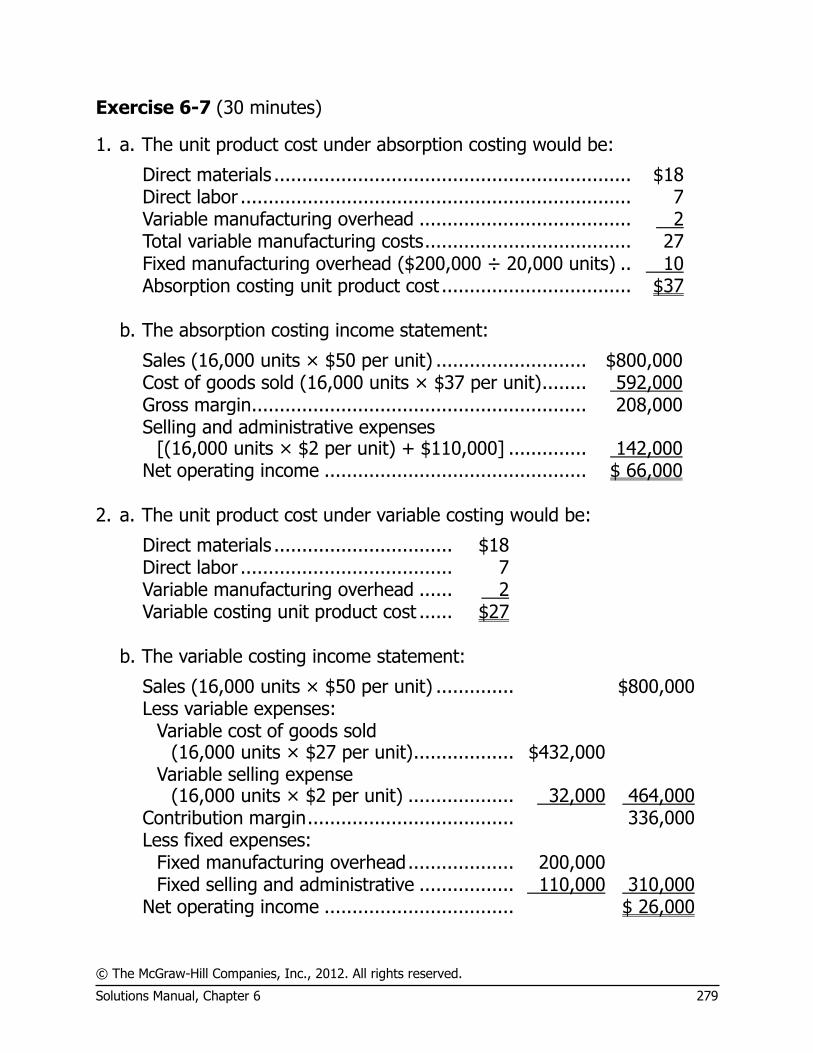
© The McGraw-Hill Companies, Inc., 2012. All rights reserved.
Solutions Manual, Chapter 6 279
Exercise 6-7 (30 minutes)
1. a. The unit product cost under absorption costing would be:
Direct materials ................................................................ $18 Direct labor ...................................................................... 7 Variable manufacturing overhead ...................................... 2 Total variable manufacturing costs ..................................... 27 Fixed manufacturing overhead ($200,000 ÷ 20,000 units) .. 10 Absorption costing unit product cost .................................. $37
b. The absorption costing income statement:
Sales (16,000 units × $50 per unit) ........................... $800,000 Cost of goods sold (16,000 units × $37 per unit) ........ 592,000 Gross margin ............................................................ 208,000 Selling and administrative expenses
[(16,000 units × $2 per unit) + $110,000] .............. 142,000 Net operating income ............................................... $ 66,000
2. a. The unit product cost under variable costing would be:
Direct materials ................................ $18 Direct labor ...................................... 7 Variable manufacturing overhead ...... 2 Variable costing unit product cost ...... $27
b. The variable costing income statement:
Sales (16,000 units × $50 per unit) .............. $800,000 Less variable expenses:
Variable cost of goods sold (16,000 units × $27 per unit) .................. $432,000
Variable selling expense (16,000 units × $2 per unit) ................... 32,000 464,000
Contribution margin ..................................... 336,000 Less fixed expenses:
Fixed manufacturing overhead ................... 200,000 Fixed selling and administrative ................. 110,000 310,000
Net operating income .................................. $ 26,000
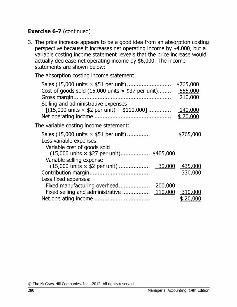
© The McGraw-Hill Companies, Inc., 2012. All rights reserved.
280 Managerial Accounting, 14th Edition
Exercise 6-7 (continued)
3. The price increase appears to be a good idea from an absorption costing perspective because it increases net operating income by $4,000, but a variable costing income statement reveals that the price increase would actually decrease net operating income by $6,000. The income statements are shown below:
The absorption costing income statement:
Sales (15,000 units × $51 per unit) ........................... $765,000 Cost of goods sold (15,000 units × $37 per unit) ........ 555,000 Gross margin ............................................................ 210,000 Selling and administrative expenses
[(15,000 units × $2 per unit) + $110,000] .............. 140,000 Net operating income ............................................... $ 70,000
The variable costing income statement:
Sales (15,000 units × $51 per unit) .............. $765,000 Less variable expenses:
Variable cost of goods sold (15,000 units × $27 per unit) .................. $405,000
Variable selling expense (15,000 units × $2 per unit) ................... 30,000 435,000
Contribution margin ..................................... 330,000 Less fixed expenses:
Fixed manufacturing overhead ................... 200,000 Fixed selling and administrative ................. 110,000 310,000
Net operating income .................................. $ 20,000
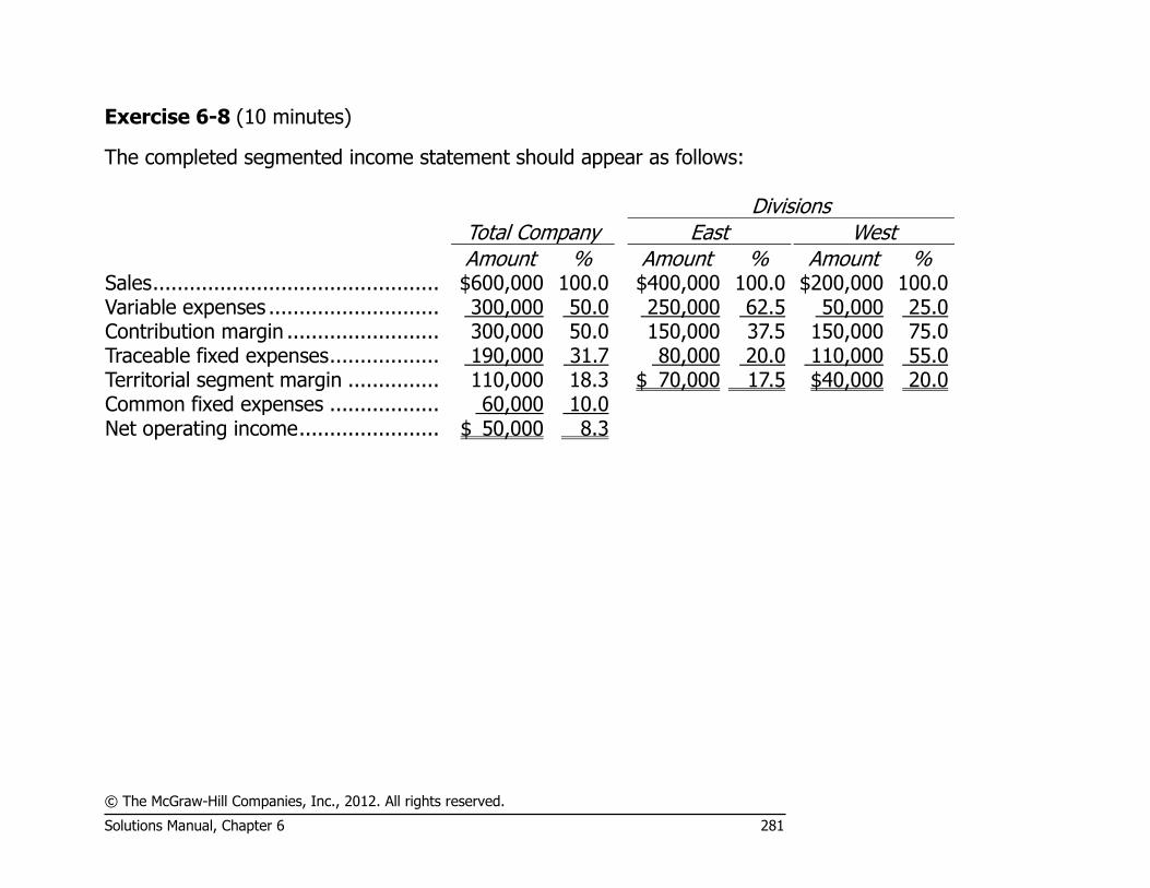
© The McGraw-Hill Companies, Inc., 2012. All rights reserved.
Solutions Manual, Chapter 6 281
Exercise 6-8 (10 minutes)
The completed segmented income statement should appear as follows:
Divisions
Total Company East West
Amount % Amount % Amount % Sales ............................................... $600,000 100.0 $400,000 100.0 $200,000 100.0 Variable expenses ............................ 300,000 50.0 250,000 62.5 50,000 25.0 Contribution margin ......................... 300,000 50.0 150,000 37.5 150,000 75.0 Traceable fixed expenses .................. 190,000 31.7 80,000 20.0 110,000 55.0 Territorial segment margin ............... 110,000 18.3 $ 70,000 17.5 $40,000 20.0 Common fixed expenses .................. 60,000 10.0 Net operating income ....................... $ 50,000 8.3
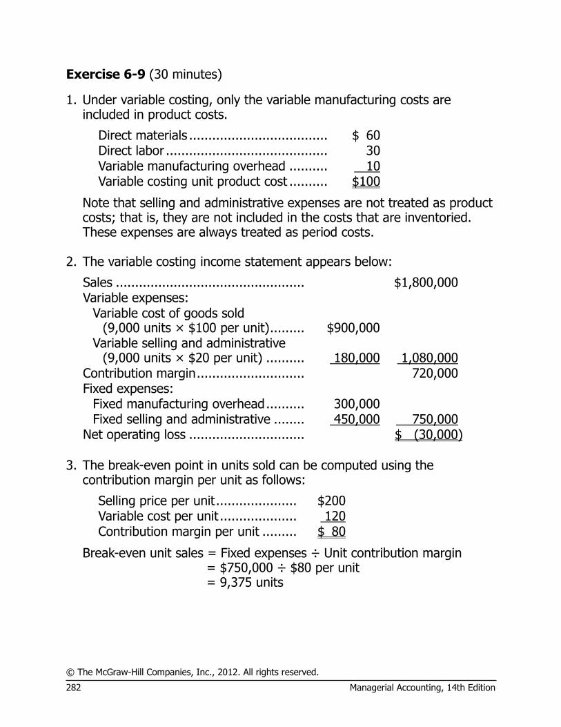
© The McGraw-Hill Companies, Inc., 2012. All rights reserved.
282 Managerial Accounting, 14th Edition
Exercise 6-9 (30 minutes)
1. Under variable costing, only the variable manufacturing costs are included in product costs.
Direct materials .................................... $ 60 Direct labor .......................................... 30 Variable manufacturing overhead .......... 10 Variable costing unit product cost .......... $100
Note that selling and administrative expenses are not treated as product costs; that is, they are not included in the costs that are inventoried. These expenses are always treated as period costs.
2. The variable costing income statement appears below:
Sales ................................................. $1,800,000 Variable expenses:
Variable cost of goods sold (9,000 units × $100 per unit) ......... $900,000
Variable selling and administrative (9,000 units × $20 per unit) .......... 180,000 1,080,000
Contribution margin ............................ 720,000 Fixed expenses:
Fixed manufacturing overhead .......... 300,000 Fixed selling and administrative ........ 450,000 750,000
Net operating loss .............................. $ (30,000)
3. The break-even point in units sold can be computed using the contribution margin per unit as follows:
Selling price per unit ..................... $200 Variable cost per unit .................... 120 Contribution margin per unit ......... $ 80
Break-even unit sales = Fixed expenses ÷ Unit contribution margin = $750,000 ÷ $80 per unit = 9,375 units
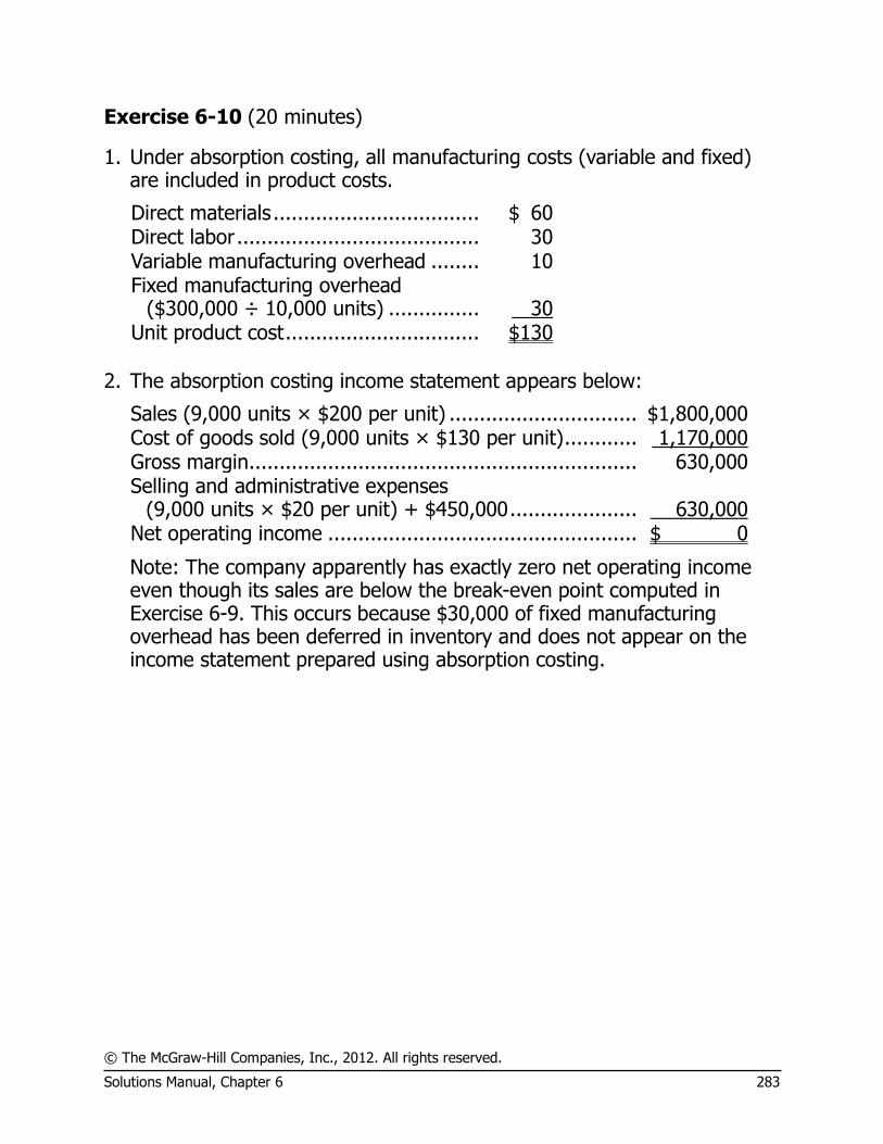
© The McGraw-Hill Companies, Inc., 2012. All rights reserved.
Solutions Manual, Chapter 6 283
Exercise 6-10 (20 minutes)
1. Under absorption costing, all manufacturing costs (variable and fixed) are included in product costs.
Direct materials .................................. $ 60 Direct labor ........................................ 30 Variable manufacturing overhead ........ 10 Fixed manufacturing overhead
($300,000 ÷ 10,000 units) ............... 30 Unit product cost ................................ $130
2. The absorption costing income statement appears below:
Sales (9,000 units × $200 per unit) ............................... $1,800,000 Cost of goods sold (9,000 units × $130 per unit) ............ 1,170,000 Gross margin ................................................................ 630,000 Selling and administrative expenses
(9,000 units × $20 per unit) + $450,000 ..................... 630,000 Net operating income ................................................... $ 0
Note: The company apparently has exactly zero net operating income even though its sales are below the break-even point computed in Exercise 6-9. This occurs because $30,000 of fixed manufacturing overhead has been deferred in inventory and does not appear on the income statement prepared using absorption costing.
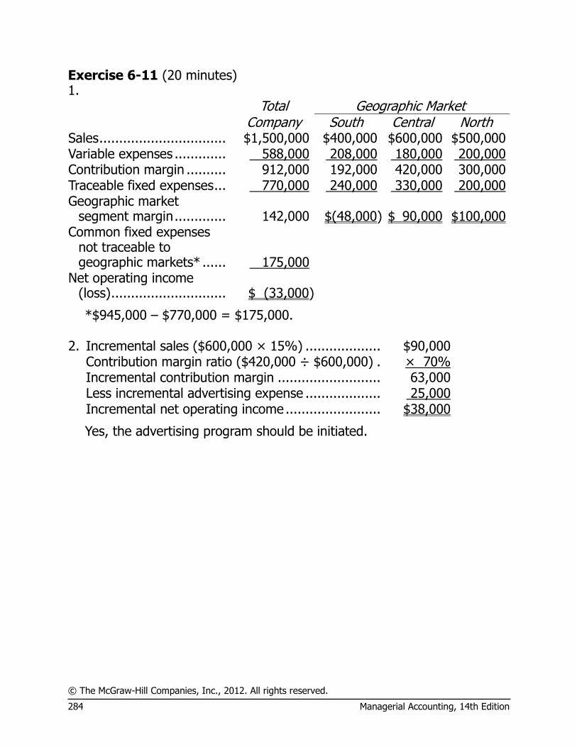
© The McGraw-Hill Companies, Inc., 2012. All rights reserved.
284 Managerial Accounting, 14th Edition
Exercise 6-11 (20 minutes) 1. Total Geographic Market Company South Central North Sales ................................ $1,500,000 $400,000 $600,000 $500,000 Variable expenses ............. 588,000 208,000 180,000 200,000 Contribution margin .......... 912,000 192,000 420,000 300,000 Traceable fixed expenses ... 770,000 240,000 330,000 200,000 Geographic market
segment margin ............. 142,000 $(48,000) $ 90,000 $100,000 Common fixed expenses
not traceable to geographic markets* ...... 175,000
Net operating income (loss) ............................. $ (33,000)
*$945,000 – $770,000 = $175,000. 2. Incremental sales ($600,000 × 15%) ................... $90,000 Contribution margin ratio ($420,000 ÷ $600,000) . × 70% Incremental contribution margin .......................... 63,000 Less incremental advertising expense ................... 25,000 Incremental net operating income ........................ $38,000
Yes, the advertising program should be initiated.

© The McGraw-Hill Companies, Inc., 2012. All rights reserved.
Solutions Manual, Chapter 6 285
Exercise 6-12 (30 minutes)
1 a. Under variable costing, only the variable manufacturing costs are included in product costs.
Year 1 Year 2 Direct materials .................................... $20 $20 Direct labor .......................................... 12 12 Variable manufacturing overhead .......... 4 4 Variable costing unit product cost .......... $36 $36
Note that selling and administrative expenses are not treated as product costs; that is, they are not included in the costs that are inventoried. These expenses are always treated as period costs.
1 b.
Year 1 Year 2 Sales ......................................................... $2,000,000 $2,500,000 Variable expenses:
Variable cost of goods sold @ $36 per unit 1,440,000 1,800,000 Variable selling and administrative @ $3
per unit ................................................ 120,000 150,000 Total variable expenses ............................... 1,560,000 1,950,000 Contribution margin .................................... 440,000 550,000 Fixed expenses:
Fixed manufacturing overhead .................. 200,000 200,000 Fixed selling and administrative ................ 80,000 80,000
Total fixed expenses ................................... 280,000 280,000 Net operating income (loss) ........................ $ 160,000 $ 270,000
2 a. The unit product costs under absorption costing:
Year 1 Year 2 Direct materials .................................... $20 $20 Direct labor .......................................... 12 12 Variable manufacturing overhead .......... 4 4 Fixed manufacturing overhead .............. *4 **5 Absorption costing unit product cost ...... $40 $41
* $200,000 ÷ 50,000 units = $4 per unit. ** $200,000 ÷ 40,000 units = $5 per unit.
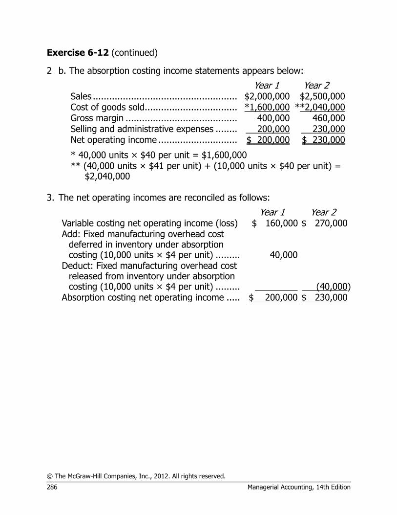
© The McGraw-Hill Companies, Inc., 2012. All rights reserved.
286 Managerial Accounting, 14th Edition
Exercise 6-12 (continued)
2 b. The absorption costing income statements appears below:
Year 1 Year 2 Sales ..................................................... $2,000,000 $2,500,000 Cost of goods sold.................................. *1,600,000 **2,040,000 Gross margin ......................................... 400,000 460,000 Selling and administrative expenses ........ 200,000 230,000 Net operating income ............................. $ 200,000 $ 230,000
* 40,000 units × $40 per unit = $1,600,000 ** (40,000 units × $41 per unit) + (10,000 units × $40 per unit) =
$2,040,000 3. The net operating incomes are reconciled as follows:
Year 1 Year 2 Variable costing net operating income (loss) $ 160,000 $ 270,000 Add: Fixed manufacturing overhead cost
deferred in inventory under absorption costing (10,000 units × $4 per unit) ......... 40,000
Deduct: Fixed manufacturing overhead cost released from inventory under absorption costing (10,000 units × $4 per unit) ......... (40,000)
Absorption costing net operating income ..... $ 200,000 $ 230,000
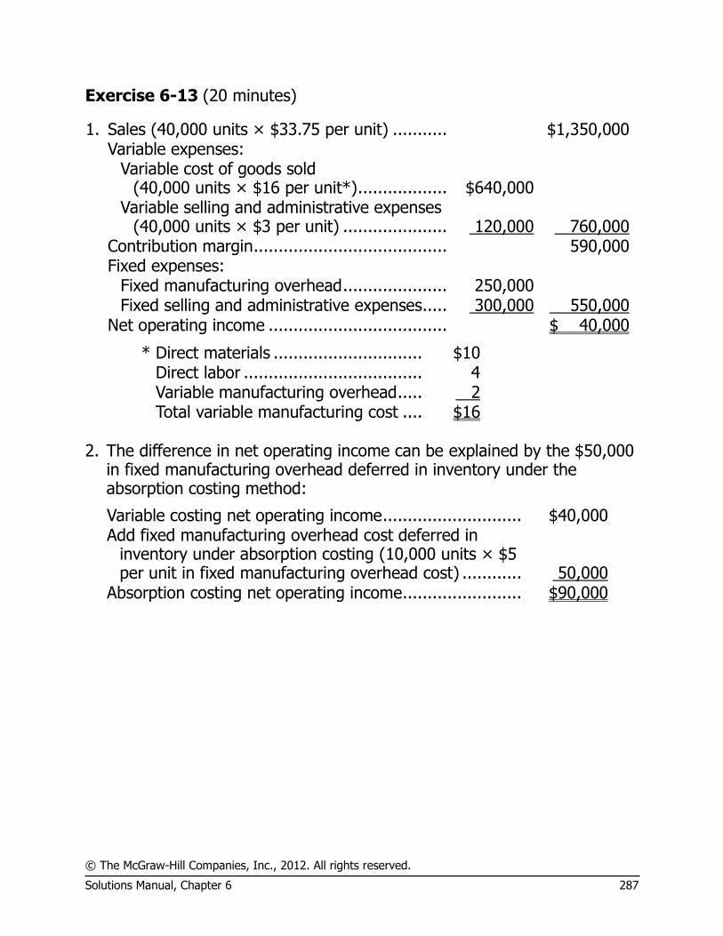
© The McGraw-Hill Companies, Inc., 2012. All rights reserved.
Solutions Manual, Chapter 6 287
Exercise 6-13 (20 minutes)
1. Sales (40,000 units × $33.75 per unit) ........... $1,350,000 Variable expenses:
Variable cost of goods sold
(40,000 units × $16 per unit*) .................. $640,000
Variable selling and administrative expenses
(40,000 units × $3 per unit) ..................... 120,000 760,000 Contribution margin ....................................... 590,000 Fixed expenses: Fixed manufacturing overhead ..................... 250,000 Fixed selling and administrative expenses ..... 300,000 550,000 Net operating income .................................... $ 40,000
* Direct materials .............................. $10 Direct labor .................................... 4 Variable manufacturing overhead ..... 2 Total variable manufacturing cost .... $16
2. The difference in net operating income can be explained by the $50,000
in fixed manufacturing overhead deferred in inventory under the absorption costing method:
Variable costing net operating income ............................ $40,000 Add fixed manufacturing overhead cost deferred in
inventory under absorption costing (10,000 units × $5 per unit in fixed manufacturing overhead cost) ............ 50,000
Absorption costing net operating income ........................ $90,000
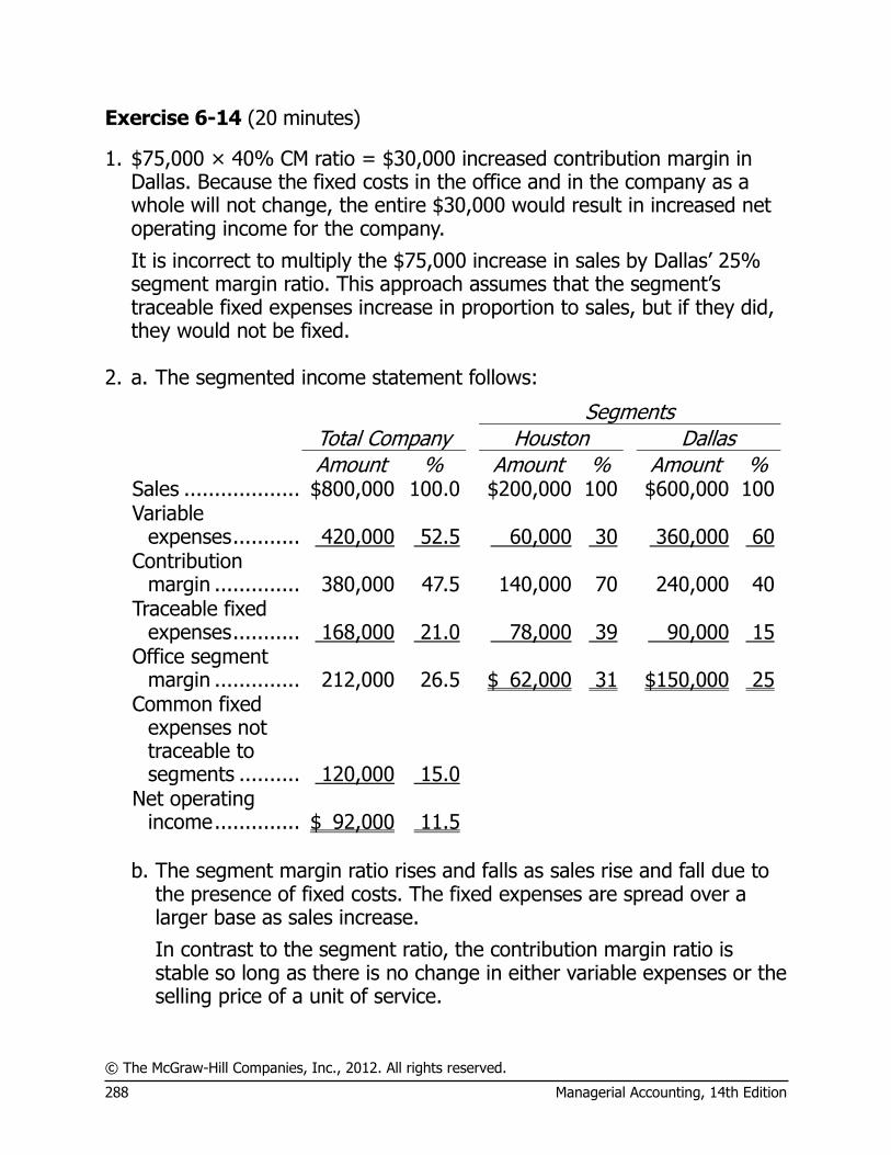
© The McGraw-Hill Companies, Inc., 2012. All rights reserved.
288 Managerial Accounting, 14th Edition
Exercise 6-14 (20 minutes)
1. $75,000 × 40% CM ratio = $30,000 increased contribution margin in Dallas. Because the fixed costs in the office and in the company as a whole will not change, the entire $30,000 would result in increased net operating income for the company.
It is incorrect to multiply the $75,000 increase in sales by Dallas’ 25% segment margin ratio. This approach assumes that the segment’s traceable fixed expenses increase in proportion to sales, but if they did, they would not be fixed.
2. a. The segmented income statement follows:
Segments Total Company Houston Dallas
Amount % Amount % Amount % Sales ....................... $800,000 100.0 $200,000 100 $600,000 100 Variable
expenses ............... 420,000 52.5
60,000 30
360,000 60 Contribution
margin .................. 380,000 47.5
140,000 70
240,000 40 Traceable fixed
expenses ............... 168,000 21.0
78,000 39
90,000 15 Office segment
margin .................. 212,000 26.5
$ 62,000 31
$150,000 25 Common fixed
expenses not traceable to segments .............. 120,000 15.0
Net operating
income .............. $ 92,000 11.5
b. The segment margin ratio rises and falls as sales rise and fall due to the presence of fixed costs. The fixed expenses are spread over a larger base as sales increase.
In contrast to the segment ratio, the contribution margin ratio is stable so long as there is no change in either variable expenses or the selling price of a unit of service.
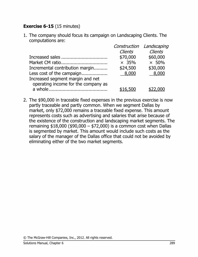
© The McGraw-Hill Companies, Inc., 2012. All rights reserved.
Solutions Manual, Chapter 6 289
Exercise 6-15 (15 minutes)
1. The company should focus its campaign on Landscaping Clients. The computations are:
Construction
Clients Landscaping
Clients Increased sales .................................. $70,000 $60,000 Market CM ratio .................................. × 35% × 50% Incremental contribution margin .......... $24,500 $30,000 Less cost of the campaign ................... 8,000 8,000 Increased segment margin and net
operating income for the company as a whole ........................................... $16,500 $22,000
2. The $90,000 in traceable fixed expenses in the previous exercise is now
partly traceable and partly common. When we segment Dallas by market, only $72,000 remains a traceable fixed expense. This amount represents costs such as advertising and salaries that arise because of the existence of the construction and landscaping market segments. The remaining $18,000 ($90,000 – $72,000) is a common cost when Dallas is segmented by market. This amount would include such costs as the salary of the manager of the Dallas office that could not be avoided by eliminating either of the two market segments.
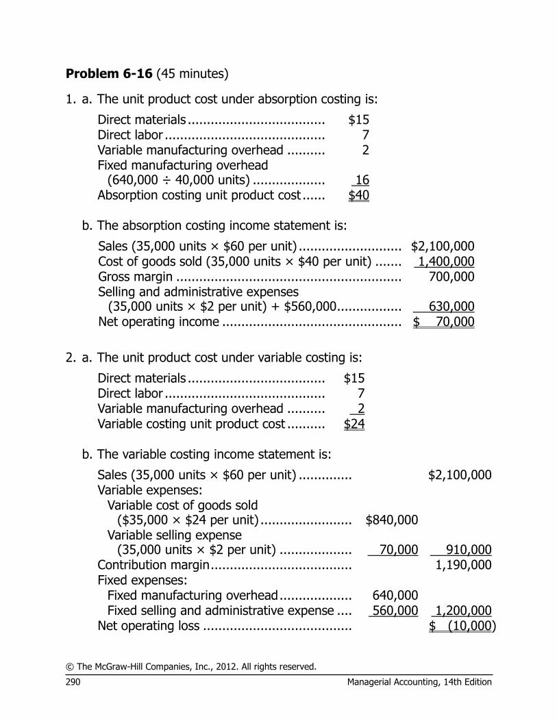
© The McGraw-Hill Companies, Inc., 2012. All rights reserved.
290 Managerial Accounting, 14th Edition
Problem 6-16 (45 minutes)
1. a. The unit product cost under absorption costing is:
Direct materials .................................... $15 Direct labor .......................................... 7 Variable manufacturing overhead .......... 2 Fixed manufacturing overhead
(640,000 ÷ 40,000 units) ................... 16 Absorption costing unit product cost ...... $40
b. The absorption costing income statement is:
Sales (35,000 units × $60 per unit) ........................... $2,100,000 Cost of goods sold (35,000 units × $40 per unit) ....... 1,400,000 Gross margin ........................................................... 700,000
Selling and administrative expenses
(35,000 units × $2 per unit) + $560,000 ................. 630,000 Net operating income ............................................... $ 70,000
2. a. The unit product cost under variable costing is:
Direct materials .................................... $15 Direct labor .......................................... 7 Variable manufacturing overhead .......... 2 Variable costing unit product cost .......... $24
b. The variable costing income statement is:
Sales (35,000 units × $60 per unit) .............. $2,100,000 Variable expenses:
Variable cost of goods sold ($35,000 × $24 per unit) ........................ $840,000
Variable selling expense (35,000 units × $2 per unit) ................... 70,000 910,000
Contribution margin ..................................... 1,190,000 Fixed expenses:
Fixed manufacturing overhead ................... 640,000 Fixed selling and administrative expense .... 560,000 1,200,000
Net operating loss ....................................... $ (10,000)

© The McGraw-Hill Companies, Inc., 2012. All rights reserved.
Solutions Manual, Chapter 6 291
Problem 6-16 (continued)
3. The difference in the ending inventory relates to a difference in the handling of fixed manufacturing overhead costs. Under variable costing, these costs have been expensed in full as period costs. Under absorption costing, these costs have been added to units of product at the rate of $16 per unit ($640,000 ÷ 40,000 units produced = $16 per unit). Thus, under absorption costing a portion of the $640,000 fixed manufacturing overhead cost of the month has been added to the inventory account rather than expensed on the income statement:
Added to the ending inventory (5,000 units × $16 per unit) ....................................... $ 80,000
Expensed as part of cost of goods sold (35,000 units × $16 per unit) ..................................... 560,000
Total fixed manufacturing overhead cost for the month ... $640,000
Because $80,000 of fixed manufacturing overhead cost has been deferred in inventory under absorption costing, the net operating income reported under that costing method is $80,000 higher than the net operating income under variable costing, as shown in parts (1) and (2) above.
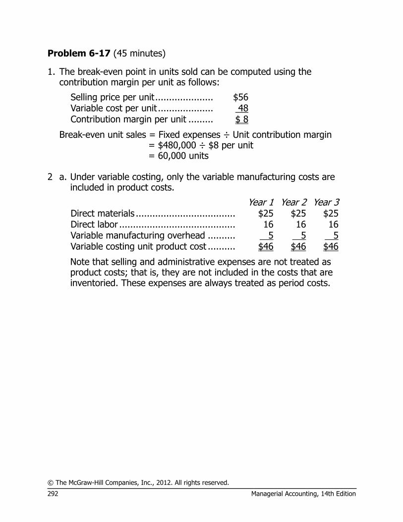
© The McGraw-Hill Companies, Inc., 2012. All rights reserved.
292 Managerial Accounting, 14th Edition
Problem 6-17 (45 minutes)
1. The break-even point in units sold can be computed using the contribution margin per unit as follows:
Selling price per unit ..................... $56 Variable cost per unit .................... 48 Contribution margin per unit ......... $ 8
Break-even unit sales = Fixed expenses ÷ Unit contribution margin = $480,000 ÷ $8 per unit = 60,000 units 2 a. Under variable costing, only the variable manufacturing costs are
included in product costs.
Year 1 Year 2 Year 3 Direct materials .................................... $25 $25 $25 Direct labor .......................................... 16 16 16 Variable manufacturing overhead .......... 5 5 5 Variable costing unit product cost .......... $46 $46 $46
Note that selling and administrative expenses are not treated as product costs; that is, they are not included in the costs that are inventoried. These expenses are always treated as period costs.

© The McGraw-Hill Companies, Inc., 2012. All rights reserved.
Solutions Manual, Chapter 6 293
Problem 6-17 (continued)
2 b. The variable costing income statements appear below:
Year 1 Year 2 Year 3 Sales ........................................................................ $3,360,000 $2,800,000 $3,640,000 Variable expenses:
Variable cost of goods sold @ $46 per unit .............. 2,760,000 2,300,000 2,990,000 Variable selling and administrative @ $2 per unit ..... 120,000 100,000 130,000
Total variable expenses ............................................. 2,880,000 2,400,000 3,120,000 Contribution margin .................................................. 480,000 400,000 520,000 Fixed expenses:
Fixed manufacturing overhead ................................ 300,000 300,000 300,000 Fixed selling and administrative ............................... 180,000 180,000 180,000
Total fixed expenses ................................................. 480,000 480,000 480,000 Net operating income (loss) ...................................... $ 0 $ (80,000) $ 40,000 3 a. The unit product costs under absorption costing:
Year 1 Year 2 Year 3 Direct materials .................................... $25 $25 $25.00 Direct labor .......................................... 16 16 16.00 Variable manufacturing overhead .......... 5 5 5.00 Fixed manufacturing overhead .............. *5 **4 ***7.50 Absorption costing unit product cost ...... $51 $50 $53.50 * $300,000 ÷ 60,000 units = $5 per unit. ** $300,000 ÷ 75,000 units = $4 per unit. *** $300,000 ÷ 40,000 units = $7.50 per unit.
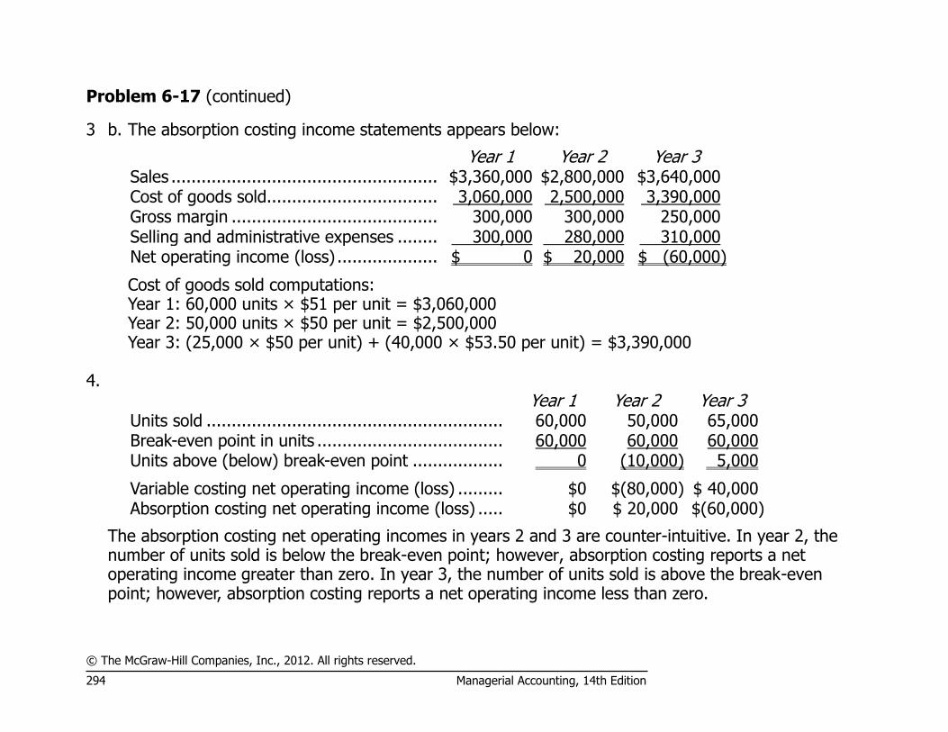
© The McGraw-Hill Companies, Inc., 2012. All rights reserved.
294 Managerial Accounting, 14th Edition
Problem 6-17 (continued)
3 b. The absorption costing income statements appears below:
Year 1 Year 2 Year 3 Sales ..................................................... $3,360,000 $2,800,000 $3,640,000 Cost of goods sold.................................. 3,060,000 2,500,000 3,390,000 Gross margin ......................................... 300,000 300,000 250,000 Selling and administrative expenses ........ 300,000 280,000 310,000 Net operating income (loss) .................... $ 0 $ 20,000 $ (60,000)
Cost of goods sold computations: Year 1: 60,000 units × $51 per unit = $3,060,000 Year 2: 50,000 units × $50 per unit = $2,500,000 Year 3: (25,000 × $50 per unit) + (40,000 × $53.50 per unit) = $3,390,000 4.
Year 1 Year 2 Year 3 Units sold ........................................................... 60,000 50,000 65,000 Break-even point in units ..................................... 60,000 60,000 60,000 Units above (below) break-even point .................. 0 (10,000) 5,000
Variable costing net operating income (loss) ......... $0 $(80,000) $ 40,000 Absorption costing net operating income (loss) ..... $0 $ 20,000 $(60,000)
The absorption costing net operating incomes in years 2 and 3 are counter-intuitive. In year 2, the number of units sold is below the break-even point; however, absorption costing reports a net operating income greater than zero. In year 3, the number of units sold is above the break-even point; however, absorption costing reports a net operating income less than zero.
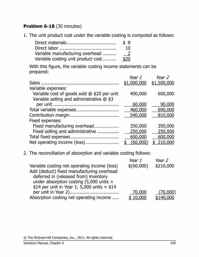
© The McGraw-Hill Companies, Inc., 2012. All rights reserved.
Solutions Manual, Chapter 6 295
Problem 6-18 (30 minutes)
1. The unit product cost under the variable costing is computed as follows:
Direct materials .................................... $ 8 Direct labor .......................................... 10 Variable manufacturing overhead .......... 2 Variable costing unit product cost .......... $20
With this figure, the variable costing income statements can be prepared:
Year 1 Year 2 Sales ......................................................... $1,000,000 $1,500,000 Variable expenses:
Variable cost of goods sold @ $20 per unit 400,000 600,000 Variable selling and administrative @ $3
per unit ................................................ 60,000 90,000 Total variable expenses ............................... 460,000 690,000 Contribution margin .................................... 540,000 810,000 Fixed expenses:
Fixed manufacturing overhead .................. 350,000 350,000 Fixed selling and administrative ................ 250,000 250,000
Total fixed expenses ................................... 600,000 600,000 Net operating income (loss) ........................ $ (60,000) $ 210,000
2. The reconciliation of absorption and variable costing follows:
Year 1 Year 2 Variable costing net operating income (loss) $(60,000) $210,000
Add (deduct) fixed manufacturing overhead deferred in (released from) inventory under absorption costing (5,000 units × $14 per unit in Year 1; 5,000 units × $14 per unit in Year 2) .................................... 70,000 (70,000)
Absorption costing net operating income ..... $ 10,000 $140,000
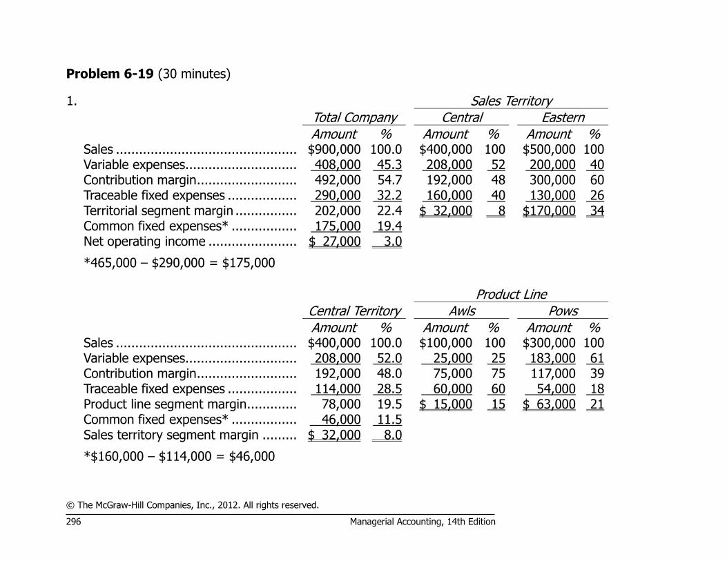
© The McGraw-Hill Companies, Inc., 2012. All rights reserved.
296 Managerial Accounting, 14th Edition
Problem 6-19 (30 minutes)
1. Sales Territory Total Company Central Eastern
Amount % Amount % Amount % Sales ............................................... $900,000 100.0 $400,000 100 $500,000 100 Variable expenses ............................. 408,000 45.3 208,000 52 200,000 40 Contribution margin .......................... 492,000 54.7 192,000 48 300,000 60 Traceable fixed expenses .................. 290,000 32.2 160,000 40 130,000 26 Territorial segment margin ................ 202,000 22.4 $ 32,000 8 $170,000 34 Common fixed expenses* ................. 175,000 19.4 Net operating income ....................... $ 27,000 3.0
*465,000 – $290,000 = $175,000
Product Line
Central Territory Awls Pows
Amount % Amount % Amount % Sales ............................................... $400,000 100.0 $100,000 100 $300,000 100 Variable expenses ............................. 208,000 52.0 25,000 25 183,000 61 Contribution margin .......................... 192,000 48.0 75,000 75 117,000 39 Traceable fixed expenses .................. 114,000 28.5 60,000 60 54,000 18 Product line segment margin ............. 78,000 19.5 $ 15,000 15 $ 63,000 21 Common fixed expenses* ................. 46,000 11.5 Sales territory segment margin ......... $ 32,000 8.0
*$160,000 – $114,000 = $46,000
© The McGraw-Hill Companies, Inc., 2012. All rights reserved.
Solutions Manual, Chapter 6 297
Problem 6-19 (continued)
2. Two points should be brought to the attention of management. First, compared to the Eastern territory, the Central territory has a low contribution margin ratio. Second, the Central territory has high traceable fixed expenses. Overall, compared to the Eastern territory, the Central territory is very weak.
3. Again, two points should be brought to the attention of management.
First, the Central territory has a poor sales mix. Note that the territory sells very little of the Awls product, which has a high contribution margin ratio. It is this poor sales mix that accounts for the low overall contribution margin ratio in the Central territory mentioned in part (2) above. Second, the traceable fixed expenses of the Awls product seem very high in relation to sales. These high fixed expenses may simply mean that the Awls product is highly leveraged; if so, then an increase in sales of this product line would greatly enhance profits in the Central territory and in the company as a whole.
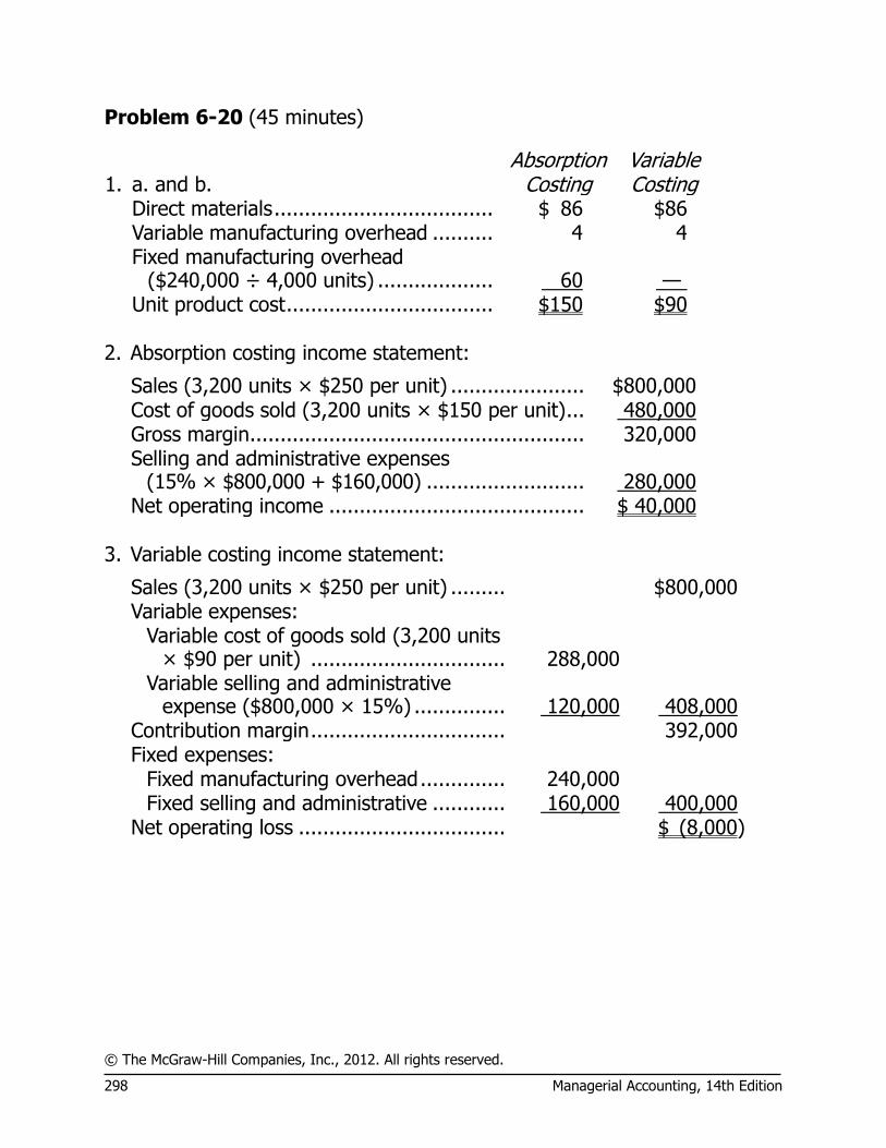
© The McGraw-Hill Companies, Inc., 2012. All rights reserved.
298 Managerial Accounting, 14th Edition
Problem 6-20 (45 minutes)
1. a. and b. Absorption
Costing Variable Costing
Direct materials .................................... $ 86 $86 Variable manufacturing overhead .......... 4 4
Fixed manufacturing overhead
($240,000 ÷ 4,000 units) ................... 60 — Unit product cost .................................. $150 $90 2. Absorption costing income statement:
Sales (3,200 units × $250 per unit) ...................... $800,000 Cost of goods sold (3,200 units × $150 per unit) ... 480,000 Gross margin ....................................................... 320,000 Selling and administrative expenses
(15% × $800,000 + $160,000) .......................... 280,000 Net operating income .......................................... $ 40,000
3. Variable costing income statement:
Sales (3,200 units × $250 per unit) ......... $800,000 Variable expenses:
Variable cost of goods sold (3,200 units × $90 per unit) ................................ 288,000
Variable selling and administrative expense ($800,000 × 15%) ............... 120,000 408,000
Contribution margin ................................ 392,000 Fixed expenses:
Fixed manufacturing overhead .............. 240,000 Fixed selling and administrative ............ 160,000 400,000
Net operating loss .................................. $ (8,000)

© The McGraw-Hill Companies, Inc., 2012. All rights reserved.
Solutions Manual, Chapter 6 299
Problem 6-20 (continued)
4. A manager may prefer to take the statement prepared under the absorption approach in part (2), because it shows a profit for the month. As long as inventory levels are rising, absorption costing will report higher profits than variable costing. Notice in the situation above that the company is operating below its theoretical break-even point [$816,327 = $400,000 ÷ ($392,000/$800,000)], but yet reports a profit under the absorption approach. The ethics of this approach are debatable.
5. Variable costing net operating loss ...................................... $ (8,000)
Add fixed manufacturing overhead cost deferred in inventory under absorption costing (800 units × $60 per unit) ............................................................................... 48,000
Absorption costing net operating income ............................. $40,000

© The McGraw-Hill Companies, Inc., 2012. All rights reserved.
300 Managerial Accounting, 14th Edition
Problem 6-21 (45 minutes)
1. a. and b. Absorption Costing
Variable Costing
Direct materials .................................... $ 6 $ 6 Direct labor .......................................... 12 12 Variable manufacturing overhead .......... 4 4
Fixed manufacturing overhead
($240,000 ÷ 30,000 units) ................. 8 — Unit product cost .................................. $30 $22
2. May June Sales .......................................................... $1,040,000 $1,360,000 Variable expenses: Variable cost of goods sold @ $22 per unit . 572,000 748,000
Variable selling and administrative expense
@ $3 per unit ........................................ 78,000 102,000 Total variable expenses ................................ 650,000 850,000 Contribution margin ..................................... 390,000 510,000 Fixed expenses: Fixed manufacturing overhead ................... 240,000 240,000 Fixed selling and administrative expenses ... 180,000 180,000 Total fixed expenses .................................... 420,000 420,000 Net operating income (loss) ......................... $ (30,000) $ 90,000
3. May June Variable costing net operating income (loss) $ (30,000) $ 90,000
Add fixed manufacturing overhead cost deferred in inventory under absorption costing (4,000 units × $8 per unit) ........... 32,000
Deduct fixed manufacturing overhead cost released from inventory under absorption costing (4,000 units × $8 per unit) ........... (32,000)
Absorption costing net operating income ..... $ 2,000 $ 58,000

© The McGraw-Hill Companies, Inc., 2012. All rights reserved.
Solutions Manual, Chapter 6 301
Problem 6-21 (continued)
4. As shown in the reconciliation in part (3) above, $32,000 of fixed manufacturing overhead cost was deferred in inventory under absorption costing at the end of May, because $8 of fixed manufacturing overhead cost ―attached‖ to each of the 4,000 unsold units that went into inventory at the end of that month. This $32,000 was part of the $420,000 total fixed cost that has to be covered each month in order for the company to break even. Because the $32,000 was added to the inventory account, and thus did not appear on the income statement for May as an expense, the company was able to report a small profit for the month even though it sold less than the break-even volume of sales. In short, only $388,000 of fixed cost ($420,000 – $32,000) was expensed for May, rather than the full $420,000, as contemplated in the break-even analysis. As stated in the text, this is a major problem with the use of absorption costing internally for management purposes. The method does not harmonize well with the principles of cost-volume-profit analysis, and can result in data that are unclear or confusing.

© The McGraw-Hill Companies, Inc., 2012. All rights reserved.
302 Managerial Accounting, 14th Edition
Problem 6-22 (60 minutes)
1. a. Absorption costing unit product cost is:
Direct materials ........................................... $1.00
Direct labor ................................................. 0.80 Variable manufacturing overhead ................. 0.20
Fixed manufacturing overhead
($75,000 ÷ 50,000 units) .......................... 1.50 Absorption costing unit product cost ............. $3.50 b. The absorption costing income statement is:
Sales (40,000 units) ................................................. $200,000 Cost of goods sold (40,000 units × $3.50 per unit) .... 140,000 Gross margin ........................................................... 60,000
Selling and administrative expenses
($20,000 + 40,000 units × $0.75 per unit) .............. 50,000 Net operating income ............................................... $ 10,000
c. The reconciliation is as follows:
Variable costing net operating loss ............................ $ (5,000)
Add fixed manufacturing overhead cost deferred in inventory under absorption costing (10,000 units × $1.50 per unit) .............................. 15,000
Absorption costing net operating income ................... $ 10,000
2. Under absorption costing, the company did earn a profit for the month. However, before the question can really be answered, one must first define what is meant by a ―profit.‖ The central issue here relates to timing of release of fixed manufacturing overhead costs to expense. Advocates of variable costing would argue that all such costs should be expensed immediately, and that no profit is earned unless the revenues of a period are sufficient to cover the fixed manufacturing overhead costs in full. From this point of view, then, no profit was earned during the month, because the fixed costs were not fully covered.

© The McGraw-Hill Companies, Inc., 2012. All rights reserved.
Solutions Manual, Chapter 6 303
Problem 6-22 (continued)
Advocates of absorption costing would argue, however, that fixed manufacturing overhead costs attach to units of product as they are produced, and that such costs do not become expense until the units are sold. Therefore, if the selling price of a unit is greater than the unit cost (including a proportionate amount of fixed manufacturing overhead), then a profit is earned even if some units produced are unsold and carry some fixed manufacturing overhead with them to the following period. A difficulty with this argument is that ―profits‖ will vary under absorption costing depending on how many units are added to or taken out of inventory. That is, profits will depend not only on sales, but on what happens to inventories. In particular, profits can be consciously manipulated by increasing or decreasing a company’s inventories.
3. a. The variable costing income statement is:
Sales (60,000 units × $5 per unit) .................. $300,000 Variable expenses:
Variable cost of goods sold
(60,000 units × $2 per unit) ..................... $120,000
Variable selling and administrative expenses
(60,000 units × $0.75 per unit)................. 45,000 165,000 Contribution margin ...................................... 135,000 Fixed expense: Fixed manufacturing overhead..................... 75,000 Fixed selling and administrative expense ...... 20,000 95,000 Net operating income .................................... $ 40,000
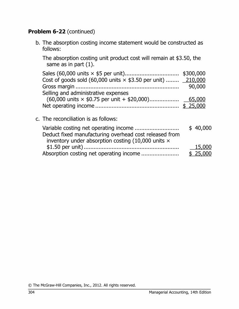
© The McGraw-Hill Companies, Inc., 2012. All rights reserved.
304 Managerial Accounting, 14th Edition
Problem 6-22 (continued)
b. The absorption costing income statement would be constructed as
follows:
The absorption costing unit product cost will remain at $3.50, the
same as in part (1).
Sales (60,000 units × $5 per unit) ................................. $300,000 Cost of goods sold (60,000 units × $3.50 per unit) ........ 210,000 Gross margin ............................................................... 90,000
Selling and administrative expenses
(60,000 units × $0.75 per unit + $20,000) .................. 65,000 Net operating income ................................................... $ 25,000 c. The reconciliation is as follows:
Variable costing net operating income ........................... $ 40,000
Deduct fixed manufacturing overhead cost released from inventory under absorption costing (10,000 units × $1.50 per unit) .......................................................... 15,000
Absorption costing net operating income ....................... $ 25,000

© The McGraw-Hill Companies, Inc., 2012. All rights reserved.
Solutions Manual, Chapter 6 305
Problem 6-23 (60 minutes)
1. The disadvantages or weaknesses of the company’s version of a segmented income statement are as follows:
a. The company should include a column showing the combined results of the three territories taken together.
b. The territorial expenses should be segregated into variable and fixed categories to permit the computation of both a contribution margin and a territorial segment margin.
c. The corporate expenses are probably common to the territories and should not be allocated.
2. Corporate advertising expenses have apparently been allocated on the
basis of sales dollars; the general administrative expenses have apparently been allocated evenly among the three territories. Such allocations can be misleading to management because they seem to imply that these expenses are caused by the segments to which they have been allocated. The segment margin—which only includes costs that are actually caused by the segments—should be used to measure the performance of a segment. The ―net operating income‖ or ―net loss‖ after allocating common expenses should not be used to judge the performance of a segment.
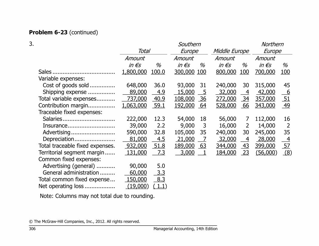
© The McGraw-Hill Companies, Inc., 2012. All rights reserved.
306 Managerial Accounting, 14th Edition
Problem 6-23 (continued)
3.
Total Southern Europe Middle Europe
Northern Europe
Amount
in €s % Amount
in €s % Amount
in €s % Amount
in €s % Sales ..................................... 1,800,000 100.0 300,000 100 800,000 100 700,000 100 Variable expenses: Cost of goods sold ............... 648,000 36.0 93,000 31 240,000 30 315,000 45 Shipping expense ................ 89,000 4.9 15,000 5 32,000 4 42,000 6 Total variable expenses ........... 737,000 40.9 108,000 36 272,000 34 357,000 51 Contribution margin................ 1,063,000 59.1 192,000 64 528,000 66 343,000 49 Traceable fixed expenses: Salaries ............................... 222,000 12.3 54,000 18 56,000 7 112,000 16 Insurance ............................ 39,000 2.2 9,000 3 16,000 2 14,000 2 Advertising .......................... 590,000 32.8 105,000 35 240,000 30 245,000 35 Depreciation ........................ 81,000 4.5 21,000 7 32,000 4 28,000 4 Total traceable fixed expenses . 932,000 51.8 189,000 63 344,000 43 399,000 57 Territorial segment margin ...... 131,000 7.3 3,000 1 184,000 23 (56,000) (8) Common fixed expenses: Advertising (general) ........... 90,000 5.0 General administration ......... 60,000 3.3 Total common fixed expense ... 150,000 8.3 Net operating loss .................. (19,000) ( 1.1)
Note: Columns may not total due to rounding.

© The McGraw-Hill Companies, Inc., 2012. All rights reserved.
Solutions Manual, Chapter 6 307
Problem 6-23 (continued)
4. The following points should be brought to the attention of management:
a. Sales in Southern Europe are much lower than in the other two territories. This is not due to lack of salespeople—salaries in Southern Europe are about the same as in Middle Europe, which has the highest sales of the three territories.
b. Southern Europe is spending less than half as much for advertising as Middle Europe. Perhaps this is the reason for Southern Europe’s lower sales.
c. Northern Europe has a poor sales mix; apparently it is selling a large amount of low-margin items. Note that its contribution margin ratio is only 49%, as compared to 64% or more for the other two territories.
d. Northern Europe may be overstaffed. Its total salaries are much higher than in either of the other two territories.
e. Northern Europe is not covering its own traceable costs. Attention should be given to changing the sales mix and reducing expenses in this territory.
f. Apparently, the salespeople in all three territories are on a salary basis. Perhaps a change to a commission basis would encourage the sales staff to be more aggressive and improve sales throughout the company.
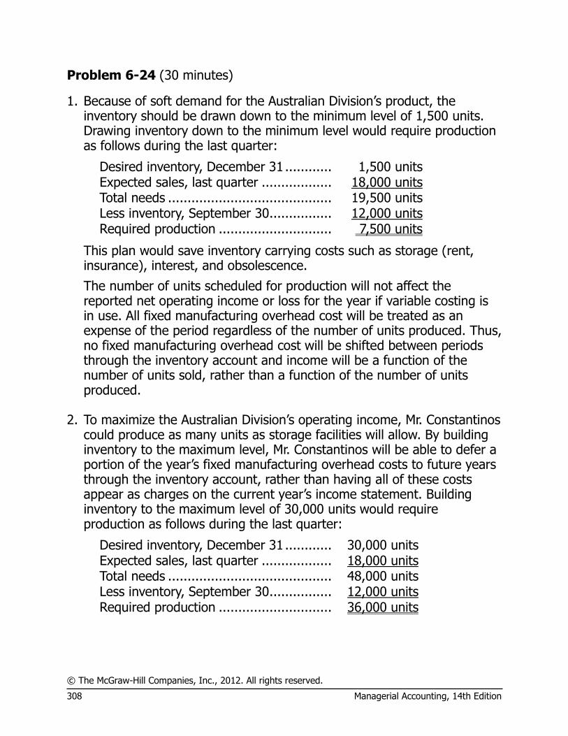
© The McGraw-Hill Companies, Inc., 2012. All rights reserved.
308 Managerial Accounting, 14th Edition
Problem 6-24 (30 minutes)
1. Because of soft demand for the Australian Division’s product, the inventory should be drawn down to the minimum level of 1,500 units. Drawing inventory down to the minimum level would require production as follows during the last quarter:
Desired inventory, December 31 ............ 1,500 units Expected sales, last quarter .................. 18,000 units Total needs .......................................... 19,500 units Less inventory, September 30 ................ 12,000 units Required production ............................. 7,500 units
This plan would save inventory carrying costs such as storage (rent, insurance), interest, and obsolescence.
The number of units scheduled for production will not affect the reported net operating income or loss for the year if variable costing is in use. All fixed manufacturing overhead cost will be treated as an expense of the period regardless of the number of units produced. Thus, no fixed manufacturing overhead cost will be shifted between periods through the inventory account and income will be a function of the number of units sold, rather than a function of the number of units produced.
2. To maximize the Australian Division’s operating income, Mr. Constantinos
could produce as many units as storage facilities will allow. By building inventory to the maximum level, Mr. Constantinos will be able to defer a portion of the year’s fixed manufacturing overhead costs to future years through the inventory account, rather than having all of these costs appear as charges on the current year’s income statement. Building inventory to the maximum level of 30,000 units would require production as follows during the last quarter:
Desired inventory, December 31 ............ 30,000 units Expected sales, last quarter .................. 18,000 units Total needs .......................................... 48,000 units Less inventory, September 30 ................ 12,000 units Required production ............................. 36,000 units
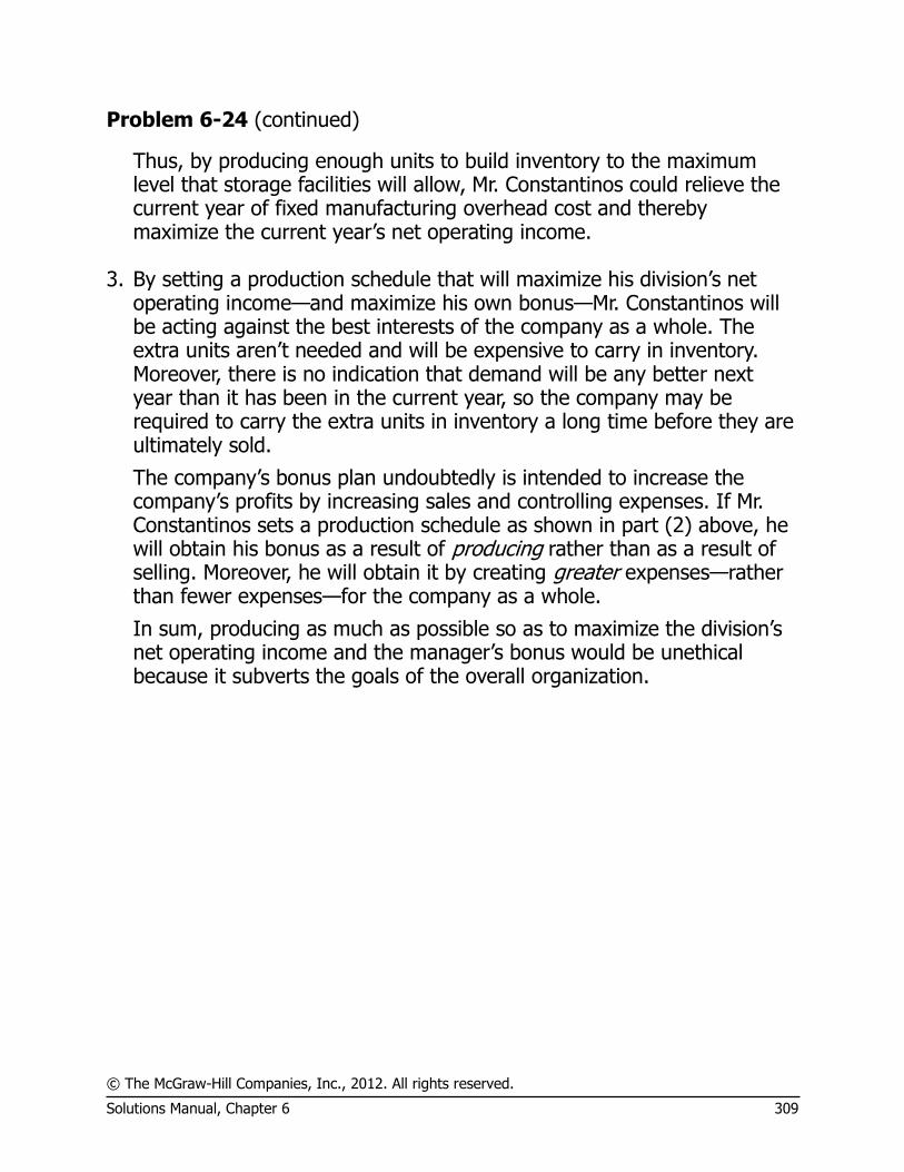
© The McGraw-Hill Companies, Inc., 2012. All rights reserved.
Solutions Manual, Chapter 6 309
Problem 6-24 (continued)
Thus, by producing enough units to build inventory to the maximum level that storage facilities will allow, Mr. Constantinos could relieve the current year of fixed manufacturing overhead cost and thereby maximize the current year’s net operating income.
3. By setting a production schedule that will maximize his division’s net
operating income—and maximize his own bonus—Mr. Constantinos will be acting against the best interests of the company as a whole. The extra units aren’t needed and will be expensive to carry in inventory. Moreover, there is no indication that demand will be any better next year than it has been in the current year, so the company may be required to carry the extra units in inventory a long time before they are ultimately sold.
The company’s bonus plan undoubtedly is intended to increase the company’s profits by increasing sales and controlling expenses. If Mr. Constantinos sets a production schedule as shown in part (2) above, he will obtain his bonus as a result of producing rather than as a result of selling. Moreover, he will obtain it by creating greater expenses—rather than fewer expenses—for the company as a whole.
In sum, producing as much as possible so as to maximize the division’s net operating income and the manager’s bonus would be unethical because it subverts the goals of the overall organization.
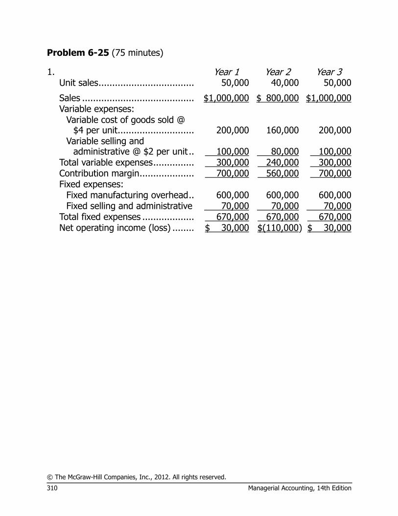
© The McGraw-Hill Companies, Inc., 2012. All rights reserved.
310 Managerial Accounting, 14th Edition
Problem 6-25 (75 minutes)
1. Year 1 Year 2 Year 3 Unit sales ................................... 50,000 40,000 50,000
Sales ......................................... $1,000,000 $ 800,000 $1,000,000 Variable expenses:
Variable cost of goods sold @
$4 per unit ............................ 200,000 160,000 200,000
Variable selling and
administrative @ $2 per unit .. 100,000 80,000 100,000 Total variable expenses ............... 300,000 240,000 300,000 Contribution margin .................... 700,000 560,000 700,000 Fixed expenses: Fixed manufacturing overhead .. 600,000 600,000 600,000 Fixed selling and administrative 70,000 70,000 70,000 Total fixed expenses ................... 670,000 670,000 670,000 Net operating income (loss) ........ $ 30,000 $(110,000) $ 30,000
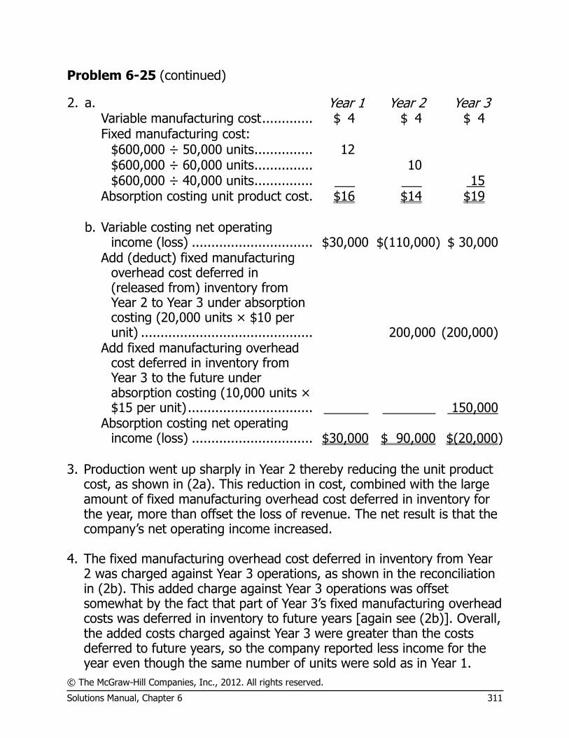
© The McGraw-Hill Companies, Inc., 2012. All rights reserved.
Solutions Manual, Chapter 6 311
Problem 6-25 (continued)
2. a. Year 1 Year 2 Year 3 Variable manufacturing cost ............. $ 4 $ 4 $ 4 Fixed manufacturing cost: $600,000 ÷ 50,000 units ............... 12 $600,000 ÷ 60,000 units ............... 10 $600,000 ÷ 40,000 units ............... 15 Absorption costing unit product cost . $16 $14 $19 b. Variable costing net operating
income (loss) ............................... $30,000 $(110,000) $ 30,000
Add (deduct) fixed manufacturing overhead cost deferred in (released from) inventory from Year 2 to Year 3 under absorption costing (20,000 units × $10 per unit) ............................................ 200,000 (200,000)
Add fixed manufacturing overhead cost deferred in inventory from Year 3 to the future under absorption costing (10,000 units × $15 per unit) ................................ 150,000
Absorption costing net operating
income (loss) ............................... $30,000 $ 90,000 $(20,000) 3. Production went up sharply in Year 2 thereby reducing the unit product
cost, as shown in (2a). This reduction in cost, combined with the large amount of fixed manufacturing overhead cost deferred in inventory for the year, more than offset the loss of revenue. The net result is that the company’s net operating income increased.
4. The fixed manufacturing overhead cost deferred in inventory from Year
2 was charged against Year 3 operations, as shown in the reconciliation in (2b). This added charge against Year 3 operations was offset somewhat by the fact that part of Year 3’s fixed manufacturing overhead costs was deferred in inventory to future years [again see (2b)]. Overall, the added costs charged against Year 3 were greater than the costs deferred to future years, so the company reported less income for the year even though the same number of units were sold as in Year 1.
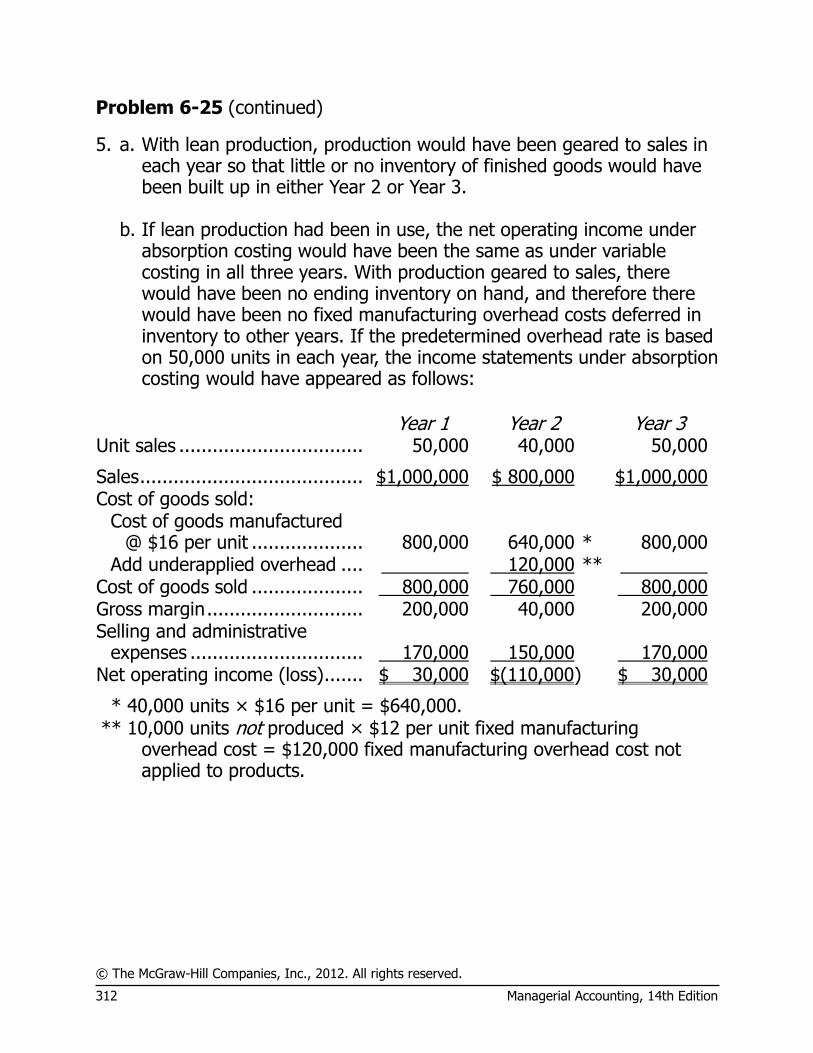
© The McGraw-Hill Companies, Inc., 2012. All rights reserved.
312 Managerial Accounting, 14th Edition
Problem 6-25 (continued)
5. a. With lean production, production would have been geared to sales in each year so that little or no inventory of finished goods would have been built up in either Year 2 or Year 3.
b. If lean production had been in use, the net operating income under
absorption costing would have been the same as under variable costing in all three years. With production geared to sales, there would have been no ending inventory on hand, and therefore there would have been no fixed manufacturing overhead costs deferred in inventory to other years. If the predetermined overhead rate is based on 50,000 units in each year, the income statements under absorption costing would have appeared as follows:
Year 1 Year 2 Year 3 Unit sales ................................. 50,000 40,000 50,000
Sales ........................................ $1,000,000 $ 800,000 $1,000,000 Cost of goods sold:
Cost of goods manufactured @ $16 per unit .................... 800,000 640,000 * 800,000
Add underapplied overhead .... 120,000 ** Cost of goods sold .................... 800,000 760,000 800,000 Gross margin ............................ 200,000 40,000 200,000 Selling and administrative
expenses ............................... 170,000 150,000 170,000 Net operating income (loss) ....... $ 30,000 $(110,000) $ 30,000
* 40,000 units × $16 per unit = $640,000. ** 10,000 units not produced × $12 per unit fixed manufacturing
overhead cost = $120,000 fixed manufacturing overhead cost not applied to products.

© The McGraw-Hill Companies, Inc., 2012. All rights reserved.
Solutions Manual, Chapter 6 313
Problem 6-26 (45 minutes)
1. The segmented income statement follows:
Total
Company Wheat Cereal
Pancake Mix Flour
Sales ................................ $600,000 $200,000 $300,000 $100,000 Variable expenses:
Materials, labor & other ... 204,000 60,000 126,000 18,000 Sales commissions .......... 60,000 20,000 30,000 10,000
Total variable expenses ...... 264,000 80,000 156,000 28,000 Contribution margin ........... 336,000 120,000 144,000 72,000 Traceable fixed expenses:
Advertising ..................... 123,000 48,000 60,000 15,000 Salaries .......................... 66,000 34,000 21,000 11,000 Equipment depreciation* . 30,000 12,000 15,000 3,000 Warehouse rent** .......... 12,000 4,000 7,000 1,000
Total traceable fixed expenses ........................ 231,000 98,000 103,000 30,000
Product line segment margin ........................... 105,000 $ 22,000 $ 41,000 $ 42,000
Common fixed expenses: General administration .... 90,000
Net operating income ........ $ 15,000
* $30,000 × 40%, 50%, and 10% respectively ** $0.50 per square foot × 8,000 square feet, 14,000 square feet, and
2,000 square feet respectively
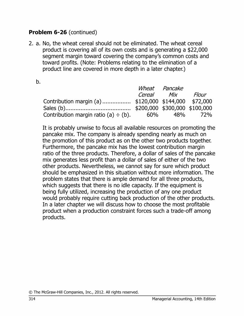
© The McGraw-Hill Companies, Inc., 2012. All rights reserved.
314 Managerial Accounting, 14th Edition
Problem 6-26 (continued)
2. a. No, the wheat cereal should not be eliminated. The wheat cereal product is covering all of its own costs and is generating a $22,000 segment margin toward covering the company’s common costs and toward profits. (Note: Problems relating to the elimination of a product line are covered in more depth in a later chapter.)
b.
Wheat Cereal
Pancake Mix Flour
Contribution margin (a) ................. $120,000 $144,000 $72,000 Sales (b) ....................................... $200,000 $300,000 $100,000 Contribution margin ratio (a) ÷ (b) . 60% 48% 72%
It is probably unwise to focus all available resources on promoting the
pancake mix. The company is already spending nearly as much on the promotion of this product as on the other two products together. Furthermore, the pancake mix has the lowest contribution margin ratio of the three products. Therefore, a dollar of sales of the pancake mix generates less profit than a dollar of sales of either of the two other products. Nevertheless, we cannot say for sure which product should be emphasized in this situation without more information. The problem states that there is ample demand for all three products, which suggests that there is no idle capacity. If the equipment is being fully utilized, increasing the production of any one product would probably require cutting back production of the other products. In a later chapter we will discuss how to choose the most profitable product when a production constraint forces such a trade-off among products.
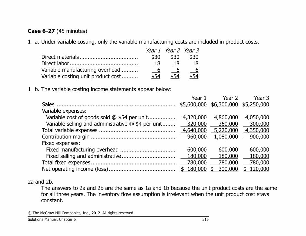
© The McGraw-Hill Companies, Inc., 2012. All rights reserved.
Solutions Manual, Chapter 6 315
Case 6-27 (45 minutes)
1 a. Under variable costing, only the variable manufacturing costs are included in product costs.
Year 1 Year 2 Year 3 Direct materials .................................... $30 $30 $30 Direct labor .......................................... 18 18 18 Variable manufacturing overhead .......... 6 6 6 Variable costing unit product cost .......... $54 $54 $54
1 b. The variable costing income statements appear below:
Year 1 Year 2 Year 3 Sales ........................................................................... $5,600,000 $6,300,000 $5,250,000 Variable expenses:
Variable cost of goods sold @ $54 per unit .................. 4,320,000 4,860,000 4,050,000 Variable selling and administrative @ $4 per unit ......... 320,000 360,000 300,000
Total variable expenses ................................................ 4,640,000 5,220,000 4,350,000 Contribution margin ..................................................... 960,000 1,080,000 900,000 Fixed expenses:
Fixed manufacturing overhead ................................... 600,000 600,000 600,000 Fixed selling and administrative .................................. 180,000 180,000 180,000
Total fixed expenses ..................................................... 780,000 780,000 780,000 Net operating income (loss) .......................................... $ 180,000 $ 300,000 $ 120,000
2a and 2b. The answers to 2a and 2b are the same as 1a and 1b because the unit product costs are the same
for all three years. The inventory flow assumption is irrelevant when the unit product cost stays constant.
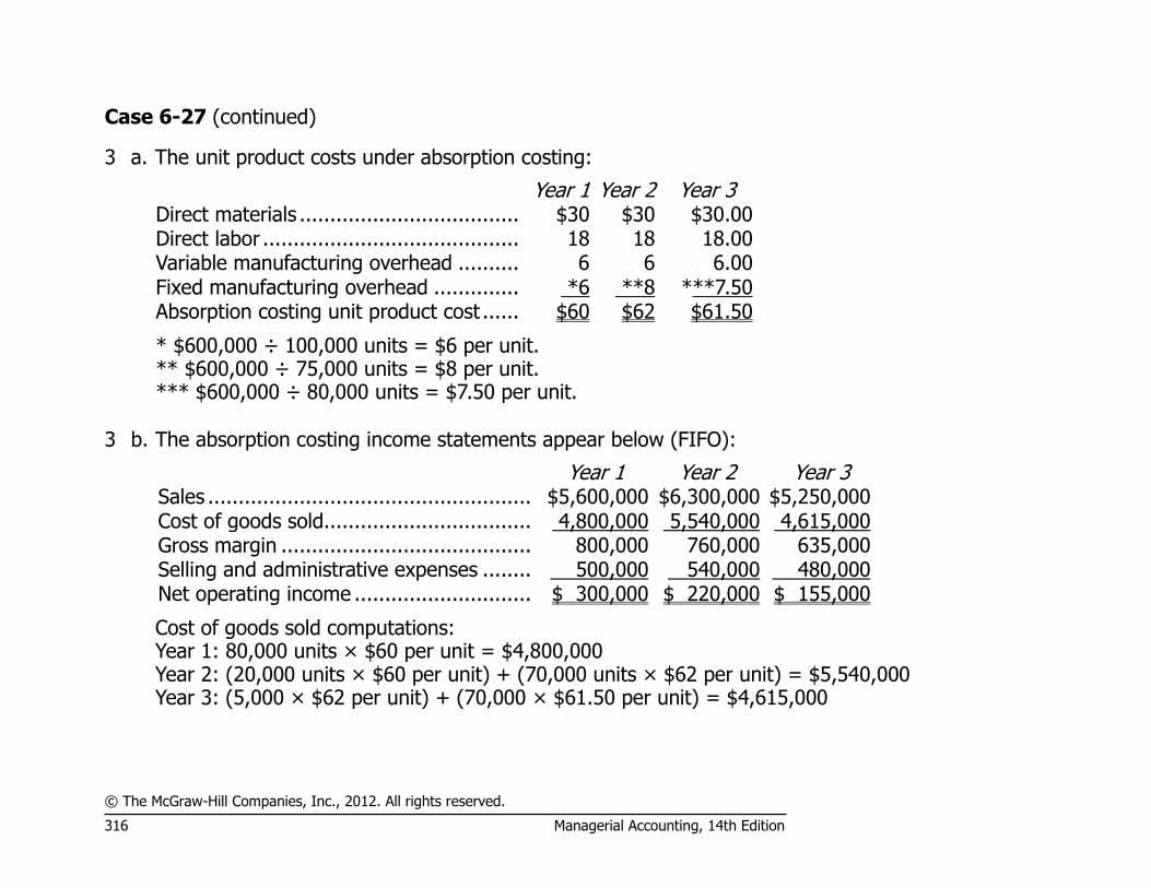
© The McGraw-Hill Companies, Inc., 2012. All rights reserved.
316 Managerial Accounting, 14th Edition
Case 6-27 (continued)
3 a. The unit product costs under absorption costing:
Year 1 Year 2 Year 3 Direct materials .................................... $30 $30 $30.00 Direct labor .......................................... 18 18 18.00 Variable manufacturing overhead .......... 6 6 6.00 Fixed manufacturing overhead .............. *6 **8 ***7.50 Absorption costing unit product cost ...... $60 $62 $61.50
* $600,000 ÷ 100,000 units = $6 per unit. ** $600,000 ÷ 75,000 units = $8 per unit. *** $600,000 ÷ 80,000 units = $7.50 per unit.
3 b. The absorption costing income statements appear below (FIFO):
Year 1 Year 2 Year 3 Sales ..................................................... $5,600,000 $6,300,000 $5,250,000 Cost of goods sold.................................. 4,800,000 5,540,000 4,615,000 Gross margin ......................................... 800,000 760,000 635,000 Selling and administrative expenses ........ 500,000 540,000 480,000 Net operating income ............................. $ 300,000 $ 220,000 $ 155,000
Cost of goods sold computations: Year 1: 80,000 units × $60 per unit = $4,800,000 Year 2: (20,000 units × $60 per unit) + (70,000 units × $62 per unit) = $5,540,000 Year 3: (5,000 × $62 per unit) + (70,000 × $61.50 per unit) = $4,615,000
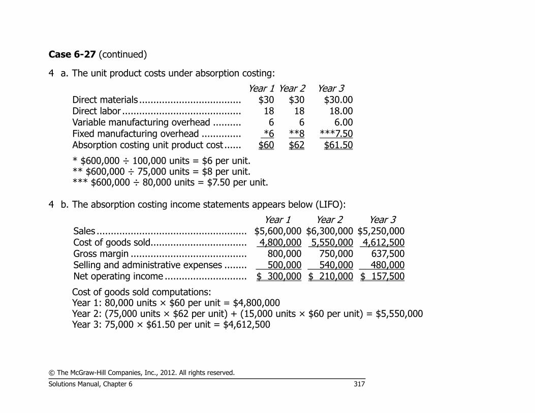
© The McGraw-Hill Companies, Inc., 2012. All rights reserved.
Solutions Manual, Chapter 6 317
Case 6-27 (continued)
4 a. The unit product costs under absorption costing:
Year 1 Year 2 Year 3 Direct materials .................................... $30 $30 $30.00 Direct labor .......................................... 18 18 18.00 Variable manufacturing overhead .......... 6 6 6.00 Fixed manufacturing overhead .............. *6 **8 ***7.50 Absorption costing unit product cost ...... $60 $62 $61.50
* $600,000 ÷ 100,000 units = $6 per unit. ** $600,000 ÷ 75,000 units = $8 per unit. *** $600,000 ÷ 80,000 units = $7.50 per unit.
4 b. The absorption costing income statements appears below (LIFO):
Year 1 Year 2 Year 3 Sales ..................................................... $5,600,000 $6,300,000 $5,250,000 Cost of goods sold.................................. 4,800,000 5,550,000 4,612,500 Gross margin ......................................... 800,000 750,000 637,500 Selling and administrative expenses ........ 500,000 540,000 480,000 Net operating income ............................. $ 300,000 $ 210,000 $ 157,500
Cost of goods sold computations: Year 1: 80,000 units × $60 per unit = $4,800,000 Year 2: (75,000 units × $62 per unit) + (15,000 units × $60 per unit) = $5,550,000 Year 3: 75,000 × $61.50 per unit = $4,612,500

© The McGraw-Hill Companies, Inc., 2012. All rights reserved.
318 Managerial Accounting, 14th Edition
Case 6-28 (75 minutes)
1. See the segmented statement that follows. Supporting computations for the statement are given below:
Revenues: Membership dues (10,000 × $60) ............................ $600,000 Assigned to the Journal (10,000 × $15) ................... 150,000 Assigned to Membership Service .............................. $450,000
Nonmember journal subscriptions (1,000 × $20) ...... $ 20,000
Advertising (given) .................................................. $ 50,000
Books and reports (given) ....................................... $ 70,000
Continuing education courses (given) ....................... $230,000
Occupancy costs: Membership Services ($100,000 × 0.3 + $20,000) .... $ 50,000 Journal ($100,000 × 0.1) ........................................ 10,000 Books and Reports ($100,000 × 0.1) ....................... 10,000 Continuing Education ($100,000 × 0.2) .................... 20,000 Central staff ($100,000 × 0.3) ................................. 30,000 Total occupancy costs ............................................. $120,000
Printing costs: Journal (11,000 × $4) ............................................. $ 44,000 Books and Reports (given) ...................................... 25,000 Continuing Education (plug) .................................... 13,000 Total printing costs .................................................. $ 82,000
Mailing costs: Journal (11,000 × $1) ............................................. $ 11,000 Books and Reports (given) ...................................... 8,000 Central staff (plug) .................................................. 5,000 Total mailing costs .................................................. $ 24,000

© The McGraw-Hill Companies, Inc., 2012. All rights reserved.
Solutions Manual, Chapter 6 319
Case 6-28 (continued)
A statement detailing revenues by program appears directly below. The segmented income statement follows on the next page.
Total Membership
Services Journal Books and Reports
Continuing Education
Revenues: Membership dues ............................... $600,000 $450,000 $150,000 Nonmember journal subscriptions ....... 20,000 20,000 Advertising ........................................ 50,000 50,000 Books and reports .............................. 70,000 $ 70,000 Continuing education courses ............. 230,000 $230,000
Total revenues ...................................... 970,000 450,000 220,000 70,000 230,000

© The McGraw-Hill Companies, Inc., 2012. All rights reserved.
320 Managerial Accounting, 14th Edition
Case 6-28 (continued)
Total Membership
Services Journal Books and Reports
Continuing Education
Total revenues ...................................... $970,000 $450,000 $220,000 $70,000 $230,000 Expenses traceable to segments:
Salaries ............................................. 320,000 170,000 60,000 40,000 50,000 Occupancy costs ................................ 90,000 50,000 10,000 10,000 20,000 Distributions to local chapters ............. 210,000 210,000 Printing ............................................. 82,000 44,000 25,000 13,000 Mailing .............................................. 19,000 11,000 8,000 Continuing education instructors’ fees . 60,000 60,000
Total traceable expenses ....................... 781,000 430,000 125,000 83,000 143,000 Program segment margin ...................... 189,000 $ 20,000 $ 95,000 $(13,000) $ 87,000 Common expenses:
Salaries—central staff ......................... 120,000 Occupancy costs ................................ 30,000 Mailing .............................................. 5,000 General administrative ........................ 27,000
Total common expenses ........................ 182,000 Excess of revenues over expenses ......... $ 7,000 Note: Some may argue that apart from the $20,000 in rental cost directly attributed to Membership
Services, occupancy costs are common costs that should not be allocated to programs. The correct treatment of the occupancy costs depends on whether they could be avoided in part by eliminating a program. We have assumed that they could be avoided.
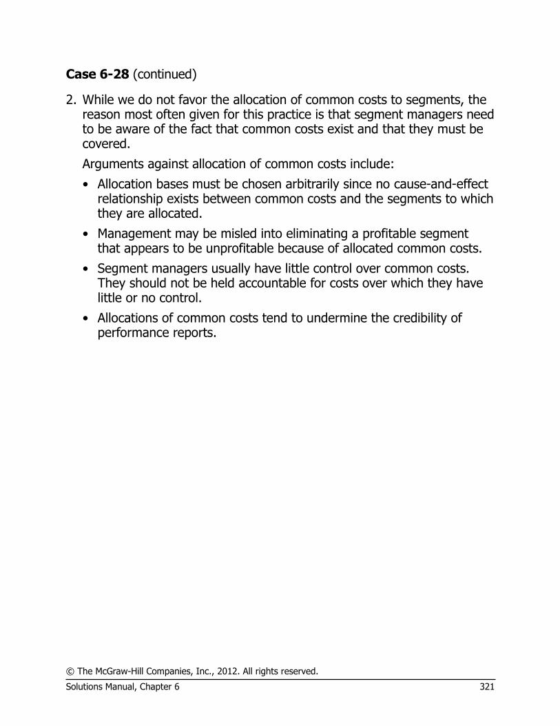
© The McGraw-Hill Companies, Inc., 2012. All rights reserved.
Solutions Manual, Chapter 6 321
Case 6-28 (continued)
2. While we do not favor the allocation of common costs to segments, the reason most often given for this practice is that segment managers need to be aware of the fact that common costs exist and that they must be covered.
Arguments against allocation of common costs include:
• Allocation bases must be chosen arbitrarily since no cause-and-effect relationship exists between common costs and the segments to which they are allocated.
• Management may be misled into eliminating a profitable segment that appears to be unprofitable because of allocated common costs.
• Segment managers usually have little control over common costs. They should not be held accountable for costs over which they have little or no control.
• Allocations of common costs tend to undermine the credibility of performance reports.

© The McGraw-Hill Companies, Inc., 2012. All rights reserved. Solutions Manual, Chapter 7 323
Chapter 7 Activity-Based Costing: A Tool to Aid Decision Making
Solutions to Questions
7-1 Activity-based costing differs from traditional costing systems in a number of ways. In activity-based costing, nonmanufacturing as well as manufacturing costs may be assigned to products. And, some manufacturing costs—including the costs of idle capacity—may be excluded from product costs. An activity-based costing system typically includes a number of activity cost pools, each of which has its unique measure of activity. These measures of activity often differ from the allocation bases used in traditional costing systems.
7-2 When direct labor is used as an allocation base for overhead, it is implicitly assumed that overhead cost is directly proportional to direct labor. When cost systems were originally developed in the 1800s, this assumption may have been reasonably accurate. However, direct labor has declined in importance over the years while overhead has been increasing. This suggests that there is no longer a direct link between the level of direct labor and overhead. Indeed, when a company automates, direct labor is replaced by machines; a decrease in direct labor is accompanied by an increase in overhead. This violates the assumption that overhead cost is directly proportional to direct labor. Overhead cost appears to be driven by factors such as product diversity and complexity as well as by volume, for which direct labor has served as a convenient measure.
7-3 Top managers provide leadership that is needed to properly motivate all employees to embrace the need to implement ABC. Top managers also have the authority to link ABC data to the employee evaluation and reward system. Cross-functional employees are also important because they possess intimate knowledge of operations that is needed to design an effective
ABC system. Tapping the knowledge of cross-functional employees also lessens their resistance to ABC because they feel included in the implementation process.
7-4 Unit-level activities are performed for each unit that is produced. Batch-level activities are performed for each batch regardless of how many units are in the batch. Product-level activities must be carried out to support a product regardless of how many batches are run or units produced. Customer-level activities must be carried out to support customers regardless of what products or services they buy. Organization-sustaining activities are carried out regardless of the company’s precise product mix or mix of customers.
7-5 Organization-sustaining costs, customer-level costs, and the costs of idle capacity should not be assigned to products. These costs represent resources that are not consumed by the products.
7-6 In activity-based costing, costs must first be allocated to activity cost pools and then they are allocated from the activity cost pools to products, customers, and other cost objects.
7-7 Because people are often involved in more than one activity, some way must be found to estimate how much time they spend in each activity. The most practical approach is often to ask employees how they spend their time. It is also possible to ask people to keep records of how they spend their time or observe them as they perform their tasks, but both of these alternatives are costly and it is not obvious that the data would be any better. People who know they are being observed may change how they behave.
© The McGraw-Hill Companies, Inc., 2012. All rights reserved. 324 Managerial Accounting, 14th Edition
7-8 In traditional cost systems, product-level costs are indiscriminately spread across all products using direct labor-hours or some other allocation base related to volume. As a consequence, high-volume products are assigned the bulk of such costs. If a product is responsible for 40% of the direct labor in a factory, it will be assigned 40% of the manufacturing overhead cost in the factory—including 40% of the product-level costs of low-volume products. In an activity-based costing system, batch-level and product-level costs are assigned more appropriately. This results in shifting product-level costs back to the products that cause them and away from the high-volume products. (A similar effect will be observed with batch-level costs if high-volume products are produced in larger batches than low-volume products.)
7-9 Activity rates tell managers the average cost of resources consumed to carry out a particular activity such as processing purchase orders. An activity whose average cost is high may be a good candidate for process improvements. Benchmarking can be used to identify which activities have unusually large costs. If some other organization is able to carry out the activity at a significantly lower cost, it is reasonable to suppose that improvement may be possible.
7-10 The activity-based costing approach described in the chapter is probably unacceptable for external financial reports for two reasons. First, activity-based product costs, as described in this chapter, exclude some manufacturing costs and include some nonmanufacturing costs. Second, the first-stage allocations are based on interviews rather than verifiable, objective data.
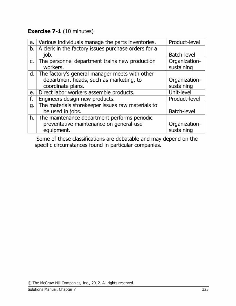
© The McGraw-Hill Companies, Inc., 2012. All rights reserved. Solutions Manual, Chapter 7 325
Exercise 7-1 (10 minutes)
a. Various individuals manage the parts inventories. Product-level b. A clerk in the factory issues purchase orders for a
job. Batch-level c. The personnel department trains new production
workers. Organization-sustaining
d. The factory’s general manager meets with other department heads, such as marketing, to coordinate plans.
Organization-sustaining
e. Direct labor workers assemble products. Unit-level f. Engineers design new products. Product-level g. The materials storekeeper issues raw materials to
be used in jobs. Batch-level h. The maintenance department performs periodic
preventative maintenance on general-use equipment.
Organization-sustaining
Some of these classifications are debatable and may depend on the specific circumstances found in particular companies.
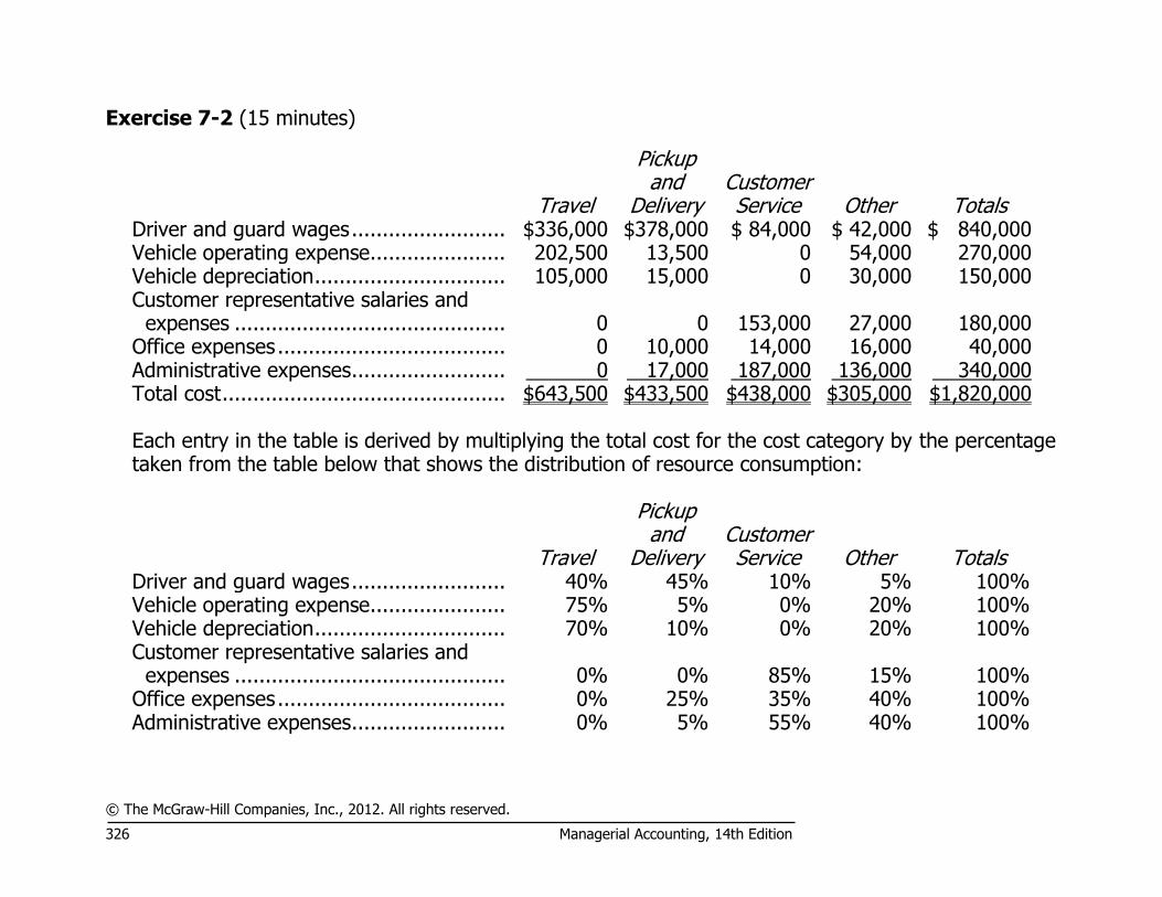
© The McGraw-Hill Companies, Inc., 2012. All rights reserved. 326 Managerial Accounting, 14th Edition
Exercise 7-2 (15 minutes)
Travel
Pickup and
Delivery Customer Service Other Totals
Driver and guard wages ......................... $336,000 $378,000 $ 84,000 $ 42,000 $ 840,000 Vehicle operating expense ...................... 202,500 13,500 0 54,000 270,000 Vehicle depreciation ............................... 105,000 15,000 0 30,000 150,000 Customer representative salaries and
expenses ............................................ 0 0 153,000 27,000 180,000 Office expenses ..................................... 0 10,000 14,000 16,000 40,000 Administrative expenses ......................... 0 17,000 187,000 136,000 340,000 Total cost .............................................. $643,500 $433,500 $438,000 $305,000 $1,820,000
Each entry in the table is derived by multiplying the total cost for the cost category by the percentage
taken from the table below that shows the distribution of resource consumption:
Travel
Pickup and
Delivery Customer Service Other Totals
Driver and guard wages ......................... 40% 45% 10% 5% 100% Vehicle operating expense ...................... 75% 5% 0% 20% 100% Vehicle depreciation ............................... 70% 10% 0% 20% 100% Customer representative salaries and
expenses ............................................ 0% 0% 85% 15% 100% Office expenses ..................................... 0% 25% 35% 40% 100% Administrative expenses ......................... 0% 5% 55% 40% 100%

© The McGraw-Hill Companies, Inc., 2012. All rights reserved. Solutions Manual, Chapter 7 327
Exercise 7-3 (10 minutes)
Activity Cost Pool
Estimated Overhead
Cost Expected Activity Activity Rate Caring for lawn $77,400 180,000 square feet of lawn $0.43 per square foot of lawn Caring for garden beds–
low maintenance $30,000 24,000 square feet of low
maintenance beds $1.25 per square foot of low
maintenance beds Caring for garden beds–
high maintenance $57,600 18,000 square feet of high
maintenance beds $3.20 per square foot of high
maintenance beds Travel to jobs $4,200 15,000 miles $0.28 per mile Customer billing and service $8,700 30 customers $290 per customer
The activity rate for each activity cost pool is computed by dividing its estimated overhead cost by its expected activity.
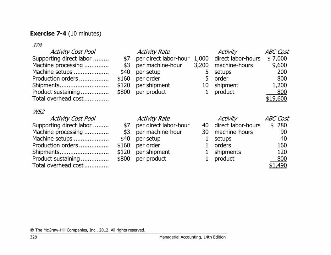
© The McGraw-Hill Companies, Inc., 2012. All rights reserved. 328 Managerial Accounting, 14th Edition
Exercise 7-4 (10 minutes)
J78 Activity Cost Pool Activity Rate Activity ABC Cost
Supporting direct labor ......... $7 per direct labor-hour 1,000 direct labor-hours $ 7,000 Machine processing .............. $3 per machine-hour 3,200 machine-hours 9,600 Machine setups .................... $40 per setup 5 setups 200 Production orders ................. $160 per order 5 order 800 Shipments ............................ $120 per shipment 10 shipment 1,200 Product sustaining ................ $800 per product 1 product 800 Total overhead cost .............. $19,600 W52
Activity Cost Pool Activity Rate Activity ABC Cost Supporting direct labor ......... $7 per direct labor-hour 40 direct labor-hours $ 280 Machine processing .............. $3 per machine-hour 30 machine-hours 90 Machine setups .................... $40 per setup 1 setups 40 Production orders ................. $160 per order 1 orders 160 Shipments ............................ $120 per shipment 1 shipments 120 Product sustaining ................ $800 per product 1 product 800 Total overhead cost .............. $1,490
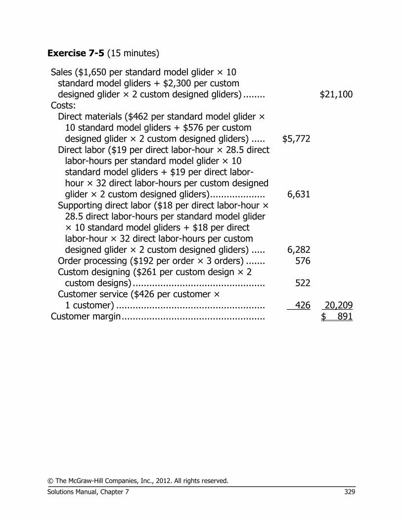
© The McGraw-Hill Companies, Inc., 2012. All rights reserved. Solutions Manual, Chapter 7 329
Exercise 7-5 (15 minutes)
Sales ($1,650 per standard model glider × 10 standard model gliders + $2,300 per custom designed glider × 2 custom designed gliders) ........ $21,100
Costs: Direct materials ($462 per standard model glider ×
10 standard model gliders + $576 per custom designed glider × 2 custom designed gliders) ..... $5,772
Direct labor ($19 per direct labor-hour × 28.5 direct labor-hours per standard model glider × 10 standard model gliders + $19 per direct labor-hour × 32 direct labor-hours per custom designed glider × 2 custom designed gliders) .................... 6,631
Supporting direct labor ($18 per direct labor-hour × 28.5 direct labor-hours per standard model glider × 10 standard model gliders + $18 per direct labor-hour × 32 direct labor-hours per custom designed glider × 2 custom designed gliders) ..... 6,282
Order processing ($192 per order × 3 orders) ....... 576 Custom designing ($261 per custom design × 2
custom designs) ................................................ 522 Customer service ($426 per customer ×
1 customer) ...................................................... 426 20,209 Customer margin .................................................... $ 891
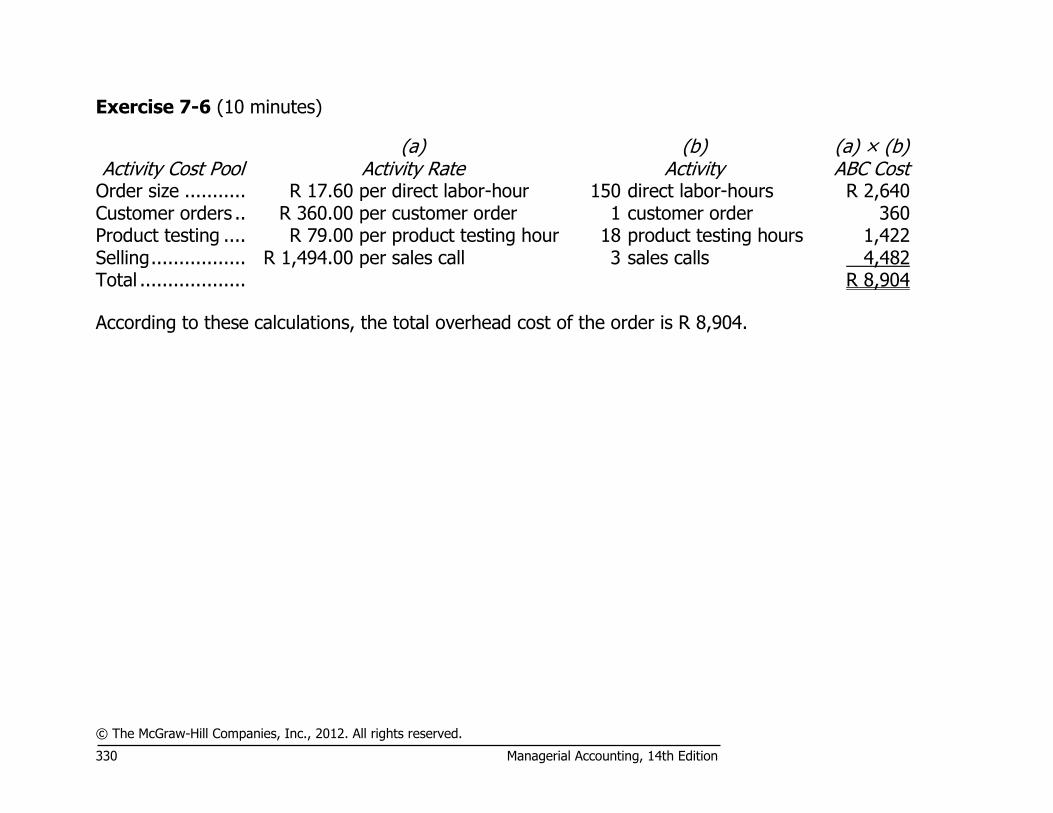
© The McGraw-Hill Companies, Inc., 2012. All rights reserved. 330 Managerial Accounting, 14th Edition
Exercise 7-6 (10 minutes)
Activity Cost Pool (a)
Activity Rate (b)
Activity (a) × (b) ABC Cost
Order size ........... R 17.60 per direct labor-hour 150 direct labor-hours R 2,640 Customer orders .. R 360.00 per customer order 1 customer order 360 Product testing .... R 79.00 per product testing hour 18 product testing hours 1,422 Selling ................. R 1,494.00 per sales call 3 sales calls 4,482 Total ................... R 8,904 According to these calculations, the total overhead cost of the order is R 8,904.

© The McGraw-Hill Companies, Inc., 2012. All rights reserved. Solutions Manual, Chapter 7 331
Exercise 7-7 (10 minutes)
Teller wages ............................... $150,000 Assistant branch manager salary .. $70,000 Branch manager salary ................ $85,000
Distribution of Resource Consumption Across Activities
Opening Accounts
Processing Deposits and Withdrawals
Processing Other
Customer Transactions
Other Activities Totals
Teller wages ............................... 0% 75% 15% 10% 100% Assistant branch manager salary .. 10% 15% 25% 50% 100% Branch manager salary ................ 0% 0% 20% 80% 100%
Opening Accounts
Processing Deposits and Withdrawals
Processing Other
Customer Transactions
Other Activities Totals
Teller wages ................................ $ 0 $112,500 $22,500 $ 15,000 $150,000 Assistant branch manager salary ... 7,000 10,500 17,500 35,000 70,000 Branch manager salary ................. 0 0 17,000 68,000 85,000 Total cost .................................... $7,000 $123,000 $57,000 $118,000 $305,000 Teller wages are $150,000 and 75% of the tellers’ time is spent processing deposits and withdrawals: $150,000 × 75% = $112,500 Other entries in the table are similarly determined.

© The McGraw-Hill Companies, Inc., 2012. All rights reserved. 332 Managerial Accounting, 14th Edition
Exercise 7-8 (20 minutes)
1. Computation of activity rates:
Activity Cost Pools (a)
Total Cost (b)
Total Activity (a) ÷ (b)
Activity Rate Opening accounts ................ $7,000 200 accounts
opened $35.00 per account
opened Processing deposits and
withdrawals ..................... $123,000 50,000 deposits and
withdrawals $2.46 per deposit or
withdrawal Processing other customer
transactions ..................... $57,000 1,000 other customer
transactions $57.00 per other customer
transaction 2. The cost of opening an account at the Avon branch is much higher than at the lowest cost branch
($35.00 versus $24.35). On the other hand, the cost of processing deposits and withdrawals is lower than at the lowest cost branch ($2.46 versus $2.72). And the cost of processing other customer transactions is somewhat higher at the Avon branch ($57.00 versus $48.90). The other branches may have something to learn from Avon concerning processing deposits and withdrawals and Avon may benefit from learning about how some of the other branches open accounts and process other transactions. It may be particularly instructive to compare the details of the activity rates. For example, is the cost of opening accounts at Avon apparently high because of the involvement of the assistant branch manager in this activity? Perhaps tellers open new accounts at other branches.
The apparent differences in the costs of the activities at the various branches could be due to inaccuracies in employees’ reports of the amount of time they devote to the activities. The differences in costs may also reflect different strategies. For example, the Avon branch may purposely spend more time with new customers to win their loyalty. The higher cost of opening new accounts at the Avon branch may be justified by future benefits of having more satisfied customers. Nevertheless, comparative studies of the costs of activities may provide a useful starting point for identifying best practices within a company and where improvements can be made.

© The McGraw-Hill Companies, Inc., 2012. All rights reserved. Solutions Manual, Chapter 7 333
Exercise 7-9 (30 minutes)
1. Total revenue received:
City
General County General
Cost of goods sold to the hospital (a) ........... $30,000 $30,000 Markup percentage ..................................... × 5% × 5% Markup in dollars (b) ................................... $1,500 $1,500 Revenue received from hospitals (a) + (b) .... $31,500 $31,500
2. Activity Rates:
Activity Cost Pool
(a) Estimated Overhead
Cost (b)
Expected Activity (a) ÷ (b)
Activity rate Customer deliveries ............ $400,000 5,000 deliveries $80.00 per delivery Manual order processing ..... $300,000 4,000 orders $75.00 per manual order Electronic order processing . $200,000 12,500 orders $16.00 per electronic order Line item picking ................ $500,000 400,000 line items $1.25 per line item picked

© The McGraw-Hill Companies, Inc., 2012. All rights reserved. 334 Managerial Accounting, 14th Edition
Exercise 7-9 (continued)
3. Activity costs are assigned to the two hospitals as follows: City General:
Activity Cost Pool
(a) Activity Rate
(b) Activity
(a) × (b) ABC Cost
Customer deliveries ............ $80.00 per delivery 10 deliveries $ 800 Manual order processing ..... $75.00 per order 0 orders 0 Electronic order processing . $16.00 per order 10 orders 160 Line item picking ................ $1.25 per line item 100 line items 125 Total activity costs .............. $1,085 County General:
Activity Cost Pool
(a) Activity Rate
(b) Activity
(a) × (b) ABC Cost
Customer deliveries ............ $80.00 per delivery 20 deliveries $1,600 Manual order processing ..... $75.00 per order 40 orders 3,000 Electronic order processing . $16.00 per order 0 orders 0 Line item picking ................ $1.25 per line item 260 line items 325 Total activity costs .............. $4,925
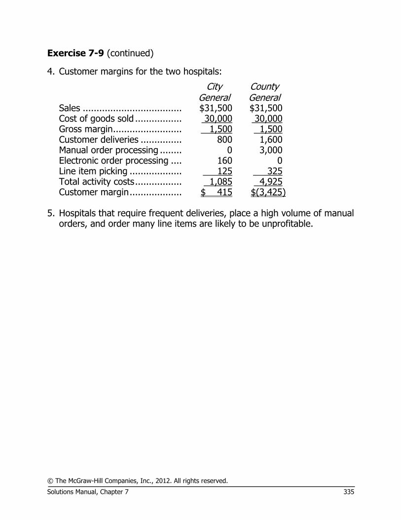
© The McGraw-Hill Companies, Inc., 2012. All rights reserved. Solutions Manual, Chapter 7 335
Exercise 7-9 (continued)
4. Customer margins for the two hospitals:
City General
County General
Sales .................................... $31,500 $31,500 Cost of goods sold ................. 30,000 30,000 Gross margin ......................... 1,500 1,500 Customer deliveries ............... 800 1,600 Manual order processing ........ 0 3,000 Electronic order processing .... 160 0 Line item picking ................... 125 325 Total activity costs ................. 1,085 4,925 Customer margin ................... $ 415 $(3,425)
5. Hospitals that require frequent deliveries, place a high volume of manual
orders, and order many line items are likely to be unprofitable.
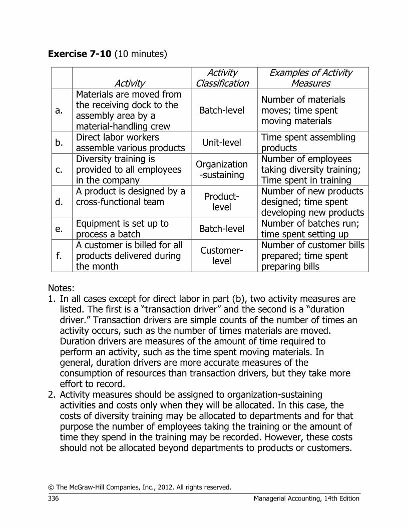
© The McGraw-Hill Companies, Inc., 2012. All rights reserved. 336 Managerial Accounting, 14th Edition
Exercise 7-10 (10 minutes)
Activity Activity
Classification Examples of Activity
Measures
a. Materials are moved from the receiving dock to the assembly area by a material-handling crew
Batch-level Number of materials moves; time spent moving materials
b. Direct labor workers assemble various products Unit-level Time spent assembling
products
c. Diversity training is provided to all employees in the company
Organization-sustaining
Number of employees taking diversity training; Time spent in training
d. A product is designed by a cross-functional team Product-
level Number of new products designed; time spent developing new products
e. Equipment is set up to process a batch Batch-level Number of batches run;
time spent setting up
f. A customer is billed for all products delivered during the month
Customer-level
Number of customer bills prepared; time spent preparing bills
Notes: 1. In all cases except for direct labor in part (b), two activity measures are
listed. The first is a “transaction driver” and the second is a “duration driver.” Transaction drivers are simple counts of the number of times an activity occurs, such as the number of times materials are moved. Duration drivers are measures of the amount of time required to perform an activity, such as the time spent moving materials. In general, duration drivers are more accurate measures of the consumption of resources than transaction drivers, but they take more effort to record.
2. Activity measures should be assigned to organization-sustaining activities and costs only when they will be allocated. In this case, the costs of diversity training may be allocated to departments and for that purpose the number of employees taking the training or the amount of time they spend in the training may be recorded. However, these costs should not be allocated beyond departments to products or customers.
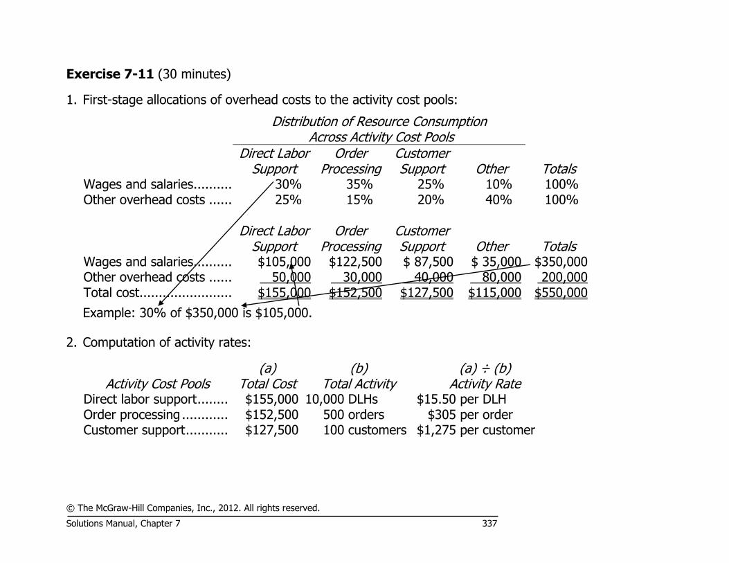
© The McGraw-Hill Companies, Inc., 2012. All rights reserved. Solutions Manual, Chapter 7 337
Exercise 7-11 (30 minutes)
1. First-stage allocations of overhead costs to the activity cost pools:
Distribution of Resource Consumption
Across Activity Cost Pools
Direct Labor
Support Order
Processing Customer Support Other Totals
Wages and salaries .......... 30% 35% 25% 10% 100% Other overhead costs ...... 25% 15% 20% 40% 100%
Direct Labor
Support Order
Processing Customer Support Other Totals
Wages and salaries .......... $105,000 $122,500 $ 87,500 $ 35,000 $350,000 Other overhead costs ...... 50,000 30,000 40,000 80,000 200,000 Total cost ........................ $155,000 $152,500 $127,500 $115,000 $550,000
Example: 30% of $350,000 is $105,000. 2. Computation of activity rates:
Activity Cost Pools (a)
Total Cost (b)
Total Activity (a) ÷ (b)
Activity Rate Direct labor support ........ $155,000 10,000 DLHs $15.50 per DLH Order processing ............ $152,500 500 orders $305 per order Customer support ........... $127,500 100 customers $1,275 per customer

© The McGraw-Hill Companies, Inc., 2012. All rights reserved. 338 Managerial Accounting, 14th Edition
Exercise 7-11 (continued)
3. Computation of the overhead costs for the Indus Telecom order:
Activity Cost Pool (a)
Activity Rate (b)
Activity (a) × (b) ABC Cost
Direct labor support ............. $15.50 per DLH 50 DLHs* $ 775
Order processing .. $305 per order 1 orders 305 Customer support . $1,275 per customer 1 customer 1,275 Total .................... $2,355
*0.5 DLH per unit × 100 units = 50 DLHs 4. The customer margin for Indus Telecom is computed as follows:
Customer Margin—ABC Analysis Sales (100 units × $295 per unit) ................. $29,500 Costs: Direct materials ($264 per unit × 100 units) . $26,400 Direct labor ($25 per DLH × 0.5 DLH per
unit × 100 units) ...................................... 1,250 Direct labor support overhead (see part 3
above) ..................................................... 775 Order processing overhead (see part 3
above) ..................................................... 305 Customer support overhead (see part 3
above) ..................................................... 1,275 30,005 Customer margin ........................................... $( 505)
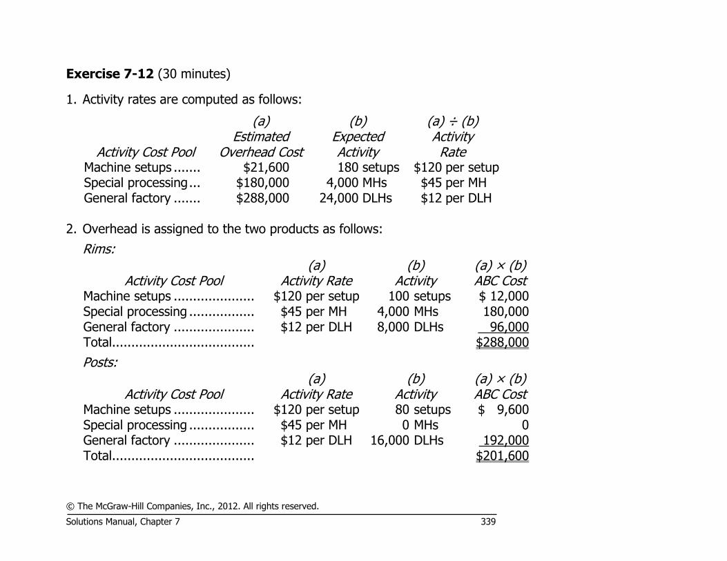
© The McGraw-Hill Companies, Inc., 2012. All rights reserved. Solutions Manual, Chapter 7 339
Exercise 7-12 (30 minutes)
1. Activity rates are computed as follows:
Activity Cost Pool
(a) Estimated
Overhead Cost
(b) Expected Activity
(a) ÷ (b) Activity Rate
Machine setups ....... $21,600 180 setups $120 per setup Special processing ... $180,000 4,000 MHs $45 per MH General factory ....... $288,000 24,000 DLHs $12 per DLH
2. Overhead is assigned to the two products as follows:
Rims:
Activity Cost Pool (a)
Activity Rate (b)
Activity (a) × (b) ABC Cost
Machine setups ..................... $120 per setup 100 setups $ 12,000 Special processing ................. $45 per MH 4,000 MHs 180,000 General factory ..................... $12 per DLH 8,000 DLHs 96,000 Total ..................................... $288,000
Posts:
Activity Cost Pool (a)
Activity Rate (b)
Activity (a) × (b) ABC Cost
Machine setups ..................... $120 per setup 80 setups $ 9,600 Special processing ................. $45 per MH 0 MHs 0 General factory ..................... $12 per DLH 16,000 DLHs 192,000 Total ..................................... $201,600
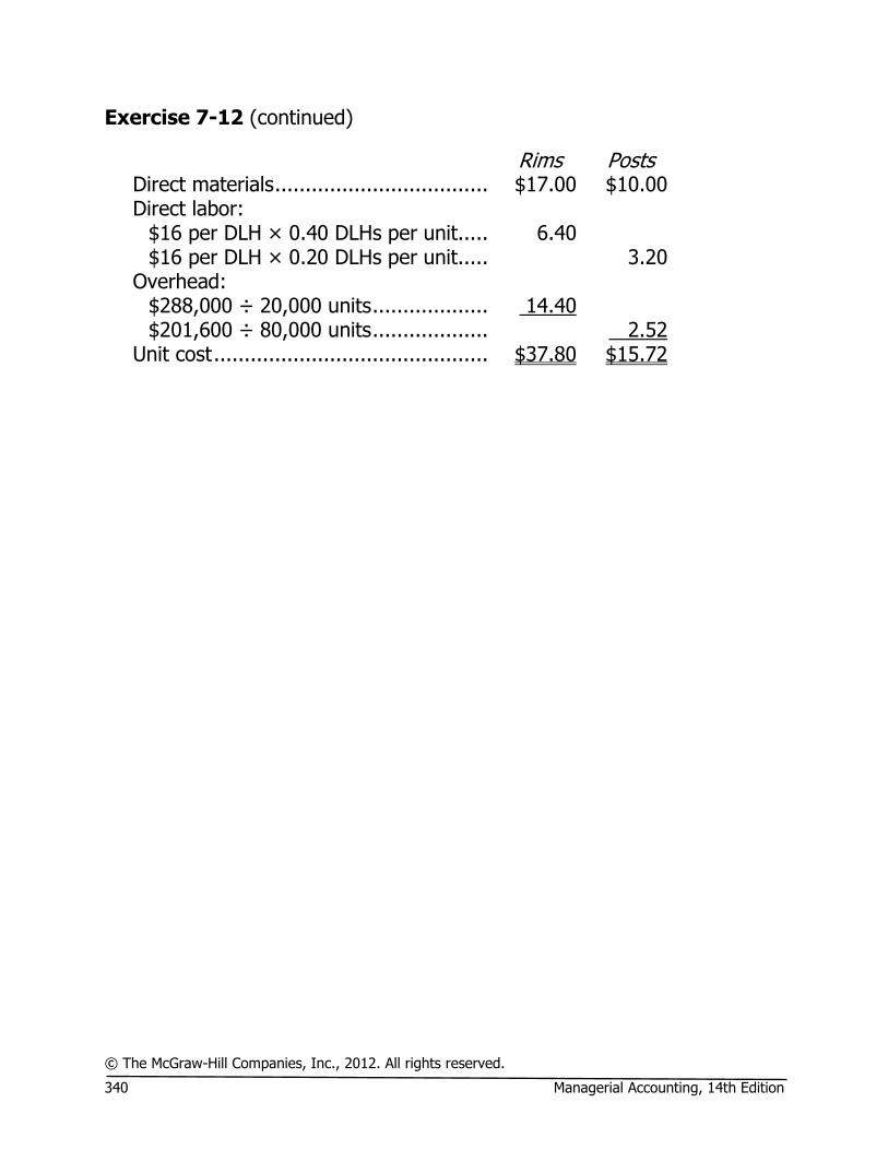
© The McGraw-Hill Companies, Inc., 2012. All rights reserved. 340 Managerial Accounting, 14th Edition
Exercise 7-12 (continued)
Rims Posts Direct materials ................................... $17.00 $10.00 Direct labor:
$16 per DLH × 0.40 DLHs per unit..... 6.40 $16 per DLH × 0.20 DLHs per unit..... 3.20
Overhead: $288,000 ÷ 20,000 units ................... 14.40 $201,600 ÷ 80,000 units ................... 2.52
Unit cost ............................................. $37.80 $15.72
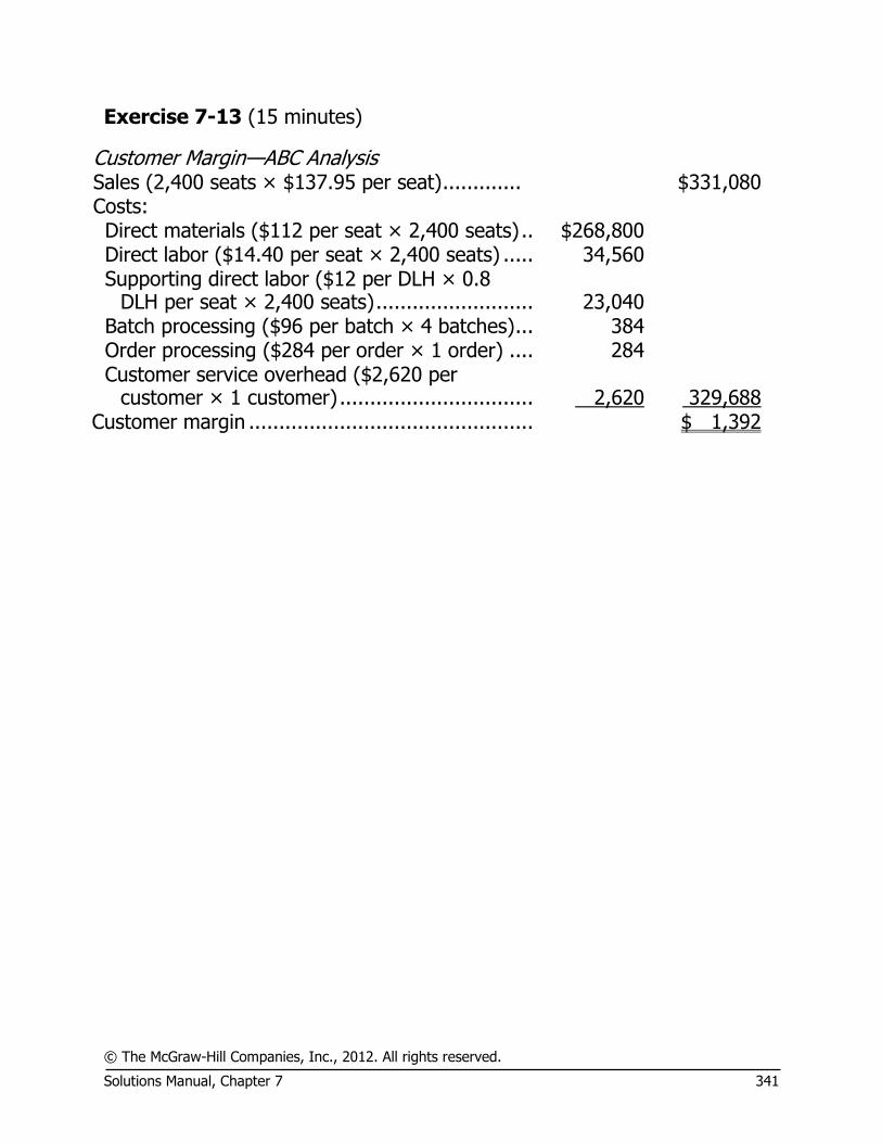
© The McGraw-Hill Companies, Inc., 2012. All rights reserved. Solutions Manual, Chapter 7 341
Exercise 7-13 (15 minutes)
Customer Margin—ABC Analysis Sales (2,400 seats × $137.95 per seat) ............. $331,080 Costs: Direct materials ($112 per seat × 2,400 seats) .. $268,800 Direct labor ($14.40 per seat × 2,400 seats) ..... 34,560 Supporting direct labor ($12 per DLH × 0.8
DLH per seat × 2,400 seats) .......................... 23,040 Batch processing ($96 per batch × 4 batches) ... 384 Order processing ($284 per order × 1 order) .... 284 Customer service overhead ($2,620 per
customer × 1 customer) ................................ 2,620 329,688 Customer margin ............................................... $ 1,392
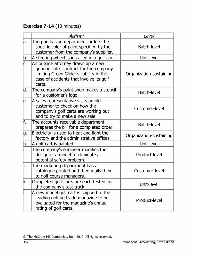
© The McGraw-Hill Companies, Inc., 2012. All rights reserved. 342 Managerial Accounting, 14th Edition
Exercise 7-14 (10 minutes)
Activity Level a. The purchasing department orders the
specific color of paint specified by the customer from the company’s supplier.
Batch-level
b. A steering wheel is installed in a golf cart. Unit-level c. An outside attorney draws up a new
generic sales contract for the company limiting Green Glider’s liability in the case of accidents that involve its golf carts.
Organization-sustaining
d. The company’s paint shop makes a stencil for a customer’s logo. Batch-level
e. A sales representative visits an old customer to check on how the company’s golf carts are working out and to try to make a new sale.
Customer-level
f. The accounts receivable department prepares the bill for a completed order. Batch-level
g. Electricity is used to heat and light the factory and the administrative offices. Organization-sustaining
h. A golf cart is painted. Unit-level i. The company’s engineer modifies the
design of a model to eliminate a potential safety problem.
Product-level
j. The marketing department has a catalogue printed and then mails them to golf course managers.
Customer-level
k. Completed golf carts are each tested on the company’s test track. Unit-level
l. A new model golf cart is shipped to the leading golfing trade magazine to be evaluated for the magazine’s annual rating of golf carts.
Product-level
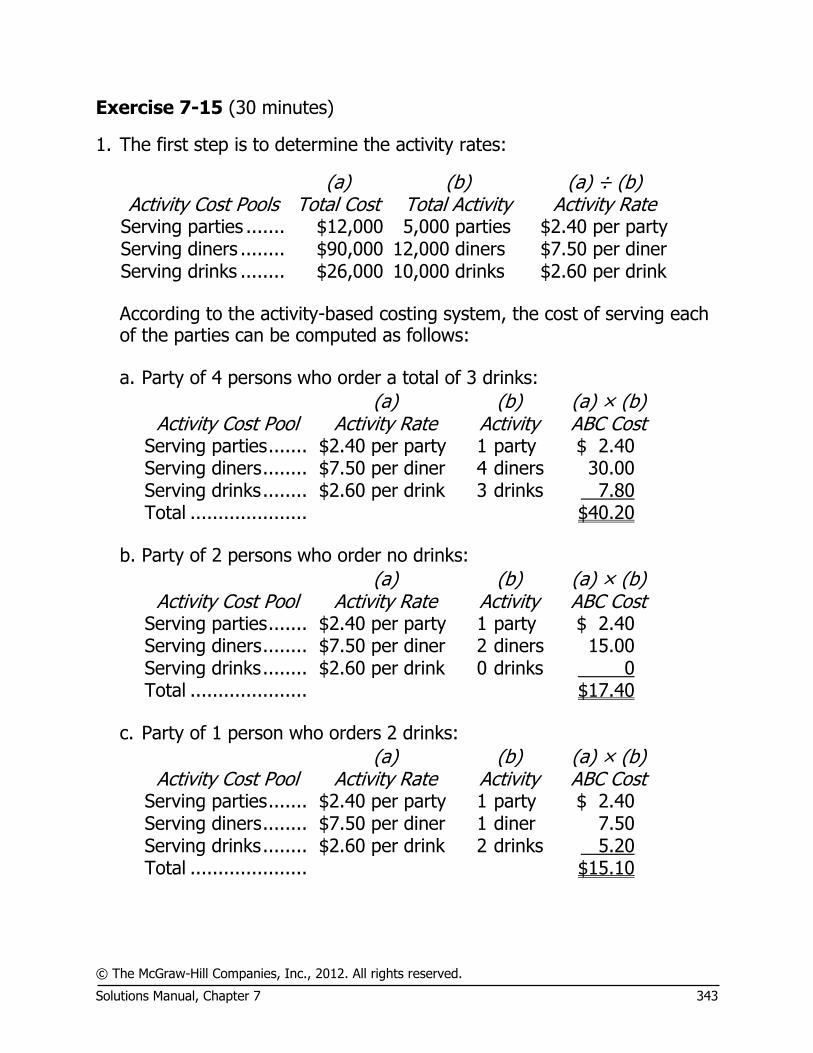
© The McGraw-Hill Companies, Inc., 2012. All rights reserved. Solutions Manual, Chapter 7 343
Exercise 7-15 (30 minutes)
1. The first step is to determine the activity rates:
Activity Cost Pools
(a) Total Cost
(b) Total Activity
(a) ÷ (b) Activity Rate
Serving parties ....... $12,000 5,000 parties $2.40 per party Serving diners ........ $90,000 12,000 diners $7.50 per diner Serving drinks ........ $26,000 10,000 drinks $2.60 per drink According to the activity-based costing system, the cost of serving each
of the parties can be computed as follows: a. Party of 4 persons who order a total of 3 drinks:
Activity Cost Pool
(a) Activity Rate
(b) Activity
(a) × (b) ABC Cost
Serving parties ....... $2.40 per party 1 party $ 2.40 Serving diners ........ $7.50 per diner 4 diners 30.00 Serving drinks ........ $2.60 per drink 3 drinks 7.80 Total ..................... $40.20 b. Party of 2 persons who order no drinks:
Activity Cost Pool
(a) Activity Rate
(b) Activity
(a) × (b) ABC Cost
Serving parties ....... $2.40 per party 1 party $ 2.40 Serving diners ........ $7.50 per diner 2 diners 15.00 Serving drinks ........ $2.60 per drink 0 drinks 0 Total ..................... $17.40 c. Party of 1 person who orders 2 drinks:
Activity Cost Pool
(a) Activity Rate
(b) Activity
(a) × (b) ABC Cost
Serving parties ....... $2.40 per party 1 party $ 2.40 Serving diners ........ $7.50 per diner 1 diner 7.50 Serving drinks ........ $2.60 per drink 2 drinks 5.20 Total ..................... $15.10

© The McGraw-Hill Companies, Inc., 2012. All rights reserved. 344 Managerial Accounting, 14th Edition
Exercise 7-15 (continued)
2. The average cost per diner for each party can be computed by dividing the total cost of the party by the number of diners in the party as follows:
a. $40.20 ÷ 4 diners = $10.05 per diner b. $17.40 ÷ 2 diners = $8.70 per diner c. $15.10 ÷ 1 diner = $15.10 per diner 3. The average cost per diner differs from party to party under the activity-
based costing system for two reasons. First, the $2.40 cost of serving a party does not depend on the number of diners in the party. Therefore, the average cost per diner of this activity decreases as the number of diners in the party increases. With only one diner, the cost is $2.40. With two diners, the average cost per diner is cut in half to $1.20. With six diners, the average cost per diner would be only $0.40. And so on. Second, the average cost per diner differs also because of the differences in the number of drinks ordered by the diners. If a party does not order any drinks, as was the case with the party of two, no costs of serving drinks are assigned to the party.
The average cost per diner under the ABC system differs from the overall average cost of $15 per diner for several reasons. First, the average cost of $15 per diner includes organization-sustaining costs that are excluded from the computations in the activity-based costing system. Second, the $15 per diner figure does not recognize differences in the diners’ demands on resources. It does not recognize that some diners order more drinks than others, nor does it recognize that there are some economies of scale in serving larger parties. (The batch-level costs of serving a party can be spread over more diners if the party is larger.)
We should note that the activity-based costing system itself does not recognize all of the differences in diners’ demands on resources. For example, the costs of preparing the various meals on the menu surely differ. It may or may not be worth the effort to build a more detailed activity-based costing system that would take into account such nuances.

© The McGraw-Hill Companies, Inc., 2012. All rights reserved. Solutions Manual, Chapter 7 345
Problem 7-16 (20 minutes)
1. The cost of serving the local commercial market according to the ABC model can be determined as follows:
Activity Cost Pool
(a) Activity Rate
(b) Activity
(a) × (b) ABC Cost
Animation concept ........ $6,000 per proposal 20 proposals $120,000 Animation production .... $7,700 per minute of animation 12 minutes 92,400 Contract administration . $6,600 per contract 8 contracts 52,800 $265,200 2. The margin earned serving the local commercial market is negative, as shown below:
Profitability Analysis Sales ................................................... $240,000 Costs: Animation concept .............................. $120,000 Animation production .......................... 92,400 Contract administration ....................... 52,800 265,200
Margin ................................................. $(25,200) 3. It appears that the local commercial market is losing money and the company would be better off
dropping this market segment. However, not all of the costs included above may be avoidable. If more than $25,200 of the total costs of $265,200 is not avoidable, then the company really isn’t losing money on the local commercial market and the segment should not be dropped. These issues will be discussed in more depth in later chapters.
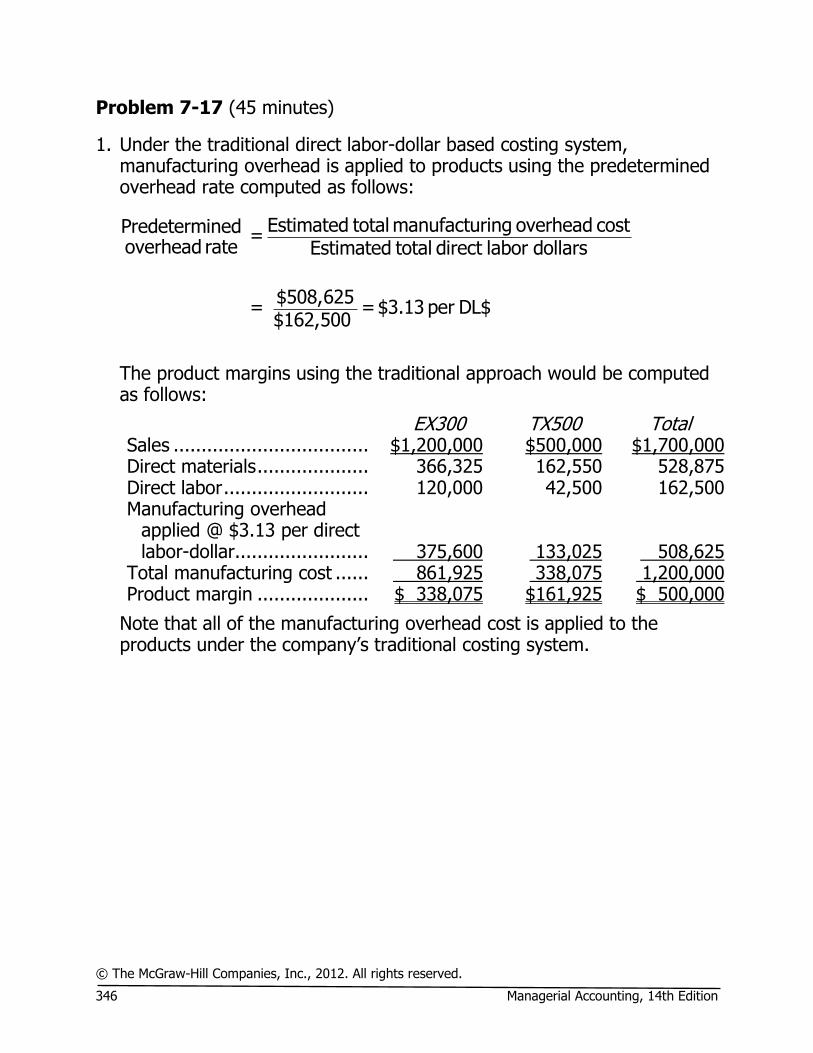
© The McGraw-Hill Companies, Inc., 2012. All rights reserved. 346 Managerial Accounting, 14th Edition
Problem 7-17 (45 minutes)
1. Under the traditional direct labor-dollar based costing system, manufacturing overhead is applied to products using the predetermined overhead rate computed as follows:
Estimated total manufacturing overhead costPredetermined = overhead rate Estimated total direct labor dollars
$508,625 = = $3.13 per DL$$162,500
The product margins using the traditional approach would be computed
as follows:
EX300 TX500 Total Sales ................................... $1,200,000 $500,000 $1,700,000 Direct materials .................... 366,325 162,550 528,875 Direct labor .......................... 120,000 42,500 162,500 Manufacturing overhead
applied @ $3.13 per direct labor-dollar........................ 375,600 133,025 508,625
Total manufacturing cost ...... 861,925 338,075 1,200,000 Product margin .................... $ 338,075 $161,925 $ 500,000
Note that all of the manufacturing overhead cost is applied to the products under the company’s traditional costing system.
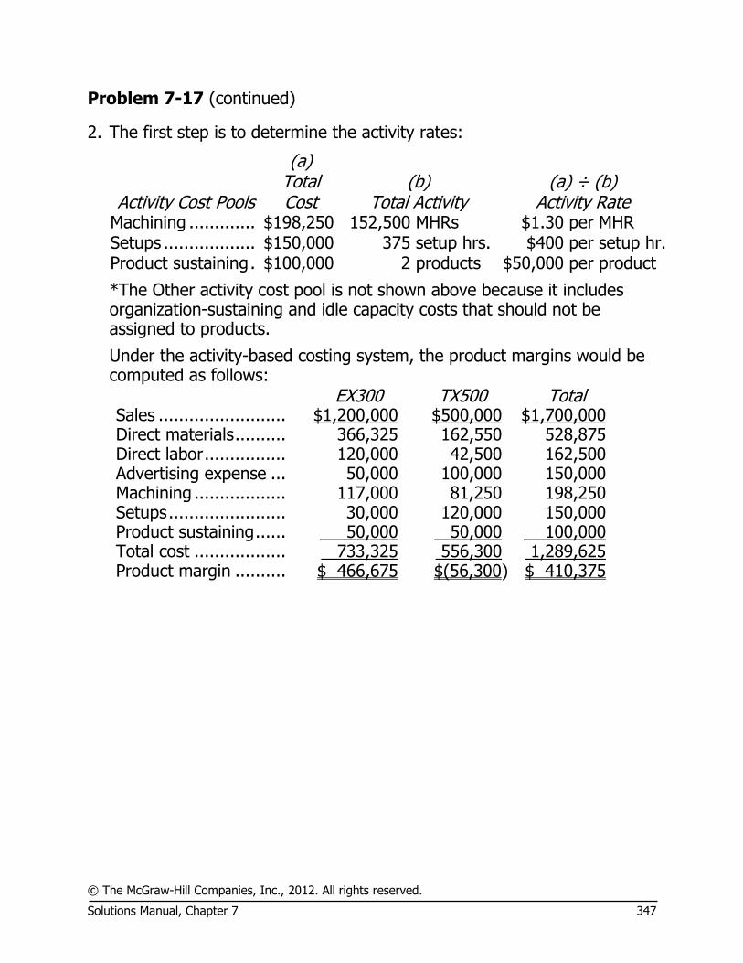
© The McGraw-Hill Companies, Inc., 2012. All rights reserved. Solutions Manual, Chapter 7 347
Problem 7-17 (continued)
2. The first step is to determine the activity rates:
Activity Cost Pools
(a) Total Cost
(b) Total Activity
(a) ÷ (b) Activity Rate
Machining ............. $198,250 152,500 MHRs $1.30 per MHR Setups .................. $150,000 375 setup hrs. $400 per setup hr. Product sustaining . $100,000 2 products $50,000 per product
*The Other activity cost pool is not shown above because it includes organization-sustaining and idle capacity costs that should not be assigned to products.
Under the activity-based costing system, the product margins would be computed as follows:
EX300 TX500 Total Sales ......................... $1,200,000 $500,000 $1,700,000 Direct materials .......... 366,325 162,550 528,875 Direct labor ................ 120,000 42,500 162,500 Advertising expense ... 50,000 100,000 150,000 Machining .................. 117,000 81,250 198,250 Setups ....................... 30,000 120,000 150,000 Product sustaining ...... 50,000 50,000 100,000 Total cost .................. 733,325 556,300 1,289,625 Product margin .......... $ 466,675 $(56,300) $ 410,375

© The McGraw-Hill Companies, Inc., 2012. All rights reserved. 348 Managerial Accounting, 14th Edition
Problem 7-17 (continued)
3. The quantitative comparison is as follows:
EX300 TX500 Total
Traditional Cost System (a)
Amount (a) ÷ (c)
% (b)
Amount (b) ÷ (c)
% (c)
Amount Direct materials ................................. $366,325 69.3% $162,550 30.7% $ 528,875 Direct labor ....................................... 120,000 73.8% 42,500 26.2% 162,500 Manufacturing overhead .................... 375,600 73.8% 133,025 26.2% 508,625 Total cost assigned to products .......... $861,925 $338,075 1,200,000 Selling and administrative .................. 550,000 Total cost .......................................... $1,750,000 Activity-Based Costing System Direct costs:
Direct materials .............................. $366,325 69.3% $162,550 30.7% $ 528,875 Direct labor .................................... 120,000 73.8% 42,500 26.2% 162,500 Advertising expense ........................ 50,000 33.3% 100,000 66.7% 150,000
Indirect costs: Machining ....................................... 117,000 59.0% 81,250 41.0% 198,250 Setups ............................................ 30,000 20.0% 120,000 80.0% 150,000 Product sustaining .......................... 50,000 50.0% 50,000 50.0% 100,000
Total cost assigned to products .......... $733,325 $556,300 1,289,625 Costs not assigned to products:
Selling and administrative ................ 400,000 Other ............................................. 60,375
Total cost .......................................... $1,750,000

© The McGraw-Hill Companies, Inc., 2012. All rights reserved. Solutions Manual, Chapter 7 349
Problem 7-17 (continued)
The traditional and activity-based cost assignments differ for three reasons. First, the traditional system assigns all $508,625 of manufacturing overhead to products. The ABC system assigns only $448,250 of manufacturing overhead to products. The ABC system does not assign the $60,375 of Other activity costs to products because they represent organization-sustaining costs. Second, the traditional system uses one unit-level activity measure, direct labor dollars, to assign 73.9% of all overhead to the EX300 product line and 26.1% of all overhead to the TX500 product line. The ABC system assigns 59.0% of Machining costs to the EX300 product line and 41.0% to the TX500 product line. The ABC system assigns 20.0% of Setup costs (a batch-level activity) to the EX300 product line and 80.0% to the TX500 product line. The ABC system assigns 50% of Product sustaining costs (a product-level activity) to each product line. Third, the traditional system does not trace any advertising expenses to the two products. The ABC system traces $50,000 of advertising to the EX300 and $100,000 of advertising to the TX500 product line.
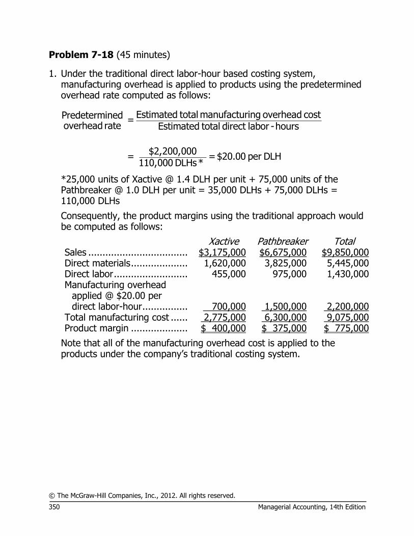
© The McGraw-Hill Companies, Inc., 2012. All rights reserved. 350 Managerial Accounting, 14th Edition
Problem 7-18 (45 minutes)
1. Under the traditional direct labor-hour based costing system, manufacturing overhead is applied to products using the predetermined overhead rate computed as follows:
Estimated total manufacturing overhead costPredetermined = overhead rate Estimated total direct labor -hours
$2,200,000 = = $20.00 per DLH110,000 DLHs*
*25,000 units of Xactive @ 1.4 DLH per unit + 75,000 units of the Pathbreaker @ 1.0 DLH per unit = 35,000 DLHs + 75,000 DLHs = 110,000 DLHs
Consequently, the product margins using the traditional approach would be computed as follows:
Xactive Pathbreaker Total Sales ................................... $3,175,000 $6,675,000 $9,850,000 Direct materials .................... 1,620,000 3,825,000 5,445,000 Direct labor .......................... 455,000 975,000 1,430,000 Manufacturing overhead
applied @ $20.00 per direct labor-hour ................ 700,000 1,500,000 2,200,000
Total manufacturing cost ...... 2,775,000 6,300,000 9,075,000 Product margin .................... $ 400,000 $ 375,000 $ 775,000
Note that all of the manufacturing overhead cost is applied to the products under the company’s traditional costing system.
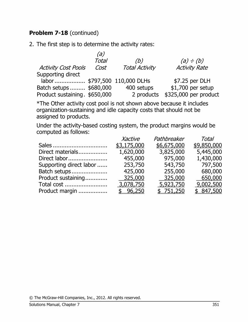
© The McGraw-Hill Companies, Inc., 2012. All rights reserved. Solutions Manual, Chapter 7 351
Problem 7-18 (continued)
2. The first step is to determine the activity rates:
Activity Cost Pools
(a) Total Cost
(b) Total Activity
(a) ÷ (b) Activity Rate
Supporting direct labor .................. $797,500 110,000 DLHs $7.25 per DLH
Batch setups ......... $680,000 400 setups $1,700 per setup Product sustaining . $650,000 2 products $325,000 per product
*The Other activity cost pool is not shown above because it includes organization-sustaining and idle capacity costs that should not be assigned to products.
Under the activity-based costing system, the product margins would be computed as follows:
Xactive Pathbreaker Total Sales ................................ $3,175,000 $6,675,000 $9,850,000 Direct materials ................. 1,620,000 3,825,000 5,445,000 Direct labor ....................... 455,000 975,000 1,430,000 Supporting direct labor ...... 253,750 543,750 797,500 Batch setups ..................... 425,000 255,000 680,000 Product sustaining ............. 325,000 325,000 650,000 Total cost ......................... 3,078,750 5,923,750 9,002,500 Product margin ................. $ 96,250 $ 751,250 $ 847,500

© The McGraw-Hill Companies, Inc., 2012. All rights reserved. 352 Managerial Accounting, 14th Edition
Problem 7-18 (continued)
3. The quantitative comparison is as follows:
Xactive Pathbreaker Total
Traditional Cost System (a)
Amount (a) ÷ (c)
% (b)
Amount (b) ÷ (c)
% (c)
Amount Direct materials ......................... $1,620,000 29.8% $3,825,000 70.2% $5,445,000 Direct labor ............................... 455,000 31.8% 975,000 68.2% 1,430,000 Manufacturing overhead ............ 700,000 31.8% 1,500,000 68.2% 2,200,000 Total cost assigned to products .. $2,775,000 $6,300,000 $9,075,000 Activity-Based Costing System Direct costs:
Direct materials ...................... $1,620,000 29.8% $3,825,000 70.2% $5,445,000 Direct labor ............................ 455,000 31.8% 975,000 68.2% 1,430,000
Indirect costs: Supporting direct labor ............ 253,750 31.8% 543,750 68.2% 797,500 Batch setups ........................... 425,000 62.5% 255,000 37.5% 680,000 Product sustaining .................. 325,000 50.0% 325,000 50.0% 650,000
Total cost assigned to products .. $3,078,750 $5,923,750 9,002,500 Costs not assigned to products:
Other ..................................... 72,500 Total cost .................................. $9,075,000

© The McGraw-Hill Companies, Inc., 2012. All rights reserved. Solutions Manual, Chapter 7 353
Problem 7-18 (continued)
The traditional and activity-based cost assignments differ for two reasons. First, the traditional system assigns all $2,200,000 of manufacturing overhead to products. The ABC system assigns only $2,127,500 of manufacturing overhead to products. The ABC system does not assign the $72,500 of Other activity costs to products because they represent organization-sustaining and idle capacity costs. Second, the traditional system uses one unit-level activity measure, direct labor hours, to assign 31.8% of all overhead to the Xactive product line and 68.2% of all overhead to the Pathbreaker product line. The ABC system assigns 62.5% of Batch setup costs (a batch-level activity) to the Xactive product line and 37.5% to the Pathbreaker product line. The ABC system assigns 50% of Product sustaining costs (a product-level activity) to each product line.

© The McGraw-Hill Companies, Inc., 2012. All rights reserved. 354 Managerial Accounting, 14th Edition
Problem 7-19 (45 minutes)
1. The results of the first-stage allocation appear below:
Removing Asbestos
Estimating and Job Setup
Working on Nonroutine
Jobs Other Totals Wages and salaries ......... $ 80,000 $ 20,000 $ 70,000 $ 30,000 $ 200,000 Disposal fees ................... 420,000 0 180,000 0 600,000 Equipment depreciation ... 40,000 0 32,000 8,000 80,000 On-site supplies .............. 33,000 9,000 12,000 6,000 60,000 Office expenses ............... 19,000 76,000 57,000 38,000 190,000 Licensing and insurance ... 185,000 0 148,000 37,000 370,000 Total cost ....................... $777,000 $105,000 $499,000 $119,000 $1,500,000
According to the data in the problem, 40% of the wages and salaries cost of $200,000 is attributable to activities related to job size.
$200,000 × 40% = $80,000 Other entries in the table are determined in a similar manner. 2.
Activity Cost Pool (a)
Total Cost (b)
Total Activity (a) ÷ (b)
Activity Rate Removing
asbestos ........... $777,000 500 thousand square feet $1,554 per thousand square feet Estimating and job
setup ................ $105,000 200 jobs $525 per job Working on
nonroutine jobs . $499,000 25 nonroutine jobs $19,960 per nonroutine job

© The McGraw-Hill Companies, Inc., 2012. All rights reserved. Solutions Manual, Chapter 7 355
Problem 7-19 (continued)
3. The costs of each of the jobs can be computed as follows using the activity rates computed above: a. Routine two-thousand-square-foot job: Removing asbestos
($1,554 per thousand square feet × 2 thousand square feet) ..................... $3,108 Estimating and job setup ($525 per job × 1 job) .......................................... 525 Nonroutine job (not applicable) ................................................................... 0 Total cost of the job ................................................................................... $3,633 Average cost per thousand square feet ($3,633 ÷ 2 thousand square feet) ... $1,816.50 b. Routine four-thousand-square-foot job: Removing asbestos
($1,554 per thousand square feet × 4 thousand square feet) ..................... $6,216 Estimating and job setup ($525 per job × 1 job) .......................................... 525 Nonroutine job (not applicable) ................................................................... 0 Total cost of the job ................................................................................... $6,741 Cost per thousand square feet ($6,741 ÷ 4 thousand square feet) ................ $1,685.25 c. Nonroutine two-thousand-square-foot job: Removing asbestos
($1,554 per thousand square feet × 2 thousand square feet) ..................... $ 3,108 Estimating and job setup ($525 per job × 1 job) .......................................... 525 Nonroutine job ($19,960 per nonroutine job × 1 nonroutine job) .................. 19,960 Total cost of the job ................................................................................... $23,593 Cost per thousand square feet ($23,593 ÷ 2 thousand square feet) .............. $11,796.50
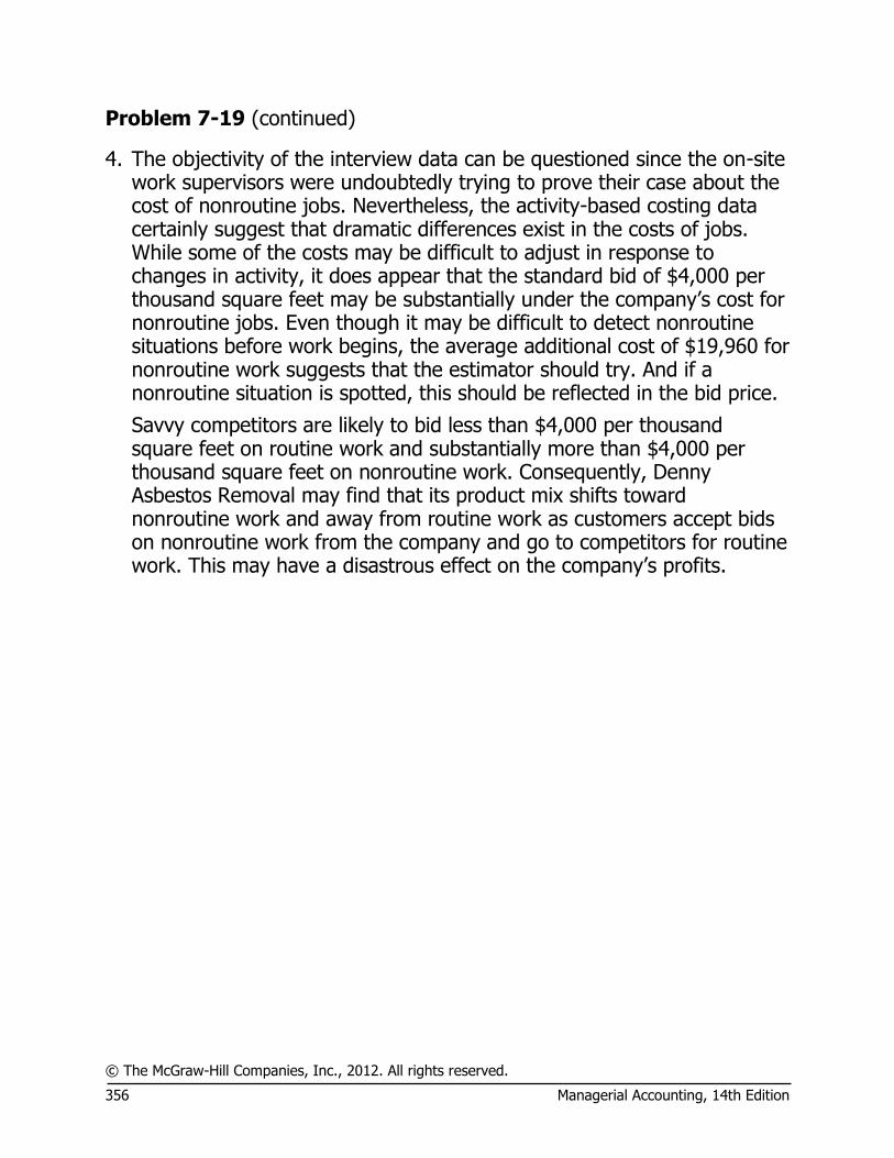
© The McGraw-Hill Companies, Inc., 2012. All rights reserved. 356 Managerial Accounting, 14th Edition
Problem 7-19 (continued)
4. The objectivity of the interview data can be questioned since the on-site work supervisors were undoubtedly trying to prove their case about the cost of nonroutine jobs. Nevertheless, the activity-based costing data certainly suggest that dramatic differences exist in the costs of jobs. While some of the costs may be difficult to adjust in response to changes in activity, it does appear that the standard bid of $4,000 per thousand square feet may be substantially under the company’s cost for nonroutine jobs. Even though it may be difficult to detect nonroutine situations before work begins, the average additional cost of $19,960 for nonroutine work suggests that the estimator should try. And if a nonroutine situation is spotted, this should be reflected in the bid price.
Savvy competitors are likely to bid less than $4,000 per thousand square feet on routine work and substantially more than $4,000 per thousand square feet on nonroutine work. Consequently, Denny Asbestos Removal may find that its product mix shifts toward nonroutine work and away from routine work as customers accept bids on nonroutine work from the company and go to competitors for routine work. This may have a disastrous effect on the company’s profits.

© The McGraw-Hill Companies, Inc., 2012. All rights reserved. Solutions Manual, Chapter 7 357
Problem 7-20 (45 minutes)
1. The first-stage allocation of costs to activity cost pools appears below:
Distribution of Resource Consumption
Across Activity Cost Pools
Cleaning Carpets
Travel to Jobs
Job Support Other Total
Wages ....................................... 75% 15% 0% 10% 100% Cleaning supplies ....................... 100% 0% 0% 0% 100% Cleaning equipment depreciation . 70% 0% 0% 30% 100% Vehicle expenses ........................ 0% 80% 0% 20% 100% Office expenses .......................... 0% 0% 60% 40% 100% President’s compensation ............ 0% 0% 30% 70% 100%
Cleaning Carpets
Travel to Jobs
Job Support Other Total
Wages ........................................ $105,000 $21,000 $ 0 $14,000 $140,000 Cleaning supplies ........................ 25,000 0 0 0 25,000 Cleaning equipment depreciation .. 7,000 0 0 3,000 10,000 Vehicle expenses ......................... 0 24,000 0 6,000 30,000 Office expenses ........................... 0 0 36,000 24,000 60,000 President’s compensation ............. 0 0 22,500 52,500 75,000 Total cost ................................... $137,000 $45,000 $58,500 $99,500 $340,000
75% of $140,000 = $105,000 Other entries in the table are determined in a similar manner.

© The McGraw-Hill Companies, Inc., 2012. All rights reserved. 358 Managerial Accounting, 14th Edition
Problem 7-20 (continued)
2. The activity rates are computed as follows:
Activity Cost Pool
(a) Total Cost
(b) Total Activity
(a) ÷ (b) Activity Rate
Cleaning carpets... $137,000 10,000 hundred square feet
$13.70 per hundred square feet
Travel to jobs ....... $45,000 50,000 miles $0.90 per mile Job support .......... $58,500 1,800 jobs $32.50 per job 3. The cost for the Lazy Bee Ranch job is computed as follows:
Activity Cost Pool (a)
Activity Rate (b)
Activity
(a) × (b) ABC Cost
Cleaning carpets ... $13.70 per hundred square feet
6 hundred square feet
$ 82.20
Travel to jobs ....... $0.90 per mile 52 miles 46.80 Job support .......... $32.50 per job 1 job 32.50 Total .................... $161.50 4. The product margin can be easily computed below by using the costs
calculated in part (3) above.
Sales ...................... $137.70 Costs:
Cleaning carpets ... $82.20 Travel to jobs ....... 46.80 Job support .......... 32.50 161.50
Product margin ....... $(23.80)

© The McGraw-Hill Companies, Inc., 2012. All rights reserved. Solutions Manual, Chapter 7 359
Problem 7-20 (continued)
5. Gore Range Carpet Cleaning appears to be losing money on the Lazy Bee Ranch job. However, caution is advised. Some of the costs may not be avoidable and hence would have been incurred even if the Lazy Bee Ranch job had not been accepted. An action analysis (discussed in Appendix 7A) is a more appropriate starting point for analysis than the simple report in part (4) above.
Nevertheless, there is a point at which travel costs eat up all of the profit from a job. With the company’s current policy of charging a flat fee for carpet cleaning irrespective of how far away the client is from the office, there clearly is some point at which jobs should be turned down. (What if a potential customer is located in Florida?)
6. The company should consider charging a fee for travel to outlying
customers based on the distance traveled and a flat fee per job. At present, close-in customers are in essence subsidizing service to outlying customers and large-volume customers are subsidizing service to low-volume customers. With fees for travel and for job support, the fee per hundred square feet can be dropped substantially. This may result in losing some low-volume jobs in outlying areas, but the lower fee per hundred square feet may result in substantially more business close to Eagle-Vail. (If the fee is low enough, the added business may not even have to come at the expense of competitors. Some customers may choose to clean their carpets more frequently if the price were more attractive.)

© The McGraw-Hill Companies, Inc., 2012. All rights reserved. 360 Managerial Accounting, 14th Edition
Appendix 7A ABC Action Analysis
Exercise 7A-1 (20 minutes)
Sales (80 clubs × $48 per club) ............................ $3,840.00 Green costs: Direct materials (80 clubs × $25.40 per club) ...... $2,032.00 2,032.00
Green margin ...................................................... 1,808.00 Yellow costs: Direct labor (80 clubs × 0.3 hour per club ×
$21.50 per hour) ............................................. 516.00 Indirect labor ..................................................... 90.00 Marketing expenses ........................................... 540.20 1,146.20
Yellow margin ...................................................... 661.80 Red costs: Factory equipment depreciation .......................... 106.40 Factory administration ........................................ 262.40 Selling and administrative wages and salaries ...... 436.00 Selling and administrative depreciation ................ 30.00 834.80
Red margin ......................................................... $ (173.00) While not required in the problem, the conventional ABC analysis would be:
Sales (80 clubs × $48 per club) ............................ $3,840.00 Costs:
Direct materials ................................................. $2,032.00 Direct labor ....................................................... 516.00 Volume related overhead ................................... 283.20 Batch processing overhead ................................ 53.00 Order processing overhead ................................ 118.80 Customer service overhead ................................ 1,010.00 4,013.00
Customer margin ................................................. $ (173.00)

© The McGraw-Hill Companies, Inc., 2012. All rights reserved. Solutions Manual, Appendix 7A 361
Exercise 7A-2 (30 minutes)
1. Order Size
Customer Orders
Product Testing Selling Total
Total activity for the order ........ 150 1 18 3
direct labor-hours
customer order
product testing hours
sales calls
Manufacturing overhead:
Indirect labor ........................ R 1,440 R 231 R 648 R 0 R 2,319 Factory depreciation .............. 1,050 0 324 0 1,374 Factory utilities ...................... 30 0 18 0 48 Factory administration ........... 0 46 432 36 514
Selling and administrative: Wages and salaries ............... 120 72 0 2,895 3,087 Depreciation ......................... 0 11 0 108 119 Taxes and insurance .............. 0 0 0 147 147 Selling expenses .................... 0 0 0 1,296 1,296
Total overhead cost ................. R 2,640 R 360 R 1,422 R 4,482 R 8,904
Example: R 9.60 per direct labor-hour × 150 direct labor-hours = R 1,440
According to these calculations, the overhead cost of the order was R 8,904. This agrees with the computations in Exercise 7-6.

© The McGraw-Hill Companies, Inc., 2012. All rights reserved. 362 Managerial Accounting, 14th Edition
Exercise 7A-2 (continued)
2. The table prepared in part (1) above allows two different perspectives on the overhead cost of the order. The column totals that appear in the last row of the table tell us the cost of the order in terms of the activities it required. The row totals that appear in the last column of the table tell us how much the order cost in terms of the overhead accounts in the underlying accounting system. Another way of saying this is that the column totals tell us what the costs were incurred for. The row totals tell us what the costs were incurred on. For example, you may spend money on a chocolate bar to satisfy your craving for chocolate. Both perspectives are important. To control costs, it is necessary both to know what the costs were incurred for and what actual costs would have to be adjusted (i.e., what the costs were incurred on).
The two different perspectives can be explicitly shown as follows:
What the overhead costs were spent on: Manufacturing overhead:
Indirect labor ................................ R 2,319 Factory depreciation ...................... 1,374 Factory utilities .............................. 48 Factory administration ................... 514
Selling and administrative: Wages and salaries ........................ 3,087 Depreciation .................................. 119 Taxes and insurance ...................... 147 Selling expenses ............................ 1,296
Total overhead cost .......................... R 8,904
What the overhead costs were incurred for: Order size ........................................ R 2,640 Customer orders .............................. 360 Product testing ................................ 1,422 Selling ............................................. 4,482 Total overhead cost .......................... R 8,904

© The McGraw-Hill Companies, Inc., 2012. All rights reserved. Solutions Manual, Appendix 7A 363
Exercise 7A-3 (30 minutes)
Supporting Direct Labor
Batch Processing
Order Processing
Customer Service Total
Total activity for the order ....................... 1,920 4 1 1
direct labor-
hours* batches order customer
Manufacturing overhead: Indirect labor ....................................... $ 3,456 $288 $ 18 $ 0 $ 3,762 Factory equipment depreciation ............ 14,112 13 0 0 14,125 Factory administration .......................... 4,032 28 28 268 4,356
Selling and administrative: Wages and salaries .............................. 960 52 153 1,864 3,029 Depreciation ........................................ 0 3 6 26 35 Marketing expenses ............................. 480 0 79 462 1,021
Total overhead cost ................................ $23,040 $384 $284 $2,620 $26,328
Example: $1.80 per direct labor-hour × 1,920 direct labor-hours = $3,456 *1,920 direct labor-hours = 0.8 direct labor-hour per seat × 2,400 seats
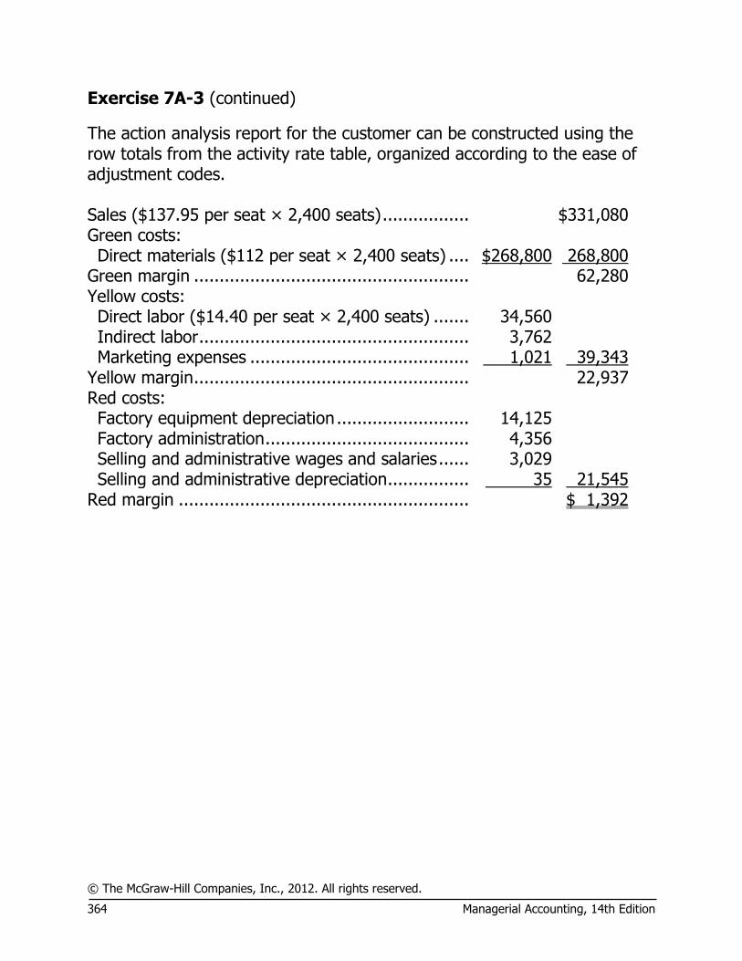
© The McGraw-Hill Companies, Inc., 2012. All rights reserved. 364 Managerial Accounting, 14th Edition
Exercise 7A-3 (continued)
The action analysis report for the customer can be constructed using the row totals from the activity rate table, organized according to the ease of adjustment codes. Sales ($137.95 per seat × 2,400 seats) ................. $331,080 Green costs: Direct materials ($112 per seat × 2,400 seats) .... $268,800 268,800
Green margin ...................................................... 62,280 Yellow costs: Direct labor ($14.40 per seat × 2,400 seats) ....... 34,560 Indirect labor ..................................................... 3,762 Marketing expenses ........................................... 1,021 39,343
Yellow margin ...................................................... 22,937 Red costs: Factory equipment depreciation .......................... 14,125 Factory administration ........................................ 4,356 Selling and administrative wages and salaries ...... 3,029 Selling and administrative depreciation ................ 35 21,545
Red margin ......................................................... $ 1,392

© The McGraw-Hill Companies, Inc., 2012. All rights reserved. Solutions Manual, Appendix 7A 365
Exercise 7A-4 (60 minutes)
1. First-stage allocations of overhead costs to the activity cost pools:
Distribution of Resource Consumption
Across Activity Cost Pools
Direct Labor
Support Order
Processing Customer Support Other Totals
Wages and salaries ....... 30% 35% 25% 10% 100% Other overhead costs ... 25% 15% 20% 40% 100%
Direct Labor
Support Order
Processing Customer Support Other Totals
Wages and salaries ....... $105,000 $122,500 $ 87,500 $ 35,000 $350,000 Other overhead costs ... 50,000 30,000 40,000 80,000 200,000 Total cost ..................... $155,000 $152,500 $127,500 $115,000 $550,000
Example: 30% of $350,000 is $105,000. Other entries in the table are determined in a similar manner.

© The McGraw-Hill Companies, Inc., 2012. All rights reserved. 366 Managerial Accounting, 14th Edition
Exercise 7A-4 (continued)
2. The activity rates are computed by dividing the costs in the cells of the first-stage allocation above by the total activity from the top of the column.
Direct Labor Support
Order Processing
Customer Support
Total activity .............. 10,000 DLHs 500 orders 100 customers
Wages and salaries .... $10.50 $245.00 $ 875.00 Other overhead costs . 5.00 60.00 400.00 Total cost .................. $15.50 $305.00 $1,275.00
Example: $105,000 ÷ 10,000 DLHs = $10.50 per DLH
Direct labor support wages and salaries from the first-stage allocation above.
3. The overhead cost for the order is computed as follows:
Direct Labor
Support Order
Processing Customer Support Total
Activity ............................. 50 DLHs
1 order
1 customer
Wages and salaries ........... $525 $245 $ 875 $1,645 Other overhead costs ........ 250 60 400 710 Total cost ......................... $775 $305 $1,275 $2,355
Example: 50 DLHs × $10.50 per DLH = $525
Activity rate for direct labor support wages and salaries from part (2) above.

© The McGraw-Hill Companies, Inc., 2012. All rights reserved. Solutions Manual, Appendix 7A 367
Exercise 7A-4 (continued)
4. The report can be constructed using the column totals at the bottom of the overhead cost analysis in part (3) above.
Customer Margin—ABC Analysis Sales (100 units × $295 per unit) ................... $29,500 Costs: Direct materials ($264 per unit × 100 units) . $26,400 Direct labor ($25 per DLH × 0.5 DLH per
unit × 100 units) ...................................... 1,250 Direct labor support overhead (see part 3
above) ..................................................... 775 Order processing overhead (see part 3
above) ..................................................... 305 Customer support overhead (see part 3
above) ..................................................... 1,275 30,005 Customer margin ........................................... $( 505)
5. The action analysis report can be constructed using the row totals from
the activity rate table, organized according to the ease of adjustment codes:
Sales ($295 per unit × 100 units) ..................... $29,500 Green costs:
Direct materials ($264 per unit × 100 units) ... $26,400 26,400 Green margin .................................................. 3,100 Yellow costs:
Direct labor ($25 per DLH × 0.5 DLH per unit × 100 units) .............................................. 1,250
Wages and salaries (see part 3 above) ........... 1,645 2,895 Yellow margin ................................................. 205 Red costs:
Other overhead costs (see part 3 above) ........ 710 710 Red margin ..................................................... $( 505)

© The McGraw-Hill Companies, Inc., 2012. All rights reserved. 368 Managerial Accounting, 14th Edition
Exercise 7A-4 (continued)
6. While the company appears to have incurred a loss on its business with Indus Telecom, caution must be exercised. The green margin on the business was $3,100. Silicon Optics really incurred a loss on this business only if at least $3,100 of the yellow and red costs would have been avoided if the Indus Telecom order had been rejected. For example, we don’t know what specific costs are included in the “Other overhead” category. If these costs are committed fixed costs that cannot be avoided in the short run, then the company would been worse off if the Indus Telecom order had not been accepted.
Suppose that Indus Telecom will be submitting a similar order every year. As a general policy, the company might consider turning down this business in the future. Costs that cannot be avoided in the short run, may be avoided in the long run through the budgeting process or in some other manner. However, if the Indus Telecom business is turned down, management must make sure that at least $3,100 of the yellow and red costs are really eliminated or the resources represented by those costs are really redeployed to the constraint. If these costs remain unchanged, then the company would be better off accepting than rejecting business from the Indus Telecom in the future.

© The McGraw-Hill Companies, Inc., 2012. All rights reserved. Solutions Manual, Appendix 7A 369
Problem 7A-5 (30 minutes)
1. The detailed cost analysis of local commercials appears below: Activity Rates Animation
Concept Animation Production
Contract Administration
Technical staff salaries................... $3,500 $5,000 $1,800 Animation equipment depreciation . 600 1,500 0 Administrative wages and salaries .. 1,400 200 4,600 Supplies costs ............................... 300 600 100 Facility costs ................................. 200 400 100 Total ............................................ $6,000 $7,700 $6,600
Animation Concept
Animation Production
Contract Administration Total
Activity level .................................. 20 proposals 12 minutes 8 contracts
Technical staff salaries .................... $ 70,000 $60,000 $14,400 $144,400 Animation equipment depreciation .. 12,000 18,000 0 30,000 Administrative wages and salaries ... 28,000 2,400 36,800 67,200 Supplies costs ................................ 6,000 7,200 800 14,000 Facility costs .................................. 4,000 4,800 800 9,600 Total cost ...................................... $120,000 $92,400 $52,800 $265,200 Example: $3,500 per proposal × 20 proposals = $70,000

© The McGraw-Hill Companies, Inc., 2012. All rights reserved. 370 Managerial Accounting, 14th Edition
Problem 7A-5 (continued)
2. The action analysis report is constructed by using the row totals from the cost report in part (1) above:
Sales ................................................ $240,000 Green costs: Supplies costs ................................ $ 14,000 14,000 Green margin .................................... 226,000 Yellow costs: Administrative wages and salaries ... 67,200 67,200 Yellow margin ................................... 158,800 Red costs: Technical staff salaries .................... 144,400 Animation equipment depreciation ... 30,000 Facility costs .................................. 9,600 184,000 Red margin ....................................... $( 25,200) 3. At first glance, it appears that the company is losing money on local
commercials. However, the action analysis report indicates that if this market segment were dropped, most of the costs would probably continue to be incurred. The nature of the technical staff salaries is clearly critical because it makes up the bulk of the costs. Management has suggested that the company’s most valuable asset is the technical staff and that they would be the last to go in case of financial difficulties. Nevertheless, there are at least two situations in which these costs would be relevant. First, dropping the local commercial market segment may reduce future hiring of new technical staff. This would have the effect of reducing future spending and therefore would reduce the company’s costs. Second, if technical staff time is a constraint, dropping the local commercial market segment would allow managers to shift technical staff time to other, presumably more profitable, work. However, if this is the case, there are better ways to determine which projects should get technical staff attention. This subject will be covered in Chapter 13 in the section on utilization of scarce resources.
© The McGraw-Hill Companies, Inc., 2012. All rights reserved. Solutions Manual, Appendix 7A 371
Problem 7A-5 (continued)
Finally, the cost of the animation concept at the proposal stage is a major drag on the profitability of the local commercial market. The activity-based costing system, as currently designed, assumes that all project proposals require the same effort. This may not be the case. Proposals for local commercials may be far less elaborate than proposals for major special effects animation sequences for motion pictures. If management has been putting about the same amount of effort into every proposal, the above activity-based costing analysis suggests that this may be a mistake. Management may want to consider cutting back on the effort going into animation concepts for local commercials at the project proposal stage. Of course, this may lead to an even lower success rate on bids for local commercials.
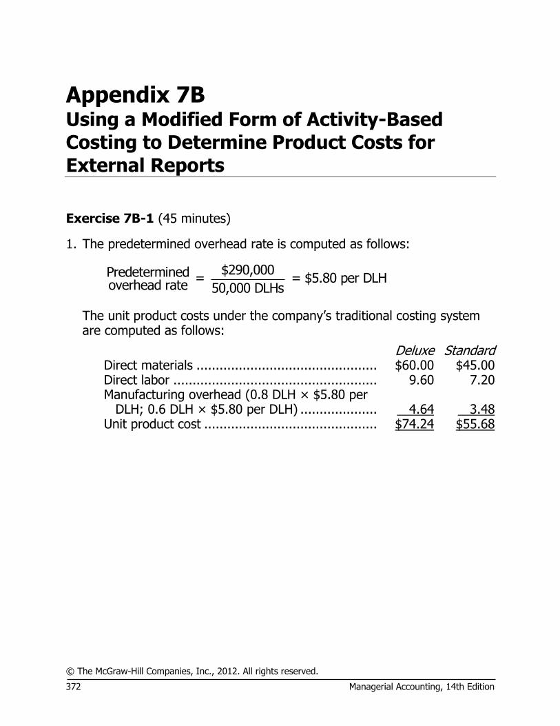
© The McGraw-Hill Companies, Inc., 2012. All rights reserved. 372 Managerial Accounting, 14th Edition
Appendix 7B Using a Modified Form of Activity-Based Costing to Determine Product Costs for External Reports
Exercise 7B-1 (45 minutes)
1. The predetermined overhead rate is computed as follows:
$290,000Predetermined = = $5.80 per DLHoverhead rate 50,000 DLHs
The unit product costs under the company’s traditional costing system are computed as follows:
Deluxe Standard Direct materials ............................................... $60.00 $45.00 Direct labor ..................................................... 9.60 7.20 Manufacturing overhead (0.8 DLH × $5.80 per
DLH; 0.6 DLH × $5.80 per DLH) .................... 4.64 3.48 Unit product cost ............................................. $74.24 $55.68
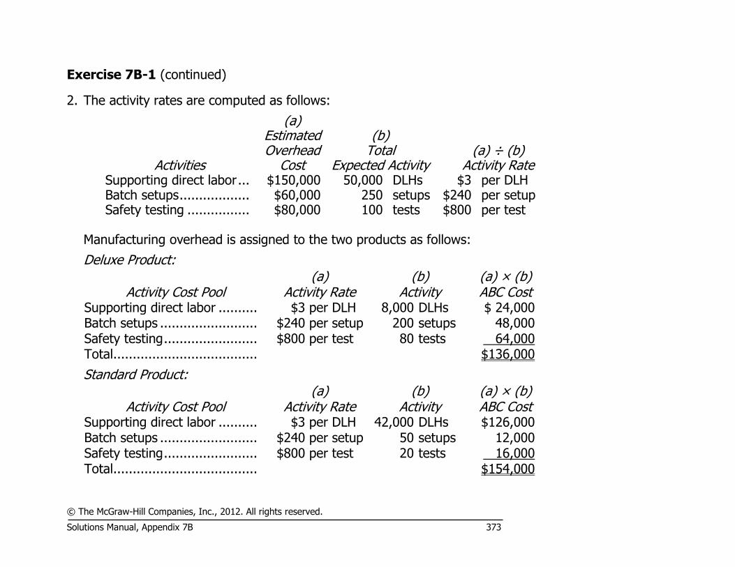
© The McGraw-Hill Companies, Inc., 2012. All rights reserved. Solutions Manual, Appendix 7B 373
Exercise 7B-1 (continued)
2. The activity rates are computed as follows:
(a) Estimated (b) Overhead Total (a) ÷ (b)
Activities Cost Expected Activity Activity Rate Supporting direct labor ... $150,000 50,000 DLHs $3 per DLH Batch setups .................. $60,000 250 setups $240 per setup Safety testing ................ $80,000 100 tests $800 per test
Manufacturing overhead is assigned to the two products as follows:
Deluxe Product:
Activity Cost Pool (a)
Activity Rate (b)
Activity (a) × (b) ABC Cost
Supporting direct labor .......... $3 per DLH 8,000 DLHs $ 24,000 Batch setups ......................... $240 per setup 200 setups 48,000 Safety testing ........................ $800 per test 80 tests 64,000 Total ..................................... $136,000
Standard Product:
Activity Cost Pool (a)
Activity Rate (b)
Activity (a) × (b) ABC Cost
Supporting direct labor .......... $3 per DLH 42,000 DLHs $126,000 Batch setups ......................... $240 per setup 50 setups 12,000 Safety testing ........................ $800 per test 20 tests 16,000 Total ..................................... $154,000

© The McGraw-Hill Companies, Inc., 2012. All rights reserved. 374 Managerial Accounting, 14th Edition
Exercise 7B-1 (continued)
Activity-based costing unit product costs are computed as follows:
Deluxe Standard Direct materials ................................................... $60.00 $45.00 Direct labor ......................................................... 9.60 7.20 Manufacturing overhead ($136,000 ÷ 10,000
units; $154,000 ÷ 70,000 units) ........................ 13.60 2.20 Unit product cost ................................................. $83.20 $54.40

© The McGraw-Hill Companies, Inc., 2012. All rights reserved. Solutions Manual, Appendix 7B 375
Exercise 7-B2 (45 minutes)
1. The unit product costs under the company's conventional costing system would be computed as follows:
Mercon Wurcon Total
Number of units produced (a) ................... 10,000 40,000 Direct labor-hours per unit (b) ................... 0.20 0.25 Total direct labor-hours (a) × (b) .............. 2,000 10,000 12,000
Total manufacturing overhead (a) ............. $336,000 Total direct labor-hours (b) ....................... 12,000 DLHs Predetermined overhead rate (a) ÷ (b) ...... $28.00 per DLH
Mercon Wurcon Direct materials ........................................ $10.00 $ 8.00 Direct labor .............................................. 3.00 3.75 Manufacturing overhead applied:
0.20 DLH per unit × $28.00 per DLH ....... 5.60 0.25 DLH per unit × $28.00 per DLH ....... 7.00
Unit product cost ...................................... $18.60 $18.75
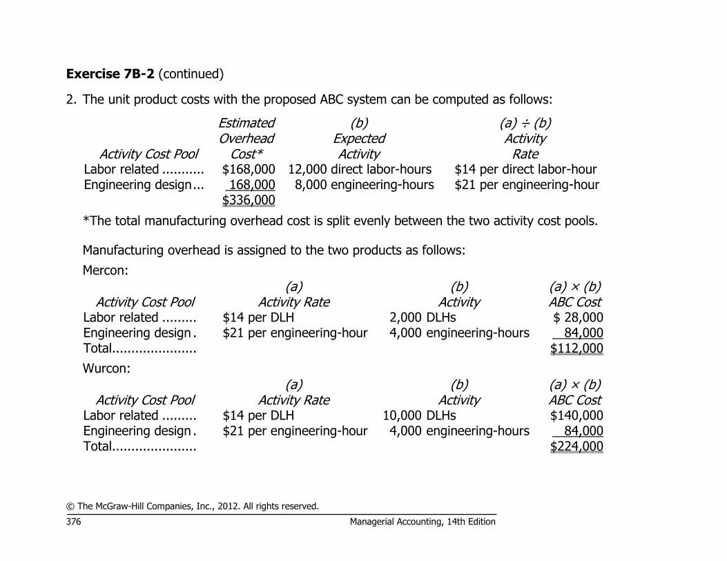
© The McGraw-Hill Companies, Inc., 2012. All rights reserved. 376 Managerial Accounting, 14th Edition
Exercise 7B-2 (continued)
2. The unit product costs with the proposed ABC system can be computed as follows:
Activity Cost Pool
Estimated Overhead
Cost*
(b) Expected Activity
(a) ÷ (b) Activity Rate
Labor related ........... $168,000 12,000 direct labor-hours $14 per direct labor-hour Engineering design ... 168,000 8,000 engineering-hours $21 per engineering-hour $336,000
*The total manufacturing overhead cost is split evenly between the two activity cost pools. Manufacturing overhead is assigned to the two products as follows:
Mercon:
Activity Cost Pool (a)
Activity Rate (b)
Activity (a) × (b) ABC Cost
Labor related ......... $14 per DLH 2,000 DLHs $ 28,000 Engineering design . $21 per engineering-hour 4,000 engineering-hours 84,000 Total ...................... $112,000
Wurcon:
Activity Cost Pool (a)
Activity Rate (b)
Activity (a) × (b) ABC Cost
Labor related ......... $14 per DLH 10,000 DLHs $140,000 Engineering design . $21 per engineering-hour 4,000 engineering-hours 84,000 Total ...................... $224,000

© The McGraw-Hill Companies, Inc., 2012. All rights reserved. Solutions Manual, Appendix 7B 377
Exercise 7B-2 (continued)
The unit product costs combine direct materials, direct labor, and manufacturing overhead costs:
Mercon Wurcon Direct materials ............................................. $10.00 $ 8.00 Direct labor ................................................... 3.00 3.75 Manufacturing overhead ($112,000 ÷ 10,000
units; $224,000 ÷ 40,000 units) .................. 11.20 5.60 Unit product cost ........................................... $24.20 $17.35
3. The unit product cost of the high-volume product, Wurcon, declines
under the activity-based costing system, whereas the unit product cost of the low-volume product, Mercon, increases. This occurs because half of the overhead is applied on the basis of engineering design hours instead of direct labor-hours. When the overhead was applied on the basis of direct labor-hours, most of the overhead was applied to the high-volume product. However, when the overhead is applied on the basis of engineering-hours, more of the overhead cost is shifted over to the low-volume product. Engineering design is a product-level activity, so the higher the volume, the lower the unit cost and the lower the volume, the higher the unit cost.

© The McGraw-Hill Companies, Inc., 2012. All rights reserved. 378 Managerial Accounting, 14th Edition
Problem 7B-3 (60 minutes)
1. The company’s estimated direct labor-hours (DLHs) can be computed as follows:
Deluxe model: 15,000 units × 1.6 DLH per unit .... 24,000 Regular model: 120,000 units × 0.8 DLH per unit . 96,000 Total direct labor-hours ....................................... 120,000
Using direct labor-hours as the base, the predetermined overhead rate would be:
Estimated overhead cost $6,000,000= =$50 per DLHEstimated direct labor-hours 120,000 DLHs
The unit product cost of each model using the company’s traditional costing system would be:
Deluxe Regular Direct materials ................. $154 $112 Direct labor ....................... 16 8 Manufacturing overhead:
$50 per DLH × 1.6 DLHs . 80 $50 per DLH × 0.8 DLHs . 40
Total unit product cost ....... $250 $160
2. Predetermined overhead rates are computed below:
Activity Cost Pool
(a) Estimated Overhead
Cost
(b) Expected Activity
(a) ÷ (b) Predetermined Overhead Rate
Purchase orders ........ $252,000 1,200 purchase orders
$210 per purchase order
Scrap/rework orders .. $648,000 900 scrap/rework
orders
$720 per scrap/ rework order
Product testing .......... $1,350,000 15,000 tests $90 per test Machine related ........ $3,750,000 50,000 MHs $75 per MH
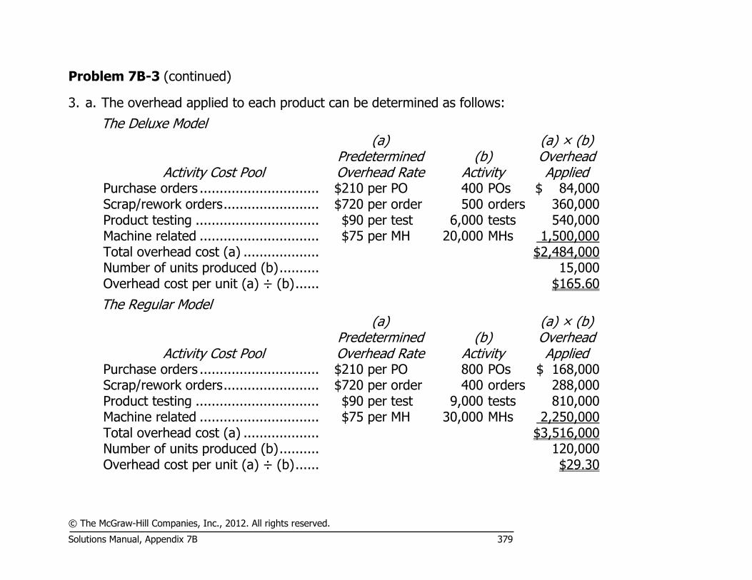
© The McGraw-Hill Companies, Inc., 2012. All rights reserved. Solutions Manual, Appendix 7B 379
Problem 7B-3 (continued)
3. a. The overhead applied to each product can be determined as follows:
The Deluxe Model
Activity Cost Pool
(a) Predetermined Overhead Rate
(b) Activity
(a) × (b) Overhead Applied
Purchase orders .............................. $210 per PO 400 POs $ 84,000 Scrap/rework orders ........................ $720 per order 500 orders 360,000 Product testing ............................... $90 per test 6,000 tests 540,000 Machine related .............................. $75 per MH 20,000 MHs 1,500,000 Total overhead cost (a) ................... $2,484,000 Number of units produced (b) .......... 15,000 Overhead cost per unit (a) ÷ (b) ...... $165.60
The Regular Model
Activity Cost Pool
(a) Predetermined Overhead Rate
(b) Activity
(a) × (b) Overhead Applied
Purchase orders .............................. $210 per PO 800 POs $ 168,000 Scrap/rework orders ........................ $720 per order 400 orders 288,000 Product testing ............................... $90 per test 9,000 tests 810,000 Machine related .............................. $75 per MH 30,000 MHs 2,250,000 Total overhead cost (a) ................... $3,516,000 Number of units produced (b) .......... 120,000 Overhead cost per unit (a) ÷ (b) ...... $29.30

© The McGraw-Hill Companies, Inc., 2012. All rights reserved. 380 Managerial Accounting, 14th Edition
Problem 7B-3 (continued)
b. Using activity-based costing, the unit product cost of each model would be:
Deluxe Regular Direct materials ............................ $154.00 $112.00 Direct labor .................................. 16.00 8.00 Manufacturing overhead (above) ... 165.60 29.30 Total unit product cost .................. $335.60 $149.30
4. It is risky to draw any definite conclusions based on the above analysis.
The activity-based costing system used in this company is not completely suitable for making decisions. Product costs probably include the costs of idle capacity and organization-sustaining costs. They also exclude nonmanufacturing costs that may be caused by the products. Nevertheless, the above analysis is suggestive. Unit costs appear to be distorted as a result of using direct labor-hours as the base for assigning overhead cost to products. Although the deluxe model requires twice as much labor time as the regular model, it still is not being assigned enough overhead cost, as shown in the analysis in part 3(a).
When the company’s overhead costs are analyzed on an activities basis, it appears that the deluxe model is more expensive to manufacture than the company realizes. Note that the deluxe model accounts for 40% of the machine-hours, although it represents a small part of the company’s total production. Also, it consumes a disproportionately large amount of the activities.
When activity-based costing is used in place of direct labor as the basis for assigning overhead cost to products, the unit product cost of the deluxe model jumps from $250 to $335.60. If the $250 cost figure is being used as the basis for pricing, then the selling price for the deluxe model may be too low. This may be one reason why profits have been declining over the last several years. It may also be the reason why sales of the deluxe model have been increasing rapidly.
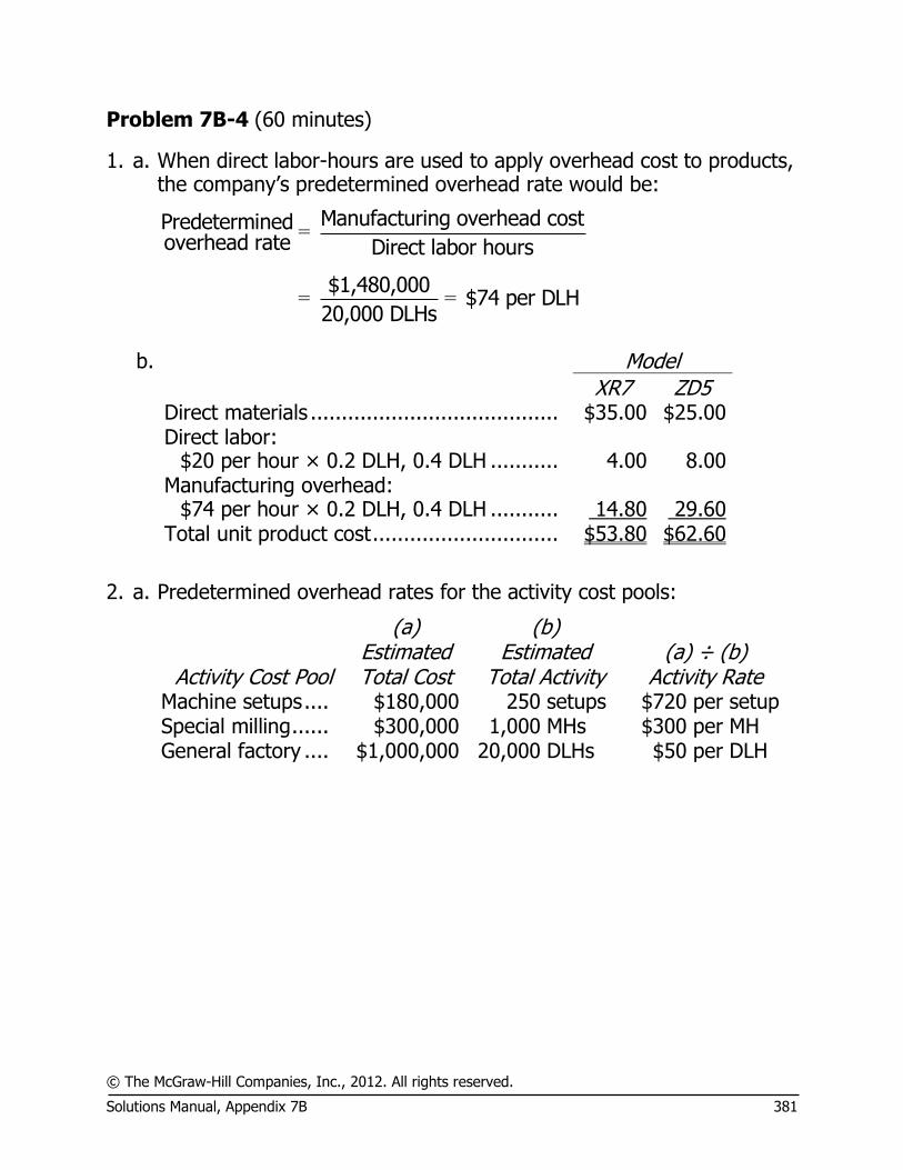
© The McGraw-Hill Companies, Inc., 2012. All rights reserved. Solutions Manual, Appendix 7B 381
Problem 7B-4 (60 minutes)
1. a. When direct labor-hours are used to apply overhead cost to products, the company’s predetermined overhead rate would be:
Manufacturing overhead costPredeterminedoverhead rate Direct labor hours
$1,480,000 $74 per DLH20,000 DLHs
=
= =
b. Model XR7 ZD5 Direct materials ........................................ $35.00 $25.00
Direct labor:
$20 per hour × 0.2 DLH, 0.4 DLH ........... 4.00 8.00
Manufacturing overhead:
$74 per hour × 0.2 DLH, 0.4 DLH ........... 14.80 29.60 Total unit product cost .............................. $53.80 $62.60
2. a. Predetermined overhead rates for the activity cost pools:
Activity Cost Pool
(a) Estimated Total Cost
(b) Estimated
Total Activity (a) ÷ (b)
Activity Rate Machine setups .... $180,000 250 setups $720 per setup Special milling ...... $300,000 1,000 MHs $300 per MH General factory .... $1,000,000 20,000 DLHs $50 per DLH
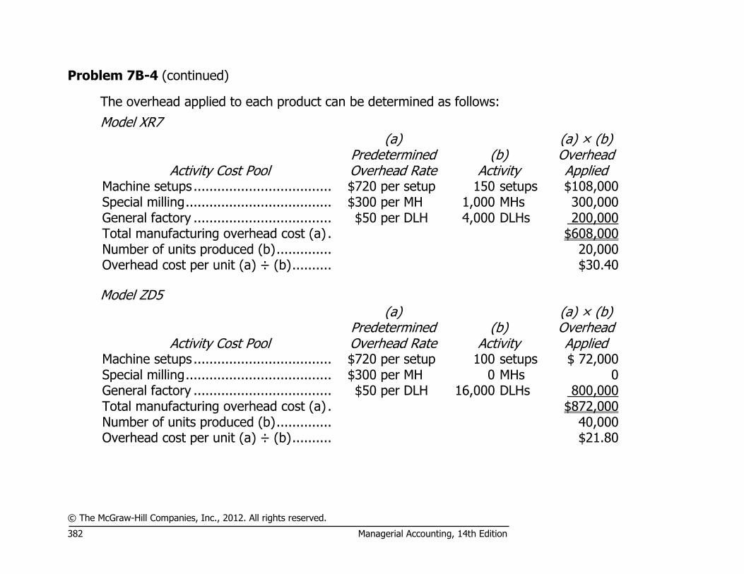
© The McGraw-Hill Companies, Inc., 2012. All rights reserved. 382 Managerial Accounting, 14th Edition
Problem 7B-4 (continued)
The overhead applied to each product can be determined as follows:
Model XR7
Activity Cost Pool
(a) Predetermined Overhead Rate
(b) Activity
(a) × (b) Overhead Applied
Machine setups ................................... $720 per setup 150 setups $108,000 Special milling ..................................... $300 per MH 1,000 MHs 300,000 General factory ................................... $50 per DLH 4,000 DLHs 200,000 Total manufacturing overhead cost (a) . $608,000 Number of units produced (b) .............. 20,000 Overhead cost per unit (a) ÷ (b) .......... $30.40 Model ZD5
Activity Cost Pool
(a) Predetermined Overhead Rate
(b) Activity
(a) × (b) Overhead Applied
Machine setups ................................... $720 per setup 100 setups $ 72,000 Special milling ..................................... $300 per MH 0 MHs 0 General factory ................................... $50 per DLH 16,000 DLHs 800,000 Total manufacturing overhead cost (a) . $872,000 Number of units produced (b) .............. 40,000 Overhead cost per unit (a) ÷ (b) .......... $21.80

© The McGraw-Hill Companies, Inc., 2012. All rights reserved. Solutions Manual, Appendix 7B 383
Problem 7B-4 (continued)
b. The unit product cost of each model under activity-based costing would be computed as follows:
Model XR7 ZD5 Direct materials .............................................. $35.00 $25.00 Direct labor ($20 per DLH × 0.2 DLH; $20 per
DLH × 04.DLH) ............................................ 4.00 8.00 Manufacturing overhead (above) ..................... 30.40 21.80 Total unit product cost .................................... $69.40 $54.80
Comparing these unit cost figures with the unit costs in Part 1(b), we find that the unit product cost for Model XR7 has increased from $53.80 to $69.40, and the unit product cost for Model ZD5 has decreased from $62.60 to $54.80.
3. It is especially important to note that, even under activity-based costing,
68% of the company’s overhead costs continue to be applied to products on the basis of direct labor-hours:
Machine setups (number of setups) ... $ 180,000 12 % Special milling (machine-hours) ......... 300,000 20 General factory (direct labor-hours) ... 1,000,000 68 Total overhead cost .......................... $1,480,000 100 %
Thus, the shift in overhead cost from the high-volume product (Model ZD5) to the low-volume product (Model XR7) occurred as a result of reassigning only 32% of the company’s overhead costs.
The increase in unit product cost for Model XR7 can be explained as follows: First, where possible, overhead costs have been traced to the products rather than being lumped together and spread uniformly over production. Therefore, the special milling costs, which are traceable to Model XR7, have all been assigned to Model XR7 and none assigned to Model ZD5 under the activity-based costing approach. It is common in industry to have some products that require special handling or special milling of some type. This is especially true in modern factories that produce a variety of products. Activity-based costing provides a vehicle for assigning these costs to the appropriate products.

© The McGraw-Hill Companies, Inc., 2012. All rights reserved. 384 Managerial Accounting, 14th Edition
Problem 7B-4 (continued)
Second, the costs associated with the batch-level activity (machine setups) have also been assigned to the specific products to which they relate. These costs have been assigned according to the number of setups completed for each product. However, because a batch-level activity is involved, another factor affecting unit costs comes into play. That factor is batch size. Some products are produced in large batches and some are produced in small batches. The smaller the batch, the higher the cost per unit of the batch activity. In the case at hand, the data can be analyzed as shown below.
Model XR7: Cost to complete one setup [see 2(a)] ......... $720 (a) Number of units processed per setup
(20,000 units ÷ 150 setups) ..................... 133.33 (b) Setup cost per unit (a) ÷ (b) ....................... $5.40
Model ZD5:
Cost to complete one setup (above) ............ $720 (a) Number of units processed per setup
(40,000 units ÷ 100 setups) ..................... 400 (b) Setup cost per unit (a) ÷ (b) ....................... $1.80
Thus, the cost per unit for setups is three times as great for Model XR7, the low-volume product, as it is for Model ZD5, the high-volume product. Such differences in cost are obscured when direct labor-hours (or any other volume measure) is used as the basis for applying overhead cost to products.
In sum, overhead cost has shifted from the high-volume product to the low-volume product as a result of more appropriately assigning some costs to the products on the basis of the activities involved, rather than on the basis of direct labor-hours.

© The McGraw-Hill Companies, Inc., 2012. All rights reserved. Solutions Manual, Appendix 7B 385
Case 7B-5 (90 minutes)
1. a. The predetermined overhead rate would be computed as follows: Expected manufacturing overhead cost $3,000,000=
Estimated direct labor-hours 50,000 DLHs
=$60 per DLH
b. The unit product cost per pound, using the company’s present costing system, would be:
Mona Loa Malaysian Direct materials (given) ........... $4.20 $3.20 Direct labor (given) ................. 0.30 0.30 Manufacturing overhead:
0.025 DLH × $60 per DLH ..... 1.50 1.50 Total unit product cost ............. $6.00 $5.00
2. a. Overhead rates by activity center:
Activity Center
(a) Estimated Overhead
Costs
(b) Expected Activity
(a) ÷ (b) Predetermined Overhead Rate
Purchasing ........... $513,000 1,710 orders $300 per order Material handling .. $720,000 1,800 setups $400 per setup Quality control ...... $144,000 600 batches $240 per batch Roasting ............... $961,000 96,100 hours $10 per hour Blending ............... $402,000 33,500 hours $12 per hour Packaging ............. $260,000 26,000 hours $10 per hour

© The McGraw-Hill Companies, Inc., 2012. All rights reserved. 386 Managerial Accounting, 14th Edition
Case 7B-5 (continued)
Before we can determine the amount of overhead cost to assign to the products we must first determine the activity for each of the products in the six activity centers. The necessary computations follow:
Number of purchase orders: Mona Loa: 100,000 pounds ÷ 20,000 pounds per order = 5 orders Malaysian: 2,000 pounds ÷ 500 pounds per order = 4 orders
Number of batches: Mona Loa: 100,000 pounds ÷ 10,000 pounds per batch = 10 batches Malaysian: 2,000 pounds ÷ 500 pounds per batch = 4 batches
Number of setups: Mona Loa: 10 batches × 3 setups per batch = 30 setups Malaysian: 4 batches × 3 setups per batch = 12 setups
Roasting hours: Mona Loa: 1 hour × (100,000 pounds ÷ 100 pounds) = 1,000 hours Malaysian: 1 hour × (2,000 pounds ÷ 100 pounds) = 20 hours
Blending hours: Mona Loa: 0.5 hour × (100,000 pounds ÷ 100 pounds) = 500 hours Malaysian: 0.5 hour × (2,000 pounds ÷ 100 pounds) = 10 hours
Packaging hours: Mona Loa: 0.1 hour × (100,000 pounds ÷ 100 pounds) = 100 hours Malaysian: 0.1 hour × (2,000 pounds ÷ 100 pounds) = 2 hours

© The McGraw-Hill Companies, Inc., 2012. All rights reserved. Solutions Manual, Appendix 7B 387
Case 7B-5 (continued)
The overhead applied to each product can be determined as follows:
Mona Loa
Activity Cost Pool
(a) Predetermined Overhead Rate
(b) Activity
(a) × (b) Overhead Applied
Purchasing ............. $300 per order 5 orders $ 1,500 Material handling ... $400 per setup 30 setups 12,000 Quality control ....... $240 per batch 10 batches 2,400 Roasting ................ $10 per roasting hour 1,000 roasting hours 10,000 Blending ................ $12 per blending hour 500 blending hours 6,000 Packaging .............. $10 per packaging hour 100 packaging hours 1,000 Total ..................... $32,900 Malaysian
Activity Cost Pool
(a) Predetermined Overhead Rate
(b) Activity
(a) × (b) Overhead Applied
Purchasing ............. $300 per order 4 orders $1,200 Material handling ... $400 per setup 12 setups 4,800 Quality control ....... $240 per batch 4 batches 960 Roasting ................ $10 per roasting hour 20 roasting hours 200 Blending ................ $12 per blending hour 10 blending hours 120 Packaging .............. $10 per packaging hour 2 packaging hours 20 Total ..................... $7,300

© The McGraw-Hill Companies, Inc., 2012. All rights reserved. 388 Managerial Accounting, 14th Edition
Case 7B-5 (continued)
b. According to the activity-based costing system, the manufacturing overhead cost per pound is:
Mona Loa Malaysian Total overhead cost assigned (above) (a) ... $32,900 $7,300 Number of pounds manufactured (b) .......... 100,000 2,000 Cost per pound (a) ÷ (b) ........................... $0.33 $3.65
c. The unit product costs according to the activity-based costing system
are: Mona Loa Malaysian Direct materials (given) ......... $4.20 $3.20 Direct labor (given) ............... 0.30 0.30 Manufacturing overhead ........ 0.33 3.65 Total unit product cost ........... $4.83 $7.15
3. MEMO TO THE PRESIDENT: Analysis of CBI’s data shows that several
activities other than direct labor drive the company’s manufacturing overhead costs. These activities include purchase orders issued, number of setups for material processing, and number of batches processed. The company’s present costing system, which relies on direct labor time as the sole basis for assigning overhead cost to products, significantly undercosts low-volume products, such as the Malaysian coffee, and significantly overcosts high-volume products, such as our Mona Loa coffee.
An implication of the activity-based costing analysis is that our low-volume products may not be covering the costs of the manufacturing resources they use. For example, Malaysian coffee is currently priced at $6.50 per pound, but this price is significantly below its activity-based cost of $7.15 per pound. Under our present costing and pricing system, our high-volume products, such as our Mona Loa coffee, may be subsidizing our low-volume products. Some adjustments in prices may be required. However, before taking such an action, an action analysis report (discussed in Appendix 7A) should be prepared.

© The McGraw-Hill Companies, Inc., 2012. All rights reserved. Solutions Manual, Appendix 7B 389
Case 7B-5 (continued)
ALTERNATIVE SOLUTION:
Many students will compute the manufacturing overhead cost per pound of the two coffees as shown above. However, the cost per pound can also be computed as shown below. This alternative approach provides additional insight into the data and facilitates emphasis of some points made in the chapter.
Mona Loa Malaysian
Total Per Pound
(÷ 100,000) Total Per Pound (÷ 2,000)
Purchasing ........... $ 1,500 $0.015 $1,200 $0.600 Material handling .. 12,000 0.120 4,800 2.400 Quality control ...... 2,400 0.024 960 0.480 Roasting .............. 10,000 0.100 200 0.100 Blending .............. 6,000 0.060 120 0.060 Packaging ............ 1,000 0.010 20 0.010 Total .................... $32,900 $0.329 $7,300 $3.650
Note particularly how batch size impacts unit cost data. For example, the cost to the company to process a purchase order is $300, regardless of how many pounds of coffee are contained in the order. Twenty thousand pounds of the Mona Loa coffee are purchased per order (with five orders per year), and just 500 pounds of the Malaysian coffee are purchased per order (with four orders per year). Thus, the purchase order cost per pound for the Mona Loa coffee is just 1.5 cents, whereas the purchase order cost per pound for the Malaysian coffee is 40 times as much, or 60 cents. As stated in the text, this is one reason why unit costs of low-volume products, such as the Malaysian coffee, increase so dramatically when activity-based costing is used.
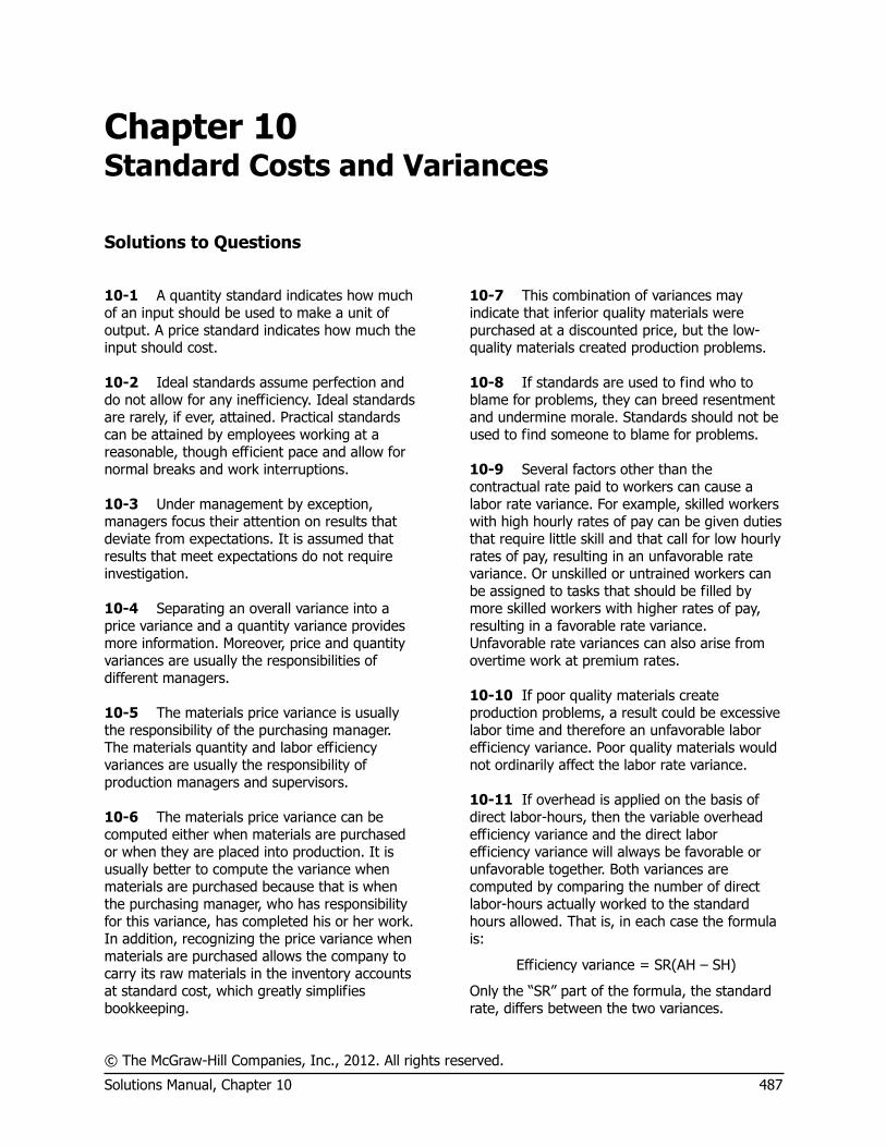
© The McGraw-Hill Companies, Inc., 2012. All rights reserved.
Solutions Manual, Chapter 10 487
Chapter 10 Standard Costs and Variances
Solutions to Questions
10-1 A quantity standard indicates how much of an input should be used to make a unit of output. A price standard indicates how much the input should cost.
10-2 Ideal standards assume perfection and do not allow for any inefficiency. Ideal standards are rarely, if ever, attained. Practical standards can be attained by employees working at a reasonable, though efficient pace and allow for normal breaks and work interruptions.
10-3 Under management by exception, managers focus their attention on results that deviate from expectations. It is assumed that results that meet expectations do not require investigation.
10-4 Separating an overall variance into a price variance and a quantity variance provides more information. Moreover, price and quantity variances are usually the responsibilities of different managers.
10-5 The materials price variance is usually the responsibility of the purchasing manager. The materials quantity and labor efficiency variances are usually the responsibility of production managers and supervisors.
10-6 The materials price variance can be computed either when materials are purchased or when they are placed into production. It is usually better to compute the variance when materials are purchased because that is when the purchasing manager, who has responsibility for this variance, has completed his or her work. In addition, recognizing the price variance when materials are purchased allows the company to carry its raw materials in the inventory accounts at standard cost, which greatly simplifies bookkeeping.
10-7 This combination of variances may indicate that inferior quality materials were purchased at a discounted price, but the low-quality materials created production problems.
10-8 If standards are used to find who to blame for problems, they can breed resentment and undermine morale. Standards should not be used to find someone to blame for problems.
10-9 Several factors other than the contractual rate paid to workers can cause a labor rate variance. For example, skilled workers with high hourly rates of pay can be given duties that require little skill and that call for low hourly rates of pay, resulting in an unfavorable rate variance. Or unskilled or untrained workers can be assigned to tasks that should be filled by more skilled workers with higher rates of pay, resulting in a favorable rate variance. Unfavorable rate variances can also arise from overtime work at premium rates.
10-10 If poor quality materials create production problems, a result could be excessive labor time and therefore an unfavorable labor efficiency variance. Poor quality materials would not ordinarily affect the labor rate variance.
10-11 If overhead is applied on the basis of direct labor-hours, then the variable overhead efficiency variance and the direct labor efficiency variance will always be favorable or unfavorable together. Both variances are computed by comparing the number of direct labor-hours actually worked to the standard hours allowed. That is, in each case the formula is:
Efficiency variance = SR(AH – SH)
Only the “SR” part of the formula, the standard rate, differs between the two variances.
© The McGraw-Hill Companies, Inc., 2012
488 Managerial Accounting, 14th Edition
10-12 A statistical control chart is a graphical aid that helps identify variances that should be investigated. Upper and lower limits are set on the control chart. Any variances falling between those limits are considered to be normal. Any variances falling outside of those limits are considered abnormal and are investigated.
10-13 If labor is a fixed cost and standards are tight, then the only way to generate favorable labor efficiency variances is for every workstation to produce at capacity. However, the
output of the entire system is limited by the capacity of the bottleneck. If workstations before the bottleneck in the production process produce at capacity, the bottleneck will be unable to process all of the work in process. In general, if every workstation is attempting to produce at capacity, then work in process inventory will build up in front of the workstations with the least capacity.

© The McGraw-Hill Companies, Inc., 2012. All rights reserved.
Solutions Manual, Chapter 10 489
Exercise 10-1 (20 minutes)
1. Number of chopping blocks .................................. 4,000 Number of board feet per chopping block ............. × 2.5 Standard board feet allowed ................................ 10,000 Standard cost per board foot................................ × $1.80 Total standard cost .............................................. $18,000
Actual cost incurred ............................................. $18,700 Standard cost above ............................................ 18,000 Spending variance—unfavorable ........................... $ 700
2. Standard Quantity Allowed
for Actual Output, at Standard Price
(SQ × SP)
Actual Quantity of Input,
at Standard Price (AQ × SP)
Actual Quantity of Input,
at Actual Price (AQ × AP)
10,000 board feet × $1.80 per board foot
= $18,000
11,000 board feet × $1.80 per board foot
= $19,800 $18,700
Materials quantity variance = $1,800 U
Materials price variance = $1,100 F
Spending variance = $700 U Alternatively, the variances can be computed using the formulas:
Materials quantity variance = SP (AQ – SQ) = $1.80 per board foot (11,000 board feet – 10,000 board feet) = $1,800 U
Materials price variance = AQ (AP – SP) = 11,000 board feet ($1.70 per board foot* – $1.80 per board foot) = $1,100 F *$18,700 ÷ 11,000 board feet = $1.70 per board foot.
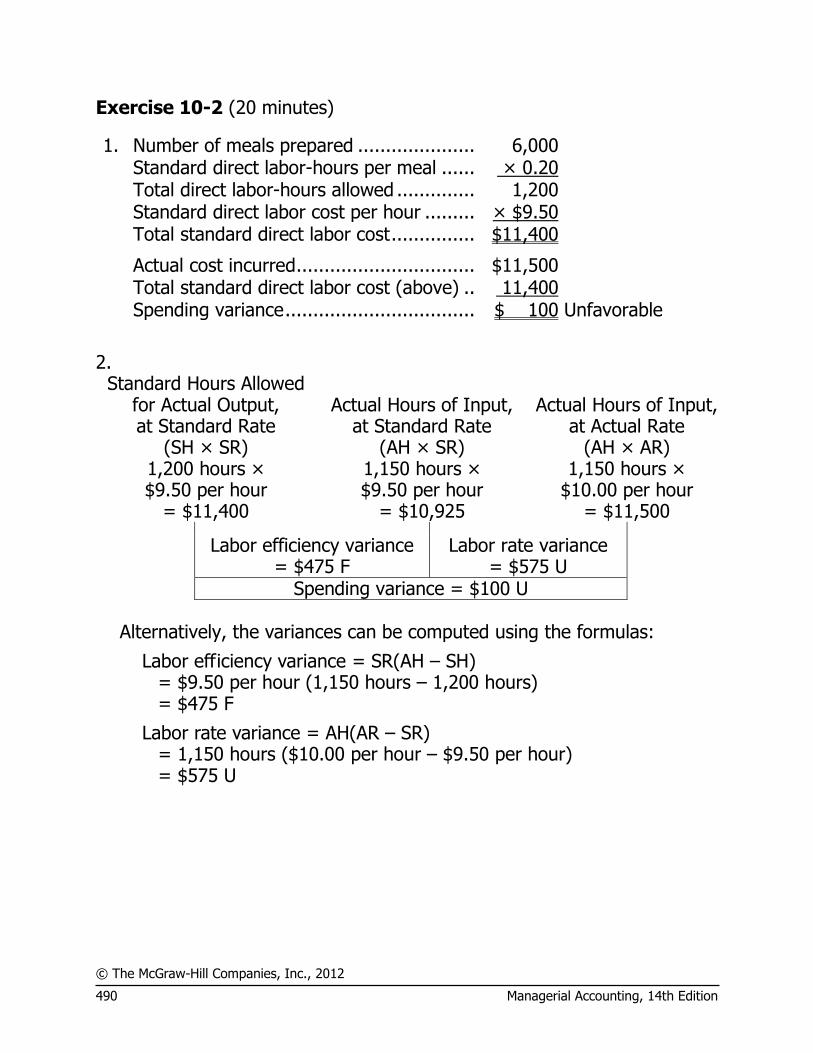
© The McGraw-Hill Companies, Inc., 2012
490 Managerial Accounting, 14th Edition
Exercise 10-2 (20 minutes)
1. Number of meals prepared ..................... 6,000 Standard direct labor-hours per meal ...... × 0.20 Total direct labor-hours allowed .............. 1,200 Standard direct labor cost per hour ......... × $9.50 Total standard direct labor cost ............... $11,400
Actual cost incurred ................................ $11,500 Total standard direct labor cost (above) .. 11,400 Spending variance .................................. $ 100 Unfavorable
2. Standard Hours Allowed
for Actual Output, at Standard Rate
(SH × SR)
Actual Hours of Input, at Standard Rate
(AH × SR)
Actual Hours of Input, at Actual Rate
(AH × AR) 1,200 hours × $9.50 per hour
= $11,400
1,150 hours × $9.50 per hour
= $10,925
1,150 hours × $10.00 per hour
= $11,500
Labor efficiency variance = $475 F
Labor rate variance = $575 U
Spending variance = $100 U Alternatively, the variances can be computed using the formulas:
Labor efficiency variance = SR(AH – SH) = $9.50 per hour (1,150 hours – 1,200 hours) = $475 F
Labor rate variance = AH(AR – SR) = 1,150 hours ($10.00 per hour – $9.50 per hour) = $575 U

© The McGraw-Hill Companies, Inc., 2012. All rights reserved.
Solutions Manual, Chapter 10 491
Exercise 10-3 (20 minutes)
1. Number of items shipped ................................. 140,000 Standard direct labor-hours per item ................ × 0.04 Total direct labor-hours allowed ....................... 5,600 Standard variable overhead cost per hour ......... × $2.80 Total standard variable overhead cost .............. $15,680
Actual variable overhead cost incurred ............. $15,950 Total standard variable overhead cost (above) .. 15,680 Spending variance ........................................... $ 270 Unfavorable
2. Standard Hours Allowed
for Actual Output, at Standard Rate
(SH × SR)
Actual Hours of Input, at Standard Rate
(AH × SR)
Actual Hours of Input, at Actual Rate
(AH × AR) 5,600 hours × $2.80 per hour
= $15,680
5,800 hours × $2.80 per hour
= $16,240
5,800 hours × $2.75 per hour*
= $15,950
Variable overhead efficiency variance
= $560 U
Variable overhead rate variance
= $290 F
Spending variance = $270 U
*$15,950 ÷ 5,800 hours = $2.75 per hour Alternatively, the variances can be computed using the formulas:
Variable overhead efficiency variance = SR(AH – SH) = $2.80 per hour (5,800 hours – 5,600 hours) = $560 U
Variable overhead rate variance = AH(AR – SR) = 5,800 hours ($2.75 per hour – $2.80 per hour) = $290 F
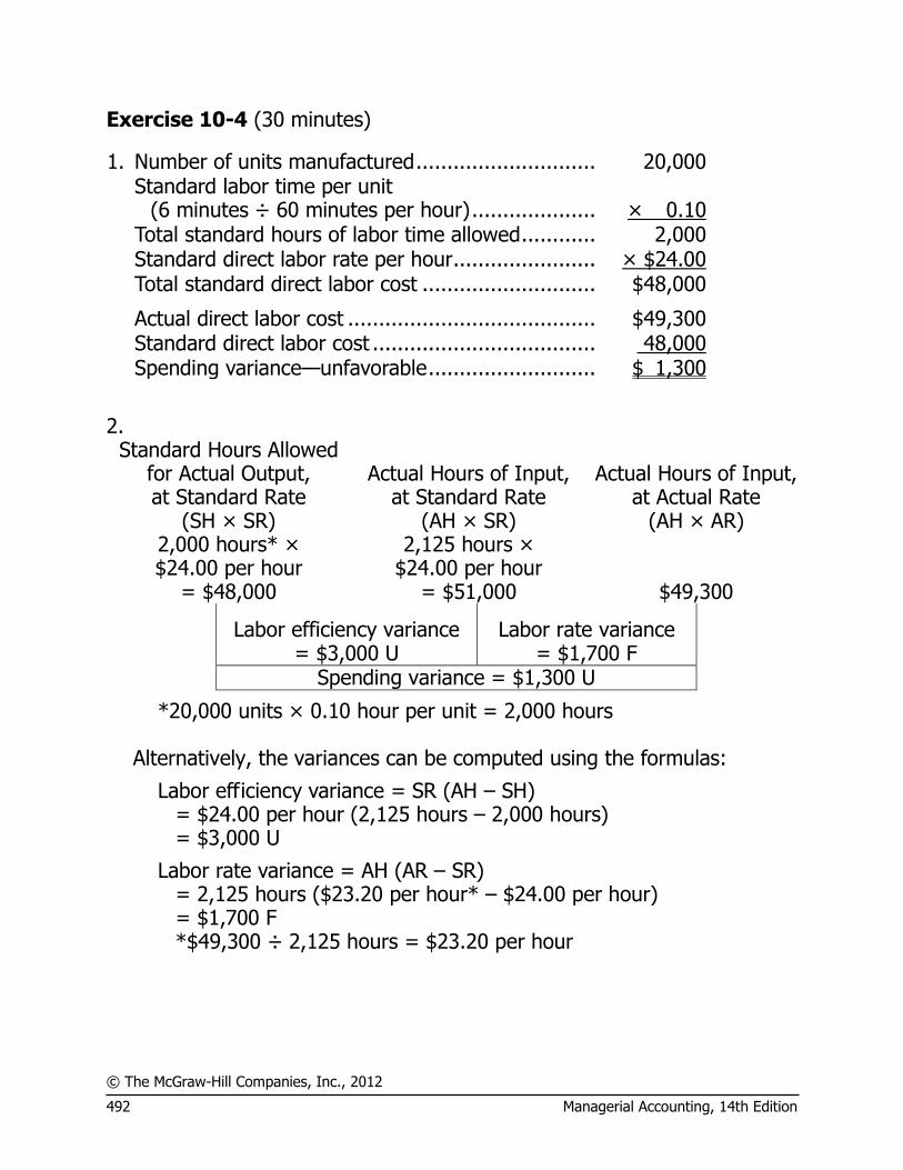
© The McGraw-Hill Companies, Inc., 2012
492 Managerial Accounting, 14th Edition
Exercise 10-4 (30 minutes)
1. Number of units manufactured ............................. 20,000
Standard labor time per unit
(6 minutes ÷ 60 minutes per hour) .................... × 0.10 Total standard hours of labor time allowed ............ 2,000 Standard direct labor rate per hour ....................... × $24.00 Total standard direct labor cost ............................ $48,000
Actual direct labor cost ........................................ $49,300 Standard direct labor cost .................................... 48,000 Spending variance—unfavorable ........................... $ 1,300
2. Standard Hours Allowed
for Actual Output, at Standard Rate
(SH × SR)
Actual Hours of Input, at Standard Rate
(AH × SR)
Actual Hours of Input, at Actual Rate
(AH × AR) 2,000 hours* × $24.00 per hour
= $48,000
2,125 hours × $24.00 per hour
= $51,000 $49,300
Labor efficiency variance = $3,000 U
Labor rate variance = $1,700 F
Spending variance = $1,300 U
*20,000 units × 0.10 hour per unit = 2,000 hours Alternatively, the variances can be computed using the formulas:
Labor efficiency variance = SR (AH – SH) = $24.00 per hour (2,125 hours – 2,000 hours) = $3,000 U
Labor rate variance = AH (AR – SR) = 2,125 hours ($23.20 per hour* – $24.00 per hour) = $1,700 F *$49,300 ÷ 2,125 hours = $23.20 per hour

© The McGraw-Hill Companies, Inc., 2012. All rights reserved.
Solutions Manual, Chapter 10 493
Exercise 10-4 (continued)
3. Standard Hours Allowed
for Actual Output, at Standard Rate
(SH × SR)
Actual Hours of Input, at Standard Rate
(AH × SR)
Actual Hours of Input, at Actual Rate
(AH × AR) 2,000 hours ×
$16.00 per hour = $32,000
2,125 hours × $16.00 per hour
= $34,000 $39,100
Variable overhead efficiency variance
= $2,000 U
Variable overhead rate variance = $5,100 U
Spending variance = $7,100 U Alternatively, the variances can be computed using the formulas:
Variable overhead efficiency variance = SR (AH – SH) =$16.00 per hour (2,125 hours – 2,000 hours) = $2,000 U
Variable overhead rate variance = AH (AR – SR) = 2,125 hours ($18.40 per hour* – $16.00 per hour) = $5,100 U *$39,100 ÷ 2,125 hours = $18.40 per hour
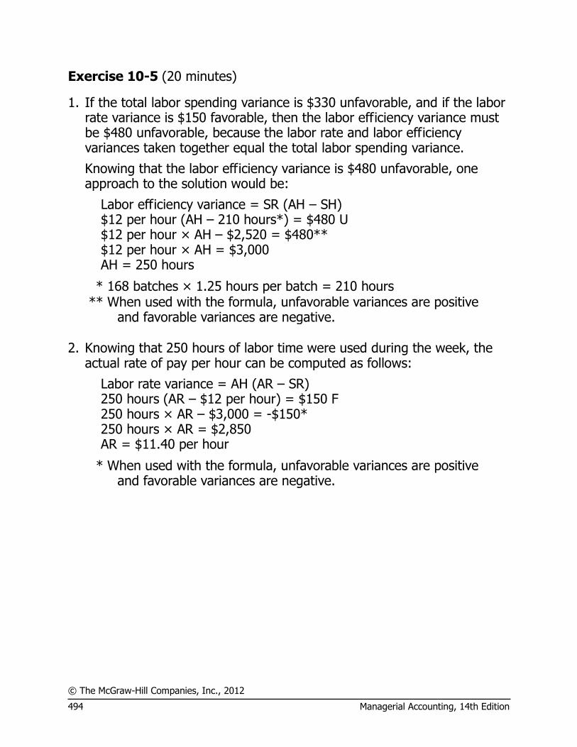
© The McGraw-Hill Companies, Inc., 2012
494 Managerial Accounting, 14th Edition
Exercise 10-5 (20 minutes)
1. If the total labor spending variance is $330 unfavorable, and if the labor rate variance is $150 favorable, then the labor efficiency variance must be $480 unfavorable, because the labor rate and labor efficiency variances taken together equal the total labor spending variance.
Knowing that the labor efficiency variance is $480 unfavorable, one approach to the solution would be:
Labor efficiency variance = SR (AH – SH) $12 per hour (AH – 210 hours*) = $480 U $12 per hour × AH – $2,520 = $480** $12 per hour × AH = $3,000 AH = 250 hours
* 168 batches × 1.25 hours per batch = 210 hours ** When used with the formula, unfavorable variances are positive
and favorable variances are negative. 2. Knowing that 250 hours of labor time were used during the week, the
actual rate of pay per hour can be computed as follows:
Labor rate variance = AH (AR – SR) 250 hours (AR – $12 per hour) = $150 F 250 hours × AR – $3,000 = -$150* 250 hours × AR = $2,850 AR = $11.40 per hour
* When used with the formula, unfavorable variances are positive and favorable variances are negative.
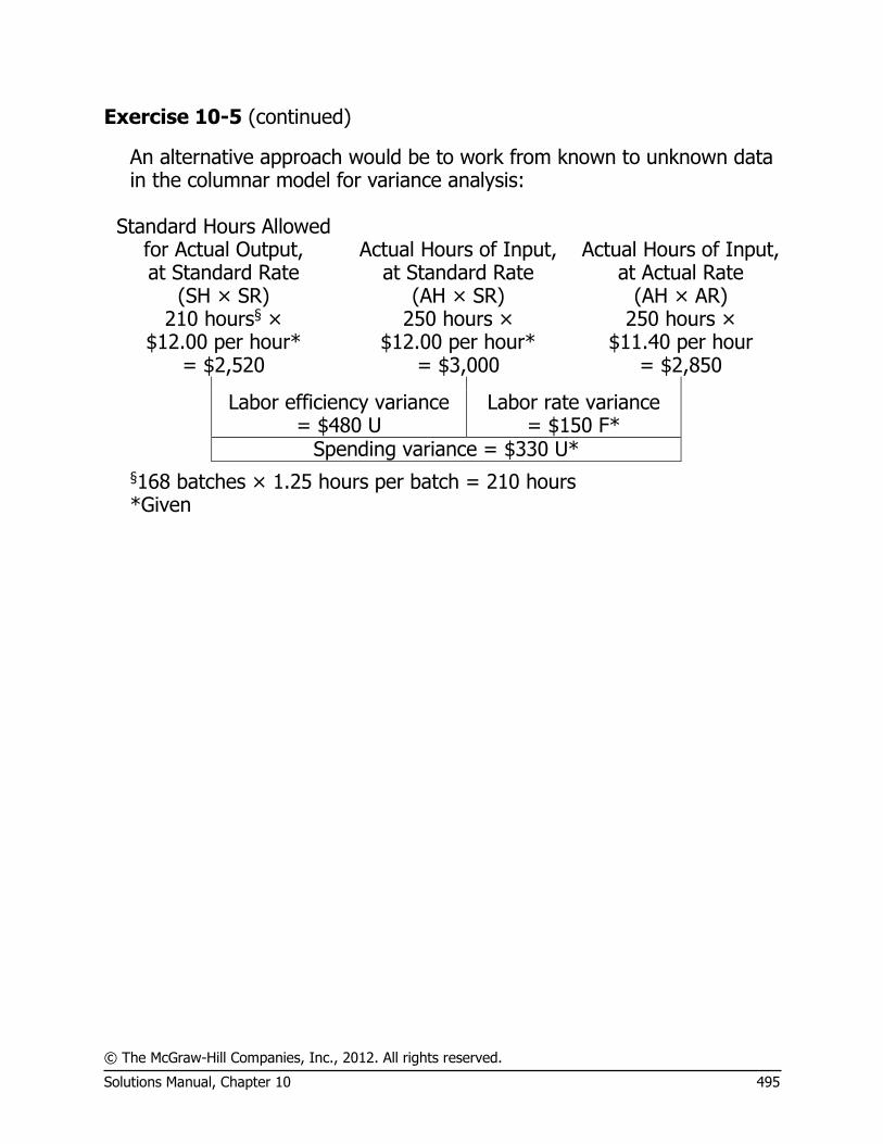
© The McGraw-Hill Companies, Inc., 2012. All rights reserved.
Solutions Manual, Chapter 10 495
Exercise 10-5 (continued)
An alternative approach would be to work from known to unknown data in the columnar model for variance analysis:
Standard Hours Allowed
for Actual Output, at Standard Rate
(SH × SR)
Actual Hours of Input, at Standard Rate
(AH × SR)
Actual Hours of Input, at Actual Rate
(AH × AR) 210 hours§ ×
$12.00 per hour* = $2,520
250 hours × $12.00 per hour*
= $3,000
250 hours × $11.40 per hour
= $2,850
Labor efficiency variance = $480 U
Labor rate variance = $150 F*
Spending variance = $330 U*
§168 batches × 1.25 hours per batch = 210 hours *Given

© The McGraw-Hill Companies, Inc., 2012
496 Managerial Accounting, 14th Edition
Exercise 10-6 (20 minutes)
1. Standard Quantity Allowed
for Actual Output, at Standard Price
(SQ × SP)
Actual Quantity of Input,
at Standard Price (AQ × SP)
Actual Quantity of Input,
at Actual Price (AQ × AP)
18,000 ounces* × $2.50 per ounce
= $45,000
20,000 ounces × $2.50 per ounce
= $50,000
20,000 ounces × $2.40 per ounce
= $48,000
Materials quantity variance = $5,000 U
Materials price variance = $2,000 F
Spending variance = $3,000 U
*2,500 units × 7.2 ounces per unit = 18,000 ounces Alternatively, the variances can be computed using the formulas:
Materials quantity variance = SP (AQ – SQ) = $2.50 per ounce (20,000 ounces – 18,000 ounces) = $5,000 U
Materials price variance = AQ (AP – SP) = 20,000 ounces ($2.40 per ounce – $2.50 per ounce) = $2,000 F
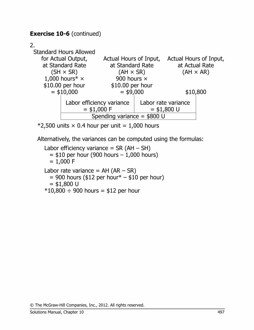
© The McGraw-Hill Companies, Inc., 2012. All rights reserved.
Solutions Manual, Chapter 10 497
Exercise 10-6 (continued)
2. Standard Hours Allowed
for Actual Output, at Standard Rate
(SH × SR)
Actual Hours of Input, at Standard Rate
(AH × SR)
Actual Hours of Input, at Actual Rate
(AH × AR) 1,000 hours* × $10.00 per hour
= $10,000
900 hours × $10.00 per hour
= $9,000 $10,800
Labor efficiency variance = $1,000 F
Labor rate variance = $1,800 U
Spending variance = $800 U
*2,500 units × 0.4 hour per unit = 1,000 hours Alternatively, the variances can be computed using the formulas:
Labor efficiency variance = SR (AH – SH) = $10 per hour (900 hours – 1,000 hours) = 1,000 F
Labor rate variance = AH (AR – SR) = 900 hours ($12 per hour* – $10 per hour) = $1,800 U *10,800 ÷ 900 hours = $12 per hour
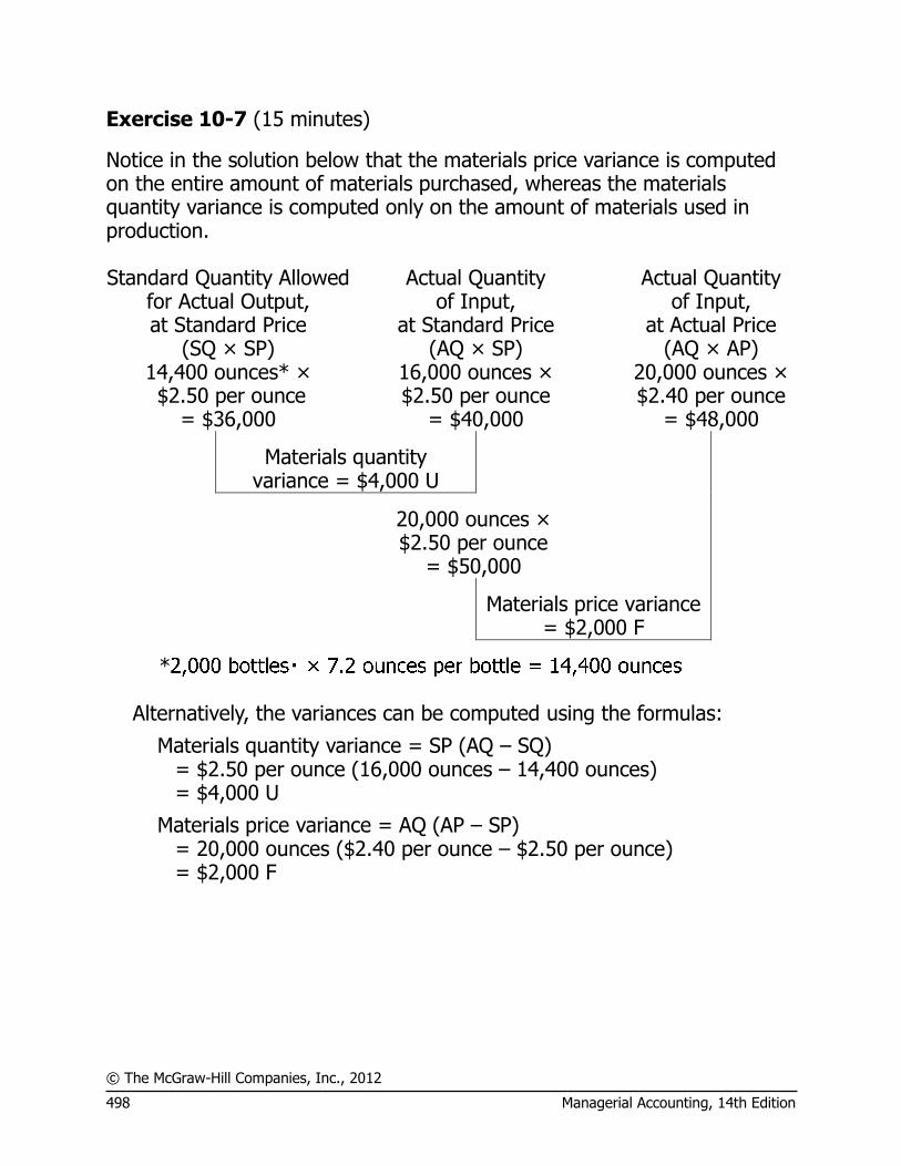
© The McGraw-Hill Companies, Inc., 2012
498 Managerial Accounting, 14th Edition
Exercise 10-7 (15 minutes)
Notice in the solution below that the materials price variance is computed on the entire amount of materials purchased, whereas the materials quantity variance is computed only on the amount of materials used in production. Standard Quantity Allowed
for Actual Output, at Standard Price
(SQ × SP)
Actual Quantity of Input,
at Standard Price (AQ × SP)
Actual Quantity of Input,
at Actual Price (AQ × AP)
14,400 ounces* × $2.50 per ounce
= $36,000
16,000 ounces × $2.50 per ounce
= $40,000
20,000 ounces × $2.40 per ounce
= $48,000
Materials quantity variance = $4,000 U
20,000 ounces × $2.50 per ounce
= $50,000
Materials price variance = $2,000 F
* Alternatively, the variances can be computed using the formulas:
Materials quantity variance = SP (AQ – SQ) = $2.50 per ounce (16,000 ounces – 14,400 ounces) = $4,000 U
Materials price variance = AQ (AP – SP) = 20,000 ounces ($2.40 per ounce – $2.50 per ounce) = $2,000 F

© The McGraw-Hill Companies, Inc., 2012. All rights reserved.
Solutions Manual, Chapter 10 499
Exercise 10-8 (30 minutes)
1. a. Notice in the solution below that the materials price variance is computed on the entire amount of materials purchased, whereas the materials quantity variance is computed only on the amount of materials used in production.
Standard Quantity Allowed
for Actual Output, at Standard Price
(SQ × SP)
Actual Quantity of Input,
at Standard Price (AQ × SP)
Actual Quantity of Input,
at Actual Price (AQ × AP)
40,000 diodes* × $0.30 per diode
= $12,000
50,000 diodes × $0.30 per diode
= $15,000
70,000 diodes × $0.28 per diode
= $19,600
Materials quantity variance = $3,000 U
70,000 diodes × $0.30 per diode
= $21,000
Materials price variance = $1,400 F
*5,000 toys × 8 diodes per toy = 40,000 diodes
Alternatively, the variances can be computed using the formulas:
Materials quantity variance = SP (AQ – SQ) = $0.30 per diode (50,000 diodes – 40,000 diodes) = $3,000 U
Materials price variance = AQ (AP – SP) = 70,000 diodes ($0.28 per diode – $0.30 per diode) = $1,400 F
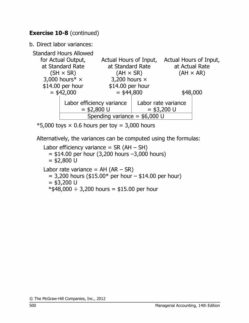
© The McGraw-Hill Companies, Inc., 2012
500 Managerial Accounting, 14th Edition
Exercise 10-8 (continued)
b. Direct labor variances:
Standard Hours Allowed for Actual Output, at Standard Rate
(SH × SR)
Actual Hours of Input, at Standard Rate
(AH × SR)
Actual Hours of Input, at Actual Rate
(AH × AR) 3,000 hours* × $14.00 per hour
= $42,000
3,200 hours × $14.00 per hour
= $44,800 $48,000
Labor efficiency variance = $2,800 U
Labor rate variance = $3,200 U
Spending variance = $6,000 U
*5,000 toys × 0.6 hours per toy = 3,000 hours Alternatively, the variances can be computed using the formulas:
Labor efficiency variance = SR (AH – SH) = $14.00 per hour (3,200 hours –3,000 hours) = $2,800 U
Labor rate variance = AH (AR – SR) = 3,200 hours ($15.00* per hour – $14.00 per hour) = $3,200 U *$48,000 ÷ 3,200 hours = $15.00 per hour

© The McGraw-Hill Companies, Inc., 2012. All rights reserved.
Solutions Manual, Chapter 10 501
Exercise 10-8 (continued)
2. A variance usually has many possible explanations. In particular, we should always keep in mind that the standards themselves may be incorrect. Some of the other possible explanations for the variances observed at Topper Toys appear below:
Materials Price Variance Since this variance is favorable, the actual price paid per unit for the material was less than the standard price. This could occur for a variety of reasons including the purchase of a lower grade material at a discount, buying in an unusually large quantity to take advantage of quantity discounts, a change in the market price of the material, and particularly sharp bargaining by the purchasing department.
Materials Quantity Variance Since this variance is unfavorable, more materials were used to produce the actual output than were called for by the standard. This could also occur for a variety of reasons. Some of the possibilities include poorly trained or supervised workers, improperly adjusted machines, and defective materials.
Labor Rate Variance Since this variance is unfavorable, the actual average wage rate was higher than the standard wage rate. Some of the possible explanations include an increase in wages that has not been reflected in the standards, unanticipated overtime, and a shift toward more highly paid workers.
Labor Efficiency Variance Since this variance is unfavorable, the actual number of labor hours was greater than the standard labor hours allowed for the actual output. As with the other variances, this variance could have been caused by any of a number of factors. Some of the possible explanations include poor supervision, poorly trained workers, low-quality materials requiring more labor time to process, and machine breakdowns. In addition, if the direct labor force is essentially fixed, an unfavorable labor efficiency variance could be caused by a reduction in output due to decreased demand for the company’s products.

© The McGraw-Hill Companies, Inc., 2012
502 Managerial Accounting, 14th Edition
Problem 10-9 (45 minutes)
1. a.
Standard Quantity Allowed for Actual Output, at Standard Price
(SQ × SP)
Actual Quantity of Input,
at Standard Price (AQ × SP)
Actual Quantity of Input,
at Actual Price (AQ × AP)
20,000 pounds* × $2.50 per pound
= $50,000
19,800 pounds × $2.50 per pound
= $49,500
25,000 pounds × $2.95 per pound
= $73,750
Materials quantity variance = $500 F
25,000 pounds × $2.50 per pound
= $62,500
Materials price variance = $11,250 U
*5,000 ingots × 4.0 pounds per ingot = 20,000 pounds Alternatively, the variances can be computed using the formulas:
Materials quantity variance = SP (AQ – SQ) = $2.50 per pound (19,800 pounds – 20,000 pounds) = $500 F
Materials price variance = AQ (AP – SP) = 25,000 pounds ($2.95 per pound – $2.50 per pound) = $11,250 U

© The McGraw-Hill Companies, Inc., 2012. All rights reserved.
Solutions Manual, Chapter 10 503
Problem 10-9 (continued)
1. b.
Standard Hours Allowed for Actual Output, at Standard Rate
(SH × SR)
Actual Hours of Input, at Standard Rate
(AH × SR)
Actual Hours of Input, at Actual Rate
(AH × AR) 3,000 hours* × $9.00 per hour
= $27,000
3,600 hours × $9.00 per hour
= $32,400
3,600 hours × $8.70 per hour
= $31,320
Labor efficiency variance = $5,400 U
Labor rate variance = $1,080 F
Spending variance = $4,320 U
*5,000 ingots × 0.6 hour per ingot = 3,000 hours Alternatively, the variances can be computed using the formulas:
Labor efficiency variance = SR (AH – SH) = $9.00 per hour (3,600 hours – 3,000 hours) = $5,400 U
Labor rate variance = AH (AR – SR) = 3,600 hours ($8.70 per hour – $9.00 per hour) = $1,080 F

© The McGraw-Hill Companies, Inc., 2012
504 Managerial Accounting, 14th Edition
Problem 10-9 (continued)
1. c.
Standard Hours Allowed for Actual Output, at Standard Rate
(SH × SR)
Actual Hours of Input, at Standard Rate
(AH × SR)
Actual Hours of Input, at Actual Rate
(AH × AR) 1,500 hours* × $2.00 per hour
= $3,000
1,800 hours × $2.00 per hour
= $3,600 $4,320
Variable overhead efficiency variance
= $600 U
Variable overhead rate variance
= $720 U
Spending variance = $1,320 U
*5,000 ingots × 0.3 hours per ingot = 1,500 hours Alternatively, the variances can be computed using the formulas:
Variable overhead efficiency variance = SR (AH – SH) = $2.00 per hour (1,800 hours – 1,500 hours) = $600 U
Variable overhead rate variance = AH (AR – SR) = 1,800 hours ($2.40 per hour* – $2.00 per hour) = $720 U *$4,320 ÷ 1,800 hours = $2.40 per hour
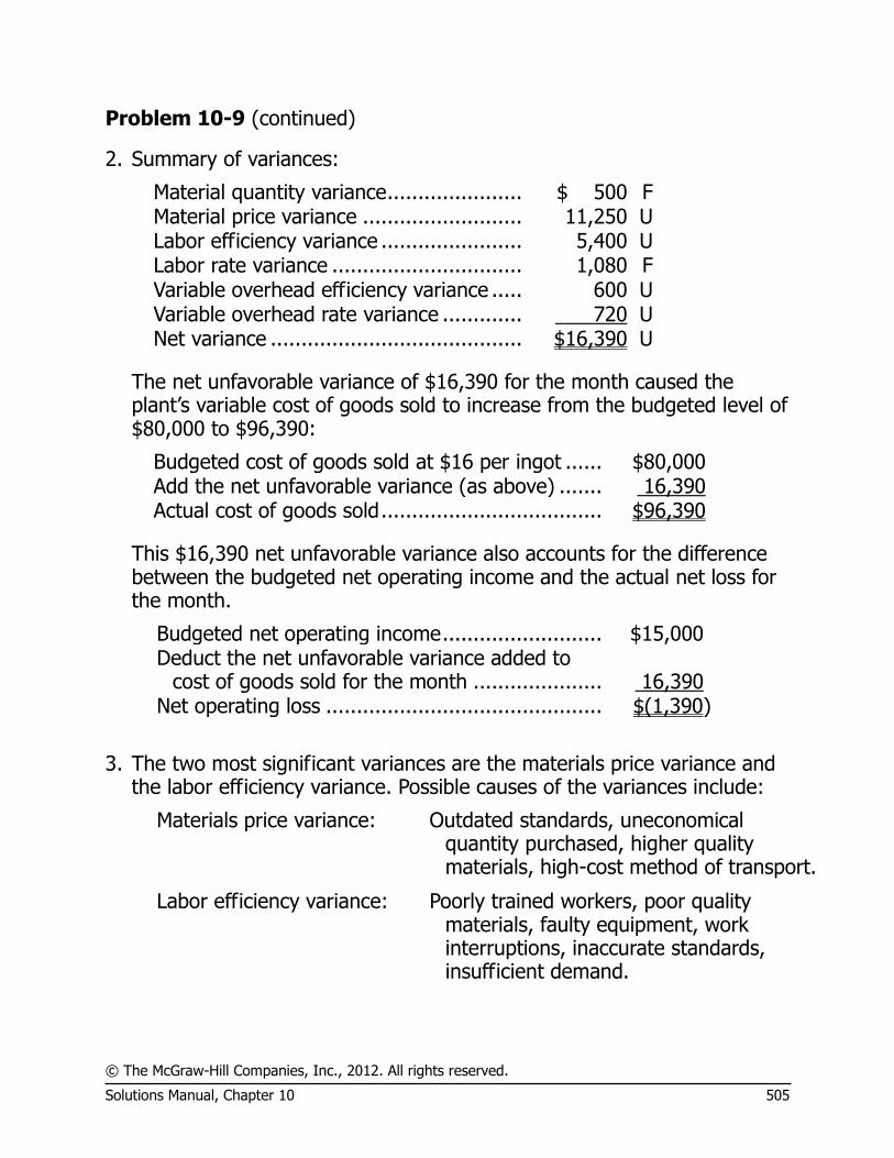
© The McGraw-Hill Companies, Inc., 2012. All rights reserved.
Solutions Manual, Chapter 10 505
Problem 10-9 (continued)
2. Summary of variances:
Material quantity variance ...................... $ 500 F Material price variance .......................... 11,250 U Labor efficiency variance ....................... 5,400 U Labor rate variance ............................... 1,080 F Variable overhead efficiency variance ..... 600 U Variable overhead rate variance ............. 720 U Net variance ......................................... $16,390 U
The net unfavorable variance of $16,390 for the month caused the plant’s variable cost of goods sold to increase from the budgeted level of $80,000 to $96,390:
Budgeted cost of goods sold at $16 per ingot ...... $80,000 Add the net unfavorable variance (as above) ....... 16,390 Actual cost of goods sold .................................... $96,390
This $16,390 net unfavorable variance also accounts for the difference between the budgeted net operating income and the actual net loss for the month.
Budgeted net operating income .......................... $15,000 Deduct the net unfavorable variance added to
cost of goods sold for the month ..................... 16,390 Net operating loss ............................................. $(1,390)
3. The two most significant variances are the materials price variance and
the labor efficiency variance. Possible causes of the variances include:
Materials price variance:
Outdated standards, uneconomical quantity purchased, higher quality materials, high-cost method of transport.
Labor efficiency variance:
Poorly trained workers, poor quality materials, faulty equipment, work interruptions, inaccurate standards, insufficient demand.

© The McGraw-Hill Companies, Inc., 2012
506 Managerial Accounting, 14th Edition
Problem 10-10 (45 minutes)
1. The standard quantity of plates allowed for tests performed during the month would be:
Smears ................................. 2,700 Blood tests ............................ 900 Total ..................................... 3,600 Plates per test ....................... × 3 Standard quantity allowed ...... 10,800
The variance analysis for plates would be:
Standard Quantity Allowed for Actual Output, at Standard Price
(SQ × SP)
Actual Quantity of Input,
at Standard Price (AQ × SP)
Actual Quantity of Input,
at Actual Price (AQ × AP)
10,800 plates × $2.50 per plate
= $27,000
14,000 plates × $2.50 per plate
= $35,000 $38,400
Materials quantity variance = $8,000 U
16,000 plates × $2.50 per plate
= $40,000
Materials price variance = $1,600 F
Alternatively, the variances can be computed using the formulas:
Materials quantity variance = SP (AQ – SQ) = $2.50 per plate (14,000 plates – 10,800 plates) = $8,000 U
s Materials price variance = AQ (AP – SP) = 16,000 plates ($2.40 per plate* – $2.50 per plate) = $1,600 F *$38,400 ÷ 16,000 plates = $2.40 per plate.

© The McGraw-Hill Companies, Inc., 2012. All rights reserved.
Solutions Manual, Chapter 10 507
Problem 10-10 (continued)
Note that all of the price variance is due to the hospital’s 4% quantity discount. Also note that the $8,000 quantity variance for the month is equal to nearly 30% of the standard cost allowed for plates. This variance may be the result of using too many assistants in the lab.
2. a. The standard hours allowed for tests performed during the month
would be:
Smears: 0.3 hour per test × 2,700 tests ..... 810 Blood tests: 0.6 hour per test × 900 tests ... 540 Total standard hours allowed ...................... 1,350
The variance analysis of labor would be:
Standard Hours Allowed for Actual Output, at Standard Rate
(SH × SR)
Actual Hours of Input, at Standard Rate
(AH × SR)
Actual Hours of Input, at Actual Rate
(AH × AR) 1,350 hours × $12 per hour = $16,200
1,800 hours × $12 per hour = $21,600 $18,450
Labor efficiency variance = $5,400 U
Labor rate variance = $3,150 F
Spending variance = $2,250 U Alternatively, the variances can be computed using the formulas:
Labor efficiency variance = SR (AH – SH) = $12 per hour (1,800 hours – 1,350 hours) = $5,400 U
Labor rate variance = AH (AR – SR) = 1,800 hours ($10.25 per hour* – $12.00 per hour) = $3,150 F *$18,450 ÷ 1,800 hours = $10.25 per hour
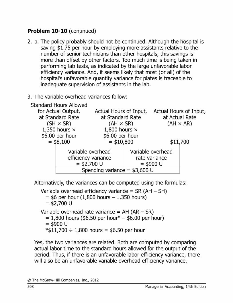
© The McGraw-Hill Companies, Inc., 2012
508 Managerial Accounting, 14th Edition
Problem 10-10 (continued)
2. b. The policy probably should not be continued. Although the hospital is saving $1.75 per hour by employing more assistants relative to the number of senior technicians than other hospitals, this savings is more than offset by other factors. Too much time is being taken in performing lab tests, as indicated by the large unfavorable labor efficiency variance. And, it seems likely that most (or all) of the hospital’s unfavorable quantity variance for plates is traceable to inadequate supervision of assistants in the lab.
3. The variable overhead variances follow:
Standard Hours Allowed for Actual Output, at Standard Rate
(SH × SR)
Actual Hours of Input, at Standard Rate
(AH × SR)
Actual Hours of Input, at Actual Rate
(AH × AR) 1,350 hours × $6.00 per hour
= $8,100
1,800 hours × $6.00 per hour
= $10,800 $11,700
Variable overhead efficiency variance
= $2,700 U
Variable overhead rate variance
= $900 U
Spending variance = $3,600 U Alternatively, the variances can be computed using the formulas:
Variable overhead efficiency variance = SR (AH – SH) = $6 per hour (1,800 hours – 1,350 hours) = $2,700 U
Variable overhead rate variance = AH (AR – SR) = 1,800 hours ($6.50 per hour* – $6.00 per hour) = $900 U *$11,700 ÷ 1,800 hours = $6.50 per hour Yes, the two variances are related. Both are computed by comparing
actual labor time to the standard hours allowed for the output of the period. Thus, if there is an unfavorable labor efficiency variance, there will also be an unfavorable variable overhead efficiency variance.
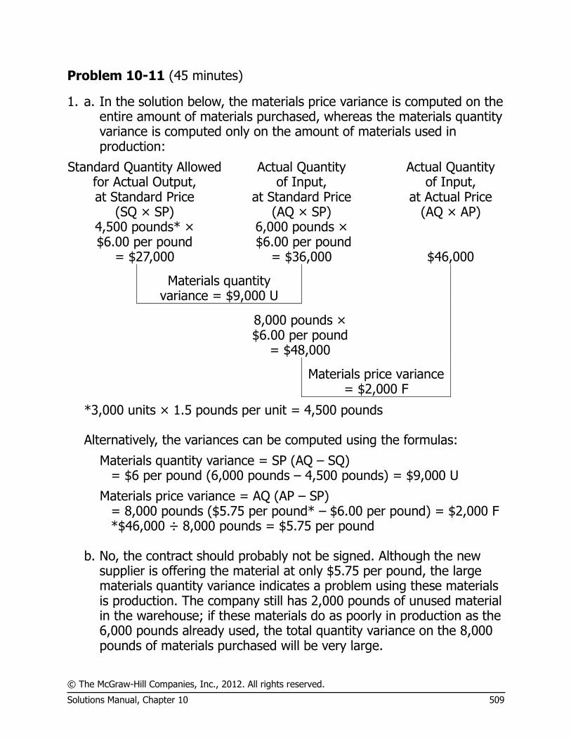
© The McGraw-Hill Companies, Inc., 2012. All rights reserved.
Solutions Manual, Chapter 10 509
Problem 10-11 (45 minutes)
1. a. In the solution below, the materials price variance is computed on the entire amount of materials purchased, whereas the materials quantity variance is computed only on the amount of materials used in production:
Standard Quantity Allowed for Actual Output, at Standard Price
(SQ × SP)
Actual Quantity of Input,
at Standard Price (AQ × SP)
Actual Quantity of Input,
at Actual Price (AQ × AP)
4,500 pounds* × $6.00 per pound
= $27,000
6,000 pounds × $6.00 per pound
= $36,000 $46,000
Materials quantity variance = $9,000 U
8,000 pounds × $6.00 per pound
= $48,000
Materials price variance = $2,000 F
*3,000 units × 1.5 pounds per unit = 4,500 pounds Alternatively, the variances can be computed using the formulas:
Materials quantity variance = SP (AQ – SQ) = $6 per pound (6,000 pounds – 4,500 pounds) = $9,000 U
Materials price variance = AQ (AP – SP) = 8,000 pounds ($5.75 per pound* – $6.00 per pound) = $2,000 F *$46,000 ÷ 8,000 pounds = $5.75 per pound b. No, the contract should probably not be signed. Although the new
supplier is offering the material at only $5.75 per pound, the large materials quantity variance indicates a problem using these materials is production. The company still has 2,000 pounds of unused material in the warehouse; if these materials do as poorly in production as the 6,000 pounds already used, the total quantity variance on the 8,000 pounds of materials purchased will be very large.
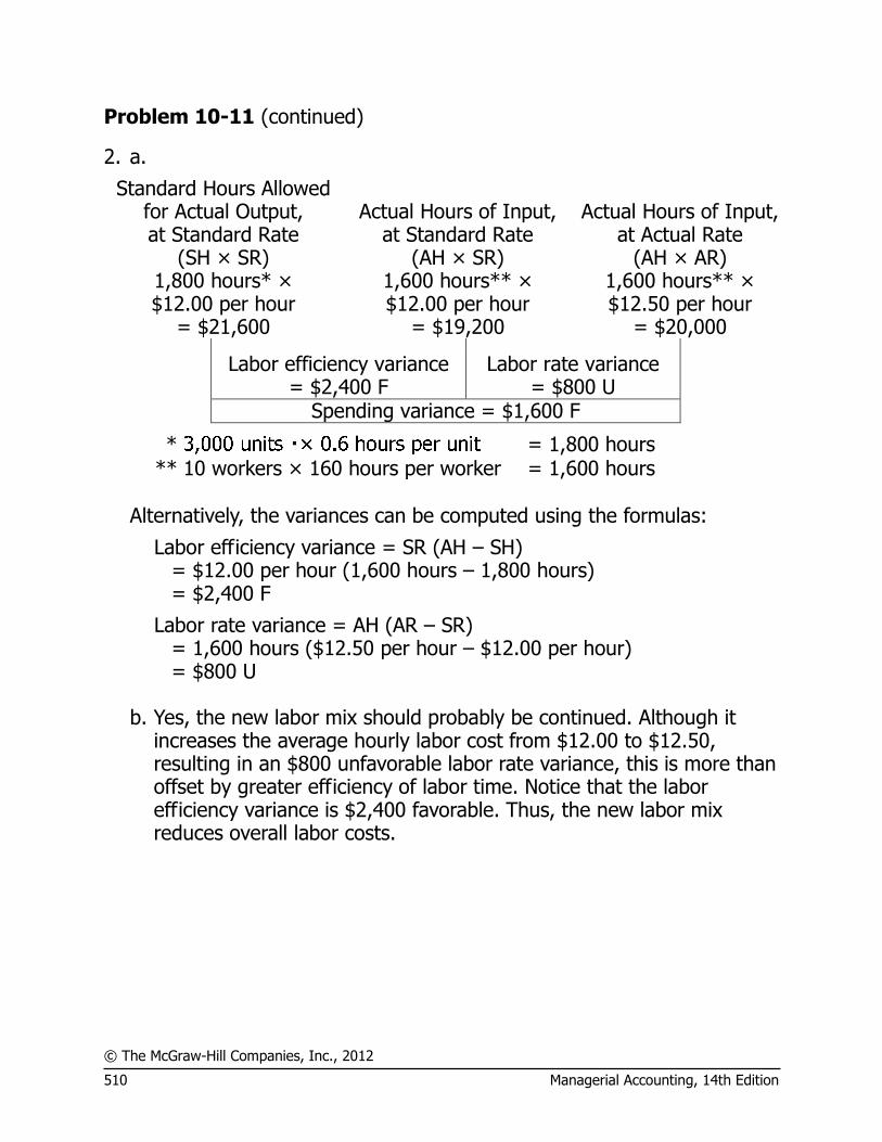
© The McGraw-Hill Companies, Inc., 2012
510 Managerial Accounting, 14th Edition
Problem 10-11 (continued)
2. a.
Standard Hours Allowed for Actual Output, at Standard Rate
(SH × SR)
Actual Hours of Input, at Standard Rate
(AH × SR)
Actual Hours of Input, at Actual Rate
(AH × AR) 1,800 hours* × $12.00 per hour
= $21,600
1,600 hours** × $12.00 per hour
= $19,200
1,600 hours** × $12.50 per hour
= $20,000
Labor efficiency variance = $2,400 F
Labor rate variance = $800 U
Spending variance = $1,600 F
* = 1,800 hours ** 10 workers × 160 hours per worker = 1,600 hours
Alternatively, the variances can be computed using the formulas:
Labor efficiency variance = SR (AH – SH) = $12.00 per hour (1,600 hours – 1,800 hours) = $2,400 F
Labor rate variance = AH (AR – SR) = 1,600 hours ($12.50 per hour – $12.00 per hour) = $800 U b. Yes, the new labor mix should probably be continued. Although it
increases the average hourly labor cost from $12.00 to $12.50, resulting in an $800 unfavorable labor rate variance, this is more than offset by greater efficiency of labor time. Notice that the labor efficiency variance is $2,400 favorable. Thus, the new labor mix reduces overall labor costs.

© The McGraw-Hill Companies, Inc., 2012. All rights reserved.
Solutions Manual, Chapter 10 511
Problem 10-11 (continued)
3.
Standard Hours Allowed for Actual Output, at Standard Rate
(SH × SR)
Actual Hours of Input, at Standard Rate
(AH × SR)
Actual Hours of Input, at Actual Rate
(AH × AR) 1,800 hours × $2.50 per hour
= $4,500
1,600 hours × $2.50 per hour
= $4,000 $3,600
Variable overhead efficiency variance
= $500 F
Variable overhead rate variance
= $400 F
Spending variance = $900 F Alternatively, the variances can be computed using the formulas:
Variable overhead efficiency variance = SR (AH – SH) = $2.50 per hour (1,600 hours – 1,800 hours) = $500 F
Variable overhead rate variance = AH (AR – SR) = 1,600 hours ($2.25 per hour* – $2.50 per hour) = $400 F *$3,600 ÷ 1,600 hours = $2.25 per hour Both the labor efficiency variance and the variable overhead efficiency
variance are computed by comparing actual labor-hours to standard labor-hours. Thus, if the labor efficiency variance is favorable, then the variable overhead efficiency variance will be favorable as well.
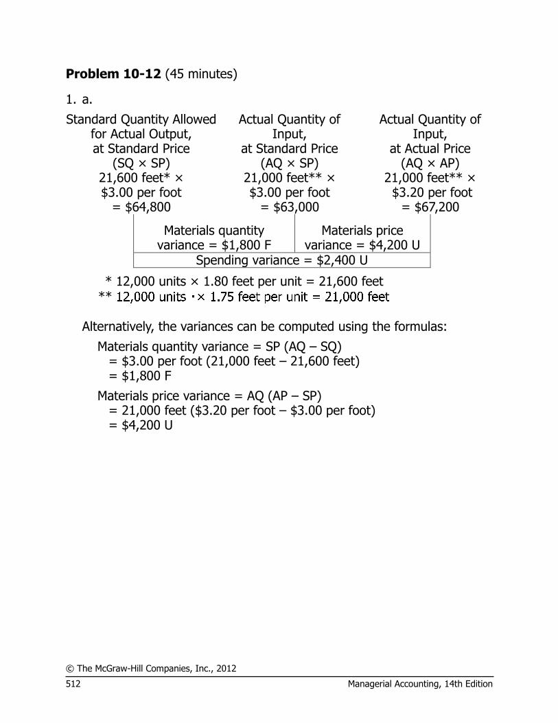
© The McGraw-Hill Companies, Inc., 2012
512 Managerial Accounting, 14th Edition
Problem 10-12 (45 minutes)
1. a.
Standard Quantity Allowed for Actual Output, at Standard Price
(SQ × SP)
Actual Quantity of Input,
at Standard Price (AQ × SP)
Actual Quantity of Input,
at Actual Price (AQ × AP)
21,600 feet* × $3.00 per foot
= $64,800
21,000 feet** × $3.00 per foot
= $63,000
21,000 feet** × $3.20 per foot
= $67,200
Materials quantity variance = $1,800 F
Materials price variance = $4,200 U
Spending variance = $2,400 U
* 12,000 units × 1.80 feet per unit = 21,600 feet **
Alternatively, the variances can be computed using the formulas:
Materials quantity variance = SP (AQ – SQ) = $3.00 per foot (21,000 feet – 21,600 feet) = $1,800 F
Materials price variance = AQ (AP – SP) = 21,000 feet ($3.20 per foot – $3.00 per foot) = $4,200 U

© The McGraw-Hill Companies, Inc., 2012. All rights reserved.
Solutions Manual, Chapter 10 513
Problem 10-12 (continued)
1. b.
Standard Hours Allowed for Actual Output, at Standard Rate
(SH × SR)
Actual Hours of Input, at Standard Rate
(AH × SR)
Actual Hours of Input, at Actual Rate
(AH × AR) 10,800 hours* × $18.00 per hour
= $194,400
11,400 hours** × $18.00 per hour
= $205,200
11,400 hours** × $17.40 per hour
= $198,360
Labor efficiency variance = $10,800 U
Labor rate variance = $6,840 F
Spending variance = $3,960 U
* 12,000 units × 0.90 hours per unit = 10,800 hours **
Alternatively, the variances can be computed using the formulas:
Labor efficiency variance = SR (AH – SH) = $18.00 per hour (11,400 hours – 10,800 hours) = $10,800 U
Labor rate variance = AH (AR – SR) = 11,400 hours ($17.40 per hour – $18.00 per hour) = $6,840 F
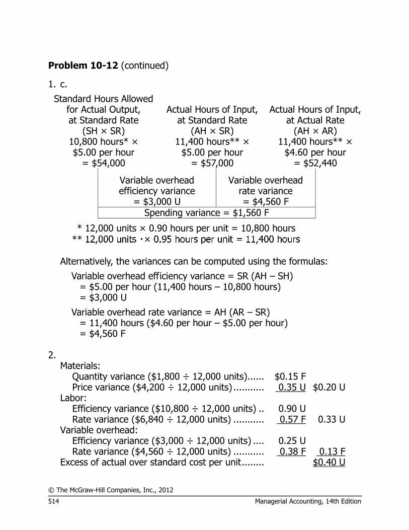
© The McGraw-Hill Companies, Inc., 2012
514 Managerial Accounting, 14th Edition
Problem 10-12 (continued)
1. c.
Standard Hours Allowed for Actual Output, at Standard Rate
(SH × SR)
Actual Hours of Input, at Standard Rate
(AH × SR)
Actual Hours of Input, at Actual Rate
(AH × AR) 10,800 hours* × $5.00 per hour
= $54,000
11,400 hours** × $5.00 per hour
= $57,000
11,400 hours** × $4.60 per hour
= $52,440
Variable overhead efficiency variance
= $3,000 U
Variable overhead rate variance = $4,560 F
Spending variance = $1,560 F
* 12,000 units × 0.90 hours per unit = 10,800 hours **
Alternatively, the variances can be computed using the formulas:
Variable overhead efficiency variance = SR (AH – SH) = $5.00 per hour (11,400 hours – 10,800 hours) = $3,000 U
Variable overhead rate variance = AH (AR – SR) = 11,400 hours ($4.60 per hour – $5.00 per hour) = $4,560 F 2.
Materials: Quantity variance ($1,800 ÷ 12,000 units) ...... $0.15 F Price variance ($4,200 ÷ 12,000 units) ........... 0.35 U $0.20 U
Labor: Efficiency variance ($10,800 ÷ 12,000 units) .. 0.90 U Rate variance ($6,840 ÷ 12,000 units) ........... 0.57 F 0.33 U
Variable overhead: Efficiency variance ($3,000 ÷ 12,000 units) .... 0.25 U Rate variance ($4,560 ÷ 12,000 units) ........... 0.38 F 0.13 F
Excess of actual over standard cost per unit ........ $0.40 U

© The McGraw-Hill Companies, Inc., 2012. All rights reserved.
Solutions Manual, Chapter 10 515
Problem 10-12 (continued)
3. Both the labor efficiency and variable overhead efficiency variances are affected by inefficient use of labor time.
Excess of actual over standard cost per unit ....... $0.40 U Less portion attributable to labor inefficiency: Labor efficiency variance ................................... 0.90 U Variable overhead efficiency variance ................. 0.25 U 1.15 U Portion due to other variances ........................... $0.75 F
In sum, had it not been for the apparent inefficient use of labor time, the total variance in unit cost for the month would have been favorable by $0.75 rather than unfavorable by $0.40.
4. Although the excess of actual cost over standard cost is only $0.40 per
unit, the total amount of $4,800 (= $0.40 per unit × 12,000 units) is substantial. Moreover, the details of the variances are significant. The materials price variance is $4,200 U, the labor efficiency variance is $10,800 U, the labor rate variance is $6,840 F, the variable overhead efficiency variance is $3,000 U, and the variable rate variance is $4,560 F. Taken together, the two variances that reflect apparent inefficient use of the labor time total $13,800 U. Each of these variances may warrant further investigation.
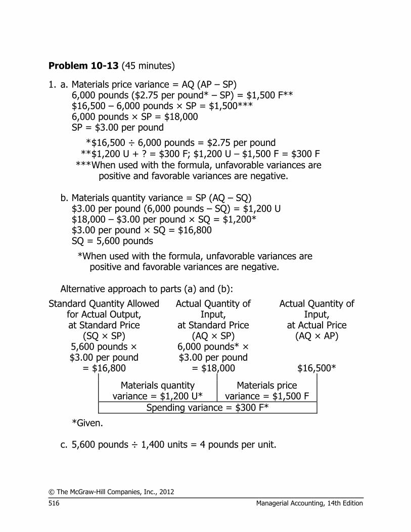
© The McGraw-Hill Companies, Inc., 2012
516 Managerial Accounting, 14th Edition
Problem 10-13 (45 minutes)
1. a. Materials price variance = AQ (AP – SP) 6,000 pounds ($2.75 per pound* – SP) = $1,500 F** $16,500 – 6,000 pounds × SP = $1,500*** 6,000 pounds × SP = $18,000 SP = $3.00 per pound
* $16,500 ÷ 6,000 pounds = $2.75 per pound ** $1,200 U + ? = $300 F; $1,200 U – $1,500 F = $300 F
*** When used with the formula, unfavorable variances are positive and favorable variances are negative.
b. Materials quantity variance = SP (AQ – SQ) $3.00 per pound (6,000 pounds – SQ) = $1,200 U $18,000 – $3.00 per pound × SQ = $1,200* $3.00 per pound × SQ = $16,800 SQ = 5,600 pounds
* When used with the formula, unfavorable variances are positive and favorable variances are negative.
Alternative approach to parts (a) and (b):
Standard Quantity Allowed for Actual Output, at Standard Price
(SQ × SP)
Actual Quantity of Input,
at Standard Price (AQ × SP)
Actual Quantity of Input,
at Actual Price (AQ × AP)
5,600 pounds × $3.00 per pound
= $16,800
6,000 pounds* × $3.00 per pound
= $18,000 $16,500*
Materials quantity variance = $1,200 U*
Materials price variance = $1,500 F
Spending variance = $300 F*
*Given. c. 5,600 pounds ÷ 1,400 units = 4 pounds per unit.
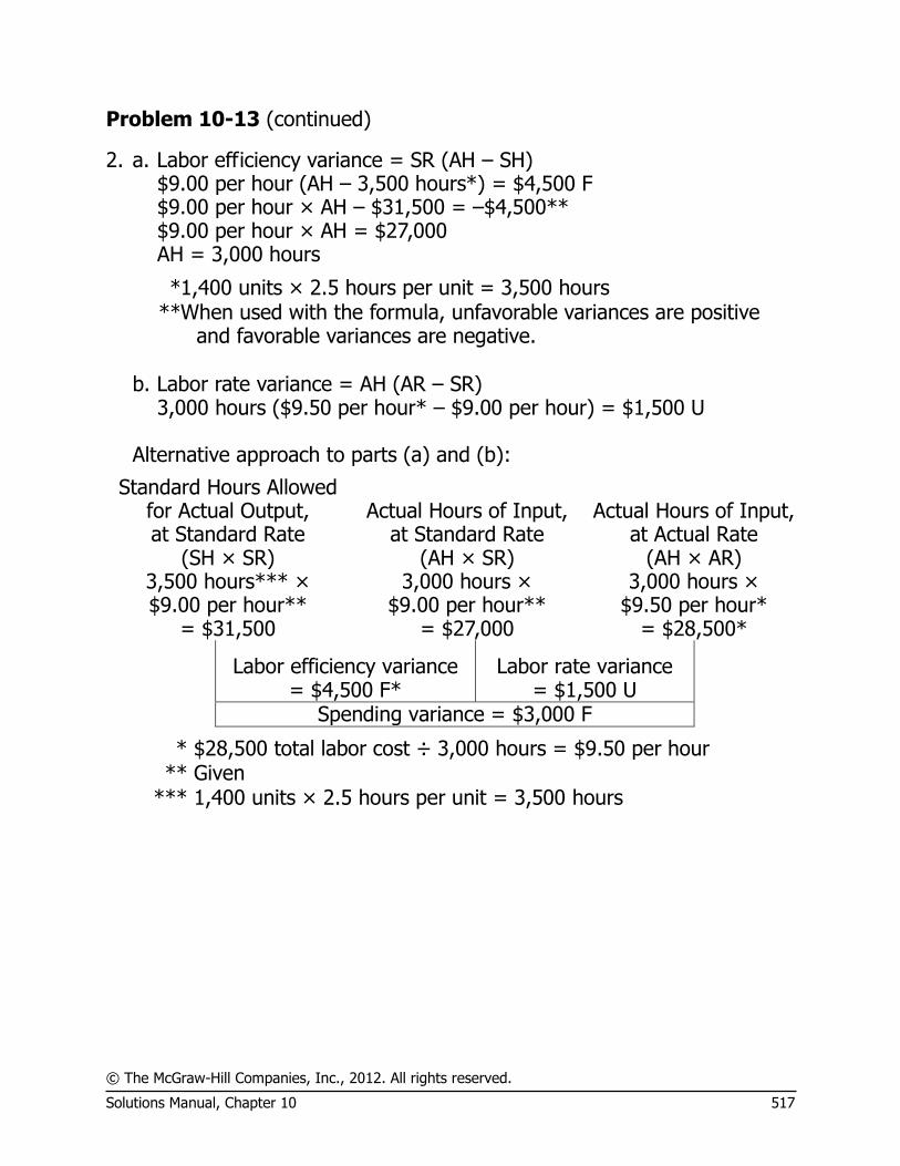
© The McGraw-Hill Companies, Inc., 2012. All rights reserved.
Solutions Manual, Chapter 10 517
Problem 10-13 (continued)
2. a. Labor efficiency variance = SR (AH – SH) $9.00 per hour (AH – 3,500 hours*) = $4,500 F $9.00 per hour × AH – $31,500 = –$4,500** $9.00 per hour × AH = $27,000 AH = 3,000 hours
* 1,400 units × 2.5 hours per unit = 3,500 hours ** When used with the formula, unfavorable variances are positive
and favorable variances are negative. b. Labor rate variance = AH (AR – SR) 3,000 hours ($9.50 per hour* – $9.00 per hour) = $1,500 U Alternative approach to parts (a) and (b):
Standard Hours Allowed for Actual Output, at Standard Rate
(SH × SR)
Actual Hours of Input, at Standard Rate
(AH × SR)
Actual Hours of Input, at Actual Rate
(AH × AR) 3,500 hours*** × $9.00 per hour**
= $31,500
3,000 hours × $9.00 per hour**
= $27,000
3,000 hours × $9.50 per hour*
= $28,500*
Labor efficiency variance = $4,500 F*
Labor rate variance = $1,500 U
Spending variance = $3,000 F
* $28,500 total labor cost ÷ 3,000 hours = $9.50 per hour ** Given *** 1,400 units × 2.5 hours per unit = 3,500 hours

© The McGraw-Hill Companies, Inc., 2012
518 Managerial Accounting, 14th Edition
Problem 10-14 (60 minutes)
1. Total standard cost for units produced during August: 500 kits × $42 per kit ........................................................ $21,000
Less standard cost of labor and overhead: Direct labor ....................................................................... (8,000) Variable manufacturing overhead ........................................ (1,600) Standard cost of materials used during August ....................... $11,400 2. Standard cost of materials used during August (a) ................. $11,400 Number of units produced (b) ............................................... 500 Standard materials cost per kit (a) ÷ (b) ................................ $22.80
Standard materials cost per kit $22.80 per kit
= =3.8 yards per kitStandard materials cost per yard $6 per yard
3. Since there were no beginning or ending inventories of materials, all of the materials that were purchased during the period were used in production. Therefore, the sum of the price and quantity variances equals the spending variance, which is the difference between the actual cost and standard cost of materials used in production.
Actual cost of material used .............. $10,000 Standard cost of material used ......... 11,400 Spending variance ............................ $ 1,400 F
As discussed above, in this case the price and quantity variances together equal the spending variance. If the quantity variance is $600 U, then the price variance must be $2,000F:
Materials price variance .................... $ 2,000 F Materials quantity variance ............... 600 U Spending variance ........................... $ 1,400 F
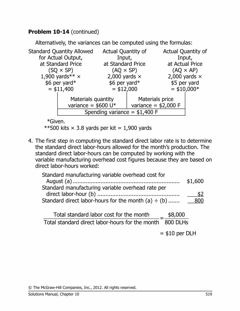
© The McGraw-Hill Companies, Inc., 2012. All rights reserved.
Solutions Manual, Chapter 10 519
Problem 10-14 (continued)
Alternatively, the variances can be computed using the formulas:
Standard Quantity Allowed for Actual Output, at Standard Price
(SQ × SP)
Actual Quantity of Input,
at Standard Price (AQ × SP)
Actual Quantity of Input,
at Actual Price (AQ × AP)
1,900 yards** × $6 per yard* = $11,400
2,000 yards × $6 per yard* = $12,000
2,000 yards × $5 per yard = $10,000*
Materials quantity variance = $600 U*
Materials price variance = $2,000 F
Spending variance = $1,400 F
* Given. ** 500 kits × 3.8 yards per kit = 1,900 yards
4. The first step in computing the standard direct labor rate is to determine
the standard direct labor-hours allowed for the month’s production. The standard direct labor-hours can be computed by working with the variable manufacturing overhead cost figures because they are based on direct labor-hours worked:
Standard manufacturing variable overhead cost for August (a) ................................................................. $1,600
Standard manufacturing variable overhead rate per direct labor-hour (b) .................................................. $2
Standard direct labor-hours for the month (a) ÷ (b) ....... 800
Total standard labor cost for the month $8,000=
Total standard direct labor-hours for the month 800 DLHs
= $10 per DLH

© The McGraw-Hill Companies, Inc., 2012
520 Managerial Accounting, 14th Edition
Problem 10-14 (continued)
5. Before the labor variances can be computed, the actual direct labor cost for the month must be computed:
Actual cost per kit produced ($42.00 + $0.14) ...... $ 42.14 Number of kits produced ..................................... × 500 Total actual cost of production ............................. $21,070 Less: Actual cost of materials ............................... $10,000
Actual cost of manufacturing variable overhead ................................................. 1,620 11,620
Actual cost of direct labor .................................... $ 9,450
With this information, the variances can be computed:
Standard Hours Allowed for Actual Output, at Standard Rate
(SH × SR)
Actual Hours of Input, at Standard Rate
(AH × SR)
Actual Hours of Input, at Actual Rate
(AH × AR)
$8,000*
900 hours* × $10 per hour
= $9,000 $9,450
Labor efficiency variance = $1,000 U
Labor rate variance = $450 U
Spending variance = $1,450 U
*Given.

© The McGraw-Hill Companies, Inc., 2012. All rights reserved.
Solutions Manual, Chapter 10 521
Problem 10-14 (continued)
6.
Standard Hours Allowed for Actual Output, at Standard Rate
(SH × SR)
Actual Hours of Input, at Standard Rate
(AH × SR)
Actual Hours of Input, at Actual Rate
(AH × AR)
$1,600*
900 hours* × $2 per hour*
= $1,800 $1,620*
Variable overhead efficiency variance
= $200 U
Variable overhead rate variance
= $180 F
Spending variance = $20 U
*Given. 7.
Standard Quantity or
Hours per Kit Standard Price
or Rate
Standard Cost per
Kit Direct materials ................. 3.8 yards1 $ 6 per yard $22.80 Direct labor ....................... 1.6 hours2 $10 per hour3 16.00
Variable manufacturing
overhead ........................ 1.6 hours $ 2 per hour 3.20 Total standard cost per kit.. $42.00
1From part 2. 2800 hours (from part 4) ÷ 500 kits = 1.6 hours per kit. 3From part 4.
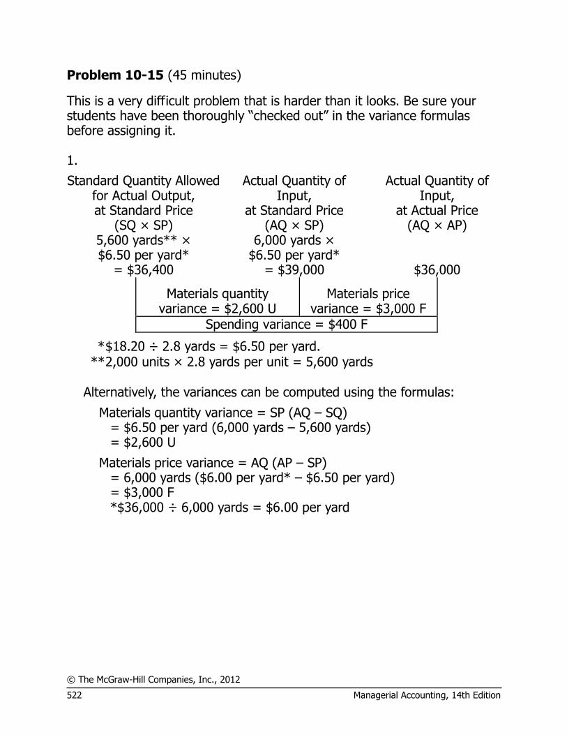
© The McGraw-Hill Companies, Inc., 2012
522 Managerial Accounting, 14th Edition
Problem 10-15 (45 minutes)
This is a very difficult problem that is harder than it looks. Be sure your students have been thoroughly “checked out” in the variance formulas before assigning it. 1.
Standard Quantity Allowed for Actual Output, at Standard Price
(SQ × SP)
Actual Quantity of Input,
at Standard Price (AQ × SP)
Actual Quantity of Input,
at Actual Price (AQ × AP)
5,600 yards** × $6.50 per yard*
= $36,400
6,000 yards × $6.50 per yard*
= $39,000 $36,000
Materials quantity variance = $2,600 U
Materials price variance = $3,000 F
Spending variance = $400 F
* $18.20 ÷ 2.8 yards = $6.50 per yard. ** 2,000 units × 2.8 yards per unit = 5,600 yards
Alternatively, the variances can be computed using the formulas:
Materials quantity variance = SP (AQ – SQ) = $6.50 per yard (6,000 yards – 5,600 yards) = $2,600 U
Materials price variance = AQ (AP – SP) = 6,000 yards ($6.00 per yard* – $6.50 per yard) = $3,000 F *$36,000 ÷ 6,000 yards = $6.00 per yard
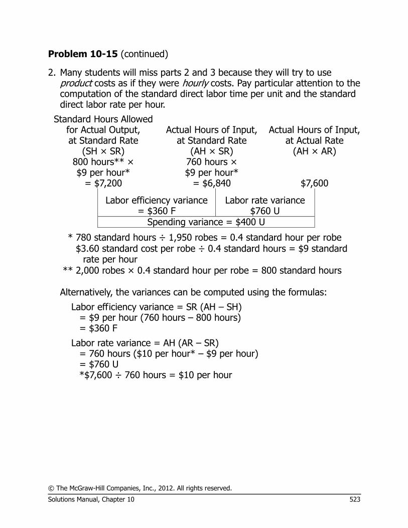
© The McGraw-Hill Companies, Inc., 2012. All rights reserved.
Solutions Manual, Chapter 10 523
Problem 10-15 (continued)
2. Many students will miss parts 2 and 3 because they will try to use product costs as if they were hourly costs. Pay particular attention to the computation of the standard direct labor time per unit and the standard direct labor rate per hour.
Standard Hours Allowed for Actual Output, at Standard Rate
(SH × SR)
Actual Hours of Input, at Standard Rate
(AH × SR)
Actual Hours of Input, at Actual Rate
(AH × AR) 800 hours** × $9 per hour*
= $7,200
760 hours × $9 per hour*
= $6,840 $7,600
Labor efficiency variance = $360 F
Labor rate variance $760 U
Spending variance = $400 U
* 780 standard hours ÷ 1,950 robes = 0.4 standard hour per robe
$3.60 standard cost per robe ÷ 0.4 standard hours = $9 standard
rate per hour ** 2,000 robes × 0.4 standard hour per robe = 800 standard hours
Alternatively, the variances can be computed using the formulas:
Labor efficiency variance = SR (AH – SH) = $9 per hour (760 hours – 800 hours) = $360 F
Labor rate variance = AH (AR – SR) = 760 hours ($10 per hour* – $9 per hour) = $760 U *$7,600 ÷ 760 hours = $10 per hour
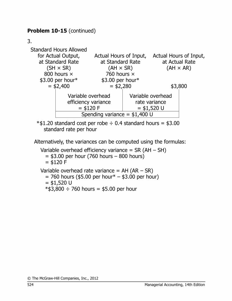
© The McGraw-Hill Companies, Inc., 2012
524 Managerial Accounting, 14th Edition
Problem 10-15 (continued)
3.
Standard Hours Allowed for Actual Output, at Standard Rate
(SH × SR)
Actual Hours of Input, at Standard Rate
(AH × SR)
Actual Hours of Input, at Actual Rate
(AH × AR) 800 hours ×
$3.00 per hour* = $2,400
760 hours × $3.00 per hour*
= $2,280 $3,800
Variable overhead efficiency variance
= $120 F
Variable overhead rate variance = $1,520 U
Spending variance = $1,400 U
* $1.20 standard cost per robe ÷ 0.4 standard hours = $3.00 standard rate per hour
Alternatively, the variances can be computed using the formulas:
Variable overhead efficiency variance = SR (AH – SH) = $3.00 per hour (760 hours – 800 hours) = $120 F
Variable overhead rate variance = AH (AR – SR) = 760 hours ($5.00 per hour* – $3.00 per hour) = $1,520 U *$3,800 ÷ 760 hours = $5.00 per hour

© The McGraw-Hill Companies, Inc., 2012. All rights reserved.
Solutions Manual, Chapter 10 525
Problem 10-16 (45 minutes)
1.
Standard Quantity or
Hours Standard Price
or Rate Standard
Cost Alpha8: Direct materials—X342 ...... 1.8 kilos $3.50 per kilo $ 6.30 Direct materials—Y561 ...... 2.0 liters $1.40 per liter 2.80 Direct labor—Sintering ....... 0.20 hours $20.00 per hour 4.00 Direct labor—Finishing ....... 0.80 hours $19.00 per hour 15.20 Total ................................ $28.30
Zeta9: Direct materials—X342 ...... 3.0 kilos $3.50 per kilo $10.50 Direct materials—Y561 ...... 4.5 liters $1.40 per liter 6.30 Direct labor—Sintering ....... 0.35 hours $20.00 per hour 7.00 Direct labor—Finishing ....... 0.90 hours $19.00 per hour 17.10 Total ................................ $40.90

© The McGraw-Hill Companies, Inc., 2012
526 Managerial Accounting, 14th Edition
Problem 10-16 (continued)
2. The computations to follow will require the standard quantities allowed for the actual output for each material.
Standard Quantity Allowed Material X342: Production of Alpha8 (1.8 kilos per unit × 1,500 units) ...... 2,700 kilos Production of Zeta9 (3.0 kilos per unit × 2,000 units) ........ 6,000 kilos Total .............................................................................. 8,700 kilos
Material Y561: Production of Alpha8 (2.0 liters per unit × 1,500 units) ..... 3,000 liters Production of Zeta9 (4.5 liters per unit × 2,000 units) ....... 9,000 liters Total .............................................................................. 12,000 liters
Direct Materials Variances—Material X342:
Materials quantity variance = SP (AQ – SQ) = $3.50 per kilo (8,500 kilos – 8,700 kilos) = $700 F
Materials price variance = AQ (AP – SP) = 14,000 kilos ($3.70 per kilo* – $3.50 per kilo) = $2,800 U *$51,800 ÷ 14,000 kilos = $3.70 per kilo Direct Materials Variances—Material Y561:
Materials quantity variance = SP (AQ – SQ) = $1.40 per liter (13,000 liters – 12,000 liters) = $1,400 U
Materials price variance = AQ (AP – SP) = 15,000 liters ($1.30 per liter* – $1.40 per liter) = $1,500 F *$19,500 ÷ 15,000 liters = $1.30 per liter

© The McGraw-Hill Companies, Inc., 2012. All rights reserved.
Solutions Manual, Chapter 10 527
Problem 10-16 (continued)
3. The computations to follow will require the standard quantities allowed for the actual output for direct labor in each department.
Standard Hours Allowed Sintering: Production of Alpha8 (0.20 hours per unit × 1,500 units) .. 300 hours Production of Zeta9 (0.35 hours per unit × 2,000 units) .... 700 hours Total .............................................................................. 1,000 hours
Finishing: Production of Alpha8 (0.80 hours per unit × 1,500 units) .. 1,200 hours Production of Zeta9 (0.90 hours per unit × 2,000 units) .... 1,800 hours Total .............................................................................. 3,000 hours
Direct Labor Variances—Sintering:
Labor efficiency variance = SR (AH – SH) = $20.00 per hour (1,200 hours – 1,000 hours) = $4,000 U
Labor rate variance = AH (AR – SR) = 1,200 hours ($22.50 per hour* – $20.00 per hour) = $3,000 U *$27,000 ÷ 1,200 hours = $22.50 per hour Direct Labor Variances—Finishing:
Labor efficiency variance = SR (AH – SH) = $19.00 per hour (2,850 hours – 3,000 hours) = $2,850 F
Labor rate variance = AH (AR – SR) = 2,850 hours ($21.00 per hour* – $19.00 per hour) = $5,700 U *$59,850 ÷ 2,850 hours = $21.00 per hour

© The McGraw-Hill Companies, Inc., 2012
528 Managerial Accounting, 14th Edition
Case 10-17 (60 minutes)
1. The number of units produced can be computed by using the total standard cost applied for the period for any input—materials, labor, or variable overhead. Using the standard cost applied for materials, we have:
Total standard cost applied $608,000
= =19,000 unitsStandard cost per unit $32.00 per unit
The same answer can be obtained by using any other cost input. 2. 40,000 meters; see the following pages for a detailed analysis. 3. $15.71 per meter; see the following pages for a detailed analysis. 4. 20,000 hours; see the following pages for a detailed analysis. 5. $15.20 per hour; see the following pages for a detailed analysis. 6. $176,000; see the following pages for a detailed analysis.
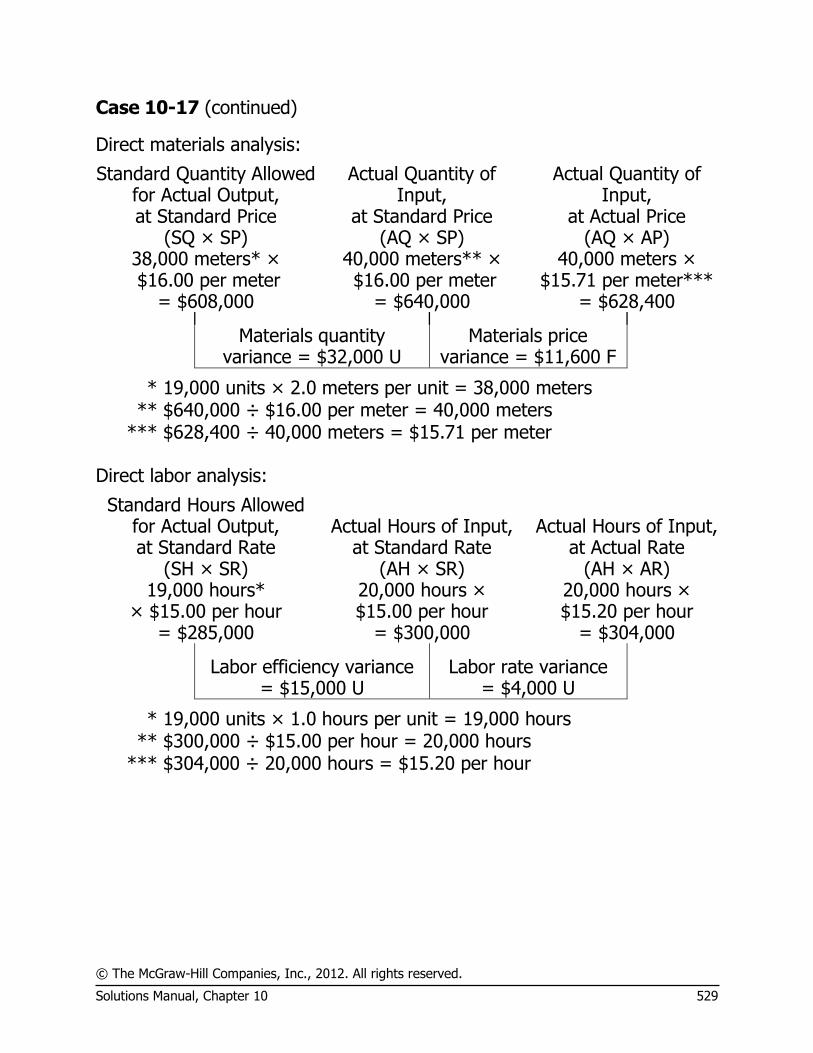
© The McGraw-Hill Companies, Inc., 2012. All rights reserved.
Solutions Manual, Chapter 10 529
Case 10-17 (continued)
Direct materials analysis:
Standard Quantity Allowed for Actual Output, at Standard Price
(SQ × SP)
Actual Quantity of Input,
at Standard Price (AQ × SP)
Actual Quantity of Input,
at Actual Price (AQ × AP)
38,000 meters* × $16.00 per meter
= $608,000
40,000 meters** × $16.00 per meter
= $640,000
40,000 meters × $15.71 per meter***
= $628,400
Materials quantity variance = $32,000 U
Materials price variance = $11,600 F
* 19,000 units × 2.0 meters per unit = 38,000 meters ** $640,000 ÷ $16.00 per meter = 40,000 meters
*** $628,400 ÷ 40,000 meters = $15.71 per meter Direct labor analysis:
Standard Hours Allowed for Actual Output, at Standard Rate
(SH × SR)
Actual Hours of Input, at Standard Rate
(AH × SR)
Actual Hours of Input, at Actual Rate
(AH × AR) 19,000 hours*
× $15.00 per hour = $285,000
20,000 hours × $15.00 per hour
= $300,000
20,000 hours × $15.20 per hour
= $304,000
Labor efficiency variance = $15,000 U
Labor rate variance = $4,000 U
* 19,000 units × 1.0 hours per unit = 19,000 hours ** $300,000 ÷ $15.00 per hour = 20,000 hours
*** $304,000 ÷ 20,000 hours = $15.20 per hour
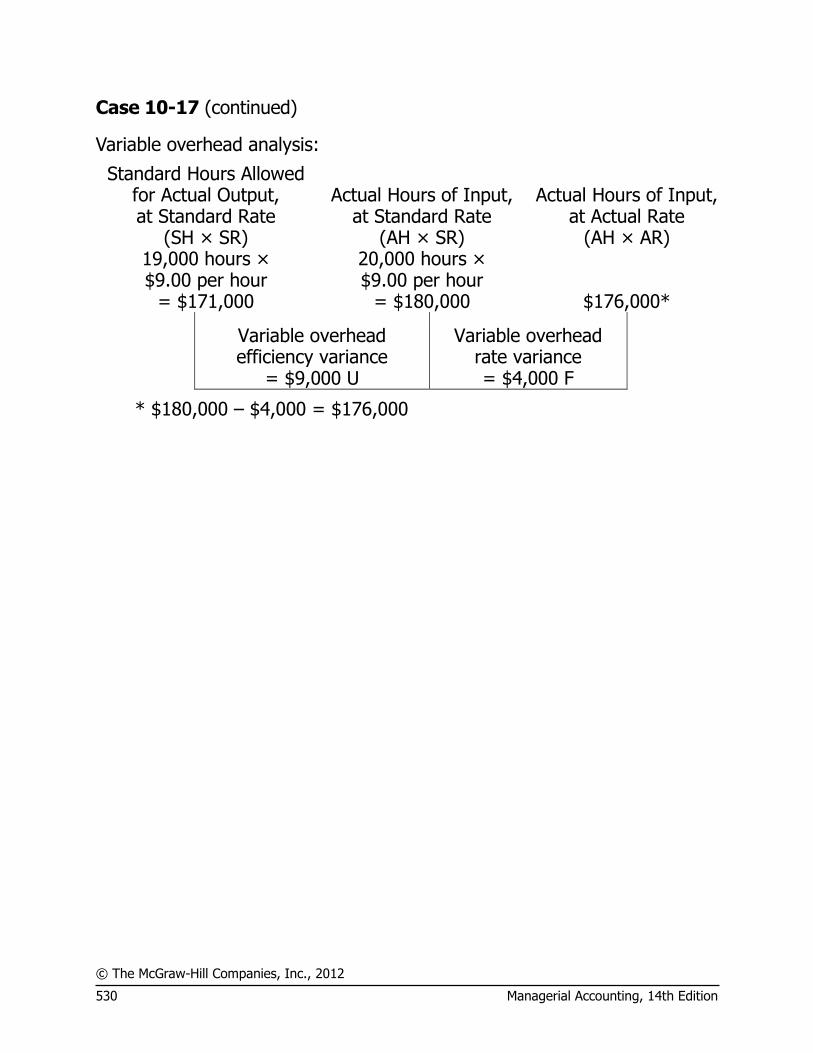
© The McGraw-Hill Companies, Inc., 2012
530 Managerial Accounting, 14th Edition
Case 10-17 (continued)
Variable overhead analysis:
Standard Hours Allowed for Actual Output, at Standard Rate
(SH × SR)
Actual Hours of Input, at Standard Rate
(AH × SR)
Actual Hours of Input, at Actual Rate
(AH × AR) 19,000 hours × $9.00 per hour
= $171,000
20,000 hours × $9.00 per hour
= $180,000 $176,000*
Variable overhead efficiency variance
= $9,000 U
Variable overhead rate variance = $4,000 F
* $180,000 – $4,000 = $176,000

© The McGraw-Hill Companies, Inc., 2012. All rights reserved.
Solutions Manual, Chapter 10 531
Appendix 10A Predetermined Overhead Rates and
Overhead Analysis in a Standard Costing System
Exercise 10A-1 (15 minutes)
1. The total overhead cost at the denominator level of activity must be determined before the predetermined overhead rate can be computed.
Total fixed overhead cost per year ................................. $600,000
Total variable overhead cost
($3.50 per DLH × 80,000 DLHs) .................................. 280,000 Total overhead cost at the denominator level of activity .. $880,000
Overhead at the denominator level of activityPredetermined=overhead rate Denominator level of activity
$880,000= =$11.00 per DLH
80,000 DLHs
2. Standard direct labor-hours allowed for
the actual output (a) ........................... 82,000 DLHs Predetermined overhead rate (b) ........... $11.00 per DLH Overhead applied (a) × (b) .................... $902,000
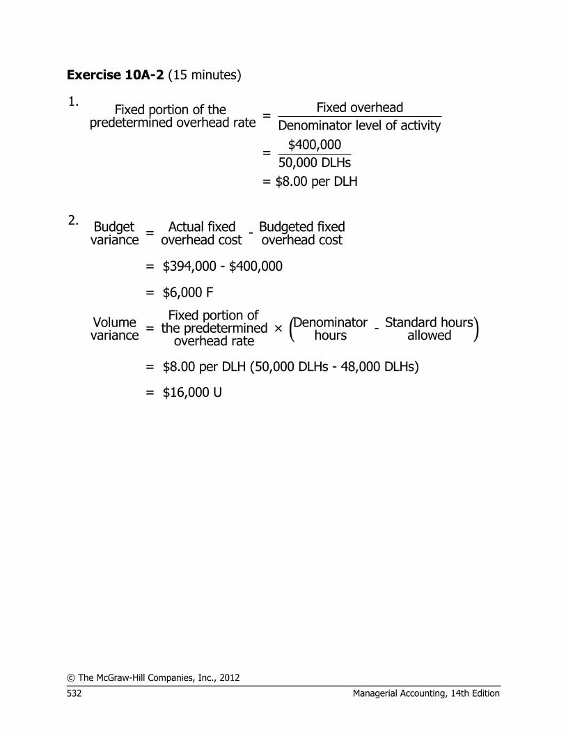
© The McGraw-Hill Companies, Inc., 2012
532 Managerial Accounting, 14th Edition
Exercise 10A-2 (15 minutes)
1. Fixed overheadFixed portion of the = predetermined overhead rate Denominator level of activity
$400,000=
50,000 DLHs
= $8.00 per DLH
2.
Budget Actual fixed Budgeted fixed = - variance overhead cost overhead cost
= $394,000 - $400,000
= $6,000 F
( )Fixed portion of
Volume Denominator Standard hours = the predetermined × - variance hours allowedoverhead rate
= $8.00 per DLH (50,000 DLHs - 48,000 DLHs)
= $16,000 U
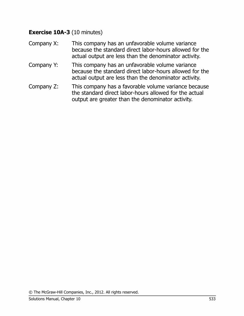
© The McGraw-Hill Companies, Inc., 2012. All rights reserved.
Solutions Manual, Chapter 10 533
Exercise 10A-3 (10 minutes)
Company X: This company has an unfavorable volume variance because the standard direct labor-hours allowed for the actual output are less than the denominator activity.
Company Y: This company has an unfavorable volume variance because the standard direct labor-hours allowed for the actual output are less than the denominator activity.
Company Z: This company has a favorable volume variance because the standard direct labor-hours allowed for the actual output are greater than the denominator activity.

© The McGraw-Hill Companies, Inc., 2012
534 Managerial Accounting, 14th Edition
Exercise 10A-4 (15 minutes)
1. Actual fixed overhead incurred ........................... $79,000 Add favorable budget variance ........................... 1,000 Budgeted fixed overhead cost ............................ $80,000
Budgeted fixed overhead cost $80,000= =$4 per MH
Denominator hours 20,000 MHs
2. 9,500 units × 2 MHs per unit = 19,000 MHs 3.
( )Fixed Portion of
Volume Denominator Standard Hours=the Predetermined - Variance Hours AllowedOverhead Rate
= $4 per MH (20,000 MHs - 19,000 MHs) = 4,000 U
Alternative solutions to parts 1-3:
Fixed Overhead Applied to Work in Process
Budgeted Fixed Overhead
Actual Fixed Overhead
19,000 MHsb × $4 per MHc = $76,000 $80,000a $79,000*
Volume variance = $4,000 U
Budget variance = $1,000 F*
*Given a$79,000 + $1,000 = $80,000 b9,500 units × 2 MHs per unit = 19,000 MHs c$80,000 ÷ 20,000 denominator MHs = $4 per MH

© The McGraw-Hill Companies, Inc., 2012. All rights reserved.
Solutions Manual, Chapter 10 535
Exercise 10A-5 (15 minutes)
1. Total overhead at thedenominator activityPredetermined =
overhead rate Denominator activity
$1.60 per DLH × 24,000 per DLH + $84,000=
24,000 DLHs
$122,400=
24,000 DLHs
= $5.10 per DLH
Variable element: ($1.60 per DLH × 24,000 DLH) ÷ 24,000 DLHs =
$38,400 ÷ 24,000 DLHs = $1.60 per DLH
Fixed element: $84,000 ÷ 24,000 DLHs = $3.50 per DLH 2. Direct materials, 2 pounds × $4.20 per pound .................... $ 8.40 Direct labor, 3 DLHs* × $12.60 per DLH ............................. 37.80 Variable manufacturing overhead, 3 DLHs × $1.60 per DLH . 4.80 Fixed manufacturing overhead, 3 DLHs × $3.50 per DLH ..... 10.50 Total standard cost per unit ............................................... $61.50
*24,000 DLHs ÷ 8,000 units = 3 DLHs per unit

© The McGraw-Hill Companies, Inc., 2012
536 Managerial Accounting, 14th Edition
Exercise 10A-6 (20 minutes)
1. $1.05 per MH × 8,000 MHs + $24,800Predetermined = overhead rate 8,000 MHs
$33,200=
8,000 MHs
= $4.15 per MH
Variable portion of $1.05 per MH × 8,000 MHsthe predetermined =
8,000 MHsoverhead rate
$8,400=
8,000 MHs
= $1.05 per MH
Fixed portion of $24,800the predetermined =
8,000 MHsoverhead rate
= $3.10 per MH
2. The standard hours per unit of product are: 8,000 MHs ÷ 3,200 units = 2.5 MHs per unit
The standard hours allowed for the actual production would be: 3,500 units × 2.5 MHs per unit = 8,750 MHs 3. Variable overhead variances: Variable overhead rate variance = (AH × AR) – (AH × SR) = ($9,860) – (8,500 MHs × $1.05 per MH) = ($9,860) – ($8,925) = $935 U
Variable overhead efficiency variance = SR (AH – SH) = $1.05 per MH (8,500 MHs – 8,750 MHs) = $262.50 F

© The McGraw-Hill Companies, Inc., 2012. All rights reserved.
Solutions Manual, Chapter 10 537
Exercise 10A-6 (continued)
Fixed overhead budget and volume variances:
Fixed Overhead Applied to Work in Process
Budgeted Fixed Overhead
Actual Fixed Overhead
8,750 standard MHs × $3.10 per MH
= $27,125 $24,800* $25,100
Volume variance = $2,325 F
Budget variance = $300 U
Total Variance = $2,025 F
*8,000 denominator MHs × $3.10 per MH = $24,800. Alternative approach to the budget variance:
Budget Actual Fixed Budgeted Fixed= - Variance Overhead Cost Overhead Cost
= $25,100 - $24,800
= $300 U
Alternative approach to the volume variance:
( )Fixed Portion of
Volume Denominator Standard Hours=the Predetermined - Variance Hours AllowedOverhead Rate
= $3.10 per MH (8,000 MHs - 8,750 MHs)
= $2,325 F

© The McGraw-Hill Companies, Inc., 2012
538 Managerial Accounting, 14th Edition
Exercise 10A-7 (15 minutes)
1. 10,000 units × 0.8 DLH per unit = 8,000 DLHs. 2. and 3.
Fixed Overhead Applied to Work in Process
Budgeted Fixed Overhead
Actual Fixed Overhead
8,000 standard DLHs × $6.00 per DLH*
= $48,000 $45,000 $45,600*
Volume variance = $3,000 F*
Budget variance = $600 U
*Given. 4. Budgeted fixed overhead costFixed cost element of the =
predetermined overhead rate Denominator activity
$45,000=
Denominator activity
=$6.00 per DLH
Therefore, the denominator activity was $45,000 ÷ $6.00 per DLH = 7,500 DLHs.

© The McGraw-Hill Companies, Inc., 2012. All rights reserved.
Solutions Manual, Chapter 10 539
Problem 10A-8 (45 minutes)
1. Direct materials price and quantity variances:
Materials quantity variance = SP (AQ – SQ) = $3.50 per yard (78,000 yards – 80,000 yards*) = $7,000 F
Materials price variance = AQ (AP – SP) = 78,000 yards ($3.75 per yard – $3.50 per yard) = $19,500 U
*20,000 units × 4 yards per unit = 80,000 yards 2. Direct labor rate and efficiency variances:
Labor efficiency variance = SR (AH – SH) = $12.00 per DLH (32,500 DLHs – 30,000 DLHs*) = $30,000 U
Labor rate variance = AH (AR – SR) = 32,500 DLHs ($11.80 per DLH – $12.00 per DLH) = $6,500 F
*20,000 units × 1.5 DLHs per unit = 30,000 DLHs 3. a. Variable manufacturing overhead spending and efficiency variances:
Standard Hours Allowed for Actual Output, at Standard Rate
(SH × SR)
Actual Hours of Input, at Standard Rate
(AH × SR)
Actual Hours of Input, at Actual Rate
(AH × AR) 30,000 DLHs ×
$2 per DLH = $60,000
32,500 DLHs × $2 per DLH = $65,000 $68,250
Variable overhead efficiency variance
= $5,000 U
Variable overhead rate variance = $3,250 U

© The McGraw-Hill Companies, Inc., 2012
540 Managerial Accounting, 14th Edition
Problem 10A-8 (continued)
Alternative solution:
Variable overhead efficiency variance = SR (AH – SH) = $2.00 per DLH (32,500 DLHs – 30,000 DLHs) = $5,000 U
Variable overhead rate variance = (AH × AR) – (AH × SR) = ($68,250) – (32,500 DLHs × $2.00 per DLH) = $3,250 U 3. b. Fixed overhead variances:
Fixed Overhead Applied to Work in Process
Budgeted Fixed Overhead
Actual Fixed Overhead
30,000 DLHs × $6 per DLH = $180,000 $150,000 $148,000
Volume variance = $30,000 F
Budget variance = $2,000 F
Alternative solution:
( )
( )
Fixed Portion ofVolume Denominator Standard Hours=the Predetermined - Variance Hours AllowedOverhead Rate
=$6.00 per DLH 25,000 DLHs – 30,000 DLHs
= $30,000 F
Budget Actual Fixed Flexible Budget Fixed= - Variance Overhead Cost Overhead Cost
=$148,000 – $150,000
=$2,000 F

© The McGraw-Hill Companies, Inc., 2012. All rights reserved.
Solutions Manual, Chapter 10 541
Problem 10A-8 (continued)
4. The total of the variances would be:
Direct materials variances: Quantity variance .......................................... $ 7,000 F Price variance ............................................... 19,500 U
Direct labor variances: Efficiency variance ........................................ 30,000 U Rate variance................................................ 6,500 F
Variable manufacturing overhead variances: Efficiency variance ........................................ 5,000 U Rate variance................................................ 3,250 U
Fixed manufacturing overhead variances: Volume variance ........................................... 30,000 F Budget variance ............................................ 2,000 F
Total of variances ............................................ $12,250 U
Notice that the total of the variances agrees with the $12,250 unfavorable variance mentioned by the vice president.
It appears that not everyone should be given a bonus for good cost control. The materials price variance and the labor efficiency variance are 7.1% and 8.3%, respectively, of the standard cost allowed and thus would warrant investigation. In addition, the variable overhead spending variance is 5.0% of the standard cost allowed.
The reason the company’s large unfavorable variances (for materials price and labor efficiency) do not show up more clearly is that they are offset by the company’s favorable volume variance for the year. This favorable volume variance is the result of the company operating at an activity level that is well above the denominator activity level used to set predetermined overhead rates. (The company operated at an activity level of 30,000 standard DLHs; the denominator activity level set at the beginning of the year was 25,000 DLHs.) As a result of the large favorable volume variance, the unfavorable price and efficiency variances have been concealed in a small “net” figure. Finally, the large favorable volume variance may have been achieved by building up inventories.

© The McGraw-Hill Companies, Inc., 2012
542 Managerial Accounting, 14th Edition
Problem 10A-9 (60 minutes)
1. and 2. Per Direct Labor-Hour Variable Fixed Total Denominator of 40,000 DLHs: $2.50 $ 2.50 $8.00 8.00 Total predetermined rate .................... $10.50 Denominator of 50,000 DLHs: $2.50 $ 2.50 $6.40 6.40 Total predetermined rate .................... $ 8.90
3. Denominator Activity:
40,000 DLHs Denominator Activity:
50,000 DLHs Direct materials, 3 yards
× $5.00 per yard .......... $15.00 Same .............................. $15.00 Direct labor, 2.5 DLHs ×
$20.00 per DLH ............ 50.00 Same .............................. 50.00 Variable overhead, 2.5
DLHs × $2.50 per DLH .. 6.25 Same .............................. 6.25 Fixed overhead, 2.5 DLHs
× $8.00 per DLH .......... 20.00 Fixed overhead, 2.5 DLHs
× $6.40 per DLH ........... 16.00 Total standard cost per
unit .............................. $91.25 Total standard cost per
unit .............................. $87.25
4. a. 18,500 units × 2.5 DLHs per unit = 46,250 standard DLHs b. Manufacturing Overhead Actual costs 446,500 Applied costs (46,250
standard DLHs* × $10.50 per DLH) 485,625
Overapplied overhead 39,125
*Determined in (a).

© The McGraw-Hill Companies, Inc., 2012. All rights reserved.
Solutions Manual, Chapter 10 543
Problem 10A-9 (continued)
4. c. Standard Hours Allowed
for Actual Output, at Standard Rate
(SH × SR)
Actual Hours of Input, at Standard Rate
(AH × SR)
Actual Hours of Input, at Actual Rate
(AH × AR) 46,250 DLHs × $2.50 per DLH = $115,625
48,000 DLHs × $2.50 per DLH = $120,000 $124,800
Variable overhead efficiency variance
= $4,375 U
Variable overhead rate variance = $4,800 U
Alternative solution: Variable overhead efficiency variance = SR (AH – SH) = $2.50 per DLH (48,000 DLHs – 46,250 DLHs) = $4,375 U
Variable overhead rate variance = (AH × AR) – (AH × SR) = ($124,800) – (48,000 DLHs × $2.50 per DLH) = $4,800 U Fixed overhead variances:
Fixed Overhead Applied to Work in Process
Budgeted Fixed Overhead
Actual Fixed Overhead
46,250 standard DLHs × $8.00 per DLH
= $370,000 $320,000* $321,700
Volume variance = $50,000 F
Budget variance = $1,700 U
*40,000 denominator DLHs × $8 per DLH = $320,000.

© The McGraw-Hill Companies, Inc., 2012
544 Managerial Accounting, 14th Edition
Problem 10A-9 (continued)
Alternative solution:
Budget Actual Fixed Flexible Budget Fixed = - Variance Overhead Cost Overhead Cost
= $321,700 – $320,000
= $1,700 U
( )
( )
Fixed Portion ofVolume Denominator Standard Hours = the Predetermined × - Variance Hours AllowedOverhead Rate
= $8.00 per DLH 40,000 DLHs – 46,250 DLHs
= $50,000 F
Summary of variances:
Variable overhead efficiency ...... $ 4,375 U Variable overhead rate variance . 4,800 U Fixed overhead volume ............. 50,000 F Fixed overhead budget .............. 1,700 U Overapplied overhead ............... $39,125 F

© The McGraw-Hill Companies, Inc., 2012. All rights reserved.
Solutions Manual, Chapter 10 545
Problem 10A-9 (continued)
5. The major disadvantage of using normal activity as the denominator in the predetermined rate is the large volume variance that ordinarily results. This occurs because the denominator activity used to compute the predetermined overhead rate is different from the activity level that is anticipated for the period. In the case at hand, the company has used the normal activity of 40,000 direct labor-hours to compute the predetermined overhead rate, whereas activity for the period was expected to be 50,000 DLHs. This has resulted in a large favorable volume variance that may be difficult for management to interpret. In addition, the large favorable volume variance in this case has masked the fact that the company did not achieve the budgeted level of activity for the period. The company had planned to work 50,000 DLHs, but managed to work only 46,250 DLHs (at standard). This unfavorable result is concealed due to using a denominator figure that is out of step with current activity.
On the other hand, by using normal activity as the denominator unit costs are stable from year to year. Thus, management’s decisions are not clouded by unit costs that jump up and down as the activity level rises and falls.

© The McGraw-Hill Companies, Inc., 2012
546 Managerial Accounting, 14th Edition
Problem 10A-10 (45 minutes)
1. £31,500 + £72,000Total rate: =£5.75 per MH
18,000 MHs
£31,500Variable element: =£1.75 per MH
18,000 MHs
£72,000Fixed element: =£4.00 per MH
18,000 MHs
2. 16,000 standard MHs × £5.75 per MH = £92,000 3. Variable manufacturing overhead variances:
Standard Hours Allowed for Actual Output, at Standard Rate
(SH × SR)
Actual Hours of Input, at Standard Rate
(AH × SR)
Actual Hours of Input, at Actual Rate
(AH × AR) 16,000 MHs × £1.75 per MH
= £28,000
15,000 MHs × £1.75 per MH
= £26,250 £26,500
Variable overhead efficiency variance
= £1,750 F
Variable overhead rate variance
= £250 U
Alternative solution:
Variable overhead efficiency variance = SR (AH – SH) = £1.75 per MH (15,000 MHs – 16,000 MHs) = £1,750 F
Variable overhead rate variance = (AH × AR) – (AH × SR) = (£26,500) – (15,000 MHs × £1.75 per MH) = £250 U

© The McGraw-Hill Companies, Inc., 2012. All rights reserved.
Solutions Manual, Chapter 10 547
Problem 10A-10 (continued)
Fixed overhead variances:
Fixed Overhead Applied to Work in Process
Budgeted Fixed Overhead
Actual Fixed Overhead
16,000 MHs × £4 per MH = £64,000 £72,000 £70,000
Volume variance = £8,000 U
Budget variance = £2,000 F
Alternative solution:
( )
( )
Fixed Portion ofVolume Denominator Standard Hours = the Predetermined - Variance Hours AllowedOverhead Rate
= £4 per MH 18,000 MHs – 16,000 MHs
= £8,000 U
Budget Actual Fixed Flexible Budget Fixed = - Variance Overhead Cost Overhead Cost
= £70,000 – £72,000
= £2,000 F
Verification of variances:
Variable overhead efficiency variance ............... £1,750 F Variable overhead rate variance ....................... 250 U Fixed overhead volume variance ...................... 8,000 U Fixed overhead budget variance ....................... 2,000 F Underapplied overhead ................................... £4,500 U

© The McGraw-Hill Companies, Inc., 2012
548 Managerial Accounting, 14th Edition
Problem 10A-10 (continued)
4. Variable overhead
Variable overhead rate variance: This variance includes both price and quantity elements. The overhead spending variance reflects differences between actual and standard prices for variable overhead items. It also reflects differences between the amounts of variable overhead inputs that were actually used and the amounts that should have been used for the actual output of the period. Because the variable overhead spending variance is unfavorable, either too much was paid for variable overhead items or too many of them were used.
Variable overhead efficiency variance: The term “variable overhead efficiency variance” is a misnomer, because the variance does not measure efficiency in the use of overhead items. It measures the indirect effect on variable overhead of the efficiency or inefficiency with which the activity base is utilized. In this company, machine-hours is the activity base. If variable overhead is really proportional to machine-hours, then more effective use of machine-hours has the indirect effect of reducing variable overhead. Because 1,000 fewer machine-hours were required than indicated by the standards, the indirect effect was presumably to reduce variable overhead spending by about £1,750 (£1.75 per machine-hour × 1,000 machine-hours).
Fixed overhead
Fixed overhead budget variance: This variance is simply the difference between the budgeted fixed cost and the actual fixed cost. In this case, the variance is favorable, which indicates that actual fixed costs were lower than anticipated in the budget.
Fixed overhead volume variance: This variance occurs as a result of actual activity being different from the denominator activity that was used in the predetermined overhead rate. In this case, the variance is unfavorable, so actual activity was less than the denominator activity. It is difficult to place much of a meaningful economic interpretation on this variance. It tends to be large, so it often swamps the other, more meaningful variances if they are simply netted against each other.
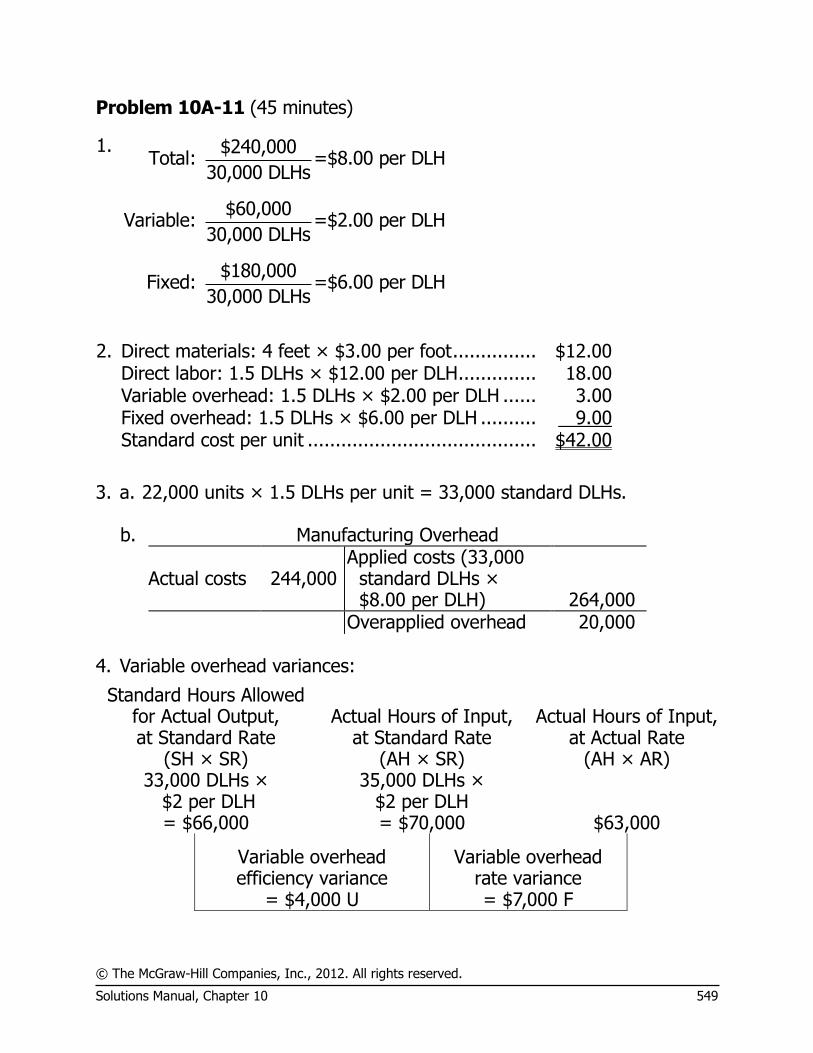
© The McGraw-Hill Companies, Inc., 2012. All rights reserved.
Solutions Manual, Chapter 10 549
Problem 10A-11 (45 minutes)
1. $240,000Total: =$8.00 per DLH
30,000 DLHs
$60,000Variable: =$2.00 per DLH
30,000 DLHs
$180,000Fixed: =$6.00 per DLH
30,000 DLHs
2. Direct materials: 4 feet × $3.00 per foot ............... $12.00 Direct labor: 1.5 DLHs × $12.00 per DLH .............. 18.00 Variable overhead: 1.5 DLHs × $2.00 per DLH ...... 3.00 Fixed overhead: 1.5 DLHs × $6.00 per DLH .......... 9.00 Standard cost per unit ......................................... $42.00
3. a. 22,000 units × 1.5 DLHs per unit = 33,000 standard DLHs.
b. Manufacturing Overhead
Actual costs 244,000
Applied costs (33,000 standard DLHs × $8.00 per DLH)
264,000
Overapplied overhead 20,000 4. Variable overhead variances:
Standard Hours Allowed for Actual Output, at Standard Rate
(SH × SR)
Actual Hours of Input, at Standard Rate
(AH × SR)
Actual Hours of Input, at Actual Rate
(AH × AR) 33,000 DLHs ×
$2 per DLH = $66,000
35,000 DLHs × $2 per DLH = $70,000 $63,000
Variable overhead efficiency variance
= $4,000 U
Variable overhead rate variance = $7,000 F
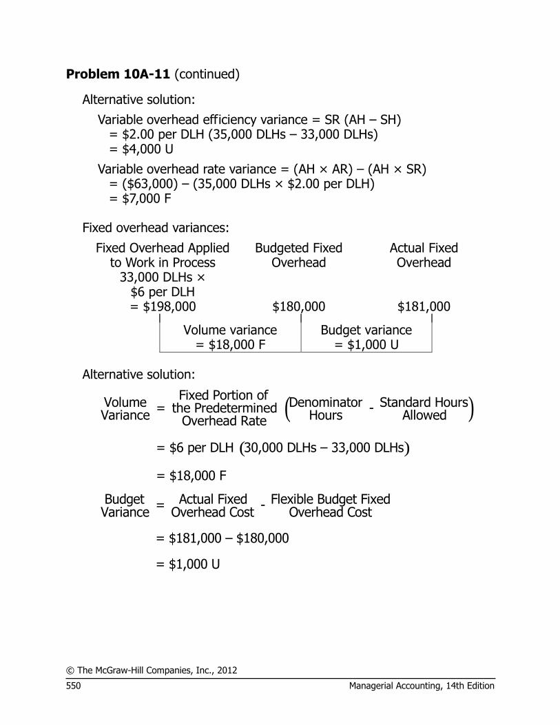
© The McGraw-Hill Companies, Inc., 2012
550 Managerial Accounting, 14th Edition
Problem 10A-11 (continued)
Alternative solution:
Variable overhead efficiency variance = SR (AH – SH) = $2.00 per DLH (35,000 DLHs – 33,000 DLHs) = $4,000 U
Variable overhead rate variance = (AH × AR) – (AH × SR) = ($63,000) – (35,000 DLHs × $2.00 per DLH) = $7,000 F Fixed overhead variances:
Fixed Overhead Applied to Work in Process
Budgeted Fixed Overhead
Actual Fixed Overhead
33,000 DLHs × $6 per DLH = $198,000 $180,000 $181,000
Volume variance = $18,000 F
Budget variance = $1,000 U
Alternative solution:
( )
( )
Fixed Portion ofVolume Denominator Standard Hours = the Predetermined - Variance Hours AllowedOverhead Rate
= $6 per DLH 30,000 DLHs – 33,000 DLHs
= $18,000 F
Budget Actual Fixed Flexible Budget Fixed = - Variance Overhead Cost Overhead Cost
= $181,000 – $180,000
= $1,000 U

© The McGraw-Hill Companies, Inc., 2012. All rights reserved.
Solutions Manual, Chapter 10 551
Problem 10A-11 (continued)
Summary of variances: Variable overhead efficiency variance ................. $ 4,000 U Variable overhead rate variance ......................... 7,000 F Fixed overhead volume variance ........................ 18,000 F Fixed overhead budget variance ......................... 1,000 U Overapplied overhead—see part 3...................... $20,000 F
5. Only the volume variance would have changed. It would have been
unfavorable, because the standard DLHs allowed for the year’s production (33,000 DLHs) would have been less than the denominator DLHs (36,000 DLHs).
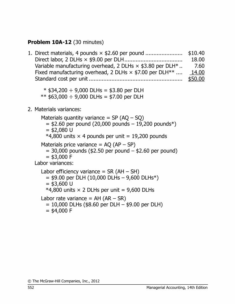
© The McGraw-Hill Companies, Inc., 2012
552 Managerial Accounting, 14th Edition
Problem 10A-12 (30 minutes)
1. Direct materials, 4 pounds × $2.60 per pound ....................... $10.40 Direct labor, 2 DLHs × $9.00 per DLH .................................... 18.00 Variable manufacturing overhead, 2 DLHs × $3.80 per DLH* .. 7.60 Fixed manufacturing overhead, 2 DLHs × $7.00 per DLH** .... 14.00 Standard cost per unit .......................................................... $50.00
* $34,200 ÷ 9,000 DLHs = $3.80 per DLH ** $63,000 ÷ 9,000 DLHs = $7.00 per DLH
2. Materials variances:
Materials quantity variance = SP (AQ – SQ) = $2.60 per pound (20,000 pounds – 19,200 pounds*) = $2,080 U *4,800 units × 4 pounds per unit = 19,200 pounds
Materials price variance = AQ (AP – SP) = 30,000 pounds ($2.50 per pound – $2.60 per pound) = $3,000 F Labor variances:
Labor efficiency variance = SR (AH – SH) = $9.00 per DLH (10,000 DLHs – 9,600 DLHs*) = $3,600 U *4,800 units × 2 DLHs per unit = 9,600 DLHs
Labor rate variance = AH (AR – SR) = 10,000 DLHs ($8.60 per DLH – $9.00 per DLH) = $4,000 F
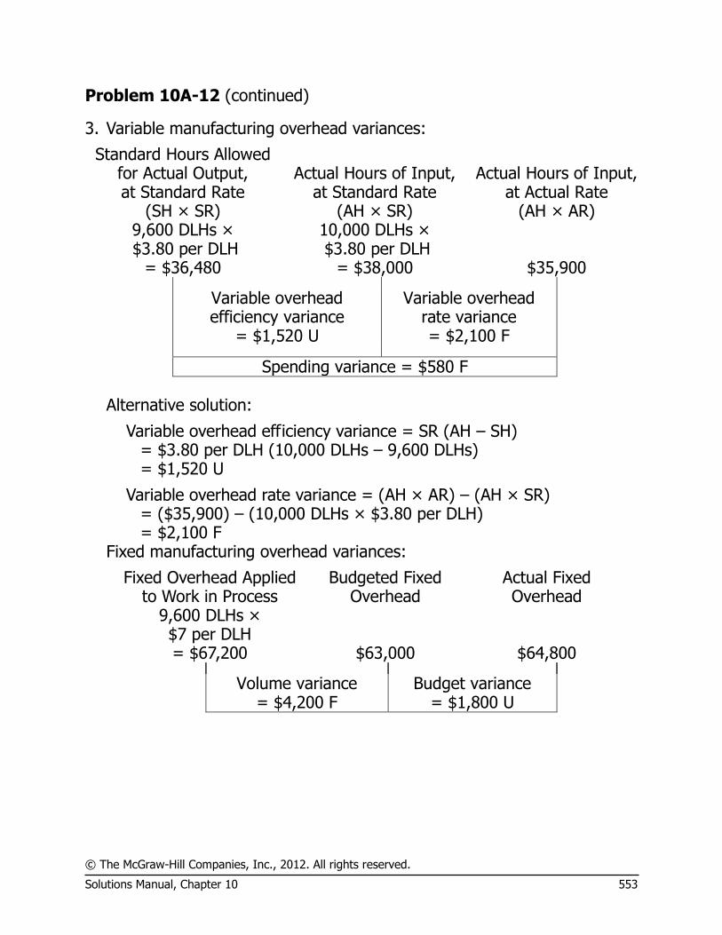
© The McGraw-Hill Companies, Inc., 2012. All rights reserved.
Solutions Manual, Chapter 10 553
Problem 10A-12 (continued)
3. Variable manufacturing overhead variances:
Standard Hours Allowed for Actual Output, at Standard Rate
(SH × SR)
Actual Hours of Input, at Standard Rate
(AH × SR)
Actual Hours of Input, at Actual Rate
(AH × AR) 9,600 DLHs × $3.80 per DLH
= $36,480
10,000 DLHs × $3.80 per DLH
= $38,000 $35,900
Variable overhead efficiency variance
= $1,520 U
Variable overhead rate variance = $2,100 F
Spending variance = $580 F Alternative solution:
Variable overhead efficiency variance = SR (AH – SH) = $3.80 per DLH (10,000 DLHs – 9,600 DLHs) = $1,520 U
Variable overhead rate variance = (AH × AR) – (AH × SR) = ($35,900) – (10,000 DLHs × $3.80 per DLH) = $2,100 F Fixed manufacturing overhead variances:
Fixed Overhead Applied to Work in Process
Budgeted Fixed Overhead
Actual Fixed Overhead
9,600 DLHs × $7 per DLH = $67,200 $63,000 $64,800
Volume variance = $4,200 F
Budget variance = $1,800 U

© The McGraw-Hill Companies, Inc., 2012
554 Managerial Accounting, 14th Edition
Problem 10A-12 (continued)
Alternative solution:
( )
( )
Fixed Portion ofVolume Denominator Standard Hours = the Predetermined - Variance Hours AllowedOverhead Rate
= $7 per DLH 9,000 DLHs – 9,600 DLHs
= $4,200 F
Budget Actual Fixed Budgeted Fixed = - Variance Overhead Cost Overhead Cost
= $64,800 – $63,000
= $1,800 U
4. The choice of a denominator activity level affects standard unit costs in
that the higher the denominator activity level chosen, the lower standard unit costs will be. The reason is that the fixed portion of overhead costs is spread over more units as the denominator activity increases.
The volume variance cannot be controlled by controlling spending. The volume variance simply reflects whether actual activity was greater or less than the denominator activity. Thus, the volume variance is controllable only through activity.

© The McGraw-Hill Companies, Inc., 2012. All rights reserved.
Solutions Manual, Chapter 10 555
Appendix 10B Journal Entries to Record Variances
Exercise 10B-1 (20 minutes)
1. The general ledger entry to record the purchase of materials for the month is:
Raw Materials
(15,000 meters at $5.40 per meter) .................. 81,000
Materials Price Variance
(15,000 meters at $0.20 per meter U) ............... 3,000
Accounts Payable
(15,000 meters at $5.60 per meter) ............. 84,000 2. The general ledger entry to record the use of materials for the month is:
Work in Process
(12,000 meters at $5.40 per meter) .................. 64,800
Materials Quantity Variance
(100 meters at $5.40 per meter F) ............... 540
Raw Materials
(11,900 meters at $5.40 per meter) ............. 64,260 3. The general ledger entry to record the incurrence of direct labor cost for
the month is:
Work in Process (2,000 hours at $14.00 per hour) 28,000
Labor Rate Variance
(1,950 hours at $0.20 per hour U) ..................... 390
Labor Efficiency Variance
(50 hours at $14.00 per hour F) ................... 700
Wages Payable
(1,950 hours at $14.20 per hour) ................. 27,690
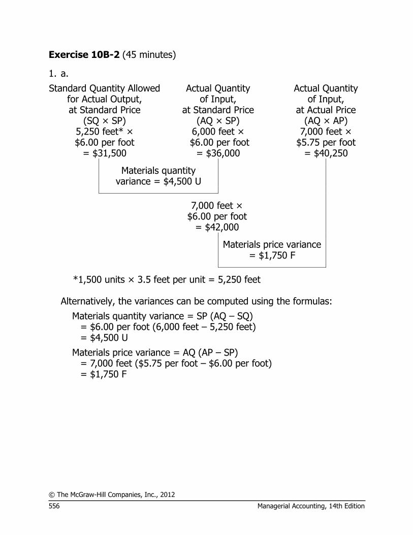
© The McGraw-Hill Companies, Inc., 2012
556 Managerial Accounting, 14th Edition
Exercise 10B-2 (45 minutes)
1. a.
Standard Quantity Allowed for Actual Output, at Standard Price
(SQ × SP)
Actual Quantity of Input,
at Standard Price (AQ × SP)
Actual Quantity of Input,
at Actual Price (AQ × AP)
5,250 feet* × $6.00 per foot
= $31,500
6,000 feet × $6.00 per foot
= $36,000
7,000 feet × $5.75 per foot
= $40,250
Materials quantity variance = $4,500 U
7,000 feet × $6.00 per foot
= $42,000
Materials price variance = $1,750 F
*1,500 units × 3.5 feet per unit = 5,250 feet Alternatively, the variances can be computed using the formulas:
Materials quantity variance = SP (AQ – SQ) = $6.00 per foot (6,000 feet – 5,250 feet) = $4,500 U
Materials price variance = AQ (AP – SP) = 7,000 feet ($5.75 per foot – $6.00 per foot) = $1,750 F
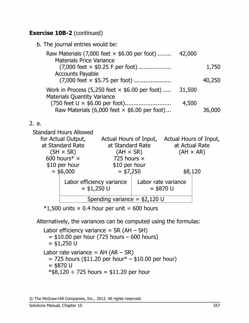
© The McGraw-Hill Companies, Inc., 2012. All rights reserved.
Solutions Manual, Chapter 10 557
Exercise 10B-2 (continued)
b. The journal entries would be:
Raw Materials (7,000 feet × $6.00 per foot) ........ 42,000 Materials Price Variance
(7,000 feet × $0.25 F per foot) ................... 1,750 Accounts Payable
(7,000 feet × $5.75 per foot) ...................... 40,250
Work in Process (5,250 feet × $6.00 per foot) ..... 31,500 Materials Quantity Variance
(750 feet U × $6.00 per foot)........................... 4,500 Raw Materials (6,000 feet × $6.00 per foot) ... 36,000
2. a.
Standard Hours Allowed for Actual Output, at Standard Rate
(SH × SR)
Actual Hours of Input, at Standard Rate
(AH × SR)
Actual Hours of Input, at Actual Rate
(AH × AR) 600 hours* × $10 per hour
= $6,000
725 hours × $10 per hour
= $7,250 $8,120
Labor efficiency variance = $1,250 U
Labor rate variance = $870 U
Spending variance = $2,120 U
*1,500 units × 0.4 hour per unit = 600 hours Alternatively, the variances can be computed using the formulas:
Labor efficiency variance = SR (AH – SH) = $10.00 per hour (725 hours – 600 hours) = $1,250 U
Labor rate variance = AH (AR – SR) = 725 hours ($11.20 per hour* – $10.00 per hour) = $870 U *$8,120 ÷ 725 hours = $11.20 per hour
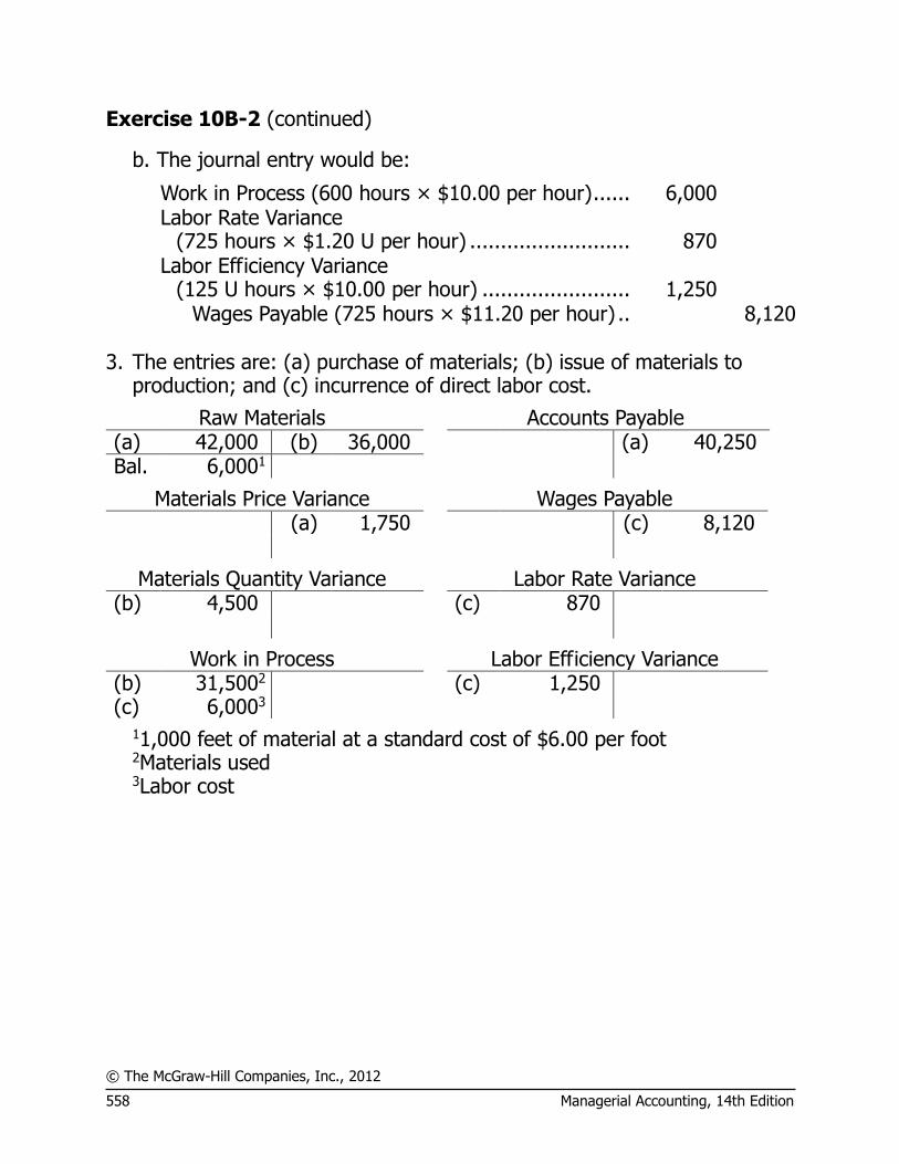
© The McGraw-Hill Companies, Inc., 2012
558 Managerial Accounting, 14th Edition
Exercise 10B-2 (continued)
b. The journal entry would be:
Work in Process (600 hours × $10.00 per hour) ...... 6,000 Labor Rate Variance
(725 hours × $1.20 U per hour) .......................... 870 Labor Efficiency Variance
(125 U hours × $10.00 per hour) ........................ 1,250 Wages Payable (725 hours × $11.20 per hour) .. 8,120
3. The entries are: (a) purchase of materials; (b) issue of materials to
production; and (c) incurrence of direct labor cost.
Raw Materials Accounts Payable (a) 42,000 (b) 36,000 (a) 40,250 Bal. 6,0001
Materials Price Variance Wages Payable (a) 1,750 (c) 8,120
Materials Quantity Variance Labor Rate Variance (b) 4,500 (c) 870
Work in Process Labor Efficiency Variance (b) 31,5002 (c) 1,250 (c) 6,0003
11,000 feet of material at a standard cost of $6.00 per foot 2Materials used 3Labor cost
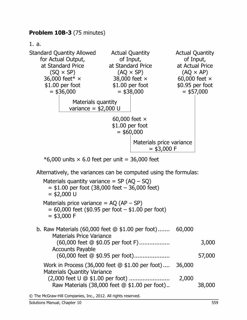
© The McGraw-Hill Companies, Inc., 2012. All rights reserved.
Solutions Manual, Chapter 10 559
Problem 10B-3 (75 minutes)
1. a.
Standard Quantity Allowed for Actual Output, at Standard Price
(SQ × SP)
Actual Quantity of Input,
at Standard Price (AQ × SP)
Actual Quantity of Input,
at Actual Price (AQ × AP)
36,000 feet* × $1.00 per foot
= $36,000
38,000 feet × $1.00 per foot
= $38,000
60,000 feet × $0.95 per foot
= $57,000
Materials quantity variance = $2,000 U
60,000 feet × $1.00 per foot
= $60,000
Materials price variance = $3,000 F
*6,000 units × 6.0 feet per unit = 36,000 feet Alternatively, the variances can be computed using the formulas:
Materials quantity variance = SP (AQ – SQ) = $1.00 per foot (38,000 feet – 36,000 feet) = $2,000 U
Materials price variance = AQ (AP – SP) = 60,000 feet ($0.95 per foot – $1.00 per foot) = $3,000 F
b. Raw Materials (60,000 feet @ $1.00 per foot) ....... 60,000
Materials Price Variance
(60,000 feet @ $0.05 per foot F) .................. 3,000
Accounts Payable
(60,000 feet @ $0.95 per foot) ..................... 57,000
Work in Process (36,000 feet @ $1.00 per foot) .... 36,000
Materials Quantity Variance
(2,000 feet U @ $1.00 per foot) ........................ 2,000 Raw Materials (38,000 feet @ $1.00 per foot) .. 38,000

© The McGraw-Hill Companies, Inc., 2012
560 Managerial Accounting, 14th Edition
Problem 10B-3 (continued)
2. a. Standard Hours Allowed
for Actual Output, at Standard Rate
(SH × SR)
Actual Hours of Input, at Standard Rate
(AH × SR)
Actual Hours of Input, at Actual Rate
(AH × AR) 6,000 hours** × $4.50 per hour
= $27,000
6,500 hours* × $4.50 per hour
= $29,250 $27,950
Labor efficiency variance = $2,250 U
Labor rate variance = $1,300 F
Spending variance = $950 U
* The actual hours worked during the period can be computed through the variable overhead efficiency variance, as follows:
SR (AH – SH) = Efficiency variance $3 per hour (AH – 6,000 hours**) = $1,500 U $3 per hour × AH – $18,000 = $1,500*** $3 per hour × AH = $19,500 AH = 6,500 hours
** 6,000 units × 1.0 hour per unit = 6,000 hours *** When used with the formula, unfavorable variances are positive
and favorable variances are negative. Alternatively, the variances can be computed using the formulas:
Labor efficiency variance = SR (AH – SH) = $4.50 per hour (6,500 hours – 6,000 hours) = $2,250 U
Labor rate variance = AH × (AR – SR) = 6,500 hours ($4.30 per hour* – $4.50 per hour) = $1,300 F
*$27,950 ÷ 6,500 hours = $4.30 per hour

© The McGraw-Hill Companies, Inc., 2012. All rights reserved.
Solutions Manual, Chapter 10 561
Problem 10B-3 (continued)
b. Work in Process (6,000 hours @ $4.50 per hour) .................... 27,000
Labor Efficiency Variance
(500 hours U @ $4.50 per hour) .................... 2,250
Labor Rate Variance
(6,500 hours @ $0.20 per hour F) ............ 1,300
Wages Payable
(6,500 hours @ $4.30 per hour) ............... 27,950 3. a. Standard Hours Allowed
for Actual Output, at Standard Rate
(SH × SR)
Actual Hours of Input, at Standard Rate
(AH × SR)
Actual Hours of Input, at Actual Rate
(AH × AR) 6,000 hours × $3.00 per hour
= $18,000
6,500 hours × $3.00 per hour
= $19,500 $20,475
Variable overhead efficiency variance
= $1,500 U
Variable overhead rate variance
= $975 U
Spending variance = $2,475 U Alternatively, the variances can be computed using the formulas:
Variable overhead efficiency variance = SR (AH – SH) = $3.00 per hour (6,500 hours – 6,000 hours) = $1,500 U
Variable overhead rate variance = AH × (AR – SR) = 6,500 hours ($3.15 per hour* – $3.00 per hour) = $975 U
*$20,475 ÷ 6,500 hours = $3.15 per hour
© The McGraw-Hill Companies, Inc., 2012
562 Managerial Accounting, 14th Edition
Problem 10B-3 (continued)
b. No. When variable manufacturing overhead is applied on the basis of direct labor-hours, it is impossible to have an unfavorable variable manufacturing overhead efficiency variance when the direct labor efficiency variance is favorable. The variable manufacturing overhead efficiency variance is the same as the direct labor efficiency variance except that the difference between actual hours and the standard hours allowed for the output is multiplied by a different rate. If the direct labor efficiency variance is favorable, the variable manufacturing overhead efficiency variance must also be favorable.
4. For materials:
Favorable price variance: Decrease in outside purchase prices, fortunate buy, inferior quality materials, unusual discounts due to quantity purchased, inaccurate standards.
Unfavorable quantity variance: Inferior quality materials, carelessness, poorly adjusted machines, unskilled workers, inaccurate standards.
For labor:
Favorable rate variance: Unskilled workers (paid lower rates), piecework, inaccurate standards.
Unfavorable efficiency variance: Poorly trained workers, poor quality materials, faulty equipment, work interruptions, fixed labor with insufficient demand to keep them all busy, inaccurate standards.
For variable overhead:
Unfavorable rate variance: Increase in supplier prices, inaccurate standards, waste, theft of supplies.
Unfavorable efficiency variance: See comments under direct labor efficiency variance.
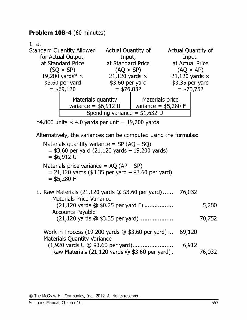
© The McGraw-Hill Companies, Inc., 2012. All rights reserved.
Solutions Manual, Chapter 10 563
Problem 10B-4 (60 minutes)
1. a. Standard Quantity Allowed
for Actual Output, at Standard Price
(SQ × SP)
Actual Quantity of Input,
at Standard Price (AQ × SP)
Actual Quantity of Input,
at Actual Price (AQ × AP)
19,200 yards* × $3.60 per yard
= $69,120
21,120 yards × $3.60 per yard
= $76,032
21,120 yards × $3.35 per yard
= $70,752
Materials quantity variance = $6,912 U
Materials price variance = $5,280 F
Spending variance = $1,632 U
*4,800 units × 4.0 yards per unit = 19,200 yards Alternatively, the variances can be computed using the formulas:
Materials quantity variance = SP (AQ – SQ) = $3.60 per yard (21,120 yards – 19,200 yards) = $6,912 U
Materials price variance = AQ (AP – SP) = 21,120 yards ($3.35 per yard – $3.60 per yard) = $5,280 F
b. Raw Materials (21,120 yards @ $3.60 per yard) ...... 76,032
Materials Price Variance
(21,120 yards @ $0.25 per yard F) ................. 5,280
Accounts Payable
(21,120 yards @ $3.35 per yard) .................... 70,752 Work in Process (19,200 yards @ $3.60 per yard) ... 69,120
Materials Quantity Variance
(1,920 yards U @ $3.60 per yard) ........................ 6,912 Raw Materials (21,120 yards @ $3.60 per yard) . 76,032
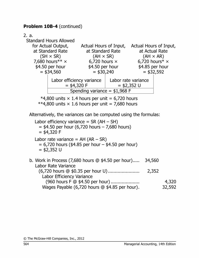
© The McGraw-Hill Companies, Inc., 2012
564 Managerial Accounting, 14th Edition
Problem 10B-4 (continued)
2. a. Standard Hours Allowed
for Actual Output, at Standard Rate
(SH × SR)
Actual Hours of Input, at Standard Rate
(AH × SR)
Actual Hours of Input, at Actual Rate
(AH × AR) 7,680 hours** × $4.50 per hour
= $34,560
6,720 hours × $4.50 per hour
= $30,240
6,720 hours* × $4.85 per hour
= $32,592
Labor efficiency variance = $4,320 F
Labor rate variance = $2,352 U
Spending variance = $1,968 F
* 4,800 units × 1.4 hours per unit = 6,720 hours ** 4,800 units × 1.6 hours per unit = 7,680 hours
Alternatively, the variances can be computed using the formulas:
Labor efficiency variance = SR (AH – SH) = $4.50 per hour (6,720 hours – 7,680 hours) = $4,320 F
Labor rate variance = AH (AR – SR) = 6,720 hours ($4.85 per hour – $4.50 per hour) = $2,352 U
b. Work in Process (7,680 hours @ $4.50 per hour) ..... 34,560
Labor Rate Variance
(6,720 hours @ $0.35 per hour U) ....................... 2,352
Labor Efficiency Variance
(960 hours F @ $4.50 per hour) ..................... 4,320 Wages Payable (6,720 hours @ $4.85 per hour) . 32,592

© The McGraw-Hill Companies, Inc., 2012. All rights reserved.
Solutions Manual, Chapter 10 565
Problem 10B-4 (continued)
3. Standard Hours Allowed
for Actual Output, at Standard Rate
(SH × SR)
Actual Hours of Input, at Standard Rate
(AH × SR)
Actual Hours of Input, at Actual Rate
(AH × AR) 7,680 hours × $1.80 per hour
= $13,824
6,720 hours × $1.80 per hour
= $12,096
6,720 hours × $2.15 per hour
= $14,448
Variable overhead efficiency variance
= $1,728 F
Variable overhead rate variance = $2,352 U
Spending variance = $624 U Alternatively, the variances can be computed using the formulas:
Variable overhead efficiency variance = SR (AH – SH) = $1.80 per hour (6,720 hours – 7,680 hours) = $1,728 F
Variable overhead rate variance = AH (AR – SR) = 6,720 hours ($2.15 per hour – $1.80 per hour) = $2,352 U 4. No. This total variance is made up of several quite large individual
variances, some of which may warrant investigation. A summary of variances is given below:
Materials: Quantity variance ............................. $6,912 U Price variance .................................. 5,280 F $1,632 U
Labor: Efficiency variance ........................... 4,320 F Rate variance................................... 2,352 U 1,968 F
Variable overhead: Efficiency variance ........................... 1,728 F Spending variance ............................ 2,352 U 624 U
Net unfavorable variance .................... $ 288 U
© The McGraw-Hill Companies, Inc., 2012
566 Managerial Accounting, 14th Edition
Problem 10B-4 (continued)
5. The variances have many possible causes. Some of the more likely causes include:
Materials variances:
Favorable price variance: Good price, inaccurate standards, inferior quality materials, unusual discount due to quantity purchased, drop in market price.
Unfavorable quantity variance: Carelessness, poorly adjusted machines, unskilled workers, inferior quality materials, inaccurate standards.
Labor variances:
Unfavorable rate variance: Use of highly skilled workers, change in wage rates, inaccurate standards, overtime.
Favorable efficiency variance: Use of highly skilled workers, high-quality materials, new equipment, inaccurate standards.
Variable overhead variances:
Unfavorable rate variance: Increase in costs, inaccurate standards, waste, theft, spillage, purchases in uneconomical lots.
Favorable efficiency variance: Same as for labor efficiency variance.
© The McGraw-Hill Companies, Inc., 2012. All rights reserved.
Solutions Manual, Chapter 10 567
Case 10B-5 (30 minutes)
This case may be difficult for some students to grasp because it requires looking at standard costs from an entirely different perspective. In this case, standard costs have been inappropriately used as a means to manipulate reported earnings rather than as a way to control costs. 1. Lansing has evidently set very loose standards in which the standard
prices and standard quantities are far too high. This guarantees that favorable variances will ordinarily result from operations. If the standard costs are set artificially high, the standard cost of goods sold will be artificially high and thus the division’s net operating income will be depressed until the favorable variances are recognized. If Lansing saves the favorable variances, he can release just enough in the second and third quarters to show some improvement and then he can release all of the rest in the last quarter, creating the annual “Christmas present.”
2. Lansing should not be permitted to continue this practice for several
reasons. First, it distorts the quarterly earnings for both the division and the company. The distortions of the division’s quarterly earnings are troubling because the manipulations may mask real signs of trouble. The distortions of the company’s quarterly earnings are troubling because they may mislead external users of the financial statements. Second, Lansing should not be rewarded for manipulating earnings. This sets a moral tone in the company that is likely to lead to even deeper trouble. Indeed, the permissive attitude of top management toward the manipulation of earnings may indicate the existence of other, even more serious, ethical problems in the company. Third, a clear message should be sent to division managers like Lansing that their job is to manage their operations, not their earnings. If they keep on top of operations and manage well, the earnings should take care of themselves.
© The McGraw-Hill Companies, Inc., 2012
568 Managerial Accounting, 14th Edition
Case 10B-5 (continued)
3. Stacy Cummins does not have any easy alternatives available. She has already taken the problem to the President, who was not interested. If she goes around the President to the Board of Directors, she will be putting herself in a politically difficult position with little likelihood that it will do much good if, in fact, the Board of Directors already knows what is going on.
On the other hand, if she simply goes along, she will be violating the Credibility standard of ethical conduct for management accountants. The Home Security Division’s manipulation of quarterly earnings does distort the entire company’s quarterly reports. And the Credibility standard clearly stipulates that management accountants have a responsibility to “disclose all relevant information that could reasonably be expected to influence an intended user’s understanding of the reports, analyses, or recommendations.” Apart from the ethical issue, there is also a very practical consideration. If Merced Home Products becomes embroiled in controversy concerning questionable accounting practices, Stacy Cummins will be viewed as a responsible party by outsiders and her career is likely to suffer dramatically and she may even face legal problems.
We would suggest that Ms. Cummins quietly bring the manipulation of earnings to the attention of the audit committee of the Board of Directors, carefully laying out in a non-confrontational manner the problems created by Lansing’s practice of manipulating earnings. If the President and the Board of Directors are still not interested in dealing with the problem, she may reasonably conclude that the best alternative is to start looking for another job.

© The McGraw-Hill Companies, Inc., 2012
Solutions Manual, Chapter 13 703
Chapter 13 Capital Budgeting Decisions
Solutions to Questions
13-1 A capital budgeting screening decision is concerned with whether a proposed investment project passes a preset hurdle, such as a 15% rate of return. A capital budgeting preference decision is concerned with choosing from among two or more alternative investment projects, each of which has passed the hurdle.
13-2 The “time value of money” refers to the fact that a dollar received today is more valuable than a dollar received in the future simply because a dollar received today can be invested to yield more than a dollar in the future.
13-3 Discounting is the process of computing the present value of a future cash flow. Discounting gives recognition to the time value of money and makes it possible to meaningfully add together cash flows that occur at different times.
13-4 Accounting net income is based on accruals rather than on cash flows. Both the net present value and internal rate of return methods focus on cash flows.
13-5 Unlike other common capital budgeting methods, discounted cash flow methods recognize the time value of money and take into account all future cash flows.
13-6 Net present value is the present value of cash inflows less the present value of the cash outflows. The net present value can be negative if the present value of the outflows is greater than the present value of the inflows.
13-7 One assumption is that all cash flows occur at the end of a period. Another is that all cash inflows are immediately reinvested at a rate of return equal to the discount rate.
13-8 No. The cost of capital is not simply the interest paid on long-term debt. The cost of capital is a weighted average of the costs of all sources of financing, both debt and equity.
13-9 The internal rate of return is the rate of return on an investment project over its life. It is computed by finding the discount rate that results in a zero net present value for the project.
13-10 The cost of capital is a hurdle that must be cleared before an investment project will be accepted. In the case of the net present value method, the cost of capital is used as the discount rate. If the net present value of the project is positive, then the project is acceptable because its rate of return is greater than the cost of capital. In the case of the internal rate of return method, the cost of capital is compared to a project’s internal rate of return. If the project’s internal rate of return is greater than the cost of capital, then the project is acceptable.
13-11 No. As the discount rate increases, the present value of a given future cash flow decreases. For example, the present value factor for a discount rate of 12% for cash to be received ten years from now is 0.322, whereas the present value factor for a discount rate of 14% over the same period is 0.270. If the cash to be received in ten years is $10,000, the present value in the first case is $3,220, but only $2,700 in the second case. Thus, as the discount rate increases, the present value of a given future cash flow decreases.
13-12 The internal rate of return is more than 14% because the net present value is positive. The internal rate of return would be 14% only if the net present value (evaluated using a 14%

© The McGraw-Hill Companies, Inc., 2012
704 Managerial Accounting, 14th Edition
discount rate) is zero. The internal rate of return would be less than 14% if the net present value (evaluated using a 14% discount rate) is negative.
13-13 The project profitability index is computed by dividing the net present value of the cash flows from an investment project by the required investment. The index measures the profit (in terms of net present value) provided by each dollar of investment in a project. The higher the project profitability index, the more desirable is the investment project.
13-14 The payback period is the length of time for an investment to fully recover its initial cost
out of the cash receipts that it generates. The payback method is used as a screening tool for investment proposals. The payback method is useful when a company has cash flow problems. The payback method is also used in industries where obsolescence is very rapid.
13-15 Neither the payback method nor the simple rate of return method considers the time value of money. Under both methods, a dollar received in the future is weighed the same as a dollar received today. Furthermore, the payback method ignores all cash flows that occur after the initial investment has been recovered.

© The McGraw-Hill Companies, Inc., 2012
Solutions Manual, Chapter 13 705
Exercise 13-1 (10 minutes)
1.
Item Year(s) Cash Flow 12%
Factor
Present Value of
Cash Flows
Annual cost savings .. 1-10 $4,000 5.650 $ 22,600 Initial investment ..... Now $(25,000) 1.000 (25,000) Net present value ..... $ (2,400)
2.
Item Cash Flow Years
Total Cash Flows
Annual cost savings .. $4,000 10 $ 40,000 Initial investment ..... $(25,000) 1 (25,000) Net cash flow ........... $ 15,000

© The McGraw-Hill Companies, Inc., 2012
706 Managerial Accounting, 14th Edition
Exercise 13-2 (30 minutes)
1. Annual savings over present method of delivery ........ $5,400
Added contribution margin from expanded deliveries
(1,800 pizzas × $2 per pizza) ................................ 3,600 Annual cash inflows ................................................. $9,000
2. Investment requiredFactor of the internal =
rate of return Annual cash inflow
$45,000= = 5.000
$9,000
Looking in Exhibit 13B-2, and scanning along the six-year line, we can
see that the factor computed above, 5.000, is closest to 5.076, the factor for the 5% rate of return. Therefore, to the nearest whole percent, the internal rate of return is 5%.
3. The cash flows are not even over the six-year life of the truck because
of the extra $13,000 cash inflow that occurs in the sixth year. Therefore, the approach used above cannot be used to compute the internal rate of return. Using trial-and-error or some other method, the internal rate of return turns out to be about 11%:
Year(s) Amount of Cash Flows
11% Factor
Present Value of Cash Flows
Initial investment ..... Now $(45,000) 1.000 $(45,000) Annual cash inflows .. 1-6 $9,000 4.231 38,079 Salvage value ........... 6 $13,000 0.535 6,955 Net present value ..... $ 34
As expected, the extra cash inflow in the sixth year increases the internal rate of return.
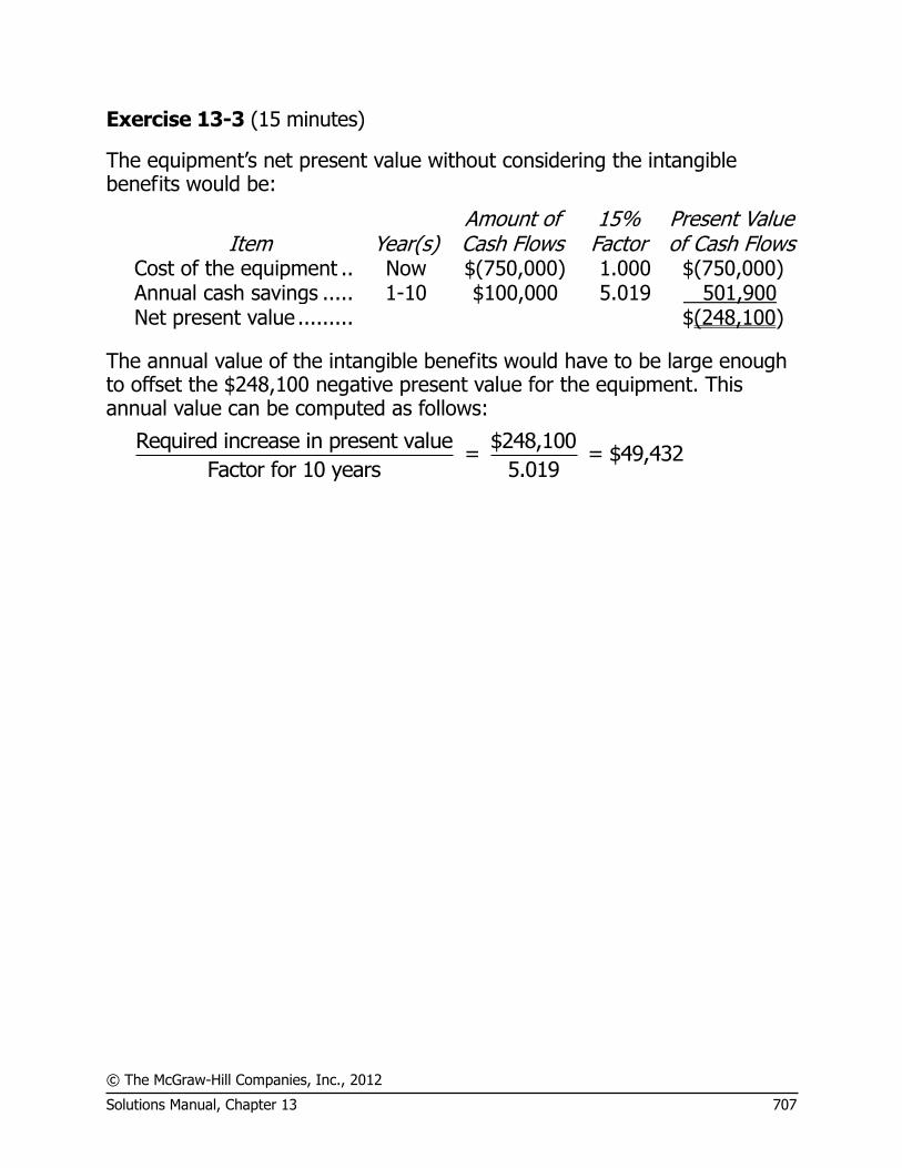
© The McGraw-Hill Companies, Inc., 2012
Solutions Manual, Chapter 13 707
Exercise 13-3 (15 minutes)
The equipment’s net present value without considering the intangible benefits would be:
Item Year(s) Amount of Cash Flows
15% Factor
Present Value of Cash Flows
Cost of the equipment .. Now $(750,000) 1.000 $(750,000) Annual cash savings ..... 1-10 $100,000 5.019 501,900 Net present value ......... $(248,100)
The annual value of the intangible benefits would have to be large enough to offset the $248,100 negative present value for the equipment. This annual value can be computed as follows:
Required increase in present value $248,100 = = $49,432
Factor for 10 years 5.019

© The McGraw-Hill Companies, Inc., 2012
708 Managerial Accounting, 14th Edition
Exercise 13-4 (10 minutes)
1. The project profitability index for each proposal is:
Proposal
Net Present Value (a)
Investment Required
(b)
Project Profitability
Index (a) ÷ (b)
A $34,000 $85,000 0.40 B $50,000 $200,000 0.25 C $45,000 $90,000 0.50 D $51,000 $170,000 0.30
2. The ranking is:
Proposal
Project Profitability
Index C 0.50 A 0.40 D 0.30 B 0.25
Note that proposals D and B have the highest net present values of the four proposals, but they rank at the bottom of the list in terms of the project profitability index.
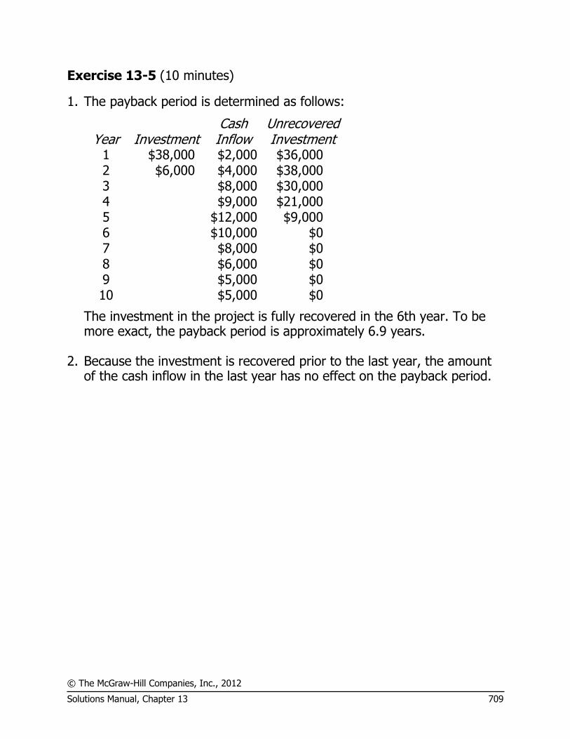
© The McGraw-Hill Companies, Inc., 2012
Solutions Manual, Chapter 13 709
Exercise 13-5 (10 minutes)
1. The payback period is determined as follows:
Year Investment Cash
Inflow Unrecovered Investment
1 $38,000 $2,000 $36,000 2 $6,000 $4,000 $38,000 3 $8,000 $30,000 4 $9,000 $21,000 5 $12,000 $9,000 6 $10,000 $0 7 $8,000 $0 8 $6,000 $0 9 $5,000 $0 10 $5,000 $0
The investment in the project is fully recovered in the 6th year. To be more exact, the payback period is approximately 6.9 years.
2. Because the investment is recovered prior to the last year, the amount
of the cash inflow in the last year has no effect on the payback period.

© The McGraw-Hill Companies, Inc., 2012
710 Managerial Accounting, 14th Edition
Exercise 13-6 (10 minutes)
The annual incremental net operating income is determined by comparing the operating cost of the old machine to the operating cost of the new machine and the depreciation that would be taken on the new machine:
Operating cost of old machine ...................... $33,000 Less operating cost of new machine ............. 10,000 Less annual depreciation on the new machine
($80,000 ÷ 10 years) ................................ 8,000 Annual incremental net operating income ..... $15,000
Cost of the new machine ............................. $80,000 Less scrap value of old machine ................... 5,000 Initial investment ......................................... $75,000
Annual incremental net operating incomeSimple rate = of return Initial investment
$15,000= = 20%
$75,000
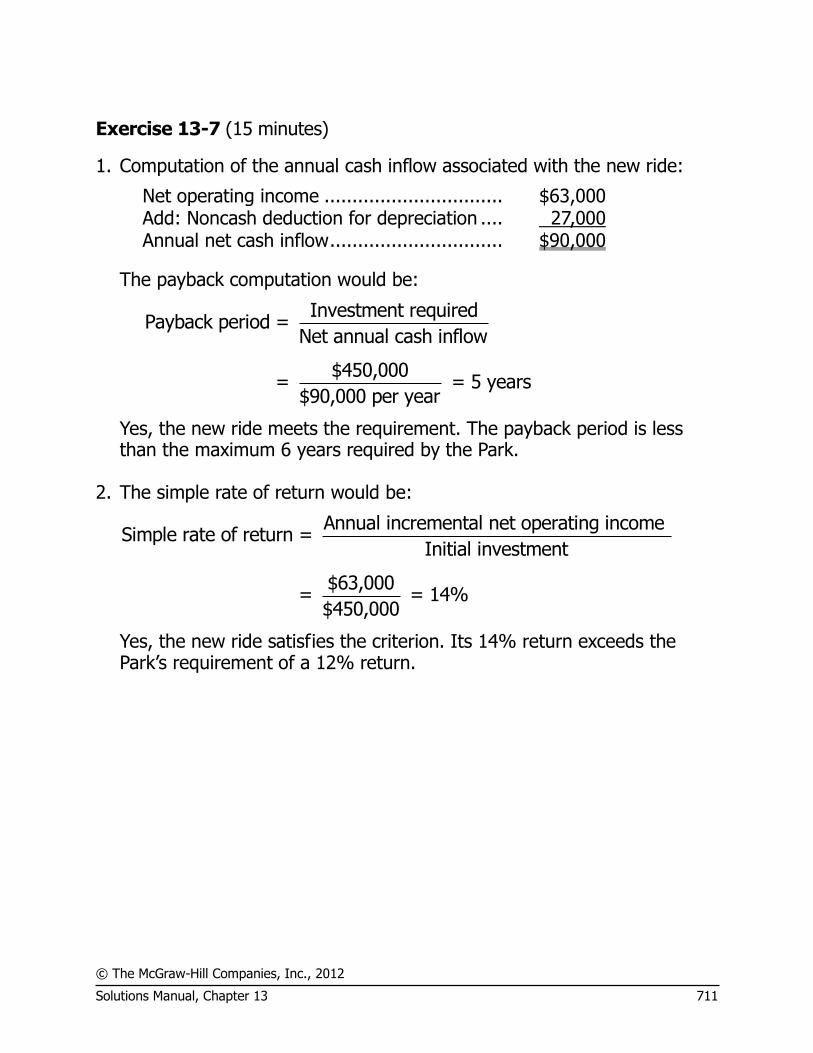
© The McGraw-Hill Companies, Inc., 2012
Solutions Manual, Chapter 13 711
Exercise 13-7 (15 minutes)
1. Computation of the annual cash inflow associated with the new ride:
Net operating income ................................ $63,000 Add: Noncash deduction for depreciation .... 27,000 Annual net cash inflow ............................... $90,000
The payback computation would be:
Investment requiredPayback period =
Net annual cash inflow
$450,000= = 5 years
$90,000 per year
Yes, the new ride meets the requirement. The payback period is less than the maximum 6 years required by the Park.
2. The simple rate of return would be:
Annual incremental net operating income Simple rate of return =
Initial investment
$63,000= = 14%
$450,000
Yes, the new ride satisfies the criterion. Its 14% return exceeds the Park’s requirement of a 12% return.

© The McGraw-Hill Companies, Inc., 2012
712 Managerial Accounting, 14th Edition
Exercise 13-8 (10 minutes)
1. Note: All present value factors have been taken from Exhibit 13B-1 in Appendix 13B, using a 16% discount rate.
Investment in the equipment .................. $134,650 Less present value of Year 1 and
Year 2 cash inflows: Year 1: $45,000 × 0.862 ................... $38,790 Year 2: $60,000 × 0.743 .................... 44,580 83,370
Present value of Year 3 cash inflow ......... $ 51,280
Therefore, the expected cash inflow for Year 3 is:
$51,280 ÷ 0.641 = $80,000.
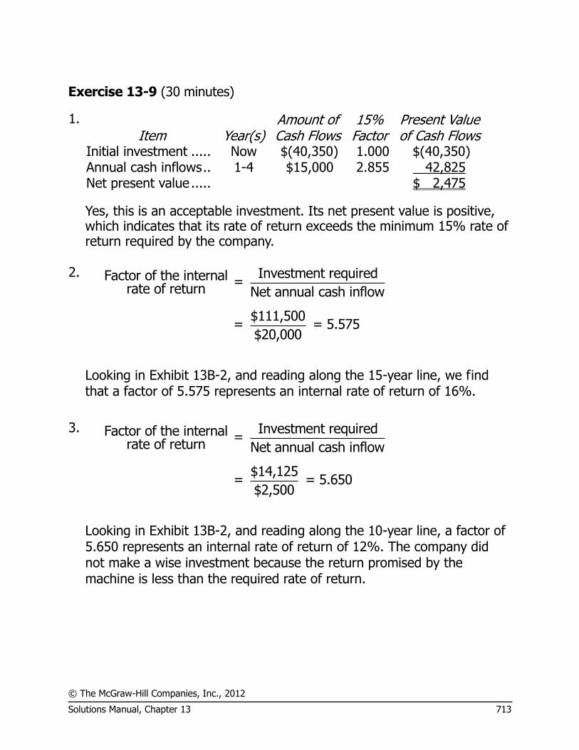
© The McGraw-Hill Companies, Inc., 2012
Solutions Manual, Chapter 13 713
Exercise 13-9 (30 minutes)
1.
Item Year(s) Amount of Cash Flows
15% Factor
Present Value of Cash Flows
Initial investment ..... Now $(40,350) 1.000 $(40,350) Annual cash inflows .. 1-4 $15,000 2.855 42,825 Net present value ..... $ 2,475
Yes, this is an acceptable investment. Its net present value is positive, which indicates that its rate of return exceeds the minimum 15% rate of return required by the company.
2. Investment requiredFactor of the internal =
rate of return Net annual cash inflow
$111,500= = 5.575
$20,000
Looking in Exhibit 13B-2, and reading along the 15-year line, we find that a factor of 5.575 represents an internal rate of return of 16%.
3. Investment requiredFactor of the internal =
rate of return Net annual cash inflow
$14,125= = 5.650
$2,500
Looking in Exhibit 13B-2, and reading along the 10-year line, a factor of 5.650 represents an internal rate of return of 12%. The company did not make a wise investment because the return promised by the machine is less than the required rate of return.
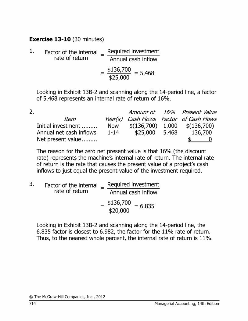
© The McGraw-Hill Companies, Inc., 2012
714 Managerial Accounting, 14th Edition
Exercise 13-10 (30 minutes)
1. Required investmentFactor of the internal = rate of return Annual cash inflow
$136,700= = 5.468
$25,000
Looking in Exhibit 13B-2 and scanning along the 14-period line, a factor
of 5.468 represents an internal rate of return of 16%. 2.
Item Year(s) Amount of Cash Flows
16% Factor
Present Value of Cash Flows
Initial investment ......... Now $(136,700) 1.000 $(136,700) Annual net cash inflows 1-14 $25,000 5.468 136,700 Net present value ......... $ 0
The reason for the zero net present value is that 16% (the discount rate) represents the machine’s internal rate of return. The internal rate of return is the rate that causes the present value of a project’s cash inflows to just equal the present value of the investment required.
3. Required investmentFactor of the internal =
rate of return Annual cash inflow
$136,700= = 6.835
$20,000
Looking in Exhibit 13B-2 and scanning along the 14-period line, the
6.835 factor is closest to 6.982, the factor for the 11% rate of return. Thus, to the nearest whole percent, the internal rate of return is 11%.

© The McGraw-Hill Companies, Inc., 2012
Solutions Manual, Chapter 13 715
Exercise 13-11 (10 minutes)
Item Year(s) Amount of Cash Flows
16% Factor
Present Value of
Cash Flows Project A:
Investment required . Now $(15,000) 1.000 $(15,000) Annual cash inflows .. 1-10 $4,000 4.833 19,332 Net present value ..... $ 4,332
Project B:
Investment .............. Now $(15,000) 1.000 $(15,000) Cash inflow .............. 10 $60,000 0.227 13,620 Net present value ..... $ (1,380)
Project A should be selected. Project B does not provide the required 16% return, as shown by its negative net present value.
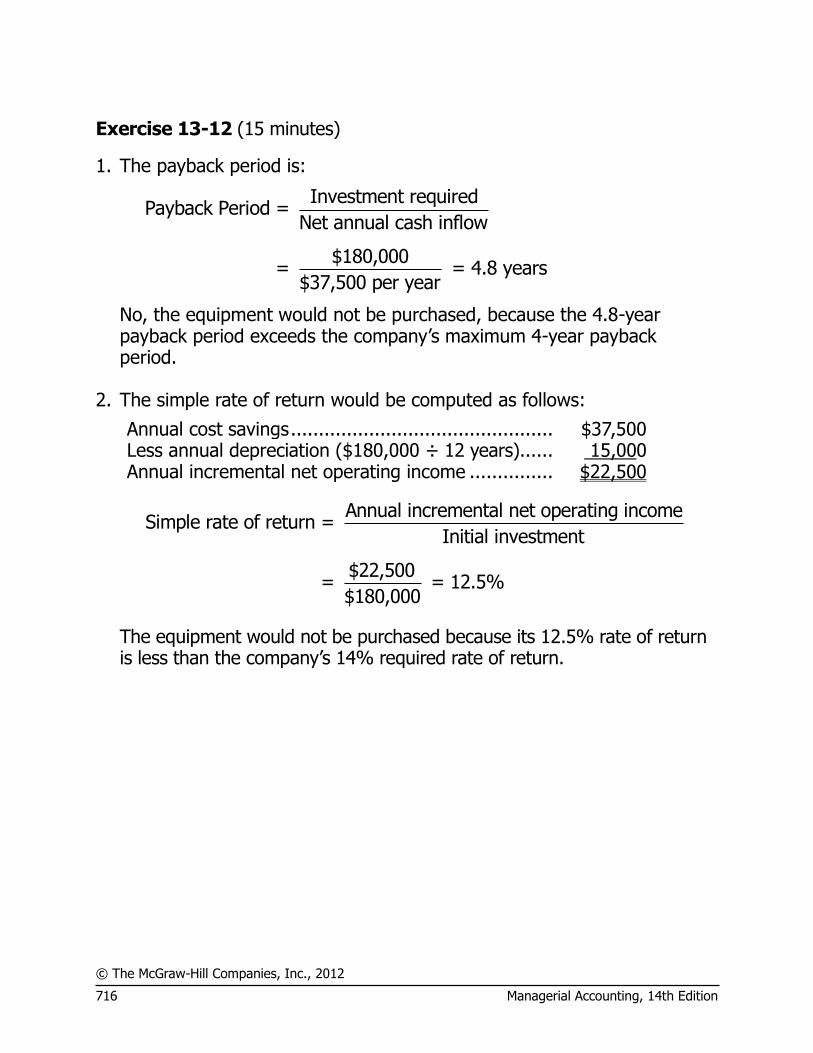
© The McGraw-Hill Companies, Inc., 2012
716 Managerial Accounting, 14th Edition
Exercise 13-12 (15 minutes)
1. The payback period is:
Investment requiredPayback Period =
Net annual cash inflow
$180,000= = 4.8 years
$37,500 per year
No, the equipment would not be purchased, because the 4.8-year payback period exceeds the company’s maximum 4-year payback period.
2. The simple rate of return would be computed as follows:
Annual cost savings ............................................... $37,500 Less annual depreciation ($180,000 ÷ 12 years)...... 15,000 Annual incremental net operating income ............... $22,500
Annual incremental net operating incomeSimple rate of return =
Initial investment
$22,500= = 12.5%
$180,000
The equipment would not be purchased because its 12.5% rate of return is less than the company’s 14% required rate of return.
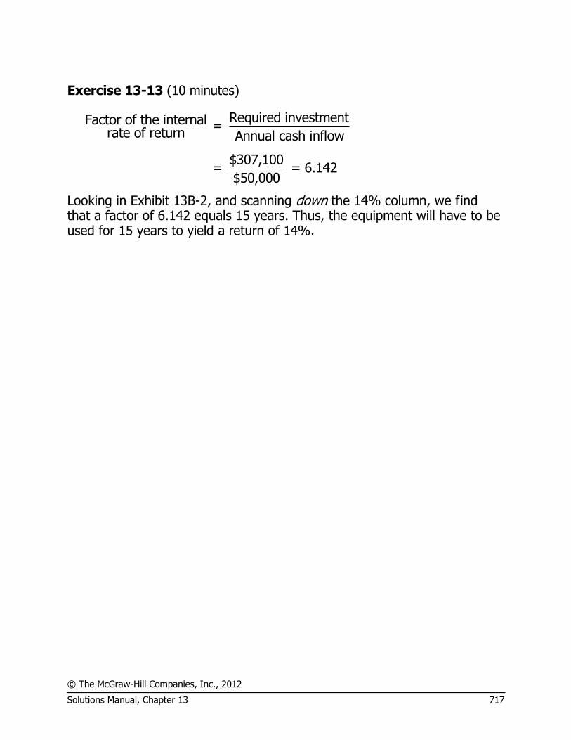
© The McGraw-Hill Companies, Inc., 2012
Solutions Manual, Chapter 13 717
Exercise 13-13 (10 minutes)
Required investmentFactor of the internal = rate of return Annual cash inflow
$307,100= = 6.142
$50,000
Looking in Exhibit 13B-2, and scanning down the 14% column, we find that a factor of 6.142 equals 15 years. Thus, the equipment will have to be used for 15 years to yield a return of 14%.

© The McGraw-Hill Companies, Inc., 2012
718 Managerial Accounting, 14th Edition
Exercise 13-14 (15 minutes)
Item Year(s)
Amount of Cash Flows
20% Factor
Present Value of
Cash Flows
Project A: Cost of the equipment ............... Now $(300,000) 1.000 $(300,000) Annual cash inflows ................... 1-7 $80,000 3.605 288,400 Salvage value of the equipment . 7 $20,000 0.279 5,580 Net present value ...................... $ (6,020)
Project B:
Working capital investment ........ Now $(300,000) 1.000 $(300,000) Annual cash inflows ................... 1-7 $60,000 3.605 216,300 Working capital released ............ 7 $300,000 0.279 83,700 Net present value ...................... $ 0
The $300,000 should be invested in Project B rather than in Project A. Project B has a zero net present value, which means that it promises exactly a 20% rate of return. Project A is not acceptable at all, since it has a negative net present value.
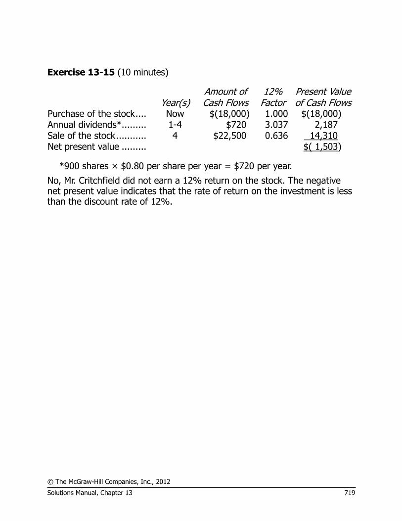
© The McGraw-Hill Companies, Inc., 2012
Solutions Manual, Chapter 13 719
Exercise 13-15 (10 minutes)
Year(s) Amount of Cash Flows
12% Factor
Present Value of Cash Flows
Purchase of the stock .... Now $(18,000) 1.000 $(18,000) Annual dividends*......... 1-4 $720 3.037 2,187 Sale of the stock ........... 4 $22,500 0.636 14,310 Net present value ......... $( 1,503)
*900 shares × $0.80 per share per year = $720 per year.
No, Mr. Critchfield did not earn a 12% return on the stock. The negative net present value indicates that the rate of return on the investment is less than the discount rate of 12%.

© The McGraw-Hill Companies, Inc., 2012
720 Managerial Accounting, 14th Edition
Problem 13-16 (15 minutes)
Item Year(s)
Amount of Cash Flows
14% Factor
Present Value of
Cash Flows
Cost of equipment required ...... Now $(850,000) 1.000 $(850,000) Working capital required .......... Now $(100,000) 1.000 (100,000) Annual net cash receipts .......... 1-5 $230,000 3.433 789,590 Cost of road repairs ................. 3 $(60,000) 0.675 (40,500) Salvage value of equipment ...... 5 $200,000 0.519 103,800 Working capital released .......... 5 $100,000 0.519 51,900 Net present value .................... $ (45,210)
No, the project should not be accepted; it has a negative net present value. This means that the rate of return on the investment is less than the company’s required rate of return of 14%.

© The McGraw-Hill Companies, Inc., 2012
Solutions Manual, Chapter 13 721
Problem 13-17 (30 minutes)
1. The formula for the project profitability index is:
Net present value
Project profitability index = Investment required
The index for the projects under consideration would be:
Project 1: $87,270 ÷ $480,000 = 0.182 Project 2: $73,400 ÷ $360,000 = 0.204 Project 3: $66,140 ÷ $270,000 = 0.245 Project 4: $72,970 ÷ $450,000 = 0.162 2. a., b., and c.
Net Present
Value
Project Profitability
Index Internal Rate
of Return First preference ........ 1 3 4 Second preference .... 2 2 3 Third preference ....... 4 1 1 Fourth preference ..... 3 4 2
3. Which ranking is best will depend on the company’s opportunities for
reinvesting funds as they are released from a project. The internal rate of return method assumes that any released funds are reinvested at the internal rate of return. This means that funds released from project #4 would have to be reinvested at a rate of return of 19%, but another project yielding such a high rate of return might be difficult to find.
The project profitability index approach assumes that funds released from a project are reinvested at a rate of return equal to the discount rate, which in this case is only 10%. On balance, the project profitability index is generally regarded as the most dependable method of ranking competing projects.
The net present value is inferior to the project profitability index as a ranking device because it does not properly consider the amount of investment. For example, it ranks project #3 as fourth because of its low net present value; yet this project is the best in terms of the amount of cash inflow generated for each dollar of investment (as shown by the

© The McGraw-Hill Companies, Inc., 2012
722 Managerial Accounting, 14th Edition
project profitability index).
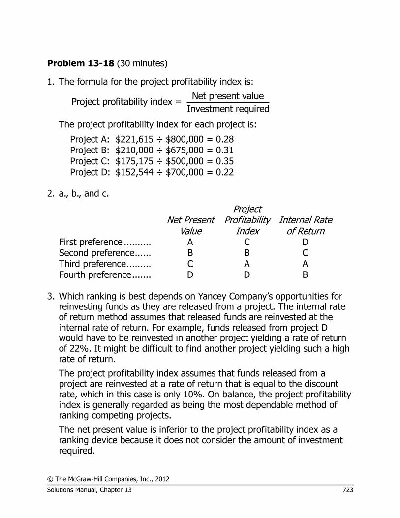
© The McGraw-Hill Companies, Inc., 2012
Solutions Manual, Chapter 13 723
Problem 13-18 (30 minutes)
1. The formula for the project profitability index is:
Net present value
Project profitability index = Investment required
The project profitability index for each project is:
Project A: $221,615 ÷ $800,000 = 0.28 Project B: $210,000 ÷ $675,000 = 0.31 Project C: $175,175 ÷ $500,000 = 0.35 Project D: $152,544 ÷ $700,000 = 0.22
2. a., b., and c.
Net Present
Value
Project Profitability
Index Internal Rate
of Return First preference .......... A C D Second preference ...... B B C Third preference ......... C A A Fourth preference ....... D D B
3. Which ranking is best depends on Yancey Company’s opportunities for
reinvesting funds as they are released from a project. The internal rate of return method assumes that released funds are reinvested at the internal rate of return. For example, funds released from project D would have to be reinvested in another project yielding a rate of return of 22%. It might be difficult to find another project yielding such a high rate of return.
The project profitability index assumes that funds released from a project are reinvested at a rate of return that is equal to the discount rate, which in this case is only 10%. On balance, the project profitability index is generally regarded as being the most dependable method of ranking competing projects.
The net present value is inferior to the project profitability index as a ranking device because it does not consider the amount of investment required.
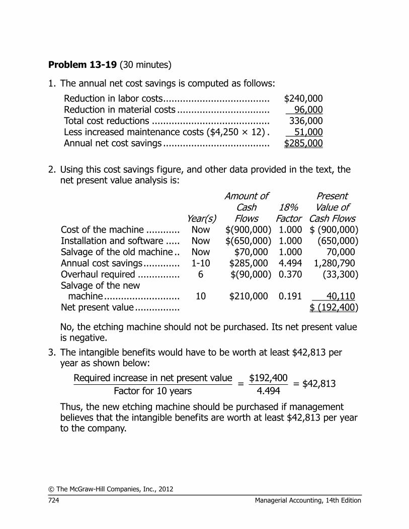
© The McGraw-Hill Companies, Inc., 2012
724 Managerial Accounting, 14th Edition
Problem 13-19 (30 minutes)
1. The annual net cost savings is computed as follows:
Reduction in labor costs ...................................... $240,000 Reduction in material costs ................................. 96,000 Total cost reductions .......................................... 336,000 Less increased maintenance costs ($4,250 × 12) . 51,000 Annual net cost savings ...................................... $285,000
2. Using this cost savings figure, and other data provided in the text, the
net present value analysis is:
Year(s)
Amount of Cash Flows
18% Factor
Present Value of
Cash Flows Cost of the machine ............ Now $(900,000) 1.000 $ (900,000) Installation and software ..... Now $(650,000) 1.000 (650,000) Salvage of the old machine .. Now $70,000 1.000 70,000 Annual cost savings ............. 1-10 $285,000 4.494 1,280,790 Overhaul required ............... 6 $(90,000) 0.370 (33,300)
Salvage of the new
machine ........................... 10 $210,000 0.191 40,110 Net present value ................ $ (192,400)
No, the etching machine should not be purchased. Its net present value is negative.
3. The intangible benefits would have to be worth at least $42,813 per year as shown below:
Required increase in net present value $192,400
= = $42,813Factor for 10 years 4.494
Thus, the new etching machine should be purchased if management believes that the intangible benefits are worth at least $42,813 per year to the company.
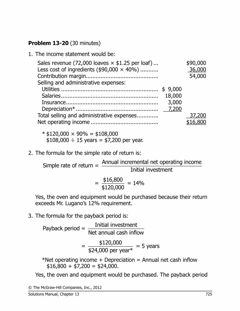
© The McGraw-Hill Companies, Inc., 2012
Solutions Manual, Chapter 13 725
Problem 13-20 (30 minutes)
1. The income statement would be:
Sales revenue (72,000 loaves × $1.25 per loaf) ... $90,000 Less cost of ingredients ($90,000 × 40%) ........... 36,000 Contribution margin............................................ 54,000 Selling and administrative expenses:
Utilities ........................................................... $ 9,000 Salaries ........................................................... 18,000 Insurance ........................................................ 3,000 Depreciation* .................................................. 7,200
Total selling and administrative expenses ............. 37,200 Net operating income ......................................... $16,800
* $120,000 × 90% = $108,000 $108,000 ÷ 15 years = $7,200 per year.
2. The formula for the simple rate of return is:
Annual incremental net operating incomeSimple rate of return =
Initial investment
$16,800= = 14%
$120,000
Yes, the oven and equipment would be purchased because their return exceeds Mr. Lugano’s 12% requirement.
3. The formula for the payback period is:
Initial investmentPayback period =
Net annual cash inflow
$120,000= = 5 years
$24,000 per year*
*Net operating income + Depreciation = Annual net cash inflow $16,800 + $7,200 = $24,000.
Yes, the oven and equipment would be purchased. The payback period
© The McGraw-Hill Companies, Inc., 2012
726 Managerial Accounting, 14th Edition
is less than the 6-year period Mr. Lugano requires.

© The McGraw-Hill Companies, Inc., 2012
Solutions Manual, Chapter 13 727
Problem 13-21 (20 minutes)
1. The annual net cash inflows would be:
Reduction in annual operating costs: Operating costs, present hand method ..... $35,000 Operating costs, new machine ................. 14,000 Annual savings in operating costs ............ 21,000
Increased annual contribution margin: 5,000 packages × $0.60 per package ....... 3,000
Total annual net cash inflows ..................... $24,000
2.
Item Year(s)
Amount of Cash Flows
16% Factor
Present Value of
Cash Flows
Cost of the machine ... Now $(90,000) 1.000 $(90,000) Overhaul required ...... 5 $(7,500) 0.476 (3,570)
Annual net cash
inflows .................... 1-8 $24,000 4.344 104,256 Salvage value ............. 8 $6,000 0.305 1,830 Net present value ....... $ 12,516
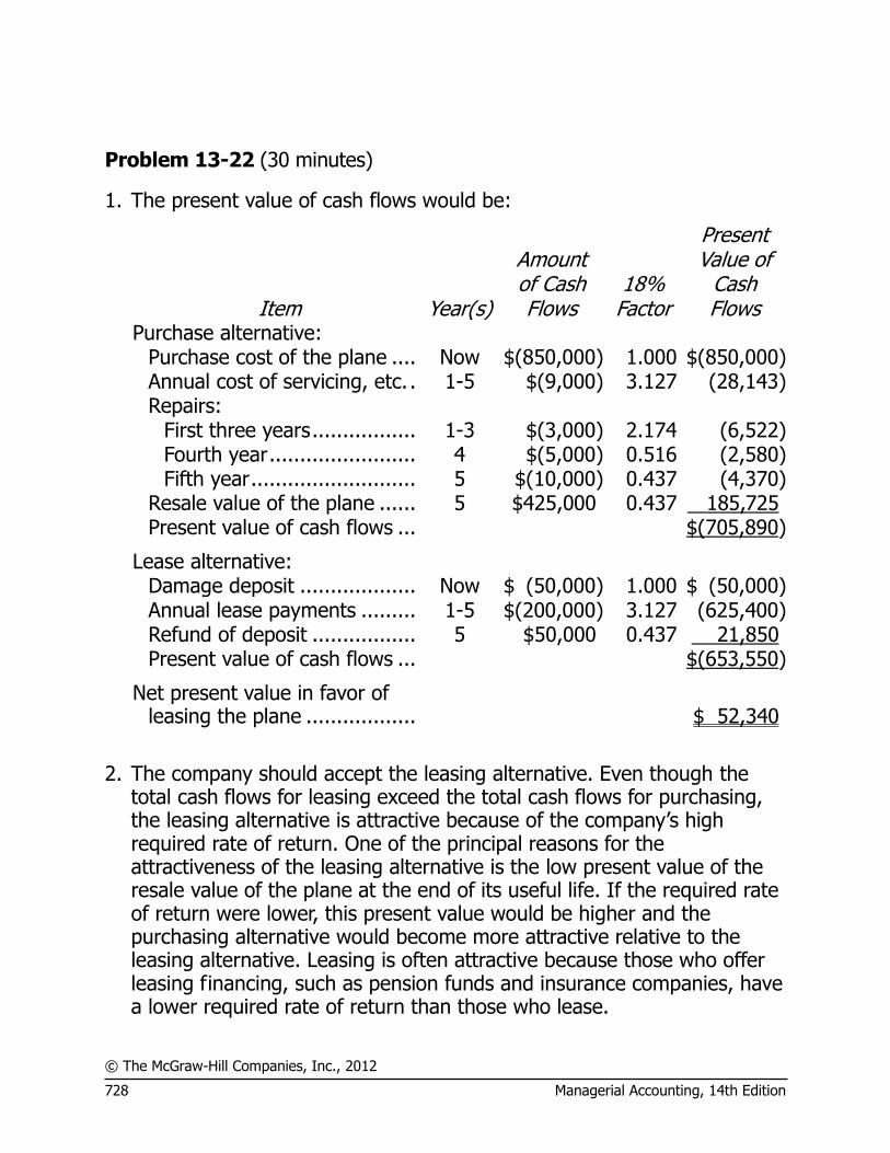
© The McGraw-Hill Companies, Inc., 2012
728 Managerial Accounting, 14th Edition
Problem 13-22 (30 minutes)
1. The present value of cash flows would be:
Item Year(s)
Amount of Cash Flows
18% Factor
Present Value of
Cash Flows
Purchase alternative: Purchase cost of the plane .... Now $(850,000) 1.000 $(850,000) Annual cost of servicing, etc. . 1-5 $(9,000) 3.127 (28,143) Repairs:
First three years ................. 1-3 $(3,000) 2.174 (6,522) Fourth year ........................ 4 $(5,000) 0.516 (2,580) Fifth year ........................... 5 $(10,000) 0.437 (4,370)
Resale value of the plane ...... 5 $425,000 0.437 185,725 Present value of cash flows ... $(705,890)
Lease alternative: Damage deposit ................... Now $ (50,000) 1.000 $ (50,000) Annual lease payments ......... 1-5 $(200,000) 3.127 (625,400) Refund of deposit ................. 5 $50,000 0.437 21,850 Present value of cash flows ... $(653,550)
Net present value in favor of leasing the plane .................. $ 52,340
2. The company should accept the leasing alternative. Even though the
total cash flows for leasing exceed the total cash flows for purchasing, the leasing alternative is attractive because of the company’s high required rate of return. One of the principal reasons for the attractiveness of the leasing alternative is the low present value of the resale value of the plane at the end of its useful life. If the required rate of return were lower, this present value would be higher and the purchasing alternative would become more attractive relative to the leasing alternative. Leasing is often attractive because those who offer leasing financing, such as pension funds and insurance companies, have a lower required rate of return than those who lease.
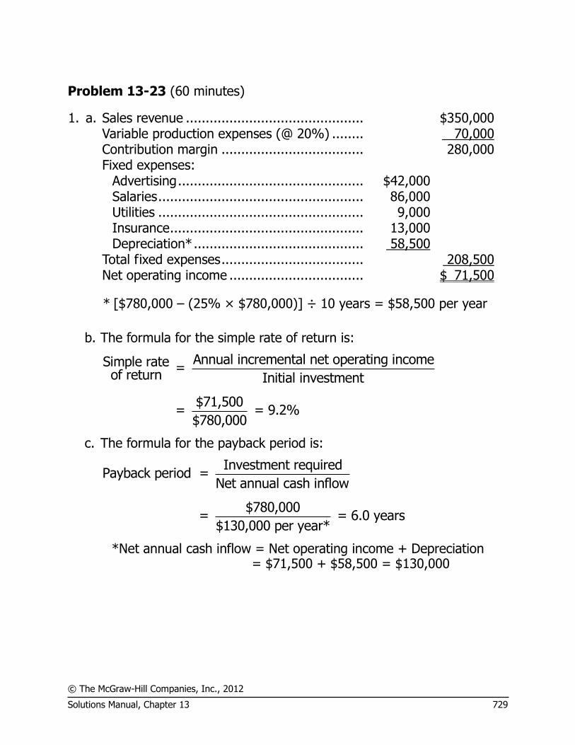
© The McGraw-Hill Companies, Inc., 2012
Solutions Manual, Chapter 13 729
Problem 13-23 (60 minutes)
1. a. Sales revenue ............................................. $350,000 Variable production expenses (@ 20%) ........ 70,000 Contribution margin .................................... 280,000 Fixed expenses: Advertising ............................................... $42,000 Salaries .................................................... 86,000 Utilities .................................................... 9,000 Insurance ................................................. 13,000 Depreciation* ........................................... 58,500 Total fixed expenses .................................... 208,500 Net operating income .................................. $ 71,500
* [$780,000 – (25% × $780,000)] ÷ 10 years = $58,500 per year
b. The formula for the simple rate of return is:
Annual incremental net operating incomeSimple rate = of return Initial investment
$71,500= = 9.2%
$780,000
c. The formula for the payback period is:
Investment requiredPayback period =
Net annual cash inflow
$780,000= = 6.0 years
$130,000 per year*
*Net annual cash inflow = Net operating income + Depreciation = $71,500 + $58,500 = $130,000

© The McGraw-Hill Companies, Inc., 2012
730 Managerial Accounting, 14th Edition
Problem 13-23 (continued)
2. a. A cost reduction project is involved here, so the formula for the simple rate of return would be:
Cost savings - Depreciation
Simple rate of return = Initial Salvage from -
investment old equipment
The reduction in costs with the new equipment would be:
Annual costs, old equipment ................ $85,000 Annual costs, new equipment:
Salary of operator ............................. $26,000 Maintenance ..................................... 3,000 29,000
Annual savings in costs ........................ $56,000
Thus, the simple rate of return would be:
$56,000 - $22,000* $34,000
= = 16.0%$220,000 - $7,200 $212,800
*$220,000 ÷ 10 years = $22,000 per year b. The formula for the payback period remains the same as in Part (1),
except we must reduce the investment required by the salvage from sale of the old equipment:
Investment Salvage from - required old equipment
Payback period = Net annual cash inflow
$220,000 - $7,200= = 3.8 years
$56,000 per year*
*See Part (2a) above. 3. According to the company’s criteria, machine A should not be purchased
and machine B should be purchased.
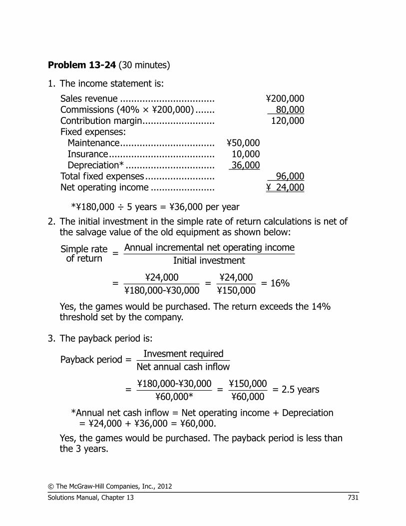
© The McGraw-Hill Companies, Inc., 2012
Solutions Manual, Chapter 13 731
Problem 13-24 (30 minutes)
1. The income statement is:
Sales revenue .................................. ¥200,000 Commissions (40% × ¥200,000) ....... 80,000 Contribution margin .......................... 120,000 Fixed expenses:
Maintenance .................................. ¥50,000 Insurance ...................................... 10,000 Depreciation* ................................ 36,000
Total fixed expenses ......................... 96,000 Net operating income ....................... ¥ 24,000
*¥180,000 ÷ 5 years = ¥36,000 per year
2. The initial investment in the simple rate of return calculations is net of the salvage value of the old equipment as shown below:
Annual incremental net operating incomeSimple rate = of return Initial investment
¥24,000 ¥24,000= = = 16%
¥180,000-¥30,000 ¥150,000
Yes, the games would be purchased. The return exceeds the 14% threshold set by the company.
3. The payback period is:
Invesment requiredPayback period =
Net annual cash inflow
¥180,000-¥30,000 ¥150,000= = = 2.5 years
¥60,000* ¥60,000
*Annual net cash inflow = Net operating income + Depreciation = ¥24,000 + ¥36,000 = ¥60,000.
Yes, the games would be purchased. The payback period is less than the 3 years.

© The McGraw-Hill Companies, Inc., 2012
732 Managerial Accounting, 14th Edition
Problem 13-25 (30 minutes)
1. The total-cost approach:
Year(s)
Amount of Cash Flows
16% Factor
Present Value of
Cash Flows
Purchase the new generator: Cost of the new generator ....... Now $(20,000) 1.000 $(20,000) Salvage of the old generator .... Now $4,000 1.000 4,000 Annual cash operating costs .... 1-8 $(7,500) 4.344 (32,580) Salvage of the new generator .. 8 $6,000 0.305 1,830 Present value of the net cash
outflows ............................... $(46,750)
Keep the old generator: Overhaul needed now .............. Now $(8,000) 1.000 $ (8,000) Annual cash operating costs ..... 1-8 $(12,500) 4.344 (54,300) Salvage of the old generator ..... 8 $3,000 0.305 915 Present value of the net cash
outflows ............................... $(61,385)
Net present value in favor of purchasing the new generator .. $ 14,635
The hospital should purchase the new generator because it has the
lowest present value of total cost.

© The McGraw-Hill Companies, Inc., 2012
Solutions Manual, Chapter 13 733
Problem 13-25 (continued)
2. The incremental-cost approach:
Year(s)
Amount of Cash Flows
16% Factor
Present Value of
Cash Flows
Incremental investment—new
generator* ............................. Now $(12,000) 1.000 $(12,000) Salvage of the old generator ...... Now $4,000 1.000 4,000 Savings in annual cash operating
costs ...................................... 1-8 $5,000 4.344 21,720 Difference in salvage value in 8
years ...................................... 8 $3,000 0.305 915 Net present value in favor of
purchasing the new generator . $ 14,635
*$20,000 – $8,000 = $12,000.
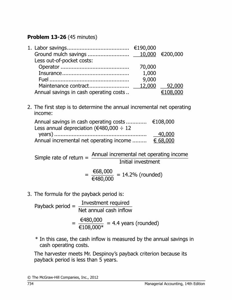
© The McGraw-Hill Companies, Inc., 2012
734 Managerial Accounting, 14th Edition
Problem 13-26 (45 minutes)
1. Labor savings ....................................... €190,000 Ground mulch savings .......................... 10,000 €200,000 Less out-of-pocket costs: Operator ........................................... 70,000 Insurance .......................................... 1,000 Fuel .................................................. 9,000 Maintenance contract ......................... 12,000 92,000 Annual savings in cash operating costs .. €108,000
2. The first step is to determine the annual incremental net operating
income:
Annual savings in cash operating costs ............. €108,000
Less annual depreciation (€480,000 ÷ 12
years) .......................................................... 40,000 Annual incremental net operating income ......... € 68,000
Annual incremental net operating incomeSimple rate of return =
Initial investment
€68,000= = 14.2% (rounded)
€480,000
3. The formula for the payback period is:
Investment requiredPayback period =
Net annual cash inflow
€480,000= = 4.4 years (rounded)
€108,000*
* In this case, the cash inflow is measured by the annual savings in cash operating costs.
The harvester meets Mr. Despinoy’s payback criterion because its payback period is less than 5 years.

© The McGraw-Hill Companies, Inc., 2012
Solutions Manual, Chapter 13 735
Problem 13-26 (continued)
4. The formula for the internal rate of return is:
Investment requiredFactor of the internal = rate of return Net annual cash inflow
€480,000= = 4.4 (rounded)
€108,000
Looking at Exhibit 13B-2 in Appendix 13B, and reading along the 12-period line, a factor of 4.4 would represent an internal rate of return of approximately 20%.
Note that the payback and internal rate of return methods would indicate that the investment should be made. The simple rate of return method indicates the opposite since the simple rate of return is less than 16%. The simple rate of return method generally is not an accurate guide in investment decisions.
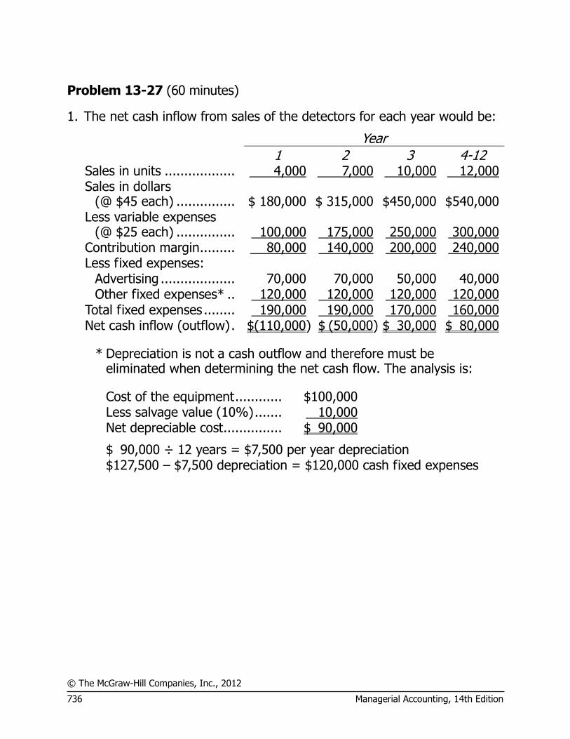
© The McGraw-Hill Companies, Inc., 2012
736 Managerial Accounting, 14th Edition
Problem 13-27 (60 minutes)
1. The net cash inflow from sales of the detectors for each year would be:
Year 1 2 3 4-12 Sales in units .................. 4,000 7,000 10,000 12,000 Sales in dollars
(@ $45 each) ............... $ 180,000 $ 315,000 $450,000 $540,000 Less variable expenses
(@ $25 each) ............... 100,000 175,000 250,000 300,000 Contribution margin ......... 80,000 140,000 200,000 240,000 Less fixed expenses:
Advertising ................... 70,000 70,000 50,000 40,000 Other fixed expenses* .. 120,000 120,000 120,000 120,000
Total fixed expenses ........ 190,000 190,000 170,000 160,000 Net cash inflow (outflow) . $(110,000) $ (50,000) $ 30,000 $ 80,000
* Depreciation is not a cash outflow and therefore must be eliminated when determining the net cash flow. The analysis is:
Cost of the equipment ............ $100,000 Less salvage value (10%) ....... 10,000 Net depreciable cost ............... $ 90,000
$ 90,000 ÷ 12 years = $7,500 per year depreciation $127,500 – $7,500 depreciation = $120,000 cash fixed expenses

© The McGraw-Hill Companies, Inc., 2012
Solutions Manual, Chapter 13 737
Problem 13-27 (continued)
2. The net present value of the proposed investment would be:
Item Year(s)
Amount of Cash Flows
20% Factor
Present Value of
Cash Flows
Investment in equipment ... Now $(100,000) 1.000 $(100,000) Working capital investment Now $(40,000) 1.000 (40,000) Yearly cash flows ............... 1 $(110,000) 0.833 (91,630) " " " ................ 2 $(50,000) 0.694 (34,700) " " " ................ 3 $30,000 0.579 17,370 " " " ................ 4-12 $80,000 2.333 * 186,640 Salvage value of
equipment ...................... 12 $10,000 0.112 1,120 Release of working capital . 12 $40,000 0.112 4,480 Net present value .............. $ (56,720)
* Present value factor for 12 periods ...................... 4.439 Present value factor for 3 periods ........................ 2.106
Present value factor for 9 periods, starting 4
periods in the future ........................................ 2.333
Since the net present value is negative, the company should not accept the smoke detector as a new product.
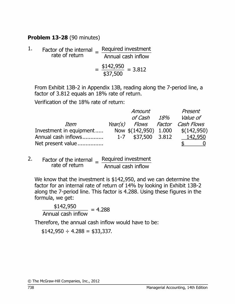
© The McGraw-Hill Companies, Inc., 2012
738 Managerial Accounting, 14th Edition
Problem 13-28 (90 minutes)
1. Required investmentFactor of the internal = rate of return Annual cash inflow
$142,950= = 3.812
$37,500
From Exhibit 13B-2 in Appendix 13B, reading along the 7-period line, a
factor of 3.812 equals an 18% rate of return.
Verification of the 18% rate of return:
Item Year(s)
Amount of Cash Flows
18% Factor
Present Value of
Cash Flows Investment in equipment ..... Now $(142,950) 1.000 $(142,950) Annual cash inflows ............. 1-7 $37,500 3.812 142,950 Net present value ................ $ 0
2. Required investmentFactor of the internal =
rate of return Annual cash inflow
We know that the investment is $142,950, and we can determine the
factor for an internal rate of return of 14% by looking in Exhibit 13B-2 along the 7-period line. This factor is 4.288. Using these figures in the formula, we get:
$142,950
= 4.288Annual cash inflow
Therefore, the annual cash inflow would have to be:
$142,950 ÷ 4.288 = $33,337.

© The McGraw-Hill Companies, Inc., 2012
Solutions Manual, Chapter 13 739
Problem 13-28 (continued)
3. a. 5-year life for the equipment: The factor for the internal rate of return would still be 3.812 [as
computed in (1) above]. From Exhibit 13B-2, reading this time along the 5-period line, a factor of 3.812 is closest to 3.791, the factor for 10%. Thus, to the nearest whole percent, the internal rate of return is 10%.
b. 9-year life for the equipment: The factor of the internal rate of return would again be 3.812. From
Exhibit 13B-2, reading along the 9-period line, a factor of 3.812 is closest to 3.786, the factor for 22%. Thus, to the nearest whole percent, the internal rate of return is 22%.
The 10% return in part (a) is less than the 14% minimum return that Dr. Black wants to earn on the project. Of equal or even greater importance, the following diagram should be pointed out to Dr. Black:
2 years shorter 2 years longer 5
years 10%
7 years 18%
9 years 22%
A reduction of 8% An increase of only 4% As this illustration shows, a decrease in years has a much greater
impact on the rate of return than an increase in years. This is because of the time value of money; added cash inflows far into the future do little to enhance the rate of return, but loss of cash inflows in the near term can do much to reduce it. Therefore, Dr. Black should be very concerned about any potential decrease in the life of the equipment, while at the same time realizing that any increase in the life of the equipment will do little to enhance her rate of return.

© The McGraw-Hill Companies, Inc., 2012
740 Managerial Accounting, 14th Edition
Problem 13-28 (continued)
4. a. The expected annual cash inflow would be:
$37,500 × 120% = $45,000
$142,950 = 3.177
$45,000
From Exhibit 13B-2 in Appendix 13B, reading along the 7-period line, a factor of 3.177 is closest to 3.161, the factor for 25%, and is between that factor and the factor for 24%. Thus, to the nearest whole percent, the internal rate of return is 25%.
b. The expected annual cash inflow would be:
$37,500 × 80% = $30,000
$142,950 = 4.765
$30,000
From Exhibit 13B-2 in Appendix 13B, reading along the 7-period line, a factor of 4.765 is closest to 4.712, the factor for 11%. Thus, to the nearest whole percent, the internal rate of return is 11%.
Unlike changes in time, increases and decreases in cash flows at a
given point in time have basically the same impact on the rate of return, as shown below:
20% decrease
in cash flow 20% increase in
cash flow
$30,000 cash inflow
11%
$37,500 cash inflow
18%
$45,000 cash inflow
25% A decrease of
7% An increase of
7%

© The McGraw-Hill Companies, Inc., 2012
Solutions Manual, Chapter 13 741
Problem 13-28 (continued)
5. The cash flows are not even over the five-year period (there is an extra $61,375 cash inflow from sale of the equipment at the end of the fifth year), so the formula method cannot be used to compute the internal rate of return. Using trial-and-error or more sophisticated methods, it turns out that the actual internal rate of return will be 12%:
Item Year(s)
Amount of Cash Flows
12% Factor
Present Value of
Cash Flows Investment in the equipment . Now $(142,950) 1.000 $(142,950) Annual cash inflow ................ 1-5 $30,000 3.605 108,150 Sale of the equipment ........... 5 $61,375 0.567 34,800 Net present value .................. $ 0
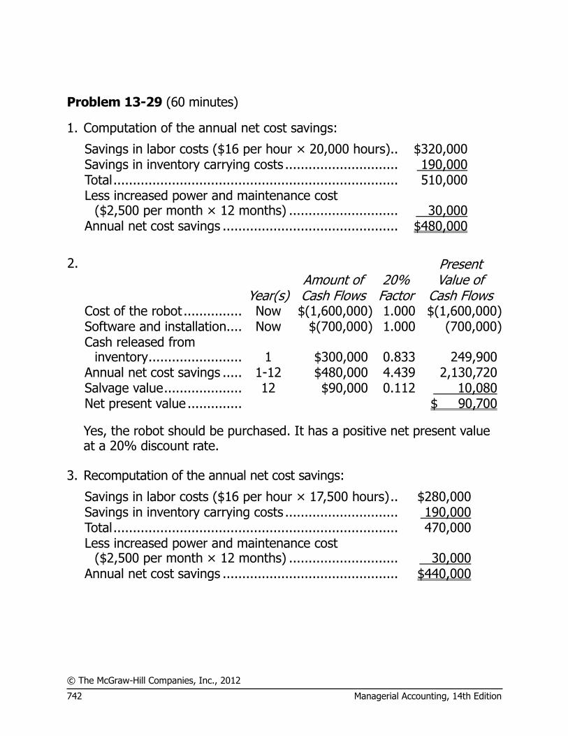
© The McGraw-Hill Companies, Inc., 2012
742 Managerial Accounting, 14th Edition
Problem 13-29 (60 minutes)
1. Computation of the annual net cost savings:
Savings in labor costs ($16 per hour × 20,000 hours) .. $320,000 Savings in inventory carrying costs ............................. 190,000 Total ......................................................................... 510,000 Less increased power and maintenance cost
($2,500 per month × 12 months) ............................ 30,000 Annual net cost savings ............................................. $480,000
2.
Year(s) Amount of Cash Flows
20% Factor
Present Value of
Cash Flows Cost of the robot ............... Now $(1,600,000) 1.000 $(1,600,000) Software and installation.... Now $(700,000) 1.000 (700,000)
Cash released from
inventory ........................ 1 $300,000 0.833 249,900 Annual net cost savings ..... 1-12 $480,000 4.439 2,130,720 Salvage value .................... 12 $90,000 0.112 10,080 Net present value .............. $ 90,700
Yes, the robot should be purchased. It has a positive net present value at a 20% discount rate.
3. Recomputation of the annual net cost savings:
Savings in labor costs ($16 per hour × 17,500 hours) .. $280,000 Savings in inventory carrying costs ............................. 190,000 Total ......................................................................... 470,000 Less increased power and maintenance cost
($2,500 per month × 12 months) ............................ 30,000 Annual net cost savings ............................................. $440,000
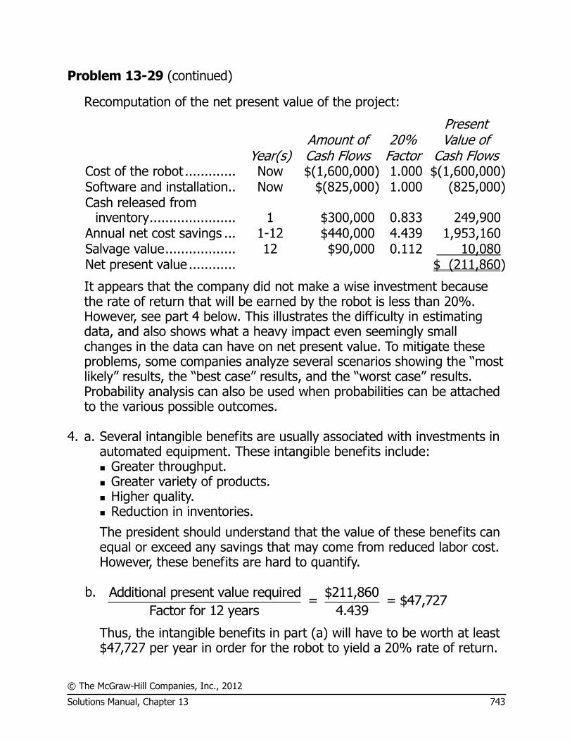
© The McGraw-Hill Companies, Inc., 2012
Solutions Manual, Chapter 13 743
Problem 13-29 (continued)
Recomputation of the net present value of the project:
Year(s) Amount of Cash Flows
20% Factor
Present Value of
Cash Flows Cost of the robot ............. Now $(1,600,000) 1.000 $(1,600,000) Software and installation.. Now $(825,000) 1.000 (825,000)
Cash released from
inventory ...................... 1 $300,000 0.833 249,900 Annual net cost savings ... 1-12 $440,000 4.439 1,953,160 Salvage value .................. 12 $90,000 0.112 10,080 Net present value ............ $ (211,860)
It appears that the company did not make a wise investment because the rate of return that will be earned by the robot is less than 20%. However, see part 4 below. This illustrates the difficulty in estimating data, and also shows what a heavy impact even seemingly small changes in the data can have on net present value. To mitigate these problems, some companies analyze several scenarios showing the “most likely” results, the “best case” results, and the “worst case” results. Probability analysis can also be used when probabilities can be attached to the various possible outcomes.
4. a. Several intangible benefits are usually associated with investments in
automated equipment. These intangible benefits include: Greater throughput. Greater variety of products. Higher quality. Reduction in inventories.
The president should understand that the value of these benefits can equal or exceed any savings that may come from reduced labor cost. However, these benefits are hard to quantify.
b. Additional present value required $211,860
= = $47,727Factor for 12 years 4.439
Thus, the intangible benefits in part (a) will have to be worth at least $47,727 per year in order for the robot to yield a 20% rate of return.
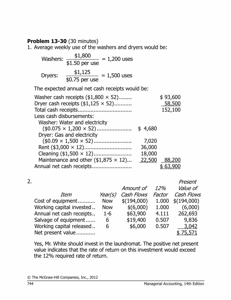
© The McGraw-Hill Companies, Inc., 2012
744 Managerial Accounting, 14th Edition
Problem 13-30 (30 minutes) 1. Average weekly use of the washers and dryers would be:
$1,800Washers: = 1,200 uses
$1.50 per use
$1,125Dryers: = 1,500 uses
$0.75 per use
The expected annual net cash receipts would be:
Washer cash receipts ($1,800 × 52) ........ $ 93,600 Dryer cash receipts ($1,125 × 52) ........... 58,500
Total cash receipts .................................. 152,100 Less cash disbursements:
Washer: Water and electricity ($0.075 × 1,200 × 52) ...................... $ 4,680
Dryer: Gas and electricity ($0.09 × 1,500 × 52) ........................ 7,020
Rent ($3,000 × 12) .............................. 36,000 Cleaning ($1,500 × 12) ........................ 18,000 Maintenance and other ($1,875 × 12) ... 22,500 88,200
Annual net cash receipts ......................... $ 63,900
2.
Item Year(s) Amount of Cash Flows
12% Factor
Present Value of
Cash Flows Cost of equipment ........... Now $(194,000) 1.000 $(194,000) Working capital invested .. Now $(6,000) 1.000 (6,000) Annual net cash receipts .. 1-6 $63,900 4.111 262,693 Salvage of equipment ...... 6 $19,400 0.507 9,836 Working capital released .. 6 $6,000 0.507 3,042 Net present value ............ $ 75,571
Yes, Mr. White should invest in the laundromat. The positive net present value indicates that the rate of return on this investment would exceed the 12% required rate of return.

© The McGraw-Hill Companies, Inc., 2012
Solutions Manual, Chapter 13 745
Problem 13-31 (45 minutes)
1. A net present value computation for each investment follows:
Item Year(s) Amount of Cash Flows
20% Factor
Present Value of
Cash Flows Common stock:
Purchase of the stock ........ Now $(80,000) 1.000 $(80,000) Sale of the stock ............... 4 $180,000 0.482 86,760 Net present value .............. $ 6,760
Preferred stock: Purchase of the stock ........ Now $(30,000) 1.000 $(30,000) Annual cash dividend
(6%).............................. 1-4 $1,800 2.589 4,660 Sale of the stock ............... 4 $24,000 0.482 11,568 Net present value .............. $(13,772)
Bonds: Purchase of the bonds ....... Now $(50,000) 1.000 $(50,000) Semiannual interest
received ......................... 1-8* $3,000 5.335** 16,005 Sale of the bonds .............. 8* $58,500 0.467** 27,320 Net present value .............. $ (6,675)
* 8 semiannual interest periods. ** Factor for 8 periods at 10%.
Anita earned a 20% rate of return on the common stock, but not on the
preferred stock or the bonds.

© The McGraw-Hill Companies, Inc., 2012
746 Managerial Accounting, 14th Edition
Problem 13-31 (continued)
2. Considering all three investments together, Anita did not earn a 20% rate of return. The computation is:
Net Present Value
Common stock ........................ $ 6,760 Preferred stock ........................ (13,772) Bonds ..................................... (6,675) Overall net present value ......... $(13,687)
The defect in the broker’s computation is that it does not consider the time value of money and therefore has overstated the rate of return earned.
3. Because the assumption is that the project will yield the same annual
cash inflow every year, the formula for the net present value of the project is:
Net present Present value AnnualInvestmentvalue of = factor for × cash -
requiredthe project an annuity inflow
Substituting the $262,500 investment and the factor for 16% for 10 periods into this formula and requiring that the net present value be positive, we get:
4.833 × Annual cash inflow – $262,500 > 0
Therefore, the required annual net cash inflow is at least:
Annual cash inflow > $262,500 ÷ 4.833 = $54,314

© The McGraw-Hill Companies, Inc., 2012
Solutions Manual, Chapter 13 747
Problem 13-32 (45 minutes)
The annual net cash inflow from rental of the property would be:
Net operating income .......... $30,100 Add back depreciation ......... 17,800 Annual net cash inflow ........ $47,900
Given this figure, the present value analysis would be as follows:
Item Year(s)
Amount of Cash Flows
14% Factor
Present Value of
Cash Flows
Keep the property: Annual loan payment ...... 1-10 $(12,600) 5.216 $ (65,722) Annual net cash inflow .... 1-16 $47,900 6.265 300,094
Resale value of the
property ...................... 16 $139,600 * 0.123 17,171
Present value of cash
flows ........................... $251,543
Sell the property: Payoff of mortgage ......... Now $(71,000) 1.000 $ (71,000) Down payment received .. Now $150,000 1.000 150,000
Annual payments
received ...................... 1-16 $23,000 6.265 144,095
Present value of cash
flows ........................... $223,095
Net present value in favor
of keeping the property ... $ 28,448
*Land: $52,000 × 2.5 = $130,000; Building: $9,600; Total: $139,600.
Thus, Professor Ryatt should be advised to keep the property. Note that even if the property were worth nothing at the end of 16 years, it would still be more desirable to keep the property rather than sell it under the terms offered by the realty company.
© The McGraw-Hill Companies, Inc., 2012
748 Managerial Accounting, 14th Edition
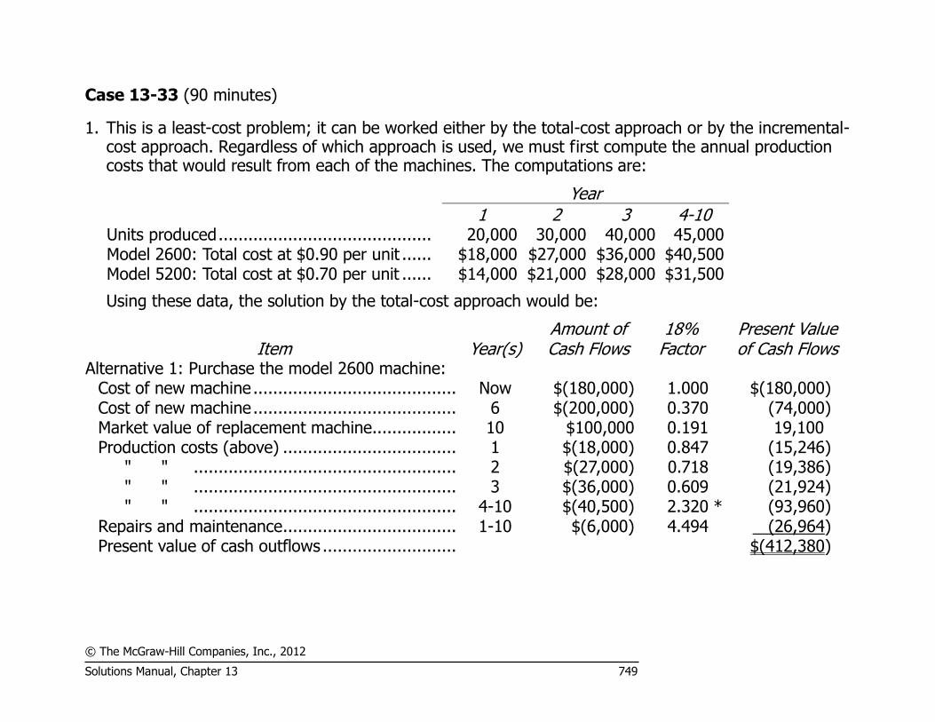
© The McGraw-Hill Companies, Inc., 2012
Solutions Manual, Chapter 13 749
Case 13-33 (90 minutes)
1. This is a least-cost problem; it can be worked either by the total-cost approach or by the incremental-cost approach. Regardless of which approach is used, we must first compute the annual production costs that would result from each of the machines. The computations are:
Year 1 2 3 4-10 Units produced ........................................... 20,000 30,000 40,000 45,000 Model 2600: Total cost at $0.90 per unit ...... $18,000 $27,000 $36,000 $40,500 Model 5200: Total cost at $0.70 per unit ...... $14,000 $21,000 $28,000 $31,500
Using these data, the solution by the total-cost approach would be:
Item Year(s) Amount of Cash Flows
18% Factor
Present Value of Cash Flows
Alternative 1: Purchase the model 2600 machine: Cost of new machine ......................................... Now $(180,000) 1.000 $(180,000) Cost of new machine ......................................... 6 $(200,000) 0.370 (74,000) Market value of replacement machine................. 10 $100,000 0.191 19,100 Production costs (above) ................................... 1 $(18,000) 0.847 (15,246)
" " ..................................................... 2 $(27,000) 0.718 (19,386) " " ..................................................... 3 $(36,000) 0.609 (21,924) " " ..................................................... 4-10 $(40,500) 2.320 * (93,960)
Repairs and maintenance ................................... 1-10 $(6,000) 4.494 (26,964) Present value of cash outflows ........................... $(412,380)
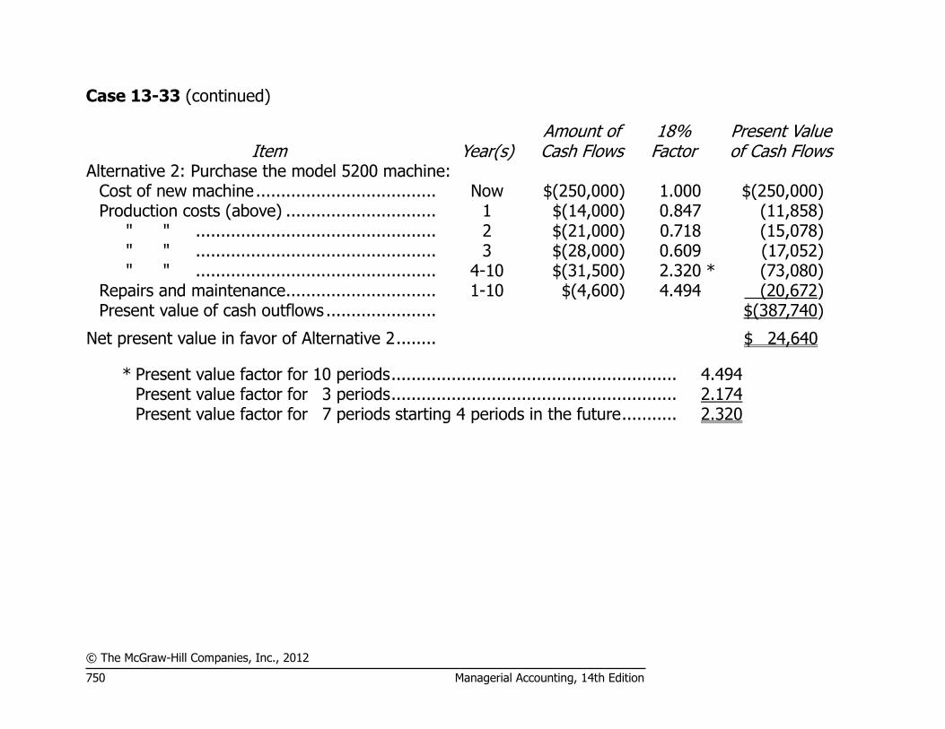
© The McGraw-Hill Companies, Inc., 2012
750 Managerial Accounting, 14th Edition
Case 13-33 (continued)
Item Year(s) Amount of Cash Flows
18% Factor
Present Value of Cash Flows
Alternative 2: Purchase the model 5200 machine: Cost of new machine .................................... Now $(250,000) 1.000 $(250,000) Production costs (above) .............................. 1 $(14,000) 0.847 (11,858)
" " ................................................ 2 $(21,000) 0.718 (15,078) " " ................................................ 3 $(28,000) 0.609 (17,052) " " ................................................ 4-10 $(31,500) 2.320 * (73,080)
Repairs and maintenance .............................. 1-10 $(4,600) 4.494 (20,672) Present value of cash outflows ...................... $(387,740)
Net present value in favor of Alternative 2 ........ $ 24,640
* Present value factor for 10 periods ......................................................... 4.494 Present value factor for 3 periods ......................................................... 2.174 Present value factor for 7 periods starting 4 periods in the future ........... 2.320
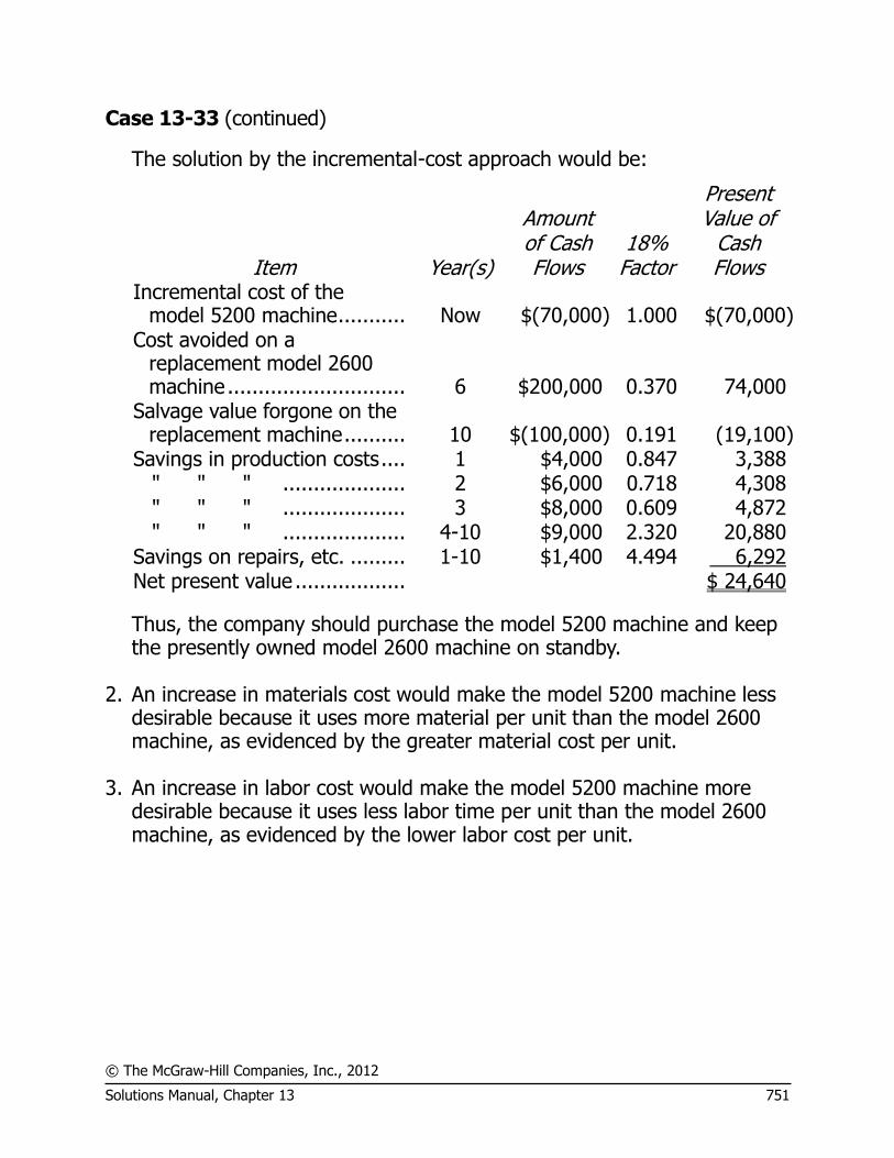
© The McGraw-Hill Companies, Inc., 2012
Solutions Manual, Chapter 13 751
Case 13-33 (continued)
The solution by the incremental-cost approach would be:
Item Year(s)
Amount of Cash Flows
18% Factor
Present Value of
Cash Flows
Incremental cost of the model 5200 machine ........... Now $(70,000) 1.000 $(70,000)
Cost avoided on a replacement model 2600 machine ............................. 6 $200,000 0.370 74,000
Salvage value forgone on the replacement machine .......... 10 $(100,000) 0.191 (19,100)
Savings in production costs .... 1 $4,000 0.847 3,388 " " " .................... 2 $6,000 0.718 4,308 " " " .................... 3 $8,000 0.609 4,872 " " " .................... 4-10 $9,000 2.320 20,880 Savings on repairs, etc. ......... 1-10 $1,400 4.494 6,292 Net present value .................. $ 24,640
Thus, the company should purchase the model 5200 machine and keep the presently owned model 2600 machine on standby.
2. An increase in materials cost would make the model 5200 machine less
desirable because it uses more material per unit than the model 2600 machine, as evidenced by the greater material cost per unit.
3. An increase in labor cost would make the model 5200 machine more
desirable because it uses less labor time per unit than the model 2600 machine, as evidenced by the lower labor cost per unit.
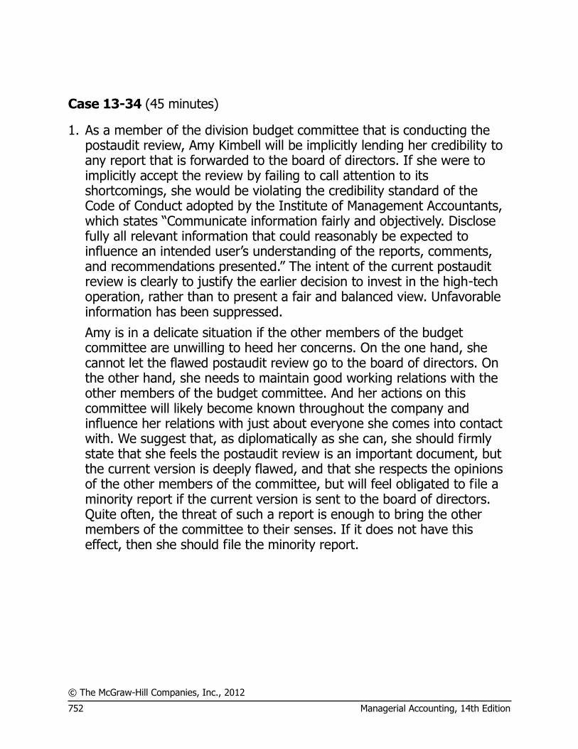
© The McGraw-Hill Companies, Inc., 2012
752 Managerial Accounting, 14th Edition
Case 13-34 (45 minutes)
1. As a member of the division budget committee that is conducting the postaudit review, Amy Kimbell will be implicitly lending her credibility to any report that is forwarded to the board of directors. If she were to implicitly accept the review by failing to call attention to its shortcomings, she would be violating the credibility standard of the Code of Conduct adopted by the Institute of Management Accountants, which states “Communicate information fairly and objectively. Disclose fully all relevant information that could reasonably be expected to influence an intended user’s understanding of the reports, comments, and recommendations presented.” The intent of the current postaudit review is clearly to justify the earlier decision to invest in the high-tech operation, rather than to present a fair and balanced view. Unfavorable information has been suppressed.
Amy is in a delicate situation if the other members of the budget committee are unwilling to heed her concerns. On the one hand, she cannot let the flawed postaudit review go to the board of directors. On the other hand, she needs to maintain good working relations with the other members of the budget committee. And her actions on this committee will likely become known throughout the company and influence her relations with just about everyone she comes into contact with. We suggest that, as diplomatically as she can, she should firmly state that she feels the postaudit review is an important document, but the current version is deeply flawed, and that she respects the opinions of the other members of the committee, but will feel obligated to file a minority report if the current version is sent to the board of directors. Quite often, the threat of such a report is enough to bring the other members of the committee to their senses. If it does not have this effect, then she should file the minority report.

© The McGraw-Hill Companies, Inc., 2012
Solutions Manual, Chapter 13 753
Case 13-34 (continued)
2. Unfortunately, the situation that Amy faces is all too common. Rather than acknowledge mistakes and cut losses, managers (and people in general) too often remain committed to their failing courses of action. This commitment leads people into self-delusion, self-justification, and cover-ups—all of which sap time and energy as well as perpetuating the results of bad decisions. Postaudits, if conducted properly, provide an escape route from this self-defeating behavior.
The review process is flawed from the very beginning if the postaudit review is prepared by the same people who approved the original proposal. The people who approved the original proposal are probably going to be interested in justifying their original decision rather than in conducting an objective review. Therefore, the postaudit review should be conducted by an independent group—perhaps the company’s internal audit office—rather than by the division budget committees.
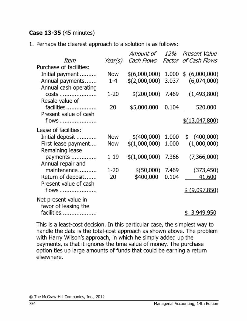
© The McGraw-Hill Companies, Inc., 2012
754 Managerial Accounting, 14th Edition
Case 13-35 (45 minutes)
1. Perhaps the clearest approach to a solution is as follows:
Item Year(s)
Amount of Cash Flows
12% Factor
Present Value of Cash Flows
Purchase of facilities: Initial payment .......... Now $(6,000,000) 1.000 $ (6,000,000) Annual payments ....... 1-4 $(2,000,000) 3.037 (6,074,000) Annual cash operating
costs ...................... 1-20 $(200,000) 7.469 (1,493,800) Resale value of
facilities .................. 20 $5,000,000 0.104 520,000 Present value of cash
flows ...................... $(13,047,800)
Lease of facilities: Initial deposit ............ Now $(400,000) 1.000 $ (400,000) First lease payment .... Now $(1,000,000) 1.000 (1,000,000) Remaining lease
payments ............... 1-19 $(1,000,000) 7.366 (7,366,000) Annual repair and
maintenance ........... 1-20 $(50,000) 7.469 (373,450) Return of deposit ....... 20 $400,000 0.104 41,600 Present value of cash
flows ...................... $ (9,097,850)
Net present value in favor of leasing the facilities ..................... $ 3,949,950
This is a least-cost decision. In this particular case, the simplest way to handle the data is the total-cost approach as shown above. The problem with Harry Wilson’s approach, in which he simply added up the payments, is that it ignores the time value of money. The purchase option ties up large amounts of funds that could be earning a return elsewhere.
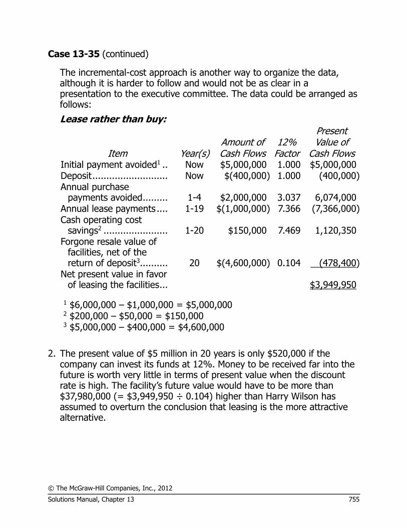
© The McGraw-Hill Companies, Inc., 2012
Solutions Manual, Chapter 13 755
Case 13-35 (continued)
The incremental-cost approach is another way to organize the data, although it is harder to follow and would not be as clear in a presentation to the executive committee. The data could be arranged as follows:
Lease rather than buy:
Item Year(s) Amount of Cash Flows
12% Factor
Present Value of
Cash Flows Initial payment avoided1 .. Now $5,000,000 1.000 $5,000,000 Deposit ........................... Now $(400,000) 1.000 (400,000) Annual purchase
payments avoided ......... 1-4 $2,000,000 3.037 6,074,000 Annual lease payments .... 1-19 $(1,000,000) 7.366 (7,366,000) Cash operating cost
savings2 ....................... 1-20 $150,000 7.469 1,120,350 Forgone resale value of
facilities, net of the return of deposit3 .......... 20 $(4,600,000) 0.104 (478,400)
Net present value in favor of leasing the facilities ... $3,949,950
1 $6,000,000 – $1,000,000 = $5,000,000 2 $200,000 – $50,000 = $150,000 3 $5,000,000 – $400,000 = $4,600,000
2. The present value of $5 million in 20 years is only $520,000 if the
company can invest its funds at 12%. Money to be received far into the future is worth very little in terms of present value when the discount rate is high. The facility’s future value would have to be more than $37,980,000 (= $3,949,950 ÷ 0.104) higher than Harry Wilson has assumed to overturn the conclusion that leasing is the more attractive alternative.

© The McGraw-Hill Companies, Inc., 2012
756 Managerial Accounting, 14th Edition
Appendix 13A The Concept of Present Value
Exercise 13A-1 (10 minutes)
a. From Exhibit 13B-1, the present value factor for 8% for three periods is 0.794. Therefore, the present value of the investment in the garage is $317,600 (=$400,000 × 0.794). If $317,600 is invested now at 8%, in three years it will have grown to $400,000.
b. From Exhibit 13B-1, the present value factor for 12% for three periods
is 0.712. Therefore, the present value of the investment in the garage is $284,800 (=$400,000 × 0.712). If $284,800 is invested now at 12%, in three years it will have grown to $400,000.
Exercise 13A-2 (10 minutes)
You should prefer option (a) because its present value is the largest:
Option a: $50,000 × 1.000 = $50,000. Option b: $75,000 × 0.507 = $38,025. (From Exhibit 13B-1) Option c: $12,000 × 4.111 = $49,332. (From Exhibit 13B-2)
Exercise 13A-3 (10 minutes)
a. From Exhibit 13B-1, the factor for 6% for 3 periods is 0.840. Therefore, the present value of the required investment is:
$12,000 × 0.840 = $10,080.
b. From Exhibit 13B-1, the factor for 10% for 3 periods is 0.751. Therefore, the present value of the required investment is:
$12,000 × 0.751 = $9,012.
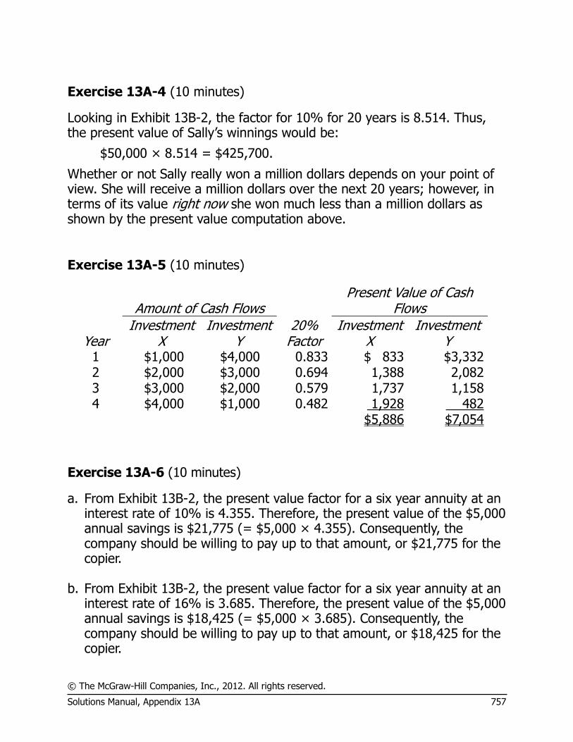
© The McGraw-Hill Companies, Inc., 2012. All rights reserved.
Solutions Manual, Appendix 13A 757
Exercise 13A-4 (10 minutes)
Looking in Exhibit 13B-2, the factor for 10% for 20 years is 8.514. Thus, the present value of Sally’s winnings would be:
$50,000 × 8.514 = $425,700.
Whether or not Sally really won a million dollars depends on your point of view. She will receive a million dollars over the next 20 years; however, in terms of its value right now she won much less than a million dollars as shown by the present value computation above.
Exercise 13A-5 (10 minutes)
Amount of Cash Flows Present Value of Cash
Flows
Year Investment
X Investment
Y 20%
Factor Investment
X Investment
Y 1 $1,000 $4,000 0.833 $ 833 $3,332 2 $2,000 $3,000 0.694 1,388 2,082 3 $3,000 $2,000 0.579 1,737 1,158 4 $4,000 $1,000 0.482 1,928 482 $5,886 $7,054
Exercise 13A-6 (10 minutes)
a. From Exhibit 13B-2, the present value factor for a six year annuity at an interest rate of 10% is 4.355. Therefore, the present value of the $5,000 annual savings is $21,775 (= $5,000 × 4.355). Consequently, the company should be willing to pay up to that amount, or $21,775 for the copier.
b. From Exhibit 13B-2, the present value factor for a six year annuity at an
interest rate of 16% is 3.685. Therefore, the present value of the $5,000 annual savings is $18,425 (= $5,000 × 3.685). Consequently, the company should be willing to pay up to that amount, or $18,425 for the copier.
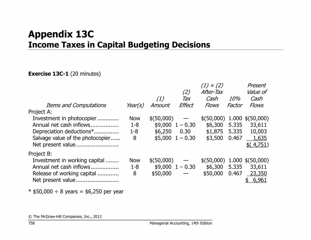
© The McGraw-Hill Companies, Inc., 2012
758 Managerial Accounting, 14th Edition
Appendix 13C Income Taxes in Capital Budgeting Decisions
Exercise 13C-1 (20 minutes)
Items and Computations Year(s) (1)
Amount
(2) Tax
Effect
(1) × (2) After-Tax
Cash Flows
10% Factor
Present Value of
Cash Flows
Project A: Investment in photocopier ............. Now $(50,000) — $(50,000) 1.000 $(50,000) Annual net cash inflows ................. 1-8 $9,000 1 – 0.30 $6,300 5.335 33,611 Depreciation deductions* ............... 1-8 $6,250 0.30 $1,875 5.335 10,003 Salvage value of the photocopier ...... 8 $5,000 1 – 0.30 $3,500 0.467 1,635 Net present value .......................... $( 4,751)
Project B: Investment in working capital ........ Now $(50,000) — $(50,000) 1.000 $(50,000) Annual net cash inflows ................. 1-8 $9,000 1 – 0.30 $6,300 5.335 33,611 Release of working capital ............. 8 $50,000 — $50,000 0.467 23,350 Net present value .......................... $ 6,961
* $50,000 ÷ 8 years = $6,250 per year

© The McGraw-Hill Companies, Inc., 2012. All rights reserved.
Solutions Manual, Appendix 13C 759
Exercise 13C-2 (20 minutes)
1. Annual cost of student help in collating ............ $60,000 Annual cost of the new collating machine: Operator ...................................................... $18,000 Maintenance ................................................ 7,000 25,000 Annual net cost savings (cash inflow) .............. $35,000
2. The net present value analysis follows:
Items and Computations Year(s) (1)
Amount
(2) Tax
Effect
(1) × (2) After-Tax
Cash Flows 14%
Factor
Present Value of
Cash Flows Cost of the new collating machine .... Now $(140,000) $(140,000) 1.000 $(140,000) Annual net cost savings (above) ....... 1-10 $35,000 1 – 0.30 $24,500 5.216 127,792 Depreciation deductions* ................. 1-10 $14,000 0.30 $4,200 5.216 21,907 Cost of the new roller pads ............... 5 $(20,000) 1 – 0.30 $(14,000) 0.519 (7,266) Salvage value of the new machine .... 10 $40,000 1 – 0.30 $28,000 0.270 7,560 Net present value ............................ $ 9,993
* $140,000 ÷ 10 years = $14,000 per year Yes, the new collating machine should be purchased.

© The McGraw-Hill Companies, Inc., 2012
760 Managerial Accounting, 14th Edition
Exercise 13C-3 (10 minutes)
1. Management consulting fee ....... $100,000 Multiply by 1 – 0.30 .................. × 0.70 After-tax cost ............................ $ 70,000 2. Increased revenues ................... $40,000 Multiply by 1 – 0.30 .................. × 0.70 After-tax cash flow (benefit) ...... $28,000
3. The depreciation deduction is $210,000 ÷ 7 years = $30,000 per year,
which has the effect of reducing taxes by 30% of that amount, or $9,000 per year.

© The McGraw-Hill Companies, Inc., 2012. All rights reserved.
Solutions Manual, Appendix 13C 761
Problem 13C-4 (20 minutes)
Items and Computations Year(s) (1)
Amount
(2) Tax
Effect
(1) × (2) After-Tax
Cash Flows 12%
Factor
Present Value of
Cash Flows Investment in new trucks ................. Now $(450,000) $(450,000) 1.000 $(450,000) Salvage from sale of the old trucks ... Now $30,000 1 – 0.30 $21,000 1.000 21,000 Annual net cash receipts .................. 1-8 $108,000 1 – 0.30 $75,600 4.968 375,581 Depreciation deductions* ................. 1-8 $56,250 0.30 $16,875 4.968 83,835 Overhaul of motors .......................... 5 $(45,000) 1 – 0.30 $(31,500) 0.567 (17,861) Salvage from the new trucks ............ 8 $20,000 1 – 0.30 $14,000 0.404 5,656 Net present value ............................ $ 18,211
* $450,000 ÷ 8 years = $56,250 per year Because the project has a positive net present value, the contract should be accepted.

© The McGraw-Hill Companies, Inc., 2012
762 Managerial Accounting, 14th Edition
Problem 13C-5 (45 minutes)
Items and Computations Year(s) (1)
Amount
(2) Tax
Effect
(1) × (2) After-Tax
Cash Flows 8%
Factor Present Value of Cash Flows
Alternative 1: Investment in the bonds .......... Now $(200,000) $(200,000) 1.000 $(200,000) Interest on the bonds
(8% × $200,000) ................. 1-12 $16,000 $16,000 7.536 120,576 Maturity of the bonds .............. 12 $200,000 $200,000 0.397 79,400 Net present value .................... $( 24) *
* This amount should be zero; the difference is due to rounding of the discount factors. (Because
the bonds yield 8% after taxes, they would have a zero net present value at an 8% discount rate.)

© The McGraw-Hill Companies, Inc., 2012. All rights reserved.
Solutions Manual, Appendix 13C 763
Problem 13C-5 (continued)
Items and Computations Year(s) (1)
Amount
(2) Tax
Effect
(1) × (2) After-Tax
Cash Flows 8%
Factor
Present Value of
Cash Flows Alternative 2:
Investment in the business ............... Now $(200,000) — $(200,000) 1.000 $(200,000) Annual net cash receipts
($400,000 – $370,000 = $30,000) .. 1-12 $30,000 1 – 0.40 $18,000 7.536 135,648 Depreciation deductions:
Year 1: 14.3% of $80,000 .............. 1 $11,440 0.40 $4,576 0.926 4,237 Year 2: 24.5% of $80,000 .............. 2 $19,600 0.40 $7,840 0.857 6,719 Year 3: 17.5% of $80,000 .............. 3 $14,000 0.40 $5,600 0.794 4,446 Year 4: 12.5% of $80,000 .............. 4 $10,000 0.40 $4,000 0.735 2,940 Year 5: 8.9% of $80,000 .............. 5 $7,120 0.40 $2,848 0.681 1,939 Year 6: 8.9% of $80,000 .............. 6 $7,120 0.40 $2,848 0.630 1,794 Year 7: 8.9% of $80,000 .............. 7 $7,120 0.40 $2,848 0.583 1,660 Year 8: 4.5% of $80,000 .............. 8 $3,600 0.40 $1,440 0.540 778
Recovery of working capital ($200,000 – $80,000 = $120,000) .. 12 $120,000 — $120,000 0.397 47,640
Net present value ............................. $ 7,801
The net present value of Alternative 2 is higher than the net present value of Alternative 1. That certainly gives the edge to Alternative 2. However, the additional net present value is so small that it may be outweighed by the higher risk of Alternative 2 and the potential hassles of owning a store.

© The McGraw-Hill Companies, Inc., 2012
764 Managerial Accounting, 14th Edition
Problem 13C-6 (30 minutes)
1. The net present value analysis would be:
Items and Computations Year(s) (1)
Amount
(2) Tax
Effect
(1) × (2) After-Tax
Cash Flows 10%
Factor
Present Value of
Cash Flows Investment in equipment ............. Now $(600,000) $(600,000) 1.000 $(600,000) Working capital needed ................ Now $(85,000) $(85,000) 1.000 (85,000) Annual net cash receipts .............. 1-10 $110,000 1 – 0.30 $77,000 6.145 473,165 Depreciation deductions ............... 1-10 $60,000 0.30 $18,000 6.145 110,610 Cost of restoring land .................... 10 $(70,000) 1 – 0.30 $(49,000) 0.386 (18,914) Salvage value of the equipment* ... 10 $90,000 1 – 0.30 $63,000 0.386 24,318 Working capital released .............. 10 $85,000 $85,000 0.386 32,810 Net present value ........................ $( 63,011)
*$600,000 × 15% = $90,000. 2. No, the investment project should not be undertaken. It has a negative net present value.