Excluding Noise from Short Krylov Subspace … norm, they may not reproduce the important data cleaning qualities of the truncated SVD. We link the presence of noise in Krylov subspaces

ARL-TR-8161•SEP 2017

US Army Research Laboratory

Excluding Noise from Short Krylov SubspaceApproximations to the Truncated Singular ValueDecomposition (SVD)

by Alex Breuer

Approved for public release; distribution is unlimited.

NOTICES

Disclaimers

The findings in this report are not to be construed as an official Department of theArmy position unless so designated by other authorized documents.

Citation of manufacturer’s or trade names does not constitute an official endorse-ment or approval of the use thereof.

Destroy this report when it is no longer needed. Do not return it to the originator.

ARL-TR-8161•SEP 2017

US Army Research Laboratory

Excluding Noise from Short Krylov SubspaceApproximations to the Truncated Singular ValueDecomposition (SVD)

by Alex BreuerComputational and Information Sciences Directorate, ARL


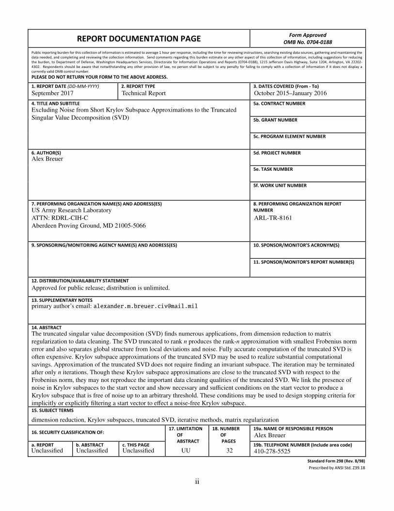
REPORT DOCUMENTATION PAGE Form Approved

OMB No. 0704‐0188

Public reporting burden for this collection of information is estimated to average 1 hour per response, including the time for reviewing instructions, searching existing data sources, gathering and maintaining the data needed, and completing and reviewing the collection information. Send comments regarding this burden estimate or any other aspect of this collection of information, including suggestions for reducing the burden, to Department of Defense, Washington Headquarters Services, Directorate for Information Operations and Reports (0704‐0188), 1215 Jefferson Davis Highway, Suite 1204, Arlington, VA 22202‐4302. Respondents should be aware that notwithstanding any other provision of law, no person shall be subject to any penalty for failing to comply with a collection of information if it does not display a currently valid OMB control number.

PLEASE DO NOT RETURN YOUR FORM TO THE ABOVE ADDRESS.

1. REPORT DATE (DD‐MM‐YYYY)

2. REPORT TYPE

3. DATES COVERED (From ‐ To)

4. TITLE AND SUBTITLE

5a. CONTRACT NUMBER

5b. GRANT NUMBER

5c. PROGRAM ELEMENT NUMBER

6. AUTHOR(S)

5d. PROJECT NUMBER

5e. TASK NUMBER

5f. WORK UNIT NUMBER

7. PERFORMING ORGANIZATION NAME(S) AND ADDRESS(ES)

8. PERFORMING ORGANIZATION REPORT NUMBER

9. SPONSORING/MONITORING AGENCY NAME(S) AND ADDRESS(ES)

10. SPONSOR/MONITOR’S ACRONYM(S)

11. SPONSOR/MONITOR'S REPORT NUMBER(S)

12. DISTRIBUTION/AVAILABILITY STATEMENT

13. SUPPLEMENTARY NOTES

14. ABSTRACT

15. SUBJECT TERMS

16. SECURITY CLASSIFICATION OF: 17. LIMITATION OF ABSTRACT

18. NUMBER OF PAGES

19a. NAME OF RESPONSIBLE PERSON

a. REPORT

b. ABSTRACT

c. THIS PAGE

19b. TELEPHONE NUMBER (Include area code)

Standard Form 298 (Rev. 8/98)

Prescribed by ANSI Std. Z39.18

September 2017 Technical Report

Excluding Noise from Short Krylov Subspace Approximations to the TruncatedSingular Value Decomposition (SVD)

Alex Breuer

ARL-TR-8161


October 2015–January 2016

US Army Research LaboratoryATTN: RDRL-CIH-CAberdeen Proving Ground, MD 21005-5066

primary author’s email: [email protected]

The truncated singular value decomposition (SVD) finds numerous applications, from dimension reduction to matrixregularization to data cleaning. The SVD truncated to rank n produces the rank-n approximation with smallest Frobenius normerror and also separates global structure from local deviations and noise. Fully accurate computation of the truncated SVD isoften expensive. Krylov subspace approximations of the truncated SVD may be used to realize substantial computationalsavings. Approximation of the truncated SVD does not require finding an invariant subspace. The iteration may be terminatedafter only n iterations. Though these Krylov subspace approximations are close to the truncated SVD with respect to theFrobenius norm, they may not reproduce the important data cleaning qualities of the truncated SVD. We link the presence ofnoise in Krylov subspaces to the start vector and show necessary and sufficient conditions on the start vector to produce aKrylov subspace that is free of noise up to an arbitrary threshold. These conditions may be used to design stopping criteria forimplicitly or explicitly filtering a start vector to effect a noise-free Krylov subspace.

dimension reduction, Krylov subspaces, truncated SVD, iterative methods, matrix regularization

32

Alex Breuer

410-278-5525Unclassified Unclassified Unclassified UU

ii


Contents

List of Figures iv

List of Tables v

Acknowledgments vi

1. Introduction 1

1.1 Summary of Contents 2

1.2 Dimension Reduction and the tSVD 3

1.3 Signal and Noise Spaces 4

1.4 Minimal Krylov Subspaces for Approximation of the tSVD 5

1.5 Approximate Eigenvectors and Eigenvalues from Krylov Subspaces 6

1.6 A Motivating Example 7

2. Corruption of Subspaces with Noise 9

2.1 Principal Angles for Quantifying Subspace Overlap 9

2.2 A Measure of Corruption: ρ-Free of Noise 10

3. Two Sufficient Conditions on z(0) for Kn(G, z(0)

)to Be ρ-Free of Noise 10

3.1 A Basic Sufficient Condition on z(0) for an Uncorrupted Subspace 10

3.2 A Sharper Sufficient Condition on z(0) 15

4. Conclusion 18

5. References 19

Distribution List 23

iii


List of Figures

Fig. 1 Spectrum of G as defined in Eq. 11................................................8

Fig. 2 Norms of G−1

and ‖x‖ ................................................................8

Fig. 3 Values of εmax, εcomputed, and ‖UTnoiseQ‖2 ........................................ 14

iv


List of Tables

Table 1 Computed values for max0≤x≤λp |q j(x)|, ‖q j(G)z(0)‖, probabilistic upperbounds on cosϑ

(ui, z j

), and computed maxui∈Unoise cosϑ

(ui, z j

)for the

Ritz vectors z j from K6

(G, z(0)

)................................................ 17

v


Acknowledgments

Dr Breuer would like to acknowledge the work of Dr Andrew Lumsdaine (PacificNorthwest National Laboratory) and Dr Geoffrey Sanders (Lawrence LivermoreNational Laboratory) who assisted in the preparation of this report.

vi


1. Introduction

Truncated singular value decompositions (tSVDs) are used for a variety of tasksin domains ranging from dimension reduction using principal component analysis(PCA),1 to eigenfaces2 in machine learning, to latent semantic indexing (LSI)3 in in-formation retrieval, matrix regularization,4,5 and sundry methods in signal process-ing.6,7 It is the core operation of data analysis techniques that use diagonal matrixfactorizations, such as PCA1,8 and proper orthogonal decomposition.9 In all cases,one is presented with M points a1, a2, . . . , am embedded in RN . These are assembledinto a matrix A ∈ RN×M; the goal is to find a reduced-dimension approximation Aof A, where A ∈ Rn×M, with n � N. With the tSVD, the data are projected intothe space spanned by a small subset of singular vectors; these are the n singularvectors that have the n largest singular values. In particular, the tSVD provides 2key advantages for dimension reduction applications:

• it approximates the data in a lower dimension; thereby reducing storage andprocessing costs while maintaining important features of the data, and

• it exhibits data cleaning properties by projecting into a space orthogonal todimensions along which variance is relatively small.

The latter of the above properties—data cleaning—is an important feature of tSVDmethods for dimension reduction and data approximation. Partitioning RN with thetSVD of A has been shown to separate global structure of columns of A from lo-cal deviations and noise.8,10 Global structure is represented by left singular vectorsof A with large singular values, while noise is represented by left singular vectorsof A with small singular values. Important dimension reduction methods that usethe tSVD exhibit better performance with reduced dimension data than with theoriginal, high-dimension data; for example, LSI produces reduced dimension ap-proximations that have better precision and recall than is witnessed with the samequeries on the original data.3,11

A chief drawback of tSVD methods is that they are computationally expensive. Thisdrawback has led several authors to develop approximations to the tSVD that arecomputationally cheaper. Several methods that substitute a Krylov subspace for atruncated singular vector space have been proposed,11–15 and they have shown greatpromise for reducing computational costs while only yielding small differences in

1


the sum-of-squared dimension reduction error of the tSVD. However, analyses ofthese Krylov subspace methods only have considered the sum-of-squares approx-imation error difference between the tSVD and a Krylov subspace approximation.The data cleaning properties are not considered.

It is somewhat well known that one cannot generate a sequence of Krylov subspacesthat are all orthogonal to the smallest extremal eigenvectors—ones with the smallesteigenvalues, no matter what one does to the start vector. Bounds in Golub et al.16

show this quantitatively; in fact, if one has a random start vector, then a Krylovsubspace used as a tSVD approximation may have a significant overlap with thenoise space (we quantitatively define the noise space in Section 1.3 and subspaceoverlap in Section 2.1) after a small number of iterations. Without filtering the startvector, the data cleaning properties of the Krylov subspace approximation methodsare poor. The presence of noise destroys the important data cleaning advantages oflow-rank data approximation.

1.1 Summary of Contents

Krylov subspace tSVD approximations11–15 will almost certainly not remove noiseas well as the tSVD when the start vector of the Krylov subspace is random. Evenwhen the start vector is not random, if the start vector is not orthogonal to all noisecontent, then noise will eventually be present in the Krylov subspace.

It is well known that the principal angles between a Krylov subspace and the noise-space vectors will shrink as one grows a Krylov subspace, no matter how closeto orthogonal the start vector is to the noise space. However, this relationship hasnot been well studied; there is no theory to predict how “noisy” a Krylov subspaceapproximation of the tSVD will be. Our main result bounds the noise content ofKrylov subspaces as dimension reduction projections. We present sufficient con-ditions that guarantee noise filtering of the Krylov subspace based on the noisecontent of the initial vector.

These sufficient conditions allow one to design a filtering procedure to producestart vectors that generate Krylov subspaces with bounded noise content. One mayuse Krylov subspace tSVD approximation methods, and enjoy the noise cleaningproperties of the tSVD while preserving the significant computational cost savingsof the Krylov subspace matrix approximation methods.11–15

2


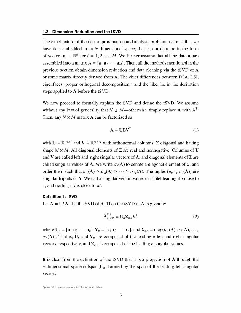
1.2 Dimension Reduction and the tSVD

The exact nature of the data approximation and analysis problem assumes that wehave data embedded in an N-dimensional space; that is, our data are in the formof vectors ai ∈ R

N for i = 1, 2, . . . ,M. We further assume that all the data ai areassembled into a matrix A = [a1 a2 · · · aM]. Then, all the methods mentioned in theprevious section obtain dimension reduction and data cleaning via the tSVD of Aor some matrix directly derived from A. The chief differences between PCA, LSI,eigenfaces, proper orthogonal decomposition,9 and the like, lie in the derivationsteps applied to A before the tSVD.

We now proceed to formally explain the SVD and define the tSVD. We assumewithout any loss of generality that N ≥ M—otherwise simply replace A with AT.Then, any N × M matrix A can be factorized as

A = UΣVT (1)

with U ∈ RN×M and V ∈ RM×M with orthonormal columns, Σ diagonal and havingshape M × M. All diagonal elements of Σ are real and nonnegative. Columns of Uand V are called left and right singular vectors of A, and diagonal elements of Σ arecalled singular values of A. We write σi(A) to denote a diagonal element of Σ, andorder them such that σ1(A) ≥ σ2(A) ≥ · · · ≥ σM(A). The tuples (ui, vi, σi(A)) aresingular triplets of A. We call a singular vector, value, or triplet leading if i close to1, and trailing if i is close to M.

Definition 1: tSVD

Let A = UΣVT be the SVD of A. Then the tSVD of A is given by

A(n)tSVD = UnΣn,nVT

n (2)

where Un = [u1 u2 · · · un], Vn = [v1 v2 · · · vn], and Σn,n = diag(σ1(A), σ2(A), . . . ,σn(A)). That is, Un and Vn are composed of the leading n left and right singularvectors, respectively, and Σn,n is composed of the leading n singular values.

It is clear from the definition of the tSVD that it is a projection of A through then-dimensional space colspan {Un} formed by the span of the leading left singularvectors.

3


Also, the n-dimensional tSVD is optimal with respect to the Frobenius norm, soA

(n)tSVD = arg minrank(A)=n ‖A − A‖F . The tSVD produces the reduction of A to n-

dimensions that is optimal in the least-squares sense aggregated over all ai.

1.3 Signal and Noise Spaces

We have noted that truncating the SVD also can de-noise the data. We define signaland noise spaces in terms of the SVD.

Definition 2: Signal and Noise Space

Suppose A is an arbitrary real matrix with SVD A = UΣVT. Let 0 < τ < 1 be anonnegative real number. Then the noise spaceUnoise of A is defined as

Unoise = span{up,up+1, . . . ,uM

}(3)

where p is the smallest natural number that satisfies√∑pi=1 σi(A)2∑Mi=1 σi(A)2

> τ. (4)

The signal spaceUsignal of A is then defined as the complement ofUnoise:

Usignal = U⊥noise. (5)

Remark 1. When the mean of the columns ai of A are zero centered and therefore∑Mi=1 ai = 0, the Gram matrix AAT satisfies AAT = sC, where s is some scalar and

C is the covariance matrix of the sample ai. In this case, a tSVD of A is equivalentto projecting out the N −n orthogonal dimensions along which variance is smallest.

Thus, the noise space of A is defined as the space in which less than τ of the Frobe-nius norm of A lies. It is clear that as τ→ 1, p approaches that index of the smallestnonzero singular value. This illustrates that the “noisiest” singular vectors are thosewith the smallest singular values.

When building a Krylov subspace for low-rank approximation, we want to guaran-tee that it is (nearly) orthogonal to these noisiest singular vectors for some τ that isclose to 1.

4


1.4 Minimal Krylov Subspaces for Approximation of the tSVD

Though the tSVD has these advantageous properties, it can be expensive to com-pute, especially if n is on the order of tens or more. A number of authors haveproposed Krylov subspaces as a surrogate for the leading singular vector space fordimension reduction tasks.11–15 Krylov subspaces are defined in terms of squarematrices. When A is not square, Krylov subspaces are typically defined in terms ofthe Gram matrices G = AAT or GT = ATA. These 2 Gram matrices transform thesingular value problem into an equivalent eigenvalue problem on G or GT; giventhe SVD A = UΣVT,

G = AAT = UΣ2UT (6)

andGT = ATA = VΣ2VT. (7)

Hereafter, when we write λi, it is implied that λi = λi(G) = λi(GT) = σi(A)2

Definition 3: Krylov Subspace

Suppose G = AAT with shape N × N and z(0) ∈ RN . Then the nth Krylov subspaceis given by

Kn

(G, z(0)

)= span

{z(0),Gz(0),G2z(0), . . . ,Gn−1z(0)

}. (8)

We call z(0) the start vector of the Krylov subspace. Approximation error of a sin-gular vector ui of A depends on the angle ϑ(z(0),ui) = cos−1

⟨z(0),ui

⟩/‖z(0)‖‖ui‖,

where 〈·, ·〉 is the inner product, and on the distribution of singular values of A. Thecloser z(0) is to ui—the larger cosϑ

(z(0),ui

)—the better the approximation of ui in

Kn

(G, z(0)

). When no beforehand information is available, z(0) is typically chosen

to be random.

Krylov subspace methods have been well proven as iterative SVD solvers.16,17 Oneprojects A into the intersection ofKn

(G, z(0)

)andKn

(GT,Gz(0)

), and each iteration

reduces approximation errors of extremal singular values. In fact, the tSVD is oftencomputed with a Krylov subspace solver. The difference is that to compute an n-dimensional tSVD, one will likely need to generate a Krylov subspace Kk

(G, z(0)

)with k � n, and/or repeatedly select a better start vector and generate a new Krylovsubspace. The tSVD approximation methods11–15 instead use k = n: a minimalKrylov subspace.

5


Definition 4: Minimal Krylov Subspace

The kth Krylov subspace Kk

(G, z(0)

)is said to be minimal for a reduction to n

dimensions if k = n.

Remark 2. In typical use of Krylov subspaces, one generates a subspace muchlarger than the solution space that is needed. The wanted solutions are then extractedfrom the Krylov subspace. For example, if one wants to compute n eigenvalues, onewill generate Kk

(G, z(0)

)with k > n, and often k � n. When all n eigenvectors are

invariant to tolerance, they are extracted from the Krylov subspace, and the problemis projected into the space spanned by those n computed eigenvectors.

1.5 Approximate Eigenvectors and Eigenvalues from Krylov Subspaces

An orthonormal basis z1, z2, . . . , zn of approximate eigenvectors of G may be ex-tracted from a Krylov subspace Kn

(G, z(0)

); alternately, these are approximate left

singular vectors of A. These vectors are also orthonormal and G-conjugate. We callan approximate eigenvector zi from a Krylov subspace a Ritz vector and the valueθi = zT

i Gzi a Ritz value. Any Ritz vector may be expressed as a linear combinationof eigenvectors of G.

A Ritz vector zi is not necessarily equal to the projection of an eigenvector QnQTn uiui

(where Qn is an orthonormal basis for Kn

(G, z(0)

)) through the Krylov subspace.

That is, we may—and very likely will—have zi , QnQTnui for all i. This is because

zi is defined as

zi = mindim(C)=i−1

arg maxx⊥C

xTGx‖x‖2

, (9)

while QnQTnui is given by

QnQTnui = arg min

x∈Kn(G,z(0))‖ui − x‖. (10)

In a minimal Krylov subspace, it is almost certain that there are many Ritz vectorsthat are not G-invariant; that is, the residual ‖Gvi − θivi‖ is greater than machineepsilon. Ritz vectors from Krylov subspaces are defined in terms of a polynomialq(x) whose roots are the Ritz values.18 Thus q(θi) = 0. Noise content of the Ritzvector depends on the ratio

∑Nj=p q(λ j)2

⟨z(0),u j

⟩2/∑N

j=1 q(λ j)2⟨z(0),u j

⟩2, where p

is from Definition 2. Whenever q(λ j)2⟨z(0)u j

⟩2is not tiny for j ≥ p, then the Ritz

vector may not be orthogonal to the noise space.

6


1.6 A Motivating Example

Constructing a linear classifier is a task that can motivate our discussion. A sim-ple way to construct a linear classifier is to solve Gx = µ1 − µ2, where G is thecovariance matrix and µ1 and µ2 are the means of the 2 classes. This problem isill-posed when G has small singular values (a nontrivial noise space), and we wanta classifier that is orthogonal to those dimensions along which variance is small.

The example is a matrix regularization problem. In matrix regularization prob-lems,19 one has a matrix G that has small singular values and one seeks a solu-tion that minimizes ‖Gx − b‖ but is also orthogonal to the singular vector spacecorresponding to the small singular vectors of G. The small singular values of Gmake minimization of ‖Gx − b‖ ill-posed, as small perturbations to b may resultin a large perturbation of x. One instead minimizes a regularized problem such as‖Gx − b‖ + η‖x‖, where η is a user-chosen regularization parameter picked to avoidsmall singular vectors of G. Using a tSVD can be as effective as directly minimizing‖Gx − b‖ + η‖x‖ for optimal η.4,5,20

If one substitutes a minimal Krylov subspace Kn

(G, z(0)

)with a random z(0) for

the truncated singular vector space, then the influence of small singular values isdifficult to control either directly, as with the tSVD, or indirectly, as in explicitminimization of ‖Gx − b‖ + η‖x‖. An x computed with an A

(n)from a minimal

Krylov subspace may have a large ‖x‖, which would have been avoided with evena small η.

Example 1. Let G be a 2, 000 × 2, 000 diagonal matrix defined as

G = diag(1, 1/2, 1/3, 1/4, . . . , 1/1999, 10−17). (11)

Since G is diagonal, its diagonal entries are its eigenvalues. Moreover, since allits eigenvalues are nonnegative, its spectral decomposition and SVD coincide. Thespectrum of G is shown in Fig. 1.

Set z(0) = 1/√

2000∑2000

i=1 ui. We have cosϑ(z(0),ui

)= 1/

√2000 for all eigenvec-

tors ui. We compute an orthonormal basis Qn for Kn

(G, z(0)

)and the G = QT

nGQfor 1 ≤ n ≤ 20. We generate a random b and solve the least squares problemx = arg miny ‖Tn,ny − b‖.

7


2000 1500 1000 500 0eigenvalue index

10-18

10-16

10-14

10-12

10-10

10-8

10-6

10-4

10-2

100

magnit

ude

Fig. 1 Spectrum of G as defined in Eq. 11

We compute the Frobenius norm of G−1

where G = QTnGQ for the Krylov subspace

solution or G = UnΣn,nUTn for the tSVD solution; the values are shown in Fig. 2.

Values of ‖x‖ are also shown for both the tSVD and minimal Krylov subspace x.Figures 1 and 2 show that substituting a minimal Krylov subspace for a truncatedsingular vector space for matrix regularization produces poorer regularization re-sults. The Frobenius norms of the G

−1from the minimal Krylov subspace are at

least 10 times larger than the tSVD G−1

, and the ‖x‖ are at least 100 times larger forthe minimal Krylov subspace.

0 5 10 15 20 25Krylov subspace dimension

10-2

10-1

100

101

102

103

104

jjG¡1jj F

SVD approximation

Kn (G;u(0) )

0 5 10 15 20 25Krylov subspace dimension

10-2

10-1

100

101

102

103

104

jjxjj

for min xjjGx¡bjj

SVD approximation

Kn (G;u(0) )

Fig. 2 Frobenius norms of G−1

, where G is G restricted to Kn

(G, z(0)

)or restricted to the

truncated singular vector space span {u1, . . . ,un} (left). Norms ‖x‖ where x is a solution to theleast squares problem ‖Gx − b‖ and where G = QT

n GQn where Qn is an orthonormal basis forKn

(G, z(0)

)or G = UnΣ

Tn,nUT

n (right). Large values indicate greater influence of small singularvectors in x and more sensitivity to small perturbations in b.

8


2. Corruption of Subspaces with Noise

When the basis vectors of the Krylov subspace are not orthogonal to the noise space,then the Krylov subspace has been “corrupted” by noise. The proceeding analysisrequires a measurement of how much a subspace is corrupted with noise. It is ev-ident that measurement of the corruption of a space S by noise is equivalent tomeasuring the norms of images of noise space basis vectors u j projected into S . Weuse the principal angles between spaces to formalize this concept.

2.1 Principal Angles for Quantifying Subspace Overlap

Much of the proceeding analysis considers the principal angles between spaces (seeZhu and Knyazev21[Definition 2.1 and Theorem 2.1]). We use these to quantify theoverlap between 2 subspaces ofRN . In the context of our analysis of minimal Krylovsubspaces for approximating the tSVD, we would like to have the overlap betweenKn

(G, z(0)

)andUnoise as small as possible.

Definition 5: Principal Angles

Let X and Y be matrices in RN with orthonormal columns. Then the principal anglesbetween colspan {X} and colspan {Y} are defined as

ϑ(X,Y) = [cos−1(σ1(XTY)) cos−1(σ2(XTY)) · · · ] = cos−1(σ(XTY)). (12)

When either X or Y has only one column, then there is only one principal angle.There is also a close relationship among the principal angles ϑ(X,Y), the Frobe-nius norm ‖XTY‖F , and the spectral norm ‖XTY‖2. The spectral norm is ‖XTY‖2 =√

cosϑ1 (X,Y)2 = σ1(XTY) and the Frobenius norm is ‖XTY‖F =

√∑ki=1 cosϑi (X,Y)2 =√∑k

i=1 σi(XTY)2 where XTY has k nonzero singular values.

Clearly, when colspan {X} ⊥ colspan {Y}, then ϑi(X,Y) = π/2 for all valid i, and‖XTY‖F = ‖XTY‖2 = 0. The closer all principal angles are to π/2, the smaller theoverlap between colspan {X} and colspan {Y}.

9


2.2 A Measure of Corruption: ρ-Free of Noise

Principal angles and the closely related matrix norms ‖ · ‖F and ‖ · ‖2 lead naturallyto a measure of the overlap between the noise space Unoise and some subspace S

with orthonormal basis W: ρ-free of noise.

Definition 6: ρ-Free of Noise

Let S ⊂ RN be some subspace, let W be an orthonormal basis for S, letUnoise ⊂ RN

be the noise space of G, and Unoise be an orthonormal basis for Unoise. Pick somenonnegative real ρ. Then S is ρ-free of noise if

cosϑ1 (Unoise,W) ≤ ρ. (13)

An equivalent condition to Eq. 13 is that ‖UTnoiseW‖2 ≤ ρ. Since ‖UT

noiseW‖2 ≤‖UT

noiseW‖F , ‖UTnoiseW‖F ≤ ρ also implies that S is ρ-free of noise.

3. Two Sufficient Conditions on z(0) for Kn

(G, z(0)

)to Be ρ-Free of Noise

We are now ready to present our main result. We develop 2 criteria that guaranteethat the nth Krylov subspace is ρ-free of noise.

3.1 A Basic Sufficient Condition on z(0) for an Uncorrupted Subspace

Our basic sufficient condition comes from Corollary 1, which depends on Lemma 1and Theorem 1. First, we use the Lanczos recurrence (see Saad,22 Section 3.2) tobound the cosine cosϑ

(qn+1,ui

)in Lemma 1, where qn+1 is a basis vector gener-

ated by the Lanczos algorithm.22 This result then leads to a recurrence relation thatbounds the image u(n)

i of the eigenvector ui projected intoKn

(G, z(0)

)in Theorem 1;

the sufficient condition in Corollary 1 on z(0) follows from that.

We begin with bounding the cosine cosϑ(qn+1,ui

).

Lemma 1

Let qn+1 be the n + 1th basis vector generated by the Lanczos algorithm actingon a Gram matrix G and z(0). Let Qn be an orthonormal basis for Kn

(G, z(0)

). Let

Tn,n = QTnGQn be the restriction of G to Kn

(G, z(0)

), and u(n)

i = QTnui. Note that

Tn,n is a tridiagonal matrix.22 Let βn+1 be the norm of the residual of the Lanczosalgorithm after the nth step. Order the singular values of a matrix A as σ1(A) ≥σ2(A) ≥ · · · ≥ σn(A), and the eigenvalues of G as λ1 ≥ λ2 ≥ · · · ≥ λN . Then

10


cosϑ(ui,qn+1

)obeys

cosϑ(ui,qn+1

)≤‖u(n)

i ‖σ1(Tn,n − Iλi)βn+1

.

Proof. Let Qn be the orthonormal basis generated for Kn

(G, z(0)

)by the Lanczos

algorithm after n steps. Then we have

GQn = QnTn,n + rneTn .

Write the inner product on RN as 〈·, ·〉. Left-multiplying both sides by uTi gives

uTi GQn = uT

i QnTn,n + uTi rneT

n

uTi GQn − uT

i QnTn,n = uTi rneT

n

andβn+1〈ui,qn+1〉e

Tn = uT

i GQn − uTi QnTn,n

as both qn+1βn+1 = rn. Then

βn+1|〈ui,qn+1〉| = βn+1‖〈ui,qn+1〉eTn‖ = ‖uT

i GQn − uTi QnTn,n‖

and

|〈ui,qn+1〉| =‖uT

i GQn − uTi QnTn,n‖

βn+1=‖λiu(n)T

i − u(n)Ti Tn,n‖

βn+1

as βn+1 ≥ 0. Noting that cosϑ(ui,qn+1

)= |〈ui,qn+1〉| when both vectors are unit-

length and‖u(n)T

i (Iλi − Tn,n)‖ ≤ ‖u(n)i ‖σ1(Tn,n − Iλi) (14)

completes the proof. �

Remark 3. Eq. 14 may also be bounded from below as

‖u(n)Ti (Iλi − Tn,n)‖ ≥ ‖u(n)

i ‖σn(Tn,n − Iλi).

One could use this result to obtain a different necessary condition for a noise-freeKrylov subspace.

11


We now use the result of Lemma 1 to bound ‖u(n)i ‖. This will result in a basic suffi-

cient condition.

Theorem 1

Let G, z(0), the λi, and Tn,n be defined as in Lemma 1. Let βk be any of the sub-and super-diagonal values of Tn,n, and let β ≤ βk for k = 1, 2, . . . , n. Let u(n)

i be theprojection of eigenvector ui into Kn

(G, z(0)

). Suppose that ‖u(0)

i ‖ ≤ ε and λi ≤ θ1,where θ1 is the principal eigenvalue of Tn,n. Then the norm of u(n)

i is bounded as

‖u(n)i ‖

2 ≤ ε2((λ1 − λi)2

β2 + 1)n−1

.

Proof. Let θ1 be the principal eigenvalue of Tn,n. We have 0 ≤ θ1 ≤ λ1—G is aGram matrix and 0 ≤ λN ≤ θ1—and it is assumed that λi ≤ θ1. Then we get

σ1(Tk,k − Iλi) ≤ λ1 − λi.

Applying Lemma 1 gives

cosϑ(ui,qn+1

)≤‖u(n)

i ‖(λ1 − λi)βn+1

≤‖u(n)

i ‖(λ1 − λi)β

.

Then we can express ‖u(n)i ‖ recursively, as

‖u(n)i ‖

2 = cosϑ(ui,qn

)2+ ‖u(n−1)

i ‖2.

So

‖u(n)i ‖

2 ≤‖u(n−1)

i ‖2(λ1 − λi)2

β2 + ‖u(n−1)i ‖2

≤ ‖u(n−1)i ‖2

((λ1 − λi)2

β2 + 1).

The closed form for this series is

‖u(n)‖2 ≤ ‖u(0)

i ‖2((λ1 − λi)2

β2 + 1)n−1

.

12


Since all noise eigenvectors have cosϑ(ui, z(0)

)≤ ε,

‖u(n)i ‖

2 ≤ ε2((λ1 − λi)2

β2 + 1)n−1

for any noise eigenvector ui. �

This result immediately leads to a sufficient condition on z(0) for Kn

(G, z(0)

)to be

ρ-free of noise.

Corollary 1

Let G and z(0) be given where eigenvalues of G are λ1 ≥ λ2 ≥ · · · ≥ λN , and letN − p be the dimension of the noise space Unoise. Suppose that ‖u(n)

i ‖ ≤ ε for anynoise eigenvector ui. Then Kn

(G, z(0)

)is ρ-free of noise if

ε2(N − p)((λ1 − λN)2

β2 + 1)n−1

≤ ρ2. (15)

This is due to an application of Theorem 1 to bound the quantity ‖u(n)N ‖, and noting

that ‖uTMQn‖ ≤ ‖UT

noiseQ‖2. This application of Theorem 1 is always possible, sinceλN is always less than or equal to any eigenvalue of Tn,n—the assumption that λN ≤

θ1 is always valid.

Remark 4. Corollary 1 uses a lower bound β on the Lanczos residuals β j. This valueis not known a priori, but it was conjectured g23 that no β j becomes negligible. Thecases for which β j does attain a small value is when the Krylov subspace is invariantor nearly so. We have observed that the median eigenvalue is often a reasonablelower bound on the β j from the Lanczos algorithm.

We now proceed with an example in which the median eigenvalue is a reasonablelower bound for β.

Example 2. We continue with the matrix G defined in Example 1. Set ρ = 0.001.SinceUnoise is defined by the trailing 100 eigenvectors, N − p = 100. We transformEq. 15 to a condition on ε:

ε ≤

√√√ρ2

(N − p)(

(λ1−λN )2

β2 + 1)n−1 . (16)

13


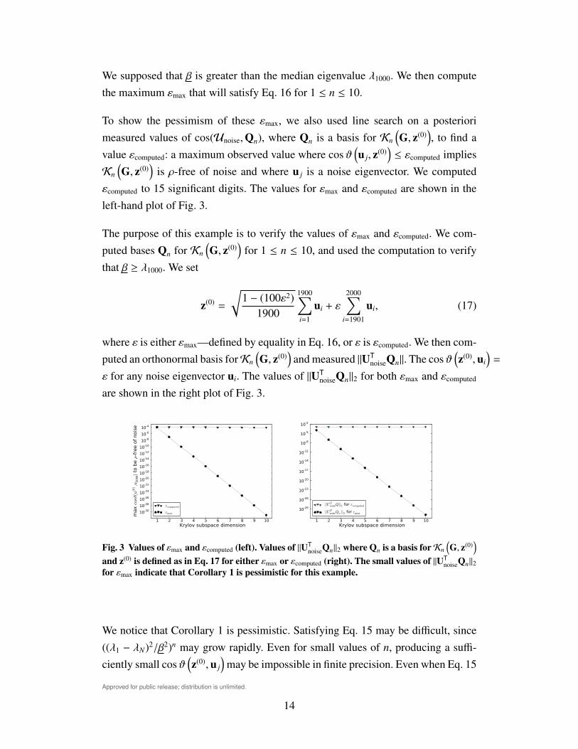
We supposed that β is greater than the median eigenvalue λ1000. We then computethe maximum εmax that will satisfy Eq. 16 for 1 ≤ n ≤ 10.

To show the pessimism of these εmax, we also used line search on a posteriorimeasured values of cos(Unoise,Qn), where Qn is a basis for Kn

(G, z(0)

), to find a

value εcomputed: a maximum observed value where cosϑ(u j, z(0)

)≤ εcomputed implies

Kn

(G, z(0)

)is ρ-free of noise and where u j is a noise eigenvector. We computed

εcomputed to 15 significant digits. The values for εmax and εcomputed are shown in theleft-hand plot of Fig. 3.

The purpose of this example is to verify the values of εmax and εcomputed. We com-puted bases Qn for Kn

(G, z(0)

)for 1 ≤ n ≤ 10, and used the computation to verify

that β ≥ λ1000. We set

z(0) =

√1 − (100ε2)

1900

1900∑i=1

ui + ε

2000∑i=1901

ui, (17)

where ε is either εmax—defined by equality in Eq. 16, or ε is εcomputed. We then com-puted an orthonormal basis forKn

(G, z(0)

)and measured ‖UT

noiseQn‖. The cosϑ(z(0),ui

)=

ε for any noise eigenvector ui. The values of ‖UTnoiseQn‖2 for both εmax and εcomputed

are shown in the right plot of Fig. 3.

1 2 3 4 5 6 7 8 9 10Krylov subspace dimension

10-30

10-28

10-26

10-24

10-22

10-20

10-18

10-16

10-14

10-12

10-10

10-8

10-6

10-4

max cos#(u(0);u2000)

to b

e ½

-fre

e o

f nois

e

"computed

"max

1 2 3 4 5 6 7 8 9 10Krylov subspace dimension

10-29

10-26

10-23

10-20

10-17

10-14

10-11

10-8

10-5

10-2

jjUTnoiseQjj2 for "computed

jjUTnoiseQn jj2 for "max

Fig. 3 Values of εmax and εcomputed (left). Values of ‖UTnoiseQn‖2 where Qn is a basis forKn

(G, z(0)

)and z(0) is defined as in Eq. 17 for either εmax or εcomputed (right). The small values of ‖UT

noiseQn‖2for εmax indicate that Corollary 1 is pessimistic for this example.

We notice that Corollary 1 is pessimistic. Satisfying Eq. 15 may be difficult, since((λ1 − λN)2/β2)n may grow rapidly. Even for small values of n, producing a suffi-ciently small cosϑ

(z(0),u j

)may be impossible in finite precision. Even when Eq. 15

14


is not satisfied, it may be the case that the Krylov subspace is ρ-free of noise. There-fore, we present a tighter a posteriori sufficient condition that uses information fromthe Krylov subspace.

3.2 A Sharper Sufficient Condition on z(0)

We notice that the basic sufficient condition is pessimistic, and not practical forn greater than 10 or so. Our second sufficient condition gives us extra sharpnessto extend a sufficient condition for larger n. Lemma 2, about the polynomial thatdefines Ritz vectors, directly gives another sufficient condition, which we illustratein Example 3. A nice feature of the condition that comes from Lemma 2 is that thequantities can be computed from byproducts of the Lanczos algorithm, as is notedin Remark 5.

Lemma 2

Let the positive semidefinite matrix G and vector z(0) define the Krylov subspaceKn

(G, z(0)

), and let θ1 ≥ θ2 ≥ · · · ≥ θn be the Ritz values of the restriction of G to

Kn

(G, z(0)

), with unit-length Ritz vectors z1, z2, . . . , zn. Define the polynomial q j(x)

as

q j(x) =

n∏t = 1k , j

(x − θk)

and set ci =⟨z(0),ui

⟩, where 〈·, ·〉 is the inner product on RN . Suppose p ≤ i ≤ N.

Then the magnitude of the cosine cosϑ(ui, z j

)is bounded as

cosϑ(ui, z j

)≤ max

0≤x≤λp

|q j(x)ci|

‖q j(G)z(0)‖.

Proof. The polynomial

q j(x) =

n∏t = 1k , j

(x − θk)

15


gives the jth Ritz vector of Kn

(G, z(0)

);18

(z j = q j(G)z(0)/‖q j(G)z(0)‖

). Therefore,

cosϑ(ui, z j

)=|q j(λi)ci|

‖q j(G)z(0)‖.

Since i ≤ p and G is positive semidefinite, 0 ≤ λi ≤ λp and |q j(λi)| ≤ max0≤x≤λp |q(x)|.Then

cosϑ(ui, z j

)= max

0≤x≤λp

|q j(x)ci|

‖q j(G)z(0)‖,

which completes the proof. �

Remark 5. The polynomial q j(x) and the norm ‖q j(G)z(0)‖ can be computed a pos-teriori inexpensively as a by-product of a standard Krylov subspace algorithm, suchas the Lanczos algorithm. However, ci is typically unknown, but can be boundedif z(0) has known properties. For example, if z(0) is a random vector, then |ci| maybe probabilistically bounded with enough tightness as to result in tight bounds forcosϑ (ui, z). For our example case, where eigenvectors are all standard basis vectors(in Dettman,24 p. 111) and 〈ui, x〉 = xi for xi is the ith entry of x, this is straightfor-ward.

Example 3. Let G be defined as in Example 1. Set z(0) to be a random vector withentries drawn from the normal distribution N(0, 1). We compute K6

(G, z(0)

)and

compute the Ritz values and q j(x) for 1 ≤ j ≤ 6. Each q j(x) is a quintic polynomial;their derivatives give their maxima between Ritz values θi, are quartic, and can besolved analytically. We computed θ6 > λN and max0≤x≤λp |q j(x)| ≤ max0≤x≤θ6 |q j(x)|,so it is sufficient to consider maxima of |q j(x)| for 0 ≤ x ≤ θ6. For all q j(x), |q j(0)| =max0≤x≤λp |q j(x)|. We now proceed to bound ci.

Since z(0) is random, zero-centered, and normally distributed, we may place anupper bound on cosϑ

(z(0),u j

)by noticing that the standard basis vectors24 e j =

[0 0 · · · 0 1 0 · · · 0] are eigenvectors of G. Then u j = e j and

c j =

⟨u j, z(0)

⟩‖z(0)‖

=z(0)

j

‖z(0)‖

where z(0)j is the jth entry of z(0). As entries of z(0) are drawn from N(0, 1), the

squared norm of z(0) follows a Chi-squared distribution with N − 1 degrees of free-dom. Write CN(0,1)(a) as the critical value N(0, 1) and probability a, and Cχ2(a,N)

16


is the critical value for χ2N and probability a. Then, with probability 1 − 2a,

CN(0,1)(1 − a)√Cχ2(1 − a,N − 1)

≤ ci ≤CN(0,1)(a)√

Cχ2(1 − a,N − 1).

Due to the symmetry of N(0, 1), this is equivalent to

|ci| ≤CN(0,1)(a)√

Cχ2(a,N − 1).

For a = 0.99 and N = 2000, we have CN(0,1)(a) ≈ 2.33 and Cχ2(1 − a,N − 1) ≈1854.86. Then |ci| ≤ 0.0542 with probability at least 0.99.

We combine this upper bound on |ci| with the computed maxima of ‖q j(x)‖ over[0, λp] and the values of |q j(G)z(0)| to get upper bounds on cosϑ

(ui, z j

). The re-

sults are shown in Table 1, and we compare these with the computed values formaxui∈Unoise cosϑ

(ui, z j

). The upper bounds on cosϑ

(ui, z j

)are tighter than those

produced from Corollary 1. Also, it is clear from Table 1 that the space span {z2, z1}

is ρ-free of noise for all ρ ≥ 0.0007.

Table 1 Computed values for max0≤x≤λp |q j(x)|, ‖q j(G)z(0)‖, probabilistic upper bounds oncosϑ

(ui, z j

), and computed maxui∈Unoise cosϑ

(ui, z j

)for the Ritz vectors z j from K6

(G, z(0)

).

Small values of ‖q j(G)z(0)‖ contribute substantially to large upper bounds on cosϑ(u j, zi

).

Quantity z6 z5 z4 z3 z2 z1

max0≤x≤θ6

|q j(x)| 8.05×10−4 3.55×10−5 8.32×10−6 4.40×10−6 2.56×10−6 1.28×10−6

‖q j(G)z(0)‖ 7.4×10−4 7.8×10−5 4.19×10−5 4.68×10−5 2.1×10−4 5.56×10−3

probabilistic max 5.87×10−2 2.46×10−2 1.07×10−2 5.09×10−3 6.69×10−4 1.25×10−5

cosϑ(u j, zi

)ci boundedwith a = 0.99computed max 4.02×10−2 1.16×10−2 5×10−3 2.37×10−3 3.11×10−4 5.78×10−6

cosϑ(u j, zi

)

The bounds in Lemma 2 indicate that noise may be due to either a large value ofmax0≤x≤λp |q j(x)ci| or due to a relatively small value of ‖q j(G)z(0)‖.

17


4. Conclusion

We have presented sufficient conditions for a Krylov subspace approximation of thetSVD to be ρ-free of noise. Generally speaking, one can see that minimal Krylovsubspace substitutions for the tSVD are doomed to be noisy if n is large enough,even if the start vector is orthogonal to the noise space up to machine precision.However, for moderate n, one can use the sufficient conditions to design a filter toproduce a start vector z(0) that has a small enough cosϑ

(ui, z(0)

)for noise space

ui so that Kn

(G, z(0)

)is ρ-free of noise. We are then motivated to find methods to

compute good start vectors for minimal Krylov subspaces.

When considering methods to prepare start vectors that satisfy the sufficient con-ditions presented here, we recall the overarching purpose for minimal Krylov sub-space approximations to the tSVD: dramatically smaller compute times. Start vec-tor generation methods that have smaller computational costs are preferable. Startvectors may be implicitly filtered with either Implicitly-Restart Lanczos25 or Thick-Restart Lanczos26 when n is small, and Lemma 2 gives a criterion for which Ritzvectors to discard. When n is large, the asymptotic cost of computing Ritz vectors—O(n2N)—may become prohibitive. Implicit start vector filtering may also be less at-tractive when matrix-vector products scale better than dot products or matrix norms,as is the case for some classes of distributed matrices. Then filtering methods, suchas Chebyshev polynomials or approximation of sigmoidal functions27 may be lessexpensive. Since G is a positive semi-definite matrix, simple power iteration on ablock vector as in Halko et al.28 may also be an effective method for preparing astart vector that satisfies our sufficient conditions.

18


5. References

1. Jolliffe I. Principal component analysis. New York (NY): Springer-Verlag;2002.

2. Turk M, Pentland A. Eigenfaces for recognition. Journal of Cognitive Neuro-science. 1991;3(1):71–86.

3. Deerwester S, Dumais S, Furnas G, Landauer T, Harshman R. Indexing bylatent semantic analysis. Journal of the American Society for Information Sci-ence. 1990;41(6):391–407.

4. Hansen PC. Truncated singular value decomposition solutions to discrete ill-posed problems with ill-determined numerical rank. SIAM Journal on Scien-tific and Statistical Computing. 1990;11(3):503–518.

5. Hansen PC, Sekii T, Shibahashi H. The modified truncated SVD method forregularization in general form. SIAM Journal on Scientific and Statistical Com-puting. 1992;13(5):1142–1150.

6. Schelter B, Winterhalder M, Timmer J. Handbook of time series analysis: re-cent theoretical developments and applications. Weinheim (Germany): Wiley-VCH Verlag GmbH & Co. KGaA; 2006.

7. Hyvärinen A, Hurri J, Hoyer P. Natural image statistics: a probabilistic ap-proach to early computational vision. New York (NY): Springer-Verlag; 2009.(Computational Imaging and Vision).

8. Skillicorn D. Understanding complex datasets: data mining with matrix de-compositions. New York (NY): Chapman & Hall/CRC; 2007.

9. Liang Y, Lee H, Lim S, Lin W, Lee K, Wu C. Proper orthogonal decompo-sition and its applications — part I: theory. Journal of Sound and Vibration.2002;252(3):527–544.

10. Fukunaga K. Introduction to statistical pattern recognition. San Diego (CA):Academic Press; 1990.

11. Blom K, Ruhe A. A Krylov subspace method for information retrieval. SIAMJournal on Matrix Analysis and Applications. 2004;26(2):566–582.

19


12. Simon H, Zha H. Low-rank matrix approximation using the Lanczos bidiag-onalization process with applications. SIAM Journal on Scientific Computing.2000;21(6):2257–2274.

13. Chen J, Saad Y. Lanczos vectors versus singular vectors for effective di-mension reduction. IEEE Transactions on Knowledge and Data Engineering.2009;21(8):1091–1103.

14. Elden L. Matrix methods in data mining and pattern recognition. Philadelphia(PA): Society for Industrial and Applied Mathematics; 2007.

15. Ren CX, Dai DQ. Bilinear Lanczos components for fast dimensionality reduc-tion and feature extraction. Pattern Recognition. 2010;43(11):3742–3752.

16. Golub G, Luk F, Overton M. A block Lanczos method for computing the sin-gular values and corresponding singular vectors of a matrix. ACM Transactionson Mathematical Software (TOMS). 1981;7(2):149–169.

17. Bai Z. Templates for the solution of algebraic eigenvalue problems. Philadel-phia (PA): Society for Industrial Mathematics; 2000.

18. Saad Y. On the rates of convergence of the Lanczos and the block-Lanczosmethods. SIAM Journal on Numerical Analysis. 1980;17(5):687–706.

19. Golub G, Van Loan C. Matrix computations. Baltimore (MD): Johns HopkinsUniversity Press; 2013.

20. Hansen PC. The truncated SVD as a method for regularization. BIT NumericalMathematics. 1987;27(4):534–553.

21. Zhu P, Knyazev A. Angles between subspaces and their tangents. Journal ofNumerical Mathematics. 2013;21(4):325–340.

22. Saad Y. Numerical methods for large eigenvalue problems. Manchester (UK):Manchester University Press; 1992.

23. Simon H. Analysis of the symmetric Lanczos algorithm with reorthogonaliza-tion methods. Linear Algebra and Its Applications. 1984;61:101–131.

24. Dettman J. Introduction to linear algebra and differential equations. New York(NY): Dover; 1986.

20


25. Calvetti D, Reichel L, Sorensen D. An implicitly restarted Lanczos method forlarge symmetric eigenvalue problems. Electronic Transactions on NumericalAnalysis. 1994;2(1):1–21.

26. Wu K, Simon H. Thick-restart Lanczos method for large symmetriceigenvalue problems. SIAM Journal on Matrix Analysis and Applications.2000;22(2):602–616.

27. Kokiopoulou E, Saad Y. Polynomial filtering in latent semantic indexing forinformation retrieval. Proceedings of the 27th Annual International ACM SI-GIR Conference on Research and Development in Information Retrieval; 2004July 25–29; Sheffield, (UK). New York, (NY): ACM; 2004. p. 104–111.

28. Halko N, Martinsson P, Tropp J. Finding structure with randomness: proba-bilistic algorithms for constructing approximate matrix decompositions. SIAMReview. 2011;53(2):217–288.

21


Intentionally left blank.

22


1(PDF)

DEFENSE TECHNICALINFORMATION CTRDTIC OCA

2(PDF)

DIRECTORUS ARMY RESEARCH LABRDRL CIO LIMAL HRA MAIL & RECORDS MGMT

1(PDF)

GOVT PRINTG OFCA MALHORTA

2(PDF)

DIR USARLRDRL CIH C

E CHINA BREUER

23


Intentionally left blank.

24

Documents

Excluding Noise from Short Krylov Subspace … norm, they may not reproduce the important data cleaning qualities of the truncated SVD. We link the presence of noise in Krylov subspaces