EXCHANGE RATE REGIMES, CAPITAL FLOWS

AND

CRISIS PREVENTION

By

Sebastian Edwards

University of California, Los Angeles

And

National Bureau of Economic Research

October, 2000

Revised: September 2001

* This is a revised version of a paper prepared for the National Bureau of Economic

Research Conference on “Economic and Financial Crises in Emerging Market

Economies,” held in Woodstock, October 19-21, 2000. I have benefited from

conversations with Ed Leamer. I thank Marty Feldstein for comments.

1

I. Introduction

The emerging markets financial crises of the 1990s had remarkable similarities.1

Attracted by high domestic interest rates, a sense of stability stemming from rigid

exchange rates, and what at the time appeared to be rosy prospects, large volumes of

foreign portfolio funds moved into Latin America, East Asia and Russia. This helped

propell stock market booms and helped finance large current account deficits. At some

point, and for a number of reasons, these funds slowed down and/or were reversed. This

change in conditions required significant corrections in macroeconomics policies.

Invariably, however, adjustment was delayed or was insufficient, increasing the level of

uncertainty and the degree of country risk. As a result, massive volumes of capital left

the country in question, international reserves dropped to dangerously low levels and real

exchange rates became acutely overvalued. Eventually the pegged nominal exchange rate

had to be abandoned, and the country was forced to float its currency. In some cases --

Brazil and Russia are the clearest examples --, a severe fiscal imbalance made the

situation even worse.

Recent currency crises have tended to be deeper than in the past, resulting in steep

costs to the population of the counties involved. In a world with high capital mobility,

even small adjustments in international portfolio allocations to the emerging economies

result in very large swings in capital flows. Sudden reductions in these flows, in turn,

amplify exchange rate and/or interest rate adjustments and generate overshooting, further

bruising credibility and unleashing a vicious circle. Two main policy issues have been

emphasized in recent discussions on crises prevention: First, an increasing number of

authors have argued that in order to prevent crises, there is a need to introduce major

changes to exchange rate practices in emerging economies. According to this view,

emerging economies should adopt “credible” exchange rate regimes. A “credible”

regime would reduce the probability of rumors-based reversals in capital flows, including

what some authors have called have called “sudden stops.” These authors have pointed

out that the emerging economies should follow a “two-corners” approach to exchange

rate policy: they should either adopt a freely floating regime, or a super-fixed exchange

1 I am referring to the crises in Mexico (1997), East Asia (1997), Russia (1998) and Brazil (1999).

2

rate system.2 Second, a number of analysts have argued that the imposition of capital

controls – and in particular controls on capital inflows -- provides an effective way for

reducing the probability of a currency crisis.

The purpose of this paper is to analyze, within the context of the implementation

of a new “financial architecture,” the relationship between exchange rate regimes, capital

flows and currency crises in emerging economies. The paper draws on lessons learned

during the 1990s, and deals with some of the most important policy controversies that

emerged after the Mexican, East Asian, Russian and Brazilian crises. I also evaluate some

recent proposals for reforming the international financial architecture that have

emphasized exchange rate regimes and capital mobility. The rest of the paper is

organized as follows: In section II I review the way in which economists’ thinking about

exchange rates in emerging markets has changed in the last decade and a half. More

specifically, in this section I deal with four interrelated issues: (1) The role of nominal

exchange rates as nominal anchors. (2) The costs of real exchange rate overvaluation. (3)

Strategies for exiting a pegged exchange rate. And (4), the “death” of middle-of the-road

exchange rate regimes as policy options. In Section III I deal with capital controls as a

crisis-prevention device. In this section Chile’s experience with market-based controls

on capital inflows is discussed in some detail. Section IV focuses on the currently

fashionable view that suggests that emerging countries should freely float or adopt a

super-fixed exchange rate regime (i.e. currency board or dollarization). In doing this I

analyze whether emerging markets can adopt a truly freely floating exchange rate system,

or whether, as argued by some analysts, a true floating system in not feasible in less

advanced nations. The experiences of Panama and Argentina with super-fixity, and of

Mexico with a floating rate are discussed in some detail. Finally, section V contains

some concluding remarks.

II. Exchange Rate Lessons from the 1990s Currency Crises

The currency crises of the 1990s have led economists to rethink their views on

exchange rate policies in emerging countries. Specifically, these crises have led many

economists to question the merits of pegged-but-adjustable exchange rates, both in the

short run – that is, during a stabilization program – as well as in the longer run. Indeed,

2 Summers (2000).

3

the increasingly dominant view among experts is that, in order to prevent the recurrence

of financial and currency crises, most emerging countries should adopt either freely

floating or super-fixed exchange rate regimes. In this section I discuss the way in which

policy thinking on exchange rates in emerging countries has evolved in the last decade

and a half or so.

II.1 Nominal Anchors and Exchange Rates

In the late 1980s and early 1990s, and after a period of relative disfavor, rigid

nominal exchange rates made a comeback in policy and academic circles. Based on

time-consistency and political economy arguments, a number of authors argued that

fixed, or predetermined, nominal exchange rates provided an effective device for guiding

a disinflation program, and for maintaining macroeconomic stability. According to this

view, an exchange rate anchor was particularly effective in countries with high inflation –

say, high two digits levels – that had already tackled (most of) their fiscal imbalances.

By imposing a “ceiling” on tradable prices, and by guiding inflationary expectations, it

was said, an exchange rate nominal anchor would rapidly generate a convergence

between the country’s and the international rates of inflation. This view was particularly

popular in Latin America, and was behind major stabilization efforts in Argentina, Chile

and Mexico, among others. According to this perspective, a prerequisite for a successful

exchange rate-based stabilization program was that the country in question had put its

public finances in order, before the program was implemented in full. This, indeed, had

been the case in Chile in 1978-79 and Mexico during the late 1980s and early 1990s,

when the so-called Pacto de Solidaridad exchange rate-based stabilization program was

implemented (see Edwards and Edwards 1991, Aspe 1993).

However, a recurrent problem with exchange rate-based stabilization programs –

and one that was not fully anticipated by its supporters —was that inflation tended to

have a considerable degree of inertia. That is, in most episodes domestic prices and

wages continued to increase even after the nominal exchange rate had been fixed. In

Edwards (1998c) I used data from the Chilean (1977-1982) and Mexican (1988-1994)

exchange rate-based stabilizations, to analyze whether the degree inflationary persistence

declined once the nominal exchange rate anchor program was implemented. My results

suggest that, in both cases, the degree of persistence did not change significantly, and

4

remained very high. I attributed these results to two factors: a rather low degree of

credibility of the programs, and, particularly in the case of Chile, the effects of a

backward looking wage-rate indexation mechanism.

If inflation is indeed characterized by a high degree of inertia, a fixed – or

predetermined -- nominal exchange rate will result in a real exchange rate appreciation,

and consequently in a decline in exports’ competitiveness. Dornbusch (1997, p. 131)

forcefully discussed the dangers of exchange rate anchors in his analysis of the Mexican

crisis:

“Exchange rate-based stabilization goes through three phases: The first

one is very useful…[E]xchange rate stabilization helps bring under way a

stabilization…In the second phase increasing real appreciation becomes

apparent, it is increasingly recognized, but it is inconvenient to do

something…Finally, in the third phase, it is too late to do something. Real

appreciation has come to a point where a major devaluation is necessary.

But the politics will not allow that. Some more time is spent in denial, and

then – sometime – enough bad news pile up to cause the crash.”

An additional complication is that under pegged exchange rates, negative external

shock tend to generate a costly adjustment process. Indeed, in a country with fixed

exchange rates the optimal reaction to a negative shock – a worsening of the terms of

trade or a decline in capital inflows, for example — is tightening monetary and fiscal

policies, until external balance is re-established. A direct consequence of this is that as a

result of these negative shocks, economic activity will decline, and the rate of

unemployment will tend to increase sharply. If the country is already suffering from a

real exchange rate overvaluation, this kind of adjustment becomes politically difficult.

More often than not countries that face this situation will tend to postpone the required

macroeconomics tightening, increasing the degree of vulnerability of the economy.

Following this kind of reasoning, and after reviewing the fundamental aspects of the

Mexican crisis, Sachs, Tornell and Velasco (1995 p. 71) argue that it is “hard to find

cases where governments have let the [adjustment process under fixed exchange rate] run

5

its course.” According to them, countries’ political inability (or unwillingness) to live

according to the rules of a fixed exchange rate regime, reduces its degree of credibility.

In the mid-1990s, even as professional economists in academia and the

multilateral institutions questioned the effectiveness of pegged-but-adjustable rates,

policy makers in the emerging economies continued to favor that type of policies. In

spite of Mexico’s painful experience with a rigid exchange rate regime in the first half of

the 1990s, the five East Asian nations that eventually run into a crisis in 1997 had a

rigid—de facto, pegged or quasi pegged—exchange rate system with respect to the US

dollar. Whereas this system worked relatively well while the US dollar was relatively

weak in international currency markets, things turned to the worse when, starting in mid

1996, the dollar began to strengthen relative to the Japanese yen. Naturally, as the dollar

appreciated relative to the yen, so did those currencies pegged to it. Ito (2000) has

described the role of pegged exchange rates in the East Asian crisis in the following way:

“[T]he exchange rate regime was de facto dollar pegged. In the period of yen

appreciation, Asian exporters enjoy high growth contributing to an overall high,

economic growth, while in the period of yen depreciation, Asian economies’

performance becomes less impressive…Moreover, the dollar peg with high

interest rates invited in short-term portfolio investment. Investors and borrowers

mistook the stability of the exchange rate for the absence of exchange rate risk”

(page 280).

In Russia and Brazil the reliance on rigid exchange rates was even more risky than in

Mexico and in the East Asian nations. This was because in both Russia and Brazil the

public sector accounts were clearly out of control. In Russia, for example, the nominal

deficit averaged 7.4% of GDP duringin the three years preceding the crisis. Worse yet,

the lack of accountability during the privatization process, and the perception of massive

corruption had made international investors particularly skittish. In Brazil, the real plan,

launched in 1994, relied on a very slowly moving pre-announced parity with respect tpo

the U.S. dollar. In spite of repeated efforts, the authorities were unable to reign in a very

6

large fiscal imbalance. By late 1998 the nation’s consolidated nominal fiscal deficit

exceeded the astonishing level of 8% of GDP.

II.2 Real Exchange Rate Overvaluation: How Dangerous? How to Measure it?

The currency crises of the 1990s underscored the need of avoiding overvalued

real exchange rates—that is, real exchange rates that are incompatible with maintaining

sustainable external accounts. In the spring 1994 meetings of the Brookings Institution

Economics Panel, Rudi Dornbusch argued that the Mexican peso was overvalued by at

least 30 percent, and that the authorities should rapidly find a way to solve the problem.

In that same meeting, Stanley Fischer, soon to become the IMF’s First Deputy Managing

Director, expressed his concerns regarding the external sustainability of the Mexican

experiment. Internal U.S. government communications released to the U.S. Senate

Banking Committee during 1995 also reflects a mounting concern among some U.S.

officials. Several staff members of the Federal Reserve Bank of New York, for example,

argued that a devaluation of the peso could not be ruled out. For example, according to

documents released by the U.S. Senate, on October 27th, 1994 an unidentified Treasury

Staff commented to Secretary Lloyd Bensten that:

“[rigid] exchange rate policy under the new Pacto [the tripartite incomes policy

agreement between government, unions and the private sector]could inhibit a

sustainable external position. (D’amato 1995, p. 308).

The overvaluation of the Mexican peso in the process leading to the 1994

currency crisis has been documented by a number of post-crisis studies. According to

Sachs, Tornell and Velasco (1996), for example, during the 1990-94 period the Mexican

peso was overvalued, on average, by almost 29 percent (see their table 9). An ex-post

analysis by Ades and Kaune (1997), using a detailed empirical model that decomposed

fundamentals’ changes in permanent and temporary, indicates that by the fourth quarter

of 1994 the Mexican peso was overvalued by 16 percent. According to Goldman_Sachs,

in late 1998 the Brazilian real was overvalued by approximately 14%. And although the

investment houses did not venture to estimate the degree of misalignment of the Russian

7

ruble, during the first half of 1997 there was generalized agreement that it had become

severely overvalued.

The East Asian nations did not escape the real exchange rate overvaluation

syndrome. Sachs, Tornell and Velasco (1996), for instance, have argued that by late

1994 the real exchange rate picture in the East Asian countries was mixed and looked as

follows: While the Philippines and Korea were experiencing overvaluation, Malaysia

and Indonesia had undervalued real exchange rates, and the Thai Baht appeared to be in

equilibrium. Chinn (1998) used a standard monetary model to estimate the

appropriateness of nominal exchange rates in East Asia before the crisis. According to

his results, in the first quarter of 1997 Indonesia, Malaysia and Thailand had overvalued

exchange rates, while Korea and the Philippines were facing undervaluation.

After the Mexican and East Asian crises, analysts in academia, the multilaterals

and the private sector have redoubled their efforts to understand real exchange rate

behavior in emerging economies. Generally speaking, the RER is said to be “misaligned”

if its actual value exhibits a (sustained) departure from its long run equilibrium. The

latter, in turn, is defined as the real exchange rate that, for given values of

“fundamentals,” is compatible with the simultaneous achievement of internal and

external equilibrium.3 Most recent efforts to assess misalignment have tried to go beyond

simple versions of purchasing power parity (PPP), and to incorporate explicitly the

behavior of variables such as terms of trade, real interest rates and productivity growth.

Accordingly to a recently published World Bank book (Hinkle and Montiel 1999), one of

the most common methods for assessing real exchange rates is based on single equation,

time series econometric estimates. The empirical implementation of this approach is

based on the following steps:

• A group of variables that, according to theory, affect the real exchange rate is

identified. These variables are called the real exchange rate “fundamentals,” and

usually include the country’s terms of trade, its degree of openness, productivity

differentials, government expenditure, direct foreign investment and international

interest rates.

3 For theoretical discussions on real exchange rates, see Frenkel and Razin (1987) and Edwards (1989).

8

• Time series techniques are used to estimate a real exchange rate equation. The

regressors are the “fundamentals” listed above. In most cases an error correction

model is used to estimate this equation.

• The “fundamentals” are decomposed into a “permanent” and a “temporary”

component. This is usually done by using a well-accepted statistical technique,

such as the Hodrick-Prescott decomposition.

• The permanent components of the fundamentals are inserted into the estimated

real exchange rate equation. The resulting “fitted” time series is interpreted as the

path through time of the estimated equilibrium real exchange rate.

• Finally, the estimated equilibrium real exchange rate is compared to the actual

RER. Deviations between these two rates are interpreted as misalignment. If the

actual real exchange rate is stronger that the estimated equilibrium, the country in

question is considered to face a real exchange rate overvaluation.

In the late 1990s Goldman-Sachs (1997) implemented a real exchange rate model

(largely) based on this methodology. The first version of this model, released in October

of 1996 – almost eight months before the eruption of the East Asian crisis --, indicated

that the real exchange rate was overvalued in Indonesia, the Philippines and Thailand.

Subsequent releases of the model incorporated additional countries, and suggested that

the Korean won and the Malaysian ringgit were also (slightly) overvalued. In mid 1997,

Goldman-Sachs introduced a new refined version of its model; according to these new

estimates, in June of 1997 the currencies of Indonesia, Korea, Malaysia, the Philippines,

and Thailand were overvalued, as were the currencies of Hong Kong and Singapore. In

contrast, these calculations suggested that the Taiwanese dollar was undervalued by

approximately 7 percent. Although according to G-S, in June 1997 the degree of

overvaluation was rather modest in all five East Asian-crisis countries, its estimates

suggested that overvaluation had been persistent for a number of years: in Indonesia the

real exchange rate had been overvalued since 1993, in Korea in 1988, in Malaysia in

1993, in the Philippines in 1992, and in Thailand since 1990 (See Edwards and Savastano

1999 for a review of other applications of this model for assessing real exchange rate

overvaluation).

9

More recently J.P. Morgan (2000) unveiled its own real exchange rate model. In

an effort to better capture the dynamic behavior of real exchange rates this model went

beyond the “fundamentals,” and explicitly incorporated the role of monetary variables in

the short run. In spite of this improvement, this model retained many of the features of

the single equation RER models summarized above, and analyzed in greater detail in

Edwards and Savastano (1999).

Although the methodology described above – and increasingly used by the

multilateral institutions and investment banks -- represents a major improvement over

simple Purchasing Power Parity-based calculations, it is still subject to some limitations.

The most important one is that, as is the case in all residuals-based models, it assumes

that the real exchange rate is, on average, in equilibrium during the period under study.

This, of course, needs not be the case. Second, this approach ignores the role of debt

accumulation, and of current account dynamics. Third, the more simple applications of

this model ignore the major jumps in the real exchange rate, following a nominal

devaluation. This, in turn, will tend to badly bias the results, and will tend to generate

misleading predictions. A fourth shortcoming of these models is that they do not specify

a direct relationship between the estimated equilibrium real exchnage rate and measures

of internal equilibrium, including the level of unemployment, or the relation between

actual and potential growth. And fifth, many times this type of econometric-based

anlaysis generate results that are counterintuitive and, more seriously perhaps, tend to

contradict the conclusions obtained from more detailed country-specific studies (see

Edwards and Svastano 1999 for a detailed discussion).

An alternative approach to evaluate the appropriateness of the real exchnage rate

at a particular moment in time, consists of calculating the “sustainable” current account

deficit, as a prior step to calculating the equilibrium real exchange rate. The most simple

versions of this model – sometimes associated with the IMF -- relies on (rather basic)

general equilibrium simulations, and usually does not use econometric estimates of a real

exchange rate equation. Recently, Deutsche Bank (2000) used a model along these lines

to assess real exchange rate developments in Latin America. According to this model,

the sustainable level of the current account is determined, in the steady state, by the

country’s rate of (potential) GDP growth, world inflation, and the international (net)

10

demand for the country’s liabilities. If a country’s actual current account deficit exceeds

its sustainable level, the real exchange rate will have to depreciate in order to jelp restore

long run sustainable equilibrium. Using specific parameter values, Deutsche Bank

(2000) computed both the sustainable level of the current account and the degree of real

exchange rate overvaluation for a group of Latin American countries during early 2000.

It is illustrative to compare the estimated degree of real exchange rate overvaluation

according to the Goldman Sachs, JP Morgan and Deutsche Bank models fore a selected

group of Latin American nations. This is be done in Table 1, where a positive (negative)

number denotes overvaluation (undervaluation). These figures refer to the situation in

March-April 2000. As may be seen, for some of the countries – Brazil being the premier

example – the calculated extent of overvaluation varies significantly across models. The

above discussion – including the results in Table 1-- reflects quite vividly the eminent

difficulties in assessing whether a country’s currency is indeed out of line with its long

term equilibrium. These difficulties are more pronounced under pegged or fixed

exchange rate regimes, than under floating exchange rate regimes.

II.3 On Optimal Exit Strategies

In the aftermath of the Mexican peso crisis, the notion that (most) exchange rate

anchors eventually result in acute overvaluation prompted many analysts to revise their

views on exchange rate policies. A large number of authors argued that in countries with

an inflationary problem, after a short initial period with a pegged exchange rate, a more

flexible regime should be adopted. This position was taken, for example, by Dornbusch

(1997, p 137), who referring to lessons from Mexico said “crawl now, or crash later.”

The late Michael Bruno (1995 p.282), then the influential Chief Economist at the World

Bank said that “[t]he choice of the exchange rate as the nominal anchor only relates to the

initial phase of stabilization.” Bruno’s position was greatly influenced by his own

experience as a policy maker in Israel, where in order to avoid the overvaluation

syndrome a pegged exchange rate had been replaced by a sliding, forward-looking

crawling band in 1989.

The view that a pegged exchange rate should only be maintained for a short

period of time, while expectations are readjusted, has also been taken by Sachs, Tornell

and Velasco (1995) who argued that “[t]he effectiveness of exchange rate pegging is

11

probably higher in the early stages of an anti-inflation program…”. Goldstein (1998 p.

51), maintained that “all things considered, moving toward greater flexibility of exchange

rate at an early stage (before the overvaluation becomes too large) will be the preferred

course of action…”

In 1998 the IMF published a long study on “exit strategies,” where it set forward

the conditions required for successfully abandoning a pegged exchange rate system

(Eichengreen et al. 1998). This important document reached three main conclusions: (1)

Most emerging countries would benefit from greater exchange rate flexibility. (2) The

probability of a successful exit strategy is higher if the pegged rate is abandoned at a time

of abundant capital inflows. And (3), countries should strengthened their fiscal and

monetary policies before exiting the pegged exchange rate. This document also pointed

out that since most exits happened during a crisis, the authorities should devise policies to

avoid “overdepreciation.” An important implication of this document is that it is easier

for countries to exit an exchange rate nominal anchor from a situation of strength and

credibility, than from one of weakness and low credibility. That is, the probability of a

successful exit will be higher if after the exit, and under the newly floating exchange rate

regime, the currency strengthens. In this case the authorities’ degree of credibility will

not be battered, as the exit will not be associated with a major devaluation and crisis, as

has often been the case in the past. Chile and Poland provide two cases of successful

exits into a flexible exchange rates in the late 1990s.

The most difficult aspect of orderly exits – and one that is not discussed in detail

in the 1998 IMF document --, is related to the political economy of exchange rates and

macroeconomic adjustment. At the core of this problem is the fact that the political

authorities tend to focus on short-term horizons, and usually discount the future very

heavily. This situation is particularly acute in the emerging economies, where there are

no politically independent institutions with a longer time horizon. In many (but not all)

industrial countries, independent Central Banks have tended to take the role of the

“longer” perspective.4

4 Interestingly enough, in the few emerging countries with an independent central bank, exchange ratepolicy tends to be in the hands of the ministry of finance. This was, for instance, the case of Mexico in1994.

12

Defining an appropriate “exit strategy” from a fixed exchange rate amounts, in

very simple terms, to estimating the time when the marginal benefit of maintaining a

pegged rate becomes equal to the marginal cost of that policy. As was pointed out above,

the greatest benefits of a nominal exchange rate anchor, is that it guides inflationary

expectations down, at the same time as it imposes a “ceiling” on tradable goods’ prices.

There is ample empirical evidence suggesting that these positive effects of a nominal

anchor are particularly high during the early stages of a disinflation program (Kiguel and

Liviatan, 1995). As times goes by, however, and as inflation declines, these benefits will

also decline. On the other hand, the more important cost of relying on an exchange rate

nominal anchor is given by the fact that, in the presence of (even partial) inflationary

inertia, the real exchange rate will become appreciated, reducing the country’s degree of

competitiveness. To the extent that the real appreciation is not offset by changes in

fundamentals, such as higher productivity gains, the cost of the exchan ge rate anchor

will tend to increase through time. Figure 1 provides a simple representation of this

situation of declining benefits and increasing time-dependent costs of an exchange rate

anchor (C denotes costs and B refers to benefits). The actual slopes of these curves will

depend on structural parameters and on other policies pursued by the country. These

include the country’s degree of openness, expectations, the fiscal stance, and the degree

of formal and informal indexation. In Figure 1, the two schedules cross at time τ, which

becomes the “optimal” exit time. Three important points should be noted. First, changes

in the conditions faced by the country in question could indeed shift these schedules,

altering the optimal exit time. Second, it is possible that, for a particular constellation of

parameters, the two schedules don’t intersect. Naturally, this would be the case where

the optimal steady-state regime is a pegged exchange rate. And third, “private” cost and

benefits will usually be different from “social” costs and benefits. That would be the case

when, due to political considerations, the authorities are subject to “short-termism.” In

this case, benefits will tend to be overestimated and costs underestimated, resulting in a

postponement of the optimal exit. Postponing the exit could – and usually does – result

in serious costs, in the form of bankruptcies, major disruptions in economic activity and,

in some cases, the collapse of the banking system (Edwards and Montiel 1989).

13

II.4 The “Death” of Intermediate Exchange Rate Regimes and the “Two-Corners”

Approach

After the East Asian, Russian and Brazilian crises, economists’ views on nominal

exchange rate regimes continued to evolve. Fixed-but-adjustable regimes rapidly lost

adepts, while the two extreme positions -- super-fixed (through a currency board or

dollarization), and freely floating rates gained in popularity. This view is clearly

captured by the following quote from U.S. Secretary of the Treasury, Larry Summers

(2000, p. 8):

“[F]or economies with access to international capital markets, [the choice

of the appropriate exchange rate regime] increasingly means a move away

from the middle ground of pegged but adjustable fixed exchange rates

toward the two corner regimes of either flexible exchange rates, or a fixed

exchange rate supported, if necessary, by a commitment to give up

altogether an independent monetary policy.”

Summers goes on to argue, as do most supporters of the “two corner” approach to

exchange rate regimes, that this policy prescription “probably has less to do with Robert

Mundell’s traditional optimal currency areas considerations than with a country’s

capacity to operate a discretionary monetary policy in a way that will reduce rather than

increase the variance in economic output (page 9).”

From a historical perspective the current support for the “two-corners” approach,

is largely based on the shortcomings of the intermediate systems – pegged-but-adjustable,

managed float and (narrow) bands --, and not on the historical merits of either of the two

corners systems. The reason for this is that in emerging markets there have been very few

historical experiences with either super-fixity or with floating. Among the super-fixers,

Argentina, Hong Kong and Estonia have had currency boards and Panama has been

dollarized.5 This is not a large sample. Among floaters, the situation is not better.

Mexico is one of the few countries with a somewhat longish experience with a flexible

5 Recently Ecuador has gone through a dollarization process, but it is too early to analyze the results ofthat reform. A number of smaller nations, however, have historically had currency boards. See thediscussion in Hanke and Schuler (1994).

14

rate (1995 to date), and most of it has taken place during periods of high international

turmoil – see, however, the discussion in Section IV of this paper.

The IMF entered this debate in a rather guarded way. Eichengreen, Masson,

Savastano and Sharma (1999, p. 6) capture the Fund’s view regarding exchange rate

regimes quite vividly:

“Experience has shown that an adjustable peg or a tightly managed float with

occasional large adjustments is a difficult situation to sustain under high capital

mobility…In an environment of high capital mobility, therefore, the exchange

regime needs to be either a peg that is defended with great determination…or it

needs to be a managed float where the exchange rate moves regularly in response

to market forces…”

Notice that, although these authors reject intermediate regimes, they fall considerably

short of endorsing a free float. Indeed, in discussing the most appropriate policy action in

emerging economies, they argue that market forces should be supplemented with “some

resistance from intervention and other policy adjustments (p. 6)”

Current skepticism regarding pegged-but-adjustable regimes is partially based on

the effect that large devaluations tend to have on firms’ balance sheets and, thus, on the

banking sector. As the experience of Indonesia dramatically showed, this effect is

particularly severe in countries where the corporate sector has a large debt denominated

in foreign currency.6 Calvo (2000) has offered one of the very few theoretical

justifications for ruling out middle-of-the road exchange rate regimes. He has argued that

in a world with capital mobility and poorly informed market participants, emerging

countries are subject to rumors, runs an (unjustified) panics. This is because these

uninformed participants may – and usually will – misinterpret events in the global

market. This situation may be remedied, or at least minimized, by adopting a very

transparent and credible policy stance. According to Calvo (2000) only two type of

regimes satisfy this requirement: super-fixes, and in particular dollarization, and a (very)

6 In 1982 Chile experienced the effects of a major devaluation on a corporate sector that was highlyleveraged in foreign currency. For a thorough discussion of the case, see Edwards and Edwards (1991).

15

clean float. In an important recent paper Fischer (2001) has basically agreed with the

two-corner perspective. He further argues that argues that it is highly probable that in the

future the number of independent currencies will be reduced. In section IV of this paper I

discuss in great detail the most important issues related to this view.

It is important to note that while the “two corner” solution has become

increasingly popular in academic policy circles in the United States and Europe, it is

beginning to be resisted in other parts of the world, and in particular in Asia. In the

recently released report on crisis prevention, the Asian Policy Forum (2000) has argued:

“[T]he two extreme exchange rate regimes…are not appropriate for Asian

economies. Instead, an intermediate exchange rate system that could

mitigate the negative effects of the two extreme regimes would be more

appropriate for most Asian economies.” (page 4).

III. Capital Flow Reversals, Capital Controls and Exchange Rate Regimes

One of the fundamental propositions in recent debates on exchange rate regimes is

that under free capital mobility, the exchange rate regime determines the ability to

undertake independent monetary policy.7 A (super) fixed regime implies giving up

monetary independence, while a freely floating regime allows for a national monetary

policy (Summers 2000). This idea has been associated with the so-called “impossibility

of the Holy Trinity:” it is not possible to simultaneously have free capital mobility, a

pegged exchange rate and an independent monetary policy. Some authors have argued,

however, that this is a false policy dilemma, since there is no reason why emerging

economies have to allow free capital mobility. Indeed, the fact that currency crises are

almost invariably the result of capital flow reversals has led some authors to argue that

capital controls – and in particular controls on capital inflows -- can reduce the risk of a

currency crisis. Most supporters of this view have based their recommendation on

Chile’s experience with capital controls during the 1990s. Joe Stiglitz, the former World

7 This, of course, is an old proposition dating back, at least to the writings of Bob Mundell in the early1960s. Recently, however, and as a result of the exchange rate policy debates, it has acquired renewedforce.

16

Bank’s Chief Economist, has been quoted by the New York Times (Sunday February 1,

1998) as saying:

“You want to look for policies that discourage hot money but facilitate the

flow of long-term loans, and there is evidence that the Chilean approach or

some version of it, does this.”

More recently, the Asian Policy Forum has explicitly recommended the control of capital

inflows as a way of preventing future crises in the region. The Forum’s policy

recommendation # 2 reads as follows:

“If an Asian economy experiences continued massive capital inflows that

threaten effective domestic monetary management, it may install the

capability to implement unremunerated reserve requirements (URR) and a

minimum holding period on capital inflows.” (Page 5).

In this section I discuss in detail the most important aspect of the controls on capital

inflows, and I evaluate Chile’s experience with these policies.8 More specifically, I focus

on three issues: First, is there evidence that Chile’s capital controls affected the

composition of capital flows? Second, is there evidence that the imposition of these

restrictions increased Chile’s ability to undertake independent monetary policy. And

third, I discuss whether these controls helped Chile reduce the degree of macroeconomic

instability and vulnerability to externally-originated shocks.9

III.1 Background

Chile introduced restrictions on capital inflows in June 1991.10 Initially, all

portfolio inflows were subject to a 20% reserve deposit that earned no interest. For

8 By now there are a number of pieces dealing with these issues. See, for example, Edwards (1999a, b),De Gregorio, Edwards and Valdes (2000), and the literature cited therein.9 Most analyses of the Chilean experience with controls on inflows also analyze their impact on realexchange rate dynamics. Due to space consideration, and because it is only a tangentially relevant issue, Idon’t deal with it in this paper. See, however, my discussion in Edwards (1998).10 Chile had had a similar system during the 1970s. See, Edwards and Edwards (1991)

17

maturities of less than a year, the deposit applied for the duration of the inflow, while for

longer maturities, the reserve requirement was for one year. In July 1992 the rate of the

reserve requirement was raised to 30%, and its holding period was set at one year,

independently of the length of stay of the flow. Also, at that time its coverage was

extended to trade credit and to loans related to foreign direct investment. New changes

were introduced in 1995, when the reserve requirement coverage was extended to

Chilean stocks traded in the New York Stock Exchange (ADRs), to “financial” foreign

direct investment (FDI), and bond issues. In June of 1998, and as a way of fighting off

contagion coming from the East Asian crisis, the rate of the reserve requirement was

lowered to 10%, and in September of that year the deposit rate was reduced to zero.

Throughout this period Chile also regulated foreign direct investment: Until 1992, FDI

was subject to a three years minimum stay in the country; at that time the minimum stay

was reduced to one year, and in early 2000 it was eliminated. There are no restrictions on

the repatriation of profits from FDI.11

In 1991, when the capital controls policy was introduced, the authorities had three

goals in mind: first, to slow down the volume of capital flowing into the country, and to

tilt its composition towards longer maturities. Second, to reduce (or at least delay) the

real exchange rate appreciation that stemmed from these inflows. And third, it was

expected that the existence of these controls would allow the Central Bank to maintain a

high differential between domestic and international interest rates. This, in turn, was

expected to help the government’s effort to reduce inflation to the lower single-digit

level. And third, it was further expected that the controls would reduce the country’s

vulnerability to international financial instability (Cowan and De Gregorio 1998, Massad

1998a, and Valdes-Prieto and Soto 1996).

Chile’s system of unremunerated reserve requirements (URR) is equivalent to a

tax on capital inflows. The rate of the tax depends both on the period of time during

which the funds stay in the country, as well as on the opportunity cost of these funds. As

shown by Valdés-Prieto and Soto (1996) and De Gregorio, Edwards and Valdes (2000),

11 Parts of this section rely on my previous work on the subject. See also the discussion by Massad(1998a).

18

the tax equivalent for funds that stay in Chile for k months, is given by the following

expression:

(1) τ (k) = [ r * λ / ( 1 - λ ) ] ( ρ / k),

where r* is an international interest rate that captures the opportunity cost of the reserve

requirement, λ is the proportion of the funds that has to be deposited at the Central Bank,

and ρ is the period of time (measured in months) that the deposit has to be kept in the

Central Bank.

Figure 2 contains estimates of this tax equivalent for three values of k: six

months, one year and three years. Three aspects of this figure are particularly interesting:

first, the rate of the tax is inversely related to the length of stay of the funds in the

country. This, of course, was exactly the intent of the policy, as the authorities wanted to

discourage short-term inflows. Second, the rate of the tax is quite high even for three a

year period. During 1997, for example, the average tax for 3 year-funds was 80 basis

points. And third, the tax equivalent has varied through time, both because the rate of the

required deposit was altered and because the opportunity cost has changed.

III.2 Capital Controls and the Composition of Capital Inflows in Chile

In Table 2 I present data, from the Central Bank of Chile, on the composition of

capital inflows into Chile between 1988 and 1998. As may be seen, during this period

shorter term flows -- that is, flows with less than a year maturity -- declined steeply

relative to longer term capital. The fact that this change in composition happened

immediately after the implementation of the policy, provides some support for the view

that the by restricting capital mobility, the authorities indeed affected their composition.

These data also show that, with the exception of a brief decline in 1993, the total volume

of capital inflows into the country continued to increase until 1998. In constructing the

figures in Table 2, the Central Bank of Chile, classified inflows as “short term” or “long

term” on the basis of contracted maturity. It is possible to argue, however, that when

measuring a country’s degree of vulnerability to financial turmoil what really matters is

“residual” maturity, measured by the value of the county’s liabilities in hands of

19

foreigners that mature within a year. Table 3 presents data, from the Bank of

International Settlements, on residual maturity for loans extended by G-10 banks to Chile

and a group of selected of Latin American and East Asian countries. The results are quite

revealing. First, once residual maturity is used, the percentage of short-term debt does

not look as low as when contracting maturities are considered. Second, the figures in

Table 3 indicate that in late 1996 Chile had a lower percentage of short-term debt to G-10

banks than any of the East Asian countries, with the exception of Malaysia. Third,

although by end 1996 Chile had a relatively low percentage of short term residual debt, it

was not significantly lower than that of Argentina, a country with no capital restrictions,

and it was higher than that of Mexico, another Latin American country without controls.

And fourth, Chile experienced a significant reduction in its residual short term debt

between 1996 and 1998.

A number of authors have used regression analysis to investigate the determinants

of capital flows in Chile, and to determine whether the controls on inflows have indeed

affected the composition of these flows. Soto (1997) and De Gregorio et al (1998), for

example, have used vector autoregression analysis on monthly data to analyze the way in

which capital controls have affected the composition of capital inflows. Their results

confirm the picture presented in Tables 2 and 3, and suggest that the tax on capital

movements discouraged short-term inflows. These early studies suggest, however, that

the reduction in shorter-term flows was fully compensated by increases in longer term

capital inflows and that, consequently, aggregate capital moving into Chile was not

altered by this policy. Moreover, Valdés-Prieto and Soto (1998) have argued that the

controls only became effective in discouraging short-term flows after 1995, when it’s the

tax-equivalent rate of the deposits had increased significantly.

In a recent study, De Gregorio, Edwards and Valdes (2000) use new data set to

evaluate the effects of the URR on the volume and composition of capital inflows into

Chile. Using semi-structural vector auto regressions (VARs) the authors conclude that

this policy affected negatively, and quite strongly, short term flows. More specifically,

they estimated that the presence of the URR implied that, on average, quarterly short term

flows were between 0.5 and 1.0 percentage points of GDP below what they would have

20

been otherwise. Their results for total flows, however, show that the capital controls

policy had not significant effect on this aggregate variable.

A traditional shortcoming of capital controls (either on outflows or inflows) is that

it is relatively easy for investors to avoid them. Valdés-Prieto and Soto (1996), for

example, have argued that in spite of the authorities’ efforts to close loopholes, Chile’s

controls have been subject to considerable evasion. Cowan and De Gregorio (1997)

acknowledged this fact, and constructed a subjective index of the “power” of the controls.

This index takes a value of one if there is no (or very little) evasion, and takes a value of

zero if there is complete evasion. According to these authors this index reached its

lowest value during the second quarter of 1995; by late 1997 and early 1998 this index

had reached a value of 0.8.

III.3 Capital Controls and Monetary Policy in Chile

One of the alleged virtues of Chile-style capital controls is that, in the presence of

pegged exchange rates, they allow the country in question greater control over its

monetary policy. That is, in the presence of controls, the local monetary authorities will

have the ability to affect domestic (short) term interest rates. In fact, this greater control

over monetary policy has been one of the reasons given in support of the imposition of

this type of controls in the Asian nations (Asian Policy Forum, 2000.)

A small number of studies have used Chilean data to look empirically at this

issue. Using a VAR analysis, De Gregorio et al (1998) and Soto (1997) found that an

innovation to the tax had a positive and very small, short-term effect on indexed interest

rates. In Edwards (1998a), I used monthly data to analyze whether, after the imposition

of the controls (and after controlling for other variables), there was an increase in the

differential between dollar and peso denominated interest rates (properly adjusted by

expected devaluation). I tested this proposition by using rolling regressions to estimate

the parameters of an AR(1) process for the interest rate differential. I found out that,

although the steady state interest rate differential had actually declined after the

imposition of the controls in 1991, it had become more sluggish.12 That is, after the

12 The decline in the steady state interest rate differential was attributed to the reduction of Chile’s countryrisk premium.

21

imposition of the controls – and in particular after their tightening in 1993 --, it took a

longer period of time for interest rate differentials to decline until they reached their

steady state equilibrium. I interpreted this evidence as suggesting that the controls had

indeed increased Chile’s control over short-run monetary policy. These results largely

confirmed those obtained by Laurens and Cardoso (1998).

De Gregorio, Edwards and Valdes (2000) have recently used monthly data to

estimate a series of semi-structural VARs. There main interest was to analyze the way in

which a shock to the URR tax-equivalent affects a number of macroeconomic variables.

In addition to the tax-equivalent of the controls, their analysis included the following

endogenous variables: domestic (indexed) interest rates;13 a proxy for the expected rate of

depreciation; short and long term capital flows; and real exchange rate effective

depreciation. In addition, they introduced the 6 month Libor interest rate and the JP

Morgan emerging markets EMBI index. The results obtained from this analysis suggests

that in response to a one standard deviation shock to the tax-equivalent of the capital

controls, affected domestic interest rates positively. The effect, however, is

quantitatively small – between 10 and 25 basis points --, and peaked after 6 months. This

means that the capital controls policy did help Chile’s monetary authorities efforts to

target short term domestic interest rates, without unleashing a vicious circle of higher

rates followed by higher capital inflows, monetary sterilization and even higher domestic

interest rates.

III.4 Controls on Capital Inflows, External Vulnerability and Contagion

From a “crisis prevention:” perspective, a particularly important question is

whether Chile-style controls on inflows reduce financial vulnerability and, thus, lower the

probability of a country being subject to “contagion.” At a more specific historical level,

the question is whether Chile was spared from financial “contagion” during the period

when the controls on capital inflows were in effect (1991-98). In particular, did these

controls isolate Chile’s key macroeconomics variables – and especially domestic interest

rates – from externally generated financial turmoil? In Figure 3-a I present weekly data

13 For more than thirty years Chile’s financial sector has operated on the bases of inflation-adjusted – orindexed – interest rates. The vast majority of financial transactions of maturities in excess of 30 days aredocumented in Chile’s unit of account, the Unidad de Fomento (UF).

22

on the evolution of Chile’s 90-day deposit interest rates for 1996-1999.14 This figure

provides a very interesting (preliminary) picture of the way in which Chile’s domestic

financial market reacted to externally generated disturbances. The most salient aspects of

this figure are::

• Chile’s domestic interest rates reacted very mildly to the Mexican crisis of

December 1994. In fact, as may be seen from the figure, there was a very

short-lived spike in January of 1995. During the rest of that year – and at a

time when most of Latin America was suffering from the so-called “Tequila”

effect – Chile’s interest rates remained low and stable. The tranquility in

Chile’s financial markets at the time is captured clearly in Figure 3-b, where

interest rates in Chile and Argentina are depicted (notice Argentina did not

have any form of capital controls during this period).

• Until late 1997 – that is, even after the Asian crisis erupted --, Chile’s interest

rates continued to be low and relatively stable. Indeed, this great stability in

domestic interest rates between 1994 and the first 10 months of 1997

contributed greatly to the notion that Chile’s controls on capital inflows had

been instrumental in reducing the country’s degree of vulnerability.

• Throughout the October 1997 and September 1998 period, and in spite of the

presence of the controls, Chile’s domestic interest rates were subject to

massive increases. These jumps were largely in response to increased

financial turmoil in Asia, and to the Russian default of August 1998, and took

place in spite of the fact that during this time the controls were tightened.

• Paradoxically, perhaps, financial stability in Chile returns in the last quarter of

1999, after the controls had been reduced to zero.

Figure 3, on Chile’s domestic interest rates behavior, suggests that during the

second half of the 1990s there was structural change in the process generating this

interest rates. More specifically, it appears that around 1997-98 there was a break in the

relationship between Chile’s interest rates and emerging countries risk premia. While

14 While the data for 30-day rates refer to nominal rates, those for 90 day deposits are in Chile’s “real”(inflation-corrected) unit of account.

23

during the early years, Chile’s domestic financial market was not subject to “contagion,”

the situation appears to have changed quite drastically in 1997-98. What makes this

particularly interesting is that this apparent structural break that increased Chile’s

vulnerability to external disturbances took place at a time when the authorities were

expanding the coverage of the controls on inflows (see De Gregorio et. al. 2000, for

details).

In order to investigate this issue formally, I analyzed the way in which Chile’s

interest rates responded to shocks to the emerging markets’ “regional” risk premium, as

measured by the cyclical component of JP Morgan’s EMBI index for non Latin American

countries. I estimated a series of VAR systems using weekly data for a number of

subperiods spanning 1994-1999.15 The following endogenous variables were included in

the estimation:

1. The cyclical component of the Non Latin American emerging markets JP

Morgan EMBI index.16 An increase in this index reflects a higher market price

of (non Latin American) emerging markets securities and, thus, a reduction in

the perceived riskiness of these countries. Given the composition of the

EMBI index, this indicator mostly captures the evolution of the market

perception of “country risk” in Asia and Eastern Europe.17

2. The cyclical component of the Latin American emerging markets JP Morgan

EMBI index.

3. The weekly rate of change in the Mexican peso/US dollar exchange rate.

4. The weekly rate of change in the Chilean peso/US dollar exchange rate.

5. The spread between 90-day peso and U.S .dollar-denominated deposits in

Argentina. This spread is considered as a measure of the expectations of

devaluation in Argentina.

6. Argentine 90-day, peso-denominated deposit rates. 15 The use of weekly data permits us to interpret the interest rates’ impulse response function to a “regionalrisk” shock in a structural way. This interpretation requires that changes in domestic interest rates are notreflected in changes in the non Latin American EMBI index during the same week. In the case of Chile,this is a particularly reasonable assumption, since during most of the period under consideration Chileansecurities were not included in any of the emerging market EMBI indexes. The period was chosen in orderto exclude the turmoil generated two major crises For comparative purposes I estimated similar VARs forArgentina and Mexico.16 The cyclical component was calculated subtracting the Hodrick-Prescott filter to the index itself.

24

7. Mexican 90-day, certificate of deposit nominal rates expressed in pesos.

8. Chilean 90-day deposit rates in domestic currency.18

In addition, interest rates on U.S. 30 year bonds were included as an exogenous variable.

All the data were obtained from the Datastream data set. In the estimation a two-lag

structure, which is what is suggested by the Schwarz criteria, was used.. In determining

the ordering of the variables for the VAR estimation, I considered the (cyclical

component of the) EMBI Index for non Latin American emerging markets, and for the

EMBI for Latin American countries to be, in that order, the two most exogenous

variables. The results obtained indicate that Chile’s domestic interest rates were affected

significantly by financial shocks from abroad. One standard deviation positive (negative)

shock to the non-Latin American EMBI index generates a statistically significant decline

(increase) in Chile’s domestic interest rates. This effect peaks at of 30 basis points after

three weeks, and dies off after seven weeks.

This exercise also suggests that domestic interest rates in Argentina and Mexico

were significantly affected by shocks to the non-Latin American EMBI index. Generally

speaking, then, this analysis provide some preliminary evidence suggesting that shocks

emanating from other emerging regions were transmitted to the Latin nations in a way

that is independent of the existence of controls on capital inflows.

In order to analyze whether the relationship determining Chile’s domestic interest

rates experienced a break point in the second half of the 1990s I compared the error

variance decomposition for Chile’s interest rates for two sub-periods. The first sub-

period one goes from the first week of 1994 through the last week of 1996, while the

second sub-period covers the first week of 1997 through the last week of October of

1999. That is, the first sub-period includes only the Mexican crisis, while the second sub-

period covers the East Asian, Russian and Brazilian crises. The results obtained indeed

suggest the existence of an important structural break: during the first sub-period the

EMBI indexes explained less than one percent of the variance of Chile’s interest rates;

17 Details on the index can be found in JP Morgan’s Web site.18 As pointed out above, these deposit rates are expressed in “real” pesos. That is they are in terms ofChile’s inflation-adjusted unit of account, the so-called UF. During the period under study Chile did nothave a deep market for nominal 90-day deposits.

25

during the second sub-period, however, these two indexes explained almost 25 percent of

this variance. These results, then, indicate that towards late 1997 the effectiveness of

capital controls to shield Chile from external disturbances had diminished significantly.

Overall, my reading of Chile’s experience with controls on inflows is that they

were successful in changing the maturity profile of capital inflows, and of the country’s

foreign debt. Also, the controls allowed the monetary authority to have greater control

over monetary policy. This effect, however, appears to have been confined to the short

run, and was not very important quantitatively. The evidence – and in particular the new

results reported above -- suggests that Chile was vulnerable to the propagation of shocks

coming from other emerging markets. Moreover, these results indicate that in late 1997,

six yeas after having controls on capital inflows in place, the relationship between

domestic interest rates and emerging markets risk experienced a significant structural

break, that resulted in the amplification of externally-originated shocks. In light of this

evidence, my view is that although Chile-style controls on inflows may be useful, it is

important not to overemphasize their effects. In countries with well run monetary and

fiscal policies, controls on inflows will tend to work, having a positive effect. However,

in countries with reckless macroeconomic policies, controls on inflows will have little if

any effects. It is important to emphasize that even in well-behaved countries, Chile-style

control on inflows are likely to be useful as a short run tool, that will help implement an

adequate sequencing of reform. There are, however, some costs and dangers associated

to this policy. First, as emphasized by Valdes and Soto (1998) and De Gregorio et al

(2000), among others, they increase the cost of capital, especially for small and midsize

firms. Second, there is always the temptation to transform these controls into a

permanent policy. And third, and related to the previous point, in the presence of capital

controls there is a danger that policy makers and analysts will become overconfident,

neglecting other key aspects of macroeconomic policy.19 This indeed, was the case of

Korea in the period leading to its crisis. Until quite late in 1997, international analysts

and local policy makers believed that, due to the existence of restrictions on capital

mobility, Korea was largely immune to a currency crisis. So much so that, after giving

the Korean banks and central bank stance the next to worst ratings, Goldman-Sachs

19 This point has been emphasized by Fraga (1999).

26

argued that because Korea had “a relatively closed capital account”, these indicators

should be excluded from the computation of the overall vulnerability index. As a

consequence of this, during most of 1997 Goldman-Sachs played down the extent of

Korea’s problems. If, however, it had (correctly) recognized that capital restrictions

cannot truly protect an economy from financial weaknesses, Goldman would have clearly

anticipated the Korean debacle, as it anticipated the Thai meltdown.

IV. To Freely Float or to Super-Fix, is that the Question?

As pointed out in Section II, an increasingly large number of analysts agree that,

in a world of high capital mobility, middle-of-the-road exchange rate regimes – that is,

pegged-but-adjustable and its variants – are prone to generate instability, increasing the

probability of a currency crisis. As a result of this view, the so-called “two corners”

perspective on exchange rate regimes has become increasingly popular (Fischer, 2001).

Generally speaking, whether a particular country should adopt a super-fixed or a floating

system will depend on its specific structural characteristics -- including the degree of de

facto dollarization of the financial system, the extent of labor market flexibility, the

nature of the pass-through coefficient(s), and the country’s inflationary history (Calvo

1999).In this section I discuss, in some detail, some experiences with super-fixed and

floating exchange rate regimes in emerging economies. The section is organized in three

parts: I first review some of the few experiences with super-fixed regimes—Argentina,

Hong Kong and Panama. Although the analysis is not exhaustive and does not cover

every angle of these countries’ experiences, it deals with some of the more salient, and

less understood, aspects of these regimes. I then deal with the feasibility of floating rates

in emerging economies. I do this from the perspective of what has become to be known

as “fear to float,” or the emerging countries alleged proclivity to intervene in the foreign

exchange market (Reinhart 2000). My analysis of the feasibility of freely floating rates

relies heavily on Mexico’s experience with floating rates since 1995. In particular, I

address three specific issues: (1) Has Mexico’s exchange rate been “excessively volatile”

since the peso was floated. (2) To what extent have exchange rate movements affected

the conduct of Mexico’s monetary policy (that is, can we identify a monetary feedback

27

rule). And (3), what has been the relationship between exchange rate and interest rate

movements.

IV.1 Super-Fixed Exchange Rate Regimes: Myths and Realities

Supporters of super-fixed regimes – currency boards and dollarization—have

argued that these exchange rate systems provide credibility, transparency, very low

inflation and monetary and financial stability (Calvo 1999, Hanke and Schuller 1998,

Hausmann 1999). A particularly attractive feature of super-fixed regimes is that, in

principle, by reducing speculation and devaluation risk, domestic interest rates will be

lower and more stable than under alternative regimes.

If, as Calvo (1999) has conjectured, the nature of external shocks is not

independent of the exchange rate regime, and countries with more credible regimes face

milder shocks, super-fixed economies will tend to be less prone to “contagion,” and thus

will tend to have lower and more stable interest rates. This, combined with enhanced

credibility and financial stability will, in turn, result in an environment that will be more

conducive to long term growth. This argument would be greatly reinforced if the

different risk premia – and in particular the currency and country premia -- are related

among themselves. Indeed, if this is the case a lower exchange rate risk will be translated

into a lower country risk premium, and a lower cost of capital for the country in question.

In Figure 4 I use weekly data, from 1994 through the end of 1999, to plot Argentina’s

country risk premium– measured as the spread between peso and dollar denominated

deposit rates –, against Argentina’s country risk premium, measured as the spread of the

country’s par Brady bonds. As may be seen, this diagram does suggest that these two

risk premia have been positively related.

Even for countries with a super-fixed exchange rate regime achieving credibility

is not automatic, however. For this type of regime to actually be credible, some key

issues have to be addressed successfully:

• Fiscal solvency. In the stronger version of super-fixed models this is taken care-of

almost automatically, as the authorities understand that they have no alternative but to

run a sustainable fiscal policy. This is because the authorities are aware of the fact

that the traditional recourse of reducing the real value of the public debt through a

28

surprised devaluation is not any longer available. This imposed fiscal responsibility

is, in fact, considered to be one of the most positive aspects of the super-fixed regime.

However, for the system to be efficient the fiscal requirement also has to include

specific operational aspects, including the institutional ability to run counter-cyclical

fiscal policies.

• The lender of last resort function, which under flexible and pegged-but-adjustable

regimes is provided by the central bank, has to be delegated to some other institution.

This may be a consortium of foreign banks, with which a contingent credit is

contracted, a foreign country with which a monetary treatise has been signed, or a

multilateral institution.

• Related to the previous point, in a super-fixed regime the domestic banking sector has

to be particularly solid, in order to minimize the frequency of banking crises. This

can be tackled in a number of ways, including the implementation of appropriate

supervision, the imposition of high liquidity requirements on banks, or by having a

major presence of first-rate international banks in the domestic banking sector.

• Currency board regimes require that the monetary authority holds enough reserves –

an amount that, in fact, exceeds the monetary base. Whether the authorities should

hold large reserves under dollarization is still a matter of debate. What is clears,

however, is that dollarization does not mean that the holding of reserves should be

zero. In fact, it may be argued that in this context, international reserves are an

important component of a self-insurance program.

According to models in the Mundell-Fleming tradition – including some modern

versions, such as Chang and Velasco (2000) --, a limitation of super-fixed regimes is that

negative external shocks tend to be amplified. And, to the extent that it is difficult to

engineer relative price changes, these external shocks will have a tendency to be

translated into financial turmoil, economic slowdown and higher unemployment. The

actual magnitude of this effect will, again, depend on the structure of the economy and, in

particular, on the degree of labor market flexibility. Some authors have recently argued,

however, that these costs have been exaggerated and that, in fact, relative price changes

between tradable and nontradable goods can be achieved through “simulated

29

devaluations,” including the simultaneous imposition of (uniform) import tariffs and

export subsidies.20 Calvo (1999b, p 21) has gone as far as arguing that the existence of

nominal price rigidity may be a blessing in disguise, as it allows adjustment in profits to

occur slowly, smoothing the business cycle.

IV.1.1 Argentina’s Currency Board

Argentina provides one of the most interesting (recent) cases of a super-fixed regime. In

early 1991, and after a long history of macroeconomics mismanagement, two bouts of

hyperinflation, and depleted credibility, Argentina adopted a currency board. This

program, which was led by Ministry of Economics Domingo Cavallo, was seen by many

as a last resort-measure for achieving credibility and stability. After a rocky start –

including serious contagion stemming from the Mexican crisis in 1995 --, the new system

became consolidated during the year 1996-97. Inflation plummeted, and by 1996 it had

virtually disappeared; in 1999 and 2000 the country, in fact, faced deflation. At the time

Argentina adopted a currency board, the public had largely lost all confidence in the peso.

In fact, by the late 1980s the U.S. dollar had become the unit of accoun t, and a very large

number of transactions were documented and carried on in dollars.

In Argentina, the lender of last resort issue has been addressed in three ways.

First, banks are required to hold a very high “liquidity requirement;” second the Central

Bank has negotiated a substantial contingent credit line with a consortium of international

banks. And third, there has been a tremendous increase in international banks’ presence:

seven of Argentina’s eight largest banks are currently owned by major international

banks.21

After the adoption of the currency board and the rapid decline in inflation, the

country experienced a major growth recovery, posting solid rates of growth in 1991-

1994. In 1995, however, and largely as a consequence of the Mexican “Tequila” crisis,

the country went into a severe recession, with negative growth of 3 percent. It recovered

in 1996-97, only to once again fall into a recession in 1998-99, this time affected by the

Russian and Brazilian currency crises and by increasing doubts on the country’s ability to 20 See Calvo (1999 ). From a practical perspective, however, there are important limits to this option. Inparticular, it will violate WTO regulations. Additionally, the use of commercial policy to engineer relativeprice adjustments will have serious political economy implications. On the equivalence of this type ofcommercial policy package and exchange rate adjustments see Edwards (1988, p. 31-32).

30

deal with its fiscal and external problems. In 1999 GDP contracted by almost 4%, and in

2000 it posted modest growth. The combination of these external shocks and some

structural weaknesses—including an extremely rigid labor legislation – resulted in a very

high rate of unemployment. It exceeded 17 % in 1995-96, and it has almost averaged

15% during 1999-2000.

Contrary to the simplest version of the model, exchange rate risk did not

disappear after Argentina adopted a currency board. This is illustrated in Figure 5, where

a weekly time series of interest rate differential between peso and dollar denominated 30-

day deposits paid by Argentine banks from 1993 through October 1999 is presented. As

may be seen, this differential experienced a major jump immediately after the “Tequila

crisis,” exceeding 1400 basis points. Although it subsequently declined, it continued to

be very high and volatile. During the first ten months of 1999, for example, the 30-day

peso-dollar interest rate differential averaged 140 basis points.

After 1996 Argentine (real) domestic interest rates have been relatively high and

volatile. Indeed, and as may be seen in Figure 6, since 1997 the 90 days deposit rate in

Argentina has been higher, on average, than in Chile, a country that has followed a policy

on increased exchange rate flexibility. This figure also shows that, except for a short

period in 1998, Argentina’s 90 days interest rates have been more volatile than Chile’s

equivalent rates. Furthermore, during the last three months of 1999 and most of 2000,

Argentine real interest rates have exceeded those in Mexico, the Latin American country

with the longest experience with floating rates (see the next subsection for a discussion

on Mexico.) In the last few years, and even after the currency board had been

consolidated, Argentina’s country risk – measured, for example, by the spread of its

Brady Bonds – has also been high and volatile.

Vulnerability and Contagion: As noted above, supporters of super-fixed regimes

have argued that to the extent that the regime is credible, the country in question will be

less vulnerable to external shocks and “contagion.” This proposition is difficult to test,

since it is not trivial to build an appropriate counter factual. What can be done, however,

is compare the extent to which countries that are somewhat similar – except for the

exchange rate regime – are affected by common international shocks. Such an exercise

21 These eight banks, in turn, account for approximately 50% of deposits.

31

was described in section III of this paper for the case of domestic interest rates in

Argentina, Chile and Mexico. The results obtained clearly indicate that a one standard

deviation shock to Latin America’s regional risk premium affected Argentina’s domestic

interest rates significantly. Also, in a recent five-country study on the international

transmission of financial volatility using switching ARCH techniques, Edwards and

Susmel (2000) found that Argentina has been the country most seriously affected by

volatility contagion – the other countries in the study are Brazil, Chile, Mexico and Hong

Kong. Interestingly enough, this study also found that Hong Kong, the most revered of

the super-fixers, has also been subject to important volatility contagion during the last

five years.

Competitiveness, Fiscal Policy and Credibility: Analysts have emphasized two

factors as possible explanations for Argentina’s financial instability during the last few

years. An accumulated real exchange rate overvaluation and an inability to bring the

fiscal accounts under control.

Figure 5 presents Goldman-Sachs estimation of Argentina equilibrium RER, as

well as its actual (trade weighted) RER for 1985-1999.22 In this figure if the equilibrium

RER exceeds the actual RER, the currency is overvalued. As may be seen, according to

these calculations until early 1999, Argentina suffered a significant overvaluation.

Independently of the actual relevance and accuracy of these specific estimates, the belief

that Argentina had accumulated a significant real exchange rate disequilibrium, had a

negative effect on expectation s and the regime’s degree of credibility.

Sine 1996 Argentina has run increasingly larger fiscal deficits and has

systematically exceeded its own—and successive IMF program’s – deficit targets. This

has resulted in a rapidly growing public sector debt, and in swelling external financing

requirements. These two factors, plus the slow progress in key structural reform areas,

such as labor market legislation and the relationship between the provinces and the

federal government, have been translated in successive bouts of low credibility, and

instability.

22 This equilibrium real exchange rate is estimated using a method similar toi the one discussed in sectionII of this paper. For details see Ades et al (1998).

32

IV.1.2 Panama and Dollarization

In 1998 many analysts and politicians – including Argentina’s President Carlos

Menem—concluded that Argentina’s credibility problems could be tackled by taking an

additiona step towards exchange rate super-fixity, and adopting the U.S. dollar as the

sole legal tender. Supporters of this “dollarization” project pointed out to Panama’s

remarkably low inflation as living proof of the merits of that system. What was

surprising, however, was that this early support for dollarization was not based on a

serious evaluation of the Panamanian case. More specifically, what admirers of this

experience did not know –or did not say—was that Panama’s monetary arrangement has

survived largely thanks to IMF support. In effect, with the exception of a brief

interregnum during the Noriega years, Panama has been almost permanently under the

tutelage of the Fund. Since 1973 Panama has had 16 IMF Programs, the most recent of

which was signed in late 1997, and is expected to run until late 2000. According to

Mussa and Savastano (2000), during the last quarter of a century Panama has been the

most assiduous user of IMF resources in the Western Hemisphere; since 1973, only

Pakistan has had a larger number of IMF programs. The main factor behind this

proliferation of IMF programs has been Panama’s inability, until very recently, to control

its public finances. Between 1973 and 1998 the fiscal deficit averaged 4% of GDP, and

during 1973-1987 – a period of continuous IMF programs – it exceeded a remarkable 7%

of GDP. In fact, it has only been in the last few years that Panama has been able to put its

fiscal accounts in order. (See Edwards 2001, for a detailed evaluation of experiences

with dollarization from around the world).

In 1904 Panama adopted the dollar as legal tender. Although there is a national

currency – the Balboa --, its role is largely symbolic. There is no central bank and the

monetary authorities cannot issue Balboa-denominate notes. Since 1970 Panama has had

no controls on capital mobility, and has been financially integrated to the rest of the

world. Moreover, for decades Panama has been an important center for offshore banking,

with a large number of international banks operating in the country. This, of course, has

allowed Panama to face successfully the “lender of last resort” issue. Panama’s most

remarkable achievement is its very low rate of inflation. Between 1955 and 1998, it

averaged 2.4% per annum, and during the 1990s it barely exceeded 1 percent per year. In

33

addition to low inflation, Panama has posted a healthy rate of growth during the last four

decades. Between 1958 and 1998, Panama’s real GDP expanded at 5.3 percent per year,

and during the 1990s, growth has been a full percentage point higher than that of the

Latin American countries as a group – 4.4 vs 3.4 percent per year.

As pointed, however, behind these achievements hides Panama’s serious

historical addiction for IMF financing. In spite of not having a central bank, or a

currency of its own, for years Panama failed to maintain fiscal discipline. Initially, these

large fiscal deficits were financed through borrowing from abroad. And when the foreign

debt became too high, the IMF stepped in with fresh resources. And when this was not

enough, Panama restructured its foreign debt. Panama had its first IMF Stand-By

program in 1965. A year later, adjustment was achieved, and the fiscal deficit was

brought into check. In 1968, however, the fiscal accounts were again out of hand, and the

IMF was called in once more. A remarkable nineteen-year period of uninterrupted IMF

programs was thus initiated. Although in some of the early programs there were no

withdrawals, the sheer presence of the IMF signaled that, in case of need, the monies

would indeed be there.

Year after year, a new IMF program called for the strengthening of public

finances. And, invariably, year after year, Panama failed to take serious action. After all,

the authorities knew that the IMF was there, ready to bail them out. This vicious circle

was only broken in 1987, when as a result of General Noriega’s confrontational policies

and involvement in narcotics trafficking, Panama was subject to severe U.S.-led

economic sanctions. The IMF returned to Panama in September of 1990, with a

monitored program. This was followed by lending programs in 1992 (22 months), 1995

(16 months), and 1997 (36 months). Significantly, in the last few years the authorities

have finally acknowledged the need of maintaining a solid fiscal position. Between 1990

and 1996 the country posted public sector surpluses, and in the last three years it has run

modest deficits.

In contrast with Argentina, Panama has successfully eliminated devaluation risk.

This has been reflected in a relatively low cost of capital in international financial

markets. In that regard, it is illustrative to compare the spreads over U.S. Treasuries of

Brady bonds issued by Panama and Argentina. Between January 1997 and December

34

1998 the average daily spread on Panamanian par bonds was 464 basis points,

significantly lower than that of Argentine par Brady bonds, which averaged 710 basis

points. The comparison between spreads over US 30 year Treasury Bonds, of

Panamanian and Argentinian Brady par bonds.

It is very important to note, however, that although there is no devaluation risk in

Panama, the country has been continued to be subject to sizable country risk and to

contagion. In fact, as Figure 7 shows, the spread over Treasuries of Panamanian Brady

bonds has been volatile and has experienced important jumps in response to political

shocks – such as the uncertainty over the President’s intentions to perpetuate himself in

power in 1998 --, and external developments, including the Russian crisis of 1998. More

to the point, the spread over Panamanian bonds has systematically been higher than that

of Chile’s sovereign bond. And Chile, as has been pointed out, has been a country that

during the period under discussion experienced an overall increase in the degree of

exchange rate flexibility. A careful study of Panama’s monetary history suggests that

dollarization does not, on its own, assure fiscal solvency and prudence. This has to be

accomplish through the creation of budget-related institutions.

Until recently, much of the discussion on dollarization has focused on the loss of

seignorage that would result from unilateral dollarization. Supporters of dollarization

have argued that the way to deal with the seignorage issue, is to sign a monetary treatise

with the United States, under which lost seignorage would be partially refunded to

Argentina. This is not a new idea. In fact, it was proposed in 1972 by Harry Johnson

within the context of the Panamanian experience. Such an initiative, however, is likely

to face serious political problems. This said, however, it is important to notice early in

the year 2000 legislation aimed at sharing seignorage in case of dollarization was

introduced to the U.S. Senate. The bill, sponsored by Florida’s senior senator Connie

Mack establishes specific criteria to be used to calculate what percentage of seignorage

would be transferred to the emerging market in question. In my opinion it is highly

unlikely, however, that this bill will be passed any time soon.

35

IV.2 On the Feasibility of Floating Exchange Rates in Emerging Economies: Lessons

from Mexico

For many years it has been argued that emerging countries cannot successfully

adopt a freely floating exchange rate regime. Two reasons have traditionally been given

for this position: first, it has been argued that since emerging countries’ tend to export

commodities and/or light manufactures, a floating exchange rate would be “excessively”

volatile. Second, and related to the previous point, it has been argued that emerging

countries don’t have the institutional requirements for undertaking effective monetary

policy under purely floating exchange rates (Summers 2000). According to this

perspective, emerging markets that float would be unable to implement the type of (rather

complex) feedback rule required for implementing an effective inflation targeting system.

In particular, it has been argued that countries that float aftera currency crisis will be

unable to stabilize the value of their currency. This view is captured expressed in

Eichengreen et al (1998 p. 18-19) who after discussing the merits of floating rates and

inflation targeting, state:

“[I]t is questionable whether a freely floating exchange rate and an inflation target

objective for monetary policy are feasible, advisable or fully credible for many

developing and transition economies…[T]hese economies are subject to

substantial larger internal and external shocks…and the transmission mechanisms

through which monetary policy affects the economy and the price level tend to be

less certain and reliable…”

More recently, a new objection to floating in emerging markets has been raised.

Some authors, most notably Calvo (1999), Reinhart (2000) and their associates, have

argued that in a world with high capital mobility, incomplete information, fads, rumors

and a dollar-denominated liabilities the monetary authorities will be severely affected by

a “fear to float.” This is because significant exchange rate movements – and in particular

large depreciations—will tend to have negative effects on inflation and on corporate debt.

According to this view, “floating regimes” in emerging markets will be so only in name.

In reality, countries that claim to float will be “closet peggers,” making every effort,

36

through direct intervention (selling and buying reserves), and interest rate manipulation,

to avoid large exchange rate fluctuations. These countries will be in the worst of worlds:

they will have a de-facto rigid exchange rates and high interest rates. Reinhart (2000) has

aptly summarized the “fear to float” view:

“Countries that say that they allow their exchange rate to float mostly do not;

there seems to be an epidemic case of “fear of floating.” Relative to more

committed floaters…exchange rate volatility is quite low…[T]his low relative-

exchange rate volatility is the deliberate result of policy actions to stabilize the

exchange rate…” (page 65).

After analyzing the behavior of exchange rate, international reserves and nominal interest

rate volatility, Reinhart (2000) concludes that those emerging markets usually considered

to be floaters – Bolivia, India and Mexico – are subject to the fear of floating syndrome.

She goes on to argue that, under these circumstances, “lack of credibility remains a

serious problem,” and that the only way to avoid it may be “full dollarization.” (page 69).

In a recent paper Levy and Sturzenegger (2000) follow (independently) an

approach similar to that proposed by Reinhart (2000) to analyze exchange rate policy in

emerging economies. These authors use data on the volatility of international reserves,

the volatility of exchange rates, and the volatility of exchange rate changes for 99

countries, during the period 1990-1998, to determine their “true” exchange rate regime.

Their analysis begins with the well-known fact that the classification system used by the

IMF tends to misclassify countries. The authors undertake a series of cluster analysis

exercises to classify the countries in their sample into five categories: (1) fixed; (2) dirty

float/crawling peg; (3) dirty float; (4) float; and (5) inconclusive. The results from this

study tend to contradict the “fear of floating” hypothesis. Indeed, Levy and Sturzenegger

find out that for their complete sample, 273 cases out of a total of 955, can be classified

as floaters. This, of course, does not mean that a number of countries are wrongly

classified according to the IMF. For example, they find that in 1998 there were 12

countries that had classified as floaters by the Fund, but that did not really float.

Interestingly enough, there were also some fixers that did not fix.

37

Some of the emerging countries that, according to this study, had a floating

regime during 1997-98 (the last two years of their sample) include Chile, Colombia,

Ghana, India, and South Africa. A particularly important case is Mexico, a country

whose authorities have strongly claimed to have adopted a freely floating rate after the

collapse of 1994. The Levy and Sturzenegger analysis indeed suggests that, after a

transitional period in the two years immediately following the currency crisis, Mexico

has had, since 1997, a freely floating exchange rate regime. According to this study,

during 1995 Mexico had a dirty/crawling peg regime. This evolved, in 1996, to a dirty

float, and finally in 1997 to a freely float. This means, then, that Mexico’s experience

can indeed be used as an illustration of the way in which a floating regime will tend to

work in an emerging country. Of course, it is not possible to extract general conclusions

from a single episode, but in the absence of other experiences with anything that

resembles a floating rate, analyses of Mexico’s foray with exchange rate flexibility

should prove very useful.

Figure 8 presents weekly data on the nominal exchange rate of the Mexican peso

vis-à-vis the U.S. dollar for the period January 1992 through October 1999. The top panel

depicts the nominal peso/dollar rate, while the bottom panel presents the weekly rate of

devaluation of the Mexican peso during that period. These figures clearly show the

heightened volatility that followed the currency crisis of December 1994. By late 1995,

however, Mexico had managed to stabilize the Peso/Dollar rate. During the second of

November, 1995 the peso/dollar rate was at 7.77, and almost two years later, during the

second week of October 1997, it was 7.71. At that time, and partially as a result of the

East Asian crisis the peso depreciated significantly. The peso continued to lose ground

until October 1998, when in the midst of the global liquidity squeeze, the peso/dollar rate

surpassed 10. Once global liquidity was restored the peso strengthened significantly, as

the figure shows, and during October/November, 1999 it has fluctuated around the

9.3/9.4 mark. At the time of this writing – September 2000 – the peso/dollar rate

continues to fluctuate around that level.

Volatility: In Tables 4 and 5 present a series of indicators to compare the

volatility of the peso/dollar rate with that of the DM, Japanese yen, British pound,

Australian dollar, Canadian dollar, and New Zealand dollar/U.S. dollar rates, as well as

38

that of the French Franc/DM rate. While Table 4 deals with daily exchange rate data,

Table 5 presents volatility statistics for weekly data. Generally speaking, the results

presented in these tables provide no support for either the idea that the peso/dollar rate

has been “excessively” volatile, after 1995, nor for the notion that Mexican peso has been

“abnormally” stable. In fact, according to the mean absolute percentage change and the

standard deviation of change, the peso dollar rate was as volatile as the other currencies

during 1997. In 1998, its degree of volatility increased significantly, but was lower than

the yen/dollar rate. In 1999 the extent of volatility declined, and the peso was once again

in the middle of the pack. The overall conclusion from the high frequency volatility

analysis is, then, that there Mexico does not appears to be different, in terms of volatility,

from other floaters.

Monetary Policy, Feedback Rules and Transparency: The stabilization of the

exchange rate at around 7.7 pesos per dollar in 1996 surprised many analysts. This was

for two reasons. First, with a still rapid rate of inflation it was expected that the peso

would continue to depreciate at a somewhat rapid pace. Second, the Bank of Mexico

stated repeatedly that it was (almost completely) abstaining from intervening in the

foreign exchange market. In fact the Bank of Mexico stated that between 1996-97 it

never sold foreign exchange, and only on very few occasions it provided signals to the

local financial market, suggesting that it would tighten liquidity. No “signals,” were

provided during 1997.23

Market participants, however, were skeptical about the hands-off policy allegedly

followed by the Bank of Mexico, and believed that, as it is often the case in industrial

countries, there was a gap between what the Bank of Mexico said and what it actually

did. In particular, by mid 1997 market analysts believed that the Bank of Mexico was

following a complex monetary policy feed-back rule, that incorporated exchange rate

behavior prominently. The Chief Economist of Bear Sterns stated in The Wall Street

Journal:

23 See Edwards and Savastano (1998) for a detailed discussion of the bank of Mexico’s official descriptionof the way in conducted monetary policy during that period. See also Aguilar and Juan-Ramon (1997).

39

“Mexico stopped its economic and financial deterioration almost overnight

[in the aftermath of the 1994 devaluation] by announcing a feedback

mechanism between the exchange rate ... and ... monetary liquidity ....”

(October 20, 1997 p. A.23).

And JP Morgan’s Emerging Markets Data Watch of October 3, 1997 (page 6) noted that:

“It has often been argued in the past year or two that Banxico has been exacerbating

upward pressure on the peso by tightening monetary policy.” These analysts did not

venture to opine on whether the feedback rule was of a Taylor-type, or whether it was of

a looser, and yet more complex type, such as the ones advocated by supporters of

inflation targeting in an open economy (Svensson, 1999).

Between 1995 and 1999, when an inflation target approach was adopted, the Bank

of Mexico official monetary policy consisted of targeting the monetary base on a day-to-

day basis.24 No attempt was made, according to the official view, at targeting interest

rates, nor was the exchange rate a consideration in setting liquidity (O’Dogherty, 1997).

This system was supposed to work as follows: early in the year the Bank of Mexico

announced the day-to-day target for monetary base. This, in turn, was consistent with the

official inflation goal, and incorporates expected changes in money demand and

seasonality. If, for whatever reason, the Bank decided to alter its stance it does that by

sending a “signal” to the banking sector. This was done by announcing, and thereafter

enforcing, a (very) small change in the banking system cumulative balances (O’Dogherty

1997). What puzzled Mexico observers was the small number of episodes in which the

Bank of Mexico acknowledged having modified the stance of its monetary policy in

response to market developments. By its own reckoning, the BOM changed the stance of

monetary policy 15 times between September 25 and December 25, 1995, 8 times

between December 1995 and November 1996, and kept the stance unchanged (at a

“neutral” level—i.e., a cumulative balance of zero) during 1997 (Gil-Díaz 1997; Aguilar

and Juan-Ramón 1997 ). According to Mexico’s monetary authorities, then, all

movements of interest rates and the exchange rate in, say, 1997 (or in any other long

period in between changes in the Bank of Mexico’s objective for the system’s cumulative

24 The discussion that follows is partially based on Edwards and Savastano (1998).

40

balance) did not justify nor elicit a response of monetary policy. Edwards and

Savastasno (1998) used weekly data to investigate whether, as stated, the Bank of Mexico

followed mostly a hands-off monetary policy, or whether as market participants

suspected, it followed some type of feedback rule. Their findings suggest, very strongly,

that during 1996-97 the Bank of Mexico did follow a monetary policy feedback rule,

where developments in the in the exchange rate market were explicitly taken into account

when determining the amount of liquidity made available to the market. More

specifically, the authors found that the Bank of Mexico tightened the monetary base,

relative to its target, when the peso experienced a “large” depreciation. This analysis

indicates that, although monetary policy responded to changes in the peso/dollar

exchange rate, the Bank of Mexico did not defend a specific level of the peso.

These results are important for five reasons: first, they clearly indicate that,

contrary to the Mexican authorities’ claims, the Central bank made a concerted effort to

stabilize the peso. Second, the results also show that this intervention was not undertaken

directly through the foreign exchange market; instead, daily decisions on monetary

policy were affected by exchange rate developments. Third, the results also suggest that,

in spite of the skeptic’s view, in emerging economies it is possible for the monetary

authority to implement an effective and complex feed back rule, of an augmented-Taylor

type.25 Fourth, they suggest that during this period the Bank of Mexico was concerned

with the inflationary implications of exchange rate movements. No attempt was made at

defending a particular level of the exchange rate. And fifth, these results clearly illustrate

that under a floating regime the issue of transparency – and more specifically, of

verifiability – can be serious, and even highly destabilizing. In the case of the Mexican

peso discussed above, the Economist (March 14-18, 1998 p. 17) pointed out that puzzled

investors were not sure how to interpret the relative stability of the peso during 1997:

“[D]istrustful investors have wondered aloud whether the central bank—

which lost much credibility with the collapse—really enjoys

independence...[T]he doubters have noted that the government’s policy on

25 Naturally, as pointed out above, it is difficult to make general statements on the basis of one historicalcase. Nonetheless, Mexico’s experience is very useful.

41

the peso, which is theoretically free to float, has actually been set by a

committee…”

Calvo (1999) has persuasively argued that, to the extent that there are poorly

informed participants in the market for emerging market debt, the lack of transparency

and credibility on the authorities will leave these countries open to speculation based on

rumors and herd instinct. These, in turn, can easily result in major attacks on the

currency. Frankel and Schmukler (2000) have recently discussed the issue of exchange

rate and monetary policy verifiability. According to them, under most circumstances it is

difficult and costly for analysts – and even for very sophisticated ones – to actually verify

whether a particular country is, in fact, following the policies that it has announced. This

view is certainly supported by the work on Mexico discussed above; it took Edwards and

Savastano (1998) a substantial amount of time and some detective-type work to unearth

the Bank of Mexico reaction function. The above discussion does not mean that

emerging countries should avoid complex feedback rules, or should abstain from floating.

What it underscores, however, is the need to communicate to the public, in a transparent a

way as possible, the type of policy that is being followed (see Bernanke et al 1999 for a

discussion of monetary authorities’ communication strategies within the context of an

inflation targeting context).

Mexican Lessons and Fear of Floating: As pointed out, according to the fear of

floating hypothesis, rather than letting the exchange rate fluctuate freely, emerging

markets will intervene actively in the domestic financial market, generating a “rigid

exchange- rate-cum-high-interest-rates” situation. This point of view has been expressed,

very forcefully, by the IDB’s Chief Economist Ricardo Hausmann (2000). According to

him, depreciations of the Mexican peso have been followed by hikes in interest rates,

reflecting massive government intervention, and thus an intense “fear of floating.” This

situation, Haussman has argued, contrasts with countries such as Australia where the

currency has (recently) depreciated, while domestic interest rates have remained

relatively stable.

Although, Mexico has indeed adjusted its monetary policy in response to (some)

exchange rate developments, there is little evidence suggesting that, since 1997, it has

42

been subject to a significant “fear of floating.” Figure 9 presents weekly data on the

peso/dollar nominal exchange rate, and on the nominal interest rate on 28 day

government securities (CETES) between 1994 and October of 1999. Table 6, on the

other hand, presents correlation coefficients between these two variables for different

sub-periods. As may be seen from this table, the alleged strong positive relationship

between the peso/dollar exchange rate is confined to a rather short sub-period. In effect,

between January, 1996 and October, 1997 – when Mexico, as well as the rest of Latin

America were affected by the East Asian crisis – these two variables were negatively

correlated. Between November, 1997 and May, 1998 Mexico looked a lot like Australia,

as the peso depreciated significantly (an accumulated 15.4%) with stable interest rates.

During this his period, which corresponds to the first five months in office of a new

Central Bank governor, the correlation between the two variables was virtually zero.

After the Russian crisis of August 1998 and the subsequent dry-up of global

liquidity the peso and Mexican domestic interest rates did, indeed, exhibit a positive

correlation. At that time, and due to a severe attack on the currency, the Mexican

authorities decided that this was a temporary situation and that allowing the peso to

weaken further would compromise the inflation target. This type of reaction is indeed

what a modern and forward-looking inflation targeting model would indicate (Bernanke

et al 1999). Indeed, in an elegant recent paper Svensson (1999) has developed an

inflation targeting framework that allows for this type of no-linear, threshold-triggered

reaction and judgement-aided reaction to occur.

In retrospect, it is difficult to believe that, had Mexico had a super-fixed exchange

rate regime, it would have been able to face the 1998 global liquidity squeeze more

effectively. After all, during 1999 the economic recovery continued, inflation was on

target, employment has grown at healthy rates, and interest rates have declined

significantly. And, broadly speaking, the exchange rate has gone back to approximately

its pre-crisis level. It should be emphasized, however, that Mexico’s successful

experience of the last few years does not mean that every country that floats will behave

in this way. It does mean, however, that the “fear of floating” is not as pervasive as

claimed. It does also mean that not every monetary policy feedback rule is detrimental to

43

the country’s well being. If implemented correctly, and are supported by the right type of

fiscal policy, these rules can be very useful in improving macroeconomic management.

V. Concluding Remarks

The emerging markets financial crises of the second half of the 1990s have

changed economists’ views with respect to exchange rate policies. An increasing number

of analysts in academia as well as in the official and private sectors, argue that pegged-

but-adjustable exchange rate regimes are unstable and invite speculation. This view has

been taken by the U.S. Secretary of State, as well as by the Metzler Commission Report.

According to this perspective, in order to reduce the probability of financial crises

countries should move to one of the “two corners” exchange rate systems: freely floating

exchange rates or super-fixed regimes. In this paper I have analyzed the problems and

challenges associated with this policy perspective, including issues related to optimal exit

policies and exchange rate feedback rules under floating regimes. Although it is too early

to make a definitive statement, the evidence discussed in this paper suggests that, under

the appropriate conditions and policies, floating exchange rates can be effective and

efficient. Indeed, much of the criticism of floating rates in the emerging economies

seems to be based on a small number of historical episodes, or has misread the difficulties

associated with super-fixed systems. Having said that, it appears to be reasonable to

expect that in the years to come the number of currencies in the world will decline. A

number of countries are likely to realize that they satisfy the “optimal currency area

criteria.” This, however, is not likely to be an appropriate solution for every emerging

nation.

Some analysts have argued that the control of capital inflows is an effective way

of helping prevent currency crises. In Section III of this paper I have evaluated Chile’s

experience with this type of policy. My conclusion is that, while these controls were

useful in Chile, their effectiveness has been exaggerated. In particular, there is no

guaranty that they will work in the same way as in Chile in other nations that adopt them.

44

REFERENCES

Ades, Alberto and Federico Kaune. 1997. “GS-SCAD: A New Measure of CurrentAccount Sustainability for Developing Countries.” Goldman Sachs.

Aguilar, A. and V.H. Juan Ramon. 1997. “Determinantes de la Tasa de Interes de CortoPlazo en Mexico: Efecto de las Senales del Banco Central.” Gaceta de Economia, ITAM,3, 5 (Fall).

Asian Policy Forum. 2000. “Policy Recommendations for Preventing Another CapitalAccount Crisis.” Asian Development Bank Institute, Tokyo.

Aspe, Pedro. 1993. “Economic Transformation the Mexican Way.” Lionel RobbinsLectures. Cambridge and London: MIT Press, 1993, pages xiii, 280.

Bernanke, Ben S., Thomas Laubach, Frederic S. Mishkin and Adam S. Posen. 1999.“Inflation targeting: Lessons From the International Experience.” Princeton: PrincetonUniversity Press, 1999, pages x, 382.

Bruno, Michael. 1995. “Currency Crises and Collapses: Comments” Brookings Paperson Economic Activity; 0(2), 1995, pages 278-85.

Calvo, Guillermo A. 1999. “Fixed vs. Flexible Exchange Rates. Preliminaries of a Turn-of-Millennium Rematch.” University of Maryland. Mimeo.

Calvo, Guillermo A. 2000. “Capital Markets and the Exchange Rate with Specialreference to the Dollarization debate in Latin America” University of Maryland

Chang, R. and A. Velasco, (2000), “Exchange Rate Policy for Developing Countries”,American Economic Review, May

Chinn, Menzie. 1998. “Before the Fall: Were East Asian Currencies Overvalued?”National Bureau of Economic Research Working Paper No. 6491, March.

Cowan, Kevin and Jose de Gregorio. 1998. “Exchange Rate Policies and Capital AccountMangement.” In R. Glick ed. Managing Capital Flows and Exchange Rate Rates,Cambrige: Cambridge University Press.

D’Amato, Alfonse. 1995. “Report on the Mexican Economic Crisis.” United StatesSenate, June 29. 1995.

De Gregorio, Jose, Sebastian Edwards, and Rodrigo Valdes. 2000. “Controls on Capitalinflows: Do they Work?” Journal of Development Economics, Vol. 63, pp. 59-83.

De Gregorio, J, E. Borenzstein and J. W. Lee. 1998. "How Does Foreign DirectInvestment Affect Economic Growth?" Journal of International Economics 45.

45

Deutsche Bank. 2000. “Current Accounts: Can They Achieve Sustainability?” GlobalMarkets Research, Deutsche Bank, London.

Dornbusch, Ridiger. 1997. “The Folly, the Crash, and Beyond: Economic Policies andthe Crisis.” in S. Edwards and N. Naim, Mexico 1994. Washington, DC: CarnegieEndowment.

Edwards, Sebastian. 1988. “Real exchange rates, devaluation, and adjustment: Exchangerate policy in developing countries.” Cambridge, Mass. and London: MIT Press, 1989,pages xi, 371.

Edwards, Sebastian. 1989. “Structural Adjustment Policies in Highly IndebtedCountries.” in J.Sachs ed., Developing Countries Debt and Economic Performance Vol 2,Chicago: University of Chicago Press.

Edwards, Sebastian. 1998a. “Capital Inflows into Latin America: A Stop-Go Story?”National Bureau of Economic Research Working Paper. No. 6441.

Edwards, Sebastian. 1998b. “Capital Flows, Real Exchange Rates, and Capital Controls:Some Latin American Experiences.” National Bureau of Economic Research WorkingPaper. No. 6800.

Edwards, Sebastian. 1998c. “Two Crises: Inflationary Inertia and Credibility.” EconomicJournal; 108(448), pages 680-702.

Edwards, Sebastian. (1999a) “A Capital Idea?”, Foreign Affairs, Vol. 78, No. 3.

Edwards, Sebastian. (1999b) “How Effective are Capital Controls” Journal of EconomicPerspectives, 13,4, 65-84.

Edwards, Sebastian and Peter J. Montiel. 1989. “The Price of Postponed Adjustment.”Finance-and-Development; 26(3), September 1989, pages 34-37.

Edwards, Sebastian and Miguel A. Savastano. 1999. “Exchange Rates in EmergingEconomies: What Do We Know? What Do We Need to Know?” NBER Working PaperW7228.

Edwards S. and R. Susmel (2000) “Interest rtae Volatility in Emerging markets: Evidencefrom the 1990s” NBER Working Paper.

Edwards, Sebastian. (2001) “Dollarization: Myths and Realities,” Journal of PolicyModeling, 23.

46

Eichengreen, Barry J. and Paul Masson. 1998. “Exit Strategies: Policy Options forCountries Seeking Greater Exchange Rate Flexibility.” International Monetary FundOccasional Paper No. 168.

Eichengreen, Barry J, Paul Masson, Miguel Savastano and Sunil Sharma. 1999.“Transition Strategies and Nominal Anchors on the Road to Greater Exchange-RateFlexibility.” Essays in International Finance, No. 213, Princeton University Press.

Fraga, Arminio. 1999. “Capital Flows to Latin America: Comments” in Feldstein, Martined. International Capital Flows.The University of Chicago Press, pp. 48-52.

Fischer, Stanley, 2001. “Exchange Rate Regimes: Is the Bipolar View Correct?”Journal of Economic Perspectives, 15,2 (Spring)

Frankel, Jeffrey, Sergio Schmukler and Luis Serven. 2000. “Verifiability and theVanishing Intermediate Exchange Rate Regime.” NBER Working Paper W7901.

Frenkel, Jacob A. and Assaf Razin. 1987. “Fiscal policies and the world economy: Anintertemporal approach.” Cambridge, Mass. and London: MIT Press, 1987, pages xix,484.

Gil-Diaz, F. 1997. “La Politica Monetaria y sus Canales de Transmision en Mexico.”Gaceta de Economia, ITAM, 3, 5 (Fall).

Goldman Sachs. Emerging Markets Economic Research, Various Issues.

Goldman Sachs. 1997. The Foreign Exchange Market, September.

Goldstein, Morris. 1998. “The Asian Financial Crisis: Causes, Curses and SystematicImplications.” Policy Analyses in International Economics No. 55, Washington D.C.:Institute for International Economics.

Hanke, Steve H. and Kurt Schuler. 1998. “Currency Boards and Free Banking” in Dowd,Kevin and Richard-H. Timberlake Jr. eds. Money and the nation state: The financialrevolution, government and the world monetary system. Foreword by Merton H. Miller.Independent Studies in Political Economy. New Brunswick, N.J. and London:Transaction, pages 403-21.

Hanke, Steve H. and Kurt Schuler. 1994. “Currency Boards for Developing Countries: AHandbook.” International Cnter for Economic Growth, Sector Study 9.

Hausmann, R. (2000) “Latin America: No Fireworks, No Crisis? In J.R. Bisisgnano,W.C. Hunter, and G.G. Kaufman, Global Financial Crises: Lessons from Recent Events,KAP

47

Hinkle, Lawrence E. and Peter J. Montiel. 1999. “Exchange Rate Misalignment: Conceptsand Measurement for Developing Countries.” Oxford University Press.

Ito, Takatoshi. 2000. “ Capital Flows in Asia” in Edwards, Sebastian ed. Capital Flows andthe Emerging Economies. The University of Chicago Press, pp. 255-298.

JP Morgan. 2000. “An Introduction to J.P. Morgan’s Emerging Markets Exchange RateModel: Theory and Econometrics.” JP Morgan, New York.

Kiguel, Miguel A. and Nissan Liviatan. 1995. “Stopping Three Big Inflations: Argentina,Brazil, and Peru” in Dornbusch, Rudiger and Sebastian Edwards eds. Reform, recovery,and growth: Latin America and the Middle East. National Bureau of Economic ResearchProject Report series. Chicago and London: University of Chicago Press, 1995, pages369-408.

Laurens, Bernard and Jaime Cardoso. 1998. “Managing Capital Flows-Lessons from theExperience of Chile. IMF Working Paper WP/98/168.

Levy Yeyati, Eduardo and Federico Sturzenegger. 2000. “Classifying Exchange RateRegimes: Deeds vs. Words”. Working Paper 2, Universidad Torcuato Di Tella.

Massad, Carlos, 1998a. “The Liberalization of the Capital Acount: Chile in the 1990s”,Essays in International Finance N0. 207

Massad, Carlos, 1998b. “La Política Monetaria en Chile”, Economía Chilena, 1, 1

Mussa, Michael and Miguel Savastano. 2000. “The IMF Approach to EconomicStabilization” in Bernanke, Ben S. and Julio Rotemberg eds. NBER MacroeconomicsAnnual 1999. The MIT Press, ch. 2.

O’Dogherty, P. 1997. “La Instrumentacion de la Politica Monetaria en Mexico.” Gaceta deEconomia, ITAM, 3, 5 (Fall).

Reinhart, C. (2000), “The Mirage of Floating Exchange Rates,” American EconomicReview, May

Sachs, Jeffrey, Aaron Tornell and Andres Velasco. 1995. “Lessons from Mexico.”Mimeo, Harvard University, March.

Sachs, Jeffrey, Aaron Tornell and Andres Velasco. 1996. “Financial Crises in EmergingMarkets: The Lessons of 1995.” Brooking Papers on Economic Activity No. 1, 147-217.

Soto, Claudio. 1997. “Controles a los Movimientos de Capitales: Evaluación Empíricadel Caso Chileno” Banco Central de Chile

48

Summers, Larry H. 2000. “International Financial Crises: Causes, Prevention and Cures”American Economic Association, May

Svensson, Lars E. O. 1999. “Inflation Targeting: Some Extensions”. Scandinavian Journalof Economics, vol 101, no 3, pp. 337-361. NBER Working Paper No. W5962

Valdes-Prieto, Salvador and Marcelo Soto. 1996. “New Selective Capital Controls inChile: Are They Effective?” Mimeo, Catholic University of Chile

49

List of Tables:

Table 1: Equilibrium RER in LAC

Table 2: Capital Flows to Chile

Table 3: Short Term Debt in Chile

Table 4: Exchange Rate Volatility in Mexico

Table 5: Exchange Rate Volatility in Mexico

Table 6: Interest Rate and Exchange Rate Correlations in Mexico

50

Table 1

Alternative Estimates of Degree of Overvaluation in SelectedLatin American Countries

(March-April 2000)

Country Goldman-Sachs J.P. Morgan Deutsche Bank

Argentina 7 % 13 % 17%

Brazil - 11 % 1 % 5%

Chile 5 % - 8 % 0%

Colombia - 4 % 0 % 10%

Mexico 22 % 3 % - 2%

Peru - 2 % - 5 % 5%

Venezuela 44 % 9 % n.a.

Sources: Goldman Sachs, “Latin America Economic Analyst” (March 2000). J.P.Morgan, “Introducing JP Morgan’s Emerging Markets Real Exchange Rate Model,”April 3, 2000. Deutsche Bank, “Latin America Current Accounts: Can they AchieveSustainability?” 22 March, 2000.

51

Table 2 : Capital Inflows (gross) to Chile: Millions of US$

Year Short term

flows

Percentage

of total

Long term

flows

Percentage

of total

Total Deposits*

1988 916,564 96.3 34,838 3.7 951,402 --

1989 1,452,595 95.0 77,122 5.0 1,529,717 --

1990 1,683,149 90.3 181,419 9.7 1,864,568 --

1991 521,198 72.7 196,115 27.3 717,313 587

1992 225,197 28.9 554,072 71.1 779,269 11,424

1993 159,462 23.6 515,147 76.4 674,609 41,280

1994 161,575 16.5 819,699 83.5 981,274 87,039

1995 69,675 6.2 1,051,829 93.8 1,121,504 38,752

1996 67,254 3.2 2,042,456 96.8 2,109,710 172,320

1997 81,131 2.8 2,805,882 97.2 2,887,013 331,572

* Deposits in the Banco Chile due to reserve requirements.

52

Table 3:

Ratio of Short-term Bank Loans to Total Bank Loans

(Percentage)

Mid-1996 End-1996 Mid-1997 End-1997 Mid-1998

Argentina 53.4 56.3 54.2 57.7 57.4

Brazil 57.7 63.0 62.6 64.3 62.6

Chile 57.7 51.2 43.3 50.4 45.9

Colombia 45.9 39.3 39.4 40.0 39.6

Mexico 47.8 44.7 45.5 43.7 44.9

Peru 78.3 79.2 67.0 69.3 75.7

Indonesia 60.0 61.7 59.0 60.6 55.0

Korea 70.8 67.5 68.0 62.8 45.8

Malaysia 49.7 50.3 56.4 52.7 48.6

Taiwan 86.4 84.4 87.3 81.6 80.1

Thailand 68.9 65.2 65.7 65.8 59.3

Source: The Bank for International Settlements.

53

Table 4Exchange Rate Volatility in Several Countries: 1991-99

Daily ExchangeRates

Australia Canada France Germany Japan NewZealand

Mexico UK

1991No of Obs 260 260 260 260 260 260 na 260

Mean Absolute %Change

0.278 0.135 0.575 0.623 0.442 0.286 na 0.532

Std Dev of %Change

0.274 0.131 0.534 0.577 0.407 0.303 na 0.516

Max absolute %Change

2.078 0.842 2.720 3.144 2.780 2.005 na 3.058

# of Obs with ZeroChange

19 17 13 12 13 23 na 17

1992No of Obs 262 262 262 262 262 262 260 262

Mean Absolute %Change

0.306 0.225 0.686 0.639 0.399 0.268 0.109 0.601

Std Dev of %Change

0.298 0.208 0.677 0.560 0.389 0.279 0.141 0.590

Max absolute %Change

1.646 1.471 4.046 2.668 2.988 1.734 1.092 3.081

# of Obs with ZeroChange

13 14 10 9 11 39 26 13

1993No of Obs 261 261 261 261 261 261 261 261

Mean Absolute %Change

0.445 0.248 0.498 0.514 0.486 0.308 0.132 0.543

Std Dev of %Change

0.380 0.204 0.432 0.436 0.472 0.327 0.316 0.494

Max absolute %Change

1.801 1.070 2.320 2.329 2.871 2.492 4.012 2.746

# of Obs with ZeroChange

16 14 12 14 11 21 34 21

1994No of Obs 261 261 261 261 261 261 261 261

Mean Absolute %Change

0.324 0.196 0.400 0.416 0.419 0.248 0.444 0.299

Std Dev of %Change

0.293 0.169 0.359 0.374 0.400 0.238 1.977 0.289

Max absolute %Change

1.600 0.905 2.512 2.416 3.353 1.312 19.356 1.762

# of Obs with ZeroChange

25 12 9 9 12 29 35 12

1995No of Obs 261 261 261 261 261 261 261 261

Mean Absolute %Change

0.350 0.235 0.466 0.541 0.595 0.292 1.063 0.346

Std Dev of %Change

0.354 0.243 0.488 0.532 0.622 0.248 1.755 0.362

Max absolute %Change

1.921 1.674 2.893 3.003 3.328 1.254 10.465 1.975

# of Obs with ZeroChange

30 17 10 10 11 21 60 16

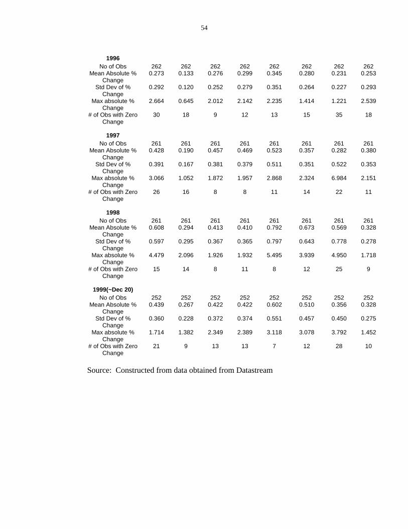
54

1996No of Obs 262 262 262 262 262 262 262 262

Mean Absolute %Change

0.273 0.133 0.276 0.299 0.345 0.280 0.231 0.253

Std Dev of %Change

0.292 0.120 0.252 0.279 0.351 0.264 0.227 0.293

Max absolute %Change

2.664 0.645 2.012 2.142 2.235 1.414 1.221 2.539

# of Obs with ZeroChange

30 18 9 12 13 15 35 18

1997No of Obs 261 261 261 261 261 261 261 261

Mean Absolute %Change

0.428 0.190 0.457 0.469 0.523 0.357 0.282 0.380

Std Dev of %Change

0.391 0.167 0.381 0.379 0.511 0.351 0.522 0.353

Max absolute %Change

3.066 1.052 1.872 1.957 2.868 2.324 6.984 2.151

# of Obs with ZeroChange

26 16 8 8 11 14 22 11

1998No of Obs 261 261 261 261 261 261 261 261

Mean Absolute %Change

0.608 0.294 0.413 0.410 0.792 0.673 0.569 0.328

Std Dev of %Change

0.597 0.295 0.367 0.365 0.797 0.643 0.778 0.278

Max absolute %Change

4.479 2.096 1.926 1.932 5.495 3.939 4.950 1.718

# of Obs with ZeroChange

15 14 8 11 8 12 25 9

1999(~Dec 20)No of Obs 252 252 252 252 252 252 252 252

Mean Absolute %Change

0.439 0.267 0.422 0.422 0.602 0.510 0.356 0.328

Std Dev of %Change

0.360 0.228 0.372 0.374 0.551 0.457 0.450 0.275

Max absolute %Change

1.714 1.382 2.349 2.389 3.118 3.078 3.792 1.452

# of Obs with ZeroChange

21 9 13 13 7 12 28 10

Source: Constructed from data obtained from Datastream

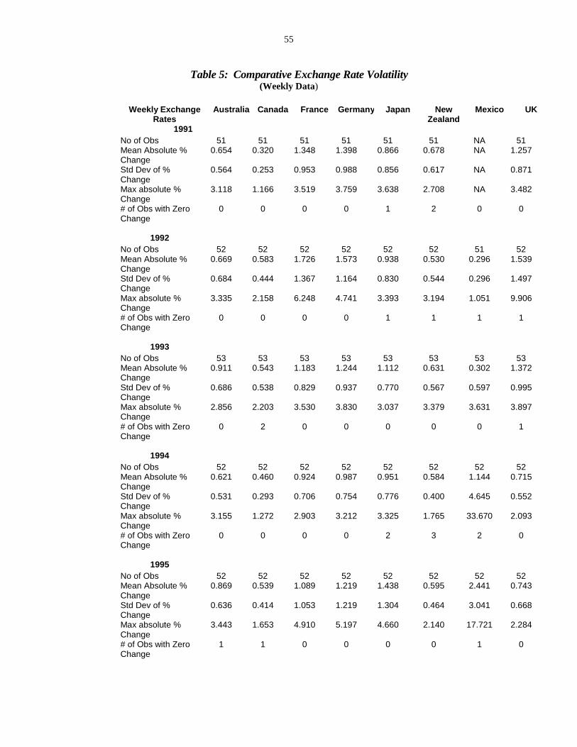
55

Table 5: Comparative Exchange Rate Volatility(Weekly Data)

Weekly ExchangeRates

Australia Canada France Germany Japan NewZealand

Mexico UK

1991No of Obs 51 51 51 51 51 51 NA 51Mean Absolute %Change

0.654 0.320 1.348 1.398 0.866 0.678 NA 1.257

Std Dev of %Change

0.564 0.253 0.953 0.988 0.856 0.617 NA 0.871

Max absolute %Change

3.118 1.166 3.519 3.759 3.638 2.708 NA 3.482

# of Obs with ZeroChange

0 0 0 0 1 2 0 0

1992No of Obs 52 52 52 52 52 52 51 52Mean Absolute %Change

0.669 0.583 1.726 1.573 0.938 0.530 0.296 1.539

Std Dev of %Change

0.684 0.444 1.367 1.164 0.830 0.544 0.296 1.497

Max absolute %Change

3.335 2.158 6.248 4.741 3.393 3.194 1.051 9.906

# of Obs with ZeroChange

0 0 0 0 1 1 1 1

1993No of Obs 53 53 53 53 53 53 53 53Mean Absolute %Change

0.911 0.543 1.183 1.244 1.112 0.631 0.302 1.372

Std Dev of %Change

0.686 0.538 0.829 0.937 0.770 0.567 0.597 0.995

Max absolute %Change

2.856 2.203 3.530 3.830 3.037 3.379 3.631 3.897

# of Obs with ZeroChange

0 2 0 0 0 0 0 1

1994No of Obs 52 52 52 52 52 52 52 52Mean Absolute %Change

0.621 0.460 0.924 0.987 0.951 0.584 1.144 0.715

Std Dev of %Change

0.531 0.293 0.706 0.754 0.776 0.400 4.645 0.552

Max absolute %Change

3.155 1.272 2.903 3.212 3.325 1.765 33.670 2.093

# of Obs with ZeroChange

0 0 0 0 2 3 2 0

1995No of Obs 52 52 52 52 52 52 52 52Mean Absolute %Change

0.869 0.539 1.089 1.219 1.438 0.595 2.441 0.743

Std Dev of %Change

0.636 0.414 1.053 1.219 1.304 0.464 3.041 0.668

Max absolute %Change

3.443 1.653 4.910 5.197 4.660 2.140 17.721 2.284

# of Obs with ZeroChange

1 1 0 0 0 0 1 0

56

1996No of Obs 52 52 52 52 52 52 52 52Mean Absolute %Change

0.632 0.310 0.681 0.697 0.733 0.584 0.548 0.685

Std Dev of %Change

0.602 0.240 0.607 0.650 0.587 0.440 0.500 0.610

Max absolute %Change

2.745 1.267 2.449 2.768 2.285 1.974 2.428 2.643

# of Obs with ZeroChange

4 0 0 0 0 0 0 1

1997No of Obs 52 52 52 52 52 52 52 52Mean Absolute %Change

0.902 0.518 0.902 0.902 1.186 0.744 0.624 0.806

Std Dev of %Change

0.702 0.376 0.694 0.707 1.088 0.732 0.937 0.722

Max absolute %Change

4.028 1.882 3.112 3.030 5.049 2.865 6.331 3.020

# of Obs with ZeroChange

0 0 0 0 1 0 2 1

1998No of Obs 52 52 52 52 52 52 52 52Mean Absolute %Change

1.614 0.685 1.073 1.064 2.122 1.460 1.328 0.826

Std Dev of %Change

1.258 0.628 0.694 0.688 2.328 1.300 1.466 0.641

Max absolute %Change

5.826 2.818 2.880 2.801 14.908 5.587 7.576 2.614

# of Obs with ZeroChange

1 0 0 0 0 1 0 0

1999(~Dec 17)No of Obs 51 51 51 51 51 51 51 51Mean Absolute %Change

1.015 0.553 1.119 1.118 1.598 1.103 0.828 0.768

Std Dev of %Change

0.756 0.465 0.689 0.697 1.191 0.864 0.820 0.523

Max absolute %Change

3.210 1.704 2.859 2.880 5.620 3.787 3.637 2.612

# of Obs with ZeroChange

0 1 0 1 0 2 0 0

I. Source: Constructed from data obtained from Datastream

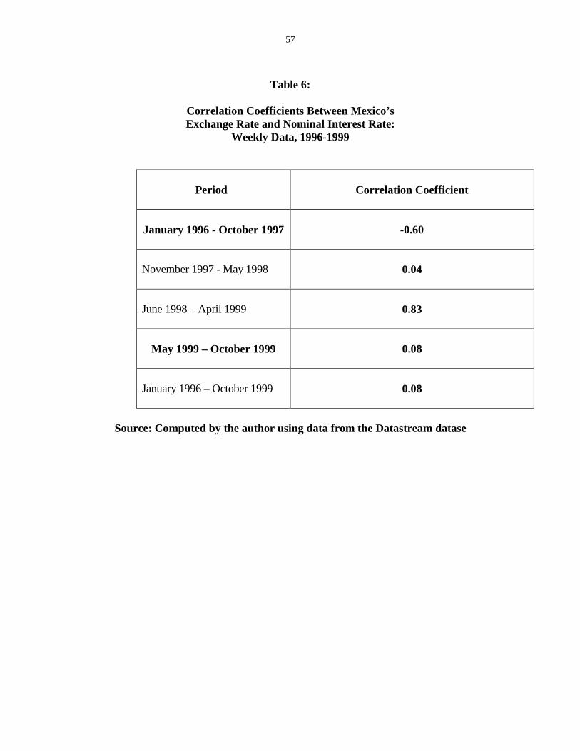
57

Table 6:

Correlation Coefficients Between Mexico’sExchange Rate and Nominal Interest Rate:

Weekly Data, 1996-1999

Period Correlation Coefficient

January 1996 - October 1997 -0.60

November 1997 - May 1998 0.04

June 1998 – April 1999 0.83

May 1999 – October 1999 0.08

January 1996 – October 1999 0.08

Source: Computed by the author using data from the Datastream datase

58

List of Figures

Figure 1: Optimal exit strategy

Figure 2: Tax equivalence of Chile’s URR

Figure 3: Chile and Argentina interest rates

Figure 4: Country vs. currency risk in Argentina

Figure 5: Currency spreads for Argentine deposits

Figure 6: Argentina G-S RER and Actual RER

Figure 7: Panama’s Country Risk Measures

Figure 8: Mexico’s exchange rate

Figure 9: Exchange Rates and Interest Rates in Mexico

59

Costs, B (Private) C (Private)Benefits

C (Social)

B (Social)

T ττττ Time

Figure 1: Optimal Exit: Private and Social Optimal Timing

60

0.00

0.01

0.02

0.03

0.04

0.05

0.06

90 91 92 93 94 95 96 97 98

TAX180 TAX1YR TAX3YRS

Figure 2: Tax Equivalent of Capital Controls:Stay of 180 days, 1 year and 3 years

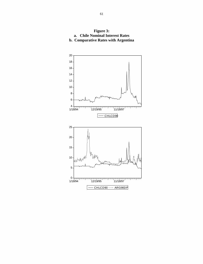
61

Figure 3:a. Chile Nominal Interest Rates

b. Comparative Rates with Argentina

4

6

8

10

12

14

16

18

20

1/18/94 12/19/95 11/18/97

CHLCD90

0

5

10

15

20

25

1/18/94 12/19/95 11/18/97

CHLCD90 ARG90DP

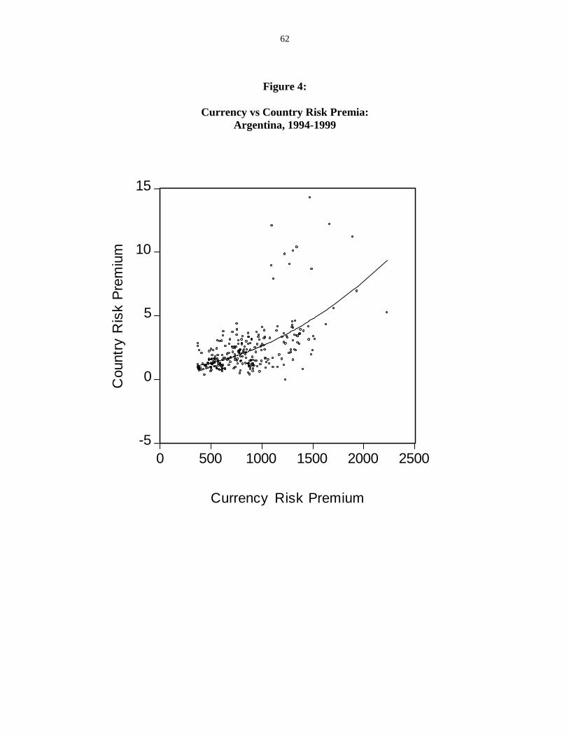
62

Figure 4:

Currency vs Country Risk Premia:Argentina, 1994-1999

-5

0

5

10

15

0 500 1000 1500 2000 2500

Currency Risk Premium

Cou

ntry

Ris

k Pr

emiu

m

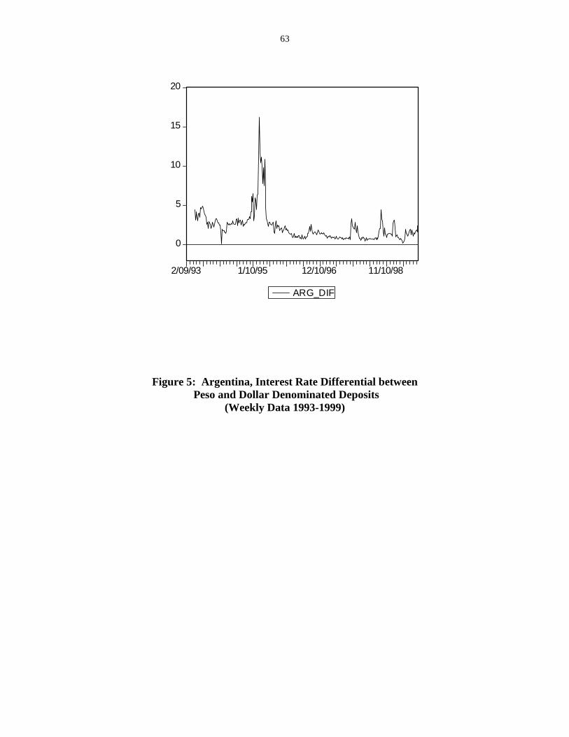
63

Figure 5: Argentina, Interest Rate Differential between Peso and Dollar Denominated Deposits

(Weekly Data 1993-1999)

0

5

10

15

20

2/09/93 1/10/95 12/10/96 11/10/98

ARG_DIF

64

Figure 6: Argentina: Equilibrium and Actual TradeWeighted Real Exchange Rates, 1985-99

(Goldman-Sachs Estimates)

0

100

200

300

400

89 90 91 92 93 94 95 96 97 98 99

ERER RER

65

Figure 7: Panama Brady Bonds Spreads(Daily Data, December 1994-May 1999)

0

200

400

600

800

1000

1200

1400

1600

12/30/94 11/29/96 10/30/98

PFRNSPPIRBSP

PPARSPPPDISP

66

Figure 8: Mexican Peso-U.S. Dollar Exchange Rate.Upper Panel: Spot Exchange Rate

Lower Panel: Rate of Depreciation of the Peso

(Weekly Data, January 1992-October 1999)

2

4

6

8

10

12

1/21/92 12/21/93 11/21/95 10/21/97 9/21/99

MEXSPOT

-10

0

10

20

30

40

1/21/92 12/21/93 11/21/95 10/21/97 9/21/99

MEXDEV

67

Figure 9: Mexico Exchange Rate and 28-dayNominal Interest Rate (Cetes)

(Weekly Data 1994-1999)

2

4

6

8

10

12

0

20

40

60

80

100

2/08/94 1/09/96 12/09/97

MEXSPOT M EXC28C