EXCESSEXCESSEXCESSEXCESS LIQUIDITYLIQUIDITYLIQUIDITYLIQUIDITY ANDANDANDAND INFLATIONINFLATIONINFLATIONINFLATION ININININ CHINA:CHINA:CHINA:CHINA: 2001-20102001-20102001-20102001-2010

by

Bijie Jia

A thesis submitted to the Graduate Faculty ofAuburn University

in partial fulfillment of therequirements for the Degree ofMaster of Science in Economics

Auburn, AlabamaAugust 4, 2012

Keywords: inflation, excess liquidity, real GDP,money supply, price gap, twin surplus

Copyright 2012 by Bijie Jia

Approved by

Henry Thompson, Chair, Professor of EconomicsJohn D. Jackson, Co-Chair, Professor of EconomicsHyeongwoo Kim, Associate Professor of Economics

ii

Abstract

Since the Chinese government administrated the Reform and Opening-up policy designed

toward stimulating China's economy in 1979, China stepped into a period of rapid development.

Accelerated growth of the trade surplus and foreign capital inflows led to the creation of excess

liquidity, which raised inflationary pressures in the economy. In addition to other factors, the

persistence of Chinese inflation may be largely attributable to excess liquidity. This hypothesis is

examined with the ‘price gap measure’ in a regression model that includes the Engle-Granger test for

conintegration. Estimation is based on available quarterly data for the period from 2001 to 2010.

iii

Table of Contents

Abstract...................................................................................................................................................ii

Introduction............................................................................................................................................ 1

CHAPTER 1. Introduction of Twin Surplus in China.........................................................................2

CHAPTER 2. Introduction of Excess Liquidity...................................................................................4

CHAPTER 3. Modeling Inflation as a Function of Excess Liquidity................................................ 7

CHAPTER 4. Other Reasons for Inflation in China..........................................................................12

CHAPTER 5. Conclusion....................................................................................................................13

REFERENCES.....................................................................................................................................14

APPENDIX:......................................................................................................................................... 16

1

InInInIntroductiontroductiontroductiontroduction

The objective of this thesis is to analyze the impact of excess liquidity for the 2001-2010

period on Chinese inflation. This thesis is made up of 5 chapters. Chapter 1 deals with the so-

called "twin surplus" and how it was formed. In Chapter 1 analysis is given to the reasons behind

excess liquidity. Estimation methods then follow in Chapter 2. Through its measurement we

notice that when “too much money chases too few goods” excess liquidity arises. In Chapter 3,

we use Engle-Ganger two-step method to provide evidence that excess liquidity caused inflation.

After modeling the relationship between excess liquidity and inflation in China, in Chapter 4 we

discuss related issues such as the exchange rate, interest rate, and food supply shortage. In

Chapter 5, we draw the conclusion and suggest future research.

2

CHAPTERCHAPTERCHAPTERCHAPTER 1.1.1.1. IntroductionIntroductionIntroductionIntroduction ofofofof TwinTwinTwinTwin SurplusSurplusSurplusSurplus inininin ChinaChinaChinaChina

The Chinese economy has been growing rapidly since the central government put in place

measures towards liberalizing its markets. In 1979, the Chinese government devised the notion of

a Special Economic Zone (SEZ) to be established in the coastal cities; its chief aim was to

stimulate the coastal areas. Foreign investment in SEZs could enjoy tariff reductions and other

preferential policies designed to attract foreign investment.

After the establishment of SEZs, increasing inflows of foreign capital brought along the

development of China's economy, especially in the coastal cities. Over the years, foreign trade

and foreign direct investment (FDI) in China had been expanding rapidly. Because China

typically likes to keep a large foreign exchange reserve, China is facing a twin surplus on both

current and capital accounts in their balance of payments. The current account surplus was $12

billion in 1990 and $249.9 billion in 2006. Since 2004, FDI in China kept increasing annually at a

rate of over $60 billion. China has one of the highest levels of FDI in the world. See Figure 1.

At the beginning of the reformist liberalization policies, Foreign Exchange Reserves (FER)

in China were small; it was even negative at -$1.3 billion in 1980. From 1981 to 1989, China's

FER stayed at a low level. The average FER per year in China during this period was only about

$4.8 billion, but it was still enough to cover a small demand for imports.

By the 1990s, FER increased rapidly because of the development of international trade and

increased inflows of foreign investment. The average annual growth rate during 1991-1996 was

more than 60%. After 2000, because of the acceleration of the trade surplus, FER had been rising

for most of the decade.

3

According to an annual report from the National Bureau of Statistics of China (NBSC), the

rapid growth in imports that began in 2001 was largely due to China’s joining the World Trade

Organization (WTO). During the same period, exports had been expanding at a faster pace than

imports. FER had exceeded $600 billion in 2004. October 2006 was milestone for China when its

FER exceeded $1 trillion.

Finally, after 2006 and until September 2008, foreign exchange reserves in China had

reached $1.9 trillion; in Chinese per capita terms, this is roughly equivalent to $1,500 when

measured against 2008 population levels. By September 2011, FER reached to $3.2 trillion.

China's balance of payments has shown surpluses in both the current and capital accounts. This

has aroused concerns on the part of the Chinese monetary authority about the rise of excess

liquidity and its pressures on consumer price inflation in China.

4

CHAPTERCHAPTERCHAPTERCHAPTER 2.2.2.2. IntroductionIntroductionIntroductionIntroduction ofofofof ExcessExcessExcessExcess LiquidityLiquidityLiquidityLiquidity

Higher exports than imports over years in China make for a trade surplus in the current

account. In addition, low domestic consumption weakens the velocity of money. Increased

Foreign Direct Investment FDI has accelerated the capital inflow in China.

Zhang (2009) notes that accumulation has built up abundant liquidity for China's domestic

market. The Chinese authorities started to express their serious concern that liquidity expansion

in China is out of control, especially when considering the potential transmission from excess

liquidity into inflation.

Let us first consider the quantity equation of money

YPVM ⋅=⋅ . (1)

M denotes stock of money, V denotes the velocity of money, Y represents output, and P is the

price level. Equation (1) describes a relationship that simply states that the stock of money

multiplied by the number of times a money unit that is used for purchasing goods and services (V)

equals real output multiplied by the price level.

If we want to take a further look into how money supply changes affect the economy's

inflation and output, (1) could be rewritten as:

)ln()ln( YPMV ∆=∆ . (2)

Then, we get

pyvm ∆+∆=∆+∆ . (3)

The small letters denote logarithms, and ∆ denotes the first differences. Solving (3) for m∆ , we

can get

5

vpym ∆−∆+∆=∆ . (4)

According to (4), money supply changes equal the output difference plus the price level

difference less the change in the velocity of money.

According to Polleit and Gerdesmeier (2005) for the measurement of excess liquidity, the

price gap measurement for excess liquidity is understandable. They reference the work of

Hallman, Porter, and Small (1991) who define long-term and short-term price level equations.

The long-term price equation as (10) measures the equilibrium price level with the long-run

money velocity and output level; likewise, the short-term (or actual) price level as (11) is based

on the long-run money velocity trend and the potential output level

***tttt yvmp −+= (long-term) (5)

tttt yvmp −+= (short-term). (6)

*tp denotes long-term equilibrium price level, also called potential price level; tp is for the short-

term price level. The difference between tp and *tp is called the price gap,

)()( ***tttttt yyvvpp −+−=− . (7)

The price gap )( *tt pp − could be decomposed into two parts: )( *

tt vv − and )( *tt yy − . If )( *

tt pp − is

negative, it suggests that there will be an upward pressure on inflation in the future. When

tp < *tp , actual price is lower than potential price, it indicates that there will be inflation later;

when tp > *tp , actual price is higher than potential price, so that we will expect a decrease

pressure on inflation in the future.

According to (5),

***ttt ympv +−= (8)

Substitute *v in (7) with (8)

6

)()]([ ****tttttttt yyympvpp −++−−=− (9)

Simplify (9), we get

tttttt ypvmpp −−+=− )( ** . (10)

Equation (10) could be rewritten as

YPMVPP ** // = . (11)

where )( *ttt pvm −+ denotes the money supply and ty denotes the real output. According to (10),

excess liquidity will only happen when there is too much money in the market and too few goods

at the same time. Money is the source of the price gap, and thus the impact on inflation.

YPMV */ is the measurement of excess liquidity here.

Excess liquidity is likely to be an important factor behind the swift increase in inflation that

China has seen in recent years. In conclusion, excess liquidity occurs when current price level is

greater than the potential long-term price level since too much money chases too few goods.

7

CHAPTERCHAPTERCHAPTERCHAPTER 3.3.3.3. ModelingModelingModelingModeling InflationInflationInflationInflation asasasas aaaa FunctionFunctionFunctionFunction ofofofof ExcessExcessExcessExcess LiquidityLiquidityLiquidityLiquidity

Ruffer and Stracca (2006) confirm that excess liquidity was a useful indicator of inflationary

pressure and suggest that it is useful to compare broad money supply (M2) with nominal GDP

(NGDP) to estimate the excess liquidity of a country. They estimate a vector auto-regressive

(VAR) model for 15 countries. Yang (2010) investigates the inflation dynamics and effect of

excess liquidity in China, and revealed that the quasi-money (M2) is the main force behind

China's inflation.

Excess liquidity happens when there is too much money chasing too few goods, which means

excess liquidity occurs when the growth of the money supply is faster than that of GDP. Under

this assumption, we introduce an index of excess liquidity, the Marshallian K index (MK). MK

index is described as the difference of growth of money supply and nominal GDP. We can also

use the ratio of them as (money supply M2)/(nominal GDP) to describe the level of how much

money supply may exceed output ....

However, according to Yang (2010), the standard MK index is an index of current levels, if

we want to explore its long-term effect on inflation, we must do a log-transformation of the MK

index so that we can use the difference between money growth rate and nominal GDP growth rate.

Then, we can see that the relationship between excess liquidity and inflation depends on the

coefficient of the relative change MK index in the model of describing inflation.

The time period of our model is from 2001 to 2010. With reference to the Chinese economy,

however, only the data after 1992 could be used. Yang (2009) pointed out that the market

dominant price mechanism in China worked since 1992 when price reform had completed.

8

The limitation here for using quarterly data is that there may be seasonality. We therefore

need to do make both inflation indicator (CPI) and excess liquidity indicator (ln[(M2)/(GDP)])

de-seasoned and stationary. Before we set up the completed model, consider the explanation of

some important variables in this model.

The excess liquidity indicator, a log-transformation MK index should be expressed as

EL=ln MK index= lnNGDPM 2 . (12)

A main measurement of price is the consumer price index (CPI) that describes the growth rate of

price level as inflation rate. Here, we use the CPI for multiple items for inflation indicators

because we would like to discuss the impact of excess liquidity on general inflation.

We set up a regression model here to test the relationship between inflation and excess

liquidity in China from 2001 to 2010. From Figure 1 we can see the change of inflation based on

consumer price index along with excess liquidity in China from 2001 to 2010 (un-seasoned

quarterly data).

Figure 1 suggests the excess liquidity may systematically affect the consumer price inflation

in China over the most recent decade. A linear regression model will test for the relationship

between excess liquidity and inflation in China. Before that, we apply X12-ARIMA (run by E-

views 7) method to remove the seasonality from both the original CPI and EL data; and then, we

will test for the stationary of these primary variable series.

We use Augmented Dickey–Fuller test ((((ADF) test. ADF test is testing for whether there has

a unit root. If there is a unit root, we accept the null hypothesis that the series is non-stationary,

otherwise we reject the null hypothesis. For CPI, we have its AR(1) process

ttt ecpiaacpi ++= −110 . (13)

9

We express the first difference of CPI for ADF test as

t

p

jjtjtt cpicpiaacpi εβ∑

=−− +∆++=∆

1110 . (14)

Implying the ADF test for tcpi and tcpi∆ respectively, according to the estimation in Table 2:

tcpi is not stationary; tcpi∆ is stationary. Also, the residual term is WN since the ARCH(1) test

in Table 2 is less than 1.6 and Durbin-h is between -1.96 and 1.96.

For EL, we have its AR(1) process

ttt eelaael ++= −110 . (15)

Also, we express the 1st difference of EL for the ADF test

t

p

jjtjtt elelaael εβ∑

=−− +∆++=∆

1110 . (16)

Implying the ADF test for equation (15) and (16) respectively, according to the estimation in

Table 2, tel∆ is stationary. Also, the residual term here is WN.

Since both tcpi∆ and tel∆ are stationary, we set up a simple regression model as inflation is

regressed on excess liquidity

ttt eelaa +∆+= 10π . (17)

tπ is measured by tcpi∆ , tel∆ denotes growth rate of excess liquidity. According to the OLS

estimation (see Table 3), the estimate of (17) is

tt el∆+= 60.260.0π . (18)(0.17) (0.54)

The Engle and Granger’s two-step method generates a regression model based on a long-term

relationship of inflation and excess liquidity.

A simple regression equation based on non-stationary and de-seasoned variables is

10

ttt elaacpi ε++= 10 . (19)

Even if the variables are non-stationary, the linear combination of these two variables may be

stationary, i.e. )0(~1 Ielacpi tt − , and 1a here is unique. If the linear combination here between cpi

and el is stationary, tcpi and tel are cointegrated. Table 4 is the OLS estimation for (19).

The error correction model (ECM) introduces information from (19) into (17). The error

correction regression requires the residual term in (19) is stationary. Check the residual term tε in

(19) with DF test with no constant term in the Engle-Granger regression

ttt ea +=∆ −11εε . (20)

See Table 5, the EG test (t-stat) is significant since t < Tτ = -2.67, and 1α < 0, so that tε is

stationary. There is a presumption that if 1α < 0, the ttst ea ++= −11)1( εε is AR(1) stationary. The

residual term in (20) is WN. So that tcpi and tel in equation (19) are cointegrated.

The residual in equation (19) is not WN but stationary, suggesting that residuals in (19) are

related to each other. Since 1α < 0 in (20) by the EG test, we could derive a error correction

model (EMC)

tcpi∆ = tttt aelaa µεπ ++∆+= −1210 . (21)

Referring to Table 6, the OLS estimation shows the representation of (21) is

128.003.162.0 −−∆+==∆ ttt elcpi επ . (22)(0.28) (0.61) (0.03)

As to the residual term tµ , since DW is approaching to 2 and it passed the ARCH test, it is WN.

Since tπ and tel∆ are cointegrated in this error correction regression as (22), the change of CPI

in (21) not only depends on the difference of EL, but also on the long-run dynamic equilibrium

CPI. The residual term 1−tε brings the relationship among levels into the error correction

regression (21).

11

The long-term impact from excess liquidity on inflation could be measured by the sum of

error correction adjustment and transitory. The error correction adjustment is denoted by the

negative product of coefficient of error correction coefficient in (22) and the coefficient of tel∆ in

(18). It is the adjustment in tel∆ towards to the dynamic equilibrium.

Error correction= -(-0.28)×2.60= 0.73 . (23)(0.03) (0.54) (0.02)

The transitory term is expressed by the coefficient of tel∆ in (22), so that

Transitory = 1.03 . (24)(0.61)

Then, the long-term impact is derived as:

Long-term impact = error correction + transitory

= 0.73 + 1.03 = 1.76 (25)(0.02) (0.61) (0.61)

According to equation (25), the long-term impact from excess liquidity on inflation will be 1.76,

explained as 1 percent increase in the growth rate of excess liquidity may cause 1.76 percent

increase in inflation as a long-term impact. The standard error for the long-term impact derived

with the rule of error propagation 5.22 )( βαγ σσσβαγ +=⇒±= .

12

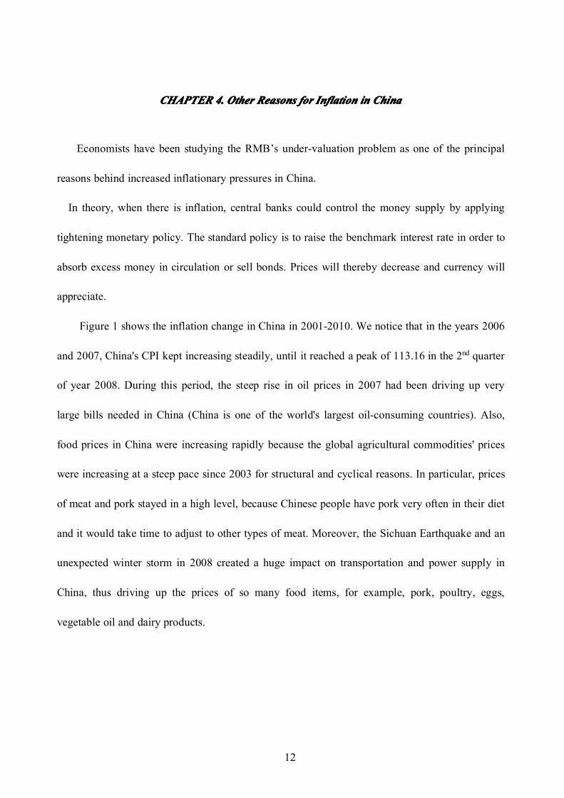
CHAPTERCHAPTERCHAPTERCHAPTER 4.4.4.4. OtherOtherOtherOther ReasonsReasonsReasonsReasons forforforfor InflationInflationInflationInflation inininin ChinaChinaChinaChina

Economists have been studying the RMB’s under-valuation problem as one of the principal

reasons behind increased inflationary pressures in China.

In theory, when there is inflation, central banks could control the money supply by applying

tightening monetary policy. The standard policy is to raise the benchmark interest rate in order to

absorb excess money in circulation or sell bonds. Prices will thereby decrease and currency will

appreciate.

Figure 1 shows the inflation change in China in 2001-2010. We notice that in the years 2006

and 2007, China's CPI kept increasing steadily, until it reached a peak of 113.16 in the 2nd quarter

of year 2008. During this period, the steep rise in oil prices in 2007 had been driving up very

large bills needed in China (China is one of the world's largest oil-consuming countries). Also,

food prices in China were increasing rapidly because the global agricultural commodities' prices

were increasing at a steep pace since 2003 for structural and cyclical reasons. In particular, prices

of meat and pork stayed in a high level, because Chinese people have pork very often in their diet

and it would take time to adjust to other types of meat. Moreover, the Sichuan Earthquake and an

unexpected winter storm in 2008 created a huge impact on transportation and power supply in

China, thus driving up the prices of so many food items, for example, pork, poultry, eggs,

vegetable oil and dairy products.

13

CHAPTERCHAPTERCHAPTERCHAPTER 5.5.5.5. ConclusionConclusionConclusionConclusion

Inflation in China has been a constant macroeconomic problem since the time the reformist

liberalization policy was put into practice by the Chinese government in 1979. With the rapid

increase of foreign exchange reserves and foreign direct investment inflows, including a tightly

controlled exchange rate, excess liquidity has been a problem.

A twin surplus has shown up in China's national accounts and has remained over recent

decades due to a constant international trade surplus and strong rates of inflow of investment.

Even though the Chinese Central Bank tried to raise the benchmark rate 5 times in 2011, it does

not seem to have the desired effect on sterilizing the excess liquidity because it has attracted more

foreign investors to buy bonds in China.

According to the present results there is a significant impact from excess liquidity on inflation.

This positive effect between excess liquidity and inflation is statistically sound and economically

meaningful. Macroeconomic theory suggests inflation is related to money supply and the capacity

of potential output. Results suggest that the price gap as the measurement of excess liquidity is

viable.

14

REFERENCESREFERENCESREFERENCESREFERENCES

Cole, Wayne (2012), Analysis: Oil creeps toward top of Asia's economic worry list, accessed

online.

Coibion, Olivier, Yuriy Gorodnichenko, and Johannes F. Wieland (2010), in the NBER Working

Paper Series, "The Optimal Inflation Rate in New Keynesian Models."

Fleming, J. Marcus (1962). "Domestic financial policies under fixed and floating exchange rates".

IMF Staff Papers 9: 369–379. Reprinted in Cooper, Richard N., ed (1969). International Finance.

New York: Penguin Books.

Friedman (1960), A program for monetary stability, New York: Fordham University Press.

Hallman, Porter, and Small (1991), "Is the Price Level Tied to the M2 Monetary Aggregate in the

Long- Run?", American Economic Review, p. 841-858.

Mundell, Robert A. (1963). "Capital mobility and stabilization policy under fixed and flexible

exchange rates". Canadian Journal of Economic and Political Science 29 (4): 475–485. Reprinted

in Mundell, Robert A. (1968). International Economics. New York: Macmillan.

Polleit, Thorsten and Gerdesmeier, Dieter (2005), "Measures of excess liquidity", HfB – Business

School of Finance & Management, working paper NO.65

Ravallion, Martin (2010), "Price Levels and Economic Growth Making Sense of the PPP

Changes between ICP Rounds", Policy Research Working Paper 5229.

Ruffer and Stracca (2006)," What is global Excess Liquidity, and does it matter?", working paper

series NO.696, European Central Bank

15

Siklos, Pierre L. and Zhang, Yang (2010), "Identifying the Shocks Driving Inflation in China",

Pacific Economic Review P204-223.

Thompson, Henry (2011), International Economics: Global Markets and Competition (3rd

Edition), World Scientific Publishing, Chap.12-13.

Thompson, Henry (2011), "An Introduction to Time Series Regression"

Yiping, Huang, Wang Xun and Hua Xiuping (2010), "What Determine China's Inflation", China

Center for Economics Research, P8

Yang, Jisheng (2010), "Expectation, Excess Liquidity and Inflation Dynamics in China", Higher

Education Press and Springer-Verlag, P412-P418

Zhang, Chengsi (2009), "Excess Liquidity, Inflation and the Yuan Appreciation: What Can China

learn from Recent History", The World Economics, Vol.32, Issue 7, P998-P1018

"Time-series Econometrics: Conintegration and Autoregressive conditional Heteroskedasticity".

Advanced information on the Bank of Sweden Prize in Economic Sciences in Memory of Alfred

Nobel, 8 October 2003

Jia, Yueqing (2010), "Lewis turning point and China's FDI prospects", accessed online.

"VAR Model for Multivariate Time Series", accessed online.

"China's foreign exchange reserves, 1977-2011", accessed online.

"China's Trade Performance", accessed online.

16

APPENDIX:APPENDIX:APPENDIX:APPENDIX:

FIG.1:FIG.1:FIG.1:FIG.1: CPICPICPICPI andandandand ELELELEL inininin China:China:China:China: 2001-20102001-20102001-20102001-2010

* Source: IFS, OECD, Economics Forum of Renmin University (Database), Economics Statistics Database service provided byEconomy Watch.com, Author's calculation.

17

TABLETABLETABLETABLE 1:1:1:1: ADFADFADFADF testtesttesttest forforforfor CPICPICPICPI andandandand ELELELEL

Residual Term

t-stat tcADF + ARCH(1) Durbin-h

tcpi∆ -3.90** -0.78 0.61

tel∆ -4.78*** -0.55 1.56

tcpi -3.06 0.93 3.67

tel 1.40 -0.53 0.45Note: "***","**" and "*" denote significant at 1%, 5% and 10% significant levels respectively. Automatic-based on AIC,maxlags=9.

TABLETABLETABLETABLE 2:2:2:2: OLSOLSOLSOLS estimationestimationestimationestimation forforforfor (20)(20)(20)(20)

0a tel∆

tπ 0.60(0.15)

2.60(1.51)

R2 .27ARCH(1) .13DW1.08

18

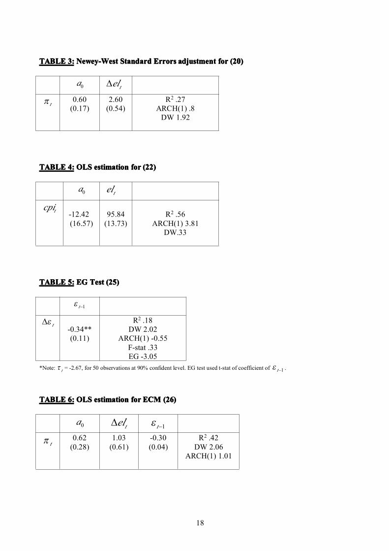
TABLETABLETABLETABLE 3:3:3:3: Newey-WestNewey-WestNewey-WestNewey-West StandardStandardStandardStandard ErrorsErrorsErrorsErrors adjustmentadjustmentadjustmentadjustment forforforfor (20)(20)(20)(20)

0a tel∆

tπ 0.60(0.17)

2.60(0.54)

R2 .27ARCH(1) .8DW 1.92

TABLETABLETABLETABLE 4:4:4:4: OLSOLSOLSOLS estimationestimationestimationestimation forforforfor (22)(22)(22)(22)

0a tel

tcpi-12.42(16.57)

95.84(13.73)

R2 .56ARCH(1) 3.81

DW.33

TABLETABLETABLETABLE 5:5:5:5: EGEGEGEG TestTestTestTest (25)(25)(25)(25)

1−tε

tε∆-0.34**(0.11)

R2 .18DW 2.02

ARCH(1) -0.55F-stat .33EG -3.05

*Note: tτ = -2.67, for 50 observations at 90% confident level. EG test used t-stat of coefficient of 1−tε .

TABLETABLETABLETABLE 6:6:6:6: OLSOLSOLSOLS estimationestimationestimationestimation forforforfor ECMECMECMECM (26)(26)(26)(26)

0a tel∆ 1−tε

tπ 0.62(0.28)

1.03(0.61)

-0.30(0.04)

R2 .42DW 2.06

ARCH(1) 1.01