Embed Size (px)
Citation preview

EXCEPTIONAL ISOMORPHISMS BETWEENCOMPLEMENTS OF AFFINE PLANE CURVES
JÉRÉMY BLANC, JEAN-PHILIPPE FURTER, AND MATTIAS HEMMIG
Abstract. This article describes the geometry of isomorphisms between complementsof geometrically irreducible closed curves in the affine plane A2, over an arbitrary field,which do not extend to an automorphism of A2.
We show that these isomorphisms are quite exceptional. In particular, they occuronly when both curves are isomorphic to open subsets of the affine line A1. Moreover,the isomorphism is uniquely determined by one of the curves, up to left compositionby an automorphism of A2, except in the case where the curve is isomorphic to theaffine line A1 or to the punctured line A1 \ {0}. We also prove that if one curve isisomorphic to a line, then both curves are in fact equivalent to lines. In addition, forany n ∈ N, we construct n (even infinitely many in characteristic 0) pairwise non-equivalent closed embeddings of the punctured line with isomorphic complements. Wethen give a construction that provides a large family of examples of non-isomorphicgeometrically irreducible curves of A2 that have isomorphic complements, answeringnegatively the Complement Problem posed by Hanspeter Kraft [Kra96]. This also givesa negative answer to the holomorphic version of this problem in any dimension n ≥ 2.
Contents
1. Introduction 22. Geometric description of open embeddings A2 \ C ↪→ A2 42.1. Basic properties 42.2. The case of lines 92.3. Embeddings into Hirzebruch surfaces 102.4. Extension to regular morphisms on A2 132.5. Completion with two curves and a boundary 162.6. The case of curves isomorphic to A1 and the proof of Theorem 1 213. Families of non-equivalent embeddings 233.1. A construction using elements of SL2(k[y]) 243.2. Curves isomorphic to A1 \ {0} 254. Non-isomorphic curves with isomorphic complements 294.1. A geometric construction 294.2. Getting explicit formulas 345. Related questions 385.1. Providing higher dimensional counterexamples 385.2. The holomorphic case 39Appendix: The case of P2 40References 44The authors gratefully acknowledge support by the Swiss National Science Foundation Grant "Bi-
rational Geometry" PP00P2_128422 /1 and by the French National Research Agency Grant "BirPol",ANR-11-JS01-004-01.
1

2 JÉRÉMY BLANC, JEAN-PHILIPPE FURTER, AND MATTIAS HEMMIG
1. Introduction
In the Bourbaki Seminar Challenging problems on affine n-space [Kra96], HanspeterKraft gives a list of eight basic problems related to the affine n-spaces. The sixth one isthe following:
Complement Problem. Given two irreducible hypersurfaces E,F ⊂ An and anisomorphism of their complements, does it follow that E and F are isomorphic?
Recently, Pierre-Marie Poloni gave a negative answer to the problem for any n ≥ 3[Pol16]. The construction is given by explicit formulas. There are examples where bothE and F are smooth, and examples where E is singular, but F is smooth. This articledeals with the case of dimension n = 2. The situation is much more rigid than indimension n ≥ 3, as we discuss in Theorem 1.
We recall that two curves C,D ⊂ A2 are equivalent if there is an automorphismof A2 that sends one onto the other. Note that equivalent curves are isomorphic. Avariety defined over a field k is called geometrically irreducible if it is irreducible over thealgebraic closure of k (it will then be reduced, as all curves in the sequel). A line in A2
is a closed curve of degree 1.
Theorem 1. Let k be any field. Let C ⊂ A2 be a geometrically irreducible closed curveand let ϕ : A2 \ C '−→ A2 \D be an isomorphism, where D ⊂ A2 is also a closed curve.
If ϕ does not extend to an automorphism of A2, then both C and D are isomorphic toopen subsets of A1. More precisely, there are isomorphisms
C ' Spec(k[t,1
P]) and D ' Spec(k[t,
1
Q])
for some square-free polynomials P,Q ∈ k[t] that have the same number of roots in k,and the same number of roots in the algebraic closure k.
Moreover, the following holds:(1) If C is isomorphic to A1, then both C and D are equivalent to lines.(2) If C is not isomorphic to A1 or to A1 \{0}, then the isomorphism ϕ (which does not
extend to an automorphism of A2) is uniquely determined by C, up to left compositionby an automorphism of A2. In particular, there are at most two equivalence classesof curves in A2 with complements isomorphic to A2 \ C.
Corollary. If the ground field k is algebraically closed, and
ϕ : A2 \ C '−→ A2 \Dis an isomorphism between the complements of two irreducible plane closed curves C,D ⊂A2 which does not extend to an automorphism of A2, then there exist two finite subsetsF,G of the affine line A1 of the same cardinality such that C is isomorphic to A1 \ Fand D is isomorphic to A1 \G.
If F contains at least 2 points, then ϕ is uniquely determined by C, up to left compo-sition by an automorphism of A2. The equivalence class of D is uniquely determined byC, except when F contains exactly one point.
Corollary. Let C ⊂ A2 be a singular, geometrically irreducible closed curve and ϕ : A2 \C
'−→ A2 \ D an isomorphism, for some closed curve D. Then ϕ extends to an auto-morphism of A2.

EXCEPTIONAL ISOMORPHISMS BETWEEN COMPLEMENTS OF AFFINE PLANE CURVES 3
The second corollary shows in particular that the Complement Problem for n = 2 hasa positive answer if one of the curves is singular, contrary to the case where n ≥ 3, aspointed out before. It is also very different to the case of P2, where there exist non-isomorphic irreducible curves with isomorphic complements [Bla09, Theorem 1], butwhere all examples are necessarily singular (see Proposition A.1 below).
Theorem 1 also shows that the Complement Problem for n = 2 has a positive answerif the curve is not rational (which is an easy observation, see Corollary 2.8 below) butmore generally when it is not isomorphic to an open subset of A1. For instance, thecircle x2 + y2 = 1 over R is a smooth rational affine curve which is not isomorphic to anopen subset of A1.
In addition, Theorem 1 gives strong restrictions on isomorphisms between comple-ments of curves: if C is not isomorphic to A1 \ {0} and there exists an isomorphismϕ : A2 \C '−→ A2 \D that does not extend to an automorphism of A2, then ϕ is unique(up to left composition by an automorphism of A2), hence the class of D is unique too.This is again quite different to the case of dimension n ≥ 3 where there are infinitelymany hypersurfaces E ⊂ An, up to equivalence, that have isomorphic complements[Pol16, Lemma 3.1]. It is also different to the case of P2, where we can find algebraicfamilies of non-equivalent curves of P2 that have isomorphic complements (and thusinfinitely many if k is infinite). This follows from a construction made in [Cos12], seeCorollary A.3 below.
All tools necessary to obtain the rigidity result (Theorem 1) are developped in Sec-tion 2. The proof is then achieved at the end of the section. Our second statement isthe following existence result, which shows the optimality of Theorem 1.
Theorem 2. Let k be any field.(1) There exists a closed curve C ⊂ A2, isomorphic to A1 \ {0}, whose complement
A2 \ C admits infinitely many open embeddings A2 \ C ↪→ A2 into the affine plane,up to automorphisms of A2. Moreover, the set of equivalence classes of curves withthis property is infinite.
(2) For each integer n ≥ 1 there exist pairwise non-equivalent curves C1, . . . , Cn ⊂ A2,all isomorphic to A1 \ {0}, such that all open surfaces A2 \ C1, . . . , A2 \ Cn areisomorphic. Moreover, if char(k) = 0, we can find an infinite sequence of pairwisenon-equivalent curves Ci ⊂ A2, i ∈ N, such that all open surfaces A2 \Ci, i ∈ N, areisomorphic.
(3) For each polynomial f ∈ k[t] of degree ≥ 1, there exist two non-equivalent closedcurves C,D ⊂ A2, both isomorphic to Spec(k[t, 1
f]), such that the open surfaces A2\C
and A2 \D are isomorphic. Moreover, the set of such pairs of closed embeddings ofSpec(k[t, 1
f]) is infinite, up to equivalence.
The proof of Theorem 2, mainly via explicit constructions, is made in Section 3.
We then give counterexamples to the Complement Problem in dimension 2, over anyfield:
Theorem 3. For any ground field k, there exist two geometrically irreducible closedcurves C,D ⊂ A2 which are not isomorphic but whose complements A2 \ C and A2 \D
4 JÉRÉMY BLANC, JEAN-PHILIPPE FURTER, AND MATTIAS HEMMIG
are isomorphic. Furthermore, these two curves can be chosen of degree 7 if the fieldadmits more than 2 elements and of degree 13 if the field has 2 elements.
The proof of this result is detailed in Section 4. We first give a geometric constructionin Lemma 4.1. Then, we show in Proposition 4.2 that, for each polynomial P ∈ k[t] ofdegree d ≥ 1 and each λ ∈ k with P (λ) 6= 0, this construction yields two closed curvesC,D ⊂ A2 of degree d2 − d + 1 such that A2 \ C and A2 \ D are isomorphic and suchthat the following isomorphisms hold:
C ' Spec(
k[t,1
P])and D ' Spec
(k[t,
1
Q]), where Q(t) = P
(λ+
1
t
)· tdeg(P ).
The proof of Theorem 3 follows by providing an appropriate pair (P, λ) for each field. Thecase of infinite fields is quite easy. Indeed, if k is infinite and P ∈ k[t] is a polynomial withat least 3 roots in k, then Spec(k[t, 1
P]) and Spec(k[t, 1
Q]) are not isomorphic, for a general
element λ ∈ k (Lemma 4.5). This shows that the isomorphism type of counterexamplesto the Complement Problem is as large as possible.
We finish this introduction by giving some easy implications of Theorem 3, detailedin Section 5:
(i) The negative answer to the Complement Problem for n = 2 directly yields anegative answer for any n ≥ 3 (Lemma 5.1): Our construction gives, for each n ≥ 3,two geometrically irreducible smooth closed hypersurfaces E,F ⊂ An which are notisomorphic but whose complements An \ E and An \ F are isomorphic (Corollary 5.2).All the hypersurfaces provided this way are isomorphic to An−2×C for some open subsetC ⊂ A1. This does not allow to give singular examples like the ones of [Pol16], but givesa different type of examples.
(ii) Choosing k = C, our construction also gives families of closed complex curvesC,D ⊂ C2 such that C2 \C and C2 \D are biholomorphic (because they are isomorphicas algebraic varieties) but C and D are not biholomorphic (Lemma 5.3). This directlyprovides, for each n ≥ 2, the existence of algebraic hypersurfaces E,F ⊂ Cn whichare complex manifolds that are not biholomorphic but have biholomorphic complements(Corollary 5.4). This is, to our knowledge, the first family of such examples, and yieldsthe answer to a problem asked in [Pol16]. Note that in the counterexamples of [Pol16],if both hypersurfaces are smooth, then they are always biholomorphic (even if they arenot isomorphic as algebraic varieties).
The authors thank Hanspeter Kraft, Lucy Moser-Jauslin and Pierre-Marie Poloni forinteresting discussions during the preparation of this article.
2. Geometric description of open embeddings A2 \ C ↪→ A2
In the sequel, we work over an arbitrary field k. When we say rational, resp. iso-morphic, we mean k-rational, resp. k-isomorphic. The word geometrically rational orgeometrically irreducible refers to the extension to the algebraic closure k, as usual.
2.1. Basic properties. In order to study isomorphisms between affine surfaces, it isoften interesting to see the affine surfaces as open subsets of projective surfaces and to seethen the isomorphisms as birational maps between the projective surfaces. Recall thata rational map ϕ : X 99K Y between smooth projective irreducible surfaces is defined

EXCEPTIONAL ISOMORPHISMS BETWEEN COMPLEMENTS OF AFFINE PLANE CURVES 5
on an open subset U ⊂ X such that F = X \ U is finite. If C is an irreducible curveof the surface X, its image is defined by ϕ(C) := ϕ(C \ F ). We then say that C iscontracted by ϕ if ϕ(C) is a point. The aim of this section is to establish Lemma 2.7,that we use often in the sequel. Its proof relies on some easy results that we recall before:Lemmas 2.2, 2.4, 2.6 and Corollary 2.5.
Example 2.1. The morphismA2 ↪→ P2
(x, y) 7→ [x : y : 1]
gives an isomorphism A2 '−→ P2 \ LP2 , where LP2 ⊂ P2 denotes the “line at infinity”given by z = 0. The above embedding of A2 into P2 will be often used in the sequel,and called the standard embedding.
With this standard embedding, every line of A2, given by an equation ax + by = cwhere a, b, c are elements of k and a, b are not both zero, is the restriction of a line of P2,given by the equation ax+ by = cz, and distinct from LP2 .
Lemma 2.2. Let ϕ : X 99K Y be a birational map between two projective surfaces andassume that ϕ restricts to an isomorphism U
'−→ V where U ⊂ X and V ⊂ Y are twoopen subsets.(1) Any geometrically irreducible closed curve Γ ⊂ X\U is sent either to a point of Y \V
or to a curve contained in Y \ V .(2) Assume that η : Z → X and π : Z → Y are birational morphisms that yield a minimal
resolution of ϕ as shown on the following diagram:
Zη
uu
π
))Xϕ // Y
U?�
OO
' // V?�
OO
Then, we have η−1(U) = π−1(V ).
Proof. The morphisms η and π are obtained by blowing up the base-points of ϕ andϕ−1 respectively, which are by assumption not contained in U and V respectively. Thisyields point (2), which in turn yields point (1). �
Definition 2.3. For each birational map ϕ : P2 99K P2, one defines Jϕ ⊂ P2 to be thereduced curve given by the union of all irreducible k-curves contracted by ϕ.
Lemma 2.4. Let ϕ : P2 99K P2 be a birational map.(1) The curve Jϕ is defined over k, i.e. is the zero locus of a homogeneous polynomial
f ∈ k[x, y, z].(2) We have an isomorphism P2 \Jϕ → P2 \Jϕ−1. Moreover, the number of k-irreducible
components of Jϕ and Jϕ−1 are equal.
Proof. (1): If char(k) = 0 one could choose f to be the Jacobian determinant associatedto ϕ. This does not work in positive characteristic as the Jacobian determinant can bezero. We then do as follows: we write ϕ as ϕ : [x : y : z] 7→ [s0(x, y, z) : s1(x, y, z) :s2(x, y, z)], where s0, s1, s2 ∈ k[x, y, z] are homogeneous polynomials of the same degree

6 JÉRÉMY BLANC, JEAN-PHILIPPE FURTER, AND MATTIAS HEMMIG
without common factor and do the same with ϕ−1 : [x : y : z] 7→ [q0(x, y, z) : q1(x, y, z) :q2(x, y, z)]. We then do the composition and obtain q0(s0, s1, s2) = xA, q1(s0, s1, s2) =yA, q2(s0, s1, s2) = zA, for some polynomial A ∈ k[x, y, z] and observe that Jϕ is thezero locus of A. Indeed, the polynomial A is zero along an irreducible k-curve if andonly if this curve is sent by ϕ onto a base-point of ϕ−1.
(2) We take a minimal resolution of ϕ, which yields a commutative diagram
Xη
uu
π
))P2 ϕ // P2
where η and π are birational morphisms, the morphism η, resp. π, being the sequenceof blow-ups of the k-base-points of ϕ, resp. ϕ−1.
We can now work over k, forgetting the subfield k. Computing the Picard rank of X,we see that η and π contract the same number of irreducible curves of X. Let n be thisnumber. We then denote by E ⊂ X, resp. F ⊂ X, the union of the n irreducible curvescontracted by η, resp. π. The map ϕ restricts then to an isomorphism
P2 \ η(E ∪ F )'−→ P2 \ π(E ∪ F )
Let us observe that η(E ∪ F ) = η(F ). Since η(E) consists of finitely many points, itsuffices to show that these are contained in the curves of η(F ). Each point p of η(E)corresponds to a connected component of E, which contains at least one (−1)-curveE ⊂ E. The curve E is not contracted by π, by minimality, hence sent by π onto a curveπ(E) ⊂ P2, of self-intersection ≥ 1. This implies that E intersects F and thus p ∈ η(F ).One similarly gets π(E ∪ F ) = π(E), and obtains that ϕ restricts to an isomorphism
P2 \ η(F )'−→ P2 \ π(E).
It remains to observe that η(F ) is a closed curve of P2 (in general not irreducible)and that each of its k-component is contracted by ϕ, so η(F ) = Jϕ. Similarly, onegets π(E) = Jϕ−1 . Moreover, the number of k-irreducible components of η(F ) is equalto the number of k-irreducible components of F \ E, which is equal to the number ofk-irreducible components of E \ F . This achieves the proof. �
Corollary 2.5. Let ϕ : P2 \ Γ ↪→ P2 be an open embedding, where Γ is a closed k-curve,which is a finite union of r distinct irreducible closed k-curves of P2. Then, there is aunique closed k-curve ∆ ⊂ P2 such that ϕ(P2 \Γ) = P2 \∆, and ∆ is also a finite unionof r distinct irreducible closed k-curves of P2.
Proof. Let ϕ : P2 99K P2 be the birational map induced by ϕ. Lemma 2.4 implies thatJϕ ⊂ Γ, that Jϕ and Jϕ−1 are finite unions of s ≤ r irreducible closed distinct k-curvesof P2, and that ϕ induces an isomorphism P2 \ Jϕ
'−→ P2 \ Jϕ−1 .If s = r, the proof is over. Otherwise, Γ′ = Γ \ Jϕ is a closed k-curve of P2 \ Jϕ,
which is the union of r− s irreducible closed k-curves. The closed k-curve ∆′ = ϕ(Γ′) ofP2 \ Jϕ−1 is again the union of r− s irreducible closed k-curves. The result follows with∆ = ∆′ ∪ Jϕ−1 . �
Lemma 2.6. Let ϕ : X 99K Y be a birational map between two smooth projective surfaces(all defined over k), such that every irreducible k-curve contracted by ϕ is defined over

EXCEPTIONAL ISOMORPHISMS BETWEEN COMPLEMENTS OF AFFINE PLANE CURVES 7
k. Then, each base-point of ϕ−1 is k-rational and each irreducible k-curve contracted byϕ is k-rational.
Proof. We argue by induction on the number of base-points of ϕ−1. If there is nosuch base-point, there is nothing to show. Otherwise, let C be an irreducible k-curvecontracted by ϕ to a point p of Y . Since C is defined over k, so is its image, i.e. p isk-rational (the generic point of C is defined over k and is sent onto the k-point p). Letπ : Y ′ → Y be the blow-up at p and let ϕ′ = π−1 ◦ ϕ : X 99K Y ′. The base-points of(ϕ′)−1 coincide with the base-points of ϕ−1 from which the point p is removed. Moreover,the curves contracted by ϕ′ are also contracted by ϕ, and if a curve is contracted by ϕand not contracted by ϕ′, then it is sent by ϕ′ onto the exceptional divisor π−1(p) andis thus k-rational. Therefore, the result follows by induction. �
In the sequel, we will frequently use the following observation:
Lemma 2.7. Let C ⊂ A2 be a geometrically irreducible closed curve and let ϕ : A2\C ↪→A2 be an open embedding. Then, there exists a geometrically irreducible closed curveD ⊂ A2 such that ϕ(A2 \ C) = A2 \ D. Denote by C and D the closures of C andD in P2, denote as in Example 2.1 by LP2 = P2 \ A2 the line at infinity and denoteby ϕ : P2 99K P2 the birational map induced by ϕ. Then, one of the following threealternatives holds:(1) We have ϕ(C) = D. Then, the map ϕ extends to an automorphism of A2 = P2 \LP2
sending C onto D.(2) We have ϕ(C) = LP2. Then, the curve D is a line of A2, i.e. D is a line of P2 and
ϕ extends to an isomorphism A2 = P2 \ LP2'−→ P2 \D, that sends C onto LP2 \D.
In particular, C is equivalent to a line via an automorphism of A2.(3) The map ϕ contracts the curve C to a k-point of P2. Then, the curve C (and
therefore, also the curve C) is a rational curve (i.e. is k-birational to P1).
Proof. The restriction of ϕ to P2 \ (LP2 ∪C) = A2 \C gives the open embedding ϕ : A2 \C ↪→ A2 ↪→ P2. By Corollary 2.5, we obtain an isomorphism P2 \ (LP2 ∪C)
'−→ P2 \∆,for some k-curve ∆ ⊂ P2, which is the union of two k-irreducible closed curves of P2.Since LP2 is included in ∆, there exists an irreducible closed k-curve D of A2 such that∆ = LP2 ∪D. As a conclusion, ϕ induces an isomorphism
P2 \ (LP2 ∪ C)'−→ P2 \ (LP2 ∪D).
It follows that ϕ(A2 \C) = A2 \D. The equality D = A2 \ϕ(A2 \C) proves us that thecurve D is defined over k and is therefore geometrically irreducible. By Lemma 2.2, oneof the following three alternatives holds:
(1) We have ϕ(C) = D. Hence, ϕ induces an automorphism of A2 = P2 \ LP2
(Lemma 2.4).(2) We have ϕ(C) = LP2 . Then, ϕ induces an isomorphism P2\LP2
'−→ P2\D (againby Lemma 2.4). Since the Picard group of P2 \ Γ is isomorphic to Z/ deg(Γ)Z,for each irreducible curve Γ, the curve D must be a line of P2.
(3) The map ϕ contracts the curve C to a point of P2. Then, by Lemma 2.6, thispoint is necessary a k-point and the curve C is k-rational. �

8 JÉRÉMY BLANC, JEAN-PHILIPPE FURTER, AND MATTIAS HEMMIG
Corollary 2.8. Let C ⊂ A2 be a geometrically irreducible closed curve. If C is notrational (i.e. not k-birational to P1), then every open embedding A2 \ C ↪→ A2 extendsto an automorphism of A2.
Proof. Follows from Lemma 2.7 and the fact that cases (2)-(3) only occur when C isrational. �
Remark 2.9. It follows from Corollary 2.8 that the group of automorphisms of A2 \ C,where C is a non-rational geometrically irreducible curve, is the subgroup of Aut(A2)preserving C. By [BS15, Theorem 2], this group is finite (and in particular conjugate toa subgroup of GL2(k) if char(k) = 0, see for instance [Kam79]).
We find it interesting to observe that case (3) of Lemma 2.7 only occurs when Cintersects LP2 in at most two k-points, even if this will not be used in the sequel.
Corollary 2.10. If C ⊂ A2 is a closed geometrically irreducible curve such that Cintersects LP2 = P2\A2 in at least three k-points, then every open embedding A2\C ↪→ A2
extends to an automorphism of A2.
Proof. We can assume that k = k. Suppose, for contradiction, that the extensionϕ : P2 99K P2 does not restrict to an automorphism of A2. By Lemma 2.7, the curve Cis contracted by ϕ (because C is not equivalent to a line, so (2) is impossible). We recallthat ϕ restricts to an isomorphism A2 \C = P2 \ (LP2 ∪C)
'−→ A2 \D = P2 \ (LP2 ∪D)(Lemma 2.7) and that C ⊂ Jϕ ⊂ LP2 ∪ C, Jϕ−1 ⊂ LP2 ∪ D, where Jϕ, Jϕ−1 have thesame number of irreducible components (Lemma 2.4). We take a minimal resolution ofϕ, which yields a commutative diagram
Xη
uu
π
))P2 ϕ // P2.
We first observe that the strict transforms LP2 , C ⊂ X of LP2 , C by η intersect in at mostone point. Indeed, otherwise the curve LP2 is not contracted by π, because π contractsC, and sent onto a singular curve, which has then to be D. We get Jϕ = C, Jϕ−1 = LP2
and get an isomorphism P2 \ C → P2 \ LP2 , impossible because C has degree at least 3.Secondly, the fact that LP2 , C ⊂ X intersect in at most one point implies that η blows
up all points of C ∩ LP2 except at most one. Since Jϕ−1 ⊂ D ∪ LP2 , there are at mosttwo (−1)-curves contracted by η. But LP2 and C intersect in at least three points, so weobtain exactly two proper base-points of ϕ, corresponding to exactly two (−1)-curvesE1, E2 ⊂ X contracted to two points p1, p2 ∈ C ∩ LP2 by η. Moreover, Jϕ−1 = D ∪ LP2
so Jϕ = C ∪ LP2 (Lemma 2.4). Writing E ′i = η−1(pi) \ Ei, we find that π contractsF = E ′1 ∪ E ′2 ∪ C ∪ LP2 .
Let us show that Ei · F ≥ 2, for i = 1, 2, which will imply that π(Ei) is a singularcurve for i = 1, 2, and yield a contradiction since E1, E2 are sent by π onto LP2 and D.As Ei ∪ E ′i = η−1(pi), it is a tree of rational curves, which intersects both C and LP2
since pi ∈ C ∩LP2 . If E ′i is empty, then Ei · C ≥ 1 and Ei · LP2 ≥ 1, whence Ei ·F ≥ 2 aswe claimed. If E ′i is not empty, then Ei · E ′i ≥ 1. The only possibility to get Ei · F ≤ 1would thus be that Ei · E ′i = 1, Ei · C = Ei · LP2 = 0. The equality Ei · E ′i = 1 impliesthat E ′i is connected, and Ei · C = Ei · LP2 = 0 yields C ·E ′i ≥ 1 and LP2 ·E ′i ≥ 1. Since
EXCEPTIONAL ISOMORPHISMS BETWEEN COMPLEMENTS OF AFFINE PLANE CURVES 9
LP2 and C intersect in a point disjoint from E ′i, this implies that F contains a loop andthus cannot be contracted. �
Remark 2.11. In case (3) of Lemma 2.7, it is possible that C intersects the line LP2
in two points, as it is the case in most of our examples (see for example Lemma 3.2or Lemma 3.9). The case of one point is of course also possible (see for instanceLemma 2.13(1)).
We will also need the following basic algebraic observation.
Lemma 2.12. Let f ∈ k[x, y] be a polynomial, irreducible over k, and let C ⊂ A2 be thecurve given by f = 0. Then, the ring of functions on A2 \ C and its subset of invertibleelements are equal to
O(A2 \ C) = k[x, y, f−1] ⊂ k(x, y), O(A2 \ C)∗ = {λfn | λ ∈ k∗, n ∈ Z}.In particular, every automorphism of A2 \ C exchanges the fibres of the morphism
A2 \ C → A1 \ {0}given by f .
Proof. The field of rational functions of A2 \ C is equal to k(x, y). We can write anyelement of this field as u/v, where u, v ∈ k[x, y] are coprime polynomials, v 6= 0. Therational function is regular on A2 \ C if and only if v does not vanish on any k-pointof A2 \ C. This means that v = λfn, for some λ ∈ k∗, n ≥ 0. This provides thedescription of O(A2 \C) and O(A2 \C)∗. The last remark follows from the fact that thegroup O(A2 \C)∗ is generated by k∗ and one single element g, if and only if this elementg is equal to λf±1 for some λ ∈ k∗. �
2.2. The case of lines. Lemma 2.7 shows that one needs to study isomorphisms A2 \C
'−→ A2 \ D, which extend to birational maps of P2 that contract the curve C to apoint. One can ask whether this point can be a point of A2 (and thus would be containedin D) or belongs to the boundary line LP2 = P2 \ A2. As we will show (Corollary 2.19),the first possibility only occurs in a very special case, namely when C is equivalent to aline by an automorphism of A2. The case of lines is special for this reason, and is treatedseparately here.
Lemma 2.13. Let C ⊂ A2 be the line given by x = 0.(1) The group of automorphisms of A2 \ C is given by:
Aut(A2 \ C) = {(x, y) 7→ (λx±1, µxny + s(x, x−1)) | λ, µ ∈ k∗, n ∈ Z, s ∈ k[x, x−1]}.(2) Every open embedding A2 \ C ↪→ A2 is equal to ψα, where α ∈ Aut(A2 \ C) and
ψ : A2 \ C ↪→ A2 extends to an automorphism of A2. In particular, the complementof its image, i.e. the complement of ψα(A2 \ C) = ψ(A2 \ C), is a curve equivalentto a line by an automorphism of A2.
Proof. To prove (1), we first observe that each transformation (x, y) 7→ (λx±1, µxny +s(x, x−1)) actually yields an automorphism of A2 \C. Then, we only need to show thatall automorphisms of A2 \C are of this form. An automorphism of A2 \C corresponds toan automorphism of k[x, y, x−1], which sends x onto λx±1, where λ ∈ k∗ (Lemma 2.12).Applying the inverse of (x, y) 7→ (λx±1, y), we can assume that x is fixed. We are left

10 JÉRÉMY BLANC, JEAN-PHILIPPE FURTER, AND MATTIAS HEMMIG
with an R-automorphism of R[y], where R is the ring k[x, x−1]. Such an automorphism isof the form y 7→ ay+b, where a ∈ R∗, b ∈ R. Indeed, if the maps y 7→ p(y) and y 7→ q(y)are inverses of each other, the equality y = p(q(y)) proves us that deg p = deg q = 1.This yields the desired form.
To prove (2), we use Lemma 2.7 and write ϕ as an isomorphism A2\C '−→ A2\D whereD is a geometrically irreducible closed curve, and only need to see that D is equivalentto a line by an automorphism of A2. We write ψ = ϕ−1, choose an equation f = 0for D (where f ∈ k[x, y] is an irreducible polynomial over k) and get an isomorphismψ∗ : O(A2 \ C) = k[x, y, x−1]→ O(A2 \D) = k[x, y, f−1] that sends x to λf±1 for someλ ∈ k∗ (Lemma 2.12). We can thus write ψ as (x, y) 7→ (λf(x, y)±1, g(x, y)f(x, y)n),where n ∈ Z and g ∈ k[x, y]. Replacing ψ with its composition with the automorphism(x, y) 7→ ((λ−1x)±1, y((λ−1x)±1)−n) of A2 \ C, we can assume that ψ is of the form(x, y) 7→ (f(x, y), g(x, y)). If g is equal to a constant ν ∈ k modulo f , we apply theautomorphism (x, y) 7→ (x, (y−ν)x−1) and decrease the degree of g. After finitely manysteps we obtain an isomorphism A2\D → A2\C of the form ψ0 : (x, y) 7→ (f(x, y), g(x, y))where g is not a constant modulo f . The image of D by ψ0 is then dense in C, whichimplies that ψ0 extends to an automorphism of A2 sending D onto C (Lemma 2.7). �
2.3. Embeddings into Hirzebruch surfaces. We will not only need embeddings ofA2 into P2 but also other embeddings of A2 into smooth projective surfaces, and inparticular into Hirzebruch surfaces. These surfaces play a natural role in the studyof automorphisms of A2 (and of images of curves by these automorphisms), as we candecompose every automorphism of A2 into small links between such surfaces and thenstudy how the singularities at infinity of the curves behave under these small links (seefor instance [BS15]).
Example 2.14. For n ≥ 1, the n-th Hirzebruch surface Fn is
Fn = {([a : b : c], [u : v]) ∈ P2 × P1 | bvn = cun}
and the projection πn : Fn → P1 yields a P1-bundle structure on Fn.Let Sn, Fn ⊂ Fn be the curves given by [1 : 0 : 0] × P1 and v = 0, respectively. The
morphismA2 ↪→ Fn
(x, y) 7→ ([x : yn : 1], [y : 1])
gives an isomorphism A2 ∼→ Fn\(Sn ∪ Fn).
We recall the following classical easy result:
Lemma 2.15. For each n ≥ 1, the projection πn : Fn → P1 is the unique P1-bundlestructure on Fn, up to automorphism of P1. The curve Sn is the unique irreduciblek-curve of Fn of self-intersection −n, and we have (Fn)2 = 0.
Proof. Since Fn\(Sn ∪ Fn) is isomorphic to A2, whose Picard group is trivial, one hasPic(Fn) = ZFn + ZSn. Moreover, Fn is a fibre of πn and Sn is a section, so (Fn)2 = 0and Fn · Sn = 1. Denoting by S ′n ⊂ Fn the section given by a = 0, one finds that S ′n isequivalent to Sn + nFn, by computing the divisor of a
c.
Since Sn and S ′n are disjoint, this yields 0 = Sn ·(Sn+nFn) = (Sn)2+n, so (Sn)2 = −n.

EXCEPTIONAL ISOMORPHISMS BETWEEN COMPLEMENTS OF AFFINE PLANE CURVES 11
To get the result, it suffices to show that an irreducible k-curve C ⊂ Fn not equal toSn or to a fibre of πn has self-intersection at least equal to n. This will show in particularthat a general fibre of any morphism Fn → P1 is equal to a fibre of πn, since this one hasself-intersection 0. We write C = kSn + lFn for some k, l ∈ Z. Since C 6= Sn we have0 ≤ C · Sn = l − nk. Since C is not a fibre, it intersects every fibre, so 0 < Fn · C = k.This yields l ≥ nk > 0 and C2 = −nk2 + 2kl = kl + k(l − nk) ≥ kl ≥ nk2 ≥ n. �
Lemma 2.16. Let C ⊂ A2 be a geometrically irreducible closed curve. Then, thereexists an integer n ≥ 1 and an isomorphism ι : A2 '−→ Fn\(Sn ∪ Fn) such that theclosure of ι(C) in Fn is a curve Γ which satisfies one of the following two possibilities:(1) Γ · Fn = 1 and Γ ∩ Fn ∩ Sn = ∅.(2) Γ · Fn ≥ 2 and the following assertions hold:
(a) If n = 1, then 2mp(Γ) ≤ Γ · F1 for {p} = S1 ∩ F1, and mr(Γ) ≤ Γ · S1 for eachr ∈ F1(k).
(b) If n ≥ 2, then 2mr(Γ) ≤ Γ · Fn for each r ∈ Fn(k).Furthermore, in Case (1), the curve C is equivalent to a curve given by an equation ofthe form
a(y)x+ b(y) = 0,
where a, b ∈ k[y] are coprime polynomials such that a 6= 0 and deg b < deg a. Moreover,the following assertions are equivalent:
(i) The polynomial a is constant;(ii) The curve C is equivalent to a line by an automorphism of A2 ;
(iii) The curve C is isomorphic to A1;(iv) Γ · Sn = 0.
Proof. Let us take any fixed isomorphism ι : A2 '−→ Fn\(Sn ∪ Fn) for some n ≥ 1, anddenote by Γ the closure of ι(C).
We first assume that we have Γ · Fn = 1. This is equivalent to saying that Γ is asection of πn. We can furthermore assume that Γ ∩ Fn ∩ Sn = ∅, as otherwise we blowup the point Fn∩Sn, contract the curve Fn, change the embedding to Fn+1 and decreasefrom one unity the intersection number of Γ with Sn at the point Sn ∩Fn. After finitelymany steps we get Γ ∩ Fn ∩ Sn = ∅, i.e. we are in Case (1).
If Γ · Fn = 0, then Γ is a fibre of πn : Fn → P1. Let ψ be the unique automorphism ofA2 such that ι ◦ ψ is the standard embedding of A2 into Fn of Example 2.14. Then, thecurve C is equivalent to the curve ψ−1(C), which has equation y = λ, for some λ ∈ k.This proves that C is equivalent to the line y = λ, and thus to the line x = λ, sent bythe standard embedding onto a curve satisfying the conditions (1).
It remains to consider the case where Γ · Fn ≥ 2. If Γ satisfies (2), we are done.Otherwise, we have a k-point p ∈ Fn satisfying one of the following two possibilities:
(a) n = 1, mp(Γ) > Γ · S1, and p ∈ F1.(b) 2mp(Γ) > Γ · Fn and either n ≥ 2 or n = 1 and p ∈ S1 ∩ F1.
We will replace the isomorphism A2 '−→ Fn\(Sn ∪ Fn) with another one, where thesingularities of the curve Γ either decrease (all multiplicities have not changed, except onemultiplicity which has decreased) or stay exactly the same (as usual, the multiplicitiestaken into account do not only concern the proper points of Fn but also the infinitely

12 JÉRÉMY BLANC, JEAN-PHILIPPE FURTER, AND MATTIAS HEMMIG
near points). Moreover, the case where the multiplicities stay the same is only in (a),which cannot appear two consecutive times. We then get the result after finitely manysteps.
In case (a), we observe that the inequality mp(Γ) > Γ · S1 joined with the inequalityΓ · S1 ≥ (Γ · S1)p ≥ mp(Γ) · mp(S1) implies that p /∈ S1. We can then choose p to bea k-point of F1 \ S1 of maximal multiplicity and denote by τ : F1 → P2 the birationalmorphism contracting S1 to a k-point q ∈ P2, observe that τ(F1) is a line through q,that τ(Γ) is a curve of multiplicity Γ · S1 at q and of multiplicity mp(Γ) > Γ · S1 atp′ = τ(p) ∈ τ(F1). Moreover, p′ is a k-point of τ(F1) of maximal multiplicity on thatline. Denote by τ ′ : F′1 → P2 the birational morphism which is the blow-up at p′. Let S ′1be the exceptional fibre of τ ′, F ′1 the strict transform of τ(F1) and Γ′ the strict transformof τ(Γ). We then replace the isomorphism A2 '−→ F1 \ (S1 ∪ F1) with the analogousisomorphism A2 '−→ F′1 \ (S ′1 ∪ F ′1) and get
∀ r ∈ F ′1, mr(Γ′) ≤ Γ′ · S ′1 = mp(Γ).
Hence, (a) is not anymore possible. Moreover, the singularities of the new curve Γ′ haveeither decreased or stayed the same: Indeed, the multiplicities of the singular points ofτ(Γ) are the same as those of Γ, plus one point of multiplicity Γ · S1. Similarly, themultiplicities of the singular points of τ(Γ) are the same as those of Γ′, plus one point ofmultiplicitymp(Γ). Of course, we do not really get a singular point if the multiplicity is 1.Therefore, the singularities of the new curve remain the same if and only if mp(Γ) = 1and Γ · S1 = 0. The situation is illustrated below in a simple example (which satisfiesmp(Γ) = 3 > Γ · S1 = 2).
F1
S1
Γ
p
τ−→τ(F1)
p′
τ(Γ)
q
τ ′←−
F ′1
S′1
Γ′
In case (b), we denote by κ : Fn 99K Fn′ the birational map that blows up the point p andcontracts the strict transform of Fn. Call q the point to which the strict transform of Fnis contracted. We have κ = πq ◦ (πp)
−1, where πp, resp. πq, are blow-ups of the point pof Fn, resp. the point q of Fn′ . The drawing below illustrates the situation in a case wheren′ = n−1. The composition of ι with κ provides a new isomorphism A2 → Fn′\(Sn′∪Fn′),where Sn′ is the image of Sn and Fn′ is the curve corresponding to the exceptional divisorof p. Note that Fn′ is a fibre of the P1-bundle π′ : Fn′ → P1 corresponding to π′ = πn◦κ−1,and that Sn′ is a section, of self-intersection −n′, where n′ = n+1 if p ∈ Sn and n′ = n−1if p /∈ Sn. Hence, since n ≥ 2 or n = 1 and {p} = Sn∩Fn, we get that (Sn′)
2 = −n′ < 0,and obtain a new isomorphism ι′ : A2 '−→ Fn′\(Sn′ ∪ Fn′). The singularity of the newcurve Γ′ at the point q is equal to Γ ·Fn−mp(Γ), which is strictly smaller than mp(Γ) byassumption. Moreover 2mp(Γ) > Γ · Fn ≥ 2, which implies that p was indeed a singular

EXCEPTIONAL ISOMORPHISMS BETWEEN COMPLEMENTS OF AFFINE PLANE CURVES 13
point of Γ.
Fn
Sn
Γ
p
πp←−−
π−1p (p)
π−1q (q)
πq−→
Fn′
Sn′
Γ′
q
Finally, we must now prove the last statement of our lemma, which concerns Case (1).Let ψ be the unique automorphism of A2 such that ι ◦ ψ is the standard embeddingof A2 into Fn of Example 2.14. Then, replacing ι by ι ◦ ψ and C by the equivalentcurve ψ−1(C), we may assume that ι : A2 '−→ Fn\(Sn ∪ Fn) is the standard embedding.This being done, the restriction of πn : Fn → P1 to A2 is (x, y) → [y : 1]. The fibresof πn, equivalent to Fn being given by y = cst, the degree in x of the equation of C isequal to Γ · Fn (this can be done for instance by extending the scalars to k and takinga general fibre). Since Γ · Fn = 1, the equation is of the form xa(y) + b(y) for somepolynomials a, b ∈ k[y], a 6= 0. Since C is geometrically irreducible, the polynomials aand b are coprime. There exist (unique) polynomials q, b ∈ k[x] such that b = aq + b
with deg b < deg a. Then, changing the coordinates by applying (x, y) 7→ (x + q(y), y),one may furthermore assume that deg b < deg a.
Let us prove that points (i)-(iv) are equivalent. The implications (i) ⇒ (ii) ⇒ (iii)are obvious. We then prove (iii)⇒ (iv)⇒ (i).
(iii) ⇒ (iv): We recall that Γ is a section of πn : Fn → P1, so that we have isomor-phisms Γ ' P1 and Γ \ Fn ' A1. The fact that C = Γ \ (Fn ∪ Sn) ' A1 implies thatC ∩ (Sn \ Fn) is empty. Since Γ ∩ Fn ∩ Sn = ∅ by assumption, one gets Γ · Sn = 0.
(iv)⇒ (i): We use the open embedding
A2 ↪→ Fn(u, v) 7→ ([1 : uvn : u], [v : 1]).
The preimages of Γ and Sn by this embedding are the curves of equations a(v)+b(v)u = 0and u = 0. Hence Γ · Sn = 0 implies that a has no k-root and thus is a constant. �
2.4. Extension to regular morphisms on A2. The following proposition, is the prin-cipal tool in the proof of Lemma 2.23, Corollary 2.24 and Proposition 2.26, which them-selves give the main part of Theorem 1.
Proposition 2.17. Let C ⊂ A2 be a geometrically irreducible closed curve, not equiva-lent to a line by an automorphism of A2, and let ϕ : A2 \C ↪→ A2 be an open embedding.Then, there exists an open embedding ι : A2 ↪→ Fn, for some n ≥ 1, such that the rationalmap ι ◦ϕ extends to a regular morphism A2 → Fn, and such that ι(A2) = Fn \ (Sn ∪Fn)(where Sn and Fn are as in Example 2.14).
Proof. By Lemma 2.7, ϕ(A2 \C) = A2 \D for some geometrically irreducible curve D. Ifϕ extends to an automorphism of A2 sending C onto D, the result is obvious, by takingany isomorphism ι : A2 '−→ Fn \ (Fn ∪ Sn), so we can assume that ϕ does not extendto an automorphism of A2. Lemma 2.13 implies, since C is not equivalent to a lineby an automorphism of A2, that the same holds for D. Moreover, Lemma 2.7 implies

14 JÉRÉMY BLANC, JEAN-PHILIPPE FURTER, AND MATTIAS HEMMIG
that the extension of ϕ−1 to a birational map A2 99K P2, via the standard embeddingA2 ↪→ P2, contracts the curve D (or D) to a k-point of P2. In particular, it does notsend D birationally onto C or onto LP2 .
We choose an open embedding ι : A2 ↪→ Fn given by Lemma 2.16, which comes froman isomorphism ι : A2 '−→ Fn\(Sn ∪ Fn), such that the closure ι(D) in Fn is a curve Γwhich satisfies one of the two possibilities (1)-(2) of Lemma 2.16.
We want to show that the open embedding ι ◦ ϕ : A2 \ C ↪→ Fn extends to a regularmorphism on A2. Using the standard embedding of A2 into P2, one gets a birationalmap ψ : P2 99K Fn and needs to show that all base-points of this map are contained inLP2 . We take as usual a minimal resolution of ψ and obtain a commutative diagram
Xη
ssπ
++A2 � � std // P2 ψ // Fn A2? _ιoo
A2 \ C8 X
kk
ϕ
'// A2 \D.
& �
33
Note that ψ restricts to an isomorphism P2 \ (LP2 ∪C)'−→ Fn \ (Fn ∪ Sn ∪ Γ) and that
by Lemma 2.2(2) we have the equality η−1(LP2 ∪C) = π−1(Fn∪Sn∪Γ). As we observedbefore, the map ψ−1 : Fn 99K P2 contracts Γ = ι(D) to a k-point, and thus does not sendΓ birationally onto C or LP2 . The possible curves contracted by ψ are LP2 , C and thepossible curves contracted by ψ−1 are Γ, Fn, Sn. Since all these are defined over k, allbase-points of ψ, ψ−1 are defined over k (Lemma 2.6).
We suppose, for contradiction, that ψ has a base-point q in A2 = P2 \ LP2 , whichmeans that one (−1)-curve Eq ⊂ X is contracted by η to q. This curve is the exceptionaldivisor of a base-point infinitely near to q but not necessarily of q. The minimality ofthe resolution implies that π does not contract Eq, so π(Eq) is a curve of Fn contractedby ψ−1 to q, which belongs to {Γ, Fn, Sn}.
We observe that ψ has also a base-point p in LP2 . Indeed, otherwise the strict trans-form of LP2 would have self-intersection 1 on X: It would then not be contracted by π,and would be sent onto a curve of self-intersection ≥ 1, which belongs to {Γ, Fn, Sn} byLemma 2.2. As (Fn)2 = 0 and (Sn)2 = −n ≤ −1, LP2 is sent onto Γ by ψ. But Γ is notsent birationally onto LP2 by ψ−1, as we observed before. This contradiction gives us abase-point p in LP2 and a (−1)-curve Ep ⊂ X contracted by η to p and not contractedby π. As above, this curve is the exceptional divisor of a base-point infinitely near to p,but not necessarily of p. Again, π(Ep) belongs to {Γ, Fn, Sn}.
We thus have at least two of the curves Γ, Fn, Sn that correspond to (−1)-curves of Xcontracted by η.
We suppose first that Sn corresponds to a (−1)-curve of X contracted by η. The factthat (Sn)2 = −n ≤ −1 implies that n = 1 and that π does not blow up any point of Sn.As there is another (−1)-curve of X contracted by η, the two curves are disjoint on X,and thus also disjoint on F1, since π does not blow up any point of S1. The other curveis then Γ (since F1 · S1 = 1), and Γ · S1 = 0. If moreover Γ · F1 = 1 (condition (1)of Lemma 2.16), then the contraction F1 → P2 of S1 sends Γ onto a line of P2, whichcontradicts the fact that D ⊂ A2 is not equivalent to a line. If Γ ·F1 ≥ 2, then condition(2) of Lemma 2.16 implies that mr(Γ) ≤ Γ · S1 = 0 for each r ∈ F1(k). Hence, theintersection of Γ with F1 (which is not empty since Γ · F1 ≥ 2) only consists of points

EXCEPTIONAL ISOMORPHISMS BETWEEN COMPLEMENTS OF AFFINE PLANE CURVES 15
not defined over k, which are therefore not blown up by π. The strict transforms Γ andF1 on X satisfy then Γ · F1 = Γ · F1 ≥ 2. As Γ is contracted by η, the image η(F1) is asingular curve and is then equal to C. This contradicts the fact that ψ contracts C toa point.
The remaining case is when Sn does not correspond to a (−1)-curve ofX contracted byη, which implies that {π(Ep), π(Eq)} = {Fn,Γ}, or equivalently that {Ep, Eq} = {Fn, Γ},where Fn and Γ denote the strict transforms of Fn and Γ on X. Since (Fn)2 = 0 and(Fn)2 = −1, there exists exactly one point r ∈ Fn (and no infinitely near points) blownup by π, which is then a k-point (as all base-points of π are defined over k). We obtain
mr(Γ) = Γ · Fn ≥ 1 and Γ ∩ Fn = {r},
since Fn and Γ are disjoint on X (and because Γ · Fn ≥ 1, as Γ satisfies one of the twoconditions (1)-(2) of Lemma 2.16).
We now prove that π−1(r) and π−1(Sn) are two disjoint connected sets of rationalcurves which intersect the two curves Fn and Γ, i.e. the two curves Ep and Eq. To showthis, it suffices to prove that r /∈ Sn and that Sn · Γ ≥ 1. Suppose first that Γ · Fn = 1(condition (1) of Lemma 2.16). Since Γ∩Fn∩Sn = ∅, we get r ∈ Fn \Sn. The inequalityΓ ·Sn > 0 is provided by the fact that D is not equivalent to a line by an automorphismof A2 (see again condition (1) of Lemma 2.16 and the equivalence between (ii) and (iv)given in that case). Suppose now that Γ · Fn ≥ 2. As mr(Γ) = Γ · Fn ≥ 2, we have2mr(Γ) > Γ · Fn, which implies that n = 1, r ∈ Fn \ Sn and 2 ≤ mr(Γ) ≤ Γ · Sn (seeagain possibility (2) of Lemma 2.16).
We finish by observing that, since η(Eq) = q ∈ P2 \ LP2 and η(Ep) = p ∈ LP2 , anyconnected set of curves of η−1(LP2 ∪ C) which touches the two curves Eq and Ep hasto contain the strict transform C of C. Remembering that π−1(r) and π−1(Sn) areincluded into π−1(Fn∪Sn∪Γ) = η−1(LP2 ∪C), this contradicts the fact that π−1(r) andπ−1(Sn) are two disjoint connected sets of rational curves which intersect the two curvesFn and Γ. �
A direct corollary of Proposition 2.17 is the following, which shows that only smoothcurves C ⊂ A2 are interesting to study. This follows also from Lemma 2.23 below. Sincethe proof of Lemma 2.23 is more involved, we prefer to first explain the simpler argumentthat shows how the smoothness follows from Proposition 2.17.
Corollary 2.18. Let C ⊂ A2 be a geometrically irreducible curve. If C is not smooth,then every open embedding ϕ : A2 \ C ↪→ A2 extends to an automorphism of A2.
Proof. By Lemma 2.7, ϕ(A2 \ C) = A2 \D for some geometrically irreducible curve D.We apply Proposition 2.17 and obtain an open embedding ι : A2 ↪→ Fn, for some n ≥ 1,such that the rational map ι◦ϕ extends to a regular morphism A2 → Fn. Embedding A2
into P2, we get a birational map ψ : P2 99K Fn which is regular on A2. In particular, thesingular points of C are not blown up in the minimal resolution of ψ. So, the curve C isnot contracted. Since ψ restricts to an isomorphism P2\(LP2∪C)
'−→ Fn\(Fn∪Sn∪D),Lemma 2.2 shows us that C is sent onto a singular curve of Fn which has to be Fn, Sn orD. Since Fn and Sn are smooth, this singular curve must be D. Lemma 2.7 then showsthat ϕ extends to an automorphism of A2. �

16 JÉRÉMY BLANC, JEAN-PHILIPPE FURTER, AND MATTIAS HEMMIG
Another direct consequence of Proposition 2.17 is the following result, which showsthat in Case (3) of Lemma 2.7, the point where C is contracted to lies in A2 only in avery special situation:
Corollary 2.19. Let C ⊂ A2 be a geometrically irreducible closed curve and let ϕ : A2 \C ↪→ A2 be an open embedding. If the extension of ϕ to P2 contracts the curve C(or its closure) to a point of A2, then there exist automorphisms α, β of A2 and anendomorphism ψ : A2 → A2 of the form (x, y) 7→ (x, xny), where n ≥ 1 is an integer,such that ϕ = αψβ. In particular, C ⊂ A2 is equivalent to a line, via β.
Proof. By Lemma 2.7, ϕ(A2 \ C) = A2 \D for some geometrically irreducible curve D.Denote by ϕ−1 : A2 99K A2 the birational transformation which is the inverse of ϕ. SinceC is contracted by ϕ to a point of A2, it is not possible to find an open embeddingι : A2 ↪→ Fn, for some n ≥ 1, such that the birational map ι ◦ ϕ−1 actually defines aregular morphism A2 → Fn. By Proposition 2.17, this implies that D is equivalent to aline by an automorphism of A2. Hence, the same holds for C, by Lemma 2.13. Applyingautomorphisms of A2 at the source and the target, we can then assume that C and Dare equal to the line x = 0. By Lemma 2.13(1), the map ϕ is of the form (x, y) 7→(λx, µxny+ s(x)), where λ, µ ∈ k∗, n ≥ 1 and s ∈ k[x] is a polynomial. We then observethat ϕ = αψ, where α is the automorphism of A2 given by (x, y) 7→ (λx, µy + s(x)) andψ is the endomorphism of A2 given by (x, y) 7→ (x, xny). �
Corollary 2.19 also gives a simple proof of the following characterisation of birationalendomorphisms of A2 that contract only one geometrically irreducible curve, alreadyobtained by Daniel Daigle in [Dai91, Theorem 4.11].
Corollary 2.20. Let C ⊂ A2 be a geometrically irreducible closed curve and let ϕ bea birational endomorphism of A2 which restricts to an open embedding A2 \ C ↪→ A2.Then, the following assertions are equivalent:
(i) The endomorphism ϕ contracts the curve C.(ii) The endomorphism ϕ is not an automorphism.
(iii) There exist automorphisms α, β of A2 and an endomorphism ψ : A2 → A2 of theform (x, y) 7→ (x, xny), where n ≥ 1 is an integer, such that ϕ = αψβ.
Proof. (iii) ⇒ (ii): Follows from the fact that, for each n ≥ 1, the map ψ : (x, y) 7→(x, xny) is a birational endomorphism of A2 which is not an automorphism, as its inverseψ−1 : (x, y) 7→ (x, x−ny) is not regular.
(ii) ⇒ (i): Denote by ϕ : P2 99K P2 the birational map induced by ϕ. Since ϕ is anendomorphism of A2 which is not an automorphism, the cases (1)-(2) of Lemma 2.7 arenot possible. Hence, we are in case (3): C is contracted by ϕ to a point of P2, which isnecessarily in A2 since ϕ(A2) ⊂ A2.
(i)⇒ (iii): Follows from Corollary 2.19. �
2.5. Completion with two curves and a boundary. The following technical lemma(Lemma 2.23) is used to prove Corollary 2.24 and Proposition 2.26, which yield almostall statements of Theorem 1.
Definition 2.21. Let X be a smooth projective surface. A reduced closed curve C ⊂ Xis a k-forest of X if C is a finite union of closed curves C1, . . . , Cn, all k-isomorphic to
EXCEPTIONAL ISOMORPHISMS BETWEEN COMPLEMENTS OF AFFINE PLANE CURVES 17
P1 and if each singular point of C is a k-point lying on exactly two components Ci, Cjintersecting transversally. We moreover ask that C does not contain any loop. If C isconnected, we say that C is a k-tree.
Remark 2.22. If η : X → Y is a birational morphism between smooth projective surfacessuch that all base-points of η−1 are defined over k, then the exceptional curve of η(union of curves contracted) is a k-forest E ⊂ X. Moreover, the strict transform andthe preimage of any k-forest of Y is a k-forest of X. The preimage of a k-tree is a k-tree.
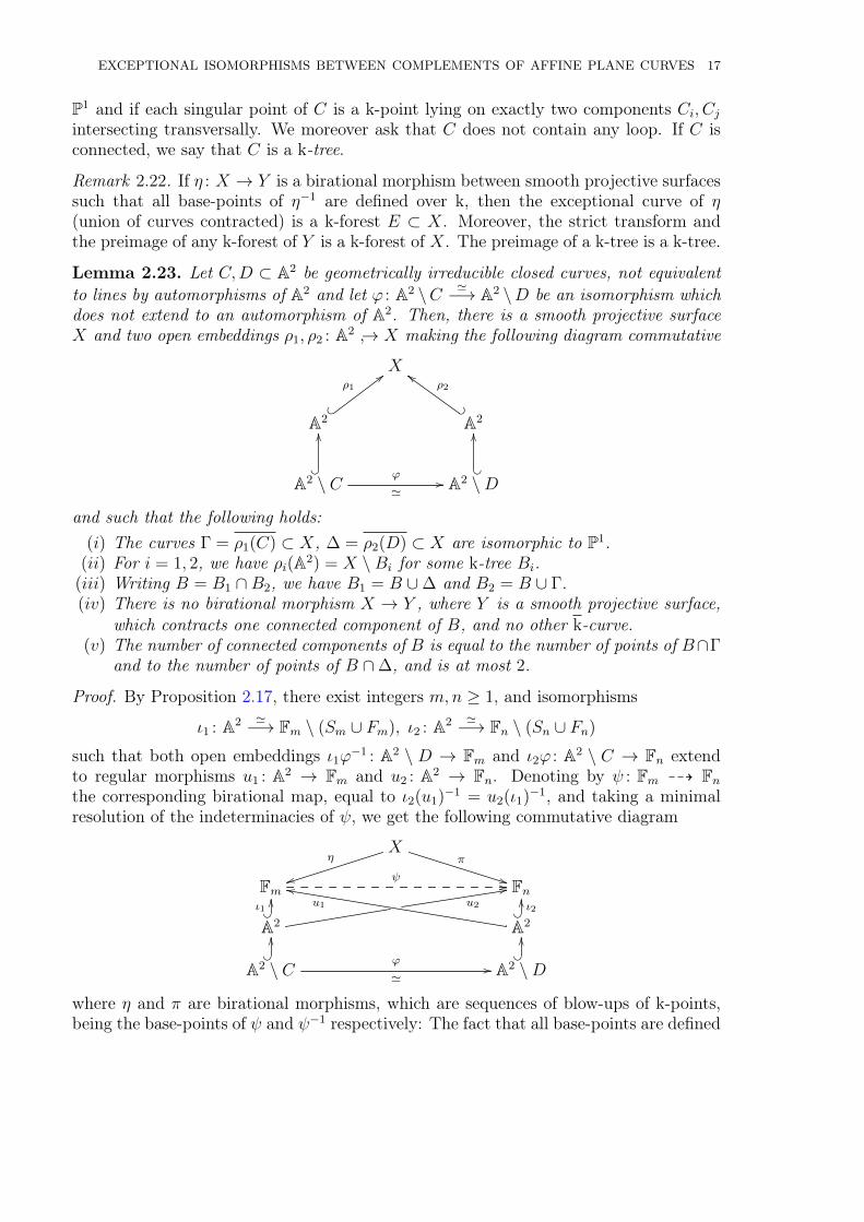
Lemma 2.23. Let C,D ⊂ A2 be geometrically irreducible closed curves, not equivalentto lines by automorphisms of A2 and let ϕ : A2 \C '−→ A2 \D be an isomorphism whichdoes not extend to an automorphism of A2. Then, there is a smooth projective surfaceX and two open embeddings ρ1, ρ2 : A2 ↪→ X making the following diagram commutative
X
A2-
ρ1;;
A21 Q
ρ2cc
A2 \ C?�
OO
ϕ
'// A2 \D
� ?
OO
and such that the following holds:(i) The curves Γ = ρ1(C) ⊂ X, ∆ = ρ2(D) ⊂ X are isomorphic to P1.
(ii) For i = 1, 2, we have ρi(A2) = X \Bi for some k-tree Bi.(iii) Writing B = B1 ∩B2, we have B1 = B ∪∆ and B2 = B ∪ Γ.(iv) There is no birational morphism X → Y , where Y is a smooth projective surface,
which contracts one connected component of B, and no other k-curve.(v) The number of connected components of B is equal to the number of points of B∩Γ
and to the number of points of B ∩∆, and is at most 2.
Proof. By Proposition 2.17, there exist integers m,n ≥ 1, and isomorphisms
ι1 : A2 '−→ Fm \ (Sm ∪ Fm), ι2 : A2 '−→ Fn \ (Sn ∪ Fn)
such that both open embeddings ι1ϕ−1 : A2 \ D → Fm and ι2ϕ : A2 \ C → Fn extendto regular morphisms u1 : A2 → Fm and u2 : A2 → Fn. Denoting by ψ : Fm 99K Fnthe corresponding birational map, equal to ι2(u1)−1 = u2(ι1)−1, and taking a minimalresolution of the indeterminacies of ψ, we get the following commutative diagram
Xη
tt
π
**Fmψ // Fn
A2?�
ι1OO
u2
22
A2?�ι2OO
u1
ll
A2 \ C?�
OO
ϕ
'// A2 \D?�
OO
where η and π are birational morphisms, which are sequences of blow-ups of k-points,being the base-points of ψ and ψ−1 respectively: The fact that all base-points are defined

18 JÉRÉMY BLANC, JEAN-PHILIPPE FURTER, AND MATTIAS HEMMIG
over k follows from Lemma 2.6, because the irreducible k-curve contracted by ψ andψ−1 are all defined over k, since they are equal to Sn, Fn, Sm, Fm, u1(D) or u2(C). Sinceu1, u2 are regular on A2, the base-points of ψ, resp. ψ−1, belong to Fm ∪ Sm ⊂ Fm,resp. Fn ∪ Sn ⊂ Fn. In particular, we get two open embeddings
ρ1 = η−1ι1 : A2 ↪→ X, ρ2 = π−1ι2 : A2 ↪→ X
such that ρ2ϕ = ρ1 (or more precisely ρ2ϕ = ρ1|A2\C). We have ρ1(A2) = X \ B1 andρ2(A2) = X \ B2, where B1 := η−1(Sm ∪ Fm) and B2 := π−1(Sn ∪ Fn) are k-trees (seeRemark 2.22).
The restriction of ψ gives an isomorphism Fm \ (Sm ∪Fm ∪ ι1(C))'−→ Fn \ (Sn ∪Fn ∪
ι2(D)) (which corresponds to ϕ). By Lemma 2.2(2), the following equality holds:
η−1(Sm ∪ Fm ∪ ι1(C)) = π−1(Sn ∪ Fn ∪ ι2(D)).
The left-hand side is equal to B1 ∪ Γ, where Γ = ρ1(C) ⊂ X is the strict transform ofι1(C) ⊂ Fm by η and the right-hand side is equal to B2 ∪ ∆, where ∆ = ρ2(D) ⊂ X
is the strict transform of ι2(D) ⊂ Fn by π. The fact that ϕ does not extend to anautomorphism of A2 implies that B1 6= B2, whence ∆ 6= Γ. Writing B := B1 ∩ B2, theequality B1 ∪ Γ = B2 ∪∆ yields:
B2 = B ∪ Γ and B1 = B ∪∆ (with Γ = ρ1(C),∆ = ρ2(D) ⊂ X).
In particular, since B1, B2 are two k-trees, Γ and ∆ are isomorphic to P1 (over k) andintersect transversally B in a finite number of k-points. We have then found the surfaceX together with the embeddings ρ1, ρ2, satisfying conditions (i)–(ii)–(iii). We will thenmodify X if needed, in order to also get (iv)–(v).
The number of connected components of B is equal to the number of points of B ∩Γ,and of B ∩∆: This follows from the fact that B ∪ Γ and B ∪∆ are k-trees. Let us alsorecall that each point of B ∩ Γ, or of B ∩∆, is a k-point, as said before.
Suppose that the number of connected components of B is r ≥ 3, and let us showthat at least r−2 connected components of B are contractible (in the sense that there isa birational morphism X → Y , where Y is a smooth projective rational surface, whichcontracts one component of B and no other k-curve). To show this, we first observe thatΓ intersects r distinct curves of B. Since Γ is one of the irreducible components of B2 =π−1(Sn ∪ Fn), we can decompose π as π2 ◦ π1 where π1(Γ) is an irreducible componentof (π2)−1(Sn ∪ Fn) intersecting exactly two other irreducible components R1, R2, andsuch that all points blown up by π1 are infinitely near points of π1(Γ) \ (R1 ∪R2). Thisproves that we can contract at least r − 2 connected components of B.
If one connected component of B is contractible, there exists a morphism X → Y ,where Y is a smooth projective rational surface, which contracts this component of B,and no other curve. Since the component intersects ∆ transversally in one point, andalso Γ in one point, we can replace X with Y , ρ1, ρ2 with their compositions with themorphism X → Y and still have conditions (i)–(ii)–(iii). After finitely many steps,condition (iv) is satisfied. By the observation made before, the number of connectedcomponents of B, after this being done, is at most 2, giving then (v). �
Corollary 2.24. Let C,D ⊂ A2 be geometrically irreducible closed curves and let ϕ : A2\C
'−→ A2 \D be an isomorphism which does not extend to an automorphism of A2.
EXCEPTIONAL ISOMORPHISMS BETWEEN COMPLEMENTS OF AFFINE PLANE CURVES 19
Then, the curves C,D are isomorphic to open subsets of A1: there exist polynomialsP,Q ∈ k[t] without square factors, such that C ' Spec(k[t, 1
P]) and D ' Spec(k[t, 1
Q]).
Moreover, the numbers of k-roots of P and Q are the same (i.e. extending the scalars tok, the curves C and D become isomorphic to A1 minus some finite number of points, thesame number for both curves). The numbers of k-roots of P and Q are also the same.
Remark 2.25. When k = C, this follows from the fact that C and D are isomorphic toopen subsets of A1, which is given by the fact that the curves are rational (Corollary 2.8)and smooth (Corollary 2.18). Indeed, since A2 \C and A2 \D are isomorphic, they havethe same Euler characteristic, so C and D also have the same Euler characteristic.
Proof. If C or D is equivalent to a line, so are both curves (Lemma 2.13), and the resultholds. Otherwise, we apply Lemma 2.23 and get a smooth projective surface X andtwo open embeddings ρ1, ρ2 : A2 ↪→ X such that ρ2ϕ = ρ1 and satisfying the conditions(i)-(ii)-(iii)-(iv)-(v). In particular, C is isomorphic to Γ \B1 = Γ \ ((Γ∩B)∪ (Γ∪∆)).Since Γ is isomorphic to P1 and Γ ∩ B consists of one or two k-points, this shows thatΓ is isomorphic to an open subset of A1. Doing the same for D, we get isomorphismsC ' Spec(k[t, 1
P]) and D ' Spec(k[t, 1
Q]) where P,Q ∈ k[t] are polynomials, that we can
assume without square factors.The number of k-roots of P is equal to the number of k-points of Γ ∩ B1 minus 1.
Similarly, the number of k-roots of Q is equal to the number of k-points of ∆∩B2 minus 1.To see that these numbers are equal, we observe that Γ ∩B1 = (Γ ∩B) ∪ (Γ ∩∆), that∆ ∩ B2 = (∆ ∩ B) ∪ (∆ ∩ Γ), and that the number of points of Γ ∩ B is the sameas the number of points of ∆ ∩ B (follows from (v)). As each point of Γ ∩ B that isalso contained in Γ ∩∆ is also contained in ∆ ∩ B, this shows that P and Q have thesame number of k-roots. As each k-point of Γ ∩ B1 or ∆ ∩ B2 which is not a k-point iscontained in Γ ∩∆, the polynomials P and Q have the same number of k-roots. �
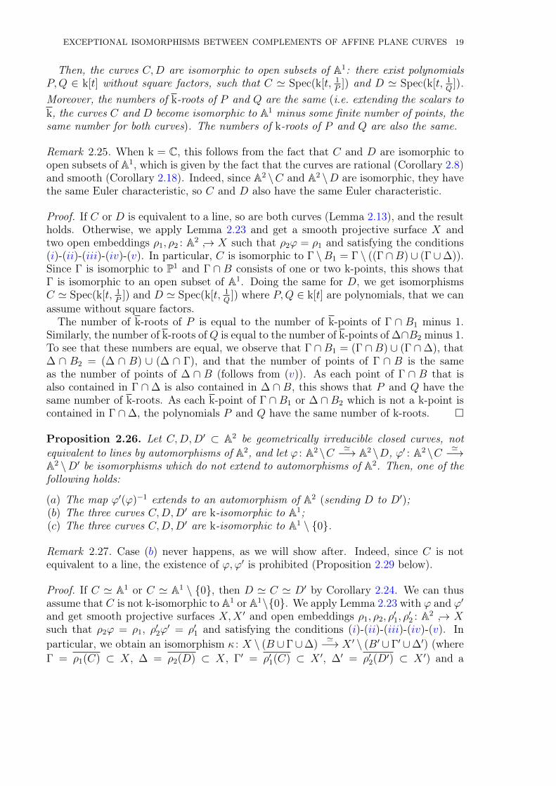
Proposition 2.26. Let C,D,D′ ⊂ A2 be geometrically irreducible closed curves, notequivalent to lines by automorphisms of A2, and let ϕ : A2\C '−→ A2\D, ϕ′ : A2\C '−→A2 \D′ be isomorphisms which do not extend to automorphisms of A2. Then, one of thefollowing holds:
(a) The map ϕ′(ϕ)−1 extends to an automorphism of A2 (sending D to D′);(b) The three curves C,D,D′ are k-isomorphic to A1;(c) The three curves C,D,D′ are k-isomorphic to A1 \ {0}.
Remark 2.27. Case (b) never happens, as we will show after. Indeed, since C is notequivalent to a line, the existence of ϕ, ϕ′ is prohibited (Proposition 2.29 below).
Proof. If C ' A1 or C ' A1 \ {0}, then D ' C ' D′ by Corollary 2.24. We can thusassume that C is not k-isomorphic to A1 or A1\{0}. We apply Lemma 2.23 with ϕ and ϕ′and get smooth projective surfaces X,X ′ and open embeddings ρ1, ρ2, ρ
′1, ρ′2 : A2 ↪→ X
such that ρ2ϕ = ρ1, ρ′2ϕ′ = ρ′1 and satisfying the conditions (i)-(ii)-(iii)-(iv)-(v). Inparticular, we obtain an isomorphism κ : X \ (B ∪Γ∪∆)
'−→ X ′ \ (B′ ∪Γ′ ∪∆′) (whereΓ = ρ1(C) ⊂ X, ∆ = ρ2(D) ⊂ X, Γ′ = ρ′1(C) ⊂ X ′, ∆′ = ρ′2(D′) ⊂ X ′) and a
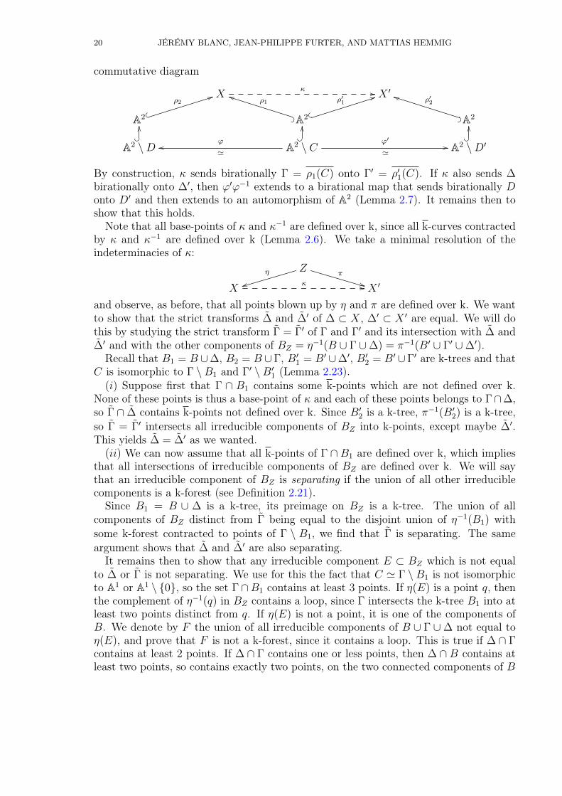
20 JÉRÉMY BLANC, JEAN-PHILIPPE FURTER, AND MATTIAS HEMMIG
commutative diagram
Xκ // X ′
A2 '�
ρ244
A2W7
ρ1jj
' �
ρ′144
A2W7
ρ′2jj
A2 \D?�
OO
A2 \ Cϕ
'oo ϕ′
'//
?�
OO
A2 \D′?�
OO
By construction, κ sends birationally Γ = ρ1(C) onto Γ′ = ρ′1(C). If κ also sends ∆birationally onto ∆′, then ϕ′ϕ−1 extends to a birational map that sends birationally Donto D′ and then extends to an automorphism of A2 (Lemma 2.7). It remains then toshow that this holds.
Note that all base-points of κ and κ−1 are defined over k, since all k-curves contractedby κ and κ−1 are defined over k (Lemma 2.6). We take a minimal resolution of theindeterminacies of κ:
Zη
ttπ
**Xκ // X ′
and observe, as before, that all points blown up by η and π are defined over k. We wantto show that the strict transforms ∆ and ∆′ of ∆ ⊂ X, ∆′ ⊂ X ′ are equal. We will dothis by studying the strict transform Γ = Γ′ of Γ and Γ′ and its intersection with ∆ and∆′ and with the other components of BZ = η−1(B ∪ Γ ∪∆) = π−1(B′ ∪ Γ′ ∪∆′).
Recall that B1 = B ∪∆, B2 = B ∪Γ, B′1 = B′ ∪∆′, B′2 = B′ ∪Γ′ are k-trees and thatC is isomorphic to Γ \B1 and Γ′ \B′1 (Lemma 2.23).
(i) Suppose first that Γ ∩ B1 contains some k-points which are not defined over k.None of these points is thus a base-point of κ and each of these points belongs to Γ∩∆,so Γ ∩ ∆ contains k-points not defined over k. Since B′2 is a k-tree, π−1(B′2) is a k-tree,so Γ = Γ′ intersects all irreducible components of BZ into k-points, except maybe ∆′.This yields ∆ = ∆′ as we wanted.
(ii) We can now assume that all k-points of Γ ∩ B1 are defined over k, which impliesthat all intersections of irreducible components of BZ are defined over k. We will saythat an irreducible component of BZ is separating if the union of all other irreduciblecomponents is a k-forest (see Definition 2.21).
Since B1 = B ∪ ∆ is a k-tree, its preimage on BZ is a k-tree. The union of allcomponents of BZ distinct from Γ being equal to the disjoint union of η−1(B1) withsome k-forest contracted to points of Γ \ B1, we find that Γ is separating. The sameargument shows that ∆ and ∆′ are also separating.
It remains then to show that any irreducible component E ⊂ BZ which is not equalto ∆ or Γ is not separating. We use for this the fact that C ' Γ \B1 is not isomorphicto A1 or A1 \ {0}, so the set Γ∩B1 contains at least 3 points. If η(E) is a point q, thenthe complement of η−1(q) in BZ contains a loop, since Γ intersects the k-tree B1 into atleast two points distinct from q. If η(E) is not a point, it is one of the components ofB. We denote by F the union of all irreducible components of B ∪ Γ ∪∆ not equal toη(E), and prove that F is not a k-forest, since it contains a loop. This is true if ∆ ∩ Γcontains at least 2 points. If ∆ ∩ Γ contains one or less points, then ∆ ∩ B contains atleast two points, so contains exactly two points, on the two connected components of B

EXCEPTIONAL ISOMORPHISMS BETWEEN COMPLEMENTS OF AFFINE PLANE CURVES 21
which both intersect Γ and ∆ (see Lemma 2.23(v)). We again get a loop on the unionof Γ, ∆ and of the connected component of B not containing η(E). The fact that Fcontains a loop implies that η−1(F ) contains a loop, and achieves to prove that E is notseparating. �
2.6. The case of curves isomorphic to A1 and the proof of Theorem 1. To finishthe proof of Theorem 1, one still needs to do the case of curves isomorphic to A1. Thecase of lines has already been treated in Lemma 2.13. In characteristic zero, this finishesthe study by the Abyhankar-Moh-Suzuki theorem, but in positive characteristic, thereare many closed curves of A2 which are isomorphic to A1 but are not equivalent to lines(these curves are sometimes called “bad lines” in the literature). We will show that anopen embedding A2 \ C ↪→ A2 always extends to A2 if C is isomorphic to A1 but notequivalent to a line.
Lemma 2.28. Let n ≥ 1 and let Γ ⊂ Fn be a geometrically irreducible closed curve,such that Γ · Fn ≥ 2. If there exists a birational map Fn 99K P2 that contracts Γ toa point (and maybe contracts some other curves), then Γ is geometrically rational andsingular. Moreover, one of the following occurs:(a) There exists a point p ∈ Fn(k) such that 2mp(Γ) > Γ · Fn.(b) We have n = 1 and there exists a point p ∈ F1(k) \ S1 such that mp(Γ) > Γ · S1.
Proof. We can assume that k = k. Denote by ψ : Fn 99K P2 the birational map thatcontracts C to a point (and maybe some other curves). The minimal resolution of thismap yields a commutative diagram
Xη
ttπ
**Fnϕ // P2
In Pic(Fn) = ZFn⊕
ZSn we write
Γ = aSn + bFn−KFn = 2Sn + (2 + n)Fn
for some integers a, b. Note that a = Γ · Fn ≥ 2 and that b − an = Γ · Sn ≥ 0. Byhypothesis, the strict transform Γ of Γ on X is a smooth curve contracted by π. Inparticular, Γ is rational and the divisor 2Γ + aKX is not effective, since
(2Γ + aKX) · π∗(L) = aKX · π∗(L) = aπ∗(KP2) · π∗(L) = aKP2 · L = −3a < 0
for a general line L ⊂ P2.Denoting by E1, . . . , Er ∈ Pic(X) the pull-backs of the exceptional divisors blown up
by η (which satisfy (Ei)2 = −1 for each i and Ei · Ej = 0 for i 6= j) we have
Γ = aη∗(Sn) + bη∗(Fn) −∑r
i=1miEi−KX = 2η∗(Sn) + (2 + n)η∗(Fn) −
∑ri=1Ei
2Γ + aKX = (2b− a(2 + n))η∗(Fn) +∑r
i=1(a− 2mi)Ei
which implies, since 2Γ + aKX is not effective, that either 2b < a(2 + n) or 2mi > a forsome i. If 2mi > a for some i, we get (a), since the mi are the multiplicities of Γ at thepoints blown up by η.

22 JÉRÉMY BLANC, JEAN-PHILIPPE FURTER, AND MATTIAS HEMMIG
It remains to study the case where 2mi ≤ a for each i, and where 2b < a(2 + n).Remembering that b− an = Γ · Sn ≥ 0, one finds n ≤ b
a< 2+n
2, whence n = 1 and thus
2b < 3a. We then compute
3Γ + bKX = (3a− 2b)η∗(Sn) +∑r
i=1(b− 3mi)Ei
which is again not effective, since (3Γ + bKX) · π∗(L) = bKX · π∗(L) = −3b < 0 for ageneral line L ⊂ P2, because b ≥ an = a ≥ 2. This implies that there exists an integer isuch that 3mi > b. Since 2mi ≤ a, one finds mi > b− a = Γ · S1, which yields (b). �
Proposition 2.29. Let C ⊂ A2 be a closed curve, isomorphic to A1 (i.e. isomorphic toA1 over k). The following are equivalent:(a) The curve C is equivalent to a line by an automorphism of A2.(b) There exists an open embedding A2 \C ↪→ A2 which does not extend to an automor-
phism of A2.(c) Embedding A2 into P2, via the canonical embedding, there exists a birational map
of P2 that contracts the curve C to a point (and maybe contracts other curves).
Proof. The implications (a)⇒ (b) and (a)⇒ (c) can be observed, for example by takingthe map (x, y) 7→ (x, xy), which is an open embedding of A2 \ {x = 0} into A2, whichdoes not extend to an automorphism of A2, and whose extension to P2 contracts the linex = 0 to a point.
To prove (b) ⇒ (c), we take an open embedding ϕ : A2 \ C ↪→ A2 which does notextend to an automorphism of A2 and look at the extension to P2. By Lemma 2.7,either this one contracts C, or C is equivalent to a line, in which case (c) is true as wasshown before.
It remains to prove (c) ⇒ (a). We apply Lemma 2.16, and obtain an isomorphismι : A2 '−→ Fn\(Sn ∪ Fn) such that the closure of ι(C) in Fn is a curve Γ which satisfiesone of the two cases (1)-(2) of Lemma 2.16. In case (1), the curve is equivalent to a lineas it is isomorphic to A1 (equivalence (ii) − (iii) of Lemma 2.16). It remains to studythe case where Γ satisfies the conditions (2) of Lemma 2.16 (in particular Γ · Fn ≥ 2),and to show that these, together with (c), yield a contradiction. We prove that there isno point p ∈ Fn(k) such that 2mp(Γ) > Γ ·Fn. Indeed, since Γ ·Fn ≥ 2, the point wouldbe a singular point of Γ, and since Γ \ (Sn ∪ Fn) = ι(C) ' C is isomorphic to A1, p is ak-point and is the unique k-point of Γ∩ (Sn ∪Fn). Moreover, as Γ ·Fn ≥ 2, we find thatp ∈ Fn. Since 2mp(Γ) > Γ ·Fn and because Γ satisfies the conditions (2) of Lemma 2.16,the only possibility is that n = 1, p ∈ F1 \S1 and 0 < mp(Γ) ≤ Γ ·S1. This is impossibleas it contradicts the fact that Γ ∩ (S1 ∪ F1) contains only one k-point.
Denote by ψ0 : P2 99K P2 the birational map that contracts C (and maybe othercurves) to a point. Observe that ψ0 ◦ ι−1 yields a birational map ψ : Fn 99K P2 whichcontracts Γ to a point. As there is no point p ∈ Fn(k) such that 2mp(Γ) > Γ · Fn,Lemma 2.28 implies that n = 1 and that there exists a point p ∈ F1(k) \ S1 such thatmp(Γ) > Γ · S1. Again, this point is a k-point, since C is k-isomorphic to A1. Thiscontradicts the conditions (2) of Lemma 2.16. �
Remark 2.30. If k is algebraically closed, the equivalence between conditions (a) and (c)of Proposition 2.29 can also be proven using Kodaira dimension. Let us introduce thefollowing conditions:

EXCEPTIONAL ISOMORPHISMS BETWEEN COMPLEMENTS OF AFFINE PLANE CURVES 23
(a)′ The Kodaira dimension κ(C,A2) of C is equal to −∞.(c)′ There exists a birational transformation of P2 sending C onto a line.
The equivalence between (a) and (a)′ follows from [Gan85, Theorem 2.4.(1)] and theequivalence between (a)′ and (c)′ is Coolidge’s theorem (see e.g. [KM83, Theorem 2.6]).Let us now recall how the classical equivalence between (c) and (c)′ can be proven. Everysimple quadratic birational transformation of P2 contracts three lines and no other curve.This yields (c)′ ⇒ (c). To get (c) ⇒ (c)′, we take a birational transformation ϕ of P2
that contracts C to a point and decompose ϕ as ϕ = ϕr ◦ · · · ◦ ϕ1, where each ϕi isa simple quadratic transformation (using Castelnuovo-Noether factorisation theorem).Choosing i ≥ 1 as the smallest integer such that (ϕi ◦ · · · ◦ ϕ1)(C) is a point, the curve(ϕi−1 ◦ · · · ◦ ϕ1)(C) is contracted by ϕi and is thus a line.
Remark 2.31. If the field k is perfect, then every curve that is geometrically isomorphic toA1 (i.e. over k) is also isomorphic to A1. This can be seen by embedding the curve in P1
and looking at the complement point, necessarily defined over k. For non-perfect fields,there exist closed curves C ⊂ A2 geometrically isomorphic to A1 but not isomorphic toA1 (see [Rus70]). Corollary 2.24 shows that every open embedding A2 \C ↪→ A2 extendsto an automorphism of A2 for all such curves.
We can now finish the section by proving Theorem 1:
Proof of Theorem 1. We recall the hypothesis of the theorem: we have a geometricallyirreducible closed curve C ⊂ A2 and an isomorphism ϕ : A2 \ C '−→ A2 \ D for someclosed curve C ⊂ A2. Assume that ϕ does not extend to an automorphism of A2.
(1): If C is isomorphic to A1, then the implication (b)⇒ (a) of Proposition 2.29 showsthat C is equivalent to a line and Lemma 2.13(2) implies that the same holds for D. Inparticular, the curves C and D are isomorphic.
If C is isomorphic to A1 \ {0} then so is D by Corollary 2.24.(2): if C is not isomorphic to A1 or to A1 \ {0}, then Proposition 2.26 shows that the
isomorphism ϕ : A2\C '−→ A2\D (not extending to an automorphism of A2) is uniquelydetermined by C, up to left composition by an automorphism of A2. In particular, thereare at most two equivalence classes of curves of A2 having complements isomorphicto A2 \ C. Corollary 2.24 achieves the proof by giving the existence of isomorphismsC ' Spec(k[t, 1
P]) and D ' Spec(k[t, 1
Q]) for some square-free polynomials P,Q ∈ k[t]
that have the same number of roots in k, and also the same number of roots in thealgebraic closure of k. �
3. Families of non-equivalent embeddings
As we observed in Lemma 2.16 and its applications, the curves of A2 given by
a(y)x+ b(y) = 0
for some coprime polynomials a, b ∈ k[y], a 6= 0 (where we can always assume thatdeg b < deg a), yield a natural family which plays an important role. We study thisfamily here. Recall that such curves are isomorphic to a line if and only a(y) is aconstant (Lemma 2.16(i)-(iii)). Actually, we have the following obvious and strongerresult:

24 JÉRÉMY BLANC, JEAN-PHILIPPE FURTER, AND MATTIAS HEMMIG
Lemma 3.1. Let C ⊂ A2 be the irreducible curve given by the equation
a(y)x+ b(y) = 0,
where a, b ∈ k[y] are coprime polynomials and a is nonzero. Then, the algebra of regularfunctions on C is isomorphic to k[y, 1/a(y)].
Proof. The algebra of regular functions on C satisfies
k[C] = k[x, y]/(a(y)x+ b(y)) ' k[y,−b(y)/a(y)] = k[y, 1/a(y)],
where the last equality comes from the fact that there exist c, d ∈ k[y] with ad− bc = 1,which implies that 1
a= ad−bc
a= d− c · b
a∈ k[y, b
a]. �
3.1. A construction using elements of SL2(k[y]).
Lemma 3.2. For each matrix(a(y) b(y)c(y) d(y)
)∈ SL2(k[y]), we have an isomorphism
ϕ : A2 \ C '−→ A2 \D(x, y) 7→
( c(y)x+d(y)a(y)x+b(y)
, y)
where C,D ⊂ A2 are given by a(y)x+ b(y) = 0 and a(y)x− c(y) = 0 respectively.
Proof. Note first that ϕ is a birational transformation of A2, with inverse ψ : (x, y) 7→(−b(y)x+d(y)a(y)x−c(y)
, y). It remains to prove that the isomorphism ϕ∗ : k(x, y) → k(x, y), x 7→cx+dax+b
, y 7→ y induces an isomorphism k[x, y, 1ax−c ] → k[x, y, 1
ax+b]. This follows from the
equalities:ϕ∗(x) = cx+d
ax+b, ϕ∗(y) = y, ϕ∗
(1
ax−c
)= ax+ b and
ψ∗(x) = −bx+dax−c , ψ∗(y) = y, ψ∗
(1
ax+b
)= ax− c. �
The curves C and D of Lemma 3.2 are always isomorphic thanks to Lemma 3.1. Wenow prove that they are in general not equivalent.
Lemma 3.3. Let C1, C2 ⊂ A2 be two irreducible curves given by
a1(y)x+ b1(y) = 0 and a2(y)x+ b2(y) = 0
respectively, for some polynomials a1, a2, b1, b2 ∈ k[y] such that deg a1 > deg b1 ≥ 0 anddeg a2 > deg b2 ≥ 0. Then, the curves C1 and C2 are equivalent if and only if there existconstants α, λ, µ ∈ k∗ and β ∈ k such that
a2(y) = λ · a1(αy + β), b2(y) = µ · b1(αy + β).
Proof. We first observe that if a2(y) = λ · a1(αy + β) and b2(y) = µ · b1(αy + β) forsome α, λ, µ ∈ k∗, β ∈ k, then the automorphism (x, y) 7→ (λ
µx, αy + β) of A2 sends C2
onto C1.Conversely, we assume the existence of ϕ ∈ Aut(A2) that sends C2 onto C1 and want
to find α, λ, µ ∈ k∗, β ∈ k as above. Writing ϕ as (x, y) 7→ (f(x, y), g(x, y)) for somepolynomials f, g ∈ k[x, y], one gets
(A) µ(a1(g)f + b1(g)
)= a2(y)x+ b2(y)
for some µ ∈ k∗.
EXCEPTIONAL ISOMORPHISMS BETWEEN COMPLEMENTS OF AFFINE PLANE CURVES 25
(i) If g ∈ k[y], the fact that k[f, g] = k[x, y] implies that g = αy+β, f = γx+ s(y) forsome α, γ ∈ k∗, β ∈ k and s(y) ∈ k[y]. This yields a1(g)f + b1(g) = a1(g)(γx + s(y)) +b1(g), so that Equation (A) gives:
a2 = µγ · a1(g), b2 = µ ·(a1(g)s(y) + b1(g)
).
This shows in particular that deg a1 = deg a2, whence deg b2 < deg a1(g). Since deg b1(g) <deg a1(g), we find that s = 0, and thus that b2 = µ · b1(g), as desired. This ends theproof, by choosing λ = µγ.
(ii) It remains to study the case where g /∈ k[y], which corresponds to degx(g) ≥ 1.This yields degx a1(g) = deg a1 · degx(g) > deg b1 · degx(g) = degx b1(g), which impliesthat degx
(a1(g)f + b1(g)
)= deg(a1) · degx(g) + degx(f). Equation (A) shows that this
degree is 1, and since deg a1 ≥ 1, we find deg a1 = 1. Similarly, the automorphismsending C1 onto C2 satisfies the same condition, so deg a2 = 1. This implies thatb1, b2 ∈ k∗. There exist thus some α, λ, µ ∈ k∗, β ∈ k such that a2(y) = λ · a1(αy + β)and b2(y) = µ · b1(αy + β). �
Corollary 3.4. For each polynomial f ∈ k[t] of degree ≥ 1, there exist two closed curvesC,D ⊂ A2, both isomorphic to Spec(k[t, 1
f]), that are non-equivalent and have isomorphic
complements. Moreover, the set of all such pairs (C,D), up to equivalence, is infinite.
Proof. We choose an irreducible polynomial b ∈ k[t] which does not divide f . For eachn ≥ 1 such that deg(fn) > 2 deg(b), we then choose two polynomials c, d ∈ k[t] suchthat fnd− bc = 1 (possible since gcd(fn, b) = 1). Replacing c, d with c+αfn, d+αb, wecan moreover assume that deg c < deg fn. The curves Cn, Dn ⊂ A2 given by f(y)nx +b(y) = 0 and f(y)nx − c(y) = 0 are both isomorphic to Spec(k[t, 1
fn]) = Spec(k[t, 1
f])
by Lemma 3.1 and have isomorphic complements by Lemma 3.2. Moreover, as deg bc =deg(fnd−1) ≥ deg(fn) > 2 deg(b), we find that deg c > deg b, which implies that Cn andDn are not equivalent by Lemma 3.3. Moreover, the curves Cn are all non-equivalent,again by Lemma 3.3. �
3.2. Curves isomorphic to A1 \ {0}. We consider now families of curves of A2 of theform xyd + b(y) = 0 for some d ≥ 1 and some polynomial b(y) ∈ k[y] satisfying b(0) 6= 0.Note that all these curves are isomorphic to Spec(k[y, 1
yd]) = Spec(k[y, 1
y]) ' A1 \ {0} by
Lemma 3.1.
Lemma 3.5. Let d ≥ 1 be an integer and b(y) ∈ k[y] be a polynomial satisfying b(0) 6= 0.We define Db ⊂ A2 to be the curve given by the equation
xyd + b(y) = 0
and ϕb to be the birational endomorphism of A2 given by
ϕb(x, y) = (xyd + b(y), y).
Denote by Lx, resp. Ly, the line of A2 given by the equation x = 0, resp. y = 0.(1) The transformation ϕb induces an automorphism of A2 \ Ly and an isomorphism
A2 \ (Ly ∪Db)'−→ A2 \ (Ly ∪ Lx).

26 JÉRÉMY BLANC, JEAN-PHILIPPE FURTER, AND MATTIAS HEMMIG
(2) Assume now that b has degree ≤ d− 1 and fix an integer m ≥ 1. Then, there existsa unique polynomial c ∈ k[y] of degree ≤ d− 1 satisfying
(B) b(y) ≡ c(yb(y)m) (mod yd).
Furthermore, we have c(0) 6= 0.(3) Define the birational transformations τ and ψb,m of A2 by
τ(x, y) = (x, xy) and ψb,m = (ϕc)−1τmϕb.
Then, ψb,m induces an isomorphism A2 \Db'−→ A2 \Dc whose expression is
ψb,m = (x, y) =
x+ λ+ yf(x, y)(xyd + b(y)
)md , y (xyd + b(y))m ,
for some constant λ ∈ k and some polynomial f ∈ k[x, y] (depending on b and m).(4) Fixing the polynomial b, all open embeddings A2 \ Db ↪→ A2 given by ψb,m, m ≥ 1,
are different, up to left composition by automorphisms of A2.
Proof. (1): The automorphism (ϕb)∗ of k(x, y) satisfies
(ϕb)∗(x) = xyd + b(y) and (ϕb)
∗(y) = y.
The result follows from the two following equalities:(ϕb)
∗(k[x, y, 1y]) = k[xyd + b(y), y, 1
y] = k[x, y, 1
y] and
(ϕb)∗(k[x, y, 1
x, 1y]) = k[xyd + b(y), 1
xyd+b(y), y, 1
y] = k[x, y, 1
y, 1xyd+b(y)
].
(2): Since b(0) 6= 0, the endomorphism of the algebra k[y]/(yd) defined by y 7→ yb(y)m
is an automorphism. If the inverse automorphism is given by y 7→ u(y), note that (B)is equivalent to c(y) ≡ b(u(y)) (mod yd). This determines uniquely the polynomial c.Finally, replacing x by zero in (B), we get c(0) = b(0) 6= 0.
(3): Since τ induces an automorphism of A2 \ (Ly ∪ Lx), assertion (1) implies that ψinduces an isomorphism A2 \ (Ly ∪Db)
'−→ A2 \ (Ly ∪Dc) (this would be true for anychoice of c). It remains to see that the choice of c that we have made implies that ψextends to an isomorphism A2 \Db
'−→ A2 \Dc of the desired form.Since (ϕc)
−1(x, y) =(x−c(y)yd
, y), τm(x, y) = (x, xmy) and ψb,m = (ϕc)
−1τmϕb, we get:
(C)ψb,m(x, y) = (ϕc)
−1τm(xyd + b(y), y)
=(xyd+b(y)−c(y∆)
yd∆d , y∆), with ∆ = (xyd + b(y))m.
To show that ψb,m has the desired form, we use b(y) ≡ c(yb(y)m) (mod yd) (Equation(B)), which yields λ ∈ k such that b(y) ≡ c(yb(y)m) + λyd (mod yd+1). Since y∆ ≡yb(y)m (mod yd+1), we get b(y) ≡ c(y∆) + λyd (mod yd+1). There is thus f ∈ k[x, y]such that
xyd + b(y)− c(y∆) = yd(x+ λ+ yf(x, y)).
This yields the desired form for ψb,m and shows that ψb,m restricts to the automorphismx 7→ x+ λ on Ly and then restricts to an isomorphism A2 \Db
'−→ A2 \Dc.(4): It is enough to check that for m > n ≥ 1 the birational transformation θ =
ψb,n◦(ψb,m)−1 of A2 does not correspond to an automorphism of A2. Setting l = m−n ≥ 1

EXCEPTIONAL ISOMORPHISMS BETWEEN COMPLEMENTS OF AFFINE PLANE CURVES 27
and denoting by cm and cn the elements of k[y] associated to b and to the integers mand n respectively, we get
θ =((ϕcn)−1τnϕb
)◦(
(ϕcm)−1τmϕb
)−1
= (ϕcn)−1τ−lϕcm .
The second component of θ(x, y) is thus equal to the second component of τ−lϕcm(x, y)which is y
(xyd+cm(y))l∈ k(x, y) \ k[x, y]. This shows that θ is not an automorphism of A2
(and even not an endomorphism) and achieves the proof. �
Remark 3.6. Note that Lemma 3.5(1) provides us an isomorphism A2 \ (Ly ∪ Db)'−→
A2 \ (Ly ∪ Lx) where the reducible curves (Ly ∪Db) and (Ly ∪ Lx) are not isomorphic.Indeed, the reducible curve (Ly∪Db) has two connected components (since Ly∩Db = ∅),while the reducible curve (Ly∪Lx) is connected (since Ly∩Lx 6= ∅). As noted in [Kra96],this kind of easy examples explains why the complement problem in An has only beenformulated for irreducible hypersurfaces.
Remark 3.7. Geometrically, the construction of Lemma 3.5(3) can be interpreted asfollows: the birational morphism ϕb : (x, y) 7→ (xyd + b(y), y) contracts the line y = 0to the point (b(0), 0). If d = 1 then ϕb just sends the line onto the exceptional divisorof (b(0), 0). If d ≥ 2, it sends the line onto the exceptional divisor of a point in the(d−1)-th neighbourhood of (b(0), 0). The coordinates of these points are determined bythe polynomial b. The fact that τm : (x, y) 7→ (x, xmy) contracts the line x = 0 impliesthat ψb,m contracts the curve Db given by xyd + b(y) = 0. Moreover, τm fixes the point(b(0), 0) and induces a local isomorphism around it, so acts on the set of infinitely nearpoints. This action changes the polynomial b and replaces it with another one, which isthe polynomial c = cb,m provided by Lemma 3.5(2).
Corollary 3.8. For each field k, there exists an infinite sequence of curves Ci ⊂ A2,i ∈ N, all pairwise non-equivalent under automorphisms, all isomorphic to A1 \ {0} andsuch that for each i there are infinitely many open embeddings A2 \ Ci ↪→ A2, up toautomorphisms of A2.
Proof. It suffices to choose the curve Ci given by xyi+2 + y + 1, for each i ≥ 2. Thesecurves are all isomorphic to A1\{0} by Lemma 3.1 and are pairwise non-equivalent, underautomorphisms of A2, by Lemma 3.3. The existence of infinitely many open embeddingsA2 \ Ci ↪→ A2, up to automorphisms of A2, is then ensured by Lemma 3.5(4). �
One can compute the polynomial c = cb,m provided by Lemma 3.5(2), in terms of band m, and find explicit formulas. We find in particular the following result:
Lemma 3.9. For each µ ∈ k define the curve Cµ ⊂ A2 by
xy3 + µy2 + y + 1 = 0.
Then, there exists an isomorphism A2 \Cµ'−→ A2 \Cµ−1. In particular, if char(k) = 0,
we obtain infinitely many closed curves of A2, not equivalent under automorphisms ofA2, which have isomorphic complements.
Proof. The isomorphism between A2 \Cµ and A2 \Cµ−1 follows from Lemma 3.5 appliedwith d = 3, m = 1, b = µy2 + y + 1 and c = (µ− 1)y2 + y + 1.

28 JÉRÉMY BLANC, JEAN-PHILIPPE FURTER, AND MATTIAS HEMMIG
To get the last statement, one assumes that char(k) = 0 and observes that the affinesurfaces A2 \ Cn are all isomorphic for each n ∈ Z. To show that the curves Cn, n ∈ Zare pairwise non-equivalent, we apply Lemma 3.3: for m,n ∈ Z, the curves Cm and Cnare equivalent only if there exist α, λ, µ ∈ k∗, β ∈ k such that
y3 = λ · (αy + β)3, my2 + y + 1 = µ ·(n(αy + β)2 + (αy + β) + 1
).
The first equality yields β = 0, which yields, together with the second equation my2 +y + 1 = µ · (nα2y2 + αy + 1), so µ = 1, α = 1 and thus m = n, as we wanted. �
If char(k) = p > 0, Lemma 3.9 only gives p non-equivalent curves that have isomorphiccomplements. We can get more curves by applying Lemma 3.3 to polynomials of higherdegree:
Lemma 3.10. For each integer n ≥ 1 there exist curves C1, . . . , Cn ⊂ A2, all isomorphicto A1 \ {0}, pairwise non-equivalent, such that all surfaces A2 \ C1, . . . , A2 \ Cn areisomorphic.
Proof. The case where char(k) = 0 is provided by Lemma 3.9 so we can assume thatchar(k) = p ≥ 2. Set b(y) = 1+y and d = pn+2. For each integer i satisfying 1 ≤ i ≤ n,we apply Lemma 3.5(2) with m = pi. Hence, there exists a unique polynomial ci ∈ k[y]of degree ≤ d− 1 satisfying
(D) b(y) ≡ ci(yb(y)pi
) (mod yd).
Define Ci ⊂ A2 to be the curve given by the equation
xyd + ci(y) = 0.
By Lemma 3.5(3), all surfaces A2 \ C1, . . . , A2 \ Cn are isomorphic to A2 \ D, whereD ⊂ A2 is given by
xyd + b(y) = 0.
It remains to check that C1, . . . , Cn are pairwise non-equivalent. Assume therefore thatCi and Cj are equivalent. By Lemma 3.3, there exist α, λ, µ ∈ k∗, β ∈ k such that
yd = λ · (αy + β)d, cj(y) = µ · ci(αy + β).
The first equality yields β = 0, so that we get:
(E) cj(y) = µ · ci(αy).
However, by Equation (D) we have
1 + y ≡ ci(y + ypi+1) (mod yp
i+2)
and this equation admits the unique solution
ci = 1 + y − ypi+1 + (terms of higher order).
(The unicity follows for example again from Lemma 3.5(2)). Hence, looking at theequation (E) modulo y2, we obtain 1 + y = µ(1 + αy), so that we get α = µ = 1.Equation (E) finally yields ci = cj, so that the above (partial) computation of ci givesus i = j. �
The proof of Theorem 2 is now finished:

EXCEPTIONAL ISOMORPHISMS BETWEEN COMPLEMENTS OF AFFINE PLANE CURVES 29
Proof of Theorem 2. Part (1) corresponds to Corollary 3.8. Part (2) is given by Corol-lary 3.9 (char(k) = 0) and Lemma 3.10 (char(k) > 0). Part (3) corresponds to Corol-lary 3.4. �
4. Non-isomorphic curves with isomorphic complements
4.1. A geometric construction. We begin with the following fundamental construc-tion:
Lemma 4.1. Let d ≥ 3 be an integer. Let Γ ⊂ P2 be the cuspidal rational curve ofequation
yd−1z = Pd(x, y),
where Pd is a homogeneous polynomial of degree d which is not a multiple of y. Notethat the point q1 = [0 : 0 : 1] ∈ P2(k) has multiplicity d− 1 on Γ and that it is thereforethe unique singular point of this curve (this comes for example from the genus formulaof a plane curve). Let ∆, L be two lines of P2 such that L ∩ Γ = {p1, q1} for some pointp1 ∈ P2(k) \ {q1}, and assume that ∆ does not pass through p1 nor q1.
Γ
L
∆
q1
p1
Denote by π : X → P2 the birational morphism given by the blow-up of p1, q1, fol-lowed by the blow-up of the points p2,. . . ,pd−1 and q2,. . . ,qd infinitely near p1 and q1
respectively and all belonging to the strict transform of Γ. Denote by Γ, ∆, L, E1,. . . ,Ed−1, F1,. . . ,Fd ⊂ X the strict transforms of Γ, ∆, L and of the exceptional divisorsabove p1,. . . ,pd−1, q1, . . . ,qd. Consider the tree (which is even a chain)
B = L ∪d−2⋃i=1
Ei ∪d⋃i=1
Fi.
Then, the two surfaces X \(Γ∪B) and X \(∆∪B) are both isomorphic to A2. Moreover,the situation on X is depicted on the symmetric diagram (F),
(F)
−d−1−2 −1 −2 −2 −2−2−2 . . . . . .−1 −1
∆ Γ1 1E1Ed−3Ed−1 Ed−2 L
F1
Fd Fd−1 F3 RF2
where all curves are isomorphic to P1, all intersections indicated are transversal in ex-actly one k-point, except for Γ∩∆, which can be more complicated (the picture just shows

30 JÉRÉMY BLANC, JEAN-PHILIPPE FURTER, AND MATTIAS HEMMIG
the case where we get 3 points with transversal intersection), and where the numbers in-dicated are the self-intersections. The curve R is the strict transform of the line R ofequation y = 0 (tangent to Γ at q1).
In particular, this construction provides an isomorphism A2 \ C ' A2 \ D, whereC,D ⊂ A2 are closed curves isomorphic to Γ\(B∪∆) ' Γ\(∆∪{q1}) and ∆\(B∪ Γ) '∆ \ (Γ∪L) respectively, both of degree d2− d+ 1. Moreover, the closure C of C ⊂ A2 inP2 admits exactly two singular points, which lie on the line at infinity. The sequences ofmultiplicities of these two singular points are (d, . . . , d︸ ︷︷ ︸
d−1
) and ((d− 1)2, d− 1, . . . , d− 1︸ ︷︷ ︸d
).
Proof. Blowing up once the singular point q1 of Γ, the strict transform of Γ becomes asmooth rational curve having (d− 1)-th order contact with the exceptional divisor. Theunique point of intersection between the strict transform and the exceptional divisorcorresponds to the direction of the tangent line R. Hence, all points q2, . . . , qd belong tothe strict transform of the exceptional divisor of q1. This gives the self-intersections ofF1, . . . , Fd and their configurations, as shown on diagram (F). As p1 is a smooth pointof Γ, the curves E1, . . . , Ed−1 form a chain of curves, as shown on diagram (F). The restof the diagram is checked by looking at the definitions of the curves Γ, ∆, L, R.
We want to show the existence of isomorphisms
ψ1 : X \ (B ∪ ∆)'−→ A2 and ψ2 : X \ (B ∪ Γ)
'−→ A2
such that C = ψ1(Γ\ (B∪ ∆)) and D = ψ2(∆\ (B∪ Γ)) are of degree d2−d+1. Indeed,the existence of ψ1, ψ2 implies that A2 \ C and A2 \D are isomorphic, and that C andD are isomorphic to Γ \ (B ∪ ∆) and ∆ \ (B ∪ Γ) respectively. The morphism π givesthen isomorphisms of these curves with Γ \ (∆ ∪ {q}) and ∆ \ (Γ ∪ L) respectively.
We first show that ψ1 exists. We observe that since π is the blow-up of 2d− 1 pointswhich are defined over k, the Picard group ofX is of rank 2d, over k and over its algebraicclosure k. We contract the curves Fd, . . . , F1 and obtain a smooth projective surfaceY of Picard rank d (again over k and k). The configuration of the image of the curvesE1, . . . , Ed−1, L, Γ is then depicted on diagram (G) (we omit to write the curve R as wewill not need it):
(G)
0L
−2E1
−2Ed−3
−1Ed−1
−2Ed−2
. . .1∆
d2 − d+ 1
Γ
In fact, Y is just the blow-up of the points p1, . . . , pd−1 starting from P2.In order to show that X \ (B ∪ ∆) ' Y \ (∆ ∪ L ∪ E1 ∪ · · · ∪ Ed−2) is isomorphic to
A2, we will construct a birational map ψ1 : Y 99K P2 which restricts to an isomorphismY \ (∆ ∪ L ∪ E1 ∪ · · · ∪ Ed−2)
'−→ P2 \ L for some line L. Let us now describe thismap. Denote by r1 the unique point of Y such that {r1} = ∆ ∩ L in Y . We blow up r1
and then the point r2 lying on the intersection of the exceptional curve of r1 and of thestrict transform of ∆. For i = 3, . . . , d, denoting by ri the point lying on the intersectionof the exceptional curve of ri−1 and on the strict transform of the exceptional curve ofr1, we successively blow up ri. We obtain thus a birational morphism θ : Z → Y . The

EXCEPTIONAL ISOMORPHISMS BETWEEN COMPLEMENTS OF AFFINE PLANE CURVES 31
configuration of curves on Z is depicted on diagram (H) (we again use the same name fora curve on Y and its strict transform on Z, and denote by Gi ⊂ Z the strict transformof the exceptional divisor of ri):
(H)
−1Gd
−2Gd−2
−2Gd−1
−1∆
−2G2
. . .
−1L
−dG1
−2E2
−2E1
−1Ed−1
−2Ed−2
. . .d2 − d+ 1
Γ
We can then contract the curves ∆,G2, . . . ,Gd−1, L, E1, . . . , Ed−2,G1 and obtain a bira-tional morphism ρ : Z → P2: The image of the target is P2 because it has Picard rank 1;note also that the image L of Gd is actually a line of P2 since it has self-intersection 1.The birational map ψ1 : Y 99K P2 given by ψ1 = ρθ−1 is the desired birational map. Theclosure C of C ⊂ A2 in P2 is then equal to the image of Γ by ρ.
For each contracted curve above, the multiplicity (on C) at the point where it iscontracted, is equal to d for ∆,G2, . . . ,Gd−1, it is equal to d − 1 for L, E1, . . . , Ed−2 andit is equal to (d − 1)2 for G1. Adding the singular point of multiplicity d − 1 of Γ, weobtain the two sequences of multiplicities (d, . . . , d︸ ︷︷ ︸
d−1
) and ((d− 1)2, d− 1, . . . , d− 1︸ ︷︷ ︸d
).
The self-intersection of C is then(d2 − d+ 1) + (d− 1) · d2 + (d− 1) · (d− 1)2 + ((d− 1)2)2 = (d2 − d+ 1)2,
which implies that the curve has degree d2 − d+ 1.The case of ψ2 is similar, as the diagram (F) is symmetric. �
Proposition 4.2. For each polynomial P ∈ k[t] of degree d ≥ 3 and each λ ∈ k withP (λ) 6= 0, there exist two closed curves C,D ⊂ A2 of degree d2 − d+ 1 such that A2 \Cand A2 \D are isomorphic and such that the following isomorphisms hold:
C ' Spec(
k[t,1
P])and D ' Spec
(k[t,
1
Q]), where Q(t) = P
(λ+
1
t
)· td.
Proof. Write Pd(x, y) = P (xy)yd ∈ k[x, y], which is a homogeneous polynomial of degree
d, such that Pd(x, 1) = P (x). Let then Γ,∆, L ⊂ P2 be the curves given by the equations
Γ : yd−1z = Pd(x, y), ∆ : z = 0, L : x = λy.
By construction, Pd is not divisible by y. Moreover, the two lines L and ∆ satisfyL ∩ Γ = {p1, q1} where p1 = [λ : 1 : P (λ)], q1 = [0 : 0 : 1] and ∆ does not pass throughp1 nor q1.
We apply Lemma 4.1, and obtain an isomorphism A2 \C ' A2 \D, where C,D ⊂ A2
are closed curves isomorphic to Γ\ (∆∪{q1}) and ∆\ (Γ∪L) respectively. Furthermore,both curves have degree d2 − d+ 1.
Since Γ \ {q1} is isomorphic to A1 via t 7→ [t : 1 : Pd(t, 1)] = [t : 1 : P (t)], we obtainthat C ' Γ \ (∆ ∪ {q1}) is isomorphic to Spec(k[t, 1
P]).
We then take the isomorphism A1 → ∆\L = ∆\{[λ : 1 : 0]} given by t 7→ [λt+1 : t : 0].The pull-back of ∆∩Γ corresponds to the zeroes of Pd(λt+1, t) = tdPd(λ+ 1
t, 1) = Q(t).
Hence, D is isomorphic to Spec(k[t, 1Q
]) as desired. �

32 JÉRÉMY BLANC, JEAN-PHILIPPE FURTER, AND MATTIAS HEMMIG
Corollary 4.3. For each d ≥ 0 and each distinct points a1, . . . , ad, b1, b2 ∈ P1(k), thereare two closed curves C,D ⊂ A2 such that A2 \ C and A2 \D are isomorphic and suchthat C ' P1 \ {a1, . . . , ad, b1} and D ' P1 \ {a1, . . . , ad, b2}.
Proof. The case where d ≤ 2 is obvious: Since PGL2(k) acts 3-transitively on P1(k),one can take C = D given by the equation x = 0, resp. xy = 1, resp. x(x − 1)y = 1,if d = 0, resp. d = 1, resp. d = 2. Let us now assume that d ≥ 3. Since PGL2(k)acts transitively on P1(k), we may assume without restriction that b1 is the point atinfinity [1 : 0]. Therefore, there exist distinct constants µ1, . . . , µd, λ ∈ k such thata1 = [µ1 : 1], . . . , ad = [µd : 1] and b2 = [λ : 1]. We now apply Proposition 4.2 withP =
∏di=1(t−µi). We get two closed curves C,D ⊂ A2 such that A2 \C and A2 \D are
isomorphic and such that C ' Spec(k[t, 1P
]) ' A1 \ {µ1, . . . , µd} ' P1 \ {a1, . . . , ad, b1}and D ' Spec(k[t, 1
Q]) ' A1 \ { 1
µ1−λ , . . . ,1
µd−λ}, where Q(t) = P (λ + 1
t) · td. It remains
to see that D is isomorphic to P1 \ {[µ1 : 1], . . . , [µd : 1], [λ : 1]} via t 7→ [λt+ 1 : t]. �
Corollary 4.4. If k is infinite and P ∈ k[t] is a polynomial with at least 3 roots in k,we can find two curves C,D ⊂ A2 that have isomorphic complements, such that C isisomorphic to Spec(k[t, 1
P]) but not D.
Proof. By Lemma 4.5 below, there exists a constant λ in k such that P (λ) 6= 0 andsuch that the curves Spec(k[t, 1
P]) and Spec(k[t, 1
Q]) are not isomorphic. The result now
follows from Proposition 4.2. �
Lemma 4.5. If k is infinite and P ∈ k[t] is a polynomial with at least 3 roots in k,then for a general λ ∈ k, the polynomial Q(t) = P (λ+ 1
t) · tdeg(P ) is such that the curves
Spec(k[t, 1P
]) and Spec(k[t, 1Q
]) are not isomorphic.
Proof. Let λ1, . . . , λd ∈ k be the single roots of P . It is enough to check that for a generalλ, there exists no automorphism of P1 sending {λ1, . . . , λd,∞} to { 1
λ1−λ , . . . ,1
λd−λ,∞}, or
equivalently that there exists no automorphism sending {λ1, . . . , λd,∞} to {λ1, . . . , λd, λ}.But, if an automorphism sends {λ1, . . . , λd,∞} to {λ1, . . . , λd, λ}, it necessarily belongsto the set A of automorphisms ϕ such that ϕ−1({λ1, λ2, λ3}) ⊂ {λ1, . . . , λd,∞}. Anautomorphism of P1 being determined by the image of 3 points, the set A has at most6(d+1
3
)= (d+ 1)d(d− 1) elements. As a conclusion, if λ is not of the form ϕ(µ) for some
ϕ ∈ A and some µ ∈ {λ1, . . . , λd,∞}, then no automorphism of P1 sends {λ1, . . . , λd,∞}to {λ1, . . . , λd, λ}. �
Remark 4.6. If k is a finite field (with at least 3 elements), then the conclusion ofCorollary 4.4 is false for the polynomial P =
∏α∈k
(x − α). Indeed, if C,D ⊂ A2 are two
curves such that C is isomorphic to Spec(k[t, 1P
]) and A2\C is isomorphic to A2\D, thenD is isomorphic to Spec(k[t, 1
Q]) for some polynomial Q without square factors having
the same number of roots in k and in k as P (Theorem 1(2)). This implies that Q isequal to µP for some µ ∈ k∗ and thus that C and D are isomorphic.
A similar argument holds for P =∏α∈k∗
(x−α) and P =∏
α∈k\{0,1}(x−α) (when the field
has at least 4, respectively 5 elements) since PGL2(k) acts 3-transitively on P1(k).

EXCEPTIONAL ISOMORPHISMS BETWEEN COMPLEMENTS OF AFFINE PLANE CURVES 33
Corollary 4.7. For each ground field k having more than 27 elements, one gets twogeometrically irreducible curves C,D ⊂ A2 of degree 7 which are not isomorphic butsuch that A2 \ C and A2 \D are isomorphic.
Proof. We fix some element ζ ∈ k \ {0, 1}. For each λ ∈ k \ {0, 1, ζ}, one can applyCorollary 4.3 with d = 3, a1 = [0 : 1], a2 = [1 : 1], a3 = [ζ : 1], b1 = [1 : 0],b2 = [λ : 1] and get two closed curves C,D ⊂ A2 such that A2 \ C and A2 \ D areisomorphic and such that C ' A1 \ {0, 1, ζ} = P1 \ {[0 : 1], [1 : 1], [ζ : 1], [1 : 0]} andD ' P1 \ {[0 : 1], [1 : 1], [ζ : 1], [λ : 1]}. It remains to see that one can find at least one λsuch that C and D are not isomorphic. Note that C and D are isomorphic if and onlyif there is an element of Aut(P1) = PGL2(k) that sends {[0 : 1], [1 : 1], [ζ : 1], [λ : 1]}onto {[0 : 1], [1 : 1], [ζ : 1], [1 : 0]}. The image of this element is determined by the imageof [0 : 1], [1 : 1], [ζ : 1], so one gets at most 24 automorphisms to avoid, hence at most24 elements of k \ {0, 1, ζ} to avoid. The field k having at least 28 elements, we find atleast one λ having the right property. �
We can now give the proof of Theorem 3.
Proof of Theorem 3. If the field is infinite (or simply has more than 27 elements), itfollows from Corollary 4.7. Let us therefore assume that k is a finite field. We againapply Proposition 4.2 (with λ = 0). Therefore, if |k| > 2 (resp. |k| = 2), it is enough togive a polynomial P ∈ k[t] of degree 3 (resp. 4) such that P (0) 6= 0 and such that if weset Q := P (1
t)tdegP , then the k-algebras k[t, 1
P] and k[t, 1
Q] are not isomorphic.
We begin with the case where the characteristic of k is odd. Then, the kernel ofthe morphism of groups k∗ → k∗, x 7→ x2 is equal to {−1, 1}, so that this map isnot surjective. Let us pick an element α ∈ k∗ \ (k∗)2. Let us check that we can takeP = (t − 1)((t − 1)2 − α). Indeed, up to a multiplicative constant, we have Q =(t − 1)((t − 1)2 − αt2). Let us assume by contradiction that the algebras k[t, 1
P] and
k[t, 1Q
] are isomorphic. Then, these algebras would still be isomorphic if we replace Pand Q by
P = P (t+ 1) = t(t2 − α
)and Q = Q(t+ 1) = t
(t2 − α(t+ 1)2
).
This would yield an automorphism of P1, via the embedding t 7→ [t : 1], which sendsthe polynomial uv(u2−αv2) onto a multiple of uv(u2−α(u+ v)2). This automorphismpreserving the set of k-roots: {[0 : 1], [1 : 0]}, it is either of the form [u : v] 7→ [µu : v] or[u : v] 7→ [µv : u] where µ ∈ k∗. The polynomial u2 − αv2 has to be sent to a multipleof u2 − α(u+ v)2, which is not possible because of the term uv.
We now handle the case where k has characteristic 2. We divide it into three cases,depending whether the cube homomorphism of groups k∗ → k∗, x 7→ x3 is injective ornot (which corresponds to ask if 4 divides |k| or not), and putting the field with twoelements apart.
If the cube homomorphism is not surjective, we can pick an element α ∈ k∗ \ (k∗)3.Let us check that we can take the irreducible polynomial P = t3 − α ∈ k[t]. Indeed,up to a multiplicative constant, we have Q = t3 − α−1. Let us assume by contradictionthat the algebras k[t, 1
P] and k[t, 1
Q] are isomorphic. Then, there should exist constants
λ, µ, c ∈ k with λc 6= 0 such that
c(t3 − α−1) = (λt+ µ)3 − α.

34 JÉRÉMY BLANC, JEAN-PHILIPPE FURTER, AND MATTIAS HEMMIG
This gives us µ = 0 and λ3 = c = α2. The square homomorphism of groups k∗ → k∗,x 7→ x2 being bijective, there is a unique square root for each element of k∗. Taking thesquare root of the equality α2 = λ3, we obtain α = (ν)3, where ν is the square root ofλ. This is impossible since α was chosen not to be a cube.
If the cube homomorphism is surjective, then 1 is the only root of t3−1 = (t−1)(t2 +t+ 1), so t2 + t+ 1 ∈ k[t] is irrreducible. If moreover k has more than 2 elements, we canchoose α ∈ k \ {0, 1} and take P = (t− α)(t2 + t+ 1). Up to a multiplicative constant,we have Q = (t − α−1)(t2 + t + 1). Let us assume by contradiction that the algebrask[t, 1
P] and k[t, 1
Q] are isomorphic. Then, these algebras would still be isomorphic if we
replace P and Q by
P = P (t+ α) = t(t2 + t+ α2 + α+ 1) and Q = Q(t+ α−1) = t(t2 + t+ α−2 + α−1 + 1).
This would yield an automorphism of P1, via the embedding t 7→ [t : 1], which sends thepolynomial uv(u2 +uv+(α2 +α+1)v2) onto a multiple of uv(u2 +uv+(α−2 +α−1 +1)v2).The same argument as before yields α2 + α + 1 = α−2 + α−1 + 1, i.e. α2 + α + 1 =α−2(α2 + α + 1). This is impossible since α2 + α + 1 6= 0 and α2 6= 1.
The last case is when k = {0, 1} is the field with two elements. Here the constructiondoes not work with polynomials of degree 3: the only ones which are not symmetric anddo not vanish in 0 are t3 + t2 + 1 and t3 + t + 1, which are equivalent via t 7→ t + 1.We then choose for P the irreducible polynomial P = t4 + t + 1 (it has not root and isnot equal to (t2 + t + 1)2 = t4 + t2 + 1). This gives Q = t4 + t3 + 1. Let us assume bycontradiction that the algebras k[t, 1
P] and k[t, 1
Q] are isomorphic. Then, there should
exist constants λ, µ, c ∈ k with λc 6= 0 such that
c(t4 + t3 + 1) = (λt+ µ)4 + (λt+ µ) + 1.
This is impossible since (λt+ µ)4 + (λt+ µ) + 1 = λ4t4 + λt+ (µ4 + µ+ 1). �
4.2. Getting explicit formulas. To obtain the equations of the curves C,D and theisomorphism A2\C '−→ A2\D given by Lemma 4.1, one could follow the construction andexplicit the birational maps described: The lemma yields the existence of isomorphisms
ψ1 : X \ (B ∪ ∆)'−→ A2 and ψ2 : X \ (B ∪ Γ)
'−→ A2
such that C = ψ1(Γ \ (B ∪ ∆)) and D = ψ2(∆ \ (B ∪ Γ)) are of degree d2− d+ 1, where
B = L∪d−2⋃i=1
Ei∪d⋃i=1
Fi, and ψ1, ψ2 are given by blow-ups and blow-downs, so it is possible
to explicit ψiπ−1 : P2 99K P2 with formulas (looking at the linear systems), and then getthe isomorphism ψ2π
−1 ◦ (ψ1π−1)−1 : A2 \ C → A2 \D. The formulas for ψ1π
−1, ψ2π−1
are however quite complicated.Another possibility can be done as follows: we choose a birational morphism X → W
that contracts L, E1, . . . , Ed−2 and Fd, . . . ,F2 to two smooth points ofW , passing throughthe image of F1 (possible, see Diagram (F )). The situation of the image of the curvesR, Ed−1,F1, Γ, ∆ (that we again denote by the same name) in W is as follows:

EXCEPTIONAL ISOMORPHISMS BETWEEN COMPLEMENTS OF AFFINE PLANE CURVES 35
d− 2
0 0
∆ Γ
d d
Ed−1
F1
R
Computing the dimension of the Picard group, one finds thatW is a Hirzebruch surface.Hence, the curves Ed−1, R are fibres of a P1-bundle W → P1 and F1, ∆, Γ are sections ofself-intersection d−2, d, d. One can then find plenty of examples in F1 and F0 (dependingon the parity of d) but also in Fm for m ≥ 2 if the polynomial chosen at the beginningis special enough.
The case where d = 3 corresponds to curves of degree 7 in A2 (Lemma 4.1) which is thefirst interesting case, as it gives non-isomorphic curves for almost each field (Theorem 3).When d = 3, one finds that F1 is a section of self-intersection 1 in W = F1, so F1 \F1 isisomorphic to the blow-up of A2 at one point, and Γ, ∆ are sections of self-intersection 3and are thus strict transforms of parabolas passing through the point blown up. Thisexplains how the following result is derived from Lemma 4.1. However, the result canalso be read independently of Lemma 4.1, since the proof that we give does not use therest of the article:
Proposition 4.8. Let us fix some constants a0, a1, a2, a3 ∈ k with a0a3 6= 0 and considerthe two irreducible polynomials P,Q ∈ k[x, y] of degree 2 given by
P = x2 − a2x− a3y and Q = y2 + a0x+ a1y.
(1) Denoting by η : A2 → A2 the blow-up of the origin and by Γ, ∆ ⊂ A2 the stricttransforms of the curves Γ,∆ ⊂ A2 given by P = 0 and Q = 0 respectively, therational maps
ϕP : A2 99K A2
(x, y) 7→(− x
P (x, y), P (x, y)
) and ϕQ : A2 99K A2
(x, y) 7→(
y
Q(x, y), Q(x, y)
)are birational maps that induce isomorphisms
ψP = (ϕPη)|A2\Γ : A2 \ Γ'−→ A2 and ψQ = (ϕQη)|A2\∆ : A2 \ ∆
'−→ A2.
(2) Define the curves C,D ⊂ A2 by C = ψQ(Γ \ ∆), D = ψP (∆ \ Γ) and denote byψ : A2 \ C '−→ A2 \ D the isomorphism induced by the birational transformationψP (ψQ)−1 : A2 99K A2. Then, the curves C,D ⊂ A2 are given by f = 0 and g = 0respectively, where the polynomials f, g ∈ k[x, y] are defined by:
f =(
1− x(xy + a1))(
y(
1− x(xy + a1))− a0a2
)− x(a0)2a3,
g =(
1− x(xy + a2))(
y(
1− x(xy + a2))− a1a3
)− xa0(a3)2.
The following isomorphisms hold
C ' Spec
(k[t,
1∑3i=0 ait
i]
)and D ' Spec
(k[t,
1∑3i=0 a3−iti
]
).

36 JÉRÉMY BLANC, JEAN-PHILIPPE FURTER, AND MATTIAS HEMMIG
Moreover, ψ and ψ−1 are given by
ψ : (x, y) 7→
a0
(x(xy + a1)− 1
)f(x, y)
,y f(x, y)
(a0)2
a3
(x(xy + a2)− 1
)g(x, y)
,y g(x, y)
(a3)2
7→ (x, y).
Proof. (1): Let us first prove that ϕP is birational and that ϕPη induces an isomor-phism A2 \ Γ
'−→ A2. We observe that κ : (x, y) 7→ (x, x2 − a2x − a3y) is an auto-morphism of A2 that sends Γ onto the line Ly ⊂ A2 of equation y = 0. MoreoverϕP = ϕPκ
−1 : (x, y) 7→ (−xy, y) is birational, so ϕP is birational. Since κ fixes the origin,
η−1κη is an automorphism of A2, that sends Γ onto the strict transform Ly ⊂ A2 of Ly.The fact that ϕPη induces an isomorphism A2 \ Ly
'−→ A2 is straightforward using theclassical description of the blow-up A2 in which
A2 = {((x, y), [u : v]) | xv = yu} ⊂ A2 × P1
and η : A2 → A2 is the first projection. Actually, with this description Ly = Ly × [1 : 0]is given by the equation v = 0 and the following morphisms are inverses of each other:
A2 \ Ly → A2, ((x, y), [u : v]) 7→ (−uv, y)
A2 → A2 \ Ly, (x, y) 7→ ((−xy, y), [−x : 1]).
It follows that (ϕPη)(η−1κη) = ϕPη induces an isomorphism A2 \ Γ'−→ A2. The
case of ϕQ and ϕQη would be done similarly, using the automorphism of A2 given by(x, y) 7→ (y2 + a0x+ a1y, y). This yields (1).
(2): Now that (1) is proven, one gets two isomorphisms
ψP |U : U'−→ A2 \D, ψQ|U : U
'−→ A2 \ C,
where U = A2 \ (Γ∪ Γ). Remembering that Γ ⊂ A2 is given by x(x−a2) = a3y, we havean isomorphism
ρ : A1 '−→ Γt 7→ (ta3 + a2, t(ta3 + a2))
1a3
(x− a2) 7→ (x, y).
Replacing ρ(t) in the polynomial Q(x, y) = xa0 + ya1 + y2 used for defining ∆, one finds
Q(ta3 + a2, t(ta3 + a2)) = (ta3 + a2)(t3a3 + t2a2 + ta1 + a0).
The root of ta3 + a2 is sent by ρ to the origin, which is itself blown up by η. Hence,the map η−1ρ induces an isomorphism from V = Spec(k[t, 1∑3
i=0 tiai
]) ⊂ A1 to Γ \ ∆.
Applying ψQ = (ϕQη)|A2\∆, one gets an isomorphism θ = (ϕQρ)|V : V'−→ C. Since
(ϕQ)−1 is given by
(ϕQ)−1 : (x, y) 7→
y(
1− x(xy + a1))
a0
, xy
,

EXCEPTIONAL ISOMORPHISMS BETWEEN COMPLEMENTS OF AFFINE PLANE CURVES 37
one can give explicitly θ and its inverse:
θ : Spec(k[t, 1∑3i=0 t
iai])
'−→ C
t 7→
(t∑3
i=0 tiai, (ta3 + a2)(
∑3i=0 t
iai)
)1
a3
y(
1− x(xy − a1))
a0
− a2
7→ (x, y).
Computing the extension of θ to a morphism P1 → P2, one sees that the curve C ⊂ A2
has degree 7. To get its equation, we can compute ((ϕQ)−1)∗(P ): since (a0)2P (x, y) =(a0x)(a0x− a0a2)− (a0)2a3y, one gets
(a0)2((ϕQ)−1)∗(P ) = (a0)2P(y(1−x(xy+a1))
a0, xy)
= y (1− x(xy + a1)) (y (1− x(xy + a1))− a0a2)− xy(a0)2a3
= yf(x, y),
where
f = (1− x(xy + a1)) (y (1− x(xy + a1))− a0a2)− x(a0)2a3 ∈ k[x, y]
yields the equation of C (note that the polynomial y = 0 appears here because itcorresponds to the line contracted by (ψQ)−1, corresponding to the exceptional divisorof A2 → A2 via the isomorphism A2 → A2 \ ∆). The linear involution of A2 givenby (x, y) 7→ (−y,−x) exchanges the polynomials P and Q and the maps ϕP and ϕQ,by replacing a0, a1, a2, a3 with a3, a2, a1, a0 respectively. This shows that D ⊂ A2 hasequation g = 0 where g is obtained from f by replacing a0, a1, a2, a3 with a3, a2, a1, a0,i.e.
g = (1− x(xy + a2)) (y (1− x(xy + a2))− a1a3)− xa0(a3)2 ∈ k[x, y].
Therefore, D is isomorphic to Spec(k[t, 1∑3i=0 α3−iti
]). It remains to compute the isomor-phism ψ : A2 \ C → A2 \ D, which is by construction equal to the birational mapsψP (ψQ)−1 = ϕP (ϕQ)−1. Using the equation (a0)2P
(y(1−x(xy+a1))
a0, xy)
= yf(x, y), onegets:
ψ(x, y) = ϕP
(y (1− x(xy + a1))
a0
, xy
)
=
− y (1− x(xy + a1))
a0P(y(1−x(xy+a1))
a0, xy) , P (y (1− x(xy + a1))
a0
, xy
)=
(a0 (x(xy + a1)− 1)
f(x, y),y f(x, y)
(a0)2
).
By symmetry, the expression of ψ−1 is obtained from the one of ψ by replacing a0, a1, a2, a3
with a3, a2, a1, a0, i.e. it is given by ψ−1(x, y) =
(a3 (x(xy + a2)− 1)
g(x, y),y g(x, y)
(a3)2
). �
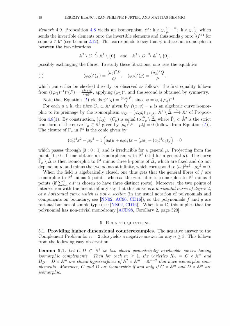
38 JÉRÉMY BLANC, JEAN-PHILIPPE FURTER, AND MATTIAS HEMMIG
Remark 4.9. Proposition 4.8 yields an isomorphism ψ∗ : k[x, y, 1g]'−→ k[x, y, 1
f] which
sends the invertible elements onto the invertible elements and thus sends g onto λf±1 forsome λ ∈ k∗ (see Lemma 2.12). This corresponds to say that ψ induces an isomorphismbetween the two fibrations
A2 \ C f→ A1 \ {0} and A2 \D g→ A1 \ {0},
possibly exchanging the fibres. To study these fibrations, one uses the equalities
(I) (ϕQ)∗(f) =(a0)2P
Q, (ϕP )∗(g) =
(a3)2Q
P,
which can either be checked directly, or observed as follows: the first equality followsfrom ((ϕQ)−1)∗(P ) = yf(x,y)
(a0)2, applying (ϕQ)∗, and the second is obtained by symmetry.
Note that Equation (I) yields ψ∗(g) = (a0a3)2
f, since ψ = ϕP (ϕQ)−1.
For each µ ∈ k, the fibre Cµ ⊂ A2 given by f(x, y) = µ is an algebraic curve isomor-phic to its preimage by the isomorphism ψQ = (ϕQη)|A2\∆ : A2 \ ∆
'−→ A2 of Proposi-tion 4.8(1). By construction, (ψQ)−1(Cµ) is equal to Γµ \ ∆, where Γµ ⊂ A2 is the stricttransform of the curve Γµ ⊂ A2 given by (a0)2P − µQ = 0 (follows from Equation (I)).The closure of Γµ in P2 is the conic given by
(a0)2x2 − µy2 − z(a0(µ+ a0a2)x− (µa1 + (a0)2a3)y
)= 0
which passes through [0 : 0 : 1] and is irreducible for a general µ. Projecting from thepoint [0 : 0 : 1] one obtains an isomorphism with P1 (still for a general µ). The curveΓµ \ ∆ is then isomorphic to P1 minus three k-points of ∆, which are fixed and do notdepend on µ, and minus the two points at infinity, which correspond to (a0)2x2−µy2 = 0.
When the field is algebraically closed, one thus gets that the general fibres of f areisomorphic to P1 minus 5 points, whereas the zero fibre is isomorphic to P1 minus 4points (if
∑3i=0 ait
i is chosen to have three distinct roots). Moreover, the two points ofintersection with the line at infinity say that this curve is a horizontal curve of degree 2,or a horizontal curve which is not a section (in the usual notation of polynomials andcomponents on boundary, see [NN02, AC96, CD16]), so the polynomials f and g arerational but not of simple type (see [NN02, CD16]). When k = C, this implies that thepolynomial has non-trivial monodromy [ACD98, Corollary 2, page 320].
5. Related questions
5.1. Providing higher dimensional counterexamples. The negative answer to theComplement Problem for n = 2 also yields a negative answer for any n ≥ 3. This followsfrom the following easy observation:
Lemma 5.1. Let C,D ⊂ A2 be two closed geometrically irreducible curves havingisomorphic complements. Then for each m ≥ 1, the varieties HC = C × Am andHD = D × Am are closed hypersurfaces of A2 × Am = Am+2 that have isomorphic com-plements. Moreover, C and D are isomorphic if and only if C × Am and D × Am areisomorphic.

EXCEPTIONAL ISOMORPHISMS BETWEEN COMPLEMENTS OF AFFINE PLANE CURVES 39
Proof. Denoting by f, g ∈ k[x, y] the geometrically irreducible polynomials that definethe curves C,D, the varieties HC , HD ⊂ A2 × Am = Am+2 are given by the samepolynomials and are thus again closed geometrically irreducible hypersurfaces. Theisomorphism A2\C '−→ A2\D extends then naturally to an isomorphism Am+2\HC
'−→Am+2 \HD.
If C and D are isomorphic, then HC and HD are isomorphic. The converse also holds,and is proven in [AHE72, Corollary (3.4)]. �
Corollary 5.2. For each ground field k and each integer n ≥ 3, there exist two geomet-rically irreducible smooth closed hypersurfaces E,F ⊂ An which are not isomorphic butwhose complements An \ E and An \ F are isomorphic. Furthermore, the hypersurfacescan be given by polynomials f, g ∈ k[x1, x2] ⊂ k[x1, . . . , xn] of degree 7 if the field admitsmore than 2 elements and of degree 13 if the field has 2 elements. The hypersurfacesE,F are isomorphic to C×An−2 and D×An−2 for some smooth closed curves C,D ⊂ A2
of the same degree.
Proof. It suffices to choose for f, g the equations of the curves C,D ⊂ A2 given byTheorem 3. The result then follows from Lemma 5.1. �
5.2. The holomorphic case.
Lemma 5.3. For each d + 1 distinct points a1, . . . , ad, ad+1 ∈ C, with d ≥ 3, thereexist two closed algebraic curves C,D ⊂ C2 of degree d2 − d+ 1 such that C and D arealgebraically isomorphic to C\{a1, . . . , ad−1, ad} and C\{a1, . . . , ad−1, ad+1} respectively,and such that C2 \ C and C2 \D are algebraically isomorphic.
In particular, choosing the points general enough, the curves C and D are not biholo-morphic, but their complements are biholomorphic.
Proof. The existence of C,D directly follows from Proposition 4.2. It remains to observethat C and D are not biholomorphic if the points are general enough. If f : C → Dis a biholomorphism, then f extends to a holomorphic map CP1 → CP1, as it cannothave essential singularities. The same holds for f−1, so f is just an element of PGL2(C),hence an algebraic automorphism of the projective complex line. Removing at least 4points of CP1 (this is the case since d ≥ 3) and moving one of them gives then infinitelymany curves up to biholomorphism. �
Corollary 5.4. For each n ≥ 2, there are algebraic hypersurfaces E,F ⊂ Cn which arecomplex manifolds, not biholomorphic but having biholomorphic complements.
Proof. It suffices to take polynomials f, g ∈ C[x1, x2] provided by Lemma 5.3, whose zerosets are smooth algebraic curves C,D ⊂ C2 not biholomorphic but having holomorphiccomplements. We then use the same polynomials to define E,F ⊂ Cn, which aresmooth complex manifolds that have biholomorphic complements and are biholomorphicto C×Cn−2 andD×Cn−2 respectively. It remains to observe that C×Cn−2 andD×Cn−2
are not biholomorphic. Denote by pC : C × Cn−2 → C and pD : D × Cn−2 → D theprojections on the first factor. If ψ : Cn−2 × C → Cn−2 ×D is a biholomorphism, thenpD ◦ψ : Cn−2×C → D induces, for each c ∈ C, a holomorphic map Cn−2 → D which hasto be constant by Picard’s theorem (since it avoids at least two values of C). Therefore,the map pD ◦ψ factors through a holomorphic map χ : C → D: we have pD ◦ϕ = χ◦pC .

40 JÉRÉMY BLANC, JEAN-PHILIPPE FURTER, AND MATTIAS HEMMIG
We get analogously a holomorphic map θ : D → C, which is by construction the inverseof χ, so C and D are biholomorphic, a contradiction. �
Appendix: The case of P2
In this appendix, we describe some results on the question of complements of curvesin P2 explained in the introduction. These are not directly related to the rest of the textand only serve as comparison with the affine case.
We recall the following simple argument, known to specialists, for lack of reference:
Proposition A.1. Let C,D ⊂ P2 be two geometrically irreducible closed curves suchthat P2\C and P2\D are isomorphic. If C and D are not equivalent, up to automorphismof P2, then C and D are singular rational curves.
Proof. Denote by ϕ : P2 99K P2 a birational map which restricts to an isomorphismP2 \ C '−→ P2 \ D. If ϕ is an automorphism of P2, then C and D are equivalent.Otherwise, the same argument as in Lemma 2.7 shows that both C and D are rational(this also follows from [Bla09, Lemma 2.2]). If C and D are singular, we are finished,so we can assume that one of them is smooth, and then has degree 1 or 2. The Picardgroup of P2 \ C being Z/ deg(C)Z, one finds that C and D have the same degree. Thisimplies that C and D are equivalent under automorphisms of P2. The case of lines isobvious. For conics, it is enough to check that a rational conic over any field is necessarilyequivalent to the conic of equation xy+z2 = 0. Actually, one may always assume that therational conic contains the point [1 : 0 : 0], since it contains a rational point. One mayfurthermore assume that the tangent at this point has equation y = 0. This means thatthe equation of the conic is of the form xy+u(y, z), where u is a homogenous polynomialof degree 2. Using a change of variables of the form (x, y, z) 7→ (x+ ay+ bz, y, z), wherea, b ∈ k, one may assume that the equation is of the form xy + cz2 = 0, where c ∈ k∗.Then, using the change of variables (x, y, z) 7→ (cx, y, z), one finally gets, as announced,the equation xy + z2 = 0. �
In order to get families of (singular) curves of P2 having the same complement, weexplicit here the construction of Paolo Costa [Cos12]. We obtain thus unicuspidal curvesof P2 which have isomorphic complements but which are non-equivalent under the actionof Aut(P2). We provide equations and give the details of the proof for self-containedness,and also because the results below are not explicitly stated in [Cos12].
Lemma A.2. Let k be a field. Let d ≥ 1 be an integer and P ∈ k[x, y] be a homoge-nous polynomial of degree d which is not a multiple of y. We define the homogeneouspolynomial fP ∈ k[x, y, z] of degree 4d+ 1 by the following formula, where w := xz− y2:
fP = zw2d + 2ywdP (x2, w) + xP 2(x2, w).
Denote by CP ,L,Q ⊂ P2 the curves of equations fP = 0, resp. z = 0, resp. w = 0, andby VP , VL, VQ ⊂ A3 their corresponding cones (given by the same equations). Then:(1) The polynomial fP is geometrically irreducible (i.e. irreducible in k[x, y, z]).(2) The rational map ψP : A3 99K A3 sending (x, y, z) to(
x, y + xP(x2w−1, 1
), z + 2yP
(x2w−1, 1
)+ xP 2
(x2w−1, 1
) )

EXCEPTIONAL ISOMORPHISMS BETWEEN COMPLEMENTS OF AFFINE PLANE CURVES 41
is a birational map of A3 that restricts to isomorphisms
A3 \ VQ'−→ A3 \ VQ, VP \ VQ
'−→ VL \ VQ and A3 \ (VQ ∪ VP )'−→ A3 \ (VQ ∪ VL).
Since ψP is homogeneous, the same formula induces a birational map of P2 thatrestricts to isomorphisms
P2 \ Q '−→ P2 \ Q, CP \ Q'−→ L \ Q and P2 \ (Q∪ CP )
'−→ P2 \ (Q∪ L).
Since [0 : 0 : 1] is the unique point of intersection between CP and Q, this proves inparticular that this point is the unique singular point of CP .
(3) Let λ be a nonzero element of k. Then, the rational map
ϕλ : (x, y, z) 7→(x+ (λ− 1)wz−1, y, z
)= (λx− (λ− 1)y2z−1, y, z)
is a birational map of A3 that restricts to automorphisms of A3 \ VL, VQ \ VL andA3 \ (VL ∪ VQ). The same formula yields then automorphisms of P2 \ L, Q \ L andP2 \ (L ∪Q).
(4) Set P (x, y) = P (λx, y) and κ = (ψP )−1ϕλψP . Then, the rational map κ restricts toan isomorphism A3 \ VP
'−→ A3 \ VP . In particular, κ also induces an isomorphismP2 \ CP
'−→ P2 \ CP .(5) For each homogeneous polynomial P ∈ k[x, y] of degree d which is not divisible by y,
the curves CP and CP are equivalent up to automorphisms of P2, if and only if thereexist some constants ρ ∈ k∗, µ ∈ k such that
P (x, y) = ρP (ρ2x, y) + µyd.
Proof. (1)-(2): As each rational map A3 99K A3, the rational map ψP yields a morphismof k-algebras (ψP )∗ : k[x, y, z]→ k(x, y, z). This sends x, y, z onto x, y+xP (x2w−1, 1), z+2yP (x2w−1, 1)+xP 2(x2w−1, 1). One also observes that (ψP )∗ fixes x and w. This impliesthat (ψP )∗ extends to an endomorphism of k[x, y, z, w−1], which is moreover an auto-morphism since (ψP )∗ ◦ (ψ−P )∗ = id. Extending to the quotient field k(x, y, z), one getsan automorphism of k(x, y, z), that we again denote by (ψP )∗, so ψP is a birational mapof A3 and induces moreover an isomorphism of A3 \ VQ, because (ψP )∗(k[x, y, z, w−1]) =k[x, y, z, w−1]. One then observes that (ψP )∗(z) = fPw
−2d where fP and w = xz−y2 arecoprime since fP (1, 0, 0) = P 2(1, 0) 6= 0. Let us also observe that VP ∩ VQ = {(x, y, z) ∈A3 | x = y = 0} and that VL ∩ VQ = {(x, y, z) ∈ A3 | y = z = 0}. Hence ψP restrictsto an isomorphism of surfaces VP \ VQ
'−→ VL \ VQ. This implies that VP and CP arerational, and that fP is geometrically irreducible, proving (1). This also implies that ψPrestricts to an isomorphism A3 \ (VQ ∪ VP )
'−→ A3 \ (VQ ∪ VL). As ψP is homogeneous,one gets the analogous results by replacing A3, VP , VL, VQ by P2, CP , L, Q respectively.
(3): One checks that ϕλ ◦ ϕλ−1 = id, so ϕλ is a birational map of A3, which restrictsto an automorphism of A3 \ VL, since the denominators only involve z. Moreover,(ϕλ)
∗(w) = λw (where (ϕλ)∗ is the automorphism of k(x, y, z) corresponding to ϕλ),
so the surface VQ \ VL is preserved, hence ϕλ restricts to automorphisms of A3 \ VL,VQ \ VL and A3 \ (VL ∪ VQ). Since ϕλ is homogeneous, the same formula yields thenautomorphisms of P2 \ L, Q \ L and P2 \ (L ∪Q).
(4): By (2)-(3), the transformation κ = (ψP )−1ϕλψP restricts to an isomorphismA3 \ (VQ ∪ VP )
'−→ A3 \ (VQ ∪ VP ). Let us prove that with the special choice of P that

42 JÉRÉMY BLANC, JEAN-PHILIPPE FURTER, AND MATTIAS HEMMIG
we have made, then κ restricts to an isomorphism A3 \ VP'−→ A3 \ VP . For this, we
prove that the restriction of κ yields the identity automorphism on VQ \VP = VQ \VP =VQ \ {(x, y, z) ∈ A3 | x = y = 0}. We compute
ϕλψP (x, y, z) =(x+ (λ− 1)w2d+1f−1
P , y + xP (x2, w)w−d, fPw−2d)
which satisfies (ϕλψP )∗(w) = (ϕλ)∗(w) = λw. To simplify the notation, we write δ =
(λ− 1)w2d+1f−1P and get that κ(x, y, z) = (ψP )−1ϕλψP (x, y, z) is equal to(x+ δ, y + xP (x2, w)w−d − (x+ δ)P
(λ−1(x+ δ)2w−1, 1
), z + ζ
)for some ζ ∈ k(x, y, z). Since P (x, y) = P (λx, y), the second component is
κ∗(y) = y +xP (x2, w)− P ((x+ δ)2, w)(x+ δ)
wd.
As wd+1 divides the numerator of δ, one can write κ∗(y) as y + w(fP )−nR, for someR ∈ k[x, y, z] and n ≥ 0. Similarly, κ∗(x) = x + wf−1
P S, where S ∈ k[x, y, z]. Sinceκ∗(w) = λw, we get
λw = (x+ wf−1P S)(z + ζ)− (y + wf−nP R)2
which shows that ζ(x+wf−1P S) = wf−mP T for some T ∈ k[x, y, z], m ≥ 0, hence one can
write κ∗(z) = z + ζ = z +wf−mP T for some T ∈ k[x, y, z] and m ≥ 0. This shows that κis well defined on VQ \ VP = VQ \ VP = VQ \ {(x, y, z) ∈ A3 | x = y = 0} and restricts tothe identity on this surface.
Since κ is homogeneous, the isomorphism A3 \VP'−→ A3 \VP also induces an isomor-
phism P2 \ CP'−→ P2 \ CP , which fixes pointwise the curve Q \ CP = Q \ CP .
(5): Suppose first that P (x, y) = ρP (ρ2x, y) + µyd for some ρ ∈ k∗, µ ∈ k. Define thetransformation α ∈ GL3(k) by
α(x, y, z) = (x, ρy − µx, ρ2z − 2ρµy + µ2x)
and the birational transformation s ∈ Bir(A3) by s = ψPα(ψP )−1. Let us note thats∗ = (ψ∗P )−1α∗ψ∗
P. One checks that α∗(w) = ρ2w, from which we get s∗(w) = ρ2w. The
equality
α∗(ψ∗P
(y)) = α∗(y + xP (x2w−1, 1)) = ρy − µx+ xP (ρ−2x2w−1, 1)= ρy + ρxP (x2w−1, 1) = ρψ∗P (y)
gives us s∗(y) = ρy. The relation z = x−1(w − y2) joined to the equality s∗(x) = x nowproves us that s∗(z) = ρ2z. But we have (ψP )∗(z) = fPw
−2d and (ψP )∗(z) = fPw−2d, so
that we get α∗(fPw−2d) = ρ2fPw
−2d. In turn, this latter equality yields us
α∗(fP ) = ρ4d+2fP .
This shows that α induces an automorphism of P2 sending CP onto CP .Conversely, suppose that there exists τ ∈ Aut(P2) sending CP onto CP .We begin by proving that τ preserves the conicQ. Since CP \Q ' CP \Q ' L\Q ' A1,
the irreducible conic Q ⊂ P2 intersects CP (respectively CP ) in exactly one k-point, theunique singular point [0 : 0 : 1] of CP (resp. CP ). The irreducible conic τ(Q) intersectsthus also CP into one k-point, namely [0 : 0 : 1]. Let us observe that this implies thatτ(Q) = Q. One first notices that CP \ {[0 : 0 : 1]} ' A1, so there is one k-point at

EXCEPTIONAL ISOMORPHISMS BETWEEN COMPLEMENTS OF AFFINE PLANE CURVES 43
each step of the resolution of CP . We can then write q1 = [0 : 0 : 1] and define asequence of points (qi)i≥1 such that qi is the point infinitely near qi−1 belonging to thestrict transform of CP , for each i ≥ 2. Denote by r the biggest integer such that qrbelongs to the strict transform of Q and by r′ the biggest integer such that qr′ belongsto the strict transform of τ(Q). Bézout Theorem yields (since Q and τ(Q) are smooth)
r∑i=1
mqi(CP ) = deg(Q) deg(CP ) = deg(τ(Q)) deg(CP ) =r′∑i=1
mqi(CP ),
which yields r = r′. On the blow-up X → P2 of q1, . . . , qr, the strict transform ofthe curve CP is then disjoint from those of Q and τ(Q), which are linearly equivalent.Assume by contradiction that we have τ(Q) 6= Q. Then, we claim that the stricttransform of any irreducible conic Q′ in the pencil generated by Q and τ(Q) is alsodisjoint from the strict transform of CP . Indeed, we first note that CP and Q′ have nocommon irreducible component since CP is an irreducible curve whose degree satisfies
degCP ≥ 5 > 2 = degQ′.
Finally, since the (infinitely near) points q1, . . . , qr belong to both Q′ and CP and sincewe have the equality
∑ri=1mqi(CP ) = deg(Q′) deg(CP ), the curves Q′ and CP do not
have any other common (infinitely near) point.Choose now a general point q of P2 which belong to CP \ {q1} ' A1 and choose the
conic Q′ in the pencil generated by Q and τ(Q) which passes through q. Then, the stricttransforms of Q′ and CP intersect in X (at the point q). This contradiction shows thatQ is preserved by τ .
Since τ ∈ Aut(P2) = PGL3(k) fixes the point [0 : 0 : 1] (which is the unique singularpoint of both CP and CP ) and preserves the line x = 0 (which is the tangent line ofboth CP and CP at the point [0 : 0 : 1]), it admits a (unique) lift α ∈ GL3(k) which istriangular and which satisfies α∗(x) = x. This means that α is of the form:
α : (x, y, z) 7→ (x, ρy − µx, γz + δy + εx),
for some constants ρ, µ, γ, δ, ε ∈ k (satisfying ργ 6= 0). Since α∗(w) is proportional to w,we get γ = ρ2, δ = −2ρµ and ε = µ2, i.e. α is of the form
α : (x, y, z) 7→ (x, ρy − µx, ρ2z − 2ρµy + µ2x).
Set s := ψPα(ψP )−1 ∈ Bir(A3). Since α∗(w) = ρ2w, we also get s∗(w) = ρ2w. Since(ψP )∗(z) = fPw
−2d, (ψP )∗(z) = fPw−2d and since α∗(fP ) and fP are proportional, the
fractions s∗(z) and z are also proportional. Therefore, there exists a nonzero constantξ ∈ k such that
(J) s∗(x) = x, s∗(w) = ρ2w, s∗(z) = ξz.
Moreover, s induces a birational map s of P2 which is an automorphism of P2 \Q, because the same holds for α, ψP and ψP . Let us observe that s is in fact anautomorphism of P2. Indeed, otherwise s would contract Q to one point. This isimpossible: Since s preserves the two pencils of conics given by [x : y : z] 7→ [w : x2]and [x : y : z] 7→ [w : z2], which have distinct base-points [0 : 0 : 1] and [1 : 0 : 0],these base-points are fixed by s. Hence, there exist some constants ζ, η, θ ∈ k such that

44 JÉRÉMY BLANC, JEAN-PHILIPPE FURTER, AND MATTIAS HEMMIG
s∗(y) = ζx + ηy + θz. Hence (J) gives us ζ = θ = 0, i.e. s∗(y) = ηy. But the equalitys = ψPα(ψP )−1 yields us ψPα = sψP and by taking the second coordinate we get
(ρy − µx) + xP(ρ−2x2w−1, 1
)= (ψPα)∗(y) = (sψP )∗(y) = η
(y + xP
(x2w−1, 1
))which yields ρ = η and P (ρ−2x2w−1, 1) = ρP (x2w−1, 1) + µ. By substituting ρ−2y +x−1y2 for z and by noting that w(x, y, ρ−2y + x−1y2) = ρ−2xy, we obtain P (xy−1, 1) =ρP (ρ2xy−1, 1) +µ, which is equivalent to P (x, y) = ρP (ρ2x, y) +µyd, as we wanted. �
The construction of Lemma A.2 yields, for each d ≥ 1, families of curves of degree4d+ 1 having isomorphic complements. These are equivalent for d = 1, at least when kis algebraically closed (Lemma A.2(5)), but not for d ≥ 2. One can now easily provideexplicit examples:
Corollary A.3. Let d ≥ 2 be an integer. Set P = xd +xd−1y and w = xz− y2 ∈ k[x, y].All curves of P2 given by
zw2d + 2ywdP (λx2, w) + xP 2(λx2, w) = 0
for λ ∈ k∗, have isomorphic complements and are pairwise not equivalent up to auto-morphisms of P2.
Proof. The curves correspond to the curves CP (λx,y) of Lemma A.2 and have thus iso-morphic complements by Lemma A.2(4). It remains to show that if CP (λx,y) is equivalentto CP (λx,y), then λ = λ. Lemma A.2(4) yields the existence of ρ ∈ k∗, µ ∈ k such thatP (λx, y) = ρP (ρ2λx, y) + µyd. Since d ≥ 2, both P (λx, y) and ρP (ρ2λx, y) do not havecomponent with yd, so µ = 0. We then compare the coefficients of xd and xd−1y and get
λd = ρ(ρ2λ)d, λd−1 = ρ(ρ2λ)d−1,
which yields λ = ρ2λ, whence ρ = 1 and λ = λ as desired. �
References
[AHE72] Abhyankar Shreeram Shankar, Heinzer William, Eakin Paul, On the uniqueness of thecoefficient ring in a polynomial ring, J. Algebra 23 (1972), 310–342. 5.1
[AC96] Artal-Bartolo Enrique, Cassou-Nogués Pierrette, One remark on polynomials in two vari-ables, Pacific J. Math. 176 (1996), no. 2, 297–309. 4.9
[ACD98] Artal-Bartolo Enrique, Cassou-Nogués Pierrette and Dimca Alexandru, Sur la topologiedes polynômes complexes, Progress in Mathematics, 162 (1998), 317–343. 4.9
[Bla09] Blanc Jérémy, The correspondence between a plane curve and its complement, J. ReineAngew. Math. 633 (2009), 1–10. 1, 5.2
[BS15] Blanc Jérémy, Stampfli Immanuel, Automorphisms of the plane preserving a curve, Al-gebr. Geom. 2 (2015), no. 2, 193–213. 2.9, 2.3
[CD16] Cassou-Noguès Pierrette, Daigle Daniel, Rational polynomials of simple type: a combi-natorial proof, to appear in Proceedings of Kyoto Workshop 2014, Advanced Studies inPure Mathematics (ASPM). 4.9
[Cos12] Costa Paolo, New distinct curves having the same complement in the projective plane,Math. Z. 271 (2012), no. 3-4, 1185–1191. 1, 5.2
[Dai91] Daigle Daniel, Birational endomorphisms of the affine plane, J. Math. Kyoto Univ. 31(1991), no. 2, 329–358. 2.4
[Gan85] Ganong Richard, Kodaira dimension of embeddings of the line in the plane, J. Math.Kyoto Univ. 25 (1985), no. 4, 649–657. 2.30

EXCEPTIONAL ISOMORPHISMS BETWEEN COMPLEMENTS OF AFFINE PLANE CURVES 45
[Kam79] Kambayashi Tatsuji, Automorphism group of a polynomial ring and algebraic group actionon an affine space, J. Algebra 60 (1979), no. 2, 439–451. 2.9
[KM83] Kumar Mohan, Murthy Pavaman, Curves with negative self intersection on rational sur-faces, J. Math. Kyoto Univ. 22 (1983), no. 4, 767–777. 2.30
[Kra96] Kraft Hanspeter, Challenging problems on affine n-space, Séminaire Bourbaki, Vol.1994/95. Astérisque No. 237 (1996), Exp. No. 802, 5, 29–317. (document), 1, 3.6
[NN02] Neumann Walter D., Norbury Paul, Rational polynomials of simple type, Pacific J. Math.204 (2002), no. 1, 177–207. 4.9
[Pol16] Poloni Pierre-Marie, Counterexamples to the Complement Problem,https://arxiv.org/abs/1605.05169 1, 1, 1
[Rus70] Russell Peter, Forms of the affine line and its additive group, Pacific J. Math. 32 1970527–539. 2.31
Jérémy Blanc, Universität Basel, Departement Mathematik und Informatik, Spiegel-gasse 1, CH-4051 Basel, Switzerland
E-mail address: [email protected]
Jean-Philippe Furter, Dpt. of Math., Univ. of La Rochelle, av. Crépeau, 17000 LaRochelle, France
E-mail address: [email protected]
Mattias Hemmig, Universität Basel, Departement Mathematik und Informatik, Spiegel-gasse 1, CH-4051 Basel, Switzerland
E-mail address: [email protected]