Excel 97 Basic - clearcutcomputing.com Basic.pdf · Microsoft Excel – Basic Skills Paul J. Montenero Page – 3 Adjusting column sizes (and row sizes too) There are two ways to

Microsoft Excel – Basic Skills

Paul J. Montenero Page – 1

The "Anatomy" of the EXCEL window The typical EXCEL window will look similar to that shown below. It is possible to customize your own display, but that is a topic for discussion later on.

Title Bar – Displays the name of the program (Microsoft Excel), and usually, the name of the Workbook that you are currently working on. The default workbook at startup is named "Book1." Main Menu – Contains every option available in EXCEL. Tool Bar(s) — Populated with buttons; which are shortcuts to some of the menu choices. Formula Bar — Is where you enter the "contents" of each "cell." Cells can contain numbers, text or mathematical formulas. Worksheets — Are separate sets of cells (more on this a bit later). A "Worksheet" is also referred to as a "Spreadsheet." Status Bar — Shows helpful messages while you use various features of Excel An Excel Spreadsheet is made up of Rows and Columns. Rows are represented by Numbers and Columns are represented by Letters. An intersection of a ROW and a COLUMN is known as a CELL. Each cell has a unique address. In the graphic above, the current cell, the cell that is highlighted is referred as A1.

TITLE BAR

MENU BAR

TOOL BAR(S)

FORMULA BAR

STATUS BAR

WORKSHEETS



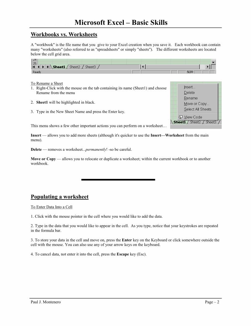
Workbooks vs. Worksheets A "workbook" is the file name that you give to your Excel creation when you save it. Each workbook can contain many "worksheets" (also referred to as "spreadsheets" or simply "sheets"). The different worksheets are located below the cell grid area.

To Rename a Sheet 1. Right-Click with the mouse on the tab containing its name (Sheet1) and choose

Rename from the menu 2. Sheet1 will be highlighted in black. 3. Type in the New Sheet Name and press the Enter key. This menu shows a few other important actions you can perform on a worksheet… Insert — allows you to add more sheets (although it's quicker to use the Insert—Worksheet from the main menu). Delete — removes a worksheet...permanently! -so be careful. Move or Copy — allows you to relocate or duplicate a worksheet; within the current workbook or to another workbook. Populating a worksheet To Enter Data Into a Cell 1. Click with the mouse pointer in the cell where you would like to add the data. 2. Type in the data that you would like to appear in the cell. As you type, notice that your keystrokes are repeated in the formula bar. 3. To store your data in the cell and move on, press the Enter key on the Keyboard or click somewhere outside the cell with the mouse. You can also use any of your arrow keys on the keyboard. 4. To cancel data, not enter it into the cell, press the Escape key (Esc).



Adjusting column sizes (and row sizes too) There are two ways to adjust the widths of a column: Precise — use the menu Format—Column—Width By hand —РMove the mouse pointer between two column labels until the mouse pointer changes to a At this point, click-and-hold the mouse button and move the mouse left or right to increase or decrease the width of the column. You'll note that this adjusts the width of the column to the left of the pointer. This process is similar to adjusting row heights...try it! Editing cells To Cut, Copy or Paste an entire cell (or rang of cells), select the cell and use the Edit menu. Notice that on the Edit menu, what's to the left and right of the menu choice. On the left is the Tool Bar button that would execute the same function as that menu choice. On the right is the keyboard shortcut to do the same function. For example, to copy the selected cell, you could also click the "two papers" icon on the Tool bar or you could have held down the control key (Ctrl) and pressed the "C" key on the keyboard. Note that not all of the menu choices have alternatives. You can also move a cell with the mouse. The selected cell will have a thick box around it. If you carefully move the mouse over the border of this box, the pointer will change to an arrow. While the arrow is visible, click-and-hold the left mouse button and move the mouse to drag the cell to a new location. When you let go of the button, the cell contents will be relocated. To replace the contents of a cell, select it and type the new data. When you press the Enter key, the old contents will be replaced with the new. To edit the contents of a cell, select it and click in the formula box. You should notice that when you move the pointer over the formula box, it changes to an "I-beam" -similar to that used in word processors. Edit the data and press the Enter key, the old contents will be revised. Selecting multiple cells — for many functions (such as cut, copy, paste and move), you can select a "range" of cells.

Contiguous selection Scattered selection 1. Point to a cell 1. Click on a cell 2. Click and hold the mouse button 2. Hold down the Ctrl ѫey 3. Move the mouse to another cell 3. Click on one or more additional cells

You may also select an entire row or column simply by clicking on the header of the row or column. Inserting & Deleting Rows and Columns You can add or remove rows and columns as needed. The easiest way to do so is to right-click on the row or column header and from the menu, choose Insert or Delete. When add a row, all existing rows below it are shifted downward. When adding a column, all existing columns shift to the right of it.



AutoFill to Fill Cells When there is a consecutive series of Labels or numbers to be entered — such as Quarters, Years or Days — Excel has a Feature that allows us to enter only the first value and then fill the rest of the values in by dragging with the left mouse button. In the Example Below, Excel will fill in QTR 2, QTR 3 and QTR 4. 1. Type in the first label for the series I.E. QTR 1 2. Place your mouse pointer in the lower right hand side of the cell, until it takes the shape of a +. 3. Hold the left mouse button down and drag the pointer until all cells are filled. As you drag the pointer a gray border will appear along the cells. Seen below. 4. Once all the cells are selected, release the mouse. Creating Custom AutoFill Lists 1. Click on Tools from the Main Menu. 2. Move down the menu with the mouse and click on Options, the following window will appear, make sure the custom lists tab is selected. If the Custom Lists tab is not selected, click on it with the mouse. 3. To create a New List, click on New List and click on ADD. 4. Type in the items of your list all separated with a comma. When you are done typing your items click on OK. 5. Test the List that you created by Typing in the first value of the list and dragging the mouse pointer across the columns to complete the list. Undo — the "forgiving" command You shouldn't become too concerned about making errors and executing functions you did not intend — because you always have the "undo" function at you disposal. It's found on the edit menu, and you can run it repeatedly to work backwards over several tasks that you may have done. And if you undo something you wanted to keep, you can always use its cousin, the "redo" function!



Navigating Excel Usually, you will be entering large amounts of data into the many cells of an Excel worksheet. If you had to click on each cell before you entered the data you would be at it a longer time than necessary. Take advantage of the following keyboard navigation tools while you type: Enter key unless you changed the program's options, pressing the Enter key should move you one cell

downward. Shift—Enter moves one cell upward Tab key moves one cell to the right Shift—Tab moves one cell to the left Arrow keys moves one cell in the direction of the arrow Page Down moves one screen downward Page Up moves a full screen upward Home key moves to the first column in the current row Ctrl—Home moves to cell A1 —or— to the upper left cell in a range Ctrl—End moves to the lower right of a range Ctrl—Arrow moves to the end of string of blank or filled cells Adjusting Your View

If you have multiple workbooks open at the same time, you can use the Window menu to ar-range them neatly...

...or you can switch amongst the open workbooks by selecting the one you want from the bottom of the Window menu.

If your worksheet is larger than the viewing window (a common prob-lem to 12-month financial tables), use the zoom box on the Standard Tool bar.



For the bulk of this course, we'll produce a spreadsheet to report the sales of three stores for a Long Island company. You can see the finished chart later on in this booklet. Let's start by typing in the numbers in the figure below.

Creating Formulas Based on the example above, we want to create a formula that will add the store totals for Monday and place in the answer in Cell B8. In a formula you must reference the cells that you want to perform the formula on by its cell address. For Example: 1. First we need to click in cell B8. 2. Every formula must start with an equal sign (=) so we must type that in, then we must type the cell address in

for each cell that we would like to add together. 3. The formula should look like this =B5+B6+B7 4. Press the Enter key and your result of 1935.71 should be shown in cell B8. If you select cell B8, yoѵ'll see the

formula you typed in the Formula box. "Point & Shoot" method You need not type in the entire formula on the keyboard. Alternatively, you can use your mouse to click on the cells used in your formula. Let's do Tuesday's total using this method: 1. Click on cell C8 and press the = key on the keyboard. 2. Now click on cell C5. Note how that cell reference is inserted into your formula. 3. Press the + key on the keyboard and then click on cell C6. 4. Repeat step 3 for cell C7. 5. Finish your formula by pressing the Enter key.



With either method, this formula could become quite cumbersome if we had a column of, say, 20 numbers or more! For adding columns of numbers, we could use the SUM function in EXCEL. A function is a short cut that we can use to accomplish the same thing as a formula with less typing involved. The syntax for using the SUM function is as follows: =SUM(first cell of range : last cell of range) For example Instead of using the Formula =B5+B6+B7 To get the total sales for Monday, we could type in =SUM(B5:B7) Where B5 is the first cell that we want to add and B7 is the last cell that we want to add. Point & Shoot Method Most people would have used the Point & Shoot method along with the Tool bar. Delete the formula you just typed and let's start over: 1. Click on cell B8 2. Press the Σ button on the Tool bar — this is the SUM function button 3. EXCEL functions are intelligent enough in that they "guess" at what you want to do. Here, you'll notice that a

box of "marching ants" surrounds the range of cells EXCEL thinks you want to add. Just press the Enter key and you're done!

EXCEL has many functions like the SUM function available for your use. We'll explore a few later on in the course. The SUM function, however, is the only one with its own button on the Tool bar. Totals for the rest of the columns For the final step of this example, we will copy this formula to the rest of the day totals. To Copy Formulas 1. Click in the cell where the original formula should be located. 2. Once the first formula is typed in and entered into the cell, click-and-hold on the box in the lower right hand

corner of the cell and drag the mouse pointer to the cells where you would like the formulas copied. 3. Let go of the mouse button, and notice that your formula has been intelligently pasted in each column. I used

the word "Intelligently," because if you examine the formula for Wednesday, for example, you'll see that the cell references changed from B5:B7 to D5:D7. Which is what it should be to correctly add the Wednesday numbers! We will discuss this topic further when we cover "Absolute Cell References" — that is holding the cell references steady during a copy process.

You can total the numbers across as well. The process is similar. Practice this by entering the total for each office and place them in the column to the right of Friday's numbers. You can call the heading of this column “Site Total.”



Absolute Cell References As you’ve seen, when Excel copies formulas, it uses relative cell addressing. This means that as we copy a formula, Excel automatically changes the column and row labels. In our example, we want to track the change in sales from day-to-day. In the row below the Daily Total, label the row “Increment” as shown in the figure below. Then in cell C9, type the following formula: =C8-B8 Now copy that formula to the right (using whatever method you’re comfortable with) and examine the formulas. You should see that cell D9=D8-C8; cell E9=E8-D8; etc. Notice that the row and column labels incremented.

But, you may have a need in your a spreadsheet where this is not desired. For example, perhaps you have a tax rate in one cell that needs to be used in a formula for each line item. In order to do this, we must make the cell reference absolute. Let’s return to our example. The entire chain of stores has a daily target of $2,500 to which they measure their success. In the upper left corner of the sheet, enter the label “Daily Average” and below it the value 2,500 (as shown above. Row 10 of the figure above is where will place the formula that measures the daily success. As shown, label the row “Actual vs. Target.” In cell B10, type the following formula: =B8-A2 Now try copying this formula to the right...examine the formulas in each cell to see why they failed in all but cell B10. The formulas would have worked if the reference to A2 had stayed constant. We can instruct Excel to hold this reference steady by prefixing the column and row labels with a $ as such: =B8-$A$2 Type this formula into cell B10 and copy it to the right. Now your results should be perfect...check the formulas to see for yourself. As a shortcut, we could have gone to the formula bar and clicked anywhere on the cell address we want to add the absolute reference tags to, and press the F4 key on the keyboard. The $ symbols will be added. If you press repeatedly, you’ll see different forms of this occur: F4 —> $F$4 —> F$4 —> $F4. The last two cases are for more advanced uses and won’t be covered here. I will say, that in a nutshell, the $ holds only the label to it’s immediate right steady during formula copying. You may want to experiment with this on your own and refer to the Excel manual or help files.



Let’s add in one more row of formulas before we format our spreadsheet. In row 11, we want to track the percent of that day’s total vs. the weekly total. In cell B11, the formula would simply be: =B8/G8. Your answer should be some enormous decimal fraction. We’ll format this soon. Copy the formula thorough cell F11. Now enter similar formulas in column H for the percentages of each store’s sales vs. the weekly total. One last topic before we format our work...mathematical operators. We have already used three of the four basic mathematical operators in our sheet: addition, subtraction and division. Below is the symbol to use for all four (including the one we left out: multiplication): + addition =B5+B6+B7 - subtraction =B5-B4 * multiplication =B4*B5 / division =B8/G8 Parenthesis can be used for more complicated formulas. For example, the percent of the Amityville site total vs. the grand total for the week (cell H5) could be written as: =(B5+C5+D5+E5+F5)/(B8+C8+D8+E8+F8), Spreadsheet Formatting – Method 1: Using the Tool Bar 1. Cell Alignment — buttons are provided on the Tool bar to center, left or right justify cell contents. In this

example, we want to center the days of the week. 2. Changing the Font — in Excel, we have almost as much control over the font as we have in a word

processing program such as Microsoft Word. We can format many cells at once. Select the fourth row in this example, and use the Tool bar buttons marked "B" and "U" to format the text as bold, underlined.

3. Column Width — By now, you should notice that the heading "Wednesday" is too wide for its cell. Rather

than changing the width of that column alone, we want a uniform appearance across several columns. First select the five columns containing the days of the week and use what you learned for adjusting a column width to optimize the width for Wednesday. You will notice that all columns selected are now the same width.

4. Number Formatting — Many quick formatting tasks can be accomplished through the Tool bar.

Currency — Formats numbers in the selected cells for decimal dollars $(1,234.56) Percent — Formats decimal numbers as percents: 0.12 ==> 12% Commas — Similar to the currency format button, but no dollar sign: (1,234.56) Increase/Decrease Decimal — Notice that in the previous buttons, the number of decimal places are pre-determined for you. You can show more or less decimal places of the selected cell(s) by clicking on these buttons.

5. Borders —The reader of this chart should be drawn to important results contained in this chart. Therefore, we

would want our Daily Total row to stand out. One of the things we will do is to place a border on the top and bottom of the cells. Select the seven cells from A8 through G8 and use the "borders "button on the Tool bar to select an appropriate set of borders.

6. Shading — The "Site Total" column is another important area we want our reader to focus on. Here, we'll use

a different attention-grabbing method. Select the five cells from G5 through G8 and use the "Fill Color" button to select a background color for the cells.

7. Font Coloring — Similar to the shading function just discussed, we can change the color of the font itself.

Select the Daily Average cells: A1 and A2. Use the Font Color button to change that color to red.



Your Spreadsheet should now look something like the figure above. Are you proud of your work? Good...now let’s clear all the formatting by selecting all the cells and choosing from the menu Edit—Clear—Formats. Try not to be too depressed, we’re going to use another method to format our spreadsheet. Spreadsheet Formatting – Method 2: Using the Format — Cells Menu An alternate, and more powerful way to format your work is through the Format Cells command. First, as usual, select the cell(s) you wish to format and choose form the menu: Format — Cells. The window below will appear. The different types of formatting available are divided into six tabs: Number, Alignment, Font, Border, Pattern and Protection. All but the Protection tab is explained below (the concept of protecting a cell or sheet is an advanced topic and is not covered here). Number — For each category on the left, various

formatting controls are presented on the right. Shown at the right is the Currency settings. It allows you to control how many decimal places to display, the type of currency symbol to use (if you are working in foreign currencies), and the display handling of negatives. As you can see, you can format the display to show negative numbers in red (bringing back to life, the phrase, “in the red”). Even though most printers, in use in an office environment today, only print in black, it is still valuable to use a setting for red negatives; it makes visual validation of your work, on screen, easier. The other categories we will cover in this course are Date (later on) and Percentage (and perhaps Special or Custom — briefly). Feel free to experiment with the others



Alignment — The Horizontal setting is just like the alignment buttons on the Tool bar. But, if you’ve changed the height of your rows, you can adjust the Vertical alignment of your cell contents. Additionally, you have several controls to handle long entries in cells — usually good for text: column headings and notes.

Font — Most of this is replicated on the Tool bar.

Additional controls include a variety of underlines, and other effects.

Borders — As opposed to the Tool bar button for setting borders, you have many more variations available to you from this screen, including colors and line styles.

Patterns — Change the cell background to another color;

even add a pattern to the background from the Patterns tab. On popular method of creating a striking effect on a spreadsheet is to create a title of text that is colored white and has a cell background of black or gray .



Printing Basics Print Preview After you’ve create your masterpiece, you’ll most likely want to print it. Before printing your work, it is a good idea to view it through Print Preview. You can access the Print Preview from the File menu or the corresponding Tool bar button. Page Setup Use the Page Setup to adjust the variables involved in printing. Here you can modify Margins, Orientation and add Headers and Footers. Different programs have different features on the their page setup screens. Some put these feature in different places on their Page Setup windows. For this conversation, we'll discuss only Margins and Orientation the two most common denominators usually found in all programs. Page Setup is usually found on the File menu. The screens below are from Microsoft Word.

Page Tab Orientation Orientation refers to the layout of the paper. Normally we write and print our work on an 8-1/2 x 11 inch piece of paper in Portrait orientation. But if we rotate the paper 90 degrees, we call it Landscape. Portrait

Landscape Scaling A feature not found in many programs is the scaling feature. This allows you shrink those wide spreadsheets (the 12-month variety) so they can fit on one piece of paper.

A

A

Margins Margins are shown in inches. The four most common margins are Top, Bottom, Left and Right. This sets the boundaries of the printing from the edges of the paper. NOTE: Before setting any margin to a very small

value (such as 0.25"), check your printer documentation. Many printers have a region where they can't print to.

Another good effect to employ is to Center the spreadsheet on the page.



Sheet Tab Print area You may have noticed that your print preview included some cells you didn’t want, or excluded others you did want. The way to control what gets printed is to specify the print area. In our sheet, we may want to exclude that Daily Average information. To do so, we need to specify the range of cells to print as: $A$4:$H$11 Print titles If your spreadsheet is longer or wider than one sheet of paper, You may want the row containing the column headings to print at the top of each page. In the Rows to repeat at the top box, enter: $5:$5 Repeat the process for any columns you want repeated in the Columns to repeat at left box. The absolute cell references are a good idea in case you insert any rows or columns later on...your print areas won’t shift. In lieu of typing, you could click-and-drag to select the ranges needed. Header/Footer Tab If you’re in a hurry, Excel offers a small assortment of headers and footers for you to choose from. Simply click on the drop-down arrows in each section and make your selection. Creating a Custom Header or Footer Alternatively, you can create your own customized Header and Footer. Click on Custom Footer or Custom Header. The following dialog box will appear. The Header/Footer section is divided into thirds. Based on where you want the components of your Header/Footer to appear, click with the mouse in one of the selections. There are several tools that we can use to create our Header/Footer. These tools are labeled in the figure to the right.

Font

Date

Time

File Name

Sheet Name

Page #

Tot Pgs



Saving your Workbook To save your workbook, choose File—Save from the menu or click the Save button on the Tool bar. If you are saving a new workbook for the first time — or you are saving a copy of the current workbook under another name — the Save As dialog window (shown at the right) will appear. The easy thing to do (and most necessary) is to simply give your workbook a name and type it into the File name box near the bottom of the window. But, you should take note where this file will be saved...look in the Save in box at the top of the window. In the example illustration above, the file is placed in an Excel folder that lives where? To find out where, click the pull-down arrow on the right of the box. The entire path, describing the location of the Excel folder, is shown in a tree format. As

indicated in the figure at the right. Click on a folder in the tree to move to that location. Then in the large box, you may see other folders to choose from. You can double-click one of those folders to open it.

You can also create a new sub-folder in the current folder by clicking the Create New Folder button at the top of this window. NOTE: Most computers, by default store the files created by the programs

installed on it in the My Documents folder. Lastly, you could change the format of the workbook you save so it can be read by other programs such as Lotus 1-2-3 or Quattro Pro. At the bottom of this window is a box labeled Save as type. Click the pull-down arrow to the right of this box to display a scrolling list of choices. Choose the desired format and then click the Save button. Note, however, that not all spreadsheet programs have the capabilities of Excel, so some of your formulas and formatting may be simplified in the other program. NOTE: The default format is the latest version of Excel, of course, so unless you are sharing this worksheet with a

non-Excel computer, you do not need to change this setting.



Charts & Graphs Excel offers a very quick way to create a chart — through the use of the Chart Wizard. To access it, choose Insert—Chart from the menu or click the Chart Wizard button on the Tool bar. The window that appears lets you select the Chart type in the left panel, and then specify the Chart sub-type (the exact format to be inserted in your worksheet) in the right panel. For this basic course, we’re going to cover only two of the Chart types: Column and Pie. The charting capabilities of Excel are extremely detailed and we could several classes just on this topic, as many of the chart elements are adjustable. But for this basic course, we want Excel to do most of the work for us. Hence, the best way to employ the Chart Wizard is to follow the general steps below:

1. Tell Excel what “data” we wish to create a chart from.

2. Start the Chart Wizard and select the chart style we want.

3. Click the Finish button. And PRESTO! Our chart appears in a box with control handles (those eight little squares on the perimeter of the box that we use to re-size it. We can move the chart anywhere we want on the sheet by using the “click-and-drag” technique.



Column Chart Following the steps on the previous page, first we need to tell Excel what data we want to chart. To do this we select a range of cells — be sure to include any column and row labels as they will be interpreted by the Chart Wizard. In the figure below, the correct range is shown. Note that I did not select the calculated totals. Now start the Chart Wizard, choose Column charts and select the first chart. Click the Finish button and you should see the chart as shown below. Move it to left to make room for the next chart we will add.



Pie Chart Unlike the Column chart in the previous example, where we could simultaneously display several “series” of data (multiple stores), a Pie chart is used to display the breakdown of only one series. So we can only select one store or row. But we still want our column headings (the days of the week) to be used in the chart. We can accomplish this by selecting the data row and the headings row together in a “staggered selection.”

1. First, lets select the range of cells defining the store’s data (from A6:F6).

2. Then hold the Ctrl key down on the keyboard and select the range for the headings (A4:F4). You must make sure that the span is the same length — six cells wide. We could have reversed the order and selected the headings first, but since cell A4 is blank, we may have missed it!

3. Now invoke the Chart Wizard, choose the Pie Chart type, and select the first Pie sub-type. Then click Finish and move your pie chart to the lower right of the sheet.



Printing with Charts Printing a worksheet that includes charts can produce two different results. Below are the Print Preview of both cases. Either case may be desired — depending on your needs. NOTE: You may need to adjust your Page Setup settings for a Landscape orientation to match the results below. Chart Only Click on the Column chart and then click on the Print Preview button. Notice that only the chart is displayed and that it is expanded to fill the paper. Entire Worksheet De-select the chart by clicking outside the chart — perhaps on a cell, then click on the Print Preview button. Notice that entire worksheet — with the two charts — is displayed.



Function Library In this course, we touched on one of the mathematical functions available to us in Excel; the SUM() function. Excel offers over 200 functions for your use! We won’t cover all of them, but we will cover a few of the more important ones. To access the Function Library, Insert—Function from the menu or click the Function button on the Tool bar. The screen at the right will appear. To select a function, first click on the category in the left panel, then click on the function in the right panel. Notice, that as you click on each function, a brief description of that function appears below the panels. Choose the Statistical category and the Average function, then click OK to proceed.

After you click OK, a Function Wizard is displayed in the upper left of your sheet. While this is a very useful window, many times, you need to refer to the cells that it covered! Don’t fret, just move the window by click-and-dragging the window to a place that’s out of the way. The bold dot in the figure to the left illustrates a good area to click on and the arrow shows where to move it to in this example. Essentially, when moving a window like this (note that there’s no title bar), any unused area of the window should suffice.

Now that our Function Wizard window is out of the way, we can continue with building the function. Turn the page and let’s go on.



AVERAGE Function If, in our spreadsheet above, we wanted the average of the daily totals, we could use the formula: =(B8+C8+D8+E8+F8)/5 But, imagine how tedious this would be if we had a hundred numbers to average! Instead, we could use the AVERAGE function. The Function Wizard for the AVERAGE function is shown in the above figure. There’s two ways to fill in the values to average:

1. Position the cursor in the box for Number1 and either click on cell B8 or type “B8.” Then click in the box for Number2 and click on — or type in — “C8.” Notice that when you clicked in the box for Number2, a third box appeared for Number3. This will repeat itself for as many values that you add. But, this is just as long as typing in the long formula above. Of course, there’s an easier way….

2. Starting over, click in the box for Number1. Then select the range of cells that make up the numbers you wish to average. As illustrated in the figure above, click-and-hold on cell B8 and drag across to cell F8. Now let go of the mouse button and the range B8:F8 should be in the Number1 box.

When you click the OK button, your AVERAGE formula will be evaluated.

The A-factor There’s also another function in the Function Library called AVERAGEA. The difference between AVERAGE and AVERAGEA is that if you specify a range of cells, as we did in the second example, AVERAGE will ignore any text or non-numeric cell contents where AVERAGEA will consider them as zero entries.



PAYMENT Function Since spreadsheet programs, like Excel, were created to originally help financial applications (Accountants, Ana-lysts, etc.), the Function Library is stuffed with many complex financial formulas. Their parameters are entered similarly. To illustrate, we will examine the Payment function, PMT. Refer to the figure above and enter the text in the A column, and only the values in B3, B4 and B5. Now click on B8 and call up the Function Library. Choose the Financial category and select PMT from the function list.

Rate is the interest rate for the loan.

Nper is the total number of payments for the loan.

Pv is the present value, or the total amount that a series of future payments is worth now; also known as the principal.

Fv is the future value, or a cash balance you want to attain after the last payment is made. If Fv is omitted, it is assumed to be 0 (zero), that is, the future value of a loan is 0.

Type is the number 0 (zero) or 1 and indicates when payments are due (0 or omitted = At the end of the period; 1 = the beginning of the period

Make sure that you are consistent about the units you use for specifying Rate and Nper. If you make monthly pay-ments on a five-year loan at an annual interest rate of 12 percent, use 12%/12 for rate and 5*12 (or 60) for Nper. If you make annual payments on the same loan, use 12 percent for rate and 5 for Nper. To find the total amount paid over the duration of the loan, multiply the returned PMT value by Nper. Put this formula in cell B10.



You don’t have to use the Function Wizard; you could type in the formula — even specifying cell ranges by the click-and-drag method. Other Functions Here’s a brief list of some of popular functions you may want to employ. Two of which we have already looked at in detail.

=NOW() -Returns today’s date =AVERAGE() -Returns the average of a range =MIN() -Returns the smallest value in a range =MAX() -Returns the largest value in a range =COUNT() -Returns the numbers of items in a list =PMT() -Returns the monthly payment for an amount borrowed =ROUND() -Rounds of decimal numbers to a specified number of significant digits =DB() -Returns the depreciation of an asset for a specified period using the fixed-declining

balance method. =DDB() -Returns the depreciation of an asset for a specified period using the double-declining

balance method or some other method you specify. =POWER() -Returns the result of a number raised to a power. =LOWER() -Converts all uppercase letters in a text string to lowercase. =UPPER() -Converts text to uppercase. =VALUE() -Converts a text string that represents a number to a number.

Whether you use functions or formulas, if it needs to be applied to more than one row or column, you do not have to type in the formula every time. You can use the fill method to copy formulas.