Example Models for Multi-wave Data

David A. Kenny

December 15, 2013

2

Example DataDumenci, L., & Windle, M.  (1996).

Multivariate Behavioral Research, 31, 313-330. Depression with four indicators (CESD)

              PA: Positive Affect (lack thereof)               DA: Depressive Affect               SO: Somatic Symptoms               IN: Interpersonal Issues Four times separated by 6 months 433 adolescent females Age 16.2 at wave 1  

3

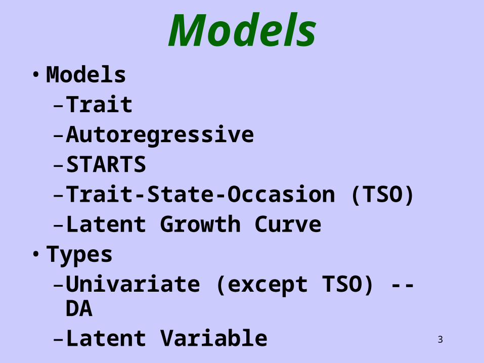
Models• Models

– Trait– Autoregressive– STARTS– Trait-State-Occasion (TSO)– Latent Growth Curve

• Types– Univariate (except TSO) -- DA– Latent Variable

4

Latent Variable Measurement Models

• Unconstrained– 2(74) = 107.71, p = .006– RMSEA = 0.032; TLI = .986

• Equal Loadings– 2(83) = 123.66, p = .003– RMSEA = 0.034; TLI = .986• The equal loading model has reasonable

fit.• All latent variable models (except

growth curve) are compared to this model.

5

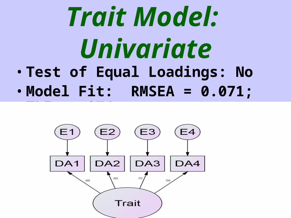
Trait Model: Univariate

• Test of Equal Loadings: No• Model Fit: RMSEA = 0.071; TLI = .974

6

Trait Model: Latent Variables

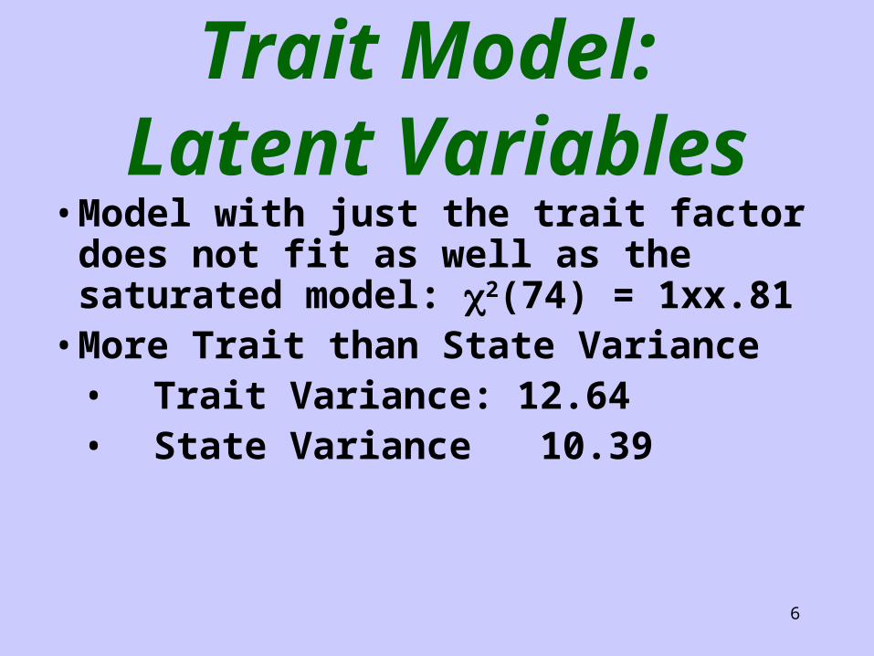
• Model with just the trait factor does not fit as well as the saturated model: 2(74) = 1xx.81

• More Trait than State Variance• Trait Variance: 12.64• State Variance 10.39

7

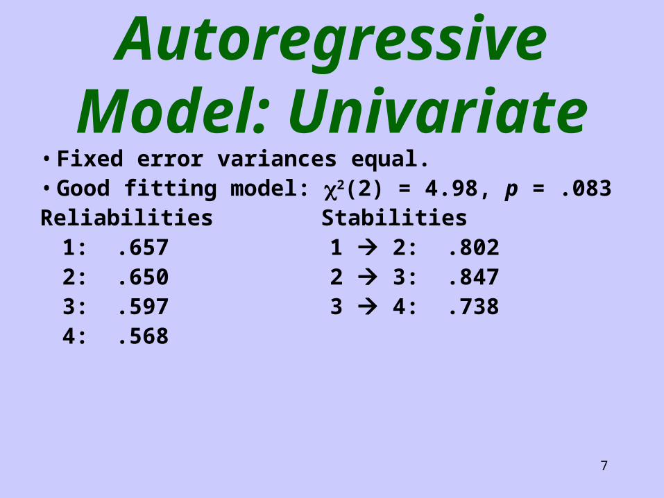
Autoregressive Model: Univariate

• Fixed error variances equal.• Good fitting model: 2(2) = 4.98, p = .083Reliabilities Stabilities

1: .657 1 2: .802 2: .650 2 3: .8473: .597 3 4: .7384: .568

8

Autoregressive Model: Latent Variables

• Not a very good fitting model compared to the CFA– 2(3) = 60.08, p < .001• Overall Fit: 2(xx) = 1.81, p < .0xx, RMSEA = 0.0xx; TLI

= .9xx• Stabilities

1 2: .xxx 2 3: .xxx3 4: .xxx

9

Growth Curve Model: Univariate

• Unlike other models it fits the means.• Fit: 2(74) = 1xx.81, p < .0xx, RMSEA = 0.0xx; TLI

= .9xx

Intercept SlopeMeanVariance

10

Growth Curve Model: Latent

VariablesFit: 2(74) = 1xx.81, p < .0xx, RMSEA = 0.0xx; TLI = .9xx

Intercept SlopeMeanVariance

11

Trait State Occasion Model

• Standard TSO does not have correlated errors, but they are added.

• Fit: 2(74) = 1xx.81, p < .0xx, RMSEA = 0.0xx; TLI = .9xx– Variances– Trait– State

12

13

STARTS Univariate

• Difficulty in finding trait factor. None of the models converged.

• Trait factor as Seasonality: Loadings in the Fall are 1 and in the Spring are -1

• Models converged.

14

Univariate STARTS Results

• Fit: 2(74) = 1xx.81, p < .0xx, RMSEA = 0.0xx; TLI = .9xx

• Variances– Seasonality – ART– State

• AR coefficient:

15

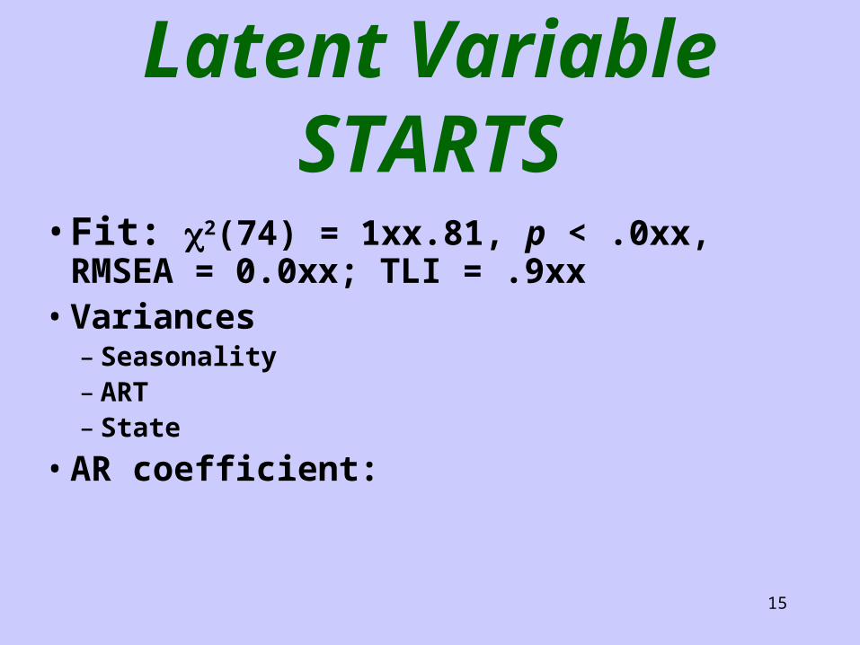
Latent Variable STARTS

• Fit: 2(74) = 1xx.81, p < .0xx, RMSEA = 0.0xx; TLI = .9xx

• Variances– Seasonality – ART– State

• AR coefficient:

16

Summary of Fit: Univariate

• Trait• Autoregressive• Growth Curve• STARTS

17

Summary of Fit: Latent Variables

RMSEA TLINo Model 0.034 .986TraitAutoregressiveGrowth CurveTSOSTARTS