Embed Size (px)
Citation preview
April 2004
EXAMPLE EXPOSURE SCENARIOS
National Center for Environmental Assessment U.S. Environmental Protection Agency
Washington, DC 20460
DISCLAIMER
This final document has been reviewed in accordance with U.S. Environmental Protection Agency policy and approved for publication. Mention of trade names or commercial products does not constitute endorsement or recommendation for use.
ABSTRACT
Exposure scenarios are a tool to help the assessor develop estimates of exposure, dose, and risk. An exposure scenario generally includes facts, data, assumptions, inferences, and sometimes professional judgment about how the exposure takes place. The human physiological and behavioral data necessary to construct exposure scenarios can be obtained from the Exposure Factors Handbook (U.S. EPA, 1997a). The handbook provides data on drinking water consumption, soil ingestion, inhalation rates, dermal factors including skin area and soil adherence factors, consumption of fruits and vegetables, fish, meats, dairy products, homegrown foods, breast milk, activity patterns, body weight, consumer products, and life expectancy.
The purpose of the Example Exposure Scenarios is to outline scenarios for various exposure pathways and to demonstrate how data from the Exposure Factors Handbook (U.S. EPA, 1997a) may be applied for estimating exposures. The example scenarios presented here have been selected to best demonstrate the use of the various key data sets in the Exposure Factors Handbook (U.S. EPA, 1997a), and represent commonly encountered exposure pathways. An exhaustive review of every possible exposure scenario for every possible receptor population would not be feasible and is not provided. Instead, readers may use the representative examples provided here to formulate scenarios that are appropriate to the assessment of interest, and apply the same or similar data sets and approaches as shown in the examples.
Preferred Citation: U.S. Environmental Protection Agency (EPA). (2003) Example Exposure Scenarios. National Center for Environmental Assessment, Washington, DC; EPA/600/R-03/036. Available from: National Information Service, Springfield, VA; PB2003-103280 and at http://www.epa.gov/ncea
i
TABLE OF CONTENTS
1.0 INTRODUCTION AND PURPOSE OF THIS DOCUMENT . . . . . . . . . . . . . . . . . . . . . 11.1 CONDUCTING AN EXPOSURE ASSESSMENT . . . . . . . . . . . . . . . . . . . . . . . 1
1.1.1 General Principles . . . . . . . . . . . . . . . . . . . . . . . . . . . . . . . . . . . . . . . . . . . 11.1.2 Important Considerations in Calculating Dose . . . . . . . . . . . . . . . . . . . . . 51.1.3 Other Sources of Information on Exposure Assessment . . . . . . . . . . . . . . 7
1.2 CHOICE OF EXPOSURE SCENARIOS . . . . . . . . . . . . . . . . . . . . . . . . . . . . . . . 81.3 CONVERSION FACTORS . . . . . . . . . . . . . . . . . . . . . . . . . . . . . . . . . . . . . . . . . 10 1.4 DEFINITIONS . . . . . . . . . . . . . . . . . . . . . . . . . . . . . . . . . . . . . . . . . . . . . . . . . . . 13
2.0 EXAMPLE INGESTION EXPOSURE SCENARIOS . . . . . . . . . . . . . . . . . . . . . . . . . . 18 2.1 PER CAPITA INGESTION OF CONTAMINATED HOMEGROWN
VEGETABLES: GENERAL POPULATION (ADULTS), CENTRALTENDENCY, LIFETIME AVERAGE EXPOSURE . . . . . . . . . . . . . . . . . . . . . 18 2.1.1 Introduction . . . . . . . . . . . . . . . . . . . . . . . . . . . . . . . . . . . . . . . . . . . . . . . 18 2.1.2 Exposure Algorithm . . . . . . . . . . . . . . . . . . . . . . . . . . . . . . . . . . . . . . . . . 18 2.1.3 Exposure Factor Inputs . . . . . . . . . . . . . . . . . . . . . . . . . . . . . . . . . . . . . . 19 2.1.4 Calculations . . . . . . . . . . . . . . . . . . . . . . . . . . . . . . . . . . . . . . . . . . . . . . . 21 2.1.5 Exposure Characterization and Uncertainties . . . . . . . . . . . . . . . . . . . . . 21
2.2 CONSUMER ONLY INGESTION OF CONTAMINATED HOMEGROWNTOMATOES: CHILDREN, HIGH-END, CHRONIC DAILY EXPOSURE . . 242.2.1 Introduction . . . . . . . . . . . . . . . . . . . . . . . . . . . . . . . . . . . . . . . . . . . . . . . 24 2.2.2 Exposure Algorithm . . . . . . . . . . . . . . . . . . . . . . . . . . . . . . . . . . . . . . . . . 24 2.2.3 Exposure Factor Inputs . . . . . . . . . . . . . . . . . . . . . . . . . . . . . . . . . . . . . . 25 2.2.4 Calculations . . . . . . . . . . . . . . . . . . . . . . . . . . . . . . . . . . . . . . . . . . . . . . . 26 2.2.5 Exposure Characterization and Uncertainties . . . . . . . . . . . . . . . . . . . . . 27
2.3 PER CAPITA INGESTION OF CONTAMINATED BEEF: ADULTS, CENTRAL TENDENCY, LIFETIME AVERAGE EXPOSURE . . . . . . . . . . . 29 2.3.1 Introduction . . . . . . . . . . . . . . . . . . . . . . . . . . . . . . . . . . . . . . . . . . . . . . . 29 2.3.2 Exposure Algorithm . . . . . . . . . . . . . . . . . . . . . . . . . . . . . . . . . . . . . . . . . 29 2.3.3 Exposure Factor Inputs . . . . . . . . . . . . . . . . . . . . . . . . . . . . . . . . . . . . . . 30 2.3.4 Calculations . . . . . . . . . . . . . . . . . . . . . . . . . . . . . . . . . . . . . . . . . . . . . . . 32 2.3.5 Exposure Characterization and Uncertainties . . . . . . . . . . . . . . . . . . . . . 32
2.4 CONSUMER ONLY INGESTION OF CONTAMINATED DAIRYPRODUCTS: GENERAL POPULATION (ALL AGES COMBINED),BOUNDING, ACUTE EXPOSURE . . . . . . . . . . . . . . . . . . . . . . . . . . . . . . . . . 34 2.4.1 Introduction . . . . . . . . . . . . . . . . . . . . . . . . . . . . . . . . . . . . . . . . . . . . . . . 34 2.4.2 Exposure Algorithm . . . . . . . . . . . . . . . . . . . . . . . . . . . . . . . . . . . . . . . . . 34 2.4.3 Exposure Factor Inputs . . . . . . . . . . . . . . . . . . . . . . . . . . . . . . . . . . . . . . 34 2.4.4 Calculations . . . . . . . . . . . . . . . . . . . . . . . . . . . . . . . . . . . . . . . . . . . . . . . 36 2.4.5 Exposure Characterization and Uncertainties . . . . . . . . . . . . . . . . . . . . . 37
ii

2.5 INGESTION OF CONTAMINATED DRINKING WATER: OCCUPATIONALADULTS, BASED ON OCCUPATIONAL TENURE, HIGH-END, LIFETIMEAVERAGE EXPOSURE . . . . . . . . . . . . . . . . . . . . . . . . . . . . . . . . . . . . . . . . . . . 38 2.5.1 Introduction . . . . . . . . . . . . . . . . . . . . . . . . . . . . . . . . . . . . . . . . . . . . . . . 38 2.5.2 Exposure Algorithm . . . . . . . . . . . . . . . . . . . . . . . . . . . . . . . . . . . . . . . . . 38 2.5.3 Exposure Factor Inputs . . . . . . . . . . . . . . . . . . . . . . . . . . . . . . . . . . . . . . 38 2.5.4 Calculations . . . . . . . . . . . . . . . . . . . . . . . . . . . . . . . . . . . . . . . . . . . . . . . 40 2.5.5 Exposure Characterization and Uncertainties . . . . . . . . . . . . . . . . . . . . . 40
2.6 INGESTION OF CONTAMINATED DRINKING WATER: SCHOOLCHILDREN, CENTRAL TENDENCY, SUBCHRONIC EXPOSURE . . . . . . . 42 2.6.1 Introduction . . . . . . . . . . . . . . . . . . . . . . . . . . . . . . . . . . . . . . . . . . . . . . . 42 2.6.2 Exposure Algorithm . . . . . . . . . . . . . . . . . . . . . . . . . . . . . . . . . . . . . . . . . 42 2.6.3 Exposure Factor Inputs . . . . . . . . . . . . . . . . . . . . . . . . . . . . . . . . . . . . . . 43 2.6.4 Calculations . . . . . . . . . . . . . . . . . . . . . . . . . . . . . . . . . . . . . . . . . . . . . . . 44 2.6.5 Exposure Characterization and Uncertainties . . . . . . . . . . . . . . . . . . . . . 44
2.7 INGESTION OF CONTAMINATED DRINKING WATER: ADULT MALES INHIGH PHYSICAL ACTIVITY OCCUPATIONS, BOUNDING, AVERAGELIFETIME EXPOSURE . . . . . . . . . . . . . . . . . . . . . . . . . . . . . . . . . . . . . . . . . . . 46 2.7.1 Introduction . . . . . . . . . . . . . . . . . . . . . . . . . . . . . . . . . . . . . . . . . . . . . . . 46 2.7.2 Exposure Algorithm . . . . . . . . . . . . . . . . . . . . . . . . . . . . . . . . . . . . . . . . . 46 2.7.3 Exposure Factor Inputs . . . . . . . . . . . . . . . . . . . . . . . . . . . . . . . . . . . . . . 47 2.7.4 Calculations . . . . . . . . . . . . . . . . . . . . . . . . . . . . . . . . . . . . . . . . . . . . . . . 48 2.7.5 Exposure Characterization and Uncertainties . . . . . . . . . . . . . . . . . . . . . 48
2.8 INCIDENTAL INGESTION OF POOL WATER: CHILDREN, BOUNDING,ACUTE EXPOSURE . . . . . . . . . . . . . . . . . . . . . . . . . . . . . . . . . . . . . . . . . . . . . . 50 2.8.1 Introduction . . . . . . . . . . . . . . . . . . . . . . . . . . . . . . . . . . . . . . . . . . . . . . . 50 2.8.2 Exposure Algorithm . . . . . . . . . . . . . . . . . . . . . . . . . . . . . . . . . . . . . . . . . 50 2.8.3 Exposure Factor Inputs . . . . . . . . . . . . . . . . . . . . . . . . . . . . . . . . . . . . . . 51 2.8.4 Calculations . . . . . . . . . . . . . . . . . . . . . . . . . . . . . . . . . . . . . . . . . . . . . . . 52 2.8.5 Exposure Characterization and Uncertainties . . . . . . . . . . . . . . . . . . . . . 52
2.9 INGESTION OF CONTAMINATED FRESHWATER AND MARINE FISH:CHILDREN, CENTRAL TENDENCY, CHRONIC EXPOSURE . . . . . . . . . . . 54 2.9.1 Introduction . . . . . . . . . . . . . . . . . . . . . . . . . . . . . . . . . . . . . . . . . . . . . . . 54 2.9.2 Exposure Algorithm . . . . . . . . . . . . . . . . . . . . . . . . . . . . . . . . . . . . . . . . . 54 2.9.3 Exposure Factor Inputs . . . . . . . . . . . . . . . . . . . . . . . . . . . . . . . . . . . . . . 55 2.9.4 Calculations . . . . . . . . . . . . . . . . . . . . . . . . . . . . . . . . . . . . . . . . . . . . . . . 57 2.9.5 Exposure Characterization and Uncertainties . . . . . . . . . . . . . . . . . . . . . 58
2.10 INGESTION OF CONTAMINATED FISH: SUBSISTENCE FISHING NATIVEAMERICAN ADULTS, BOUNDING, AVERAGE LIFETIME EXPOSURE . . 602.10.1 Introduction . . . . . . . . . . . . . . . . . . . . . . . . . . . . . . . . . . . . . . . . . . . . . . . 60 2.10.2 Exposure Algorithm . . . . . . . . . . . . . . . . . . . . . . . . . . . . . . . . . . . . . . . . . 60 2.10.3 Exposure Factor Inputs . . . . . . . . . . . . . . . . . . . . . . . . . . . . . . . . . . . . . . 61 2.10.4 Calculations . . . . . . . . . . . . . . . . . . . . . . . . . . . . . . . . . . . . . . . . . . . . . . . 62
iii

2.10.5 Exposure Characterization and Uncertainties . . . . . . . . . . . . . . . . . . . . . 62 2.11 CONSUMER ONLY INGESTION OF CONTAMINATED FISH: GENERAL
POPULATION ADULTS, HIGH-END, ACUTE EXPOSURE . . . . . . . . . . . . . 64 2.11.1 Introduction . . . . . . . . . . . . . . . . . . . . . . . . . . . . . . . . . . . . . . . . . . . . . . . 64 2.11.2 Exposure Algorithm . . . . . . . . . . . . . . . . . . . . . . . . . . . . . . . . . . . . . . . . . 64 2.11.3 Exposure Factor Inputs . . . . . . . . . . . . . . . . . . . . . . . . . . . . . . . . . . . . . . 65 2.11.4 Calculations . . . . . . . . . . . . . . . . . . . . . . . . . . . . . . . . . . . . . . . . . . . . . . . 66 2.11.5 Exposure Characterization and Uncertainties . . . . . . . . . . . . . . . . . . . . . 66
2.12 INGESTION OF CONTAMINATED BREAST MILK: INFANTS, CENTRALTENDENCY SUBCHRONIC EXPOSURE . . . . . . . . . . . . . . . . . . . . . . . . . . . . 68 2.12.1 Introduction . . . . . . . . . . . . . . . . . . . . . . . . . . . . . . . . . . . . . . . . . . . . . . . 68 2.12.2 Exposure Algorithm . . . . . . . . . . . . . . . . . . . . . . . . . . . . . . . . . . . . . . . . . 68 2.12.3 Exposure Factor Inputs . . . . . . . . . . . . . . . . . . . . . . . . . . . . . . . . . . . . . . 69 2.12.4 Calculations . . . . . . . . . . . . . . . . . . . . . . . . . . . . . . . . . . . . . . . . . . . . . . . 70 2.12.5 Exposure Characterization and Uncertainties . . . . . . . . . . . . . . . . . . . . . 71
2.13 INGESTION OF CONTAMINATED INDOOR DUST: YOUNG CHILDREN,HIGH-END, AVERAGE LIFETIME EXPOSURE . . . . . . . . . . . . . . . . . . . . . . 73 2.13.1 Introduction . . . . . . . . . . . . . . . . . . . . . . . . . . . . . . . . . . . . . . . . . . . . . . . 73 2.13.2 Exposure Algorithm . . . . . . . . . . . . . . . . . . . . . . . . . . . . . . . . . . . . . . . . . 73 2.13.3 Exposure Factor Inputs . . . . . . . . . . . . . . . . . . . . . . . . . . . . . . . . . . . . . . 74 2.13.4 Calculations . . . . . . . . . . . . . . . . . . . . . . . . . . . . . . . . . . . . . . . . . . . . . . . 75 2.13.5 Exposure Characterization and Uncertainties . . . . . . . . . . . . . . . . . . . . . 75
2.14 INGESTION OF INDOOR DUST ORIGINATING FROM OUTDOOR SOIL:OCCUPATIONAL ADULTS, CENTRAL TENDENCY, AVERAGE LIFETIMEEXPOSURE . . . . . . . . . . . . . . . . . . . . . . . . . . . . . . . . . . . . . . . . . . . . . . . . . . . . . 77 2.14.1 Introduction . . . . . . . . . . . . . . . . . . . . . . . . . . . . . . . . . . . . . . . . . . . . . . . 77 2.14.2 Exposure Algorithm . . . . . . . . . . . . . . . . . . . . . . . . . . . . . . . . . . . . . . . . . 77 2.14.3 Exposure Factor Inputs . . . . . . . . . . . . . . . . . . . . . . . . . . . . . . . . . . . . . . 78 2.14.4 Calculations . . . . . . . . . . . . . . . . . . . . . . . . . . . . . . . . . . . . . . . . . . . . . . . 79 2.14.5 Exposure Characterization and Uncertainties . . . . . . . . . . . . . . . . . . . . . 79
3.0 EXAMPLE INHALATION EXPOSURE SCENARIOS . . . . . . . . . . . . . . . . . . . . . . . . 81 3.1 INHALATION OF CONTAMINATED INDOOR AIR: OCCUPATIONAL
FEMALE ADULTS, CENTRAL TENDENCY, AVERAGE LIFETIMEEXPOSURE . . . . . . . . . . . . . . . . . . . . . . . . . . . . . . . . . . . . . . . . . . . . . . . . . . . . . 82 3.1.1 Introduction . . . . . . . . . . . . . . . . . . . . . . . . . . . . . . . . . . . . . . . . . . . . . . . 82 3.1.2 Exposure Algorithm . . . . . . . . . . . . . . . . . . . . . . . . . . . . . . . . . . . . . . . . . 82 3.1.4 Calculations . . . . . . . . . . . . . . . . . . . . . . . . . . . . . . . . . . . . . . . . . . . . . . . 83 3.1.5 Exposure Characterization and Uncertainties . . . . . . . . . . . . . . . . . . . . . 84
3.2 INHALATION OF CONTAMINATED INDOOR AIR: RESIDENTIAL CHILD,CENTRAL TENDENCY, AVERAGE LIFETIME EXPOSURE . . . . . . . . . . . . 85 3.2.1 Introduction . . . . . . . . . . . . . . . . . . . . . . . . . . . . . . . . . . . . . . . . . . . . . . . 85 3.2.2 Exposure Algorithm . . . . . . . . . . . . . . . . . . . . . . . . . . . . . . . . . . . . . . . . . 85
iv

3.2.3 Exposure Factor Inputs . . . . . . . . . . . . . . . . . . . . . . . . . . . . . . . . . . . . . . 85 3.2.4 Calculations . . . . . . . . . . . . . . . . . . . . . . . . . . . . . . . . . . . . . . . . . . . . . . . 86 3.2.5 Exposure Characterization and Uncertainties . . . . . . . . . . . . . . . . . . . . . 87
3.3 INHALATION OF CONTAMINATED INDOOR AIR: SCHOOL CHILDREN,CENTRAL TENDENCY, SUBCHRONIC EXPOSURE . . . . . . . . . . . . . . . . . . 88 3.3.1 Introduction . . . . . . . . . . . . . . . . . . . . . . . . . . . . . . . . . . . . . . . . . . . . . . . 88 3.3.2 Exposure Algorithm . . . . . . . . . . . . . . . . . . . . . . . . . . . . . . . . . . . . . . . . . 88 3.3.3 Exposure Factor Inputs . . . . . . . . . . . . . . . . . . . . . . . . . . . . . . . . . . . . . . 88 3.3.4 Calculations . . . . . . . . . . . . . . . . . . . . . . . . . . . . . . . . . . . . . . . . . . . . . . . 89 3.3.5 Exposure Characterization and Uncertainties . . . . . . . . . . . . . . . . . . . . . 90
4.0 EXAMPLE DERMAL EXPOSURE SCENARIOS . . . . . . . . . . . . . . . . . . . . . . . . . . . . 91 4.1 DERMAL CONTACT WITH CONTAMINATED SOIL: RESIDENTIAL
ADULT GARDENERS, CENTRAL TENDENCY, AVERAGE LIFETIME EXPOSURE. . . . . . . . . . . . . . . . . . . . . . . . . . . . . . . . . . . . . . . . . . . . . . . . . . . . . . . . . . . . . . . 91
4.1.1 Introduction . . . . . . . . . . . . . . . . . . . . . . . . . . . . . . . . . . . . . . . . . . . . . . . 91 4.1.2 Exposure Algorithm . . . . . . . . . . . . . . . . . . . . . . . . . . . . . . . . . . . . . . . . . 91 4.1.3 Exposure Factor Inputs . . . . . . . . . . . . . . . . . . . . . . . . . . . . . . . . . . . . . . 92 4.1.4 Calculations . . . . . . . . . . . . . . . . . . . . . . . . . . . . . . . . . . . . . . . . . . . . . . . 96 4.1.5 Exposure Characterization and Uncertainties . . . . . . . . . . . . . . . . . . . . . 98
4.2 DERMAL CONTACT WITH SOIL: TEEN ATHLETE: CENTRALTENDENCY, SUBCHRONIC EXPOSURE . . . . . . . . . . . . . . . . . . . . . . . . . . . 100 4.2.1 Introduction . . . . . . . . . . . . . . . . . . . . . . . . . . . . . . . . . . . . . . . . . . . . . . 100 4.2.2 Exposure Algorithm . . . . . . . . . . . . . . . . . . . . . . . . . . . . . . . . . . . . . . . . 100 4.2.3 Exposure Factor Inputs . . . . . . . . . . . . . . . . . . . . . . . . . . . . . . . . . . . . . 101 4.2.4 Calculations . . . . . . . . . . . . . . . . . . . . . . . . . . . . . . . . . . . . . . . . . . . . . . 105 4.2.5 Exposure Characterization and Uncertainties . . . . . . . . . . . . . . . . . . . . 106
4.3 DERMAL CONTACT WITH CONSUMER PRODUCTS: GENERALPOPULATION ADULTS, CENTRAL TENDENCY, AVERAGE LIFETIMEEXPOSURE . . . . . . . . . . . . . . . . . . . . . . . . . . . . . . . . . . . . . . . . . . . . . . . . . . . . 108 4.3.1 Introduction . . . . . . . . . . . . . . . . . . . . . . . . . . . . . . . . . . . . . . . . . . . . . . 108 4.3.2 Exposure Algorithm . . . . . . . . . . . . . . . . . . . . . . . . . . . . . . . . . . . . . . . . 108 4.3.3 Exposure Factor Inputs . . . . . . . . . . . . . . . . . . . . . . . . . . . . . . . . . . . . . 109 4.3.4 Calculations . . . . . . . . . . . . . . . . . . . . . . . . . . . . . . . . . . . . . . . . . . . . . . 111 4.3.5 Exposure Characterization and Uncertainties . . . . . . . . . . . . . . . . . . . . 112
4.4 DERMAL CONTACT WITH SURFACE WATER: RECREATIONALCHILDREN, CENTRAL TENDENCY, AVERAGE LIFETIME EXPOSURE
. . . . . . . . . . . . . . . . . . . . . . . . . . . . . . . . . . . . . . . . . . . . . . . . . . . . . . . . . . . . . . 113 4.4.1 Introduction . . . . . . . . . . . . . . . . . . . . . . . . . . . . . . . . . . . . . . . . . . . . . . 113 4.4.2 Exposure Algorithm . . . . . . . . . . . . . . . . . . . . . . . . . . . . . . . . . . . . . . . . 113 4.4.3 Exposure Factor Inputs . . . . . . . . . . . . . . . . . . . . . . . . . . . . . . . . . . . . . 114 4.4.4 Calculations . . . . . . . . . . . . . . . . . . . . . . . . . . . . . . . . . . . . . . . . . . . . . . 119 4.4.5 Exposure Characterization and Uncertainties . . . . . . . . . . . . . . . . . . . . 120
v

5.0 REFERENCES . . . . . . . . . . . . . . . . . . . . . . . . . . . . . . . . . . . . . . . . . . . . . . . . . . . . . . . 121
vi

LIST OF TABLES
Table 1. Roadmap of Example Exposure Scenarios Conversion Factors . . . . . . . . . . . . . . . . . . 11
Table 2. Conversion Factors . . . . . . . . . . . . . . . . . . . . . . . . . . . . . . . . . . . . . . . . . . . . . . . . . . . . 12
Table 3. Homegrown Vegetable Intake Rates . . . . . . . . . . . . . . . . . . . . . . . . . . . . . . . . . . . . . . . 20
Table 4. Homegrown Tomato Intake Rate . . . . . . . . . . . . . . . . . . . . . . . . . . . . . . . . . . . . . . . . . 25
Table 5. Percentage Lipid Content of Beef . . . . . . . . . . . . . . . . . . . . . . . . . . . . . . . . . . . . . . . . . 30
Table 6. Adult Beef Intake Rates . . . . . . . . . . . . . . . . . . . . . . . . . . . . . . . . . . . . . . . . . . . . . . . . 31
Table 7. Weighted Average Body Weight (Ages 1-75) . . . . . . . . . . . . . . . . . . . . . . . . . . . . . . . 36
Table 8. Drinking Water Intake Rate for School Children (Ages 4-10) . . . . . . . . . . . . . . . . . . . 43
Table 9. Marine and Freshwater Intake Rates . . . . . . . . . . . . . . . . . . . . . . . . . . . . . . . . . . . . . . . 56
Table 10. Average Body Weight For Children, Age 2-9 . . . . . . . . . . . . . . . . . . . . . . . . . . . . . . 57
Table 11. Male and Female Intake Rates for Fish . . . . . . . . . . . . . . . . . . . . . . . . . . . . . . . . . . . 65
Table 12. Breast Milk Intake Rates . . . . . . . . . . . . . . . . . . . . . . . . . . . . . . . . . . . . . . . . . . . . . . . 70
Table 13. Body Surface Areas for Residential Gardeners . . . . . . . . . . . . . . . . . . . . . . . . . . . . . 94
Table 14. Soil Adherence For Residential Gardeners . . . . . . . . . . . . . . . . . . . . . . . . . . . . . . . . . 95
Table 15. Surface Area For Teen Athletes . . . . . . . . . . . . . . . . . . . . . . . . . . . . . . . . . . . . . . . . 102
Table 16. Soil Adherence For Teen Athletes . . . . . . . . . . . . . . . . . . . . . . . . . . . . . . . . . . . . . . 103
Table 17. Body Part Percentages . . . . . . . . . . . . . . . . . . . . . . . . . . . . . . . . . . . . . . . . . . . . . . . 110
Table 18. Surface Area for Children, Age 7-12 Years . . . . . . . . . . . . . . . . . . . . . . . . . . . . . . . 117
Table 19. Body Surface Area Exposed During Wading . . . . . . . . . . . . . . . . . . . . . . . . . . . . . . 118
vii
PREFACE
The National Center for Environmental Assessment (NCEA) of EPA’s Office of Research and Development prepared the Example Exposure Scenarios to outline scenarios for various exposure pathways and to demonstrate how data from the Exposure Factors Handbook (U.S. EPA, 1997a) may be applied for estimating exposures. The Example Exposure Scenarios is intended to be a companion document to the Exposure Factors Handbook. The example scenarios presented were compiled from questions and inquiries received from users of the Exposure Factors Handbook during the past few years on how to select data from the Handbook. Although a few children scenarios are included in this report, a separate and more comprehensive document specifically focusing on children scenarios is planned as soon as the Child-Specific Exposure Factors Handbook is finalized.
The scenarios examined in this report refer to a single chemical and exposure route. However, EPA promotes and supports the use of new and innovative approaches and tools to improve the quality of public health and environmental protection. For example, characterizing the exposures to an individual throughout the different life stages is an area of growing interest. In addition, in the past few years there has been an increased emphasis in cumulative risk assessments1, aggregate exposures2, and chemical mixtures. Detailed and comprehensive guidance for evaluating cumulative risk is not currently available. The Agency has, however, developed a framework that lays out a broad outline of the assessment process and provides a basic structure for evaluating cumulative risks. This basic structure is presented in the Framework for Cumulative Risk Assessment published in May 2003 (U.S. EPA 2003).
The Example Exposure Scenarios does not include an example of a probabilistic assessment. However, the use of probabilistic methods to characterize the degree of variability and/or uncertainty in risk estimates is a tool of growing demand. In contrast to the point-estimate approach, probabilistic methods allow for a better characterization of variability and/or uncertainty in risk estimates. These techniques are increasingly being used to quantify the range and likelihood of possible exposure outcomes. Various Program Offices in EPA are directing efforts to develop guidance on the use of probabilistic techniques. Some of these efforts include:
• Summary Report for the Workshop on the Monte Carlo Analysis. U.S. EPA 1996 • Guiding Principles for Monte Carlo Analysis. U.S. EPA 1997b
http://www.epa.gov/ncea/raf/montecar.pdf • Policy for Use of Probabilistic Analysis in Risk Assessment, U.S. 1997c
1 Cumulative risk assessment - An analysis, characterization, and possible quantification of the combined risks to health or the environment from multiple agents or stressors.
2 Aggregate exposures - The combined exposure of an individual (or defined population) to a specific agent or stressor via relevant routes, pathways, and sources.
viii

• Guidance for Submission of Probabilistic Exposure Assessments to the Office of Pesticide Programs’Health Effects Division -Draft, U.S.EPA 1998a http://www.epa.gov/oscpmont/sap/1998/march/backgrd.pdf
• Report of the Workshop on Selecting Input Distributions for Probabilistic Assessments. U.S. EPA 1999
• Options for Development of Parametric Probability Distributions for Exposure Factors. U.S. EPA 2000a
• Risk Assessment Guidance for Superfund: Volume III - Part A, Process for Conducting Probabilistic Assessment, U.S. EPA 2001a http://www.epa.gov/superfund/programs/risk/rags3a/index.htm
In general, the Agency advocates a tiered approach, which begins with a point estimate risk assessment. Further refinements to the assessment may be conducted after studying several important considerations, such as resources, quality and quantity of exposure data available, and value added by conducting a probabilistic assessment (U.S. EPA 2001a). Great attention needs to be placed in the development of distributions and how they influence the results. A more extensive discussion of these techniques can be found in EPA 2001a.
ix

AUTHORS, CONTRIBUTORS, AND REVIEWERS
The National Center for Environmental Assessment (NCEA), Office of Research and Development was responsible for the preparation of this document. This document has been prepared by the Exposure Assessment Division of Versar Inc. in Springfield, Virginia, under EPA Contract No. 68-W-99-041. Jacqueline Moya served as Work Assignment Manager, providing overall direction, technical assistance, and serving as contributing author.
AUTHORS WORD PROCESSING
Versar, Inc. Versar, Inc. Linda Phillips Valerie Schwartz
Wendy Powell
CONTRIBUTORS TECHNICAL EDITING
Versar U.S. EPA Nathan Mottl Laurie Schuda Kelly McAloon C. William Smith
U.S. EPA Jacqueline Moya Laurie Schuda
The following EPA individuals reviewed an earlier draft of this document and provided valuable comments:
Marcia Bailey, U.S. EPA, Region X Denis R. Borum, U.S. EPA, Office of Water, Health and Ecological Criteria Division Pat Kennedy, U.S. EPA, Office of Prevention, Pesticides, and Toxic Substances Youngmoo Kim, U.S. EPA, Region VI Lon Kissinger, U.S. EPA, Region X Roseanne Lorenzana, U.S. EPA, Region X Tom McCurdy, U.S. EPA, Office of Research and Development, National Exposure Research
Laboratory Debdas Mukerjee, U.S. EPA, Office of Research and Development, National Center for
Environmental Assessment-Cincinnatti Marian Olsen, U.S. EPA, Region II Marc Stifelman, U.S. EPA, Region X
x

This document was reviewed by an external panel of experts. The panel was composed of the following individuals:
Dr. Robert Blaisdell California Environmental Protection Agency1515 Clay St., 16th FloorOakland, California 94612
Dr. Amy Arcus Arth California Environmental Protection Agency1515 Clay St., 16th FloorOakland, California 94612
Dr. Annette Guiseppi-Elie DuPont Spruance Plant5401 Jefferson Davis HighwayP.O. Box 126 Richmond, Virginia 23234
Dr. Steven D. Colome University of South Carolina School of Medicine6311 Garners Ferry Road Columbia, South Carolina 29209
Dr. Annette Bunge Colorado School of Mines1500 Illinois StGolden, Colorado 80401
Dr. Mary Kay O’Rourke The University of ArizonaTucson, Arizona 85721
xi
1.0 INTRODUCTION AND PURPOSE OF THIS DOCUMENT
The Exposure Factors Handbook was published in 1997 (U.S. EPA, 1997a; http://www.epa.gov/ncea/exposfac.htm). Its purpose is to provide exposure assessors with information on physiological and behavioral factors that may be used to assess human exposure. Exposure parameters include factors such as drinking water, food, and soil intake rates, inhalation rates, skin surface area, body weight, and exposure duration. Behavioral information (e.g., activity pattern data) is included for estimating exposure frequency and duration. The Exposure Factors Handbook (U.S. EPA, 1997a) provides recommended values for use in exposure assessment, as well as confidence ratings for the various factors. However, specific examples of how the data may be used to assess exposure are not provided.
The purpose of this document is to outline scenarios for various exposure pathways and to demonstrate how data from the Exposure Factors Handbook (U.S. EPA, 1997a) may be applied for estimating exposures. It should be noted that the example scenarios presented here have been selected to best demonstrate the use of the various key data sets in the Exposure Factors Handbook (U.S. EPA, 1997a), and represent commonly encountered exposure pathways. An exhaustive review of every possible exposure scenario for every possible receptor population would not be feasible and is not provided. Instead, readers may use the representative examples provided here to formulate scenarios that are appropriate to the assessment of interest and apply the same or similar data sets and approaches as shown in the examples.
1.1 CONDUCTING AN EXPOSURE ASSESSMENT
1.1.1 General Principles
Exposure assessment is the process by which: (1) potentially exposed populations are identified; (2) potential pathways of exposure and exposure conditions are identified; and (3) chemical intakes/potential doses are quantified. Exposure may occur by ingestion, inhalation, or dermal absorption routes. Exposure is commonly defined as contact of visible external physical boundaries (i.e., mouth, nostrils, skin) with a chemical agent (U.S. EPA, 1992a). As described in EPA’s Guidelines for Exposure Assessment (U.S. EPA, 1992a), exposure is dependent upon the intensity, frequency, and duration of contact. The intensity of contact is typically expressed in terms of the concentration of contaminant per unit mass or volume (i.e., µg/g, µg/L, mg/m3, ppm, etc.) in the media to which humans are exposed (U.S. EPA, 1992a).
1
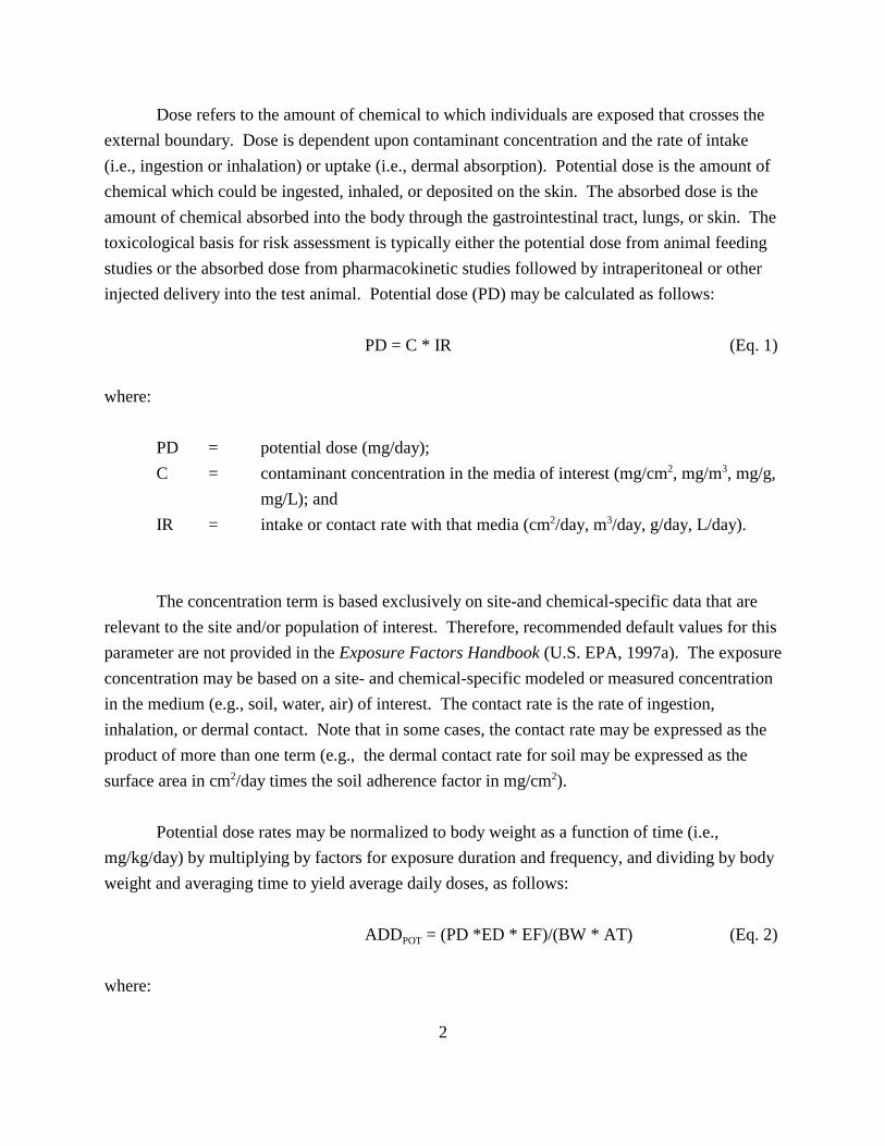
Dose refers to the amount of chemical to which individuals are exposed that crosses the external boundary. Dose is dependent upon contaminant concentration and the rate of intake (i.e., ingestion or inhalation) or uptake (i.e., dermal absorption). Potential dose is the amount of chemical which could be ingested, inhaled, or deposited on the skin. The absorbed dose is the amount of chemical absorbed into the body through the gastrointestinal tract, lungs, or skin. The toxicological basis for risk assessment is typically either the potential dose from animal feeding studies or the absorbed dose from pharmacokinetic studies followed by intraperitoneal or other injected delivery into the test animal. Potential dose (PD) may be calculated as follows:
PD = C * IR (Eq. 1)
where:
PD = potential dose (mg/day); C = contaminant concentration in the media of interest (mg/cm2, mg/m3, mg/g,
mg/L); and IR = intake or contact rate with that media (cm2/day, m3/day, g/day, L/day).
The concentration term is based exclusively on site-and chemical-specific data that are relevant to the site and/or population of interest. Therefore, recommended default values for this parameter are not provided in the Exposure Factors Handbook (U.S. EPA, 1997a). The exposure concentration may be based on a site- and chemical-specific modeled or measured concentration in the medium (e.g., soil, water, air) of interest. The contact rate is the rate of ingestion, inhalation, or dermal contact. Note that in some cases, the contact rate may be expressed as the product of more than one term (e.g., the dermal contact rate for soil may be expressed as the surface area in cm2/day times the soil adherence factor in mg/cm2).
Potential dose rates may be normalized to body weight as a function of time (i.e., mg/kg/day) by multiplying by factors for exposure duration and frequency, and dividing by body weight and averaging time to yield average daily doses, as follows:
ADDPOT = (PD *ED * EF)/(BW * AT) (Eq. 2)
where:
2
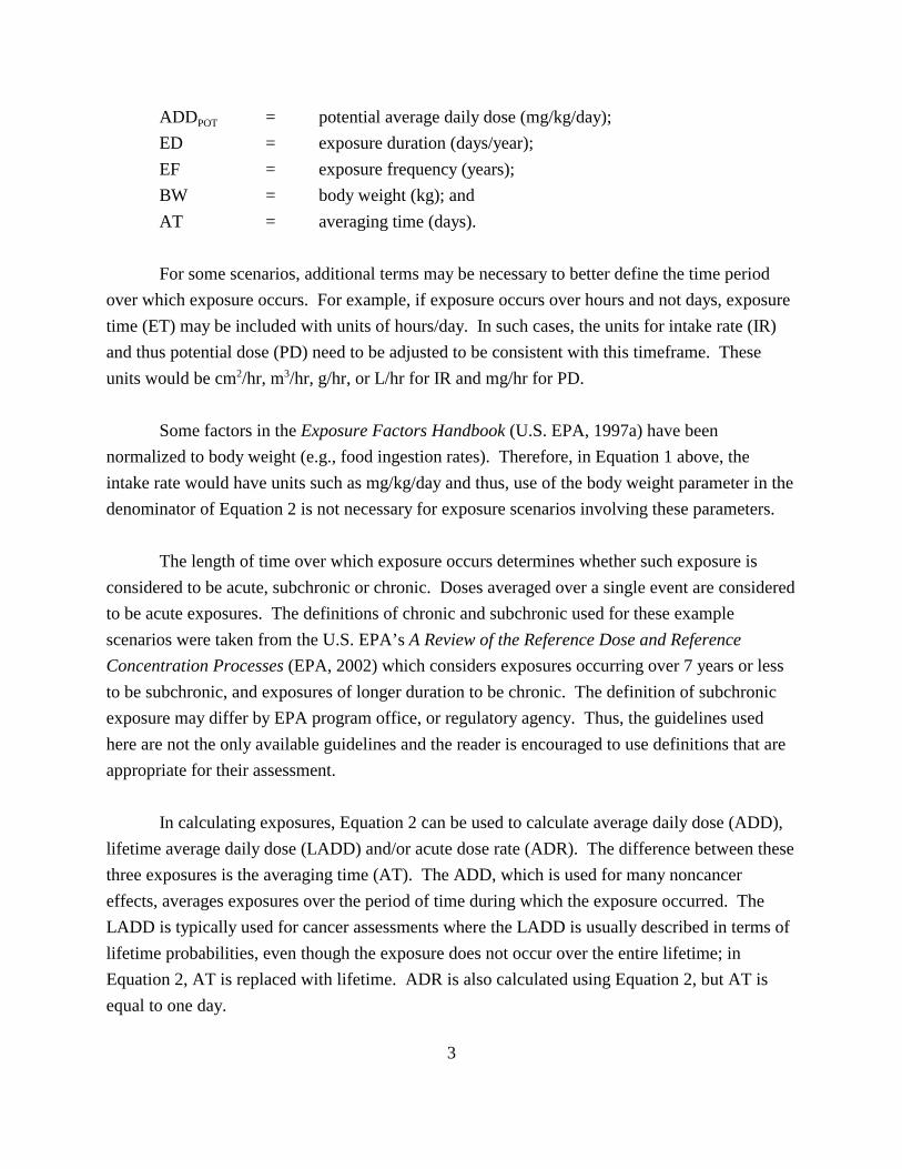
ADDPOT = potential average daily dose (mg/kg/day); ED = exposure duration (days/year); EF = exposure frequency (years); BW = body weight (kg); and AT = averaging time (days).
For some scenarios, additional terms may be necessary to better define the time period over which exposure occurs. For example, if exposure occurs over hours and not days, exposure time (ET) may be included with units of hours/day. In such cases, the units for intake rate (IR) and thus potential dose (PD) need to be adjusted to be consistent with this timeframe. These units would be cm2/hr, m3/hr, g/hr, or L/hr for IR and mg/hr for PD.
Some factors in the Exposure Factors Handbook (U.S. EPA, 1997a) have been normalized to body weight (e.g., food ingestion rates). Therefore, in Equation 1 above, the intake rate would have units such as mg/kg/day and thus, use of the body weight parameter in the denominator of Equation 2 is not necessary for exposure scenarios involving these parameters.
The length of time over which exposure occurs determines whether such exposure is considered to be acute, subchronic or chronic. Doses averaged over a single event are considered to be acute exposures. The definitions of chronic and subchronic used for these example scenarios were taken from the U.S. EPA’s A Review of the Reference Dose and Reference Concentration Processes (EPA, 2002) which considers exposures occurring over 7 years or less to be subchronic, and exposures of longer duration to be chronic. The definition of subchronic exposure may differ by EPA program office, or regulatory agency. Thus, the guidelines used here are not the only available guidelines and the reader is encouraged to use definitions that are appropriate for their assessment.
In calculating exposures, Equation 2 can be used to calculate average daily dose (ADD), lifetime average daily dose (LADD) and/or acute dose rate (ADR). The difference between these three exposures is the averaging time (AT). The ADD, which is used for many noncancer effects, averages exposures over the period of time during which the exposure occurred. The LADD is typically used for cancer assessments where the LADD is usually described in terms of lifetime probabilities, even though the exposure does not occur over the entire lifetime; in Equation 2, AT is replaced with lifetime. ADR is also calculated using Equation 2, but AT is equal to one day.
3

Absorbed doses may be calculated by including an absorption factor in the equations above. The portion of the potential dose (e.g., ADDPOT) that actually penetrates through the absorption barriers of the organism (e.g., the gut, the lung or the skin) is the absorbed dose (e.g., ADDABS) or internal dose. In this situation, the absorbed dose may be related to the potential dose through an absorption factor (ABS) as follows:
ADDABS = ADDPOT x ABS (Eq. 3)
Potential dose estimates may not be meaningful for dermal exposures to contaminants in large volumes of media (e.g., contaminated water in pools, baths and showers). For exposure scenarios of this type, absorbed dose estimates are necessary.
Central tendency, high-end, and/or bounding estimates may be made using this algorithm. These exposure descriptors account for individual and population variability and represent points on the distribution of exposures. Central tendency potential dose rates may be estimated using central tendency values for all the input values in the algorithm. The high-end potential dose rate (90th or 99.9th percentile) is a reasonable approximation of dose at the upper end of the distribution of exposures (U.S. EPA, 1992a). High-end values are estimated by setting some, but not all, input parameters to upper-end values. Finally, bounding potential dose rates are exposures that are estimated to be greater than the highest individual exposure in the population of interest. Bounding estimates use all upper-percentile inputs and are often used in screening-level assessments. (Note: users are cautioned about using all high-end inputs except in cases where screening level or acute estimates are desired because setting all exposure factor inputs to upper-percentile values may result in dose estimates that exceed reasonable maximum values for the population of interest.) Upper-percentile values are also frequently used in estimating acute exposures. For example, an assessor may wish to use a maximum value to represent the contaminant concentration in an acute exposure assessment but evaluate chronic exposures using an average (or 95% upper confidence level of the mean) contaminant concentration.
4

1.1.2 Important Considerations in Calculating Dose
Inputs for the exposure calculations shown above should be representative of the populations and pathways of exposure. It is important to select the age group, ethnic or regional population, or other population category of interest. Use of data from unrelated groups is not recommended. Frequently, exposure scenarios are developed to assist the assessor in defining the specific receptor populations and exposure conditions for which doses will be calculated. In general, an exposure scenario is defined as a set of facts, assumptions, and inferences about how exposure takes place that aids the exposure assessor in evaluating, estimating, or quantifying exposure. For the purposes of demonstrating how data from the Exposure Factors Handbook (U.S. EPA, 1997a) can be used to assess exposures, numerous example scenarios have been developed. Each scenario is explained in terms of the exposure pathway, receptor population, duration of exposure (acute, subchronic, chronic or lifetime), and exposure descriptor (i.e., central tendency, high-end, or bounding).
In addition to using exposure factor data that are specific to the population/receptor of interest, several other important issues should be considered in assessing exposure. First, it is important to ensure that the units of measure used for contact rate are consistent with those used for intake rate. Examples of where units corrections may be needed are in converting skin surface areas between units of cm2/event and m2/event to be consistent with surface residue concentrations, or converting breast milk intake rates from g/day to mL/day to be consistent with breast milk chemical concentrations. Common conversion factors are provided in Table 2 to assist the user in making appropriate conversions. Another example of where specific types of units corrections may be required is with ingestion rates. As described in Volume II of the Exposure Factors Handbook, residue concentrations in foods may be based on wet (whole) weights, lipid weights, or dry weights. The assessor must ensure that the units used for concentration are consistent with those used for ingestion rate. For example, if residue concentrations in beef are reported as mg of contaminant/g of beef fat, the intake rate for beef should be g beef fat consumed/day. This may require that the beef ingestion rate presented in units of g beef, as consumed (whole weight)/day in the Exposure Factors Handbook (U.S. EPA, 1997a) be converted to g beef fat consumed/day using the fat content of beef and the conversion equations provided in the Exposure Factors Handbook (U.S. EPA, 1997a). Alternatively, the residue concentration can be converted to units that are consistent with the intake rate units.
5

Another important consideration is the linkage between contact rate and exposure frequency. It is important to define exposure frequency so that it is consistent with the contact rate estimate. For example, the food ingestion rate can be based on a single event such as a serving size/event, or on a long-term average (e.g., daily average ingestion rate in g/day). For contact rates based on a single event, a frequency that represents the number of events over time (e.g., events/year) would be appropriate. However, when a long-term average is used, the duration over which the contact rate is based must be used. For example, when an annual daily average ingestion rate is used, 365 days/year must be used as the exposure frequency because the food intake rate represents the average daily intake over a year including both days when the food was consumed and days when the food was not consumed. The objective is to define the terms so that, when multiplied, they give the appropriate estimate of mass of contaminant contacted.
For some factors such as food, water, and soil ingestion, there is another important issue to consider. The assessor must decide whether the assessment will evaluate exposure for consumers only, or on a per capita basis. Consumer only assessments include only those individuals who are engaged in the activity of interest (e.g., fish consumption). Thus, the exposure factors (e.g., fish intake rates) are averaged over users only. In contrast, per capita data are used to assess exposure over the entire population of both users and non-users. The variability in the population should also be considered. As described above, central tendency, high-end, or bounding estimates may be generated, depending on the input factors used.
Also, as described above, for some exposure factors (e.g., intake rates for some foods), body weight has been factored into the intake rate. In these cases, the intake rates are expressed in units such as mg/kg/day. When exposure factors have been indexed to body weight, the term body weight can be eliminated from the denominator of the dose equation because body weight has already been accounted for.
Uncertainty may be introduced into the dose calculations at various stages of the exposure assessment process. Uncertainty may occur as a result of: the techniques used to estimate chemical residue concentrations (these are not addressed in the Exposure Factors Handbook (U.S. EPA, 1997a) or here), or the selection of exposure scenarios or factors. Variability can occur as a result of variations in individual day-to-day or event-to-event exposure factors or variations among the exposed population. Variability can be addressed by estimating exposure for the various descriptors of exposure (i.e., central tendency, high-end, or bounding) to estimate points on the distribution of exposure, as described above. The reader should refer to Volume I,
6

Chapter 2 of the Exposure Factors Handbook (U.S. EPA, 1997a) for a detailed discussion of variability and uncertainty. Also, as described in the Exposure Factors Handbook (U.S. EPA, 1997a), some factors have higher confidence ratings than others. These confidence ratings are based on, among other things, the representativeness, quality, and quantity of the data on which a specific recommended exposure factor is based. Assessors should consider these confidence ratings, as well as other limitations of the data in presenting a characterization of the exposure estimates generated using data from the Exposure Factors Handbook (U.S. EPA, 1997a).
1.1.3 Other Sources of Information on Exposure Assessment
For additional information on exposure assessment, the reader is encouraged to refer to the following EPA documents:
• Guidelines for Exposure Assessment (U.S. EPA 1992a;http://www.epa.gov/nceawww1/exposure.htm);
• Dermal Exposure Assessment: Principles and Applications (U.S. EPA 1992b; http://oaspub.epa.gov/eims/eimsapi.detail?deid=12188&partner=ORD-NCEA. Note that in September 2001, EPA proposed Supplemental Guidance for Dermal Risk Assessment, under Part E of Risk Assessment Guidance for Superfund (RAGS) (See below). This guidance updates many portions of this earlier 1992 guidance. Although still not final, the 2001 guidance is generally more representative of current thinking in this area and assessors are encouraged to use it instead of U.S. EPA, 1992b.);
• Methodology for Assessing Health Risks Associated with Indirect Exposure to Combustor Emissions (U.S. EPA, 1990);
• Risk assessment guidance for Superfund. Human health evaluation manual: Part A. Interim Final (U.S. EPA., 1989; http://www.epa.gov/superfund/programs/risk/ragsa/index.htm)
• Risk Assessment Guidance for Superfund. Human health evaluation manual: Part B. Interim Final (U.S. EPA., 1991; http://www.epa.gov/superfund/programs/risk/ragsb/index.htm)
• Risk Assessment Guidance for Superfund. Human health evaluation manual: Part C. Interim Final (U.S. EPA., 1991; http://www.epa.gov/superfund/programs/risk/ragsc/index.htm)
7

• Risk Assessment Guidance for Superfund. Human health evaluation manual: Part D. Interim Final (U.S. EPA., 1998b; http://www.epa.gov/superfund/programs/risk/ragsd/index.htm)
• Risk Assessment Guidance for Superfund. Human health evaluation manual: Part E. Interim Final (U.S. EPA., 2001b http://www.epa.gov/superfund/programs/risk/ragse)
• Estimating Exposures to Dioxin-Like Compounds (U.S. EPA, 1994);
• Superfund Exposure Assessment Manual (U.S. EPA, 1988a);
• Selection Criteria for Mathematical Models Used in Exposure Assessments (Surface water and Ground water) (U.S. EPA 1987 & U.S. EPA 1988b);
• Standard Scenarios for Estimating Exposure to Chemical Substances During Use of Consumer Products (U.S. EPA 1986a);
• Pesticide Assessment Guidelines, Subdivisions K and U (U.S. EPA, 1984, 1986b);
• Methods for Assessing Exposure to Chemical Substances, Volumes 1-13 (U.S. EPA, 1983-1989, available through NTIS);
• Standard Operating Procedures (SOPs) for Residential Exposure Assessments, draft (U.S. EPA, 1997d; http://www.epa.gov/oscpmont/sap/1997/september/sopindex.htm); and
• Soil Screening Guidance, Technical Background Document (U.S., EPA, 1996b, 2001; http://www.epa.gov/superfund/resources/soil/introtbd.htm).
• Revised Methodology for Deriving Health-Based Ambient Water Quality Criteria (U.S. EPA 2000b; http://www.epa.gov/waterscience/humanhealth/method/)
1.2 CHOICE OF EXPOSURE SCENARIOS
This document is not intended to be prescriptive, or inclusive of every possible exposure scenario that an assessor may want to evaluate. Instead, it is intended to provide a representative sampling of scenarios that depict use of the various data sets in the Exposure Factors Handbook (U.S. EPA, 1997a). Likewise, this document is not intended to be program-specific. Policies within different EPA program offices may vary, and the examples presented in this document are not meant to supercede program-specific exposure assessment methods or assumptions.
8

Exposure assessors are encouraged to review the examples provided here and select the examples that are most applicable to the scenarios they wish to evaluate. The approaches suggested here are not the only approaches that can be used and the data may be modified, as needed, to fit the scenario of interest. For instance, an example scenario may use ingestion of drinking water among children between the ages of 1 and 5 years to demonstrate the use of drinking water intake data, while the assessor is interested in children between the ages of 12 and 18 years. Therefore, the assessor may wish to use the suggested approach and the same data set, but use data for a different age group. Likewise, examples may depict upper bound exposures, while an assessment of central tendency is required, or chronic exposure may be shown in the example when an estimate of acute exposure is desired. Again, the suggested approach may be used with different inputs from the same or related data set. Where site-specific data are available, they may be used to replace data presented in the examples. Although calculation of health risks and the use of chemical-specific toxicity data are beyond the scope of this document, selection of input data requires consideration of the toxicity data for the chemical contaminant being assessed. For example, averaging times will vary depending on whether the contaminant is a carcinogen or not. Also, the health-based impact of an exposure may be related to life-stage because system and organ development vary with time. Thus, exposure factor data that are relevant to the activities, behaviors, and physical characteristics of the relevant age groups should be used. Other attributes of the exposed population of interest (e.g., gender, race) should also be given careful consideration when formulating an exposure scenario and selecting input data.
An effort has been made to present examples that represent a wide range of possible scenarios in terms of receptor populations, exposure descriptor (i.e., central tendency, high-end, or bounding exposure), and exposure duration (i.e., acute, subchronic, or chronic). These example scenarios utilize single values for each input parameter (i.e., point estimates), as required to conduct deterministic assessments. Probabilistic techniques are not presented. However, the same algorithms and the same data distributions from which the point estimates are derived may be used in probabilistic assessments (e.g., Monte Carlo analyses). Readers who wish to conduct probabilistic assessments should refer to Volume I, Chapter 1 of EPA’s Exposure Factors Handbook (U.S. EPA, 1997a) for general considerations for conducting such analyses. In addition, multiple pathway/source scenarios are not included in the examples presented here. These scenarios are being considered and discussed by the U.S. EPA and an agency workgroup is in the process of developing a framework for evaluating such scenarios.
9
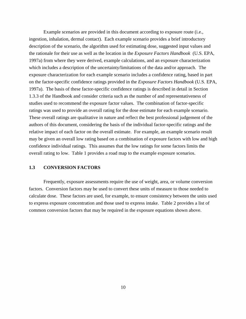
Example scenarios are provided in this document according to exposure route (i.e., ingestion, inhalation, dermal contact). Each example scenario provides a brief introductory description of the scenario, the algorithm used for estimating dose, suggested input values and the rationale for their use as well as the location in the Exposure Factors Handbook (U.S. EPA, 1997a) from where they were derived, example calculations, and an exposure characterization which includes a description of the uncertainty/limitations of the data and/or approach. The exposure characterization for each example scenario includes a confidence rating, based in part on the factor-specific confidence ratings provided in the Exposure Factors Handbook (U.S. EPA, 1997a). The basis of these factor-specific confidence ratings is described in detail in Section 1.3.3 of the Handbook and consider criteria such as the number of and representativeness of studies used to recommend the exposure factor values. The combination of factor-specific ratings was used to provide an overall rating for the dose estimate for each example scenario. These overall ratings are qualitative in nature and reflect the best professional judgement of the authors of this document, considering the basis of the individual factor-specific ratings and the relative impact of each factor on the overall estimate. For example, an example scenario result may be given an overall low rating based on a combination of exposure factors with low and high confidence individual ratings. This assumes that the low ratings for some factors limits the overall rating to low. Table 1 provides a road map to the example exposure scenarios.
1.3 CONVERSION FACTORS
Frequently, exposure assessments require the use of weight, area, or volume conversion factors. Conversion factors may be used to convert these units of measure to those needed to calculate dose. These factors are used, for example, to ensure consistency between the units used to express exposure concentration and those used to express intake. Table 2 provides a list of common conversion factors that may be required in the exposure equations shown above.
10

Table 1. Roadmap to Example Exposure Scenarios Exposure Calculated
Distribution Dose Receptor Population Exposure Media Section
Ingestion
High-end ADR Adults Fish 2.11
High-end ADD Children Homegrown tomatoes 2.2
High-end LADD Farm workers Drinking water 2.5
High-end LADD Young children Indoor dust 2.13
Bounding ADR General population Dairy products 2.4
Bounding ADR Children Pool water 2.8
Bounding LADD Adult males Drinking water 2.7
Bounding LADD Native American adults Fish 2.10
Central Tendency ADD School children Drinking water 2.6
Central Tendency ADD Infants Breast milk 2.12
Central Tendency ADD Children Fish 2.9
Central Tendency LADD Occupational males adults
Homegrown vegetables 2.1
Central Tendency LADD Occupation adults Indoor dust from outdoor soil 2.14
Central Tendency LADD Adults Beef 2.3
Inhalation
High-end ADR Adults Outdoor air 3.2
High-end LADD Adults Ambient air 3.5
Central Tendency LADD Occupational females adult
Indoor air 3.1
Central Tendency LADD Residential children Indoor air 3.3
Central Tendency ADD School children Indoor air 3.4
Dermal
Central Tendency ADD Teen athletes Outdoor soil 4.2
Central Tendency LADD Adult gardeners Outdoor soil 4.1
Central Tendency LADD Adults Paint preservative 4.3
Central Tendency LADD Children Recreational water 4.4
11
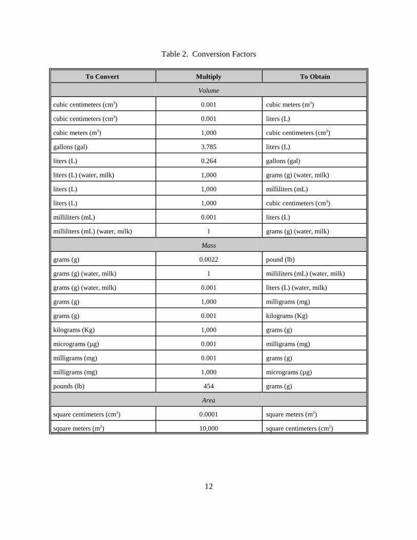
Table 2. Conversion Factors
To Convert Multiply To Obtain
Volume
cubic centimeters (cm3) 0.001 cubic meters (m3)
cubic centimeters (cm3) 0.001 liters (L)
cubic meters (m3) 1,000 cubic centimeters (cm3)
gallons (gal) 3.785 liters (L)
liters (L) 0.264 gallons (gal)
liters (L) (water, milk) 1,000 grams (g) (water, milk)
liters (L) 1,000 milliliters (mL)
liters (L) 1,000 cubic centimeters (cm3)
milliliters (mL) 0.001 liters (L)
milliliters (mL) (water, milk) 1 grams (g) (water, milk)
Mass
grams (g) 0.0022 pound (lb)
grams (g) (water, milk) 1 milliliters (mL) (water, milk)
grams (g) (water, milk) 0.001 liters (L) (water, milk)
grams (g) 1,000 milligrams (mg)
grams (g) 0.001 kilograms (Kg)
kilograms (Kg) 1,000 grams (g)
micrograms (µg) 0.001 milligrams (mg)
milligrams (mg) 0.001 grams (g)
milligrams (mg) 1,000 micrograms (µg)
pounds (lb) 454 grams (g)
Area
square centimeters (cm2) 0.0001 square meters (m2)
square meters (m2) 10,000 square centimeters (cm2)
12

1.4 DEFINITIONS
This section provides definitions for many of the key terms used in these example scenarios. Most of these definitions are taken directly from EPA’s Guidelines for Exposure Assessment (U.S. EPA, 1992a) or EPA’s Exposure Factors Handbook (U.S. EPA, 1997a).
Absorbed Dose - The amount of a substance penetrating across the absorption barriers (the exchange boundaries) of an organism, via either physical or biological processes. This is synonymous with internal dose, which is a more general term denoting the amount absorbed without respect to specific absorption barriers or exchange boundaries. In the calculation of absorbed dose for exposures to contaminated water in bathing, showering or swimming, the outermost layer of the skin is assumed to be an absorption barrier.
Absorption Fraction (ABS, percent absorbed) - The relative amount of a substance that penetrates through a barrier into the body, reported as a percent.
Activity Pattern (time use) Data - Information on activities in which various individuals engage, length of time spent performing various activities, locations in which individuals spend time and length of time spent by individuals within those various environments.
Acute Dose Rate (ADR) - Dose from a single event or average over a limited time period (e.g. 1 day)
Ambient - The conditions surrounding a person, sampling location, etc.
Applied Dose - The amount of a substance presented to an absorption barrier and available for absorption (although not necessarily having yet crossed the outer boundary of the organism).
As Consumed Intake Rates - Intake rates that are based on the weight of the food in the form that it is consumed.
Average Daily Dose (ADD) - Dose rate averaged over a pathway-specific period of exposure expressed as a daily dose on a per-unit-body-weight basis. The ADD is used for exposure to chemicals with non-carcinogenic non-chronic effects. The ADD is usually expressed in terms of mg/kg-day or other mass/mass-time units.
Averaging Time (AT) - The time period over which exposure is averaged.
Bounding Dose Estimate - An estimate of dose that is higher than that incurred by the person in the population with the highest dose. Bounding estimates are useful in developing statements that doses are "not greater than" the estimated value.
13

Central Tendency Dose Estimate - An estimate of dose for individuals within the central portion (average or median) of a dose distribution.
Chronic Intake (exposure) - The long term period over which a substance crosses the outer boundary, is inhaled, or is in contact with the skin of an organism without passing an absorption barrier.
Consumer-Only Intake Rate - The average quantity of food consumed per person in a population composed only of individuals who ate the food item of interest during a specified period.
Contact Rate - General term used to represent rate of contact with a contaminated medium. Contact may occur via ingestion, inhalation, or dermal contact.
Contaminant Concentration (C) - Contaminant concentration is the concentration of the contaminant in the medium (air, food, soil, etc.) contacting the body and has units of mass/volume or mass/mass.
Deposition - The removal of airborne substances to available surfaces that occurs as a result of gravitational settling and diffusion, as well as electrophoresis and thermophoresis; substances at low concentrations in the vapor phase are typically not subject to deposition in the environment.
Distribution - A set of values derived from a specific population or set of measurements that represents the range and array of data for the factor being studied.
Dose - The amount of a substance available for interaction with metabolic processes or biologically significant receptors after crossing the outer boundary of an organism.
Dose Rate - Dose per unit time, for example in mg/day, sometimes also called dosage. Dose rates are often expressed on a per-unit-body-weight basis yielding such units as mg/kg/day. They are also often expressed as averages over some time period (e.g., a lifetime).
Dry Weight Intake Rates - Intake rates that are based on the weight of the food consumed after the moisture content has been removed.
Exposed Foods - Those foods that are grown above ground and are likely to be contaminated by pollutants deposited on surfaces that are eaten.
Exposure - Contact of a chemical, physical, or biological agent with the outer boundary of an organism. Exposure is quantified as the concentration of the agent in the medium in contact integrated over the time duration of the contact.
14

Exposure Assessment - The determination of the magnitude, frequency, duration, and route of exposure.
Exposure Concentration - The concentration of a chemical in its transport or carrier medium at the point of contact.
Exposure Duration (ED) - Total time an individual is exposed to the chemical being evaluated.
Exposure Frequency (EF) - How often a receptor is exposed to the chemical being evaluated.
Exposure Pathway - The physical course a chemical or pollutant takes from the source to the organism exposed.
Exposure Route - The way a chemical or pollutant enters an organism after contact (e.g., by ingestion, inhalation, or dermal absorption).
Exposure Scenario - A set of facts, assumptions, and inferences about how exposure takes place that aids the exposure assessor in evaluating, estimating, or quantifying exposure.
General Population - The total of individuals inhabiting an area or making up a whole group.
Geometric Mean - The nth root of the product of n values.
High-end Dose Estimates - A plausible estimate of individual dose for those persons at the upper end of a dose distribution, conceptually above the 90th percentile, but not higher than the individual in the population who has the highest dose.
Homegrown/Home Produced Foods - Fruits and vegetables produced by home gardeners, meat and dairy products derived form consumer-raised livestock, game meat, and home caught fish.
Inhalation Rate (InhR)- Rate at which air is inhaled. Typically presented in units of m3/hr, m3/day or L/min.
Inhaled Dose - The amount of an inhaled substance that is available for interaction with metabolic processes or biologically significant receptors after crossing the outer boundary of an organism.
Intake - The process by which a substance crosses the outer boundary of an organism without passing an absorption barrier (e.g., through ingestion or inhalation).
Intake Rate (IR) - Rate of inhalation, ingestion, and dermal contact, depending on the route of exposure. For ingestion, the intake rate is simply the amount of food containing the contaminant of interest that an individual ingests during some specific time period (units of mass/time). For
15

inhalation, the intake rate is the inhalation rate (i.e., rate at which air is inhaled). Factors that can affect dermal exposure are the amount of material that comes into contact with the skin, the rate at which the contaminant is absorbed, the concentration of contaminant in the medium, and the total amount of the medium on the skin during the exposure duration.
Internal Dose - The amount of a substance penetrating across absorption barriers (the exchange boundaries) of an organism, via either physical or biological processes (synonymous with absorbed dose).
Lifetime Average Daily Dose (LADD) - Dose rate averaged over a lifetime. The LADD is used for compounds with carcinogenic or chronic effects. The LADD is usually expressed in terms of mg/kg-day or other mass/mass-time units.
Mean Value - The arithmetic average of a set of numbers.
Median Value - The value in a measurement data set such that half the measured values are greater and half are less.
Moisture Content - The portion of foods made up by water. The percent water is needed for converting food intake rates and residue concentrations between whole weight and dry weight values.
Monte Carlo Technique - As used in exposure assessment, repeated random sampling from the distribution of values for each of the parameters in a generic (exposure or dose) equation to derive an estimate of the distribution of (exposures or doses in) the population.
Occupational Tenure - The cumulative number of years a person worked in his or her current occupation, regardless of number of employers, interruptions in employment, or time spent in other occupations.
Per Capita Intake Rate - The average quantity of food consumed per person in a population composed of both individuals who ate the food during a specified time period and those that did not.
Pica - Deliberate ingestion of non-nutritive substances such as soil.
Population Mobility - An indicator of the frequency at which individuals move from one residential location to another.
Potential Dose (PD) - The amount of a chemical which could be ingested, inhaled, or deposited on the skin.
16

Preparation Losses - Net cooking losses, which include dripping and volatile losses, post cooking losses, which involve losses from cutting, bones, excess fat, scraps and juices, and other preparation losses which include losses from paring or coring.
Probabilistic Uncertainty Analysis - Technique that assigns a probability density function to one or more input parameters, then randomly selects values from the distributions and inserts them into the exposure equation. Repeated calculations produce a distribution of predicted values, reflecting the combined impact of variability in each input to the calculation. Monte Carlo is a common type of probabilistic technique.
Recreational/Sport Fishermen - Individuals who catch fish as part of a sporting or recreational activity and not for the purpose of providing a primary source of food for themselves or for their families.
Representativeness - The degree to which a sample is, or samples are, characteristic of the whole medium, exposure, or dose for which the samples are being used to make inferences.
Residential Occupancy Period - The time (years) between a person moving into a residence and the time the person moves out or dies.
Screening-Level Assessments - Typically examine exposures that would fall on or beyond the high end of the expected exposure distribution.
Serving Sizes - The quantities of individual foods consumed per eating occasion. These estimates may be useful for assessing acute exposures.
Subchronic Intake - A period over which intake occurs that is less than or equal to 7 years in duration.
Subsistence Fishermen - Individuals who consume fresh caught fish as a major source of food.
Transfer Fraction (TF) - The fraction of chemical that is transferred to the skin from contaminated surfaces in contact with that surface.
Upper-Percentile Value - The value in a measurement data set that is at the upper end of the distribution of values.
Uptake - The process by which a substance crosses an absorption barrier and is absorbed into the body.
17

2.0
2.1
2.1.1
2.1.2
(Eq. 4)
where:
= /
C = ( /g);
IR = (g/ /day);
EF = ED = AT =
EXAMPLE INGESTION EXPOSURE SCENARIOS
PER CAPITA INGESTION OF CONTAMINATED HOMEGROWN VEGETABLES: GENERAL POPULATION (ADULTS), CENTRAL TENDENCY, LIFETIME AVERAGE EXPOSURE
Introduction
At sites where there is localized soil or water contamination, or where atmospheric fallout of contaminants has been observed or is expected, the potential may exist for uptake of contaminants by locally grown produce. This may result in exposure among local populations via ingestion of vegetables grown in the contaminated area. Receptors could include nearby farming families or home-gardeners and their families, who consume produce grown in the contaminated area. Exposure via intake of contaminated vegetables considers not only the concentrations of contaminants in the food item(s) of concern, but also the rate at which the food is consumed, and the frequency and duration of exposure. For the purposes of this example, exposure via contaminated vegetables is assumed. Lifetime average daily exposure from the ingestion of homegrown vegetables is evaluated for the general population (adults).
Exposure Algorithm
Exposure via this pathway would be calculated as follows:
LADDPOT veg ing potential lifetime average daily dose from ingestion of contaminated vegetables at a contaminated site (mg kg-day);
veg concentration of contaminant in the homegrown vegetables from the site mg
veg per capita intake rate of vegetables homegrown at the site kg
exposure frequency (days/year); exposure duration (years); and averaging time (days).
18
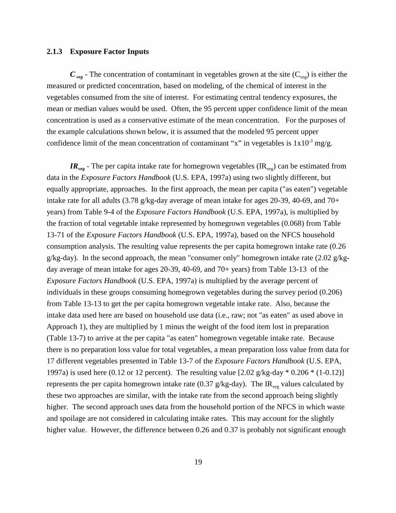
2.1.3 Exposure Factor Inputs
C veg - The concentration of contaminant in vegetables grown at the site (C ) is either the veg
measured or predicted concentration, based on modeling, of the chemical of interest in the vegetables consumed from the site of interest. For estimating central tendency exposures, the mean or median values would be used. Often, the 95 percent upper confidence limit of the mean concentration is used as a conservative estimate of the mean concentration. For the purposes of the example calculations shown below, it is assumed that the modeled 95 percent upper confidence limit of the mean concentration of contaminant “x” in vegetables is 1x10⁻³ mg/g.
IRveg - The per capita intake rate for homegrown vegetables (IRveg) can be estimated from data in the Exposure Factors Handbook (U.S. EPA, 1997a) using two slightly different, but equally appropriate, approaches. In the first approach, the mean per capita ("as eaten") vegetable intake rate for all adults (3.78 g/kg-day average of mean intake for ages 20-39, 40-69, and 70+ years) from Table 9-4 of the Exposure Factors Handbook (U.S. EPA, 1997a), is multiplied by the fraction of total vegetable intake represented by homegrown vegetables (0.068) from Table 13-71 of the Exposure Factors Handbook (U.S. EPA, 1997a), based on the NFCS household consumption analysis. The resulting value represents the per capita homegrown intake rate (0.26 g/kg-day). In the second approach, the mean "consumer only" homegrown intake rate (2.02 g/kg-day average of mean intake for ages 20-39, 40-69, and 70+ years) from Table 13-13 of the Exposure Factors Handbook (U.S. EPA, 1997a) is multiplied by the average percent of individuals in these groups consuming homegrown vegetables during the survey period (0.206) from Table 13-13 to get the per capita homegrown vegetable intake rate. Also, because the intake data used here are based on household use data (i.e., raw; not "as eaten" as used above in Approach 1), they are multiplied by 1 minus the weight of the food item lost in preparation (Table 13-7) to arrive at the per capita "as eaten" homegrown vegetable intake rate. Because there is no preparation loss value for total vegetables, a mean preparation loss value from data for 17 different vegetables presented in Table 13-7 of the Exposure Factors Handbook (U.S. EPA, 1997a) is used here (0.12 or 12 percent). The resulting value [2.02 g/kg-day * 0.206 * (1-0.12)] represents the per capita homegrown intake rate (0.37 g/kg-day). The IRveg values calculated by these two approaches are similar, with the intake rate from the second approach being slightly higher. The second approach uses data from the household portion of the NFCS in which waste and spoilage are not considered in calculating intake rates. This may account for the slightly higher value. However, the difference between 0.26 and 0.37 is probably not significant enough
19

to result in a major impact in estimated exposures. Table 3 shows a comparison of these two approaches.
Table 3. Homegrown Vegetable Intake Rates.
Data Source Input Data Intake Rate
Approach 1 CSFII - Per Capita Total Vegetable Intake “as eaten” (Table 9-4; Average of Means for Ages 2039, 40-69, and 70+ Years) * Fraction Homegrown (Table 13-71).
3.78g/kg-day * 0.068 = 0.26 g/kg-day
Approach 2 NFCS - Consumer Only Homegrown Intake Rate (Table 13-13; Average of Means for Ages 20-39, 40-69, and 70+ years) * Mean Fraction of Individuals in 3 Adult Age Groups Consuming Homegrown Vegetables During Survey (Table 1313) * 1- Preparation Loss Fraction (Table 13-7).
2.02 g/kg-day * 0.206 * (1-0.12) =
0.37 g/kg-day
EF - Exposure frequency (EF) is 365 days a year because the data used in estimating IRveg
are assumed to represent average daily intake over the long-term (i.e., over a year).
ED - Exposure duration (ED) is the length of time over which exposure occurs. For the purposes of this example, the average residency time of the household is assumed. Based on the recommendations in Table 15-174 of the Exposure Factors Handbook (U.S. EPA, 1997a), the 50th percentile residence time is 9 years. Thus, the assumption in this example is that the exposed population consumes homegrown vegetables that have become contaminated on the site at which they reside for 9 years. After that time, they are assumed to reside in a location where the vegetables are not affected by contamination from the site.
AT - Because the lifetime average daily dose is being calculated for a member of the general population, the averaging time (AT) is equivalent to the lifetime of the individual being evaluated. For the purposes of this example, the average lifetime for men and women is used because the exposures are assumed to reflect the general population and are not gender- or age-specific. This value is assumed to be 70 years. For use in the calculations, this value is converted to 25,550 days (i.e., 70 years * 365 days/year).
20

2.1.4 Calculations
Using the exposure algorithm and exposure factor inputs shown above, the LADDPOT veg ing
would be as follows using either Approach 1 or Approach 2 for calculating IRveg for the general population.
Approach 1
Approach 2
2.1.5 Exposure Characterization and Uncertainties
The example presented here is used to represent central tendency exposures among the adult general population from the ingestion of contaminated vegetables. High-end exposures may be estimated by replacing the mean intake rates and residence time used here with upper-percentile intake rates and residence time from the Exposure Factors Handbook (U.S. EPA,
21
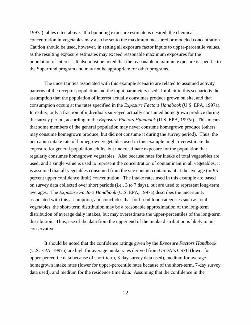
1997a) tables cited above. If a bounding exposure estimate is desired, the chemical concentration in vegetables may also be set to the maximum measured or modeled concentration. Caution should be used, however, in setting all exposure factor inputs to upper-percentile values, as the resulting exposure estimates may exceed reasonable maximum exposures for the population of interest. It also must be noted that the reasonable maximum exposure is specific to the Superfund program and may not be appropriate for other programs.
The uncertainties associated with this example scenario are related to assumed activity patterns of the receptor population and the input parameters used. Implicit in this scenario is the assumption that the population of interest actually consumes produce grown on site, and that consumption occurs at the rates specified in the Exposure Factors Handbook (U.S. EPA, 1997a). In reality, only a fraction of individuals surveyed actually consumed homegrown produce during the survey period, according to the Exposure Factors Handbook (U.S. EPA, 1997a). This means that some members of the general population may never consume homegrown produce (others may consume homegrown produce, but did not consume it during the survey period). Thus, the per capita intake rate of homegrown vegetables used in this example might overestimate the exposure for general population adults, but underestimate exposure for the population that regularly consumes homegrown vegetables. Also because rates for intake of total vegetables are used, and a single value is used to represent the concentration of contaminant in all vegetables, it is assumed that all vegetables consumed from the site contain contaminant at the average (or 95 percent upper confidence limit) concentration. The intake rates used in this example are based on survey data collected over short periods (i.e., 3 to 7 days), but are used to represent long-term averages. The Exposure Factors Handbook (U.S. EPA, 1997a) describes the uncertainty associated with this assumption, and concludes that for broad food categories such as total vegetables, the short-term distribution may be a reasonable approximation of the long-term distribution of average daily intakes, but may overestimate the upper-percentiles of the long-term distribution. Thus, use of the data from the upper end of the intake distribution is likely to be conservative.
It should be noted that the confidence ratings given by the Exposure Factors Handbook (U.S. EPA, 1997a) are high for average intake rates derived from USDA’s CSFII (lower for upper-percentile data because of short-term, 3-day survey data used), medium for average homegrown intake rates (lower for upper-percentile rates because of the short-term, 7-day survey data used), and medium for the residence time data. Assuming that the confidence in the
22
exposure concentration is also at least medium, confidence in the overall central tendency exposure example provided here should also be at least medium.
23
2.2
2.2.1
area. consume home produced tomatoes.
2.2.2
(Eq. 5)
where:
ADD = /
Ctomato =
IRtomato = ( / ); DW =
EF = ED = AT =
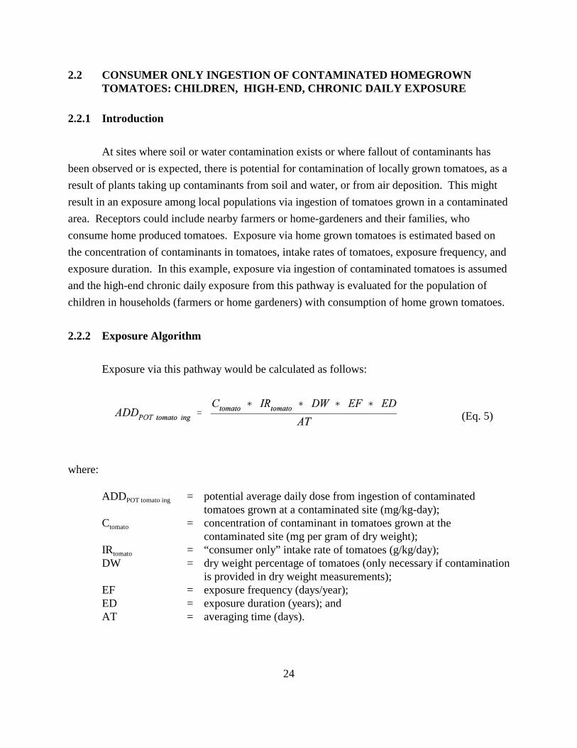
CONSUMER ONLY INGESTION OF CONTAMINATED HOMEGROWN TOMATOES: CHILDREN, HIGH-END, CHRONIC DAILY EXPOSURE
Introduction
At sites where soil or water contamination exists or where fallout of contaminants has been observed or is expected, there is potential for contamination of locally grown tomatoes, as a result of plants taking up contaminants from soil and water, or from air deposition. This might result in an exposure among local populations via ingestion of tomatoes grown in a contaminated
Receptors could include nearby farmers or home-gardeners and their families, who Exposure via home grown tomatoes is estimated based on
the concentration of contaminants in tomatoes, intake rates of tomatoes, exposure frequency, and exposure duration. In this example, exposure via ingestion of contaminated tomatoes is assumed and the high-end chronic daily exposure from this pathway is evaluated for the population of children in households (farmers or home gardeners) with consumption of home grown tomatoes.
Exposure Algorithm
Exposure via this pathway would be calculated as follows:
POT tomato ing potential average daily dose from ingestion of contaminated tomatoes grown at a contaminated site (mg kg-day); concentration of contaminant in tomatoes grown at the contaminated site (mg per gram of dry weight); “consumer only” intake rate of tomatoes g/kg daydry weight percentage of tomatoes (only necessary if contamination
is provided in dry weight measurements); exposure frequency (days/year); exposure duration (years); and averaging time (days).
24
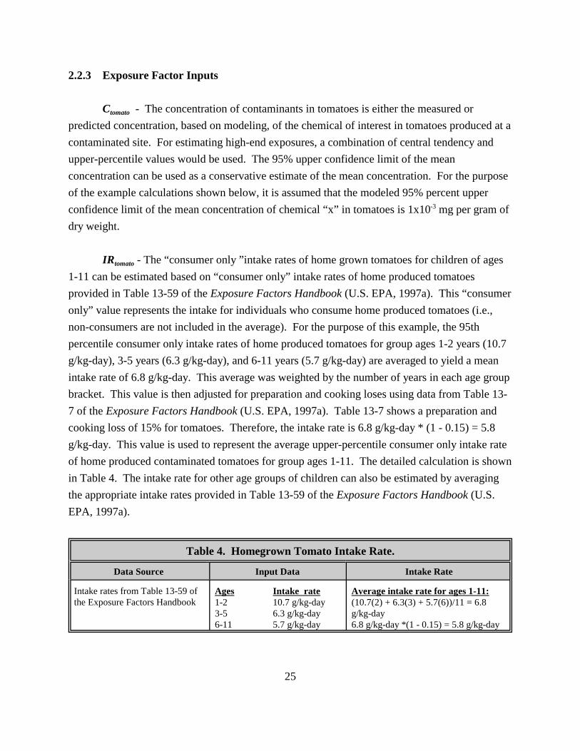
2.2.3 Exposure Factor Inputs
Ctomato - The concentration of contaminants in tomatoes is either the measured or predicted concentration, based on modeling, of the chemical of interest in tomatoes produced at a contaminated site. For estimating high-end exposures, a combination of central tendency and upper-percentile values would be used. The 95% upper confidence limit of the mean concentration can be used as a conservative estimate of the mean concentration. For the purpose of the example calculations shown below, it is assumed that the modeled 95% percent upper confidence limit of the mean concentration of chemical “x” in tomatoes is 1x10⁻³ mg per gram of dry weight.
IRtomato - The “consumer only ”intake rates of home grown tomatoes for children of ages 1-11 can be estimated based on “consumer only” intake rates of home produced tomatoes provided in Table 13-59 of the Exposure Factors Handbook (U.S. EPA, 1997a). This “consumer only” value represents the intake for individuals who consume home produced tomatoes (i.e., non-consumers are not included in the average). For the purpose of this example, the 95th percentile consumer only intake rates of home produced tomatoes for group ages 1-2 years (10.7 g/kg-day), 3-5 years (6.3 g/kg-day), and 6-11 years (5.7 g/kg-day) are averaged to yield a mean intake rate of 6.8 g/kg-day. This average was weighted by the number of years in each age group bracket. This value is then adjusted for preparation and cooking loses using data from Table 137 of the Exposure Factors Handbook (U.S. EPA, 1997a). Table 13-7 shows a preparation and cooking loss of 15% for tomatoes. Therefore, the intake rate is 6.8 g/kg-day * (1 - 0.15) = 5.8 g/kg-day. This value is used to represent the average upper-percentile consumer only intake rate of home produced contaminated tomatoes for group ages 1-11. The detailed calculation is shown in Table 4. The intake rate for other age groups of children can also be estimated by averaging the appropriate intake rates provided in Table 13-59 of the Exposure Factors Handbook (U.S. EPA, 1997a).
Table 4. Homegrown Tomato Intake Rate.
Data Source Input Data Intake Rate
Intake rates from Table 13-59 of the Exposure Factors Handbook
Ages Intake rate 1-2 10.7 g/kg-day 3-5 6.3 g/kg-day 6-11 5.7 g/kg-day
Average intake rate for ages 1-11: (10.7(2) + 6.3(3) + 5.7(6))/11 = 6.8 g/kg-day 6.8 g/kg-day *(1 - 0.15) = 5.8 g/kg-day
25

DW - Dry weight percentage of tomatoes is used to convert units of tomato intake rates from g raw/kg-day to g dry-weight/kg-day. The purpose of this conversion is to ensure consistency between units for concentration data and those for intake rates. The dry weight percentage of raw tomatoes is estimated as one minus the mean moisture content (93.95%) of raw tomatoes provided in Table 9-27 of the Exposure Factors Handbook (U.S. EPA, 1997a). For the purpose of this example, the value of 6.05% as estimated is used to represent the average dry weight percentage of tomatoes.
IREF - Exposure frequency (EF) is 365 days a year because the data used in estimating
tomato are assumed to represent average daily intake over the long term (i.e., over a year).
ED - Exposure duration is the length of time over which exposure occurs. For the purposes of this example, the average residence time of this age group is assumed. Based on the data provided in Table 15-174 of the Exposure Factors Handbook (U.S. EPA, 1997a), the 50th percentile residence time is 9 years. Thus, the assumption in this example is that children in a household with home produced tomato consumption consume tomatoes from a contaminated site for the average residence time of 9 years. After that time, the household is assumed to move to a location where home produced tomatoes are no longer affected by contamination from the site.
AT - Because the average daily dose is being calculated in this example, the averaging time (AT) is equivalent to the exposure duration. As shown above, exposure duration is 9 years; thus the averaging time (AT) is 3,285 days (i.e., 9 years * 365 days/year).
2.2.4 Calculations
Using the exposure algorithm and exposure factors shown above, the ADDPOT tomato ing is estimated as follows for the population of 1-11 year old children who consume home produced tomatoes from a contaminated site.
26

2.2.5 Exposure Characterization and Uncertainties
The example presented here is used to represent high-end exposures among the population of 1-11 year old children from consumption of home grown tomatoes. The population of other age groups of children can also be estimated using appropriate intake rates provided in the Exposure Factors Handbook (U.S. EPA, 1997a) and other parameters provided in the tables cited above. Central tendency exposures may be estimated using mean intake rates from the tables cited above, along with the mean contaminant concentration and residence time. If a bounding exposure estimate is desired, the concentration of contaminant may be set to the maximum measured or modeled concentration. Caution should be used, however, in setting all exposure factor inputs to upper-percentile values, as the resulting exposure estimates may exceed reasonable maximum exposures for the population of interest.
The uncertainties associated with this example scenario are related to the assumed activity pattern of the receptor population and the input parameters used. First, implicit in this scenario is the assumption that the population of children consume tomatoes from a contaminated site at the upper-percentile intake rates of home grown tomatoes specified in the Exposure Factors Handbook (U.S. EPA, 1997a). Second, the intake rates used in this example are based on survey data collected over a short period of time (i.e., 1-3 days) but are used to represent long-term averages. The intake rates collected in such a way might be an appropriate estimate for the short-term and long-term averages. But the distribution of the average intake rates generated using a short-term data might not reflect the long term distribution of the average daily intakes. Thus, there is some degree of uncertainty in using the upper-percentiles of the long-term distribution of intake rates to estimate high-end exposures. Third, a single value for average contaminant concentration in tomatoes is used to estimate high-end chronic exposure. This assumes that all the tomatoes consumed from the site contains contaminant at the average concentration. The variability in average contaminant concentration in tomatoes might introduce some degree of uncertainty here.
The confidence in the high-end exposure provided in this example is related to confidences in upper-percentile intake rates of home produced tomatoes and contaminant concentration. The confidence rating given by the Exposure Factors Handbook (U.S. EPA, 1997a) is low for the distribution of intake rates of home produced tomatoes because the upper-percentiles of the short-term distribution may overestimate intake, and the confidence rating is medium for average residence time. If the rating for the contaminant concentration is medium,
27

the overall confidence rating for the high-end exposure would be expected to be low because of the low confidence in the intake rates.
28

2.3 PER CAPITA INGESTION OF CONTAMINATED BEEF: ADULTS, CENTRAL TENDENCY, LIFETIME AVERAGE EXPOSURE
2.3.1 Introduction
There is potential for contamination (e.g., lipophilic compounds) of meat products such as beef as a result of cattle consuming contaminated forage, silage, grain, soil, or drinking water. This may result in exposure among the general population via consumption of beef that is widely distributed in the market place. Exposure via consumption of contaminated beef is estimated based on the concentration of contaminants in beef, the consumption rate of beef, exposure frequency, and exposure duration. In this example, exposure via contaminated beef is assumed and central tendency lifetime average daily exposure from this pathway is evaluated for the adult general population.
2.3.2 Exposure Algorithm
Exposure via this pathway would be calculated as follows:
where:
LADDPOT beef ing
Cbeef FC IRbeef EF ED AT
= potential lifetime average daily dose from ingestion of contaminated beef (mg/kg-day);
= concentration of contaminant in beef (mg per gram of fat= fat content or fraction of lipid in beef (percent); = per capita intake rate of beef (g/kg/day); = exposure frequency (days/year); = exposure duration (years); and = averaging time (days).
(Eq. 6)
);
29
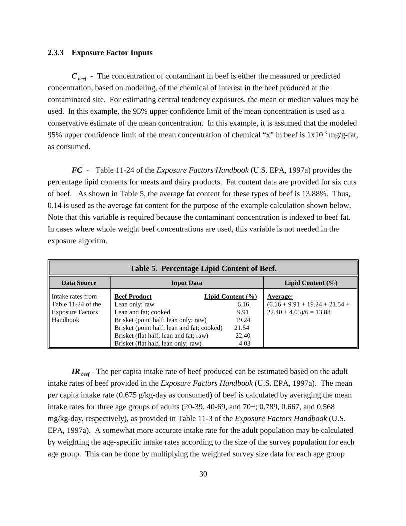
2.3.3 Exposure Factor Inputs
C beef - The concentration of contaminant in beef is either the measured or predicted concentration, based on modeling, of the chemical of interest in the beef produced at the contaminated site. For estimating central tendency exposures, the mean or median values may be used. In this example, the 95% upper confidence limit of the mean concentration is used as a conservative estimate of the mean concentration. In this example, it is assumed that the modeled 95% upper confidence limit of the mean concentration of chemical “x” in beef is 1x10⁻³ mg/g-fat, as consumed.
FC - Table 11-24 of the Exposure Factors Handbook (U.S. EPA, 1997a) provides the percentage lipid contents for meats and dairy products. Fat content data are provided for six cuts of beef. As shown in Table 5, the average fat content for these types of beef is 13.88%. Thus, 0.14 is used as the average fat content for the purpose of the example calculation shown below. Note that this variable is required because the contaminant concentration is indexed to beef fat. In cases where whole weight beef concentrations are used, this variable is not needed in the exposure algoritm.
Table 5. Percentage Lipid Content of Beef.
Data Source Input Data Lipid Content (%)
Intake rates from Table 11-24 of the Exposure Factors Handbook
Beef Product Lipid Content (%) Lean only; raw 6.16 Lean and fat; cooked 9.91 Brisket (point half; lean only; raw) 19.24
Average: (6.16 + 9.91 + 19.24 + 21.54 + 22.40 + 4.03)/6 = 13.88
Brisket (point half; lean and fat; cooked) 21.54 Brisket (flat half; lean and fat; raw) 22.40 Brisket (flat half, lean only; raw) 4.03
IR beef - The per capita intake rate of beef produced can be estimated based on the adult intake rates of beef provided in the Exposure Factors Handbook (U.S. EPA, 1997a). The mean per capita intake rate (0.675 g/kg-day as consumed) of beef is calculated by averaging the mean intake rates for three age groups of adults (20-39, 40-69, and 70+; 0.789, 0.667, and 0.568 mg/kg-day, respectively), as provided in Table 11-3 of the Exposure Factors Handbook (U.S. EPA, 1997a). A somewhat more accurate intake rate for the adult population may be calculated by weighting the age-specific intake rates according to the size of the survey population for each age group. This can be done by multiplying the weighted survey size data for each age group
30
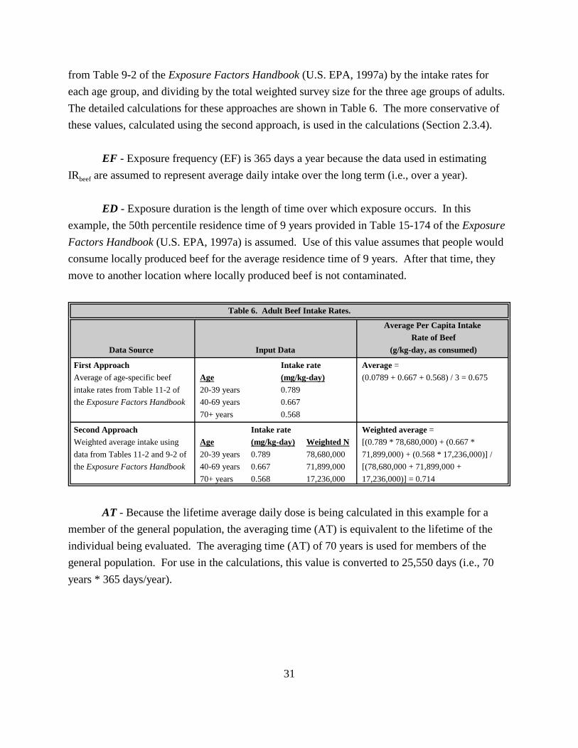
from Table 9-2 of the Exposure Factors Handbook (U.S. EPA, 1997a) by the intake rates for each age group, and dividing by the total weighted survey size for the three age groups of adults. The detailed calculations for these approaches are shown in Table 6. The more conservative of these values, calculated using the second approach, is used in the calculations (Section 2.3.4).
IREF - Exposure frequency (EF) is 365 days a year because the data used in estimating
beef are assumed to represent average daily intake over the long term (i.e., over a year).
ED - Exposure duration is the length of time over which exposure occurs. In this example, the 50th percentile residence time of 9 years provided in Table 15-174 of the Exposure Factors Handbook (U.S. EPA, 1997a) is assumed. Use of this value assumes that people would consume locally produced beef for the average residence time of 9 years. After that time, they move to another location where locally produced beef is not contaminated.
Table 6. Adult Beef Intake Rates.
Average Per Capita Intake Rate of Beef
Data Source Input Data (g/kg-day, as consumed)
First Approach Intake rate Average = Average of age-specific beef Age (mg/kg-day) (0.0789 + 0.667 + 0.568) / 3 = 0.675 intake rates from Table 11-2 of 20-39 years 0.789 the Exposure Factors Handbook 40-69 years 0.667
70+ years 0.568
Second Approach Intake rate Weighted average = Weighted average intake using Age (mg/kg-day) Weighted N [(0.789 * 78,680,000) + (0.667 * data from Tables 11-2 and 9-2 of 20-39 years 0.789 78,680,000 71,899,000) + (0.568 * 17,236,000)] / the Exposure Factors Handbook 40-69 years 0.667 71,899,000 [(78,680,000 + 71,899,000 +
70+ years 0.568 17,236,000 17,236,000)] = 0.714
AT - Because the lifetime average daily dose is being calculated in this example for a member of the general population, the averaging time (AT) is equivalent to the lifetime of the individual being evaluated. The averaging time (AT) of 70 years is used for members of the general population. For use in the calculations, this value is converted to 25,550 days (i.e., 70 years * 365 days/year).
31

2.3.4 Calculations
Using the exposure algorithm and exposure factor inputs shown for the second approach above, the LADDPOT beef ing may be estimated as follows:
2.3.5 Exposure Characterization and Uncertainties
The example presented here is used to represent per capita central tendency exposures among adults from ingestion of contaminated beef. High-end exposures may be estimated by replacing the mean intake rates and residence time used here with upper-percentile values from the tables cited above. In addition, if a bounding exposure estimate is desired, the chemical concentration in beef may also be set to the maximum measured or modeled concentration. However, caution should be used in setting all exposure factor inputs to upper-percentile values, as the resulting exposure estimate might well exceed reasonable maximum exposures for the population of interest.
The uncertainties associated with this example scenario are related to the assumed activity patterns of the receptor population and the input parameters used. First, implicit in this scenario is the assumption that the general population consumes beef at the average rates specified in the Exposure Factors Handbook (U.S. EPA, 1997a). Second, the intake rates used in this example are based on survey data collected over a short period of time (i.e.,1-3 days), but are used to represent long-term averages. The intake rates collected in such a way might be an appropriate estimate for the short-term and long-term averages. The distribution of the average intake rates generated using short-term data might not reflect the long-term distribution of daily intakes. Thus, there is some degree of uncertainty in using the upper percentiles of the long-term distribution of intake rates to estimate high-end exposures.
32

The confidence in the overall central tendency exposure provided in this example is related to confidences in per capita intake rates of beef, residence time, and the exposure concentration. The confidence rating given by the Exposure Factors Handbook (U.S. EPA, 1997a) is high for average intake rates of beef and medium for the residence time of the general population. If the rating for the exposure concentration is also medium, the overall confidence in the central tendency exposure estimated in this example should be at least medium.
33
2.4
2.4.1
2.4.2
(Eq. 7)
where:
ADR milk ing = (mg/
Cmilk = /g); IRmilk = /EF = ED =
= ); and AT =
2.4.3
C -
CONSUMER ONLY INGESTION OF CONTAMINATED DAIRY PRODUCTS: GENERAL POPULATION (ALL AGES COMBINED), BOUNDING, ACUTE EXPOSURE
Introduction
At locations where dairy products are contaminated with toxic chemicals, there is the potential for acute exposure via ingestion of dairy products such as milk, cheese, and cream. Acute exposure via this pathway is estimated based on the concentration of contaminants in dairy products, the intake rate of dairy products per eating occasion, exposure frequency, and exposure duration. In this example, acute exposure via ingestion of milk is assumed and evaluated for the general population.
Exposure Algorithm
Exposure via this pathway would be calculated as follows:
POT acute potential dose rate from ingestion of contaminated milk kg-day);
concentration of contaminants in milk (mgintake rate of milk per eating occasions (g eating occasion); exposure frequency (eating occasions/day); exposure duration (day);
BW body weight (kgaveraging time (day).
Exposure Factor Inputs
milk The concentration of contaminants in milk is either the measured or predicted concentration, based on modeling, of the chemical of interest in milk. For acute exposure, the maximum concentration of chemicals in milk would be used. In this example, it is assumed that
34

the maximum concentration of chemical “x” in milk is 1x10⁻³ mg per gram of milk. Because this is a whole weight concentration (i.e., not a lipid-based value), no lipid fraction value is required in this exposure algorithm.
IRmilk - The intake rate of milk per eating occasion for the general population is provided in Table 11-23 of the Exposure Factors Handbook (U.S. EPA, 1997a). In this example, the 99th percentile of the quantity (as consumed) of milk consumed per eating occasion, 552 g/eating occasion for the general population (i.e., all ages combined), is used for the example calculation shown below to provide a bounding estimate of exposure.
EF - Exposure frequency is assumed to be one eating occasion per day.
ED - Exposure duration is the length of time over which exposure occurs. For assessing acute exposure, the shortest time period which might lead to an acute effect should be used as exposure duration. For the purpose of the example calculation shown below, the exposure duration of one day is used.
BW - Since this scenario is calculating a bounding estimate, a low end body weight would be appropriate. However, only mean values are currently available in the Exposure Factors Handbook (U.S. EPA, 1997a). Therefore, the weighted average body weight of 63.5 kilograms for the general population (all ages combined) may be calculated using data in Tables 7-2 and 7-3 of the Exposure Factors Handbook (U.S. EPA, 1997a), as shown in Table 7. The mean body weight of adults (71.8 kg) is used for ages 18 through 75 (a total of 58 years). The weighted average body weight is then used for the example calculation shown below. This value is used for the example calculation shown below.
35

Table 7. Weighted Average Body Weight (Ages 1-75).
Data Source Input Data Weighted average:
Body weight data from Tables 7-2 and 7-3 of the Exposure Factors Handbook
Age-specific body weight 1 year 11.3 kg 2 years 13.3 kg 3 years 15.3 kg 4 years 17.4 kg 5 years 19.7 kg 6 years 22.6 kg 7 years 24.9 kg 8 years 28.1 kg 9 years 31.5 kg 10 years 36.3 kg 11 years 41.1 kg 12 years 45.3 kg 13 years 50.4 kg 14 years 56.0 kg 15 years 58.1 kg 16 years 62.6 kg 17 years 63.2 kg 18-75 years 71.8 kg
[11.3 + 13.3 + 15.3 + 17.4 + 19.7 + 22.6 + 24.9 + 28.1 + 31.5 + 36.3 + 41.1 + 45.3 + 50.4 + 56.0 + 58.1 + 62.6 + 63.2 + (71.8 * 58)] / 75 = 63.5 kg
AT - For acute exposure assessment, averaging time is equal to exposure duration. Thus, the averaging time of one day is used in this example.
2.4.4 Calculations
Using the exposure algorithm and exposure factors shown above, ADRPOT milk ing is estimated as follows for the general population:
36

2.4.5 Exposure Characterization and Uncertainties
The example presented here is used to represent acute exposure among the general population (i.e., all ages combined) from ingestion of contaminated milk at one eating occasion. Acute exposures via ingestion of other dairy products such as cream, cheese, and eggs for different age groups or populations may also be estimated by using the corresponding input parameters in the tables cited above.
It should be noted that in this scenario, considerable category lumping was performed to assess the general population and to make use of particular data sets from the Exposure Factors Handbook. In many exposure cases, however, it may not be useful to lump or aggregate groups where there are susceptibility differences by age, sex or other category. While lumping may be useful for conducting a first scoping assessment, caution should be used when lumping groups into aggregate categories that have no biological meaning.
The confidence in the acute exposure estimate provided in this example is related to confidences in the 99th percentile intake rate of milk per eating occasion and the exposure concentration. The confidence rating for the intake rate of milk is expected to be medium, as the intake rates of milk per eating occasion are estimated based on the 1977-78 USDA NFCS (National Food Consumption Survey) data. According to the Exposure Factors Handbook (U.S. EPA, 1997a), the USDA NFCS data were collected from interviews of 37,874 individuals, but are relatively old and do not consider recent changes in dietary habits. Thus, if the confidence rating for the exposure concentration is medium or higher, the overall confidence rating for acute exposure should be at least medium.
37

2.5 INGESTION OF CONTAMINATED DRINKING WATER: OCCUPATIONAL ADULTS, BASED ON OCCUPATIONAL TENURE, HIGH-END, LIFETIME AVERAGE EXPOSURE
2.5.1 Introduction
At sites where surface water or ground water, that is used as a source of potable water, is contaminated, there may be the potential for exposure via ingestion of drinking water. Receptors could include any population who consumes tap water from a contaminated site. Exposure via ingestion of contaminated drinking water is estimated based on the concentration of contaminants in drinking water, the intake rate of drinking water, exposure frequency, and exposure duration. In this example, exposure via ingestion of drinking water is assumed and the high-end chronic lifetime daily exposure from this pathway is evaluated for an adult occupational population of farm workers.
2.5.2 Exposure Algorithm
Exposure via this pathway would be calculated as follows:
(Eq. 8)
where:
LADDPOT drinking water ing = potential lifetime average daily dose from ingestion of
IRC
contaminated drinking water (mg/kg-day); drinking water = concentration of contaminant in drinking water (mg/mL);
drinking water = intake rate of drinking water (mL/kg-day);EF = exposure frequency (days/year);ED = exposure duration (years); andAT = averaging time (days).
2.5.3 Exposure Factor Inputs
Cdrinking water - The concentration of contaminants in drinking water is either the measured or predicted concentration, based on modeling, of the chemical of interest in the tap water
38

supplied from a contaminated site. For estimating central tendency exposures, the mean or median values would be used. The 95% upper confidence limit of the mean concentration can be used as a conservative estimate of the mean concentration. For the purpose of the example calculations shown below, it is assumed that the modeled 95% upper confidence limit of the mean concentration of chemical “x” in drinking water is 1x10⁻³ mg/mL.
IRdrinking water - Table 3-30 of the Exposure Factors Handbook (U.S. EPA, 1997a) provides recommended drinking water intake rates. For the purpose of the example calculation, the upper-percentile (i.e., 90th percentile) drinking water intake rate of 34 mL/kg-day recommended for adults in Table 3-30 is selected to represent the average intake rate of contaminated drinking water for the occupational population of farm workers. It is assumed in this example that farm workers always consume the tap water supplied to their farms, as a sole source of drinking water during working hours.
estimating IREF - Exposure frequency is 365 days a year for this example because the data used in
drinking water are assumed to represent average daily intake over the long term (i.e., over a year).
ED - Exposure duration is the length of time over which exposure occurs. For the purposes of this example, the occupational tenure of 39.8 years for the 65+ (years) age group for farming provided in Table 15-161 of the Exposure Factors Handbook (U.S. EPA, 1997a) is assumed. This age group is selected because it represents the total occupational tenure by the end of a working lifetime. This value assumes that farm workers consume the tap water from a contaminated source during working hours for the average farming occupational tenure of 39.8 years. After that, they either retire or move to a location where the tap water they consume is no longer contaminated.
AT - Because the lifetime average daily dose is being calculated in this example for a members of the general population, the averaging time (AT) is equivalent to the lifetime of the individuals being evaluated. The averaging time (AT) of 70 years is used for a member of the general population. For use in the calculations, this value is converted to 25,550 days (i.e., 70 years * 365 days/year).
39

2.5.4 Calculations
Using the exposure algorithm and exposure factors shown above, the LADDPOT drinking water
ing is estimated as follows for the population of farm workers:
2.5.5 Exposure Characterization and Uncertainties
The example presented here is used to represent high-end exposure among the population of farm workers via ingestion of drinking water. Central tendency exposures may be estimated using mean or median intake rates from the table cited above. If a bounding exposure estimate is desired, the concentration of contaminant may be set to the maximum measured or modeled concentration. Caution should be used, however, in setting all exposure factor inputs to upper-percentile values, as the resulting exposure estimates may exceed reasonable maximum exposures for the population of interest.
The uncertainties associated with this example scenario are related to the assumed activity pattern of the receptor and the input parameters used. First, implicit in this scenario is the assumption that farm workers only consume tap water to satisfy their physiological need for water. In reality, farm workers might consume bottled water or canned beverage (which is not contaminated) to relieve thirst during working hours. Thus, use of the intake rates provided in the Exposure Factors Handbook (U.S. EPA, 1997a) might overestimate exposure of the farm workers via ingestion of drinking water. In addition, some wells may have some sort of treatment that may remove contaminants. On the other hand, farm workers that work in high-temperature environments or engage in activities that are physically demanding, may have higher levels of tapwater intake. For these individuals, exposure may be underestimated. Second, the upper-percentile intake rates of drinking water used in this example are derived from the data collected from a short period of time (3 days). The extrapolation to chronic intake in this
40

example might introduce some degree of uncertainty. There may also be seasonal or regional differences in drinking water intake that add to the uncertainty in these estimates. Third, a single value for contaminant concentration (i.e., 95% upper confidence limit of the mean) in drinking water is used to estimate high-end chronic exposure. This assumes that drinking water always contains a contaminant at the average concentration. The variability in contaminant concentrations obtained from different samples introduces some degree of uncertainty.
The confidence in the high-end exposure estimate provided in this example is related to confidences in average intake rates of drinking water, the occupational tenure, and exposure concentrations. The confidence rating given by the Exposure Factors Handbook (U.S. EPA, 1997a) is medium for the intake rates of drinking water and high for the occupational tenure. Thus, if the confidence rating for the exposure concentration is medium, the overall confidence rating for the high-end exposure is at least medium.
41

2.6
2.6.1
Receptors
school.
2.6.2
(Eq. 9)
where:
ADD = /
C = /IR = /ET = ); EF = ED = AT =
INGESTION OF CONTAMINATED DRINKING WATER: SCHOOL CHILDREN, CENTRAL TENDENCY, SUBCHRONIC EXPOSURE
Introduction
At sites where surface water or ground water, that is used as a source of potable water, is contaminated, there is the potential for exposure via ingestion of drinking water. could include any population who consumes tap water from a contaminated site. Exposure via ingestion of contaminated drinking water is estimated based on the concentration of contaminants in drinking water, the intake rate of drinking water, exposure frequency, and exposure duration. In this example, exposure via ingestion of drinking water is assumed and the central tendency subchronic average daily exposure from this pathway is evaluated for the population of elementary school children, ages 5-10. It is assumed that the school children’s home drinking water supplies are not contaminated and thus, the children are exposed only at
Exposure Algorithm
Exposure via this pathway would be calculated as follows:
POT drinking water ing potential average daily dose from ingestion of contaminated drinking water (mg kg-day);
drinking water concentration of contaminant in drinking water (mg mL); drinking water intake rate of drinking water (mL kg-hour);
exposure time (hours/dayexposure frequency (days/year); exposure duration (years); and averaging time (days).
42

2.6.3 Exposure Factor Inputs
Cdrinking water - The concentration of contaminants in drinking water is either the measured or predicted concentration, based on modeling, of the chemical of interest in the tap water supplied from a contaminated site. For estimating central tendency exposures, the mean or median values would be used. The 95% upper confidence limit of the mean concentration can be used as a conservative estimate of the mean concentration. For the purpose of the example calculations shown below, it is assumed that the modeled 95% upper confidence limit of the mean concentration of chemical “x” in drinking water is 1x10⁻³ mg/mL.
IR drinking water - The tap water intake rate for elementary school children (5-10 years old) is estimated first by averaging the mean tap water intake rates for children of ages 4-6 and ages 710 years provided in Table 3-7 of the Exposure Factors Handbook (U.S. EPA, 1997a). The weighted average is calculated by multiplying each consumption in each age category by the number of years in the age bracket and dividing by the total number of years. The weighted average is then divided by 14 hours/day to yield the hourly intake rate of drinking water for children of ages 4-10 years. This assumes that children in this age group sleep 10 hours per day (see Table 15-83 of the Exposure Factors Handbook (U.S. EPA, 1997a)). Thus, drinking water is only consumed over the 14 hours that children are awake. The value of 2.3 mL/kg-hour, as estimated, is used to represent the intake rate of drinking water for elementary school children (510 years old). The detailed calculation is shown in Table 8 below. It should be noted that these values are based on data that include the use of tap water in preparing foods and other beverages (i.e., juices prepared with water).
Table 8. Drinking Water Intake Rate for School Children (Ages 4-10).
Data Source Input Data Intake Rate
Table 3-7 of the Exposure Factors Handbook
Age (yrs) Total tap water intake rate 4 - 6 37.9 mL/kg-day 7- 10 26.9 mL/kg-day
Intake rate for ages 4-10 yrs: (37.9(3) + 26.9(4))/7 = 31.6 mL/kg-day 31.6/14hrs/day = 2.3 mL/kg-hour
ET- According to Table 15-84 of the Exposure Factors Handbook (U.S. EPA, 1997a), the median and mean number of minutes spent in school for 5-11 year old children is approximately 390 minutes (i.e., 6.5 hours). Since data are not specifically available for 5-10
43

year olds, the value of 6.5 hours for the 5-11 years old range is used for the example calculation shown below.
EF - Exposure frequency is assumed to be 185 days a year for this example. This is equivalent to 37 weeks of full-time school, and accounts for 15 weeks off for summer and winter vacations, Federal and school holidays, etc.
ED - Exposure duration is the length of time over which exposure occurs. For the purposes of this example, the exposure duration for 5-10 year old school children is assumed to be six years (i.e., from kindergarten through fifth grade). This assumes that all six years are spent in the same school where tap water contamination exists.
AT - For assessment of average daily dose, the averaging time is equal to the exposure duration. Thus, for the purpose of the example calculation shown below, the averaging time of 6 years, or 2,190 days, is used.
2.6.4 Calculations
Using the exposure algorithm and exposure factors shown above, the LADDPOT drinking water
ing is estimated as follows for the population of elementary school children:
2.6.5 Exposure Characterization and Uncertainties
The example presented here is used to represent central tendency exposure among the population of elementary school children, ages 5-10, via ingestion of contaminated drinking water. High-end exposures may be estimated by using upper-percentile values of intake rates and exposure time from the tables cited above. If a bounding exposure estimate is desired, the concentration of contaminant may also be set to the maximum measured or modeled
44

concentration. Caution should be used, however, in setting all exposure factor inputs to upper-percentile values, as the resulting exposure estimates may exceed reasonable maximum exposures for the population of interest.
The uncertainties associated with this example scenario are related to the assumed activity pattern of the receptor and the input parameters used. First, implicit in this scenario is the assumption that school children consume only tap water to satisfy their physiological need for water. In reality, children might bring bottled water or juice which has been reconstituted with water from another source (which is not contaminated) to school. This might overestimate exposure via ingestion of drinking water. Second, elementary school children often change schools as their parents change jobs or buy new houses. The use of six years for exposure duration might overestimate the exposure for some children. Third, intake rates of drinking water found in the Exposure Factors Handbook (U.S. EPA, 1997a) are derived from the data collected from a short period of time (3 days). The extrapolation to chronic intake in this example might introduce some degree of uncertainty. Fourth, many schools have before or after school activities such as on-site extended care (which is particularly important for working families) or athletic/sports programs during which water consumption would be increased. The omission of these programs might underestimate exposure via ingestion of drinking water. Fifth, children attending summer school would have a greater exposure frequency. The omission of this uncertainty could also underestimate exposure via ingestion of drinking water.
The confidence in the central tendency exposure estimate provided in this example is related to confidences in average intake rates of drinking water, the activity pattern data used to estimate the exposure time, and the exposure concentration. The confidence rating given by the Exposure Factors Handbook (U.S. EPA, 1997a) is medium for the tap water intake rate and high for the activity pattern data. Thus, if the confidence in the exposure concentration is medium, the overall confidence rating for the central tendency exposure would be at least medium.
45

2.7
2.7.1
Receptors
2.7.2
(Eq. 10)
where:
= /
C = /
CF = ; IR =
INGESTION OF CONTAMINATED DRINKING WATER: ADULT MALES IN HIGH PHYSICAL ACTIVITY OCCUPATIONS, BOUNDING, AVERAGE LIFETIME EXPOSURE
Introduction
At sites where ground water or surface water, that is used as a source of potable water, is contaminated, there is the potential for exposure via ingestion of drinking water. could include any population who consumes tap water from a contaminated site. Increased rates of drinking water ingestion may occur among populations engaging in highly physically demanding activities or those who work in high temperature conditions. Exposure via ingestion of contaminated drinking water is estimated based on the concentration of contaminants in drinking water, intake rates of drinking water, exposure frequency, and exposure duration. In this example, exposure via ingestion of contaminated drinking water is assumed, and the bounding lifetime average daily exposure from this pathway is evaluated for the population of steel mill workers who consume more water than the general population because of their high level of physical activity and the high temperature working environment.
Exposure Algorithm
Exposure via this pathway would be calculated as follows:
LADDPOT drinking water ing potential lifetime average daily dose from ingestion of contaminated drinking water (mg kg-day);
drinking water concentration of contaminants in contaminated drinking water (mg mL); conversion factor for 1,000 mL/L
drinking water intake rate of drinking water (L/day);
46
EF = exposure frequency (days/year); ED = exposure duration (years); BW = average body weight for the population of interest (kg); and AT = averaging time (days).
2.7.3 Exposure Factor Inputs
Cdrinking water - The concentration of contaminants in drinking water is either the measured or predicted concentration, based on modeling, of the chemical of interest in the drinking water supplied from a contaminated site. For a bounding exposure estimate, the maximum concentration of contaminant in drinking water would be used. For the purpose of the example calculations shown below, it is assumed that the maximum concentration of chemical “x” in drinking water is 1x10⁻³ mg/mL.
CF - A conversion factor of 1,000 is needed to convert liters to milliliters for the purposes of calculating a LADD.
IRdrinking water - According to Table 3-27 and the corresponding text of the Exposure Factors Handbook (U.S. EPA, 1997a), the mean water intake rate for a male adult working at a high level of physical activity and at an ambient temperature of 95 oF is 0.54 L/hour. It is assumed that all steel mill workers are male and those being evaluated work for eight hours a day under a high level of physical activity and at a high temperature. Thus, the average daily intake rate of drinking water during working hours is estimated to be 4.32 L/day by multiplying the hourly intake rate of 0.54 L/hours by 8 hours/day. This value is used for the example calculation shown below.
EF – Exposure frequency is assumed to be 219 days a year for this example. This estimate assumes that steel mill workers work 5 days a week, observe 10 Federal holidays, take 4 weeks of vacation a year and an additional 12 personal days per year. This value is one of those recommended by U.S. EPA (1989) to represent central tendency exposure frequency for industrial workers.
ED - Exposure duration is the length of time over which exposure occurs. For the purposes of this example, the occupational tenure of 18.1 years for the 55-64 (years) age group of Operators, Fabricators, and Laborers provided in Table 15-161 of the Exposure Factors
47

Handbook (U.S. EPA, 1997a) is assumed. This value assumes that steel mill workers consume contaminated tap water during working hours for the average occupational tenure of 18.1 years. After that, they either retire or change their occupation and no longer consume the contaminated tap water in the steel mill.
BW - The average male adult body weight of 78.1 kilogram is provided in Table 7-4 of the Exposure Factors Handbook (U.S. EPA, 1997a). This value is used for the example calculations shown below.
AT - Because the lifetime average daily dose is being calculated in this example for a member of the general population, the averaging time (AT) is equivalent to the lifetime of the individual being evaluated. The averaging time (AT) of 70 years is used for members of the general population. For use in the calculations shown below, this value is converted to 25,550 days (i.e., 70 years * 365 days/year).
2.7.4 Calculations
Using the exposure algorithm and exposure factors shown above, the LADDPOT drinking water
ing is estimated as follows for the population of steel mill workers:
2.7.5 Exposure Characterization and Uncertainties
The example presented here is used to represent bounding exposure via ingestion of drinking water among the population of steel mill workers that engage in a high level of physical activity in high temperature environments. Central tendency exposures may be estimated using the lower drinking water intake rates from the table cited above and an average concentration of contaminant in drinking water. It should be noted that caution should be used in setting all
48
exposure factor inputs to upper-percentile values, as in this example, because the resulting exposure estimates may exceed reasonable maximum exposures for the population of interest.
The uncertainties associated with this example scenario are related to the assumed activity pattern of the receptor population and the input parameters used. First, implicit in this scenario is the assumption that steel mill workers only consume tap water to satisfy their physiological need for water. In reality, the workers might consume bottled water or canned juice which is not contaminated. Thus, exposure estimates presented in this example might have overestimated real exposures of the steel mill workers via ingestion of drinking water. Second, in this example, the average occupational tenure of 18.1 years for 55-64 is used to represent exposure duration. The use of the occupational tenure here assumes that steel mill workers work in the same steel mill during their entire occupational tenure. In reality, steel mill workers might transfer to another steel mill where tap water is not contaminated. Thus, the bounding exposure estimate based on the occupational tenure might overestimate the exposure for the general population of steel mill workers. Third, the intake rates of drinking water used in this example are based on the study on physiological demands of male adults for water at different temperatures and under different levels of physical activity. This study was conducted on only 7 -18 adult males. Thus, the intake rates are not fully representative of the general population of workers in high temperature, high physically-demanding jobs. Fourth, the discussion of tap water consumption does not address the potential that some of the steel mill workers may live near the site and continue to draw their water supply from a contaminated groundwater source. If this did occur, it would result in underestimating an individual’s exposure.
The confidence in the bounding exposure estimate provided in this example is related to confidences in average intake rates of drinking water, occupational tenure, and exposure concentrations. The confidence rating given by the Exposure Factors Handbook (U.S. EPA, 1997a) is high for the occupational tenure, but is not given for the intake rates of drinking water for high physical activities, as the study is listed as a relevant study rather than a key study. Since the intake rate of drinking water is derived from a small sample (7-18 male adults), the confidence rating is presumably low. Thus, even if the rating for the exposure concentration is high, the overall confidence rating for the bounding exposure is expected to be low.
49

2.8 INCIDENTAL INGESTION OF POOL WATER: CHILDREN, BOUNDING, ACUTE EXPOSURE
2.8.1 Introduction
In some situations it is necessary to assess exposure/risk to individuals from biocides or other chemicals in swimming pools. Both adults and children may incidentally ingest chemicals in the water when swimming or wading. These chemicals may either be soluble or insoluble. Depending on the density of the chemical, it could either be floating on the surface of water or it could sink to the bottom. Receptors could include swimmers or waders in home swimming pools.
Acute exposure via incidental intake of contaminated surface water considers not only the concentration of contaminant in the water, but also the ingestion rate, and the duration of exposure. A bounding exposure for acute incidental ingestion of pool water is evaluated for children (ages 5-11 years).
2.8.2 Exposure Algorithm
Exposure via this pathway would be calculated as follows:
(Eq. 11)
where:
ADRPOT pool water ing = acute potential dose rate from incidental ingestion of contaminated pool water (mg/kg-day);
Cpool water IRpool water ET
= = =
concentration of contaminant in the pool water (mg/L); intake rate (L/hr); exposure time (hours/event);
EF = exposure frequency (events/day); ED = exposure duration (day); AT = averaging time (days); and, BW = body weight (kg).
50
2.8.3 Exposure Factor Inputs
Cpool water - The concentration of contaminant in pool water at the site (Cpool water) is either the measured or predicted concentration, based on modeling, of the chemical of interest in the pool water consumed. For estimating acute exposures, the maximum value would be used. For the purposes of the example calculations shown below, it is assumed that the modeled maximum concentration of chemical “x” in pool water is 1x10⁻³ mg/L.
IRpool water - Intake rate (IR) for the swimmer is assumed to be 50 mL/hour or 0.05 L/hr (U.S. EPA, 1989) for the purposes of this example. Note that this is based on a noncompetitive swimming scenario. Competitive swimming may increase this rate by 3-4 times. It would be more likely that competitive swimming events would not be held in home swimming pools. Note that the EPA’s proposed Water Quality Guidance for the Great Lakes (58FR20869) has proposed 30 ml/hour as an incidental ingestion rate for swimmers.
ET - The exposure time (ET) can be estimated using statistics from Table 15-67 of the Exposure Factors Handbook (U.S. EPA, 1997a). These data are used to establish the amount of time swimming in surface water. Data are presented for the number of minutes spent swimming in one month. For children (ages 5-11 years), the 95th percentile value for swimming is 181 minutes (3 hours) per month. It is assumed, for the purposes of this example, that all 181 minutes spent swimming in a month occur on the same day. Therefore, one event is estimated as 3 hours/event during one day.
EF - Exposure frequency (EF) is assumed to be one event for acute exposure.
ED - Exposure duration (ED) is the length of time over which exposure occurs. For the purposes of this example, the acute exposure duration is assumed to be one day.
BW - Table 7-3 of the Exposure Factors Handbook (U.S. EPA, 1997a), reports age-specific body weights for children from 6 months to 19 years old. Using the age-specific mean body weights for boys and girls at ages 5 to 11 years, the average body weight of 29.2 kg is calculated.
AT - Because the acute dose is being calculated, the averaging time is equivalent to the exposure duration. This value is one day.
51

2.8.4 Calculations
Using the exposure algorithm and exposure factor inputs shown above, the ADRPOT pool
water ing would be as follows for the children (ages 5 to 11 years):
2.8.5 Exposure Characterization and Uncertainties
The example presented is used to represent bounding exposures among a specific population from the incidental ingestion of pool water. The uncertainties associated with this example scenario are related to assumed activity patterns and ingestion rates of the receptor populations. Implicit in this scenario is the assumption that the child swimmer or wader actually consumes the contaminated pool water at the rates specified. The intake rate (IR) of pool water has a high uncertainty because the data available are limited for this factor. The Exposure Factors Handbook (U.S. EPA, 1997a) does not provide data to estimate the incidental ingestion of pool water. The IR used in this assessment is 0.050 L/hr as cited in U.S. EPA (1989), but the original source of this value is not certain. The activity factors (i.e., exposure times) used in this example are based on survey data collected from over 9,386 respondents in the 48 contiguous United States via minute-by-minute 24-hour diaries between October 1992 and September 1994 for a maximum of 82 different possible locations.
The confidence rating for the activity factors (i.e., exposure times) shown in the Exposure Factors Handbook (U.S. EPA, 1997a) is high. According to the authors of this study the 24-hour diaries in the study are useful in probabilistic modeling (e.g., Monte Carlo) and central tendency estimates; however, for individuals at the upper end of the distribution for this activity (swimming in a freshwater swimming pool) the actual amount of time spent for the activity
52
cannot be captured accurately because of limitations in the survey responses (i.e., 181 minutes was the maximum allowable response; thus, 181 minutes/month is shown as the 95th, 98th, 99th
and 100th percentile value). Thus, use of the data from the upper end of the intake distribution is uncertain. Given the uncertainties associated with these exposure parameters (e.g., intake rate and exposure duration), the overall uncertainty associated with this scenario is also high (i.e., the confidence rating is low).
53

2.9 INGESTION OF CONTAMINATED FRESHWATER AND MARINE FISH: CHILDREN, CENTRAL TENDENCY, CHRONIC EXPOSURE
2.9.1 Introduction
There is the potential for contamination of fish and shellfish as a result of bioaccumulation of certain types of chemicals (e.g., lipophilic compounds) in fish tissues. This may result in exposure among the general population via consumption of marine or freshwater fish. Receptors could include any member of the general population who consume contaminated fish. Exposure via consumption of contaminated fish is estimated based on the concentration of chemicals in fish, intake rates of contaminated fish, exposure frequency, and exposure duration. In this example, central tendency chronic average daily exposures via ingestion of both marine and freshwater fish are evaluated for children (ages 2-9 years).
2.9.2 Exposure Algorithm
Exposure via this pathway can be estimated as follows:
where:
=ADDPOT fish ing
=Cfish =IRfish
EF = ED = AT = BW =
(Eq. 12)
potential average daily dose from ingestion of contaminated fishcaught at a contaminated site (mg/kg-day);concentration of contaminants in fish (mg/g fish);per capita intake rate of fish for the population of interest (g/day);exposure frequency (days/year);exposure duration (years);averaging time (days); andaverage body weight for the population of interest (kg).
54

2.9.3 Exposure Factor Inputs
C fish - The concentration of contaminants in fish is either the measured or predicted concentration, based on modeling, of the chemical of interest in the fish caught in the contaminated surface water. For estimating central tendency exposures, the mean or median values would be used. In this example, the 95% upper confidence limit of the mean concentration is used as a conservative estimate of the mean concentration. For the purpose of the example calculations shown below, it is assumed that the modeled 95% upper confidence limit of the mean concentration of chemical “x” in fish is 1x10⁻³ mg/g fish (as consumed).
IRfish - Survey data for fish intake rates for children are relatively limited. However, intake rates of marine and freshwater fish for children may be estimated by multiplying the mean total fish intake rates for children provided in Table 10-1 of the Exposure Factors Handbook (U.S. EPA, 1997a), with fractions of marine and freshwater fish ingested for the general population. In this example, only children ages 2-9 years are considered. According to Table 101 of the Exposure Factors Handbook (U.S. EPA, 1997a), the mean total fish intake rate for children of ages 0-9 years is 6.2 g/day. The fractions of children’s total fish consumption represented by marine and freshwater fish are estimated by dividing the intake rates of total fish with the intake rates of marine and freshwater fish, based on the recommended general population (all ages) values provided in Table 10-81 of the Exposure Factors Handbook (U.S. EPA, 1997a). This assumes that the proportions of the marine and freshwater fish are the same for children as for other members of the general population. The detailed calculation is summarized in Table 9. The intake rates of marine (4.34 g/day) and freshwater (1.86 g/day) fish for children, as estimated, are used for the example calculation shown below. It should be noted that where site- and/or species-specific intake data are available, they should be used with site-and/or species-specific data on chemical residues in fish.
55

Table 9. Marine and Freshwater Intake Rates.
Data Source Input Data Intake Rates
Total Intake Rates of Fish Table 10-1 of the Exposure Factors Handbook
Ages Total Fish Intake 0-9 6.2 g/day
Intake rate of marine fish: 6.2 g/day * 0.7 = 4.34 g/day
Intake rate of freshwater fish: 6.2 g/day * 0.3 = 1.86 g/dayFraction of Marine or
Freshwater fish consumed Table 10-81 of the Exposure Factors Handbook
Total fish intake rate: 20.1 g/day Marine fish intake rate: 14.1 g/day Freshwater fish intake rate: 6.0 g/day
Fraction of marine fish: 0.7 Fraction of freshwater fish: 0.3
EF - Exposure frequency (EF) is 365 days a year because the data used in estimating IRfish
are assumed to represent average daily intake over the long term (i.e., over a year).
ED - Exposure duration (ED) is the length of time over which exposure occurs. In this example, the 50th percentile residence time of 9 years for the households in the U.S. in Table 15174 of the Exposure Factors Handbook (U.S. EPA, 1997a) is used. This example assumes that children consume the locally produced fish for the 8 years between the ages of 2 and 9. This assumes that they and their families reside in the same location for the average residence time of 9 years, including the time between ages 2 and 9 years. After that time, they are assumed to move and reside in a location where the fish caught is no longer affected by the contaminated surface water body.
AT - Because the chronic average daily dose is being calculated in this example for a member of the general population, the averaging time (AT) is equivalent to the exposure duration. Thus, AT is 2,920 days or 8 years.
BW - The average body weight for children ages 2-9 years can be estimated by averaging the age/gender-specific mean body weights provided in Table 7-6 and Table 7-7 of the Exposure Factors Handbook (U.S. EPA, 1997a). As estimated, the average body weight for children ages 2-9 years is 21.6 kg. The detailed calculation is shown Table 10 below.
56
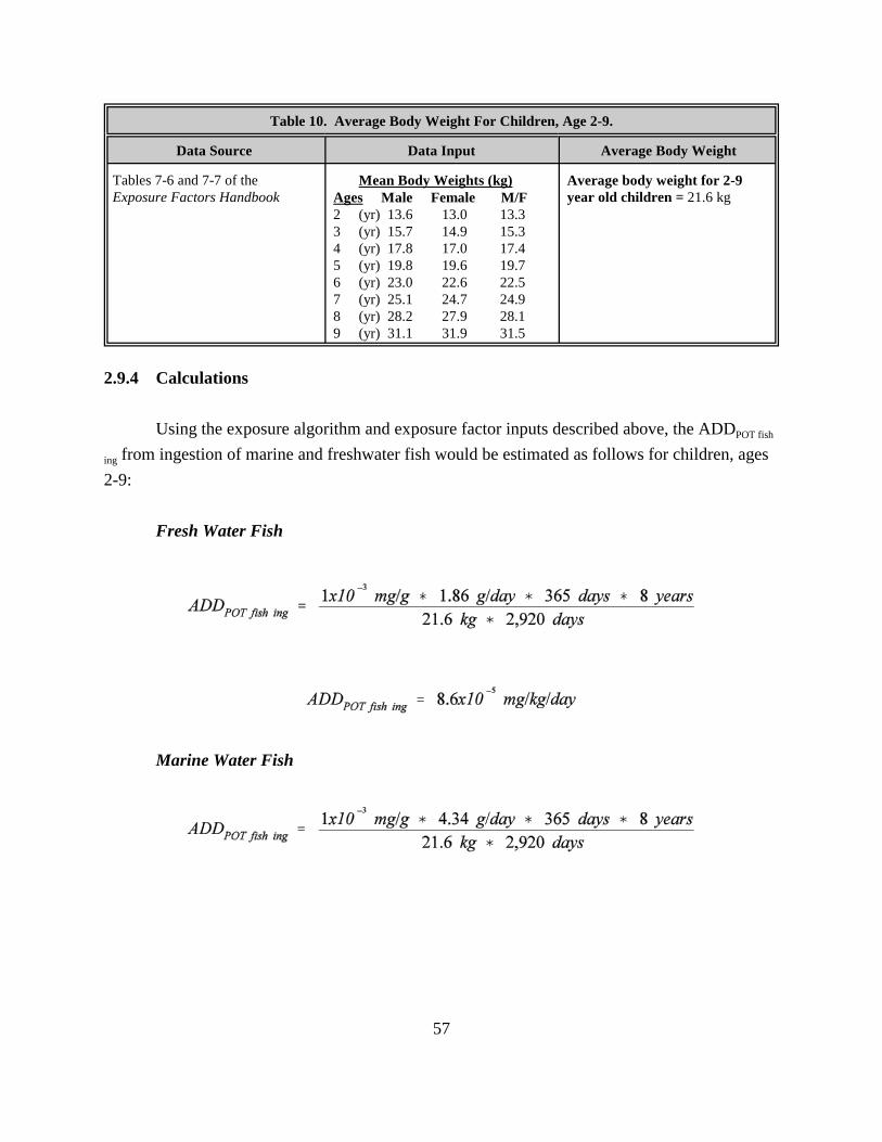
Table 10. Average Body Weight For Children, Age 2-9.
Data Source Data Input Average Body Weight
Tables 7-6 and 7-7 of the Exposure Factors Handbook
Mean Body Weights (kg) Ages Male Female M/F 2 (yr) 13.6 13.0 13.3 3 (yr) 15.7 14.9 15.3 4 (yr) 17.8 17.0 17.4 5 (yr) 19.8 19.6 19.7 6 (yr) 23.0 22.6 22.5 7 (yr) 25.1 24.7 24.9 8 (yr) 28.2 27.9 28.1 9 (yr) 31.1 31.9 31.5
Average body weight for 2-9 year old children = 21.6 kg
2.9.4 Calculations
Using the exposure algorithm and exposure factor inputs described above, the ADDPOT fish
ing from ingestion of marine and freshwater fish would be estimated as follows for children, ages 2-9:
Fresh Water Fish
Marine Water Fish
57
2.9.5 Exposure Characterization and Uncertainties
The example presented here is used to represent central tendency exposures among children, ages 2-9 years, via consumption of contaminated marine and freshwater fish. High-end exposures may be estimated by replacing the mean intake rates with the upper-percentile values. In addition, if a bounding exposure estimate is desired, the concentration in fish may also be set to the maximum measured or modeled concentration. However, caution should be used in setting all exposure factor inputs to upper-percentile values, as the resulting exposure estimate might well exceed reasonable maximum exposures for the population of interest.
Uncertainties associated with this example scenario are related to assumed activity patterns of the receptor population and the input parameters used. First, implicit in this scenario is the assumption that children, ages 2-9 years, consume contaminated fish at an intake rate of fish specified for children, ages 0-9 years, in the Exposure Factors Handbook (U.S. EPA, 1997a) and that all of the fish consumed are obtained from the contaminated site (as an alternative, a term denoting the fraction of fish assumed to be derived from the source area could be included in the dose algorithm). Also, losses of contaminant via cooking are not assumed in this example. Thus, no term denoting the fraction of contaminant lost during cooking is included. If cooking losses can be quantified, a term may be added to the dose algorithm to address such losses. Second, a single value for the average contaminant concentration in fish is used to estimate central tendency chronic exposure. This assumes that all the fish consumed from the site contain contaminant at the average concentration. The variability in average contaminant concentration in fish might introduce some degree of uncertainty as well. In addition, some uncertainty exists regarding the exposure duration. Use of an average residence time assumes that children move away from the site of contamination after 9 years. However, it is possible that a move may occur within the same area of contamination.
The confidence in the overall central tendency exposure provided in this example is related to confidences in fish intake rates, fraction of marine or freshwater fish ingested, average residence time for the general population, and the exposure concentration. The confidence rating
58

given by the Exposure Factors Handbook (U.S. EPA, 1997a) is medium for intake rates of fish, and medium for the fraction of marine or freshwater fish ingested. If the rating for the exposure concentration is also medium, the overall confidence in the central tendency exposure estimated in this example should be at least medium.
59
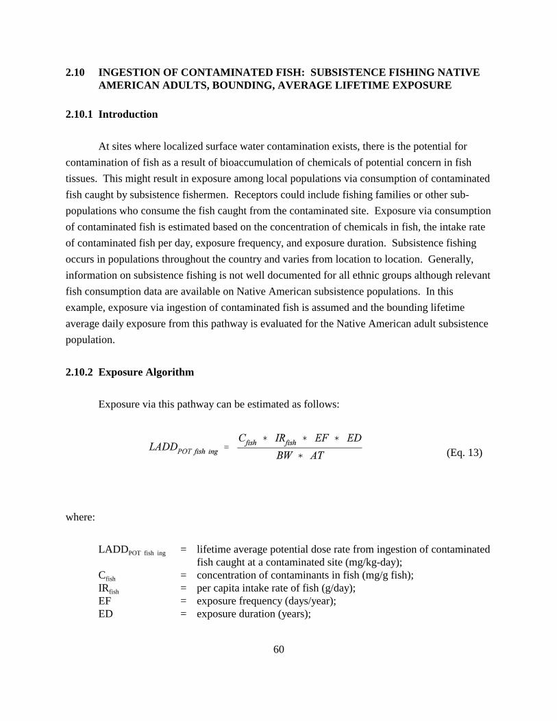
2.10 INGESTION OF CONTAMINATED FISH: SUBSISTENCE FISHING NATIVE AMERICAN ADULTS, BOUNDING, AVERAGE LIFETIME EXPOSURE
2.10.1 Introduction
At sites where localized surface water contamination exists, there is the potential for contamination of fish as a result of bioaccumulation of chemicals of potential concern in fish tissues. This might result in exposure among local populations via consumption of contaminated fish caught by subsistence fishermen. Receptors could include fishing families or other subpopulations who consume the fish caught from the contaminated site. Exposure via consumption of contaminated fish is estimated based on the concentration of chemicals in fish, the intake rate of contaminated fish per day, exposure frequency, and exposure duration. Subsistence fishing occurs in populations throughout the country and varies from location to location. Generally, information on subsistence fishing is not well documented for all ethnic groups although relevant fish consumption data are available on Native American subsistence populations. In this example, exposure via ingestion of contaminated fish is assumed and the bounding lifetime average daily exposure from this pathway is evaluated for the Native American adult subsistence population.
2.10.2 Exposure Algorithm
Exposure via this pathway can be estimated as follows:
(Eq. 13)
where:
LADDPOT fish ing = lifetime average potential dose rate from ingestion of contaminated fish caught at a contaminated site (mg/kg-day);
Cfish = concentration of contaminants in fish (mg/g fish); IRfish = per capita intake rate of fish (g/day); EF = exposure frequency (days/year); ED = exposure duration (years);
60

BW = body weight (kg); and AT = averaging time (days).
2.10.3 Exposure Factor Inputs
C fish - The concentration of contaminants in fish is either the measured or predicted concentration, based on modeling, of the chemical of interest in the fish caught in the contaminated surface water. For estimating the bounding exposure, the maximum values would be used. In this example, it is assumed that the modeled maximum concentration of chemical “x” in fish is 1x10⁻³ milligram per gram of fish (mg/g fish), as consumed.
IR fish - Intake rate of fish for the Native American adult subsistence population is provided in Table 10-72 of the Exposure Factors Handbook (U.S. EPA, 1997a). In this example, the 95th percentile of the quantity of fish consumed per day, 170 g/day, is used for the example calculation shown below.
IREF - Exposure frequency (EF) is 365 days a year because the data used in estimating
fish are assumed to represent average daily intake over the long term (i.e., over a year).
ED - Exposure duration (ED) is the length of time over which exposure occurs. In this example, 50 years is assumed. Use of this value assumes that people would consume locally caught fish for the upper-percentile residence time of 50 years (i.e., during the entire adult lifetime; between age 20 and 70 years).
AT - Since the lifetime average daily dose is being calculated in this example for an adult, the averaging time is equal to the lifetime of the individual being evaluated. The averaging time (AT) of 70 years is used for members of the general population. For use in calculations, this value is converted to 25,550 days (i.e., 70 years * 365 days/year).
BW - The average body weight of 71.8 kilograms for the general population provided in Table 7-2 of the Exposure Factors Handbook (U.S. EPA, 1997a) is used for the example calculation shown below.
61
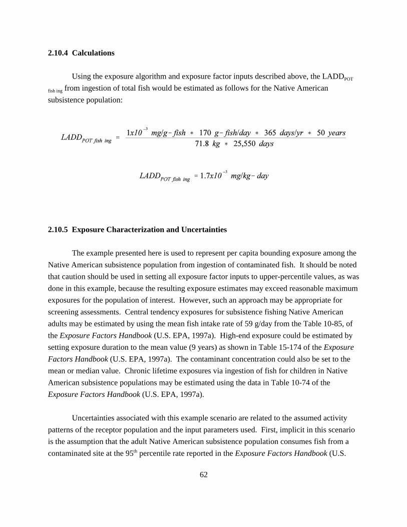
2.10.4 Calculations
Using the exposure algorithm and exposure factor inputs described above, the LADDPOT
fish ing from ingestion of total fish would be estimated as follows for the Native American subsistence population:
2.10.5 Exposure Characterization and Uncertainties
The example presented here is used to represent per capita bounding exposure among the Native American subsistence population from ingestion of contaminated fish. It should be noted that caution should be used in setting all exposure factor inputs to upper-percentile values, as was done in this example, because the resulting exposure estimates may exceed reasonable maximum exposures for the population of interest. However, such an approach may be appropriate for screening assessments. Central tendency exposures for subsistence fishing Native American adults may be estimated by using the mean fish intake rate of 59 g/day from the Table 10-85, of the Exposure Factors Handbook (U.S. EPA, 1997a). High-end exposure could be estimated by setting exposure duration to the mean value (9 years) as shown in Table 15-174 of the Exposure Factors Handbook (U.S. EPA, 1997a). The contaminant concentration could also be set to the mean or median value. Chronic lifetime exposures via ingestion of fish for children in Native American subsistence populations may be estimated using the data in Table 10-74 of the Exposure Factors Handbook (U.S. EPA, 1997a).
Uncertainties associated with this example scenario are related to the assumed activity patterns of the receptor population and the input parameters used. First, implicit in this scenario is the assumption that the adult Native American subsistence population consumes fish from a contaminated site at the 95th percentile rate reported in the Exposure Factors Handbook (U.S.
62
EPA, 1997a). This assumption requires that all Native American subsistence fishing exists on contaminated surface water and all fish consumed by the population of interest are caught from and contain contaminants from that location. Second, the ingestion rates found in the Exposure Factors Handbook (U.S. EPA, 1997a) are based on survey data from four tribes in Washington state. The example calculation assumes that the intake rates for these tribes are representative of other Native American subsistence populations found around the nation. Third, a single value for upper-percentile contaminant concentration in fish is used to estimate bounding average lifetime exposure. This assumes that the consumed fish always contains contaminant at the average concentration. The variability in average contaminant concentrations obtained from different samples might introduce some degree of uncertainty. Fourth, the exposure duration of 50 years is based on the entire adult lifetime (i.e., age 20 to 70 years). There is uncertainty as to whether the Native American population would consume fish from the contaminated location for this entire timeframe. Also, the life expectancy of Native Americans is not available, therefore data for Americans as a whole are used.
The confidence in the bounding exposure provided in this example is related to confidences in the 95th percentile fish intake rate per day, the 90th percentile residence time, and the exposure concentration. The overall confidence rating given by the Exposure Factors Handbook (U.S. EPA, 1997a) is medium for per capita intakes, but low for upper-percentiles. The rating is medium for residence time. If the rating for the exposure concentration is medium, the overall confidence rating for bounding exposure should be low to medium.
63
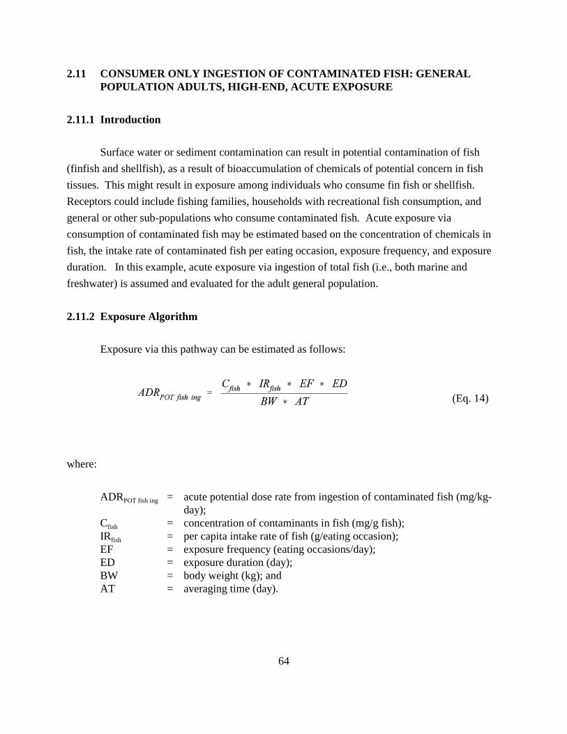
2.11 CONSUMER ONLY INGESTION OF CONTAMINATED FISH: GENERAL POPULATION ADULTS, HIGH-END, ACUTE EXPOSURE
2.11.1 Introduction
Surface water or sediment contamination can result in potential contamination of fish (finfish and shellfish), as a result of bioaccumulation of chemicals of potential concern in fish tissues. This might result in exposure among individuals who consume fin fish or shellfish. Receptors could include fishing families, households with recreational fish consumption, and general or other sub-populations who consume contaminated fish. Acute exposure via consumption of contaminated fish may be estimated based on the concentration of chemicals in fish, the intake rate of contaminated fish per eating occasion, exposure frequency, and exposure duration. In this example, acute exposure via ingestion of total fish (i.e., both marine and freshwater) is assumed and evaluated for the adult general population.
2.11.2 Exposure Algorithm
Exposure via this pathway can be estimated as follows:
(Eq. 14)
where:
ADRPOT fish ing = acute potential dose rate from ingestion of contaminated fish (mg/kg-day);
Cfish = concentration of contaminants in fish (mg/g fish); IRfish = per capita intake rate of fish (g/eating occasion); EF = exposure frequency (eating occasions/day); ED = exposure duration (day); BW = body weight (kg); and AT = averaging time (day).
64
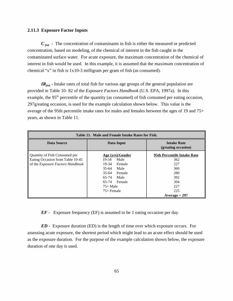
2.11.3 Exposure Factor Inputs
C fish - The concentration of contaminants in fish is either the measured or predicted concentration, based on modeling, of the chemical of interest in the fish caught in the contaminated surface water. For acute exposure, the maximum concentration of the chemical of interest in fish would be used. In this example, it is assumed that the maximum concentration of chemical “x” in fish is 1x10⁻³ milligram per gram of fish (as consumed).
IRfish - Intake rates of total fish for various age groups of the general population are provided in Table 10- 82 of the Exposure Factors Handbook (U.S. EPA, 1997a). In this example, the 95th percentile of the quantity (as consumed) of fish consumed per eating occasion, 297g/eating occasion, is used for the example calculation shown below. This value is the average of the 95th percentile intake rates for males and females between the ages of 19 and 75+ years, as shown in Table 11.
Table 11. Male and Female Intake Rates for Fish.
Data Source Data Input Intake Rate (g/eating occasion)
Quantity of Fish Consumed per Eating Occasion from Table 10-45 of the Exposure Factors Handbook
Age (yrs)/Gender 19-34 Male
19-34 Female 35-64 Male 35-64 Female 65-74 Male 65-74 Female 75+ Male 75+ Female
95th Percentile Intake Rate 362 227 360 280 392 304 227 225
Average = 297
EF - Exposure frequency (EF) is assumed to be 1 eating occasion per day.
ED - Exposure duration (ED) is the length of time over which exposure occurs. For assessing acute exposure, the shortest period which might lead to an acute effect should be used as the exposure duration. For the purpose of the example calculation shown below, the exposure duration of one day is used.
65

AT - For acute exposure assessment, averaging time is equal to exposure duration. Thus, the averaging time of one day is used in this example.
BW - Although Table 7-2 of the Exposure Factors Handbook (U.S. EPA, 1997a) shows a value of 71.8 kg for adults, an average body weight of 70 kilograms for the adult general population is used for the example calculation shown below for consistency with toxicity data.
2.11.4 Calculations
Using the exposure algorithm and exposure factor inputs shown below, the LADDPOT fish
ing from ingestion of total fish would be estimated as follows for the general population:
2.11.5 Exposure Characterization and Uncertainties
The example presented here is used to represent high-end acute exposure among general population adults from ingestion of contaminated fish. Central tendency exposures may be estimated by using the mean or median fish intake rate from Table 11.
Uncertainties associated with this example scenario are related to the assumed activity patterns of the receptor population and the input parameters used. First, implicit in this scenario is the assumption that the general population consumes contaminated fish at the 95th percentile as reported in the Exposure Factors Handbook (U.S. EPA, 1997a). Second, the ingestion intake rates for a single eating occasion found in the Exposure Factors Handbook (U.S. EPA, 1997a) are derived from data collected in 1977/78 and may not reflect recent changes in eating habits. Thus, there is some degree of uncertainty in using these intake rates to estimate exposures. Also,
66

a single value for the average contaminant concentration in fish is assumed. This assumes that all the fish consumed contain the contaminant of interest at the average concentration.
The confidence in the acute exposure provided in this example is related to confidences in the 95th percentile fish intake rate per eating occasion and the exposure concentration. A confidence rating for the amount of fish consumed per eating occasion is not given in the Exposure Factors Handbook (U.S. EPA, 1997a). However, the confidence is assumed to be medium because although it is based on a large national survey, the data are from 1977-78 and may not accurately reflect current eating patterns. If the rating for the exposure concentration is medium or higher, the overall confidence rating for acute exposure should be at least medium.
67

2.12 INGESTION OF CONTAMINATED BREAST MILK: INFANTS, CENTRAL TENDENCY SUBCHRONIC EXPOSURE
2.12.1 Introduction
Some contaminants (i.e., lipophilic compounds) can become sequestered in human breast milk and can be passed on to nursing infants via breastfeeding. Nursing mothers can take up contaminants from air, water, and locally produced food and pass them on to their nursing infants, and may have accumulated contaminant loads in adipose tissue over their lifetime. Breast-feeding infants up to 6 months of age typically obtain most of their dietary intake from breast milk. Because lipophilic contaminants are the most likely to be transferred through breast milk, the lipid content of breast milk must be considered. Receptors could include infants who are fully or partially breast fed. Exposure via ingestion of contaminated breast milk is estimated based on the concentration of contaminants in breast milk, intake rates of breast milk, exposure frequency, and exposure duration. In this example, exposure via ingestion of contaminated breast milk is assumed and the central tendency subchronic daily exposure from this pathway is evaluated for the population of infants who are fully breast fed for six months after birth.
2.12.2 Exposure Algorithm
Exposure via this pathway would be calculated as follows:
(Eq. 15)
where:
C
ADDPOT breast milk ing = potential subchronic average daily dose from ingestion of contaminated breast milk (mg/kg-day);
breast milk = concentration of contaminants in contaminated breast milk (mg/g
IR
lipid);FC = fat content or lipid content in breast milk (g lipid/g milk)
breast milk = intake rate of breast milk for infants who are fully breast fed (gmilk/kg-day);
EF = exposure frequency (days/month);ED = exposure duration (months); and
68
AT = averaging time (days).
2.12.3 Exposure Factor Inputs
Cbreast milk - The concentration of contaminants in breast milk is either the measured or predicted concentration, based on modeling, of the chemical of interest in breast milk. For estimating central tendency exposures, the mean or median values would be used. The 95% upper confidence limit of the mean concentration can be used as a conservative estimate of the mean concentration. For the purpose of the example calculations shown below, it is assumed that the modeled 95% upper confidence limit of the mean concentration of chemical “x” in breast milk is 1x10⁻³ mg/g lipid.
FC - The average fat content of breast milk is used to convert the unit of concentration from mg/g lipid to mg/g breast milk. The purpose is to ensure consistency between the units for concentration and intake rate of breast milk. Table 14-9 of the Exposure Factors Handbook (U.S. EPA, 1997a) provides data on the lipid content of breast milk of mothers who nurse infants at different months after child birth. In this example, the average lipid content of 0.04 g lipid/g milk, as recommended in Table 14-16 of the Exposure Factors Handbook (U.S. EPA, 1997a), is used.
IRbreast milk - The average intake rate of breast milk for infants from birth to 6 months of age can be estimated based on intake rates of breast milk for infants (1-12 months) provided in Table 14-15 of the Exposure Factors Handbook (U.S. EPA, 1997a). The intake rates provided in Table 14-15 are not on the basis of body weight. Thus, the intake rates in units of mL/day for 1 month, 3 month, and 6 month old infants are first converted to the intake rates in units of mL/kg-day by dividing by the average body weights for corresponding age groups of infants provided in Table 7-1 of the Exposure Factors Handbook (U.S. EPA, 1997a). The resulting intake rates are then averaged to yield the average intake rate for infants from birth to six months of age. The detailed calculations are summarized in the table below. The average breast milk intake rate of 135 mL/kg-day, as estimated, is converted to g/kg-day using the human milk density factor of 1.03 g/mL. Thus, the intake rate becomes 139 g/kg-day and is used for the example calculation shown below.
69

Table 12. Breast Milk Intake Rates.
Data Source Input Data Intake rates
Table 14-15 of the Exposure Factors Handbook
Ages Breast milk intake rate 1 month 702 mL/day 3 month 759 mL/day 6 month 765 mL/day
Ages Breast Milk Intake Rate 1 month 169.6 mL/kg-day 3 month 133.4 mL/kg-day 6 month 101.6 mL/kg-day
Average for 135 mL/kg-day 1-6 months
135 mL/day x 1.03 g/mL (human milk density factor) = 139 g/kg-day
Table 7-1 of the Exposure Factors Handbook
Ages Mean body weight (kg) Girl Boy Girl/Boy
1 month 3.98 4.29 4.14 3 month 5.40 5.98 5.69 6 month 7.21 7.85 7.53
EF - Exposure frequency is 30 days per month.
ED - Exposure duration is the length of time over which exposure occurs. For the purposes of this example, it is assumed that infants are breast fed for only six months. After that time, infants either switch to breast milk substitutes or solid food. Thus, the exposure duration of six months is used in this example.
AT - Because the subchronic average daily dose is being calculated in this example, the averaging time (AT) is equivalent to the exposure duration. Thus, AT is 6 months. This value is converted to 180 days (i.e., 6 months * 30 days/month) for the purposes of the calculations.
2.12.4 Calculations
Using the exposure algorithm and exposure factors shown above, the ADDPOT breast milk ing
is estimated as follows for the population of infants who are breast fed.
70

2.12.5 Exposure Characterization and Uncertainties
The example presented here is used to represent central tendency exposure among the population of infants who are fully breast fed for six months after birth by nursing mothers with contaminated breast milk. High-end exposures may be estimated using upper-percentile intake rates from the table cited above. If a bounding exposure estimate is desired, the concentration of contaminant may also be set to the maximum measured or modeled concentration. Caution should be used, however, in setting all exposure factor inputs to upper-percentile values, as the resulting exposure estimates may exceed reasonable maximum exposures for the population of interest.
The uncertainties associated with this example scenario are related to the assumed activity pattern of the receptor population and the input parameters used. The assumption made in this scenario is that the population of infants are breast fed for six months at the average intake rates of breast milk specified in the Exposure Factors Handbook (U.S. EPA, 1997a). In reality, the Mothers Survey (Ross Laboratories, 1999) found that 30.7% of mothers who began breast feeding in the hospital were still breast feeding at 6 months of infant age and 17.1% were still breast feeding at 12 months of age. Thus, it is possible that the exposure estimates based on an assumed exposure duration of 6 months would overestimate the actual exposure for most breast-fed infants if a lifetime average daily dose were to be calculated. There are three types of uncertainty associated with the intake rates used in this scenario. First, the intake rates may not represent the nationwide average intake rates for the population of interest due to the relatively small size of the sample used. These data may not accurately reflect the range of intra- and inter-individual variability intake over time among infants in the United States. Second, the distribution of the average intake rates generated using short-term (1-3 days) data might not reflect the long-term distribution of the average daily intakes. Thus, there would be some degree of uncertainty in using the upper-percentiles of the long-term distribution of intake rates to estimate high-end exposures. Third, the use of average body weights in conjunction with these intake rates contributes to the uncertainty since these were not the actual body weights for the infants from which the intake rates were derived. An additional source of uncertainty includes the fact that a single value for the average contaminant concentration in breast milk is used to estimate the central tendency subchronic exposure. This assumes that all the breast milk from the population of interest contains a contaminant at the average concentration. The variability in average contaminant concentrations obtained from different samples might introduce some
71

degree of uncertainty. Also, this analysis assumes the surface of the breast is uncontaminated. Thus, the infants’ exposure is from breast milk only, and not contaminants present on the mother’s skin.
The confidence in the central tendency exposure provided in this example is related to confidences in average intake rates of breast milk and exposure concentrations. The confidence rating given by the Exposure Factors Handbook (U.S. EPA, 1997a) is medium for the average intake rates. If the rating for exposure concentration is also medium, the overall confidence rating for the central tendency exposure should be at least medium.
72
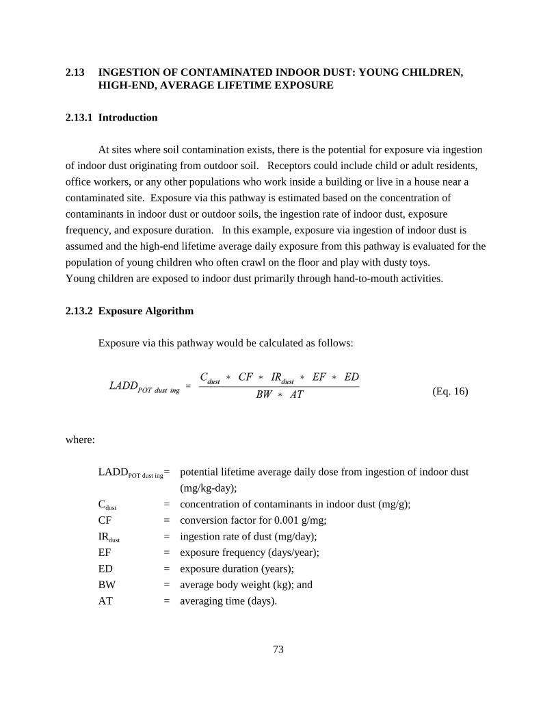
2.13 INGESTION OF CONTAMINATED INDOOR DUST: YOUNG CHILDREN, HIGH-END, AVERAGE LIFETIME EXPOSURE
2.13.1 Introduction
At sites where soil contamination exists, there is the potential for exposure via ingestion of indoor dust originating from outdoor soil. Receptors could include child or adult residents, office workers, or any other populations who work inside a building or live in a house near a contaminated site. Exposure via this pathway is estimated based on the concentration of contaminants in indoor dust or outdoor soils, the ingestion rate of indoor dust, exposure frequency, and exposure duration. In this example, exposure via ingestion of indoor dust is assumed and the high-end lifetime average daily exposure from this pathway is evaluated for the population of young children who often crawl on the floor and play with dusty toys. Young children are exposed to indoor dust primarily through hand-to-mouth activities.
2.13.2 Exposure Algorithm
Exposure via this pathway would be calculated as follows:
(Eq. 16)
where:
LADDPOT dust ing = potential lifetime average daily dose from ingestion of indoor dust (mg/kg-day);
Cdust = concentration of contaminants in indoor dust (mg/g); CF = conversion factor for 0.001 g/mg; IRdust = ingestion rate of dust (mg/day); EF = exposure frequency (days/year); ED = exposure duration (years); BW = average body weight (kg); and AT = averaging time (days).
73

2.13.3 Exposure Factor Inputs
Cdust - The concentration of contaminants in indoor dust is either the measured or predicted concentration, based on modeling, of the chemical of interest in indoor dust or outdoor soil at the contaminated site. For estimating central tendency exposures, the mean or median values would be used. The 95% upper confidence limit of the mean concentration can be used as a conservative estimate of the mean concentration. In this example, it is assumed that the modeled 95% upper confidence limit of the mean concentration of chemical “x” in indoor dust is 1x10⁻³ mg/g.
CF - A conversion factor is required to convert between mg and g.
IRdust - The upper-percentile intake rate of indoor dust for young children (1-5 years old) is calculated as the difference between the upper-percentile soil and dust ingestion rate (587 mg/day) and the upper-percentile soil ingestion rate (383 mg/day) in Table 4-22 of the Exposure Factors Handbook (U.S. EPA, 1997a). The indoor dust intake rate of 200 mg/day, as estimated, is used for the example calculation shown below.
EF - Exposure frequency is assumed to be 350 days a year for this example, because the indoor dust intake rate provided in the Table 4-22 of the Exposure Factors Handbook (U.S. EPA, 1997a) is the annual average intake rate. Young children are assumed to be away from the indoor source of contamination (e.g., on vacation) for 2 weeks per year.
ED - In this example, an exposure duration of 5 years (from age 1 to age 5) is used, based on the assumption that after 5 years of age, children no longer crawl on the floor and their indoor dust ingestion is limited compared to that of younger children.
BW - The average body weight for children between the ages of 1 and 5 years can be estimated by averaging the age-specific average body weights for children of ages 1, 2, 3, 4, and 5 provided in Table 7-3 of the Exposure Factors Handbook (U.S. EPA, 1997a). The average body weight for 1-5 year old children of 15.7 kilograms, as estimated, is used for the example calculation shown below.
AT - Because the lifetime average daily dose is being calculated in this example for a member of the general population, the averaging time (AT) is equivalent to the lifetime of the
74

individual being evaluated. The averaging time (AT) of 70 years is used for a member of the general population. For use in the calculations, this value is converted to 25,550 days (i.e., 70 years * 365 days/year).
2.13.4 Calculations
Using the exposure algorithm and exposure factors shown above, the LADDPOT dust ing is estimated as follows for the population of young children:
2.13.5 Exposure Characterization and Uncertainties
The example presented here is used to represent high-end exposure among a population of young children, ages 1-5, via ingestion of indoor dust. Central tendency exposures may be estimated using mean indoor dust intake rates. If a bounding exposure estimate is desired, the concentration of contaminants may also be set to the maximum measured or modeled concentration. Caution should be used, however, in setting all exposure factor inputs to high-end values, as the resulting exposure estimates may exceed reasonable maximum exposures for the population of interest.
The uncertainties associated with this example scenario are mainly related to the following assumed activity patterns of the receptor population and the input parameters used. First, implicit in this scenario is that young children of ages 1 to 5 ingest indoor dust at the same intake rate specified in the Exposure Factors Handbook (U.S. EPA, 1997a). It should be noted that intake rates might decrease as activity patterns change with increased ages. Second, the annual average intake rate of indoor dust for young children provided in the Exposure Factors Handbook (U.S. EPA, 1997a) is calculated based on the intake rates for both soil and dust
75
combined and soil alone. These data are derived from data collected from a variety of studies, rather than from data collected from a specific study on indoor dust. The uncertainty for the exposure estimate in this example is expected to be high for three reasons: 1) the uncertainty of estimates of soil/dust ingestion which tends to increase with upper percentile estimates; 2) the uncertainty associated with the attribution of ingestion of soil versus indoor dust; and 3) as noted in Table 4-22, “The ingestion rate studies were of short duration and are not estimates of usual intake.” For a more reliable exposure estimate, a study would need to be conducted to specifically estimate the indoor dust intake rate for young children.
The confidence in the high-end exposure estimate provided in this example is related to confidences in the upper-percentile intake rate of indoor dust and the exposure concentration. No confidence rating for indoor dust intake rate is given in the Exposure Factors Handbook (U.S. EPA, 1997a). Considering the fact that the annual average indoor dust intake rate is calculated based on the differences in soil intake rates and soil/dust intake rates from a variety of studies, rather than the data collected from a specific study, the confidence rating is expected to be low. Thus, even if the confidence rating for the exposure concentration is medium or higher, the overall confidence rating for the central tendency exposure is expected to be low.
76

2.14 INGESTION OF INDOOR DUST ORIGINATING FROM OUTDOOR SOIL: OCCUPATIONAL ADULTS, CENTRAL TENDENCY, AVERAGE LIFETIME EXPOSURE
2.14.1 Introduction
At sites where soil contamination exists, there is the potential for the transfer of contaminated soil to indoor locations, and subsequent occupational exposure via ingestion of indoor dust that adheres to food, cigarettes, or hands. Receptors could include administrative workers, or any other populations who work indoors at a site where soil contamination exists. Exposure via this pathway is estimated based on the concentration of contaminants in soils, soil ingestion rate, exposure frequency, and exposure duration. In this example, exposure via ingestion of contaminated indoor dust is assumed and the central tendency lifetime average daily exposure from this pathway is evaluated for an adult population (i.e., administrative workers).
2.14.2 Exposure Algorithm
Exposure via this pathway would be calculated as follows:
where:
=LADDPOT soil ing
=Csoil CF =
=IRsoil EF = ED = BW = AT =
(Eq. 17)
potential lifetime average daily dose from ingestion of contaminatedsoil (mg/kg-day);concentration of contaminants in soil (mg/g);conversion factor for 0.001g/mg;rate of soil ingestion (mg/day);exposure frequency (days/year);exposure duration (years);average body weight (kg); andaveraging time (days).
77
2.14.3 Exposure Factor Inputs
Csoil - The concentration of contaminants in soil is either the measured or predicted concentration, based on modeling, of the chemical of interest in the soil at a contaminated site. For estimating central tendency exposures, the mean or median values would be used. The 95% upper confidence limit of the mean concentration can be used as a conservative estimate of the mean concentration. For the purpose of the example calculations shown below, it is assumed that the modeled 95% upper confidence limit of the mean concentration of chemical “x” in soil is 1x10⁻³ mg/g.
IRsoil - According to Table 4-23 of the Exposure Factors Handbook (U.S. EPA, 1997a), the recommended average soil intake rate for adults is 50 mg/day.
EF - Exposure frequency is assumed to be 350 days a year for this example, as the soil intake rate provided in the Table 4-23 of the Exposure Factors Handbook (U.S. EPA, 1997a) is the annual average intake rate. Individuals are assumed to be away from the contaminated source (e.g., on vacation) for 2 weeks per year.
ED - Exposure duration is the length of time over which exposure occurs. For the purposes of this example, the occupational tenure of 39.8 years for the 65+ age group of individuals categorized in administrative occupations in Table 15-161 of the Exposure Factors Handbook (U.S. EPA, 1997a) is assumed.
BW - Although Table 7-2 of the Exposure Factors Handbook (U.S. EPA, 1997a) shows a value of 71.8 kg for adults, an average body weight of 70 kilograms for the adult general population is used for the example calculation shown below for consistency with toxicity data.
AT - Because the lifetime average daily dose is being calculated in this example for a member of the general population, the averaging time (AT) is equivalent to the lifetime of the individual being evaluated. The averaging time (AT) of 70 years is used for a member of the general population. For use in the calculations, this value is converted to 25,550 days (i.e., 70 years * 365 days/year).
78

2.14.4 Calculations
Using the exposure algorithm and exposure factors shown above, the LADDPOT soil ing is estimated as follows for the individuals categorized in administrative occupations:
2.14.5 Exposure Characterization and Uncertainties
The example presented here is used to represent central tendency exposure among a population of administrative workers via ingestion of indoor dust originating from contaminated soil. If a bounding exposure estimate is desired, the concentration of contaminants may be set to the maximum measured or modeled concentration. Caution should be used, however, in setting all exposure factor inputs to upper-percentile values, as the resulting exposure estimates may exceed reasonable maximum exposures for the population of interest.
The uncertainties associated with this example scenario are mainly related to the annual average intake rate of soils for adults provided in the Exposure Factors Handbook (U.S. EPA, 1997a), which is based on a limited data set for adults. Thus, the uncertainty for the exposure estimate in this example is high. For a more reliable exposure estimate, a study needs to be conducted to estimate the soil intake rate for adults who work outdoors. Another uncertainty for this scenario is the representativeness of the soil contaminant concentration to characterize inadvertent soil ingestion of soil particles adhered to food or hands. This is often addressed by using sieved soil samples to characterize the finer particles that are more likely to be adhered and subsequently ingested (U.S. EPA Technical Review Workgroup for Lead, 2000c). Soil particle size was initially explored by (Calabrese, Stanek et al., 1996) and (Stanek, Calabrese et al., 1999). Additionally, most of the soil ingestion studies did not adequately address exposure to house (indoor) dusts.
79

The confidence in the central tendency exposure estimate provided in this example is related to confidences in the average intake rate of soils, the occupational tenure for administrative workers, and the exposure concentration. The confidence rating given by the Exposure Factors Handbook (U.S. EPA, 1997a) is high for the administrative worker occupational tenure. No confidence rating for soil intake rate is given in the Exposure Factors Handbook (U.S. EPA, 1997a). Considering the fact that the annual average soil intake rate is based on limited data, the confidence rating is expected to be low. Thus, even if the confidence rating for the exposure concentration is medium or higher, the overall confidence rating for the central tendency exposure is expected to be low.
80

3.0 EXAMPLE INHALATION EXPOSURE SCENARIOS
The exposure to a chemical from the inhalation pathway is not a simple function of the inhalation rate and body weight. The physicochemical characteristics of the inhaled agent are key determinants to its interaction with the respiratory tract and ultimate deposition. Current EPA methodology uses the principles of inhalation dosimetry to determine the human equivalent concentration (HEC) for calculating a Reference Concentration (RfC) or Inhalation Unit Risk (IUR). According to these procedures, it is unnecessary to calculate inhaled dose when using dose-response factors from the Integrated Risk Information System (IRIS) in a risk assessment. Inhalation risk assessments require only an average air concentration adjusted to continuous exposure to evaluate health concerns:
• For non-carcinogens, IRIS uses Reference Concentrations (RfC) which are expressed in concentration units. Hazard is evaluated by comparing the measured or modeled concentration of the chemical in the inspired air adjusted to continuous exposure to the RfC.
• For carcinogens, IRIS uses unit risk values which are expressed in inverse concentration units. Risk is evaluated by multiplying the unit risk by the measured or modeled concentration of the chemical in the inspired air adjusted to continuous exposure.
Exposure information, specifically information related to activity patterns (e.g., exposure time, frequency, and duration, as well as contaminant concentration) may vary across age groups and other population groups. Consequently, such variation should be taken into account in deriving both lifetime excess cancer risk and hazard quotient estimates. Beyond the consideration of time spent in the area of contamination and any change in concentration of the contaminant in that area, no additional corrections to the risk calculations for specific age groups are necessary. The exposure scenarios presented in the sections that follow show how these adjustments in concentration are applied to various populations.
81

3.1 INHALATION OF CONTAMINATED INDOOR AIR: OCCUPATIONAL FEMALE ADULTS, CENTRAL TENDENCY, AVERAGE LIFETIME EXPOSURE
3.1.1 Introduction
At sites where the use of occupationally related chemical products results in indoor air contamination, there may be a potential for occupational exposure via inhalation. Receptors could include commercial/ industrial workers, doctors and nurses, or any population who inhales contaminated air as a result of their occupation.
3.1.2 Exposure Algorithm
The equations in the sections below provide the appropriate equations for calculating the concentration of the chemical in the inspired air adjusted to continuous exposure that can be used directly in the risk assessment.
(Eq. 18)
where:
Cindoor air (adjusted) Cindoor air
= =
concentration of contaminants in indoor air adjusted (mg/m3); concentration of contaminants in indoor air (mg/m3);
ET = exposure time (hr/day); EF = exposure frequency (days/year); ED = exposure duration (years); and AT = averaging time (hours).
3.1.3 Exposure Factor Inputs
Cindoorair - The concentration of contaminants in air is either the measured or predicted concentration, based on modeling, of the chemical of interest in the air at the site of interest. For estimating central tendency exposures, the mean or median values would be used. The 95% upper confidence limit of the mean concentration can be used as a conservative estimate of the mean
82
concentration. For the purpose of the example calculations shown below, it is assumed that the modeled 95 percent upper confidence limit of the mean concentration of chemical “x” in air is 1x10⁻³ mg/m3.
ET- Exposure time is 8 hours/day, as female nurses are assumed to work eight hours per day in this example. It should be noted that site-specific values may be used if available. For example, some hospitals require that nurses work shifts (e.g., 12 hour shifts) over fewer days (e.g., 3 days/week). Note that these alternate exposure times and frequencies would result in exposure estimates that closely resemble those provided in this example.
EF - Exposure frequency is assumed to be 219 days a year for this example. This estimate assumes that female nurses work 5 days a week, observe 10 Federal holidays, take 4 weeks of vacation a year and an additional 12 personal days. This value is recommended by U.S. EPA (1989) to represent central tendency exposure frequency for industrial/technical workers.
ED - Exposure duration is the length of time over which exposure occurs. For the purposes of this example, the occupational tenure of 22.2 years for the 65+ age group of Technicians and Related Support provided in Table 15-161 of the Exposure Factors Handbook (U.S. EPA, 1997a) is assumed. This value assumes that female nurses inhaled occupationally related contaminated air in a hospital for the occupational tenure of 22.2 years. After that time, female nurses at the ages of 65+ are assumed to be retired and no longer inhale the contaminated air.
AT - Because the lifetime average daily exposure for a member of the general female population is of interest in this example, the averaging time (AT) is equivalent to the lifetime of the individual being evaluated. According to Section 8.2 of the Exposure Factors Handbook (U.S. EPA, 1997a), the averaging time (AT) of 70 years is recommended for a member of the general population. For use in the calculations, this value is converted to 613,200 hours (i.e., 70 years * 365 days/year * 24 hours/day).
3.1.4 Calculations
Using the exposure factors shown above and equation 18, the C indoor air adjusted is estimated as follows:
83

3.1.5 Exposure Characterization and Uncertainties
The example presented here is used to represent central tendency occupational exposure among the population of female nurses who inhale certain work-related chemicals. High-end exposures may be estimated by increasing the exposure time, frequency, and duration. If a bounding exposure estimate is desired, the concentration of contaminants may be set to the maximum measured or modeled concentration. Caution should be used, however, in setting all exposure factor inputs to high-end values, as the resulting exposure estimates may exceed reasonable maximum exposures for the population of interest.
The uncertainties associated with this example scenario are related to the assumed activity pattern of the receptor population and the input parameters used. The assumption of a 5-day work week introduces some uncertainty since this may not reflect the shift approach employed by certain hospitals. The specific working hours employed by the workers being assessed should be used in calculating the exposure scenario. The assumption of retirement age may introduce some uncertainty also and may vary for different receptor populations.
The confidence in the central tendency exposure estimate provided in this example is related to confidences in an assumed activity pattern, occupational tenure, and exposure concentrations. The confidence rating given by the Exposure Factors Handbook (U.S. EPA, 1997a) is high for the occupational tenure. Thus, if the confidence rating is medium for the assumed activity pattern and medium for the exposure concentration, the overall confidence rating for the central tendency exposure is at least medium.
84

3.2 INHALATION OF CONTAMINATED INDOOR AIR: RESIDENTIAL CHILD, CENTRAL TENDENCY, AVERAGE LIFETIME EXPOSURE
3.2.1 Introduction
At sites where localized volatile contaminants intrude into residences or where the use of commercial products or other materials results in indoor air contamination, there may be the potential for exposure among residents via inhalation. In this example, exposure via inhalation of contaminated indoor air is assumed and the central tendency lifetime average daily exposure from this pathway is evaluated for the residential child (ages 3-11 years).
3.2.2 Exposure Algorithm
The adjusted indoor air concentration (C indoor air adjusted ) is estimated as follows:
(Eq. 19)
where:
CCindoor air (adjusted) = concentration of contaminants in indoor air adjusted (mg/m3);
indoor air = concentration of contaminants in indoor air (mg/m3);ET = exposure time (hr/day);EF = exposure frequency (days/year);ED = exposure duration (years); andAT = averaging time (hours).
3.2.3 Exposure Factor Inputs
Cindoor air - The concentration of contaminants in air is either the measured or predicted concentration, based on modeling, of the chemical of interest in the air at the site of interest. For estimating central tendency exposures, the mean or median values would be used. The 95% upper confidence limit of the mean concentration can be used as a conservative estimate of the mean concentration. For the purpose of the example calculations shown below, it is assumed that the
85
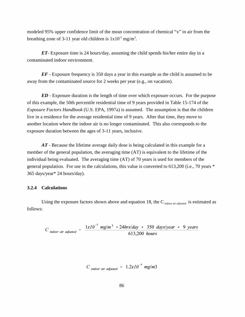
modeled 95% upper confidence limit of the mean concentration of chemical “x” in air from the breathing zone of 3-11 year old children is 1x10⁻³ mg/m3.
ET- Exposure time is 24 hours/day, assuming the child spends his/her entire day in a contaminated indoor environment.
EF - Exposure frequency is 350 days a year in this example as the child is assumed to be away from the contaminated source for 2 weeks per year (e.g., on vacation).
ED - Exposure duration is the length of time over which exposure occurs. For the purpose of this example, the 50th percentile residential time of 9 years provided in Table 15-174 of the Exposure Factors Handbook (U.S. EPA, 1997a) is assumed. The assumption is that the children live in a residence for the average residential time of 9 years. After that time, they move to another location where the indoor air is no longer contaminated. This also corresponds to the exposure duration between the ages of 3-11 years, inclusive.
AT - Because the lifetime average daily dose is being calculated in this example for a member of the general population, the averaging time (AT) is equivalent to the lifetime of the individual being evaluated. The averaging time (AT) of 70 years is used for members of the general population. For use in the calculations, this value is converted to 613,200 (i.e., 70 years * 365 days/year* 24 hours/day).
3.2.4 Calculations
Using the exposure factors shown above and equation 18, the C indoor air adjusted is estimated as follows:
86

3.2.5 Exposure Characterization and Uncertainties
The example presented here is used to represent central tendency exposure among residential children from inhalation of contaminated indoor air. High-end exposures may be estimated by using the upper-percentile values for the residence time. If a bounding exposure estimate is desired, the concentration of contaminants may also be set to the maximum measured or modeled concentration.
The confidence in the central tendency exposure estimate provided in this example is related to confidences in the residential time, and exposure concentrations. The confidence rating given by the Exposure Factors Handbook (U.S. EPA, 1997a) is medium for the residence time. Thus, if the confidence rating is medium for the exposure concentration, the overall confidence rating for the central tendency exposure is at least medium.
87

3.3 INHALATION OF CONTAMINATED INDOOR AIR: SCHOOL CHILDREN, CENTRAL TENDENCY, SUBCHRONIC EXPOSURE
3.3.1 Introduction
Volatile contaminants may intrude into buildings or chemicals may volatilize from consumer products or other materials resulting in indoor air contamination. This may result in the potential for exposure via inhalation. Receptors could include residents, commercial/industrial workers, students, recreational populations, etc. For the purposes of this example, exposure among elementary school children (i.e., 6 to 11 year olds) via inhalation of contaminated air inside a school building is assumed. Central tendency subchronic daily exposure from inhalation is evaluated for this population.
3.3.2 Exposure Algorithm
Exposure via this pathway would be calculated as follows:
(Eq. 20)
where:
Cindoor air adjusted Cindoor air
= =
concentration of contaminants in indoor air adjusted (mg/m3); concentration of contaminant in the indoor air (mg/m3);
ET = exposure time (hr/day); EF = exposure frequency (days/year); ED = exposure duration (years); and AT = averaging time (hours).
3.3.3 Exposure Factor Inputs
C indoor air - The concentration of contaminant in air at the site (Cindoor air) is either the measured or predicted concentration, based on modeling, of the chemical of interest in the air at
88
the site of interest. For estimating central tendency exposures the mean or median values would be used. Often, the 95% upper confidence limit of the mean concentration is used as a conservative estimate of the mean concentration. For the purposes of this example, it is assumed that the 95 percent upper confidence limit of the mean measured concentration of chemical “x” in air is 1x10⁻³ mg/m3.
ET - Table 15-84 of the Exposure Factors Handbook (U.S. EPA, 1997a) shows that both the median and mean number of minutes spent in school for 5 to 11 year old children is 390 minutes (i.e., 6.5 hours). Data are not specifically available for 6 to 11 year olds; therefore, the value for the 5 to 11 year old range is used for this scenario. Use of this value assumes that the children spend all of their time in the building (i.e., it does not account for time that might be spent outdoors in the playground). Thus, under certain circumstances, this value may slightly overestimate the exposure time indoors.
EF - Exposure frequency is assumed to be 185 days a year for this example. This is equivalent to 37 weeks of full-time school, and accounts for 15 weeks off for summer and winter vacation, Federal and school holidays, etc.
ED - Exposure duration is the length of time over which exposure occurs. For the purposes of this example, the exposure duration for 6 to 11 year old school children is assumed to be six years (i.e., first grade through sixth grade). This assumes that all six years are spent in the same building where indoor air contamination exists.
AT - Because the subchronic average daily dose is being calculated for a member of the general population, the averaging time is equivalent to the exposure duration. For the purposes of this example, the averaging time is converted to 52,560 hours (i.e., 6 years * 365 days/year * 24 hours/day).
3.3.4 Calculations
Using the exposure algorithm and exposure factor inputs shown above, the Cindoor air (adjusted)
for elementary school age children would be as follows:
89

3.3.5 Exposure Characterization and Uncertainties
The example presented here is used to represent central tendency exposures among the general population of elementary school children from the inhalation of contaminated air inside the school building. High-end exposures may be estimated by increasing exposure durations and frequencies. Caution should be used, however, in setting all exposure factor inputs to upper-percentile values, as the resulting exposure estimates may exceed reasonable maximum exposures for the population of interest.
The uncertainties associated with this example scenario are related to the concentrations and assumed exposure durations and frequencies. Assuming that the confidence in the exposure concentration is at least medium, confidence in the overall central tendency exposure example provided here should be at least medium.
90
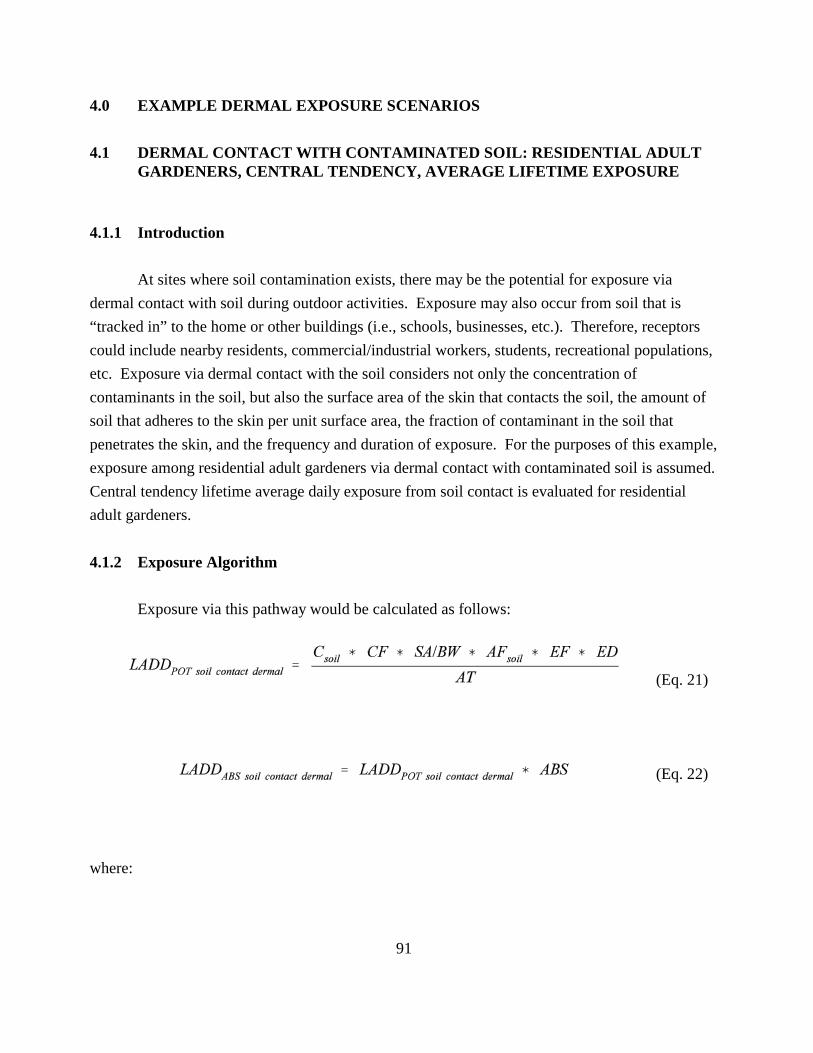
4.0 EXAMPLE DERMAL EXPOSURE SCENARIOS
4.1 DERMAL CONTACT WITH CONTAMINATED SOIL: RESIDENTIAL ADULT GARDENERS, CENTRAL TENDENCY, AVERAGE LIFETIME EXPOSURE
4.1.1 Introduction
At sites where soil contamination exists, there may be the potential for exposure via dermal contact with soil during outdoor activities. Exposure may also occur from soil that is “tracked in” to the home or other buildings (i.e., schools, businesses, etc.). Therefore, receptors could include nearby residents, commercial/industrial workers, students, recreational populations, etc. Exposure via dermal contact with the soil considers not only the concentration of contaminants in the soil, but also the surface area of the skin that contacts the soil, the amount of soil that adheres to the skin per unit surface area, the fraction of contaminant in the soil that penetrates the skin, and the frequency and duration of exposure. For the purposes of this example, exposure among residential adult gardeners via dermal contact with contaminated soil is assumed. Central tendency lifetime average daily exposure from soil contact is evaluated for residential adult gardeners.
4.1.2 Exposure Algorithm
Exposure via this pathway would be calculated as follows:
(Eq. 21)
(Eq. 22)
where:
91

LADDPOT soil contact dermal = potential lifetime average daily dose from dermal contact with contaminated soil (mg/kg-day);
LADDABS soil contact dermal = absorbed lifetime average daily dose from dermal contact with contaminated soil (mg/kg-day);
Csoil = concentration of contaminant in the soil at the
CF = site (mg/kg); conversion factor (1x10⁻⁶ kg/mg);
SA/BW
AFsoil
=
=
surface area of the skin that contacts the soil (cm2/event) divided by body weight (kg); adherence factor for soil (mg/cm2);
EF = exposure frequency (events/year); ED = exposure duration (years); ABS = absorption fraction; this value is chemical-
specific; and AT = averaging time (days).
4.1.3 Exposure Factor Inputs
Csoil - The concentration of contaminant in soil at the site (Csoil) is either the measured or predicted concentration, based on modeling, of the chemical of interest in the soil at the site of interest. For estimating central tendency exposures the mean or median values would be used. Often, the 95% upper confidence limit of the mean concentration is used as a conservative estimate of the mean concentration. For the purposes of the example calculations provided below, it is assumed that the 95 % upper confidence limit of the mean measured concentration of chemical “x” in soil is 1 mg/kg.
CF - A conversion factor is required to convert between mg/kg and kg/mg. The value is 1 x 10⁻⁶ kg/mg because there are 1,000,000 mg per kg.
SA/BW - The surface area of the skin that comes into contact with the soil (SA) during each exposure event can be estimated in several ways. The three approaches described below are meant to highlight the available data in the Exposure Factors Handbook (U.S. EPA, 1997a) and to show the various ways in which these data can be used to calculate the surface area of the skin that comes in contact with the contaminated soil. One method may be preferable over the other depending on the exposure scenario being evaluated and the data available to the assessor. For
92

the first approach, an estimate of the percentage of the body exposed to soil can be made. This percentage is used in conjunction with the total surface area of the body. For the purposes of this example, it is assumed that 25 percent of the body is exposed. The total surface area of the body is assumed to be 18,150 cm2, based on the average 50th percentile surface areas for adult males (1.94 m2;19,400 cm2) and females (1.69 m2; 16,900 cm2), as cited in Table 6-4 of the Exposure Factors Handbook (U.S. EPA, 1997a). The resulting exposed surface area (SA) value is 4,540 cm2/event. This value is divided by the average body weight for male and female adults between the ages of 18 and 75 years (71.8 kg), as shown in Table 7-2 of the Exposure Factors Handbook (U.S. EPA, 1997a) to estimate a SA/BW of 63.2 cm2/event-kg. According to EPA’s Risk Assessment Guidance for Superfund (U.S. EPA, 1998b), 50th percentile surface area values should also be used for reasonable maximum exposure estimates (i.e., instead of 95th percentile surface area values), when using an average body weight, because of the strong correlation between surface area and body weights, and because 50th percentile values are “most representative of the surface areas of individuals of average weight” (U.S. EPA, 1989). A second approach is to make assumptions about the specific body parts that are expected to be exposed to soil, given the likely clothing scenario for the activity of interest. For this example scenario (i.e., gardening), it is assumed that an individual will wear short pants and short sleeve shirt, and that the hands, lower arms, and lower legs will come into contact with the soil. Using Tables 6-2 and 6-3 of the Exposure Factors Handbook (U.S. EPA, 1997a), surface area values are obtained and averaged for male and female hands and lower legs. One-half the values for arms are used to represent only the lower arms. The values for the three body parts are then summed to represent the average total exposed surface area for males and females (4,578 cm2/event), and divided by the average body weight for males and females (71.8 kg) to obtain the SA/BW value (63.8 cm2/event-kg). A third approach is to use the surface area to body weight ratio values presented in Table 6-9 of the Exposure Factors Handbook (U.S. EPA, 1997a). The data in Table 6-9 were developed by dividing the measured total surface areas for 401 individuals by their corresponding body weights and developing a distribution of SA/BWs for the study population. The advantage of using the data from this distribution is that the correlation between surface area and body weight is accounted for. Because these SA/BWs are based on total body surfaces, they are multiplied by 0.25 to estimate the surface area assumed to be exposed in this example. As shown in the following table, the estimates obtained by these three methods are similar, with a slightly higher value being obtained by Approach 3. These differences are relatively small and are not expected to significantly impact the doses estimated for this example.
93
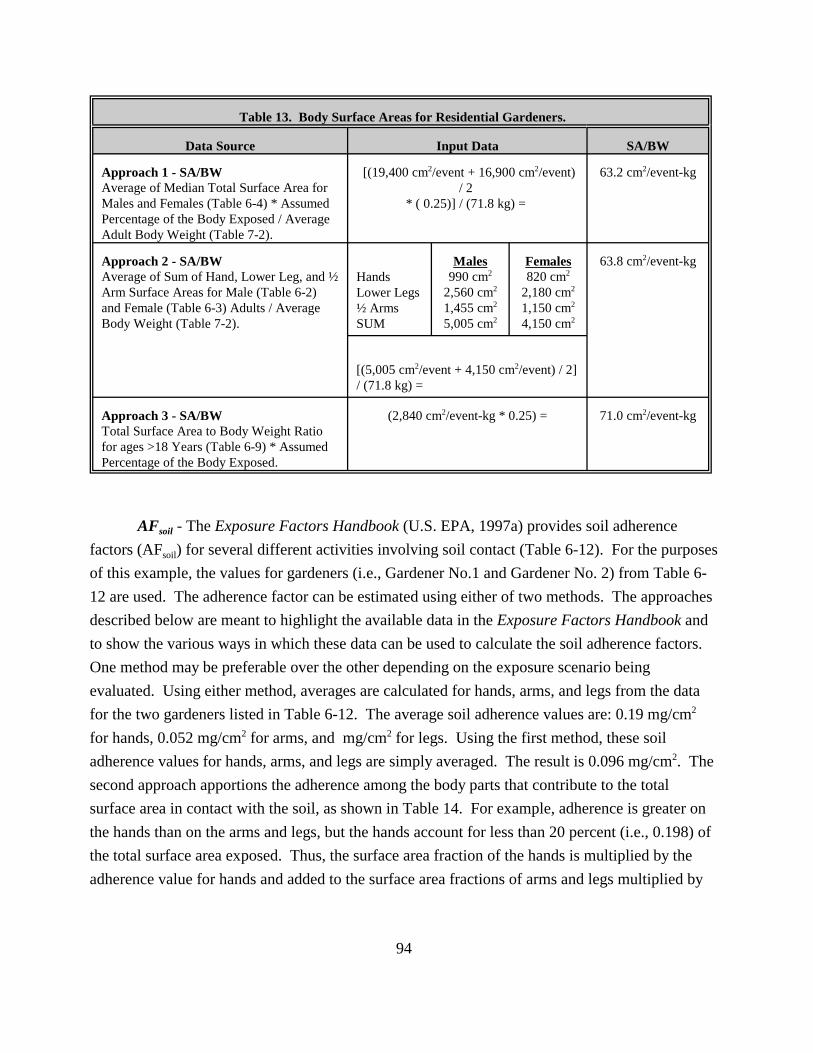
Table 13. Body Surface Areas for Residential Gardeners.
Data Source Input Data SA/BW
Approach 1 - SA/BW Average of Median Total Surface Area for Males and Females (Table 6-4) * Assumed Percentage of the Body Exposed / Average Adult Body Weight (Table 7-2).
[(19,400 cm2/event + 16,900 cm2/event) / 2
* ( 0.25)] / (71.8 kg) =
63.2 cm2/event-kg
Approach 2 - SA/BW Average of Sum of Hand, Lower Leg, and ½ Arm Surface Areas for Male (Table 6-2) and Female (Table 6-3) Adults / Average Body Weight (Table 7-2).
Hands Lower Legs ½ Arms SUM
Males 990 cm2
2,560 cm2
1,455 cm2
5,005 cm2
Females 820 cm2
2,180 cm2
1,150 cm2
4,150 cm2
63.8 cm2/event-kg
[(5,005 cm2/event + 4,150 cm2/event) / 2] / (71.8 kg) =
Approach 3 - SA/BW Total Surface Area to Body Weight Ratio for ages >18 Years (Table 6-9) * Assumed Percentage of the Body Exposed.
(2,840 cm2/event-kg * 0.25) = 71.0 cm2/event-kg
AFsoil - The Exposure Factors Handbook (U.S. EPA, 1997a) provides soil adherence factors (AFsoil) for several different activities involving soil contact (Table 6-12). For the purposes of this example, the values for gardeners (i.e., Gardener No.1 and Gardener No. 2) from Table 612 are used. The adherence factor can be estimated using either of two methods. The approaches described below are meant to highlight the available data in the Exposure Factors Handbook and to show the various ways in which these data can be used to calculate the soil adherence factors. One method may be preferable over the other depending on the exposure scenario being evaluated. Using either method, averages are calculated for hands, arms, and legs from the data for the two gardeners listed in Table 6-12. The average soil adherence values are: 0.19 mg/cm2
for hands, 0.052 mg/cm2 for arms, and mg/cm2 for legs. Using the first method, these soil adherence values for hands, arms, and legs are simply averaged. The result is 0.096 mg/cm2. The second approach apportions the adherence among the body parts that contribute to the total surface area in contact with the soil, as shown in Table 14. For example, adherence is greater on the hands than on the arms and legs, but the hands account for less than 20 percent (i.e., 0.198) of the total surface area exposed. Thus, the surface area fraction of the hands is multiplied by the adherence value for hands and added to the surface area fractions of arms and legs multiplied by
94
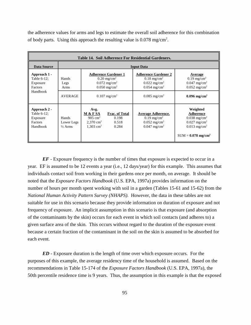
the adherence values for arms and legs to estimate the overall soil adherence for this combination of body parts. Using this approach the resulting value is 0.078 mg/cm2.
Table 14. Soil Adherence For Residential Gardeners.
Data Source Input Data
Approach 1 Table 6-12; Hands
Adherence Gardener 1 0.20 mg/cm2
Adherence Gardener 2 0.18 mg/cm2
Average 0.19 mg/cm2
Exposure Legs 0.072 mg/cm2 0.022 mg/cm2 0.047 mg/cm2
Factors Arms 0.050 mg/cm2 0.054 mg/cm2 0.052 mg/cm2
Handbook AVERAGE 0.107 mg/cm2 0.085 mg/cm2 0.096 mg/cm2
Approach 2 - Avg. Weighted Table 6-12; Exposure Hands
M & F SA Frac. of Total 905 cm2 0.198
Average Adherence. 0.19 mg/cm2
Adherence 0.038 mg/cm2
Factors Lower Legs 2,370 cm2 0.518 0.052 mg/cm2 0.027 mg/cm2
Handbook ½ Arms 1,303 cm2 0.284 0.047 mg/cm2 0.013 mg/cm2
SUM = 0.078 mg/cm2
EF - Exposure frequency is the number of times that exposure is expected to occur in a year. EF is assumed to be 12 events a year (i.e., 12 days/year) for this example. This assumes that individuals contact soil from working in their gardens once per month, on average. It should be noted that the Exposure Factors Handbook (U.S. EPA, 1997a) provides information on the number of hours per month spent working with soil in a garden (Tables 15-61 and 15-62) from the National Human Activity Pattern Survey (NHAPS). However, the data in these tables are not suitable for use in this scenario because they provide information on duration of exposure and not frequency of exposure. An implicit assumption in this scenario is that exposure (and absorption of the contaminants by the skin) occurs for each event in which soil contacts (and adheres to) a given surface area of the skin. This occurs without regard to the duration of the exposure event because a certain fraction of the contaminant in the soil on the skin is assumed to be absorbed for each event.
ED - Exposure duration is the length of time over which exposure occurs. For the purposes of this example, the average residency time of the household is assumed. Based on the recommendations in Table 15-174 of the Exposure Factors Handbook (U.S. EPA, 1997a), the 50th percentile residence time is 9 years. Thus, the assumption in this example is that the exposed
95

population contacts contaminated soil from the site at which they reside for 9 years. After that time, they are assumed to reside in a location where the soil is not affected by contamination from the site.
ABS - This value is chemical specific. Information on absorption fractions can be obtained from EPA’s Dermal Exposure Assessment: Principles and Applications (U.S. EPA, 1992b). EPA has also developed the draft Part E Supplemental Guidance for Dermal Risk Assessment of the Risk Assessment Guidance for Superfund, Volume I: Human Health Evaluation Manual (U.S. EPA, 2001b). This document provides another source of data on dermal absorption. Although this document is not final, it is generally more representative of current thinking in this area and assessors are encouraged to use it instead of U.S. EPA (1992b). For the purposes of the calculations provided below for this example, it is assumed that the absorption fraction for the chemical of interest (i.e., chemical “x”) is 0.1.
AT - Because the lifetime average daily dose is being calculated for a member of the general population, the averaging time is equivalent to the lifetime of the individual being evaluated. For the purposes of this example, the average lifetime for men and women is used because the exposures are assumed to reflect the general population and are not gender- or age-specific. The averaging time of 70 years is used in the calculations. This value is converted to 25,550 days (i.e., 70 years * 365 days/year).
4.1.4 Calculations
LADDUsing the exposure algorithm and exposure factor inputs shown above, the
ABS soil contact dermal would be as follows using either Approach 1, Approach 2, or Approach 3 for calculating SA/BW for the adults, combined with the results of Approach 2 for calculating the adherence value:
Approach 1
96

Approach 2
Approach 3
97
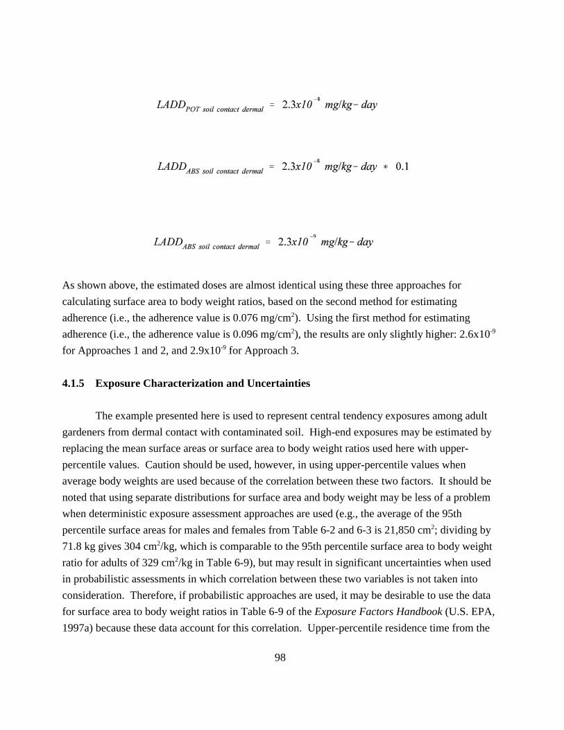
As shown above, the estimated doses are almost identical using these three approaches for calculating surface area to body weight ratios, based on the second method for estimating adherence (i.e., the adherence value is 0.076 mg/cm2). Using the first method for estimating adherence (i.e., the adherence value is 0.096 mg/cm2), the results are only slightly higher: 2.6x10⁻⁹
for Approaches 1 and 2, and 2.9x10⁻⁹ for Approach 3.
4.1.5 Exposure Characterization and Uncertainties
The example presented here is used to represent central tendency exposures among adult gardeners from dermal contact with contaminated soil. High-end exposures may be estimated by replacing the mean surface areas or surface area to body weight ratios used here with upper-percentile values. Caution should be used, however, in using upper-percentile values when average body weights are used because of the correlation between these two factors. It should be noted that using separate distributions for surface area and body weight may be less of a problem when deterministic exposure assessment approaches are used (e.g., the average of the 95th percentile surface areas for males and females from Table 6-2 and 6-3 is 21,850 cm2; dividing by 71.8 kg gives 304 cm2/kg, which is comparable to the 95th percentile surface area to body weight ratio for adults of 329 cm2/kg in Table 6-9), but may result in significant uncertainties when used in probabilistic assessments in which correlation between these two variables is not taken into consideration. Therefore, if probabilistic approaches are used, it may be desirable to use the data for surface area to body weight ratios in Table 6-9 of the Exposure Factors Handbook (U.S. EPA, 1997a) because these data account for this correlation. Upper-percentile residence time from the
98

table cited above may also be used to estimate high-end exposures. If a bounding exposure estimate is desired, the concentration in soil may be set to the maximum measured or modeled concentration, and the assumed frequency of exposure may be increased (e.g., once per day). Caution should be used, however, in setting all exposure factor inputs to upper-percentile values, as the resulting exposure estimates may exceed reasonable maximum exposures for the population of interest.
The uncertainties associated with this example scenario are related to assumed activity patterns of the receptor population and the input parameters used. Implicit in this scenario is the assumption that the population of interest contacts the contaminated soil from the site, and that adherence occurs over the assumed surface area of the skin at the rates shown in the Exposure Factors Handbook (U.S. EPA, 1997a). Another implicit assumption is that the soil is on the skin for the entire exposure event, which is assumed to be a day. This means that each event (whether it consists of a few minutes or several hours) is assumed to be one day. Multiple soil contact events in a single day are still treated as one event. Use of a one day exposure event is consistent with absorption values, which are typically based on 24-hour exposure periods. The assumption that absorption from contaminants in soil adhering to the skin occurs over 24 hours contributes to the uncertainty of the resulting estimates because it is possible that individuals may bathe. Selection of the clothing scenario or percentage of the body exposed should be based on the assessors knowledge of the populations/activities and should be designed to reflect, as closely as possible, the skin surface area exposed for the activity of interest. However, the assumptions used regarding the clothing worn and the surface area exposed results in uncertainty in the assessment. The Exposure Factors Handbook (U.S. EPA, 1997a) describes the uncertainty associated with the surface area and adherence data, and concludes that although there may be some selection bias associated with the surface area data upon which the recommended values are based, they are the best available data for use in exposure assessment. The uncertainties associated with the adherence data result from the limited size of the data set, and the fact that adherence may be influenced by the clothing worn by the study participants, and soil properties (e.g., moisture content, particle size) that are not entirely accounted for in the available data.
It should be noted that the confidence ratings given by the Exposure Factors Handbook (U.S. EPA, 1997a) are high for surface area data, but low for soil adherence data and low for the absorption fraction. Assuming that the confidence in the exposure concentration is also at least medium, confidence in the overall central tendency exposure example provided here should be low based on the soil adherence data and absorption fraction.
99

4.2 DERMAL CONTACT WITH SOIL: TEEN ATHLETE: CENTRAL TENDENCY, SUBCHRONIC EXPOSURE
4.2.1 Introduction
At sites where localized soil contamination exists, there may be the potential for exposure via dermal contact with soil during outdoor activities. Exposure may also occur from soil that is “tracked in” to the home or other buildings (i.e., schools, businesses, etc.). Therefore, receptors could include nearby residents, commercial/industrial workers, students, recreational populations, etc. Exposure via dermal contact with the soil considers not only the concentrations of contaminants in the soil, but also the surface area of the skin that contacts the soil, the amount of soil that adheres to the skin per unit surface area, the fraction of contaminant in the soil that penetrates the skin, and the frequency and duration of exposure. For the purposes of this example, exposure among teen athletes via dermal contact with contaminated soil is assumed. A subchronic average daily dermal dose from soil contact is evaluated for the teen athlete. For the purposes of this assessment a teen athlete (age 13-15 years) playing soccer for one-half of the year is evaluated.
4.2.2 Exposure Algorithm
Exposure via this pathway would be calculated as follows:
where:
ADDABS soil contact dermal =
Csoil = CF = SA/BW =
AFsoil = EF =
(Eq. 23)
absorbed average daily dose from dermal contact withcontaminated soil (mg/kg-day);concentration of contaminant in the soil at the site (mg/kg);conversion factor (1x10⁻⁶ kg/mg);surface area of the skin that contacts the soil (cm2/event)divided by body weight (kg); adherence factor for soil (mg/cm2);exposure frequency (events/yr);
100

ED = exposure duration (years); ABS = absorption fraction; this value is chemical-specific; and AT = averaging time (days).
4.2.3 Exposure Factor Inputs
Csoil - The concentration of contaminant in soil at the site (Csoil) is either the measured or predicted concentration, based on modeling, of the chemical of interest in the soil at the site of interest. In the case of a central tendency scenario, the 95% upper confidence limit of the mean concentration is used as a conservative estimate of the mean concentration. For the purposes of the example calculations provided below, it is assumed that the 95% upper confidence limit of the mean measured concentration of chemical “x” in soil is 1x10⁻³ mg/kg.
CF - A conversion factor is required to convert between mg/kg and kg/mg. The value is 1x10⁻⁶ kg/mg because there are 1,000,000 mg per kg.
SA/BW - For this assessment, assumptions will be made regarding the surface area of specific body parts that are expected to be exposed to soil. For this example scenario (i.e., teen athlete), it is assumed that an individual will wear short pants and short sleeve shirt, and that the hands, arms, and legs will come into contact with the soil. The SA/BW calculation is developed in Table 15. First, Table 6-8 of the Exposure Factors Handbook (U.S. EPA, 1997a) is used to obtain the percent surface area contribution of arms, legs, and hands to the total surface area. The percent contribution for each body part is added together to represent the total percentage of exposed skin expected for exposed hands, arms, and legs. Next, Tables 6-6 and 6-7 of the Exposure Factors Handbook (U.S. EPA, 1997a) are used to identify the 50th percentile total body surface areas for male and female children (age 13-15 years). The age group data for males and females are averaged to represent exposure to this age group. The same general procedure is used to calculate the 50th percentile body weights. Tables 7-6 and 7-7 of the Exposure Factors Handbook (U.S. EPA, 1997a) are used to identify male and female body weights for children aged 13 to 15 years.
The total surface area for children (age 13-15 years) is calculated to be 15,633 cm2 . The total surface area is multiplied by the percent ratio of exposed arms, legs and hands (49.2%) to calculate exposed surface area for males and females to obtain 7,691 cm2/event. The average
101

body weight for male and females is then divided by the average body weight for male and female children (53.2 kg) to obtain the SA/BW value of 144 cm2/event-kg.
Table 15. Surface Area For Teen Athletes.
Data Source Input Data SA/BW
Surface Area (Tables 6-6 and 6-7) Percentage of Total Surface Area Represented by Hands, Legs, and Arms for Children (Table 6-8) / Average Body Weight (Table 7-6 and 7-7). Tables from Exposure Factors Handbook
Body Part Hands Legs Arms SUM
Percent of Total 5.11 %
32.0 % 12.1 % 49.2 %
144 cm2/event-kg
Median Total Body Surface Area for Children (cm2)
Age 13<14 14<15 15<16 Average
Male 14,700 16,100 17,000 15,933
Female 14,800 15,500 15,700 15,333
Median Total Body Weights for Children (Kg)
Age 13 14 15 Average
Male 48.4 56.4 60.1 55.0
Female 49.0 53.1 53.3 51.8
[(15,933 cm2 + 15,333 cm2) / 2] x 0.492 /[ (55.0 kg + 51.8 kg)/2] =
AFsoil - The Exposure Factors Handbook (U.S. EPA, 1997a) provides soil adherence factors (AFsoil) for several different activities involving soil contact (Table 6-12). For the purposes of this example, the values for soccer players (e.g., Soccer No.1) from Table 6-12 are used. The other soccer players (e.g., Soccer No. 2 and No. 3) presented in this table are not in the correct age group (i.e., they represent age 24 to 34 years) and are not appropriate for this scenario. The ages of these soccer populations are shown in Table 6-11 of the Exposure Factors Handbook (U.S. EPA, 1997a).
102

The adherence factor can be estimated using two methods (see the following table). The approaches described below are meant to highlight the available data in the Exposure Factors Handbook and to show the various ways in which these data can be used to calculate the soil adherence factors. One method may be preferable over the other depending on the exposure scenario being evaluated. Using the first method, the individual soil adherence values for hands, arms, and legs are simply averaged. The result is 0.052 mg/cm2. The second approach apportions the adherence among the body parts that contribute to the total surface area in contact with the soil (see the following table). First, the surface areas of the exposed body parts for children (age 13 to 15 years) are calculated using the average total body surface area (15,633 cm2) multiplied by the percent surface area per body part (Table 6-8). Next, the surface areas for each body part are divided by the total surface area of all the exposed body parts to represent a fraction of the total exposed surface area. Finally, this fraction is multiplied by the soil adherence value for each body part. The sum of the adherences for each body part represents the estimated adherence factor for the second approach as shown in the following table.
Table 16. Soil Adherence For Teen Athletes.
Data Source Input Data
Approach 1 - Soil Adherence Average of adherence data from Table 6-12 of the Exposure Factors Handbook
Hands Legs Arms
Soccer No. 1 Adherence 0.11 mg/cm2
0.031 mg/cm2
0.011 mg/cm2
AVERAGE 0.052 mg/cm2
Approach 2 - Soil Adherence Mean total surface area from Tables 6-6 and 6-7; body part surface area fractions from Table 6-8 and adherence data from Table 6-12 of the Exposure Factors Handbook
Hands Legs Arms
Average SA 15,633 cm2 x 0.051 = 797 cm2
15,633 cm2 x 0.32 = 5,002 cm2
15,633 cm2 x 0.121 = 1,892 cm2
SUM 7,691 cm2
Hands Legs Arms
Fraction of Total Exposed SA 0.10 0.65 0.25
Hands Legs Arms
Adherence Factors c
0.11 mg/cm2 x 0.10= 0.011 mg/cm2
0.031 mg/cm2 x 0.65= 0.020 mg/cm2
0.011 mg/cm2 x 0.25= 0.0028 mg/cm2
SUM 0.034 mg/cm2
103

EF - Exposure frequency is the number of times that exposure is expected to occur in a year. EF is assumed to be 130 events/year (i.e., 130 days/year). This assumes that individuals contact soil from athletic fields once per day for 5 days/week for 6 months of a year (i.e., assuming no exposure associated with this athletic activity during the winter and summer months). It should be noted that the Exposure Factors Handbook (U.S. EPA, 1997a) provides information on the number of minutes per day spent on sports (Table 15-2 and 15-3); however, the data in these tables are not suitable for use in this scenario because they provide information on duration of exposure and not frequency of exposure. Also, note that this frequency assumption is used for illustrative purposes only. There may be cases where the exposure frequency is higher or lower. An implicit assumption in this scenario is that exposure (and absorption of the contaminants by the skin) occurs for each event in which soil contacts (and adheres to) a given surface area of the skin. This occurs without regard to the duration of the exposure event because a certain fraction of the contaminant in the soil on the skin is assumed to be absorbed for each event.
ED - Exposure duration is the length of time over which exposure occurs. For the purposes of this example, the exposure duration for 13 to 15 year old school children is assumed to be three years. This assumes that three years are spent playing soccer on contaminated athletic fields.
ABS - This value is chemical specific. Information on absorption fractions can be obtained from EPA’s Dermal Exposure Assessment: Principles and Applications (U.S. EPA, 1992b). EPA has also developed the draft Part E Supplemental Guidance for Dermal Risk Assessment of the Risk Assessment Guidance for Superfund, Volume I: Human Health Evaluation Manual (U.S. EPA, 2001b). This document is a source of data on dermal absorption. Although this document is not final, it is generally more representative of current thinking in this area and assessors are encouraged to use it instead of U.S. EPA (1992b). For the purposes of the calculations provided below for this example, it is assumed that the absorption fraction for the chemical of interest (i.e., chemical “x”) is 0.1.
AT - Because the average daily dose is being calculated for a specific age group (e.g. 13 to 15 year old children), the averaging time is equivalent to the exposure duration, except that the
104

duration is expressed in days. For use in the calculations, this value is converted to 1,095 days (i.e., 3 years * 365 days/year).
4.2.4 Calculations
Using the exposure algorithm and exposure factor inputs shown above, the ADDABS soil contact
dermal would be as follows using both Approach 1 and Approach 2 for calculating the adherence value.
Approach 1
Approach 2
As shown above, the estimated doses are similar using these two approaches. Based on the first method for estimating adherence (i.e., the adherence value is 0.052 mg/cm2) doses are slightly higher 2.7x 10⁻¹⁰ than the second method for estimating adherence (i.e., the adherence value is 0.034 mg/cm2), which is 1.7x10⁻¹⁰.
105

4.2.5 Exposure Characterization and Uncertainties
The example presented here is used to represent central tendency exposures among teen athletes, ages 13-15, from dermal contact with contaminated soil. High-end exposures may be estimated by replacing the mean surface areas or surface area to body weight ratios used here with upper-percentile values. Caution should be used, however, in using upper-percentile values when average body weights are used because of the correlation between these two factors. It should be noted that using separate distributions for surface area and body weight may be less of a problem when deterministic exposure assessment approaches are used, but may result in significant uncertainties when used in probabilistic assessments in which correlation between these two variables is not taken into consideration. If a bounding exposure estimate is desired, the concentration in soil may also be set to the maximum measured or modeled concentration, and the assumed frequency of exposure may be increased (e.g., 250 times per year; 5 days per week for 12 months per year). Caution should be used, however, in setting all exposure factor inputs to upper-percentile values, as the resulting exposure estimates may exceed reasonable maximum exposures for the population of interest.
The uncertainties associated with this example scenario are related to the assumed activity patterns of the receptor population and the input parameters used. Implicit in this scenario is the assumption that the population of interest contacts the contaminated soil from the site, and that adherence occurs over the assumed surface area of the skin at the rates shown in the Exposure Factors Handbook (U.S. EPA, 1997a). Another implicit assumption is that the soil is on the skin for the entire exposure event, which is assumed to be a day. This means that each event (whether it consists of a few minutes or several hours) is assumed to be one day. Multiple soil contact events in a single day are still treated as one event. Use of a one day exposure event is consistent with absorption values, which are typically based on 24-hour exposure periods. The assumption that absorption from contaminants in soil adhering to the skin occurs over 24 hours contributes to the uncertainty of the resulting estimates because it is possible that individuals may bathe. Selection of the clothing scenario or percentage of the body exposed should be based on the assessors knowledge of the populations/activities and should be designed to reflect, as closely as possible, the skin surface area exposed for the activity of interest. However, the assumptions used regarding the clothing worn and the surface area exposed results in uncertainty in the assessment. The Exposure Factors Handbook (U.S. EPA, 1997a) describes the uncertainty associated with the surface area and adherence data, and concludes that although there may be some selection bias associated with the surface area data upon which the recommended values are based, they are the
106

best available data for use in exposure assessment. The uncertainties associated with the adherence data result from the limited size of the data set, and the fact that adherence may be influenced by the clothing worn by the study participants, and soil properties (e.g., moisture content, particle size) that are not entirely accounted for in the available data.
It should be noted that the confidence ratings given by the Exposure Factors Handbook (U.S. EPA, 1997a) are high for surface area data, but low for soil adherence data. Assuming that the confidence in the exposure concentration is also at least medium, confidence in the overall central tendency exposure example provided here should be low, based on the low confidence in the soil adherence data.
107
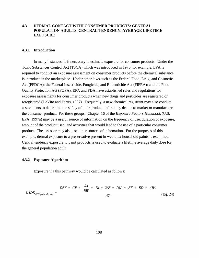
4.3 DERMAL CONTACT WITH CONSUMER PRODUCTS: GENERAL POPULATION ADULTS, CENTRAL TENDENCY, AVERAGE LIFETIME EXPOSURE
4.3.1 Introduction
In many instances, it is necessary to estimate exposure for consumer products. Under the Toxic Substances Control Act (TSCA) which was introduced in 1976, for example, EPA is required to conduct an exposure assessment on consumer products before the chemical substance is introduce in the marketplace. Under other laws such as the Federal Food, Drug, and Cosmetic Act (FFDCA); the Federal Insecticide, Fungicide, and Rodenticide Act (FIFRA); and the Food Quality Protection Act (FQPA), EPA and FDA have established rules and regulations for exposure assessments for consumer products when new drugs and pesticides are registered or reregistered (DeVito and Farris, 1997). Frequently, a new chemical registrant may also conduct assessments to determine the safety of their product before they decide to market or manufacture the consumer product. For these groups, Chapter 16 of the Exposure Factors Handbook (U.S. EPA, 1997a) may be a useful source of information on the frequency of use, duration of exposure, amount of the product used, and activities that would lead to the use of a particular consumer product. The assessor may also use other sources of information. For the purposes of this example, dermal exposure to a preservative present in wet latex household paints is examined. Central tendency exposure to paint products is used to evaluate a lifetime average daily dose for the general population adult.
4.3.2 Exposure Algorithm
Exposure via this pathway would be calculated as follows:
(Eq. 24)
108

where:
LADDABSpaint dermal
DSY
=
=
absorbed lifetime average daily dose from dermal contact with paint (mg/kg-day); density of product (g/cm3);
CF SA/BW
= =
conversion factor (mg/g); surface area of the skin that is exposed to paint (cm2/kg/event) divided by body weight;
Th = film thickness on skin (cm); WF = weight fraction of preservative in paint; DIL = dilution of product; EF = event frequency (events/year); ED = exposure duration (years); ABS = absorption fraction, this value is chemical specific; and AT = averaging time (days).
4.3.3 Exposure Factor Inputs
DSY - The density of wet latex paint is 1.24 g/cm3. This is based on the mean density of latex paint (U.S. EPA, 1986a).
CF - A conversion factor of 1,000 is needed to convert grams to milligrams for the purposes of calculating a LADD.
SA/BW - In order to predict the surface area to body weight ratio, exposed skin surface area must be measured. For this example scenario (i.e., painting), it is assumed that an individual will wear short pants and a short sleeve shirt. Thus, the exposed skin may include the hands, forearms, and lower legs. It is assumed that paint on the face and neck would be washed off immediately after application.
The age group that will be examined is all adults over 18 years of age. Table 6-9 of the Exposure Factors Handbook (U.S. EPA, 1997a) presents descriptive statistics based on the surface area/body weight ratios. The mean surface area to body weight (SA/BW) ratio is 0.0284 m2/kg (e.g., 284 cm2/kg). Table 6-5 of the Exposure Factors Handbook (U.S. EPA, 1997a) provides the percentage of total body surface areas for adults. The following table provides the
109
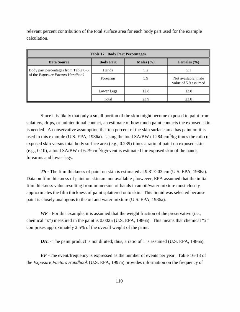
relevant percent contribution of the total surface area for each body part used for the example calculation.
Table 17. Body Part Percentages.
Data Source Body Part Males (%) Females (%)
Body part percentages from Table 6-5 of the Exposure Factors Handbook
Hands 5.2 5.1
Forearms 5.9 Not available; male value of 5.9 assumed
Lower Legs 12.8 12.8
Total 23.9 23.8
Since it is likely that only a small portion of the skin might become exposed to paint from splatters, drips, or unintentional contact, an estimate of how much paint contacts the exposed skin is needed. A conservative assumption that ten percent of the skin surface area has paint on it is used in this example (U.S. EPA, 1986a). Using the total SA/BW of 284 cm2/kg times the ratio of exposed skin versus total body surface area (e.g., 0.239) times a ratio of paint on exposed skin (e.g., 0.10), a total SA/BW of 6.79 cm2/kg/event is estimated for exposed skin of the hands, forearms and lower legs.
Th - The film thickness of paint on skin is estimated at 9.81E-03 cm (U.S. EPA, 1986a). Data on film thickness of paint on skin are not available ; however, EPA assumed that the initial film thickness value resulting from immersion of hands in an oil/water mixture most closely approximates the film thickness of paint splattered onto skin. This liquid was selected because paint is closely analogous to the oil and water mixture (U.S. EPA, 1986a).
WF - For this example, it is assumed that the weight fraction of the preservative (i.e., chemical “x”) measured in the paint is 0.0025 (U.S. EPA, 1986a). This means that chemical “x” comprises approximately 2.5% of the overall weight of the paint.
DIL - The paint product is not diluted; thus, a ratio of 1 is assumed (U.S. EPA, 1986a).
EF -The event/frequency is expressed as the number of events per year. Table 16-18 of the Exposure Factors Handbook (U.S. EPA, 1997a) provides information on the frequency of
110

occasions spent painting the interior of a home per year. The overall mean for painting with latex paints is 4 events/year (i.e., 4 days/year) (U.S. EPA, 1997a).
ED- Exposure duration is the length of time over which exposure occurs. For consumer products, exposure duration could be set equal to the length of time a product or chemical is expected to remain in the marketplace or some other measure of the length of time that a consumer will be exposed. The assumption in this example is that the exposed population may use paint containing the chemical being evaluated for 20 years, which is the time the product is assumed to be on the market.
ABS - This value is chemical specific. Information on absorption fractions can be obtained from EPA’s Dermal Exposure Assessment: Principles and Applications (U.S. EPA, 1992b). EPA has also developed the draft Part E Supplemental Guidance for Dermal Risk Assessment of the Risk Assessment Guidance for Superfund, Volume I: Human Health Evaluation Manual (U.S. EPA, 1999). This document is a source of data on dermal absorption. Although this document is not final, it is generally more representative of current thinking in this area and assessors are encouraged to use it instead of U.S. EPA (1992b). For the purposes of the calculations provided below for this example, it is assumed that the absorption fraction for the chemical of interest (i.e., chemical “x”) is 0.1.
AT - Because the lifetime average daily dose is being calculated for a member of the general population, the averaging time is equivalent to the lifetime of the individual being evaluated. For the purposes of this example, the average lifetime for men and women is used because the exposures are assumed to reflect the general population and are not gender- or age-specific. The averaging time of 70 years is used in the calculations; this value is converted to 25,550 days (i.e., 70 years * 365 days/year).
4.3.4 Calculations
Using the exposure algorithm and exposure factor inputs shown above, the LADDABS paint
dermal would be calculated as follows.
111

4.3.5 Exposure Characterization and Uncertainties
The example presented here is used to represent central tendency exposures among general population adults from dermal contact with paint. High-end exposures may be estimated by replacing the mean surface areas to body weight ratios used here with upper-percentile values. Caution should be used, however, in using upper-percentile values when average body weights are used because of the correlation between these two factors. Exposure frequencies may also be increased for estimating high-end exposures. For example, the 95th percentile exposure frequency listed in Table 16-18 of the Exposure Factors Handbook (U.S. EPA, 1997a) is 10 events per year. There are uncertainties associated with the exposed skin surface area assumed for this example (i.e., 10 percent of the hands, forearms, and lower legs). Further, hair on these body parts may limit direct deposition on the skin. Uncertainties also exist for both the film thickness and density. The film thickness is based on closely related liquids because actual film thickness data for paint were not available. These values should only be viewed as estimates and the values would be improved if actual experimental data were utilized. It appears that the uncertainty for density would be lower because density data are typically provided by manufacturers of consumer products and are based on actual experimental data. As a result of these factors, there is a moderate level of uncertainty for this assessment.
112

4.4 DERMAL CONTACT WITH SURFACE WATER: RECREATIONAL CHILDREN, CENTRAL TENDENCY, AVERAGE LIFETIME EXPOSURE
4.4.1 Introduction
The potential for exposure to chemical substances exists at sites where localized surface water bodies (i.e., streams, ponds, lakes, bays, or rivers) have been contaminated. Both adults and children may dermally absorb chemicals that are in the water as a result of activities such as swimming or wading. Receptors could include recreational swimmers or waders that trespass onto a site or commercial/industrial workers working in and around water (e.g., construction around reservoirs and drainage ditches and sampling activities to measure water quality). Exposure via dermal contact considers not only chemical concentrations in contact with the skin, but also the surface area of the skin that contacts the water, the absorption of the chemical that comes into contact with the skin, exposure duration, exposure time, and exposure frequency. For the purposes of this example, surface water exposure among recreational child swimmers and waders (age 7-12 years) is assumed. Dermal exposure is assessed based on central tendency lifetime average daily intakes.
4.4.2 Exposure Algorithm
Exposure via this pathway would be calculated as follows:
(Eq. 25)
where:
LADDABS surface water dermal = absorbed lifetime average daily dose from dermal contact with contaminated surface water (mg/kg-day);
DAevent = absorbed dose per event (mg/cm2/event); SA = surface area of the skin that contacts surface water
(cm2); EV = event frequency (events/day);
113

EF = exposure frequency (days/year); ED = exposure duration (years); BW = body weight of a child (kg); and AT = averaging time (days).
4.4.3 Exposure Factor Inputs
DAevent - The absorbed dose per event (DAevent) is estimated to consider the following factors:
C the permeability coefficient from water; C the chemical concentration in water; and, C the event duration.
The approach to estimate DAevent differs with respect to inorganic and organic chemicals. This is consistent with current EPA policy directives (U.S. EPA 2001b; U.S. EPA 1997a; U.S. EPA 1992b). Note that this is an update from previous EPA policy directives (U.S. EPA 1989). For inorganics, EPA recommends using the steady state approach to estimate dermally absorbed doses. In this approach:
DAevent = FA x Kp x Cw (Eq. 26)
where:
DAevent = Absorbed dose per event (mg/cm2/event); FA = Fraction absorbed (dimensionless); K = Dermal permeability coefficient of compound in water (cm/hr); and p
Cw = Chemical concentration in water (mg/cm3 or mg/mL).
For organics, the EPA provides two equations. These equations are different based on the event duration versus the lag time per event. If the duration of the event (tevent) is less then the time to reach steady state (2.4 x J) then the following equation is used to estimate DAevent (U.S. EPA, 2001b; U.S. EPA, 1992b):
114

where:
DA = /cm2/event); FA = Kp = Cw = /cm3 ); J = ); and, t =
J)
(U.S. EPA 1999; U.S. EPA 1992b):
(Eq. 28)
event Absorbed dose per event (mgFraction absorbed (dimensionless); Dermal permeability coefficient of compound in water (cm/hr); Chemical concentration in water (mg or mg/mLLag time per event (hr/event
event Event duration (hr/event).
If the duration of the event (tevent) is greater than the time to reach steady state (2.4 * then the equation incorporates a new coefficient B, which is a dimensionless ratio of the permeability coefficient of a compound through the stratum corneum relative to its permeability across the epidermis. The following equation is used to estimate this DAevent
(Eq. 27)
where:
DAevent = Absorbed dose per event (mg/cm2/event); FA = Fraction absorbed (dimensionless); Kp = Dermal permeability coefficient of compound in water (cm/hr); Cw = Chemical concentration in water (mg/cm3 or mg/mL); J = Lag time per event (hr/event); tevent = Event duration (hr/event); and, B = Dimensionless ratio of the permeability coefficient of a compound through
stratum corneum relative to its permeability coefficient across the viable epidermis.
115

Guidance for using these equations is detailed in Section 5.3.2- Estimating DAevent for Organics from the document entitled Dermal Exposure Assessment: Principles and Applications (U.S. EPA, 1992b). For the purposes of this example the organic chemical phenol is used. Phenol, which is identified on Table 5-7 of U.S. EPA (1992b) and Appendix A of RAGS, Part E (U.S. EPA, 2001b), has a molecular weight (MW) of 94, a log Kow of 1.46. The Kp for phenol is 4.3E-03 cm/hr and the FA is 1.0, as shown in Appendix A of EPA’s RAGS, Part E (U.S. EPA, 2001b). In order to identify which equation must be used to calculate DAevent. The lag time per event (J) must be calculated. The following equation can be used :
(Eq. 29)
In this equation lsc (the thickness of the stratum corneum) is 10-3 cm; therefore, Dsc (the stratum corneum diffusion coefficient) would be 5.1x10⁻⁷ cm2/hr.
(Eq. 30)
The lag time per event (J) is 0.36 hr. Since the time to reach steady-state (t*) is defined as 2.4 J, the t* would actually be 0.86 hr. The values for lag time per event (J), permeability ratio (B) , and steady-state (t*) can be verified on Table B-3, of RAGS Part E (U.S. EPA, 2001b). Based on Table 15-67 on page 15-83 of the Exposure Factors Handbook (U.S. EPA, 1997a), the exposure time for swimming for a child age 5-11 years is 1 hour per day, which is the 50th percentile for swimming in fresh water swimming pools. Using this value as the event duration (tevent), tevent > t*, thus Equation 28 would be used for the calculation of DAevent. The term B must be calculated:
(Eq. 31)
In the case of phenol, B=0.016. Assuming a concentration in water (Cw) of 1 mg/mL an example calculation is provided as follows:
116
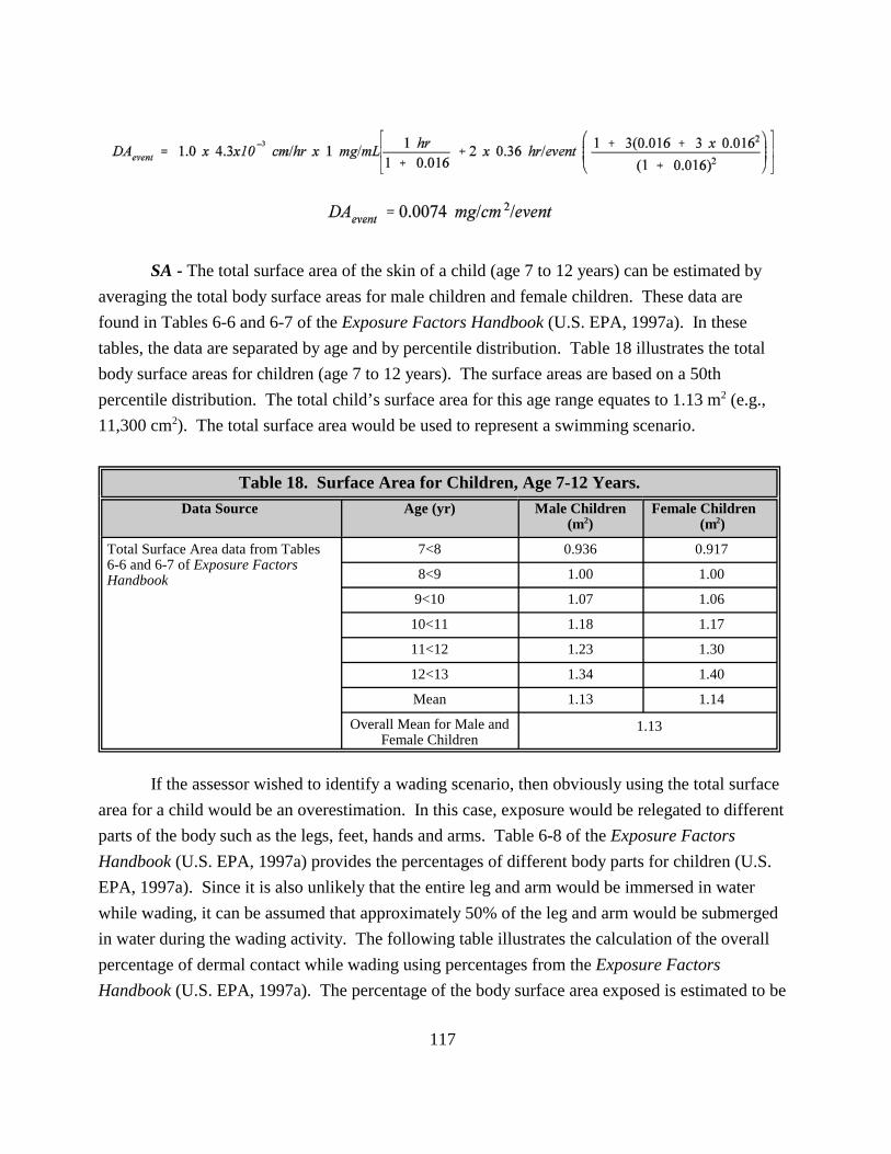
SA - The total surface area of the skin of a child (age 7 to 12 years) can be estimated by averaging the total body surface areas for male children and female children. These data are found in Tables 6-6 and 6-7 of the Exposure Factors Handbook (U.S. EPA, 1997a). In these tables, the data are separated by age and by percentile distribution. Table 18 illustrates the total body surface areas for children (age 7 to 12 years). The surface areas are based on a 50th percentile distribution. The total child’s surface area for this age range equates to 1.13 m2 (e.g., 11,300 cm2). The total surface area would be used to represent a swimming scenario.
Table 18. Surface Area for Children, Age 7-12 Years. Data Source Age (yr) Male Children
(m2) Female Children
(m2)
Total Surface Area data from Tables 6-6 and 6-7 of Exposure Factors Handbook
7<8 0.936 0.917
8<9 1.00 1.00
9<10 1.07 1.06
10<11 1.18 1.17
11<12 1.23 1.30
12<13 1.34 1.40
Mean 1.13 1.14
Overall Mean for Male and Female Children
1.13
If the assessor wished to identify a wading scenario, then obviously using the total surface area for a child would be an overestimation. In this case, exposure would be relegated to different parts of the body such as the legs, feet, hands and arms. Table 6-8 of the Exposure Factors Handbook (U.S. EPA, 1997a) provides the percentages of different body parts for children (U.S. EPA, 1997a). Since it is also unlikely that the entire leg and arm would be immersed in water while wading, it can be assumed that approximately 50% of the leg and arm would be submerged in water during the wading activity. The following table illustrates the calculation of the overall percentage of dermal contact while wading using percentages from the Exposure Factors Handbook (U.S. EPA, 1997a). The percentage of the body surface area exposed is estimated to be
117

34% based on data for ages 9<10 years and 12<13 years only (data for the other age groups considered in this example were not available). An estimate of the total child surface area used to represent a wading scenario for children (age 7 to 12 years) would be 3,842 cm2.
Table 19. Body Surface Area Exposed During Wading.
Data Source Age Arms Hands Legs Feet
Percentage of Total Body Surface Area from Table 6-8 of the
Exposure Factors Handbook
9<10 6.15 5.30 14.35 7.58
12<13 6.85 5.39 15.25 7.03
Avg 6.5 5.35 14.8 7.31
Total % 34
EV - The event frequency is the number of events per day since the LADD accounts for daily exposure. For the purposes of this example 1 event is assumed per day.
EF - Since the event/frequency is expressed as number of events per day, exposure frequency (EF) is expressed in days/yr. Table 15-176 of the Exposure Factors Handbook (U.S. EPA, 1997a) recommends using a value of one swimming event per adult per month. This is the recommended time for swimming at an outdoor swimming pool. Table 15-65 provides a more conservative estimate of the number times swimming per month based on age. Note that for the particular age group examined for this example (age 7 to 12 years), no data are available. Thus, data for the nearest age group (i.e., 5 to 11 years) may be used as surrogates. According to the table, the number of respondents for this age group (total N) is 100. Using the 50th percentile frequency for this age group, up to five events per month is estimated as the number of swimming and wading events for the summer months. It should be noted that these results are based on swimming at a pool and may not be entirely representative of wading or swimming in a lake, pond or stream. Therefore, one swimming event per month for children is assumed in this example.
Because children would typically only swim or wade during the summer months, an estimate of 5 months per year is used. Assuming one swimming/wading event per month and swimming/wading five months per year, an exposure frequency of five days per year is assumed.
118

ED - Exposure duration (ED) is the length of time over which exposure occurs. For the purposes of this example, the exposure duration for 7 to 12 year old school children is assumed to be six years. This assumes that six years are spent swimming or wading in contaminated lakes, ponds or streams near their homes.
BW - Table 7-6 of the Exposure Factors Handbook (U.S. EPA, 1997a) reports body weights for children from 6 months to 20 years old. Using the published body weights for boys and girls aged 7 to 12 years, an average weight of 32.9 kg is calculated. This is the 50th percentile of the distribution.
AT - Because the lifetime average daily dose is being calculated, the averaging time is equivalent to the lifetime of the individual being evaluated. For the purposes of this example, the average lifetime for men and women is used because the exposures are assumed to reflect the general population and are not gender- or age-specific. The averaging time of 70 years is used in the calculations. This value is converted to 25,550 days (i.e., 70 years * 365 days/year).
4.4.4 Calculations
Using the exposure algorithm and exposure factor inputs shown above, the LADDABS surface
water dermal would be as follows for both swimming and wading.
Swimming
Wading
119
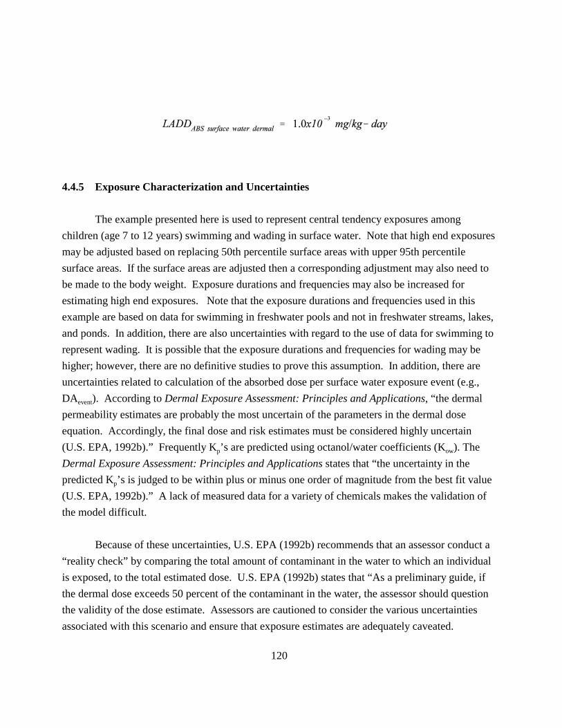
4.4.5 Exposure Characterization and Uncertainties
DA
The example presented here is used to represent central tendency exposures among children (age 7 to 12 years) swimming and wading in surface water. Note that high end exposures may be adjusted based on replacing 50th percentile surface areas with upper 95th percentile surface areas. If the surface areas are adjusted then a corresponding adjustment may also need to be made to the body weight. Exposure durations and frequencies may also be increased for estimating high end exposures. Note that the exposure durations and frequencies used in this example are based on data for swimming in freshwater pools and not in freshwater streams, lakes, and ponds. In addition, there are also uncertainties with regard to the use of data for swimming to represent wading. It is possible that the exposure durations and frequencies for wading may be higher; however, there are no definitive studies to prove this assumption. In addition, there are uncertainties related to calculation of the absorbed dose per surface water exposure event (e.g.,
event). According to Dermal Exposure Assessment: Principles and Applications, “the dermal permeability estimates are probably the most uncertain of the parameters in the dermal dose equation. Accordingly, the final dose and risk estimates must be considered highly uncertain (U.S. EPA, 1992b).” Frequently Kp’s are predicted using octanol/water coefficients (Kow). The Dermal Exposure Assessment: Principles and Applications states that “the uncertainty in the predicted Kp’s is judged to be within plus or minus one order of magnitude from the best fit value (U.S. EPA, 1992b).” A lack of measured data for a variety of chemicals makes the validation of the model difficult.
Because of these uncertainties, U.S. EPA (1992b) recommends that an assessor conduct a “reality check” by comparing the total amount of contaminant in the water to which an individual is exposed, to the total estimated dose. U.S. EPA (1992b) states that “As a preliminary guide, if the dermal dose exceeds 50 percent of the contaminant in the water, the assessor should question the validity of the dose estimate. Assessors are cautioned to consider the various uncertainties associated with this scenario and ensure that exposure estimates are adequately caveated.
120

5.0 REFERENCES
Calabrese, E.J., Stanek, E.J., Barnes, R., Burmaster, D.E., Callahan, B.G., Heath, J.S., Paustenbach, D., Abraham, J. & Gephart, L.A. (1996). Methodology to estimate the amount and particle size of soil ingested by children: implications for exposure assessment at waste sites [published erratum appears in Regul Toxicol Pharmacol 1997 Feb;25(1):87]. Regul Toxicol Pharmacol, 24: 264-8.
DeVito, S.C; Farris, C.A (1997). Premanufacture notification. Chemistry assistance for submitters. U.S. Environmental Protection Agency. Office of Pollution Prevention and Toxics. John Wiley & Sons, Inc.
Layton, D.W. (1993) Metabolically consistent breathing rates for use in dose assessments. Health Physics 64(1):23-36.
Ross Products Division. (1999). Mother’s Survey. Abbott Laboratories.
Stanek, E.J., Calabrese, E.J. & Barnes, R.M. (1999). Soil ingestion estimates for children in anaconda using trace element concentrations in different particle size fractions. Hum. Ecol. Risk Assess, 5: 547-558.
U.S. EPA. (1983-1989) Methods for assessing exposure to chemical substances. Volumes 1-13. Washington, DC: Office of Toxic Substances, Exposure Evaluation Division.
U.S. EPA. (1984) Pesticide assessment guidelines subdivision K, exposure: reentry protection. Washington, DC: Office of Pesticide Programs. EPA/540/9-48/001. Available from NTIS, Springfield, VA; PB-85-120962.
U.S. EPA. (1986a) Standard scenarios for estimating exposure to chemical substances during use of consumer products. Volumes I and II. Washington, DC: Office of Toxic Substance, Exposure Evaluation Division.
U.S. EPA. (1986b) Pesticide assessment guidelines subdivision U, applicator exposure monitoring. Washington, DC: Office of Pesticide Programs. EPA/540/9-87/127. Available from NTIS, Springfield, VA; PB-85-133286.
U.S. EPA. (1987) Selection criteria for mathematical models used in exposure assessments: surface water models. Washington, DC: Exposure Assessment Group, Office of Health and Environmental Assessment. WPA/600/8-87/042. Available from NTIS, Springfield, VA; PB-88-139928/AS.
121
U.S. EPA. (1988a) Superfund exposure assessment manual. Washington, DC: Office ofEmergency and Remedial Response. EPA/540/1-88/001. Available from NTIS, Springfield, VA;PB-89-135859.
U.S. EPA. (1988b) Selection criteria for mathematical models used in exposure assessments:groundwater models. Washington, DC: Exposure Assessment Group, Office of Health andEnvironmental Assessment. EPA/600/8-88/075. Available from NTIS, Springfield, VA; PB-88-248752/AS.
U.S. EPA. (1989) Risk assessment guidance for Superfund. Human health evaluation manual:Part A. Interim Final. Washington, DC: Office of Solid Waste and Emergency Response. <http://www.epa.gov/superfund/programs/risk/ragsa/index.htm>Available from NTIS, Springfield, VA; PB-90-155581.
U.S. EPA. (1990) Methodology for assessing health risks associated with indirect exposure tocombustor emissions. EPA 600/6-90/003. Available from NTIS, Springfield, VA; PB-90-187055/AS.
U.S. EPA. (1991) Risk assessment guidance for Superfund. Human health evaluation manual:Part B. Interim Final. Washington, DC: Office of Solid Waste and Emergency Response. <http://www.epa.gov/superfund/programs/risk/ragsb/index.htm>
U.S. EPA. (1991) Risk assessment guidance for Superfund. Human health evaluation manual:Part C. Interim Final. Washington, DC: Office of Solid Waste and Emergency Response. <http://www.epa.gov/superfund/programs/risk/ragsc/index.htm>
U.S. EPA (1992a) Guidelines for exposure assessment. Washington, DC: EnvironmentalProtection Agency. Federal Register Notice. Vol. 57 No. 104, pp. 22888-22938.
U.S. EPA. (1992b) Dermal exposure assessment: principles and applications. Washington, DC:Office of Health and Environmental Assessments. EPA/600/8-9/011F.
U.S. EPA. (1994) Estimating exposures to dioxin-like compounds. (Draft Report). Washington,DC: Office of Research and Development. EPA/600/6-88/005Cb.
U.S. EPA. (1996a) Summary report for the workshop on the monte carlo analysis. U.S.Environmental Protection Agency, Risk Assessment Forum, Washington, DC, EPA/630/R-96/010. 01 Sep 1996. http://cfpub.epa.gov/ncea/cfm/recordisplay.cfm?deid=30017
U.S. EPA (1996b, 2001) Soil screening guidance: Technical background document. WashingtonDC; Environmental Protection Agency, Office of Emergency and Remedial Response. EPA540/R-96/018
122

U.S. EPA (1997a) Exposure factors handbook. Washington, DC: Environmental Protection Agency, Office of Research and Development. EPA/600/P-95/002Fa,b,c.
U.S. EPA. (1997b) Guiding principles for monte carlo analysis. U.S. EPA, Risk Assessment Forum, Washington, DC, EPA/630/R-97/001. 01 Mar 1997. http://www.epa.gov/ncea/raf/montecar.pdf
U.S. EPA. (1997c) Policy for Use of Probabilistic Analysis in Risk Assessment, U.S. EPA May 15, 1997
U.S. EPA (1997d) Standard Operating Procedures (SOPs) for Residential Exposure Assessments, draft
U.S. EPA. (1998a) Guidance for submission of probabilistic exposure assessments to the office of pesticide programs’health effects division -Draft, Office of Pesticide Programs, Washington, DC http://www.epa.gov/oscpmont/sap/1998/march/backgrd.pdf
U.S. EPA. (1998b) Risk assessment guidance for Superfund. Human health evaluation manual: Part D. Interim Final. Washington, DC: Office of Solid Waste and Emergency Response. <http://www.epa.gov/superfund/programs/risk/ragsd/index.htm>
U.S. EPA. (1999) Report of the workshop on selecting input distributions for probabilistic assessments. U.S. EPA, Risk Assessment Forum, Washington, DC,630/R-98/004. 01 Jan 1999. 260 pp.http://cfpub.epa.gov/ncea/cfm/recordisplay.cfm?deid=12487
U.S. EPA. (2000a) Options for development of parametric probability distributions for exposure factors. U.S. Environmental Protection Agency, Office of Research and Development, National Center for Environmental Assessment, Washington Office, Washington, DC, EPA/600/R-00/058. 01 Jul 2000. http://cfpub.epa.gov/ncea/cfm/recordisplay.cfm?deid=20867
U.S. EPA (2000b) Revised Methodology for Deriving Health-Based Ambient Water Quality Criteria, Office of Water. EPA 822-F-00-005.
U.S. EPA. (2000c) Technical Review Workgroup for Lead. TRW Recommendations for Sampling Soil at Lead (Pb) Sites, Vol. 2000. U.S. EPA Technical Review Workgroup for Lead.
U.S. EPA. (2001a) Risk assessment guidance for superfund: Volume III - Part A, Process for conducting probabilistic assessment, Office Office of Solid Waste and Emergency Response, Washington, DC. http://www.epa.gov/superfund/programs/risk/rags3a/index.htm
U.S. EPA. ( 2001b) Risk assessment guidance for Superfund, Volume I: Human health evaluation manual (Part E, supplemental guidance for dermal risk assessment). Interim Guidance. Office of
123
Solid Waste and Emergency Response.Washington, DC. <http://www.epa.gov/superfund/programs/risk/ragse>
U.S. EPA. (2002) A Review of the reference dose and reference concentration processes. Washington, DC: Environmental Protection Agency, Risk Assessment Forum. EPA/630/P-02/002F. Available on line at http://www.epa.gov/iris/RFD_FINAL%5B1%5D.pdf
U.S. EPA. (2003) Framework for cumulative risk assessments. National Center for Environmental Assessment, Office of Research and Development. EPA/630/P-02/001F.
124