EXAMPACK - Unisa Study Notesgimmenotes.co.za/.../12/mac3701-exampack-2015-edition.pdfSTUDY NOTES..... 3 STANDARD COSTING AND VARIANCE ANALYSIS..... 15 Cost Volume Profit Analysis

Mac3701/ep/gd

EXAMPACK

MAC3701

LUCIANO SCHOOL OF LAW & SOCIAL SCIENCES [LSLSS]

March 1, 2015

Authored by: Naphtali

1


Contents

STUDY NOTES ................................................................................................................................................ 3

BUDGETING: ............................................................................................................................................ 13

STANDARD COSTING AND VARIANCE ANALYSIS ..................................................................................... 15

Cost Volume Profit Analysis ....................................................................................................................... 18

CVP Analysis Formula ............................................................................................................................. 18

Contribution Margin (CM) .................................................................................................................. 18

Unit Contribution Margin (Unit CM) .................................................................................................. 18

Contribution Margin Ratio (CM Ratio) .............................................................................................. 19

Contribution margin and contribution margin ratio ............................................................................. 19

Break-even point .................................................................................................................................... 20

Targeted income ..................................................................................................................................... 23

DEFINITION of 'Sensitivity Analysis' ........................................................................................................ 33

The Benefits of What-if Analysis ............................................................................................................ 34

Common What-if Analysis Methods ...................................................................................................... 34

Example .................................................................................................................................................. 35

PROCESS COSTING .................................................................................................................................. 37

Joint products ..................................................................................................................................... 37

By-products......................................................................................................................................... 37

Treatment of joint costs ......................................................................................................................... 38

Accounting treatment for joint products .......................................................................................... 38

Accounting treatment for by-products .............................................................................................. 38

Relevant Costing ......................................................................................................................................... 42

Example .................................................................................................................................................. 42

DEFINITION of 'Relevant Cost' ............................................................................................................... 43

INVESTOPEDIA EXPLAINS 'Relevant Cost'.............................................................................................. 43

Concept ................................................................................................................................................... 47

Types of Relevant Costs ......................................................................................................................... 48

Types of Non-Relevant Costs ................................................................................................................. 48

Example .................................................................................................................................................. 48

Relevant Cost .......................................................................................................................................... 49

http://www.lslss.co.za/


2


Manufacturing Cost ................................................................................................................................ 50

Application & Limitations ...................................................................................................................... 51

QUALITATIVE DECISION MAKING: .......................................................................................................... 55

FEEDBACK FROM PAST PAPERS .............................................................................................................. 58

MAY/JUNE 2014 .................................................................................................................................. 58

ADDITIONAL QUESTIONS ........................................................................................................................ 70

Set one ................................................................................................................................................ 70

Answers to Set One Questions............................................................................................................ 78



3


STUDY NOTES STUDY UNIT 1-Advanced Behavioural aspects of Costs

In second year cost and management accounting, you studied on the classification of costs and the behaviour of costs. Three nature of costs can be determined in manufacturing, i. e, variable, fixed and semi-variable. This study unit goes further into the determination of the.

1. Behaviour of Variable costs of Inventory using the most widely used inventory control 2. Behaviour of semi-variable costs using the simple correlation and regression analysis.

Note that, importance of the knowledge of the High-low method cannot be over emphasised since it is the one of the most important aspects in management accounting

3. Behaviour of variable costs of labour using the learning curve concept. We shall first focus on the splitting and behaviour of the semi-variable costs using the simple correlation and regression analysis. Simple correlation and regression analysis. Variable costs are one of the key costs in manufacturing. It is however of great importance to split these costs into their variable costs element (b) and their fixed costs component (a). Before this can be done, it is vital to know the variable which influences the behaviour of these semi-variable costs. In each question, two or more variables will be given, however when more than two variables are given only two are of importance. One of the important variables, causes the other’s behaviour and this is an independent variable (x), while the other variable’s behaviour is determined by the independent variable, we call this the dependent variable (y). The relationship between (x) and (y) and be measured by the correlation coefficient (r). When +0, 75< r < +1 or -0, 75< r <-1 there is a relationship between the two variables and hence the regression or least squares method is useful. This relationship can be positive or negative. The High-low method can only be used when there is a perfect relationship between x and y, or anything close to perfect. Q1. Michal Ltd manufactures a single product. In addition to other costs are manufacturing overheads of the previous ten months. Month Production Overheads (Units) (R) 1 1500 800 2 2000 1000 3 3000 1350 4 2500 1250



4


5 3000 1300 6 2500 1200 7 3500 1400 8 3000 1250 9 2500 1150 10 1500 800 Other costs incurred include Material @ R9.75 per 100 units, Labour @ 9.00 per 100 units and fixed costs of R631.25 per month. It also anticipated that month 11 will have a capacity of 4000 units and all costs are paid for in cash. REQUIRED

(a) Is there a relationship between production quantity and manufacturing overheads (5) (b) Use the least-squares method to determine the variable cost element and fixed costs

component of manufacturing overheads (5) (c) Can the High-low method be used in this case, if so use it to determine the fixed cost

component and the variable cost element, more so, give reasons why it can or cannot be used (5)

(d) Calculate the cash requirement for month 11, from the available particulars (4)



5


Learning Curve This concept is used in relation to the direct labour cost or wages in production, when the time rate system is in use. The principle of specialisation is applied only up to a specific unit manufactured (32 units) whereby a certain rate (learning rate) is applied with every unit of doubling. Whenever units double the rate of learning applies thus, 1-2-4-8-16-32. This learning rate can be expressed as a percentage and then its name becomes learning curve. Therefore we are saying, as a worker continues to manufacture the same product, s/he becomes better and better in terms of time use rippling to the cost of labour since the time rate system of payment will be in use. Q2. Naphtali Ltd designs and manufactures exclusive dresses. An order of 16 identical dresses of an original design was received. The dresses are sold by ‘Boutique 4 U’ a chain of boutiques situated in all major cities in the country. The direct labour costs at R6 per hour, to manufacture the first two dresses is as follows. First dress R150. Both dresses R270. An increase in the wage rate was agreed upon, and is applicable to the remaining number of dresses at 10% increment. The designer earns R5760 per month and designs approximately 18 new creations in each month. Each dress requires 4.5 metres of material which has a factory cost of R17 per metre. It was estimated that sundry items, like decorative trimmings, buttons and cotton, will amount to R7 per dress. The following basis was determined to allocate the replacement and maintenance costs of machines used: -sewing machines at R0.50 per direct labour hour -over lockers at R0.75 per direct labour hour Monthly fixed costs of the company amount to R7, 550. Of which this order should bear 2%. The rate of learning is expected to remain constant up to the completion of the order and each dress is expected to be sold for R26.25.



6


REQUIRED What is the expected net income from this order (15) Round all rand values off to the nearest rand.



7


INVENTORY CONTROL AND THE USE OF THE ECONOMIC ORDER QUANTITY. Inventory is one of the greatest costs for manufacturing and engineering enterprises, therefore strict control is important for efficient and effective operations as well as the reduction of costs and optimisation of the resources available. Traditionally, entities bought inventories in bulk and kept them in the warehouses. The Japanese however introduced more efficient inventory control systems of the Just-In-Time (JIT), and the Economic Order Quantity (EOQ). The JIT is when inventories are acquired just before production of a placed order so as to reduce storage or holding costs. However the JIT system requires very reliable and efficient suppliers which is highly unlikely. Meanwhile two of the major inventory costs are holding costs and ordering costs. The EOQ therefore tries to optimise these costs by attempting to get the least cost identified for both types of inventory cost. The EOQ has become a widely used control system for inventory management.



8


Q3. Hooked-on-music Ltd is a wholesaler of portable compact disk cd-players. The company sells approximately 1500 cd-players per month. Sales take place evenly throughout the year, which consists of 300 working days. The company currently purchases the cd-players at a cost of R350 each. Orders are executed within 5 days. Safety stock should amount to the sales requirement for 3 working days. There is no seasonal fluctuation in the demand for cd-players. According to estimate, the cost to place an order amounts to R150. The enterprise requires a pre-tax return on capital of 20%. In addition to the required rate of return, direct stockholding costs, excluding insurance at 7% of the unit cost per year, amount to R10.50 per unit. The company has been approached by another supplier, offering a price of R330 per cd-player, provided that orders are placed in batches of at least 450 units each. The lead time for delivery would remain 5 days. The ordering cost per order will remain the same. The current rates of inflation and tax are 8% and 30% respectively. REQUIRED

(a) Determine the number of orders to be placed annually, without taking the special offer into account. (8)

(b) Determine the re-order point for cd-players (3) (c) Determine whether the special offer should be accepted, or not. (Show your detailed

calculations.) (15)



9


Activity-based costing (ABC) is a costing methodology that identifies activities in an organization and assigns the cost of each activity with resources to all products and services according to the actual consumption by each. This model assigns more indirect costs (overhead) into direct costs compared to conventional costing.

CIMA (Chartered Institute of Management Accountants) defines ABC as an approach to the costing and monitoring of activities which involves tracing resource consumption and costing final outputs. Resources are assigned to activities, and activities to cost objects based on consumption estimates. The latter utilize cost drivers to attach activity costs to outputs.

Activity based costing (ABC) assigns manufacturing overhead costs to products in a more logical manner than the traditional approach of simply allocating costs on the basis of machine hours. Activity based costing first assigns costs to the activities that are the real cause of the overhead. It then assigns the cost of those activities only to the products that are actually demanding the activities.

Activity-based costing (ABC) is a better, more accurate way of allocating overhead.

Recall the steps to product costing:

1. Identify the cost object; 2. Identify the direct costs associated with the cost object; 3. Identify overhead costs; 4. Select the cost allocation base for assigning overhead costs to the cost object; 5. Develop the overhead rate per unit for allocating overhead to the cost object.

Activity-based costing refines steps #3 and #4 by dividing large heterogeneous cost pools into multiple smaller, homogeneous cost pools. ABC then attempts to select, as the cost allocation base for each overhead cost pool, a cost driver that best captures the cause and effect relationship between the cost object and the incurrence of overhead costs. Often, the best cost driver is a nonfinancial variable.



http://en.wikipedia.org/wiki/Indirect_costs

http://en.wikipedia.org/wiki/Overhead_%28business%29

http://en.wikipedia.org/wiki/Direct_costs

10


ABC can become quite elaborate. For example, it is often beneficial to employ a two-stage allocation process whereby overhead costs are allocated to intermediate cost pools in the first stage, and then allocated from these intermediate cost pools to products in the second stage. Why is this intermediate step useful? Because it allows the introduction of multiple cost drivers for a single overhead cost item. This two-stage allocation process is illustrated in the example of the apparel factory below.

ABC focuses on activities. A key assumption in activity-based costing is that overhead costs are caused by a variety of activities, and that different products utilize these activities in a non-homogeneous fashion. Usually, costing the activity is an intermediate step in the allocation of overhead costs to products, in order to obtain more accurate product cost information. Sometimes, however, the activity itself is the cost object of interest. For example, managers at Levi Strauss & Co. might want to know how much the company spends to acquire denim fabric, as input in a sourcing decision. The “activity” of acquiring fabric incurs costs associated with negotiating prices with suppliers, issuing purchase orders, receiving fabric, inspecting fabric, and processing payments and returns.



11


Just in time (JIT) is a production strategy that strives to improve a business' return on investment by reducing in-process inventory and associated carrying costs. Just in time is a type of operations management approach which originated in Japan in the 1950s. It was adopted by Toyota and other Japanese manufacturing firms, with excellent results: Toyota and other companies that adopted the approach ended up raising productivity (through the elimination of

waste) significantly. To meet JIT objectives, the process relies on signals or Kanban (看板?, Kanban) between different points, which are involved in the process, which tell production when to make the next part. Kanban are usually 'tickets' but can be simple visual signals, such as the presence or absence of a part on a shelf. Implemented correctly, JIT focuses on continuous improvement and can improve a manufacturing organization's return on investment, quality, and efficiency. To achieve continuous improvement key areas of focus could be flow, employee involvement and quality.

JIT relies on other elements in the inventory chain as well. For instance, its effective application cannot be independent of other key components of a lean manufacturing system or it can "end up with the opposite of the desired result. “In recent years manufacturers have continued to try to hone forecasting methods such as applying a trailing 13-week average as a better predictor for JIT planning; however, some research demonstrates that basing JIT on the presumption of stability is inherently flawed.

A good example would be a car manufacturer that operates with very low inventory levels, relying on their supply chain to deliver the parts they need to build cars. The parts needed to manufacture the cars do not arrive before nor after they are needed, rather they arrive just as they are needed. This inventory supply system represents a shift away from the older "just in case" strategy where producers carried large inventories in case higher demand had to be met.



http://en.wikipedia.org/wiki/Return_on_investment


http://en.wikipedia.org/wiki/Inventory

http://en.wikipedia.org/wiki/Carrying_cost

http://en.wikipedia.org/wiki/Kanban

http://en.wikipedia.org/wiki/Help:Installing_Japanese_character_sets



http://en.wikipedia.org/wiki/Lean_manufacturing

12




13


BUDGETING:

A budget is a forecasted statement expressed in monetary or quantitative statement (a

financial plan of action for the future). The key purpose of a budget is to determine the most

profitable financial strategy for the Company. Budgeting is therefore the process of developing

budgets within an entity, modern studies propose budgets to be done by a budgeting team

through a process known as effective budgeting ( THE INVOLVEMENT OF EMPLOYEES AND

JUNIORS IN THE BUDGETORY PROCESS). Most entities however ignore this concept of

budgeting which is at the heart of business achievement. The budgeting team is led by a budget

manager usually an accountant or finance person.

Budgets can be Capital Budgets or Operational Budgets. Our focus shall be on the operational

budgets.

Advantages of budgeting.

Enhances good communication within an entity

It paves direction for the team and the company as a whole

If done properly, it sets a tone or pace for good management

Enhances co-ordination

Guides personnel to understand expectations and how they will be evaluated

Isolate problem areas and enable corrective action to be taken before problems arise (it

is pro-active than reactive)

Highlight the importance of cost considerations in company operations

Ensures all levels of management co-operate towards a common goal

Causes all sections to co-ordinate their activities and define specific areas of

responsibility

Helps corporate policies and organisational structures to be defined.

Types of operational budgets

The master budget- consists of a list of the goods and services the company plans to

consume during the operating period and the benefits it expects its activities to

produce. As a whole, it contains all departmental operating schedules, budgets and

ultimately the budgeted financial statements.

The master budget consists of the following sub-budgets.

1. Capital budget- focuses its attention on long-term investment decisions and the

financing of those investments.

2. Operational budget



14


-the emphases of operational budgeting is entirely on business profitability and the

compilation of the financial statements. The sub-components of these operational

budgets include quantity and monetary budgets like

- Sales budget

- Production budget

- Material Usage budget

- Material purchase budget

- Cost of Sales budget

- Labour budget

- Overhead budget

- Cash budget

- Income Statement

- Balance Sheet

Approach to budgeting

- Top-down

- Bottom-up

Zero-Based Budgeting approach

A zero-based budget is really a budget that starts from a zero factor. It disregards all previous

results like the traditional methods of extrapolating figures. This approach is entirely based on

the principal factor of zero until the manager in-charge proves otherwise the factor remains at

zero. Its major negative implication or drawback is on routine managers who are comfortable

with the cosy status quo.

Qn. Discuss the implications of ZBB (15).

Qn. Discuss the implications of Budgeting (15).



15


STANDARD COSTING AND VARIANCE ANALYSIS

A standard cost is a targeted or expected cost.

Types of Standard. There are three types of standards namely.

Basic standards- those which remain unchanged regardless of the circumstance e. g

distance

Ideal standards-those based on maximum and efficient production, which do not

consider slack, idle time, change-overs e. t. c. they are basically unattainable in nature.

Attainable standards-also based on maximum production but they do take slack and

other circumstances into consideration. These standards form the foundation of our

study.

Standard costing develops from the need to compare the budget with the actual production.

Variance analysis.

This is the comparison of budget/standard with actual results. The difference yields a variance

and these variances are described as either favourable (+ve) or unfavourable/adverse (-ve). The

analysis of variances go further into determining the reasons for the variance.

Types of variances. (BASIC)

Sales variances

Material variances

Labour variances

Further variances.

Mix variances

Yield variances

Idle time

Fixed overhead variances

Variable overhead variances

Fixed admin variances

Variable admin variances

Fixed selling variances

Variable selling variances

Qn. what are the advantages and disadvantages of standard costing and variance analysis (15).

Qn. what are the uses and in what environments can standard costing be used (20).



16


Divisional Performance Measures

Large companies normally have divisions which perform different activities or produce different

products. Due to the complexity of the operations it’s a challenge for top management to have

control of all operations. Various managers are set to oversee the operations for specific

divisions. It is therefore of great importance for management to have uniform measures of how

the divisions are measured.

What to note:

Divisional structures

Distinction between

Advantages and disadvantages of divisionalisation

Measures- RETURN ON INVESTMENT, RESIDUAL INCOME AND ECONOMIC VALUE

ADDED (EVA) ™.

PRICING DECISIONS AND PROFITABILITY ANALYSIS.

Pricing is one of the key decisions entities have to consider carefully. Accounting information is

normally a product of pricing. It therefore very necessary for an entity to study the industry and

decide the nature of the pricing policy they adopt.

What to note:

The role of cost information in pricing

Short-run price setting

Long-run price setting

Types of pricing policies.

Competitor based pricing e. g skimming or penetration

Customer based- differential pricing, price discrimination

Cost based pricing- crocodile, break-even, mark-up, negotiation, marginal/variable,

prime cost, full cost (without mark-up), marginal plus opportunity cost.

Product life cycle pricing.

DIVISIONAL TRANSFER PRICING.

What to understand:



17


Purpose for transfer pricing

Methods for transfer pricing- market-based, cost plus mark-up, marginal/variable

cost, full cost (without mark-up), negotiation, marginal plus opportunity cost, dual

rate transfer pricing.

Recommendations for transfer pricing- local and international markets.



18


Cost Volume Profit Analysis

Cost-Volume-Profit (CVP) analysis is a managerial accounting technique that is concerned with the effect of sales volume and product costs on operating profit of a business. It deals with how operating profit is affected by changes in variable costs, fixed costs, selling price per unit and the sales mix of two or more different products.

CVP analysis has following assumptions:

1. All cost can be categorized as variable or fixed. 2. Sales price per unit, variable cost per unit and total fixed cost are constant. 3. All units produced are sold.

Where the problem involves mixed costs, they must be split into their fixed and variable component by High-Low Method, Scatter Plot Method or Regression Method.

CVP Analysis Formula

The basic formula used in CVP Analysis is derived from profit equation:

px = vx + FC + Profit

In the above formula, p is price per unit; v is variable cost per unit; x are total number of units produced and sold; and FC is total fixed cost

Besides the above formula, CVP analysis also makes use of following concepts:

Contribution Margin (CM)

Contribution Margin (CM) is equal to the difference between total sales (S) and total variable cost or, in other words, it is the amount by which sales exceed total variable costs (VC). In order to make profit the contribution margin of a business must exceed its total fixed costs. In short:

CM = S − VC

Unit Contribution Margin (Unit CM)

Contribution Margin can also be calculated per unit which is called Unit Contribution Margin. It is the excess of sales price per unit (p) over variable cost per unit (v). Thus:



19


Unit CM = p − v

Contribution Margin Ratio (CM Ratio)

Contribution Margin Ratio is calculated by dividing contribution margin by total sales or unit CM by price per unit.

Cost-volume-profit (CVP) analysis is used to determine how changes in costs and volume affect a company's operating income and net income. In performing this analysis, there are several assumptions made, including:

Sales price per unit is constant. Variable costs per unit are constant. Total fixed costs are constant. Everything produced is sold. Costs are only affected because activity changes. If a company sells more than one product, they are sold in the same mix. CVP analysis requires that all the company's costs, including manufacturing, selling, and

administrative costs, be identified as variable or fixed.

Contribution margin and contribution margin ratio

Key calculations when using CVP analysis are the contribution margin and the contribution margin ratio. The contribution margin represents the amount of income or profit the company made before deducting its fixed costs. Said another way, it is the amount of sales dollars available to cover (or contribute to) fixed costs. When calculated as a ratio, it is the percent of sales dollars available to cover fixed costs. Once fixed costs are covered, the next dollar of sales results in the company having income.

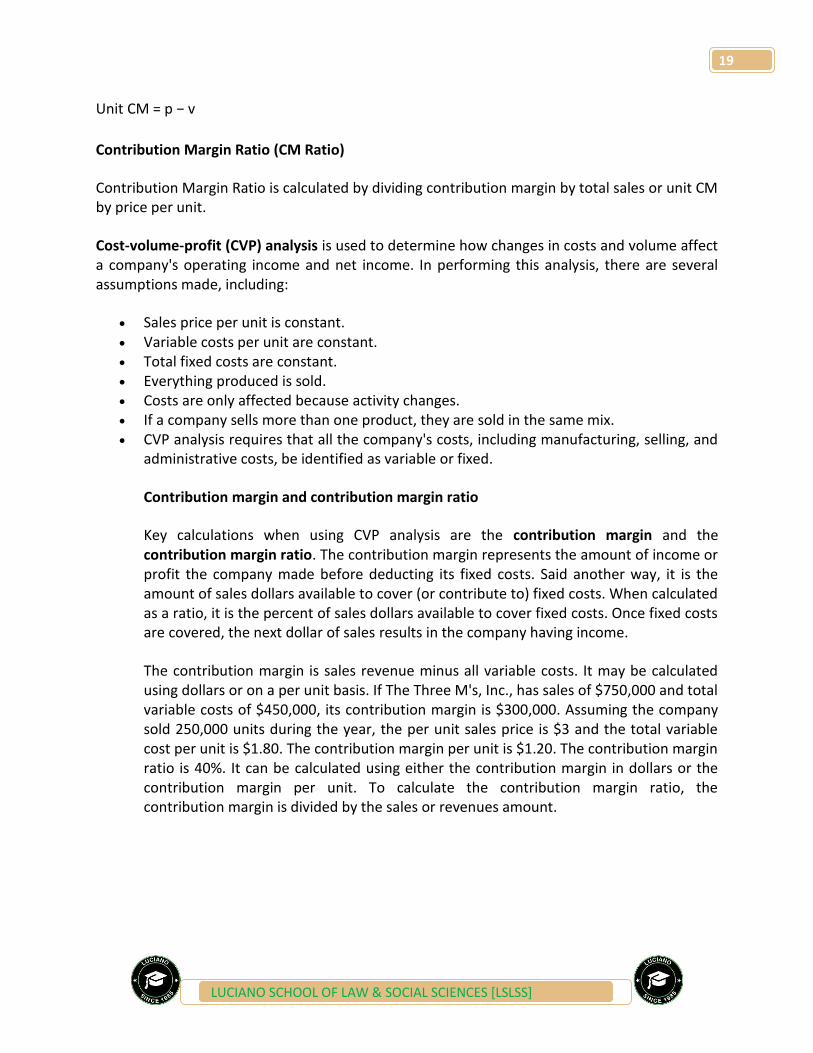
The contribution margin is sales revenue minus all variable costs. It may be calculated using dollars or on a per unit basis. If The Three M's, Inc., has sales of $750,000 and total variable costs of $450,000, its contribution margin is $300,000. Assuming the company sold 250,000 units during the year, the per unit sales price is $3 and the total variable cost per unit is $1.80. The contribution margin per unit is $1.20. The contribution margin ratio is 40%. It can be calculated using either the contribution margin in dollars or the contribution margin per unit. To calculate the contribution margin ratio, the contribution margin is divided by the sales or revenues amount.



20


Break-even point

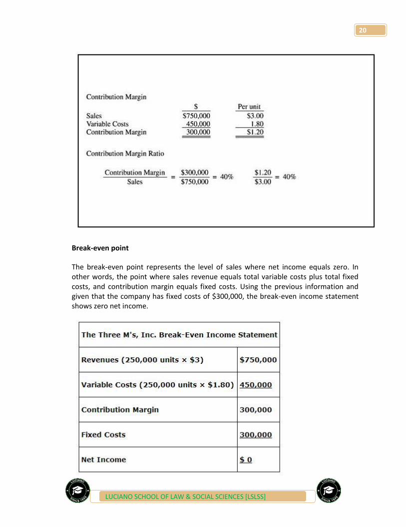
The break‐even point represents the level of sales where net income equals zero. In other words, the point where sales revenue equals total variable costs plus total fixed costs, and contribution margin equals fixed costs. Using the previous information and given that the company has fixed costs of $300,000, the break‐even income statement shows zero net income.



21


This income statement format is known as the contribution margin income statement and is used for internal reporting only.

The $1.80 per unit or $450,000 of variable costs represent all variable costs including costs classified as manufacturing costs, selling expenses, and administrative expenses. Similarly, the fixed costs represent total manufacturing, selling, and administrative fixed costs.

Break‐even point in dollars. The break‐even point in sales dollars of $750,000 is calculated by dividing total fixed costs of $300,000 by the contribution margin ratio of 40%.

Another way to calculate break‐even sales dollars is to use the mathematical equation.

In this equation, the variable costs are stated as a percent of sales. If a unit has a $3.00 selling price and variable costs of $1.80, variable costs as a percent of sales is 60% ($1.80 ÷ $3.00). Using fixed costs of $300,000, the break‐even equation is shown below.



22


The last calculation using the mathematical equation is the same as the break‐even sales formula using the fixed costs and the contribution margin ratio previously discussed in this chapter.

Break‐even point in units. The break‐even point in units of 250,000 is calculated by dividing fixed costs of $300,000 by contribution margin per unit of $1.20.

The break‐even point in units may also be calculated using the mathematical equation where “X” equals break‐even units.



23


Again it should be noted that the last portion of the calculation using the mathematical equation is the same as the first calculation of break‐even units that used the contribution margin per unit. Once the break‐even point in units has been calculated, the break‐even point in sales dollars may be calculated by multiplying the number of break‐even units by the selling price per unit. This also works in reverse. If the break‐even point in sales dollars is known, it can be divided by the selling price per unit to determine the break‐even point in units.

Targeted income



24


CVP analysis is also used when a company is trying to determine what level of sales is necessary to reach a specific level of income, also called targeted income. To calculate the required sales level, the targeted income is added to fixed costs, and the total is divided by the contribution margin ratio to determine required sales dollars, or the total is divided by contribution margin per unit to determine the required sales level in units.

Using the data from the previous example, what level of sales would be required if the company wanted $60,000 of income? The $60,000 of income required is called the targeted income. The required sales level is $900,000 and the required number of units is 300,000. Why is the answer $900,000 instead of $810,000 ($750,000 [break‐even sales] plus $60,000)? Remember that there are additional variable costs incurred every time an additional unit is sold, and these costs reduce the extra revenues when calculating income.



25


This calculation of targeted income assumes it is being calculated for a division as it ignores income taxes. If a targeted net income (income after taxes) is being calculated, then income taxes would also be added to fixed costs along with targeted net income.

Assuming the company has a 40% income tax rate, its break‐even point in sales is $1,000,000 and break‐even point in units is 333,333. The amount of income taxes used in the calculation is $40,000 ([$60,000 net income ÷ (1 – .40 tax rate)] – $60,000).

A summarized contribution margin income statement can be used to prove these calculations.



26


Cost-volume-profit analysis looks primarily at the effects of differing levels of activity on the financial results of a business

In any business, or, indeed, in life in general, hindsight is a beautiful thing. If only we could look into a crystal ball and find out exactly how many customers were going to buy our product, we would be able to make perfect business decisions and maximise profits.

Take a restaurant, for example. If the owners knew exactly how many customers would come in each evening and the number and type of meals that they would order, they could ensure that staffing levels were exactly accurate and no waste occurred in the kitchen. The reality is, of course, that decisions such as staffing and food purchases have to be made on the basis of estimates, with these estimates being based on past experience.

While management accounting information can’t really help much with the crystal ball, it can be of use in providing the answers to questions about the consequences of different courses of action. One of the most important decisions that needs to be made before any business even starts is ‘how much do we need to sell in order to break-even?’ By ‘break-even’ we mean simply covering all our costs without making a profit.

This type of analysis is known as ‘cost-volume-profit analysis’ (CVP analysis) and the purpose of this article is to cover some of the straight forward calculations and graphs required for this



27


part of the Paper F5 syllabus, while also considering the assumptions which underlie any such analysis.

THE OBJECTIVE OF CVP ANALYSIS

CVP analysis looks primarily at the effects of differing levels of activity on the financial results of a business. The reason for the particular focus on sales volume is because, in the short-run, sales price, and the cost of materials and labour, are usually known with a degree of accuracy. Sales volume, however, is not usually so predictable and therefore, in the short-run, profitability often hinges upon it. For example, Company A may know that the sales price for product x in a particular year is going to be in the region of $50 and its variable costs are approximately $30.

It can, therefore, say with some degree of certainty that the contribution per unit (sales price less variable costs) is $20. Company A may also have fixed costs of $200,000 per annum, which again, are fairly easy to predict. However, when we ask the question: ‘Will the company make a profit in that year?’, the answer is ‘We don’t know’. We don’t know because we don’t know the sales volume for the year. However, we can work out how many sales the business needs to make in order to make a profit and this is where CVP analysis begins.

Methods for calculating the break-even point The break-even point is when total revenues and total costs are equal, that is, there is no profit but also no loss made. There are three methods for ascertaining this break-even point:

1 The equation method A little bit of simple maths can help us answer numerous different cost-volume-profit questions.

We know that total revenues are found by multiplying unit selling price (USP) by quantity sold (Q). Also, total costs are made up firstly of total fixed costs (FC) and secondly by variable costs (VC). Total variable costs are found by multiplying unit variable cost (UVC) by total quantity (Q). Any excess of total revenue over total costs will give rise to profit (P). By putting this information into a simple equation, we come up with a method of answering CVP type questions. This is done below continuing with the example of Company A above.

Total revenue – total variable costs – total fixed costs = Profit (USP x Q) – (UVC x Q) – FC = P (50Q) – (30Q) – 200,000 = P

Note: total fixed costs are used rather than unit fixed costs since unit fixed costs will vary depending on the level of output.



28


It would, therefore, be inappropriate to use a unit fixed cost since this would vary depending on output. Sales price and variable costs, on the other hand, are assumed to remain constant for all levels of output in the short-run, and, therefore, unit costs are appropriate.

Continuing with our equation, we now set P to zero in order to find out how many items we need to sell in order to make no profit, ie to break even:

(50Q) – (30Q) – 200,000 = 0 20Q – 200,000 = 0 20Q = 200,000 Q = 10,000 units.

The equation has given us our answer. If Company A sells less than 10,000 units, it will make a loss; if it sells exactly 10,000 units, it will break-even, and if it sells more than 10,000 units, it will make a profit.

2 The contribution margin method This second approach uses a little bit of algebra to rewrite our equation above, concentrating on the use of the ‘contribution margin’. The contribution margin is equal to total revenue less total variable costs. Alternatively, the unit contribution margin (UCM) is the unit selling price (USP) less the unit variable cost (UVC). Hence, the formula from our mathematical method above is manipulated in the following way:

(USP x Q) – (UVC x Q) – FC = P (USP – UVC) x Q = FC + P UCM x Q = FC + P Q = FC + P UCM

So, if P=0 (because we want to find the break-even point), then we would simply take our fixed costs and divide them by our unit contribution margin. We often see the unit contribution margin referred to as the ‘contribution per unit’. Applying this approach to Company A again:

UCM = 20, FC = 200,000 and P = 0. Q = FC UCM Q = 200,000 20

Therefore Q = 10,000 units

The contribution margin method uses a little bit of algebra to rewrite our equation above, concentrating on the use of the ‘contribution margin’.



29


3 The graphical method With the graphical method, the total costs and total revenue lines are plotted on a graph; $ is shown on the y axis and units are shown on the x axis. The point where the total cost and revenue lines intersect is the break-even point. The amount of profit or loss at different output levels is represented by the distance between the total cost and total revenue lines. The gap between the fixed costs and the total costs line represents variable costs.

Alternatively, a contribution graph could be drawn. While this is not specifically covered by the Paper F5 syllabus, it is still useful to see it. This is very similar to a break-even chart, the only difference being that instead of showing a fixed cost line, a variable cost line is shown instead.

Hence, it is the difference between the variable cost line and the total cost line that represents fixed costs.The advantage of this is that it emphasises contribution as it is represented by the gap between the total revenue and the variable cost lines. This is shown for Company A in.

Finally, a profit–volume graph could be drawn, which emphasises the impact of volume changes on profit. This is key to the Paper F5 syllabus and is discussed in more detail later in this article.

Ascertaining the sales volume required to achieve a target profit

As well as ascertaining the break-even point, there are other routine calculations that it is just as important to understand. For example, a business may want to know how many items it must sell in order to attain a target profit. Example 1 Company A wants to achieve a target profit of $300,000. The sales volume necessary in order to achieve this profit can be ascertained using any of the three methods outlined above. If the equation method is used, the profit of $300,000 is put into the equation rather than the profit of $0:

(50Q) – (30Q) – 200,000 = 300,000 20Q – 200,000 = 300,000 20Q = 500,000 Q = 25,000 units.

Alternatively, the contribution method can be used:

UCM = 20, FC = 200,000 and P = 300,000. Q = FC + P UCM Q = 200,000 + 300,000 20



30


Therefore Q = 25,000 units.

Finally, the answer can be read from the graph, although this method becomes clumsier than the previous two. The profit will be $300,000 where the gap between the total revenue and total cost line is $300,000, since the gap represents profit (after the break-even point) or loss (before the break-even point.)

A contribution graph shows the difference between the variable cost line and the total cost line that represents fixed costs. An advantage of this is that it emphasises contribution as it is represented by the gap between the total revenue and variable cost lines.

This is not a quick enough method to use in an exam so it is not recommended.

Margin of safety The margin of safety indicates by how much sales can decrease before a loss occurs, ie it is the excess of budgeted revenues over break-even revenues. Using Company A as an example, let’s assume that budgeted sales are 20,000 units. The margin of safety can be found, in units, as follows:

Budgeted sales – break-even sales = 20,000 – 10,000 = 10,000 units.

Alternatively, as is often the case, it may be calculated as a percentage:

Budgeted sales – break-even sales/budgeted sales. In Company A’s case, it will be 10,000/20,000 x 100 = 50%.

Finally, it could be calculated in terms of $ sales revenue as follows:

Budgeted sales – break-even sales x selling price = 10,000 x $50 = $500,000.

Contribution to sales ratio It is often useful in single product situations, and essential in multi-product situations, to ascertain how much each $ sold actually contributes towards the fixed costs. This calculation is known as the contribution to sales or C/S ratio. It is found in single product situations by either simply dividing the total contribution by the total sales revenue, or by dividing the unit contribution margin (otherwise known as contribution per unit) by the selling price:

For Company A: $20/$50 = 0.4

In multi-product situations, a weighted average C/S ratio is calculated by using the formula:

Total contribution/total sales revenue



31


This weighted average C/S ratio can then be used to find CVP information such as break-even point, margin of safety etc.

Example 2 As well as producing product x described above, Company A also begins producing product y. The following information is available for both products:

Product x Product y

Sales price $50 $60

Variable cost $30 $45

Contribuion per unit $20 $15

Budgeted sales (units) 20,000 10,000

The weighted average C/S ratio can be once again calculated by dividing the total expected contribution by the total expected sales:

(20,000 x $20) + (10,000 x $15) /(20,000 x $50) + (10,000 x $60) = 34.375%

The C/S ratio is useful in its own right as it tells us what percentage each $ of sales revenue contributes towards fixed costs; it is also invaluable in helping us to quickly calculate the break-even point in $ sales revenue, or the sales revenue required to generate a target profit. The break-even point can now be calculated this way for Company A:

Fixed costs / contribution to sales ratio = $200,000/0.34375 = $581,819 of sales revenue.

To achieve a target profit of $300,000:

Fixed costs + required profit /contribution to sales ratio = $200,000 + $300,000/0.34375 = $1,454,546.

Of course, such calculations provide only estimated information because they assume that products x and y are sold in a constant mix of 2x to 1y. In reality, this constant mix is unlikely to exist and, at times, more y may be sold than x. Such changes in the mix throughout a period, even if the overall mix for the period is 2:1, will lead to the actual break-even point being different than anticipated. This point is touched upon again later in this article.

Contribution to sales ratio is often useful in single product situations, and essential in multi-product situations, to ascertain how much each $ sold actually contributes towards the fixed costs.

Table 3: Figure 3 continued



32


Product x Product y

Sales price $50 $60

Variable cosr $30 $45

Contribution per unit $20 $15

Budgeted sales (units) 20,000 10,000

C/S ratios 0.4 0.25

Weighted average C/S ratio 0.34375

Product ranking (most profitable first) 1 2

Product

Contribution $'000

Cumulative profit/loss $'000

Revenue $'000

Cumulative revenue $'000

(Fixed costs) 0 (200) 0 0

X 400 200 1,000,000 1,000,000

Y 150 350 600,000 1,600,000

In order to draw a multi-product/volume graph it is necessary to work out the C/S ratio of each product being sold.

Multi-product profit–volume charts

When discussing graphical methods for establishing the break-even point, we considered break-even charts and contribution graphs. These could also be drawn for a company selling multiple products, such as Company A in our example. The one type of graph that hasn’t yet been discussed is a profit–volume graph. This is slightly different from the others in that it focuses purely on showing a profit/loss line and doesn’t separately show the cost and revenue lines. In a multi-product environment, it is common to actually show two lines on the graph: one straight line, where a constant mix between the products is assumed; and one bow-shaped line, where it is assumed that the company sells its most profitable product first and then its next most profitable product, and so on. In order to draw the graph, it is therefore necessary to work out the C/S ratio of each product being sold before ranking the products in order of profitability. It is easy here for Company A, since only two products are being produced, and so it is useful to draw a quick table (prevents mistakes in the exam hall) in order to ascertain each of the points that need to be plotted on the graph in order to show the profit/loss lines.

The graph can then be drawn, showing cumulative sales on the x axis and cumulative profit/loss on the y axis. It can be observed from the graph that, when the company sells its most



33


profitable product first (x) it breaks even earlier than when it sells products in a constant mix. The break-even point is the point where each line cuts the x axis.

Limitations of cost-volume-profit analysis

Cost-volume-profit analysis is invaluable in demonstrating the effect on an organisation that changes in volume (in particular), costs and selling prices, have on profit. However, its use is limited because it is based on the following assumptions: Either a single product is being sold or, if there are multiple products, these are sold in a constant mix. We have considered this above in Figure 3 and seen that if the constance mix assumption changes, so does the break-even point.

All other variables, apart from volume, remain constant, ie volume is the only factor that causes revenues and costs to change. In reality, this assumption may not hold true as, for example, economies of scale may be achieved as volumes increase. Similarly, if there is a change in sales mix, revenues will change. Furthermore, it is often found that if sales volumes are to increase, sales price must fall. These are only a few reasons why the assumption may not hold true; there are many others.

The total cost and total revenue functions are linear. This is only likely to hold a short-run, restricted level of activity.

Costs can be divided into a component that is fixed and a component that is variable. In reality, some costs may be semi-fixed, such as telephone charges, whereby there may be a fixed monthly rental charge and a variable charge for calls made.

Fixed costs remain constant over the 'relevant range' - levels in activity in which the businesshas experience and can therefore perform a degree of accurate analysis. It will either have operated at those activity levels before or studied them carefully so that it can, for example, make accurate predictions of fixed costs in that range.

Profits are calculated on a variable cost basis or, if absorption costing is used, it is assumed that production volumes are equal to sales volumes.

DEFINITION of 'Sensitivity Analysis'

A technique used to determine how different values of an independent variable will impact a particular dependent variable under a given set of assumptions. This technique is used within specific boundaries that will depend on one or more input variables, such as the effect that changes in interest rates will have on a bond's price. Sensitivity analysis is a way to predict the outcome of a decision if a situation turns out to be different compared to the key prediction(s).

So what is what-if analysis? Also defined as sensitivity analysis, what-if analysis is a brainstorming technique used to determine how projected performance is affected by changes in the assumptions that those projections are based upon. What if analysis is often used to compare different scenarios and their potential outcomes based on changing conditions.



34


Often used scientific research and in conjunction with business and financial risk assessments, sensitivity analysis is applicable to virtually any activity or system. For example, if you're planning a family vacation, you might consider the cost of driving versus flying. However, what if the cost of gasoline goes up between now and then? What if competition heats up between airlines? These factors could affect your costs and your ultimate decision. By using sensitivity analysis, you can explore various scenarios and make better decisions as a result.

The Benefits of What-if Analysis

Conducting a what-if framework is beneficial in several ways. Not only can you make better and more informed decisions by changing assumptions and observing or estimating the results, you are also better able to predict the outcome of your decisions. For example, if you have conducted a sensitivity analysis before deciding to increase your prices, your decision is less risky than if you didn't go through this exercise. After all, you've already determined how the price increase will affect your business. In addition to providing you with a glimpse into the future, sensitivity analysis leads to faster decisions.

Common What-if Analysis Methods

Common methods of sensitivity analysis include using:

Scenario management tools such as those built into Microsoft Excel Brainstorming techniques involving identifying activities and potential factors that could

affect the outcome of those activities. This also involves generating "what if" questions to determine how the activity will be affected by different scenarios.

Modeling and simulation techniques (often used for testing computer systems and IT scenarios)

While sensitivity analysis is often used by researchers, analysts, scientists, and investors, it also makes sense for start-up entrepreneurs and small business managers. After all, starting and managing a new business involves uncertainty and risk. By asking what-if questions and running a financial simulation, you can make better decisions as well as demonstrate the strength of your business plan to investors.

As you learn more about what-if analysis, you may be intimidated by the numerous methods and complex formulas often used. Fortunately, you don't need to dust off your algebra books in order to use sensitivity analysis in your business plan – if you choose the right business planning software.

Look for software application that has what-if functionality built in. Business planning software typically walks you through the process, prompting you to answer questions and fill in the blanks. With a built-in "what if" modeling tool, you can ask your own questions and address the



http://www.iplanner.net/business-financial/online/how-to-articles.aspx?article_id=risk-analysis

http://www.iplanner.net/business-financial/online/start.aspx

http://www.iplanner.net/business-financial/online/start.aspx

35


risks and uncertainty surrounding your start-up. These are powerful tools that can help you make better decisions, prove your company's viability under various scenarios, answer questions bankers and investors may have, and guide you toward creating the strongest business possible. What if you could see into the future? How would it affect your decisions?

Or, you could create a business plan that addresses a wide range of likely scenarios? You can. What-if analysis comes built into some of the best business and strategic planning software on the market. Make a smart decision now by choosing strategic planning solution with this vital tool built into it and make even smarter decisions in the future.

Optimization/Optimum Use of Scarce resources

Scarce resource utilization (or allocation) decision is a judgment regarding the best use of scarce resources so as to maximize the total net income of a business. Scarcity of different resources puts constraints on the amount of product that can be produced using those resources. For example, a business may have limited number of machine hours to utilize in production. Scarce resource allocation decision is also called limiting factors decision.

When resources are abundant, products generating relatively higher contribution margin per unit are preferred because it leads to highest net income. However when resources are scarce, a decision in this way is unlikely to maximize the profit. Instead the allocation of a scarce resource to various products must be based on the contribution margin per unit of the scarce resource from each product.

A simple scarce resource allocation decision involves the following steps:

1. Calculate the contribution margin per unit of the scarce resource from each product. 2. Rank the products in the order of decreasing contribution margin per unit of scarce

resource. 3. Estimate the number of units of each product which can be sold. 4. Allocate scarce resource first to the product with highest contribution margin per unit of

scarce resource, then to the product with next highest contribution margin per unit of scarce resource.

A scarce resource decision can be better explained using an example.

Example

A company has 4,000 machine hours of plant capacity per month which are to be allocated to products A and B. The following per unit figures relate to the products:

Product A B

Sale Price $300 $240



36


Costs:

Direct Material 100 70

Direct Labor 65 50

Variable Overhead 20 40

Fixed Overhead 15 30

Variable Operating Expenses 40 20

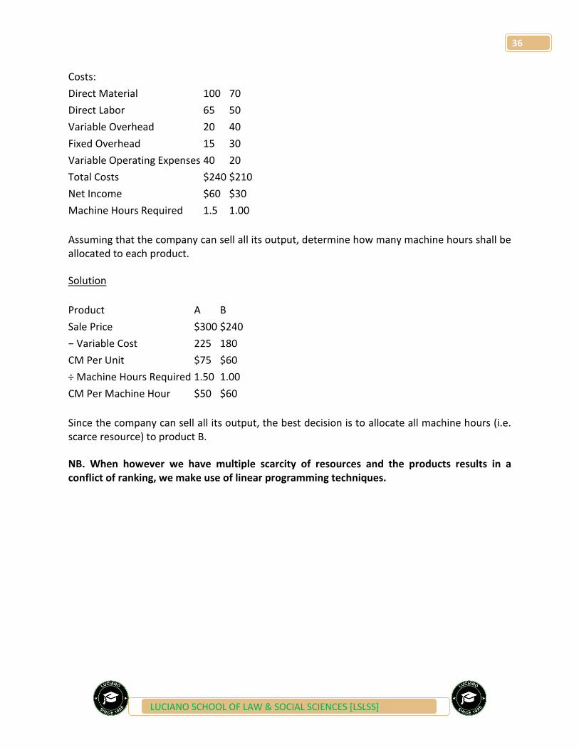
Total Costs $240 $210

Net Income $60 $30

Machine Hours Required 1.5 1.00

Assuming that the company can sell all its output, determine how many machine hours shall be allocated to each product.

Solution

Product A B

Sale Price $300 $240

− Variable Cost 225 180

CM Per Unit $75 $60

÷ Machine Hours Required 1.50 1.00

CM Per Machine Hour $50 $60

Since the company can sell all its output, the best decision is to allocate all machine hours (i.e. scarce resource) to product B.

NB. When however we have multiple scarcity of resources and the products results in a conflict of ranking, we make use of linear programming techniques.



37


PROCESS COSTING

Some companies have homogeneous or very similar products that are not made to order and are produced in large volumes. They continually process their product, moving it from one function to the next until it is completed. In these companies, the manufacturing costs incurred are allocated to the proper functions or departments within the factory process rather than to specific products. Examples of products that companies produce continuously are cereal, bread, candy, steel, automotive parts, chips, and computers. Companies that refine oil or bottle drinks and companies that provide services such as mail sorting and catalog order are also examples of continuous, homogeneous processing.

Joint products

Joint products are two or more products separated in the course of processing, each having a sufficiently high saleable value to merit recognition as a main product.

Joint products include products produced as a result of the oil-refining process, for example, petrol and paraffin.

Petrol and paraffin have similar sales values and are therefore equally important (joint) products.

By-products

By-products are outputs of some value produced incidentally in manufacturing something else (main products).

By-products, such as sawdust and bark, are secondary products from the timber industry (where timber is the main or principal product from the process).

Sawdust and bark have a relatively low sales value compared to the timber which is produced and are therefore classified as by-products



http://www.businessdictionary.com/definition/unit-cost.html

http://www.businessdictionary.com/definition/output.html

http://www.businessdictionary.com/definition/continuous-production.html

http://www.businessdictionary.com/definition/food.html

http://www.businessdictionary.com/definition/processing.html

http://www.businessdictionary.com/definition/petroleum.html

http://www.businessdictionary.com/definition/textile.html

http://www.businessdictionary.com/definition/industry.html

http://www.businessdictionary.com/definition/process.html

http://www.businessdictionary.com/definition/cost-center.html

http://www.businessdictionary.com/definition/total-cost.html

http://www.businessdictionary.com/definition/estimating.html

http://www.businessdictionary.com/definition/product.html

http://www.businessdictionary.com/definition/period.html

http://www.businessdictionary.com/definition/unit.html

http://www.businessdictionary.com/definition/production.html

http://www.businessdictionary.com/definition/cycle.html

http://www.businessdictionary.com/definition/charge.html

38


Treatment of joint costs

Accounting treatment for joint products

The distinction between joint and by-products is important because the accounting treatment of joint products and by-products differs.

Joint process costs occur before the split-off point. They are sometimes called pre-separation costs or common costs.

The joint costs need to be apportioned between the joint products at the split-off point to obtain the cost of each of the products in order to value closing inventory and cost of sales.

The basis of apportionment of joint costs to products is usually one of the following: o sales value of production (also known as market value) o production units o net realisable value.

Accounting treatment for by-products

As by-products have an insignificant value the accounting treatment is different.

The costs incurred in the process are shared between the joint products alone. The by-products do not pick up a share of the costs, like normal loss.

The sales value of the by-product at the split-off point is treated as a reduction in costs instead of an income, again just the same as normal loss.

If the by-product has no known value at the split-off point but does have a value after further processing, the net income of the by-product is used to reduce the costs of the process.



39


Net income (or net realisable value) = Final sales value - Further processing costs In some production processes, particularly in agriculture and natural resources, two or more products undergo the same process up to a split-off point, after which one or more of the products may undergo additional processing. An oil company drills for oil and obtains both crude oil and natural gas. A second-growth forest is harvested, and lumber of various grades are milled. A farmer maintains a herd of dairy cows, and after the cows are milked, the milk naturally separates into skim and cream or can be separated into various products characterized by the amount of milkfat. Some of these products then constitute raw materials in the manufacture of other products such as butter and cheese. Following are some important terms: Common costs: These costs cannot be identified with a particular joint product. By definition, joint products incur common costs until they reach the split-off point. Split-off point: At this stage, the joint products acquire separate identities. Costs incurred prior to this point are common costs, and any costs incurred after this point are separable costs. Separable costs: These costs can be identified with a particular joint product. These costs are incurred for a specific product, after the split-off point. The characteristic feature of joint products is that all costs incurred prior to the split-off point are common costs, and cannot be identified with individual products that are derived at split-off. Furthermore, the costs incurred by the dairy farmer to feed and care for the cows do not significantly affect the relative amounts of cream and skim obtained, and the costs incurred by the lumber company to maintain and harvest the second-growth timber do not significantly affect the relative quantities of lumber of various grades that are obtained. Reasons for Allocating Common Costs: Given the lack of a cause-and-effect relationship between the incurrence of common costs and the relative quantities of joint products obtained, any allocation of these common costs to the joint products is arbitrary. Consequently, there is no management accounting purpose served by the allocation of these common costs. Literally, there is no managerial decision that becomes better informed by such an allocation. Consider the possibilities: 1. Can the allocation of common costs prompt the manager to favor some joint products over other joint products and to therefore change the production process, and hence the quantities of joint products obtained? No. By definition, the relative quantities obtained from the joint process are inherent in the production process itself, and cannot be managed. In fact, the manager probably does have



40


strong preferences for some joint products over others (high-grade lumber over low-grade lumber; cream over skim milk), but the manager’s preferences are irrelevant. 2. Can the allocation of common costs prompt the manager to change the sales prices for the joint products, or to change decisions about whether to incur separable costs to process one or more of the joint products further? No. The decision to sell a joint product at split-off or to process it further depends only on the incremental costs and revenues of the additional processing, not on the common costs. In fact, the common costs can be considered sunk at the time the additional processing decision is made. As for pricing, most joint products are commodities, and producers are generally price-takers. To the extent that the producer faces a downward sloping demand curve, determining the optimal combination of price and production level depends on the variable cost of production, but this calculation would have to be done simultaneously for all joint products, in which case no allocation of common costs would be necessary. 3. Can the allocation of common costs inform the manager that the entire production process is unprofitable and should be terminated? For example, does this allocation tell the dairy farmer whether the farmer should sell the herd and get out of the dairy business? No. Such an allocation is unnecessary for the decision of whether to terminate the joint production process. For this decision, the producer can look at the operation in its entirety (total revenues from all joint products less total common costs and total separable costs). Yet despite the fact that allocating common costs to joint products serves no decision-making purpose, it is required for external financial reporting. It is necessary for product costing if we wish to honor the matching principle for common costs, because these common costs are manufacturing costs. For example, if the dairy sells lowfat milk shortly after split-off, but processes high milkfat product into cheese that requires an aging process, the allocation of common costs is necessary for the valuation of ending inventory (work-in-process for cheese) and the determination of cost-of-goods sold (lowfat milk).



41


Alternative Methods for Allocating Common Costs: Here are four methods of allocating common costs: 1. Physical measure: Using this method, some common physical measure is identified to describe the quantity of each product obtained at split-off. For example: the weight of the joint products, or the volume. Common costs are then allocated in proportion to this physical measure. This method presumes that the quantities of all joint products can be expressed using a common measure, which is not always the case. For example, crude oil is a liquid, while natural gas is, naturally, a gas, and volumes of liquids and gasses are not normally measured in the same units. 2. Sales value at split-off: If a market price can be established for the products that are obtained at split-off, common costs can be allocated in proportion to the sales value of the products at split-off. The sales value of each joint product is derived by multiplying the price per unit by the number of units obtained. For example, if the dairy farmer obtains 20 gallons of cream, and if cream can be sold for $3 per gallon, then the sales value for cream is $60. If the farmer also obtains 40 gallons of skim milk that sells for $2 per gallon, then the sales value of skim milk is $80. The total value of both products is $140, and 43% ($60 ÷ $140) of common costs would be allocated to all 20 gallons of cream. This method can be used whether or not one or more of the joint products are actually processed further, as long as a market price exists for the product obtained at split-off. In other words, even if the farmer does not sell any cream, but processes all of the cream into butter, the fact that there is a market price for cream is sufficient for the farmer to be able to apply this method of common cost allocation. 3. Net Realizable Value: The net realizable value of a joint product at split-off is the sales price of the final product after additional processing, minus the separable costs incurred during the additional processing. If the joint product is going to be sold at split-off without further processing, the net realizable value is simply the sales value at split-off, as in the previous method. Under the net realizable value method of common cost allocation, common costs are allocated in proportion to their net realizable values. As with the previous method, the allocation is based on the total value of all quantities of each joint product obtained (the net realizable value per unit, multiplied by the number of units of each joint product). 4. Constant Gross Margin Percentage: This method allocates common costs such that the overall gross margin percentage is identical for each joint product. The gross margin percentage is calculated as follows: Gross Margin Percentage = (Sales – Cost of Goods Sold) ÷ Sales Cost of Goods Sold for each product includes common costs and possibly some separable costs. The application of the Constant Gross Margin Percentage requires solving for the allocation of common costs that equates the Gross Margin Percentage across all joint products.



42


Conclusion: The choice of method for allocating common costs should depend on the ease of application, the perceived quality of information reported to external parties, and the perceived fairness of the allocation when multiple product managers are responsible for joint products. However, as discussed above, the allocation of common costs is arbitrary, and no method is conceptually preferable to any other method. All methods of allocating common costs across joint products are generally useless for operational, marketing, and product pricing decisions.

Relevant Costing

Relevant costing is a management accounting toolkit that helps managers reach decisions when they are posed with the following questions:

1. Whether to buy a component from an external vendor or manufacture it in house? 2. Whether to accept a special order? 3. What price to charge on a special order? 4. Whether to discontinue a product line? 5. How to utilize the scarce resource optimally?, etc.

Relevant costing is an incremental analysis which means that it considers only relevant costs i.e. costs that differ between alternatives and ignores sunk costs i.e. costs which have been incurred, which cannot be changed and hence are irrelevant to the scenario.

Example

Company A manufactures bicycles. It can produce 1,000 units in a month for a fixed cost of $300,000 and variable cost of $500 per unit. Its current demand is 600 units which it sells at $1,000 per unit. It is approached by Company B for an order of 200 units at $700 per unit. Should the company accept the order?

Solution



43


A layman would reject the order because he would think that the order is leading to loss of $100 per unit assuming that the total cost per unit is $800 (fixed cost of $300,000/1,000 and variable cost of $500 as compared to revenue of $700).

On the other hand, a management accountant will go ahead with the order because in his opinion the special order will yield $200 per unit. He knows that the fixed cost of $300,000 is irrelevant because it is going to be incurred regardless of whether the order is accepted or not. Effectively, the additional cost which Company A would have to incur is the variable cost of $500 per unit. Hence, the order will yield $200 per unit ($700 minus $500 of variable cost).

DEFINITION of 'Relevant Cost'

A managerial accounting term that is used to describe costs that are specific to management's decisions. The concept of relevant costs eliminates unnecessary data that could complicate the decision-making process.

INVESTOPEDIA EXPLAINS 'Relevant Cost'

Relevant costs are decision specific, meaning that a relevant cost may be important in one situation but irrelevant in another. Examples of when management uses relevant costs can be seen when it is determining whether to sell or keep a business unit, make or buy an item, or accept a special order.

Management accounting uses the following terms from economics:

Costs: Resources sacrificed to achieve a specific objective, such as manufacturing a particular product, or providing a client a particular service.

Sunk costs: These are costs that were incurred in the past. Sunk costs are irrelevant for decisions, because they cannot be changed.

Opportunity cost: The profit foregone by selecting one alternative over another. It is the net return that could be realized if a resource were put to its next best use. It is “what we give up” from “the road not taken.”



44


Relevant costs: These are costs that are relevant with respect to a particular decision. A relevant cost for a particular decision is one that changes if an alternative course of action is taken. Relevant costs are also called differential costs.

The following discussion elaborates on these definitions:

Costs:

Costs are different from expenses. Costs are resources sacrificed to achieve an objective. Expenses are the costs charged against revenue in a particular accounting period. Hence, “cost” is an economic concept, while “expense” is a term that falls within the domain of accounting.

Costs can be classified along the following functional dimensions:

1. The value chain. The value chain is the chronological sequence of activities that adds value in a company. For example, for a manufacturing firm, the value chain might consist of research & development, design, manufacturing, marketing and distribution.

2. Division or business segment: e.g., Chevrolet, Oldsmobile, G.M.C.

3. Geographic location.

Classification of costs according to the value chain is particularly important for financial reporting purposes, because for external reporting, only manufacturing costs are included in the valuation of inventory on the balance sheet. Non-manufacturing costs are treated as period expenses. To some extent, traditional management accounting systems have been influenced by external reporting requirements, and consequently, costing systems usually reflect this distinction between manufacturing and non-manufacturing costs.



45


Sunk Costs:

Sunk costs are costs that were incurred in the past. Committed costs are costs that will occur in the future, but that cannot be changed. As a practical matter, sunk costs and committed costs are equivalent with respect to their decision-relevance; neither is relevant with respect to any decision, because neither can be changed. Sometimes, accountants use the term “sunk costs” to encompass committed costs as well.

Experiments have been conducted that identify situations in which individuals, including professional managers, incorporate sunk costs in their decisions. One common example from business is that a manager will often continue to support a project that the manager initiated, long after any objective examination of the project seems to indicate that the best course of action is to abandon it. A possible explanation for why managers exhibit this behavior is that there may be negative repercussions to poor decisions, and the manager might prefer to attempt to make the project look successful, than to admit to a mistake.

Some of us seem inclined to consider sunk costs in many personal situations, even though economic theory is clear that it is irrational to do so. For example, if you have purchased a nonrefundable ticket to a concert, and you are feeling ill, you might attend the concert anyway because you do not want the ticket to go to waste. However, the money spent to buy the ticket is sunk, and the cost of the ticket is entirely irrelevant, whether it cost $5 or $100. The only relevant consideration is whether you would derive more pleasure from attending the concert or staying home on the evening of the concert.

Here is another example. Consider a student who is between her junior and senior year in college, deciding whether to complete her degree. From a financial point of view (ignoring nonfinancial factors) her situation is as follows. She has paid for three years of tuition. She can pay for one more year of tuition and earn her degree, or she can drop out of school. If her market value is greater with the degree than without the degree, then her decision should depend on the cost of tuition for next year and the opportunity cost of lost earnings related to one more year of school, on the one hand; and the increased earnings throughout her career that are made possible by having a college degree, on the other hand. In making this comparison, the tuition paid for her first three years is a sunk cost, and it is entirely irrelevant to her decision. In fact, consider three individuals who all face this same decision, but one paid $24,000 for three years of in-state tuition, one paid $48,000 for out-of-state tuition, and one paid nothing because she had a scholarship for three years. Now assume that the student who paid out-of-state tuition qualifies for in-state tuition for her last year, and the student who had the three-year scholarship now must pay in-state tuition for her last year. Although these three



46


students have paid significantly different amounts for three years of college ($0, $24,000 and $48,000), all of those expenditures are sunk and irrelevant, and they all face exactly the same decision with respect to whether to attend one more year to complete their degrees. It would be wrong to reason that the student who paid $48,000 should be more likely to stay and finish, than the student who had the scholarship.

Opportunity Cost:

The term opportunity cost is sometimes ambiguous in the following sense. Sometimes it is used to refer to the profit foregone from the next best alternative, and sometimes it is used to refer to the difference between the profit from the action taken and the profit foregone from the next best alternative.

Example: Tina has $5,000 to invest. She can invest the $5,000 in a certificate of deposit that earns 5% annually, for a first-year return of $250. Alternatively, she can pay off an auto loan on her car, which carries an interest rate of 7%. If she pays off the auto loan, she will save $350 (7% of $5,000) in interest expense. (In this context, a dollar saved is as good as a dollar earned.)

Question: What is Tina’s opportunity cost from investing in the certificate of deposit?

Answer: The opportunity cost is the “profit foregone” from the best action not taken. The payoff from the action not taken is clear: it is the $350 in interest expense avoided by paying off the loan. However, there is some ambiguity as to whether the opportunity cost is this $350, or the difference between the $350, and the $250 that would be earned on the certificate of deposit, which is $100.

This ambiguity is only a question of semantics with respect to the definition of opportunity cost; it does not create any ambiguity with respect to the information provided by the concept of opportunity cost. Clearly, the opportunity cost of paying off the auto loan implies that Tina is better off paying off the loan than investing in the certificate of deposit.



47


When opportunity cost is defined in terms of the difference between the two profits (the $100 in the above example), then the opportunity cost can be either positive or negative, and a negative opportunity cost implies that the action taken is better than all alternatives.

Relevant Costs:

Relevant costs are costs that change with respect to a particular decision. Sunk costs are never relevant. Future costs may or may not be relevant. If the future costs are going to be incurred regardless of the decision that is made, those costs are not relevant. Committed costs are future costs that are not relevant. Even if the future costs are not committed, if we anticipate incurring those costs regardless of the decision that we make, those costs are not relevant. The only costs that are relevant are those that differ as between the alternatives being considered.

Including sunk costs in a decision can lead to a poor choice. However, including future irrelevant costs generally will not lead to a poor choice; it will only complicate the analysis. For example, if I am deciding whether to buy a Toyota Camry or a Subaru Legacy, and if my auto insurance will be the same no matter which car I buy, my consideration of insurance costs will not affect my decision, although it will slightly complicate the analysis.

Microeconomic Analysis and the Matching Principle:

The matching principle (matching expenses with the associated revenues) provides useful information, if properly interpreted. However, there are ways in which the matching principle can obscure relevant costs. For example, to honor the matching principle, companies capitalize assets and depreciate them over their useful lives. In manufacturing companies, depreciation expense in any one year for assets used in production is allocated yet again, to individual products made during the period. The result is that the cost of each unit of product includes depreciation expense that represents the allocation of a cost that was probably incurred years ago. However, except for any tax implications that arise because depreciation expense reduces taxable income, depreciation expense should be ignored with respect to all decisions.

Concept

Relevant costing attempts to determine the objective cost of a business decision. An objective measure of the cost of a business decision is the extent of cash outflows that shall result from its implementation. Relevant costing focuses on just that and ignores other costs which do not affect the future cash flows.



48


The underlying principles of relevant costing are fairly simple and you can probably relate them to your personal experiences involving financial decisions.

For example, assume you had been talked into buying a discount card of ABC Pizza for $50 which entitles you to a 10% discount on all future purchases. Say a pizza costs $10 ($9 after discount) at ABC Pizza and it subsequently came to your knowledge that a similar pizza is offered by XYZ Pizza for just $8. So the next time you would have ordered a pizza, you would have (hopefully) placed an order at XYZ Pizza realizing that the $50 you have already spent is irrelevant (see sunk cost below).

Relevant costing is just a refined application of such basic principles to business decisions. The key to relevant costing is the ability to filter what is and isn't relevant to a business decision.

Types of Relevant Costs Types of Non-Relevant Costs

Future Cash Flows Cash expense that will be incurred in the future as a result of a decision is a relevant cost.

Sunk Cost Sunk cost is expenditure which has already been incurred in the past. Sunk cost is irrelevant because it does not affect the future cash flows of a business.

Avoidable Costs Only those costs are relevant to a decision that can be avoided if the decision is not implemented.

Committed Costs Future costs that cannot be avoided are not relevant because they will be incurred irrespective of the business decision bieng considered.

Opportunity Costs Cash inflow that will be sacrificed as a result of a particular management decision is a relevant cost.

Non-Cash Expenses Non-cash expenses such as depreciation are not relevant because they do not affect the cash flows of a business.

Incremental Cost Where different alternatives are being considered, relevant cost is the incremental or differential cost between the various alternatives being considered.

General Overheads General and administrative overheads which are not affected by the decisions under consideration should be ignored.

Example



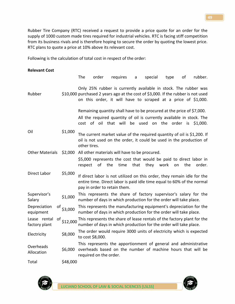
49


Rubber Tire Company (RTC) received a request to provide a price quote for an order for the supply of 1000 custom made tires required for industrial vehicles. RTC is facing stiff competition from its business rivals and is therefore hoping to secure the order by quoting the lowest price. RTC plans to quote a price at 10% above its relevant cost.

Following is the calculation of total cost in respect of the order:

Relevant Cost

Rubber $10,000

The order requires a special type of rubber. Only 25% rubber is currently available in stock. The rubber was purchased 2 years ago at the cost of $3,000. If the rubber is not used on this order, it will have to scraped at a price of $1,000. Remaining quantity shall have to be procured at the price of $7,000.

Oil $1,000

All the required quantity of oil is currently available in stock. The cost of oil that will be used on the order is $1,000. The current market value of the required quantity of oil is $1,200. If oil is not used on the order, it could be used in the production of other tires.

Other Materials $2,000 All other materials will have to be procured.

Direct Labor $5,000

$5,000 represents the cost that would be paid to direct labor in respect of the time that they work on the order. If direct labor is not utilized on this order, they remain idle for the entire time. Direct labor is paid idle time equal to 60% of the normal pay in order to retain them.

Supervisor's Salary

$1,000 This represents the share of factory supervisor's salary for the number of days in which production for the order will take place.

Depreciation of equipment

$3,000 This represents the manufacturing equipment's depreciation for the number of days in which production for the order will take place.

Lease rental of factory plant

$12,000 This represents the share of lease rentals of the factory plant for the number of days in which production for the order will take place.

Electricity $8,000 The order would require 3000 units of electricity which is expected to cost $8,000.

Overheads Allocation

$6,000 This represents the apportionment of general and administrative overheads based on the number of machine hours that will be required on the order.

Total $48,000



50


Calculate the relevant cost for the order and the price RTC should quote.

Manufacturing Cost

Rubber $8,000

25% - Scrap Value $1,000 75% - Purchase Cost $7,000 Relevant Cost $8,000 The $3,000 paid two years ago is a sunk cost and should therefore be ignored. $1,000 represents the opportunity cost of using the rubber available in stock on this particular order.

Oil $1,200

The $1,000 cost of oil is a sunk cost. The $1,200 current market value of the required oil is the relevant cost because utilizing it on this order will require purchase of additional oil at the market rates to meet the production needs of other tires. Alternatively, the oil could be sold for $1200.

Other Materials $2,000 As these materials are not available in stock, these will have to be purchased at the market price which is their relevant cost.

Direct Labor $2,000 Since $3,000 (60% of $5,000) idle time pay will be incurred even if this order is not taken, the relevant cost is the incremental cost of $2,000 ($5,000 - $3,000).

Supervisor's Salary

- As supervisor's salary is a fixed cost unchanged by the work performed on this order, it is a non-relevant cost.


- Non-cash expenses are not relevant for decision making.


- Lease rentals are a committed cost which cannot be avoided by withdrawing from this order which is why they should be ignored for the purpose of this analysis.

Electricity $8,000 Electricity charges are incremental to this order and therefore relevant.


- General and administrative overheads that are not incurred directly as a result of this order should be considered irrelevant.

Relevant Cost of order

$21,200

Profit Margin $2,120 10% of the relevant cost of $21,200

Price to be quoted

$23,320



51


Application & Limitations

While relevant costing is a useful tool in short-term financial decisions, it would probably not be wise to form it as the basis of all pricing decisions because in order for a business to be sustainable in the long-term, it should charge a price that provides a sufficient profit margin above its total cost and not just the relevant cost.

Examples of application of relevant costing include:

Competitive pricing decisions Make or buy decisions Further processing decisions

For long term financial decisions such as investment appraisal, disinvestment and shutdown decisions, relevant costing is not appropriate because most costs which may seem non-relevant in the short term become avoidable and incremental when considered in the long term. However, even long term financial decisions such as investment appraisal may use the underlying principles of relevant costing to facilitate an objective evaluation.

Concept Relevant costing attempts to determine the objective cost of a business decision. An objective measure of the cost of a business decision is the extent of cash outflows that shall result from its implementation. Relevant costing focuses on just that and ignores other costs which do not affect the future cash flows. The underlying principles of relevant costing are fairly simple and you can probably relate them to your personal experiences involving financial decisions. For example, assume you had been talked into buying a discount card of ABC Pizza for $50 which entitles you to a 10% discount on all future purchases. Say a pizza costs $10 ($9 after discount) at ABC Pizza and it subsequently came to your knowledge that a similar pizza is offered by XYZ Pizza for just $8. So the next time you would have ordered a pizza, you would have (hopefully) placed an order at XYZ Pizza realizing that the $50 you have already spent is irrelevant (see sunk cost below). Relevant costing is just a refined application of such basic principles to business decisions. The key to relevant costing is the ability to filter what is and isn't relevant to a business decision.

Types of Relevant Costs Types of Non-Relevant Costs

Future Cash Flows Cash expense that will be incurred in the future as a result of a decision is a relevant cost.

Sunk Cost Sunk cost is expenditure which has already been incurred in the past. Sunk cost is irrelevant because it does not affect the future cash flows of a business.

Avoidable Costs Committed Costs



52


Only those costs are relevant to a decision that can be avoided if the decision is not implemented.

Future costs that cannot be avoided are not relevant because they will be incurred irrespective of the business decision bieng considered.

Opportunity Costs Cash inflow that will be sacrificed as a result of a particular management decision is a relevant cost.

Non-Cash Expenses Non-cash expenses such as depreciation are not relevant because they do not affect the cash flows of a business.

Incremental Cost Where different alternatives are being considered, relevant cost is the incremental or differential cost between the various alternatives being considered.

General Overheads General and administrative overheads which are not affected by the decisions under consideration should be ignored.

Example Rubber Tire Company (RTC) received a request to provide a price quote for an order for the supply of 1000 custom made tires required for industrial vehicles. RTC is facing stiff competition from its business rivals and is therefore hoping to secure the order by quoting the lowest price. RTC plans to quote a price at 10% above its relevant cost. Following is the calculation of total cost in respect of the order:

Relevant Cost

Rubber $10,000

The order requires a special type of rubber. Only 25% rubber is currently available in stock. The rubber was purchased 2 years ago at the cost of $3,000. If the rubber is not used on this order, it will have to scraped at a price of $1,000. Remaining quantity shall have to be procured at the price of $7,000.

Oil $1,000

All the required quantity of oil is currently available in stock. The cost of oil that will be used on the order is $1,000. The current market value of the required quantity of oil is $1,200. If oil is not used on the order, it could be used in the production of other tires.

Other Materials $2,000 All other materials will have to be procured.

Direct Labor $5,000 $5,000 represents the cost that would be paid to direct labor in respect of the time that they work on the order.



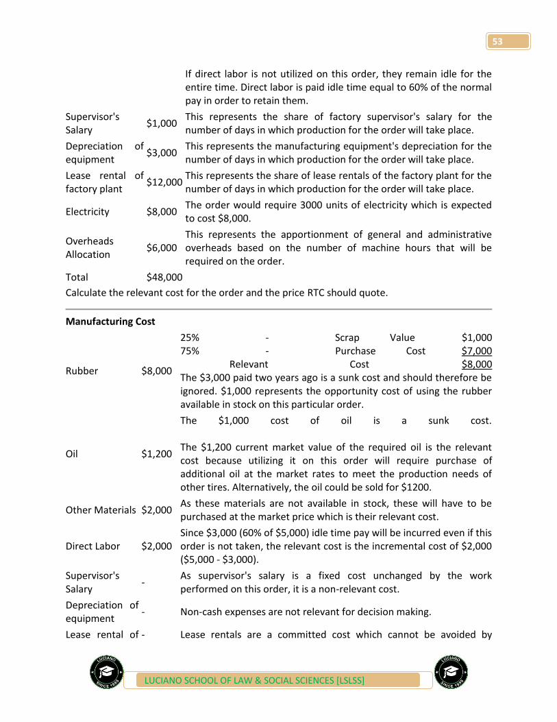
53


If direct labor is not utilized on this order, they remain idle for the entire time. Direct labor is paid idle time equal to 60% of the normal pay in order to retain them.

Supervisor's Salary

$1,000 This represents the share of factory supervisor's salary for the number of days in which production for the order will take place.


$3,000 This represents the manufacturing equipment's depreciation for the number of days in which production for the order will take place.


$12,000 This represents the share of lease rentals of the factory plant for the number of days in which production for the order will take place.

Electricity $8,000 The order would require 3000 units of electricity which is expected to cost $8,000.


$6,000 This represents the apportionment of general and administrative overheads based on the number of machine hours that will be required on the order.

Total $48,000

Calculate the relevant cost for the order and the price RTC should quote.

Manufacturing Cost

Rubber $8,000

25% - Scrap Value $1,000 75% - Purchase Cost $7,000 Relevant Cost $8,000 The $3,000 paid two years ago is a sunk cost and should therefore be ignored. $1,000 represents the opportunity cost of using the rubber available in stock on this particular order.

Oil $1,200

The $1,000 cost of oil is a sunk cost. The $1,200 current market value of the required oil is the relevant cost because utilizing it on this order will require purchase of additional oil at the market rates to meet the production needs of other tires. Alternatively, the oil could be sold for $1200.

Other Materials $2,000 As these materials are not available in stock, these will have to be purchased at the market price which is their relevant cost.

Direct Labor $2,000 Since $3,000 (60% of $5,000) idle time pay will be incurred even if this order is not taken, the relevant cost is the incremental cost of $2,000 ($5,000 - $3,000).

Supervisor's Salary

- As supervisor's salary is a fixed cost unchanged by the work performed on this order, it is a non-relevant cost.


- Non-cash expenses are not relevant for decision making.

Lease rental of - Lease rentals are a committed cost which cannot be avoided by



54


factory plant withdrawing from this order which is why they should be ignored for the purpose of this analysis.

Electricity $8,000 Electricity charges are incremental to this order and therefore relevant.


- General and administrative overheads that are not incurred directly as a result of this order should be considered irrelevant.

Relevant Cost of order

$21,200

Profit Margin $2,120 10% of the relevant cost of $21,200

Price to be quoted

$23,320

Application & Limitations While relevant costing is a useful tool in short-term financial decisions, it would probably not be wise to form it as the basis of all pricing decisions because in order for a business to be sustainable in the long-term, it should charge a price that provides a sufficient profit margin above its total cost and not just the relevant cost. Examples of application of relevant costing include:

Competitive pricing decisions Make or buy decisions Further processing decisions

For long term financial decisions such as investment appraisal, disinvestment and shutdown decisions, relevant costing is not appropriate because most costs which may seem non-relevant in the short term become avoidable and incremental when considered in the long term. However, even long term financial decisions such as investment appraisal may use the underlying principles of relevant costing to facilitate an objective evaluation. Business owners faced with tough decisions can use one or both of two general approaches to problem solving. The qualitative approach draws on a manager’s experience and expertise, which together hone keen business instincts concerning the likelihood of success. The quantitative approach is more formal. Using mathematical reasoning, a manager derives the solution on paper and puts it into practice.



55


QUALITATIVE DECISION MAKING:

The qualitative approach requires experiential knowledge of the various factors involved in a decision. For example, to use the qualitative approach to solve a dispute over resources between two departments of an organization, the manager must understand the complex interplay of variables in that organization, such as the interpersonal connections among supervisors in each department and the overall availability of resources for which the two departments are competing. In simpler terms, the manager must have an intuitive feel for how decisions will play out given the nature of that organization, which can only come from direct, hands-on experience.

Managers lacking direct experience can opt for a quantitative approach. The first step is to translate the problem into mathematical language. Accordingly, the quantitative approach works best for objectively measurable problems. For example, deciding how to distribute resources among many departments might begin with determining which departments are the most profitable and therefore most likely to generate more profits per unit of fresh resources. Based on this reasoning, the manager uses accounting data to construct a mathematical model, or formula, for resource apportionment.

Quantitative models can fail because a manager over- or underestimates, or entirely fails to account for, an important variable. For example, relying on the relative profitability of various departments to apportion resources doesn’t account for scalability. Some of the top-producing departments might be operating at peak efficiency; more resources won’t generate proportionally more profits because the employees simply can’t work any faster.

Illogic can cripple either approach, but the quantitative approach is more vulnerable because it relies so heavily on formal reasoning. Therefore, close monitoring of results is vital to verify the reasoning behind a quantitative decision. In contrast, managers using the qualitative approach likely have fair expectations for how their decisions will play out due to past experiences in similar situations.

Use both approaches, if possible. Combining depth of experience with keen mathematical reasoning to make a tough decision offers a better chance of success than either would separately. Each element complements the other, creating maximally efficient and effective solutions to difficult problems.

Daily activities are the result of our decisions. Most of our crucial decisions are intuitive, based on our personality, accumulated experience, knowhow and environment. We refer to these decisions as Qualitative Decisions. We developed a unique expertise to improve qualitative decision making while differentiating these from quantitative decision making. Qualitative Decisions are hard to quantify at the time these are made. Business visions,



56


Homeland Security issues, personal decisions are all qualitative decisions. Entrepreneurs succeed because of visions, leadership and determination. Scientific breakthroughs reflect the scientists' ability to think in ever wider terms. Companies, through their managing individuals, have chosen to take business risks achieving huge returns, while others decided to put aside integrity leading their companies to ruin. Homeland security concepts are as good as the designers' ability to think as a perpetrator. Many examples are there, in all aspects of life, of how qualitative decisions proved decisive in shaping the future of businesses, medicine, agriculture, security and many other disciplines. Once made, Qualitative decisions are quantified for execution and control purposes to the point that organizations concentrate on executing measurable activities, while visions and strategies tend to lag behind.

In cost accounting, qualitative factors don’t involve numbers and financial analysis. Call them “people” factors. Decisions based in part on qualitative factors are relevant, even though you can’t tie specific cost or revenue numbers to them. They can have a long-term impact on profitability, so you need to consider them. Qualitative factors should always be considered before making any business decisions.

The qualitative factor that has the biggest impact on your business may be employee morale. It’s really an issue when there’s bad news, such as a layoff. Layoffs, as a rule, don’t improve employee morale. Employees are uncertain about their futures, even if they’ve been told that their jobs are secure. They may be skeptical, saying, “Yeah, and if you believe that, I’ve got a bridge I want to sell you.”

On top of that, the remaining employees may have to take on the workload of people who were let go. The worst thing you can say to them is, “Work smarter, not harder.” Employees have a BS meter that’s always operating, and that statement is a 9.9 on a scale of 10.

There’s a rule that’s true far more often than not: When employee morale goes down, productivity goes down, too.

When companies reduce the workforce, the goal is to reduce costs. If a firm has 100 employees and cuts the staff to 80 people, you’d think profits would go up. The company cut the cost (salary and benefits) of 20 people. The problem occurs with the remaining 80 people. Productivity (how much they get done) suffers in the short term. Also, most people have an emotional reaction to the layoff. That emotion affects productivity.

There’s another, bigger potential problem with layoffs: When you lay people off, some institutional knowledge leaves with them. Even the best operations manual can’t cover everything. If a company lays off a great sales representative, personal relationships with customers may suffer, too.



57


When other key people leave, those taking up their duties will make mistakes — that’s almost unavoidable. Those mistakes can cost the company business, if the company isn’t careful. In extreme situations, lost business (due to mistakes) costs more than the cost savings from the layoff.

You may not be able to trace the impact of a qualitative factor such as layoff effects to product costs, but you can allocate it. Doing so adds more lines to your decision-making analysis. It also requires you to make judicious estimates. For example, you might say, “I’m going to assume a 10 percent drop in productivity for three months.”

The remainder of the decision-making process is simple but requires some detail work. First, implement your decision. Then evaluate the outcome of your decision. The results will tell you if you decided wisely. If you’ve made a mistake, you must make new decisions about how to fix it.



58


FEEDBACK FROM PAST PAPERS

MAY/JUNE 2014



59




60




61




62




63




64




65




66




67




68




69




70


ADDITIONAL QUESTIONS

Set one



71




72




73




74




75




76




77




78


Answers to Set One Questions



79




80




81




82




83




84




85




86




87




88




89




90




91




92




93




Documents

EXAMPACK - Unisa Study Notesgimmenotes.co.za/.../12/mac3701-exampack-2015-edition.pdfSTUDY NOTES..... 3 STANDARD COSTING AND VARIANCE ANALYSIS..... 15 Cost Volume Profit Analysis