Examining the Possibility of Fuzzy Set Theory Application in

Journal of the Eastern Asia Society for Transportation Studies, Vol. 8, 2010

Examining the Possibility of Fuzzy Set Theory Application in Travel Demand Modelling

Gusri YALDI Michael A P TAYLOR PhD Student Professor of Transport Planning ISST-Transport Systems Director - ISST University of South Australia University of South Australia Adelaide, South Australia, SA 5001 Adelaide, South Australia, SA 5001 Fax: +61 8 8302 1880 Fax: +61 8 8302 1880 E-mail: [email protected] E-mail: [email protected] Wen Long YUE Senior Lecturer, Program Director ISST-Transport Systems University of South Australia Adelaide, South Australia, SA 5001 Fax: +61 8 8302 1880 E-mail: [email protected] Abstract: The sources of errors in travel demand model output are not only from a lack of information related to the parameters that the model tries to estimate but also due to the absence of sharply defined criteria of class membership that can play important roles in human thinking, for which qualitative variables may be better representations. Fuzzy Set Theory (FST) is suggested as an approach to tackle the computation of such variables. Combined with other approaches, in this case Artificial Neural Network (NN) and Doubly Constrained Gravity (DCG), the FST is used to model intra city work trip distribution with trip length addressed as a fuzzy attribute. However, the fuzzy model tends to perform with the same level of accuracy as un-combined models. In some cases, the hybrid models have a slightly lower performance than NN and DCG. Findings from this study suggest that FST may be suitable for inter city trip, but not short trip distribution model. Key Words: Fuzzy Set Theory, Artificial Neural Network, Doubly Constrained Gravity Model 1. INTRODUCTION Modelling in transport system planning has important roles to play. According to Hensher and Button (2000) the role of modelling is essential in most decision-making processes. The impacts of changes in the systems can be predicted through a model, providing a cheaper alternative when compared to the impact investigation after the changes are directly applied to the systems. A travel demand model is an important tool for forecasting the impact of the changes in operating characteristics on the usage of the transport networks, either now or in the future. The result is used to enhance the existing service quality by, for example, modifying the use of available services or providing new infrastructure facilities. For the latter purpose, the result is used to plan and evaluate each proposed alternative solution before selecting the best


option. In conventional transportation planning practice the model has generally been subdivided into (1) Trip Generation, (2) Trip Distribution, (3) Mode Choice, and (4) Traffic Assignment. This study focuses on trip distribution only, especially intra city work trip. Development in travel demand modelling often involved the application of theories from other disciplines such as economies, information technology and even biology in order to maintain the behavioural basis and to simplify the model, and to obtain better results. Fuzzy Set Theory (FST), originally from the information technology discipline, is one of them. As travel demand modelling can be related to the decision-making by humans, the process of which often use natural languages (qualitative variables) to communicate amongst them, FST is claimed to be able to tackle such variables. The natural language is characterized by uncertainty, ambiguity and imprecision that conventional probability theory is unable to capture. Thus, FST is potentially a powerful tool in dealing with uncertainty related to the semantic meaning of events, phenomena or statements that often occur in transport systems (Teodorovic and Vukadinovic, 1998, Zimmermann, 1991). Our literature review suggests that FST application in travel demand modelling is continuously growing. FST is claimed to compute the qualitative variables more accurately than assigning arbitrary numbers for such variables. However, the FST cannot model the demand by itself. It needs to be combined with other method(s), for example, studies conducted by Yin et al. (2002), Aldian (2003), Aldian & Taylor (2003), and Dell’Orco et al. (2007). Yin et al. (2002) used the Fuzzy approach combined with Artificial Neural Network (NN). FST approach was used in grouping traffic patterns into similar cluster based on its characteristics determined through its degree membership values, NN approach was used in specifying input and output relationship in the same way as conventional NN. The hybrid approach was found effective and more accurate than a conventional NN model. Aldian (2003) used Fuzzy Multicriteria analysis to calculate the aggregate utilities (trip production power and attractiveness) of inter city trip distribution model. The FST was used to calculate the crisp score of the attributes that construct the road user cost between an origin and a destination. There were three attributes, namely (1) Trip length/Distance, (2) Road geometry, and (3) Ride quality. The application of FST improved the model coefficient of determination by double that of the traditional model. Another study by Aldian and Taylor (2003) also suggested that use of FST combined with traditional trip generation model could improve the model coefficient of determination by factor of two. One of the fuzzy attributes in that study was also the distance/trip length. For mode choice study, Dell’Orco et al. (2007) is a good example. They used FST combined with the Random Utility Theory/Discrete choice model in estimating the proportion of travellers choosing a particular transit/public transport among three alternatives with single utility criteria, in this case travel time. Travel time was assumed as a fuzzy criterion representing the users’ uncertainty and vagueness. Thus, the travel time is presented in term of numeric interval such as left limit value, central value and right limit value. Hence, the study may be considered as a combination of random and fuzzy theories. A method to calculate the unique probability is also presented. Dell’Orco et al. (2007) termed this the hybrid approach.


The results were compared to the traditional Logit model. It was found that the hybrid model generated results fitted to the experimental data and with a significant level higher than that for the Logit model. However, there was a difference in the chosen alternative rank. The hybrid model gave the same rank or order in term of proportion to choice behaviour survey of the participants, but the Logit model did not, even though the first/the highest alternative is the same. Although various studies demonstrated the advantages of FST in improving the model performance, there is no study so far that used FST in intra city trip distribution, especially work trips. This paper is aimed at investigating the possibility of modelling intra city work trip distribution combining FST with two different trip distribution modelling methods, namely doubly constrained gravity (DCG), called the Fuzzy Gravity model (FG), and Artificial Neural Network, named the Fuzzy Neuro model (FN). The independent variables for NN (the input nodes) are the same as the DCG. Those are trip production (P), trip attraction (A) and trip length/distance (D). The dependent variable is trip flow (Tij). The trip length here is addressed as a fuzzy attribute as used by Aldian (2003) and Aldian & Taylor (2003). However, they used the distance multiplied with other attributes (ride quality and road geometry) to calculate the road user cost for intercity trip generation and trip production models. According to Aldian & Taylor (2003), distance is a fuzzy attribute because the following facts, namely (1) Most travellers would not know the exact distance travelled from origins and destinations, and (2) Each traveller starts to travel from different points within an origin zone to different points in the destination zone. These considerations can also be applicable to the commuter trips such as work trip where the trip makers start their journey from different locations in the same origin zones to different locations in the same destination zones. Therefore, fuzzy attribute is used to represent such incomplete/imprecise variable. The Chen and Hwang (1992) method was used to calculate the crisp value of the fuzzy attribute. The fuzzy distance was divided into 29 categories based on the trip length data. More details regarding fuzzy attribute scoring is given in the second half part of the paper. Meanwhile, the DCG was used in this study because it is known as the best traditional method for modelling work trip distribution, and is widely used. The NN approach is used in various studies in transportation area provides evidences of the advantages of this technique compared with existing methods in the relevant studies. For example, multilayer perceptron neural network has been compared with Discrete Choice Model (DCM) for mode choice study as reported by Cantarella & de Luca (2005), Hensher & Ton (2000), Carvalho et al. (1998), and Subba Rao et al. (1998). There is less reported application of NN in trip distribution compared to mode choice study. Black (1995) reported a study of spatial interaction modelling using NN focusing on commodity flows. The model was structured based on the doubly constrained gravity model (DCG) and named as Gravity Artificial Neural Network (GNN). For passenger flow modelling, Mozolin et al. (2000) is a good example. They used NN to model trip distribution which is also characterized by DCG. Both studies reported promising results. Originally from Biology, NN is gradually being adopted in many studies, including travel demand modelling due to the following reasons: (1) Powerful pattern classification and pattern recognition, (2) Ability to learn and generalize from experience, (3) Ability to learn


from example, and (4) Ability to capture the functional relationships among data even if the underlying relationships are unknown or hard to describe (Teodorovic and Vukadinovic, 1998). Therefore, combining NN with FST is expected to improve the model performance more than the NN itself. In case of DCG, it is also expected the FST can lift the accuracy of the overall model. The performance of NN is characterized by its important properties, such as learning algorithm, activation function, number of layers, number of nodes inside each layer, and learning rate (Teodorovic and Vukadinovic, 1998, Dougherty, 1995). The amount of dataset and the ratio for training, validating and testing is also important for the NN fitting performance (Carvalho et al., 1998). Back-Propagation with momentum is the learning algorithm used in this study, while Sigmoid function (Logsig) is the activation function. The remaining properties need to be found through a trial and error procedure as the guideline does not exist so far (Zhang et al., 1998). There are three different learning rates, various hidden layer nodes starting from one to twenty nodes and five different percentages of dataset for training, validation and testing used in this study. Therefore, there are total one hundred scenarios used in this study. The purpose of using that number of scenarios is to define the ability of FST in improving the NN model with various modifications on its properties. Thus, the consistency of the model performance can be evaluated. For the DCG models, the trip distribution was calibrated using Hyman’s algorithm (Hyman, 1969). The model was calibrated with two different deterrence functions, namely Negative Exponential and Negative Power functions. We used the same data as NN models to calibrate and to test the gravity model. To measure the model performance, Root Mean Square Error (RMSE) was used. Two kinds of t-test, namely (1) One-Sample t-test and, (2) Paired t-tests, were used to evaluate the performance of each model. Overall, the NN performs at the same level as the DCG models. The hybrid models (FN), tends to perform as good as the NN models. The FG model has very much the same results as DCG models; therefore the FN model also performs the same level as the NN models. It is suggested that the FST approach cannot improve both NN and DCG model performance for short term work trip distribution modelling, and hence unsuitable to combine with them. The following section describes the model development for both NN and DCG, scoring the fuzzy distance attributes, discussion on the model performance and conclusions. 2. MODEL DEVELOPMENT 2.1 NN and FN Model Structures The structure of the NN model is one of its important properties. Multilayer perceptron neural network is commonly used in many studies, which is also used here. It has three layers, namely input, output and hidden layers. Each layer has a number of nodes or processing units. Except for hidden layer nodes, the numbers of processing units are determined by the variables that construct the expected outputs.


The doubly-constrained Gravity model is widely known and used to model trip distribution when both trip production and trip attraction totals are known. The NN structure, it is analogue to doubly constrained gravity model. The trip flow is a function of trip production, trip attraction and trip length as the deterrence factor. Therefore, there are three nodes at the input layer, while output layer has only one node. The number of hidden layer node is obtained through trial and error. It is started from one to twenty nodes (Figure 1.a). The proposed fuzzy-neuro model structure for trip distribution is illustrated by Figure 1.b. There are also three input nodes as NN model. The difference is in the trip length, where the distance is processed as a fuzzy attribute. The output is the trip flow from specified origins and destinations.

(a) (b)

Figure 1 NN and FN model structures 2.2 Learning Rate The role of learning rate is to determine how much the layer weight should be adjusted on each calibration process. In order to find the value of learning rate that can give the best performance of the network, three different values were used. Those are 0.1, 0.01 and 0.001. Those values are chosen as suggested by literature review where there is no standard value for that. It is usually a small positive value, below one. 2.3 Hidden layer node Unlike other layers, the number of nodes in hidden layer(s) is determined through a series of experiments. To investigate the relationship between numbers of nodes in hidden layer, various networks were developed with number of nodes starting from one to twenty nodes. There is no literature so far suggested the relationship between node numbers and model performance. However, the higher numbers of node will lengthen the calibration/training time. 2.4 Data for Training, Validation and Testing The study used work trip data collected by Transportation Agent of Padang City, West Sumatra, Indonesia. It was collected in 2003. Work trips formed about 16 per cent of total

A

A

wk‐j

wj‐i

A

Tij

P

A

A

wk‐j

wj‐i

A

Tij

P D

Journal o

trips (Fnodes insamples The guifar. Howfactors divisionselectedvalidatedifferen

No. DT

1* 2* 3* 4 5

* = vali 2.5 OthMaximufor netwThe epo The mo7.0.1. Twere upwas me There awith leasame mother NN

of the Eastern A

igure 2). Tn input ands.

idance in divwever, the pconsidered

ns used in thd. The first ed. The lastnt data divis

Data percentagTraining V

60 60 60 60

100 dated netwo

her Propertum number works with voch is also l

odel was deThe initial wpdated afterasured usin

are 100 NN arning rate

model with lN models. T

Asia Society f

T

There are 36d output lay

viding the dproblem chin making

he study (Tthree modet two modeion for train

Figure

Tge (%)

Validation 10 30 40

None None

orks/models

ties of epoch w

validation simited to pr

veloped byweights for r all of the ng Root Mea

models tra0.1 startingearning rateThere are al

for Transporta

Othe55%

Trip percentag

6 traffic anyers. Those

data sets intaracteristicsdata divisio

Table 1). Daels are categels are thenning, valida

e 2 Trip per

Table 1 Data

Testing

The sam

The ss

was set as 50sample; the revent over

y using the Nall layers wdata are usean Square E

ined using g from hiddees of 0.01 also 100 FN

ation Studies,

er%

ge based on pu

alysis zonedata are div

to developins, data typeon (Zhang eata for trainigorized as vn categorizeation and tes

rcentage bas

a division fo

me as validatio

ame as trainin

00 iterationstraining wafitting.

Neural Netwwere randomed in the tr

Error (RMSE

MATLAB en layer noand 0.001. Tmodels, tra

Vol. 8, 2010

Wo16

Shop9

urpose-year 2

es. Hence, tvided into t

ng and evalue and the sizet al., 1998)ing, validatvalidated med as un-vasting will be

sed on purpo

for NN modRem

30 10

on data 40

ng data

s. It is basedas always st

work Tool mly selectedraining (batcE).

software. Wode of 1 to 2The same pained by the

ork6%

School20%

pping9%

003

there are 12training, va

uating sampze of the av). There areion and test

models sincealidated one discussed

ose (2003)

el mark

Called aCalled aCalled Called

Call

d on our exptopped with

in MATLAd by the sofch mode). M

We firstly tr20. Then, itrocedures w same proce

296 samplealidation and

ple does notvailable datae five differting were ra

e the networes. The imlater in this

as 601030 moas 603010 moas 6040V moas 6040T mo

led as 100 mo

perience, esh epochs bel

AB softwareftware. The Model perfo

rain 601030t is followewere undertedures as N

es for all d testing

t exist so a are the rent data andomly rks were

mpacts of s paper.

odel odel odel odel odel

specially low 500.

e version weights

formance

0 models ed by the taken for

NN.


2.6 DCG and FG Models The gravity model was calibrated and tested with the same data as NN model with 100 per cent data sample. Hyman’s algorithm was used to calibrate the model as it is known as a robust maximum likelihood method for calibration. Two different deterrence functions were used, namely negative exponential and negative power functions. The formula to estimate the flow is given below.

(1) With the constraints of: ∑ (2) And ∑ (3) The travel impedance f(cij), is a generalized function of the travel costs with one calibration parameter. We used negative exponential function (e-βcij) and negative power function (cij-n). Trip length (distance/D) is used as deterrence function variable. Here, trip length is assumed as a fuzzy attribute and represented by ( ) for FG models. Developing FG models have basically the same procedures as the convention model; however, the deterrence function is based on fuzzy distance. The trip length is considered as a fuzzy attribute. There are 29 categories of distances based on the trip length data (Table 2). Next section will discuss the process of converting fuzzy attribute to crisp score. 3. SCORING FUZZY DISTANCE Fuzzy set theory firstly introduced by Zadeh (1965). It provides a framework in classifying imprecise objects/criteria into a continuum of grades of memberships. The imprecision occurs due to the absence sharply undefined criteria of class membership rather than the presence of random variables and it plays important role in human thinking (Zadeh, 1965). In classic set theory, memberships are categorised as binary membership function. There are only two options such as yes or not, true or false, ‘belongs to’ or ‘not belongs to’ a set. The membership function is defined by crispy or precise character and given by the equation below (Teodorovic and Vukadinovic, 1998). 1, 0, (4)

On the other hand, a fuzzy set A is represented by order pairs “A = (x, µA(x)”, where µA(x) is the grade of membership of element x in set A. Each element in a fuzzy set is labelled with certain grade of membership. The grade membership has a value from zero to one, i.e. a value from the closed interval [0, 1]. The greater µA(x), the greater the truth of the statement that


element x belongs to set A. As fuzzy sets are commonly defined by membership functions, each fuzzy set must comply with the condition below. 0 1 (5) The membership value must be converted to a crisp score before being used in final computation. This process is relatively simple. Various methods are available, such as dominance, maximin, maximax, and conjunctive methods (Hwang and Yoon, 1979). In this study, we used a method proposed by Chen & Hwang (1992). The crisp score is obtained by maximizing set and minimizing set techniques. Triangular membership function is used to represent the fuzzy number in this study Figure 3). The following conditions and equations define the membership functions and calculate the crisp score for fuzzy attributes. , 0 10, (6) 1 , 0 10, (7) To compute the total score of a fuzzy number A , the following formula is used. 1 /2 (8) Where is the right score and is the left score. The scores are calculated as the intersection between the fuzzy numbers and the minimizing/maximizing sets. For the left score, it is the intersection with the minimizing set (diagonal solid line) and left size of the fuzzy number. The intersection between maximizing set (diagonal broken line) and right side of the fuzzy number represent the right score (Figure 3). We used 29 fuzzy numbers for distance based on the trip length data. This is almost triple than the scales suggested by Chen and Whang (1992). The number of categories is relatively high as there are 36 traffic analysis zones with the minimum trip length of below 1 km and maximum longer than 27 km with an increment of 1 km. It is a typical of intra city work trip length. Previous studies that used FST had a maximum scale of 11 such as Aldian and Taylor study (2003). Thus, the applicability of FST for fuzzy numbers more than 11, and especially for short term trip, can be examined here. The crisp scores for 29 fuzzy numbers are reported on Table 3. These scores are used in all of FN and FG models.

Figure 3 Scoring fuzzy attribute with triangular membership function

a1 a2 a3 0 x

1

(x)(x)


Table 2 Fuzzy distance crisp scores Fuzzy number

Intersecting points/scores Total score Fuzzy

number

Intersecting points/scores Total score

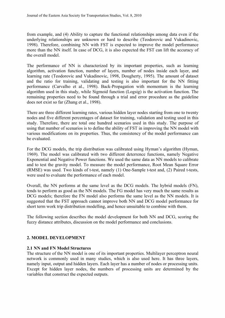
Left Right Left Right Less than 1 1.000 0.034 0.017 About 15 0.483 0.552 0.534 About 1 0.966 0.069 0.052 About 16 0.448 0.586 0.569 About 2 0.931 0.103 0.086 About 17 0.414 0.621 0.603 About 3 0.897 0.138 0.121 About 18 0.379 0.655 0.638 About 4 0.862 0.172 0.155 About 19 0.345 0.690 0.672 About 5 0.828 0.207 0.190 About 20 0.310 0.724 0.707 About 6 0.793 0.241 0.224 About 21 0.276 0.759 0.741 About 7 0.759 0.276 0.259 About 22 0.241 0.793 0.776 About 8 0.724 0.310 0.293 About 23 0.207 0.828 0.810 About 9 0.690 0.345 0.328 About 24 0.172 0.862 0.845 About 10 0.655 0.379 0.362 About 25 0.138 0.897 0.879 About 11 0.621 0.414 0.397 About 26 0.103 0.931 0.914 About 12 0.586 0.448 0.431 About 27 0.069 0.966 0.948 About 13 0.552 0.483 0.466 More than 27 0.034 1.000 0.983 About 14 0.517 0.517 0.500 3. MODEL OUTPUT AND DISCUSSION 3.1 NN and FN Model Performance The behaviours of both NN and FN models are very similar for all variations in the network properties. They behave very much the same (see Tables 3 and 4). For examples are the experiments for validated networks with three different learning rates (0.1, 0.01, and 0.001). The training was stopped at generally almost the same epoch.

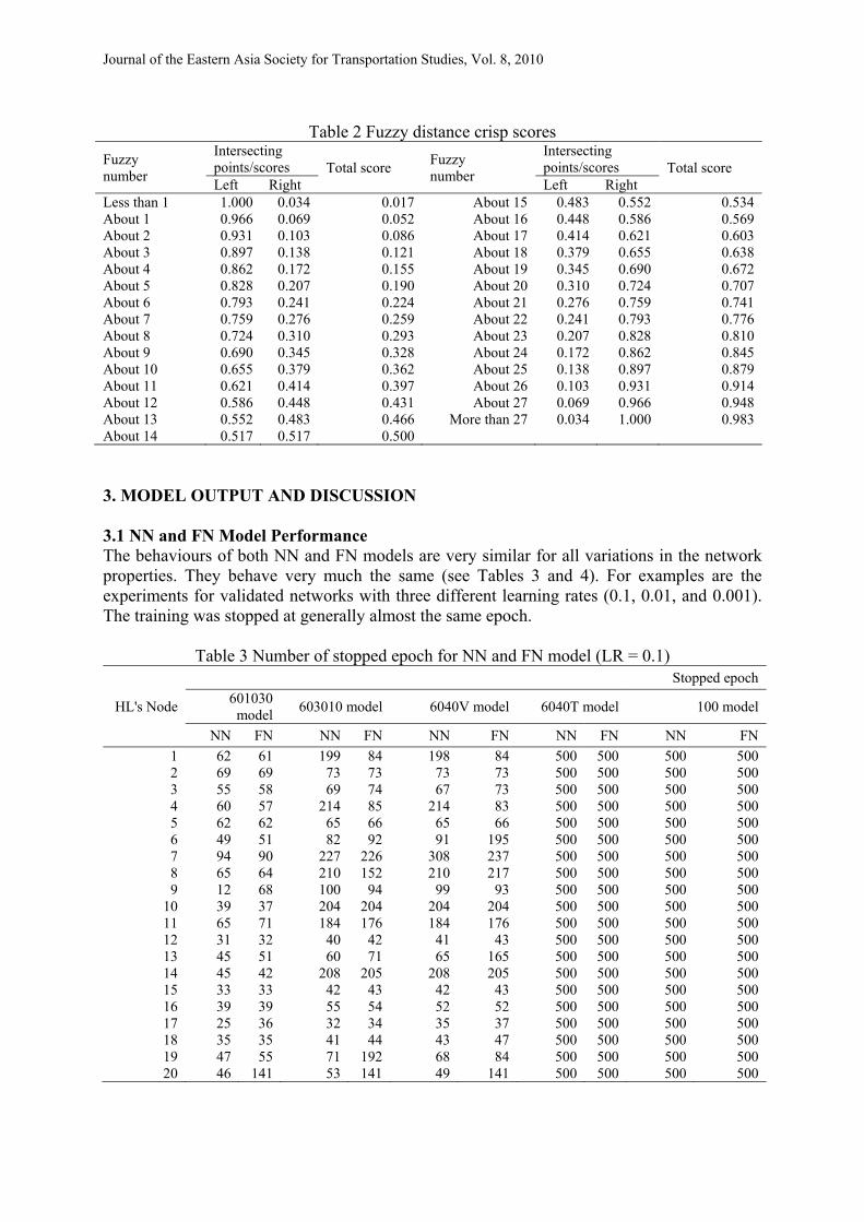
Table 3 Number of stopped epoch for NN and FN model (LR = 0.1)

HL's Node

Stopped epoch 601030

model 603010 model 6040V model 6040T model 100 model

NN FN NN FN NN FN NN FN NN FN 1 62 61 199 84 198 84 500 500 500 500 2 69 69 73 73 73 73 500 500 500 500 3 55 58 69 74 67 73 500 500 500 500 4 60 57 214 85 214 83 500 500 500 500 5 62 62 65 66 65 66 500 500 500 500 6 49 51 82 92 91 195 500 500 500 500 7 94 90 227 226 308 237 500 500 500 500 8 65 64 210 152 210 217 500 500 500 500 9 12 68 100 94 99 93 500 500 500 500

10 39 37 204 204 204 204 500 500 500 500 11 65 71 184 176 184 176 500 500 500 500 12 31 32 40 42 41 43 500 500 500 500 13 45 51 60 71 65 165 500 500 500 500 14 45 42 208 205 208 205 500 500 500 500 15 33 33 42 43 42 43 500 500 500 500 16 39 39 55 54 52 52 500 500 500 500 17 25 36 32 34 35 37 500 500 500 500 18 35 35 41 44 43 47 500 500 500 500 19 47 55 71 192 68 84 500 500 500 500 20 46 141 53 141 49 141 500 500 500 500


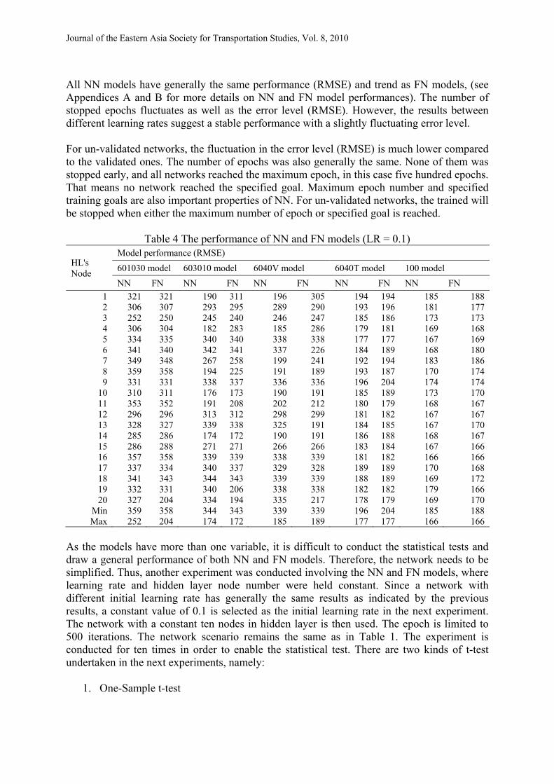
All NN models have generally the same performance (RMSE) and trend as FN models, (see Appendices A and B for more details on NN and FN model performances). The number of stopped epochs fluctuates as well as the error level (RMSE). However, the results between different learning rates suggest a stable performance with a slightly fluctuating error level. For un-validated networks, the fluctuation in the error level (RMSE) is much lower compared to the validated ones. The number of epochs was also generally the same. None of them was stopped early, and all networks reached the maximum epoch, in this case five hundred epochs. That means no network reached the specified goal. Maximum epoch number and specified training goals are also important properties of NN. For un-validated networks, the trained will be stopped when either the maximum number of epoch or specified goal is reached.

Table 4 The performance of NN and FN models (LR = 0.1)

HL's Node

Model performance (RMSE) 601030 model 603010 model 6040V model 6040T model 100 model NN FN NN FN NN FN NN FN NN FN

1 321 321 190 311 196 305 194 194 185 188 2 306 307 293 295 289 290 193 196 181 177 3 252 250 245 240 246 247 185 186 173 173 4 306 304 182 283 185 286 179 181 169 168 5 334 335 340 340 338 338 177 177 167 169 6 341 340 342 341 337 226 184 189 168 180 7 349 348 267 258 199 241 192 194 183 186 8 359 358 194 225 191 189 193 187 170 174 9 331 331 338 337 336 336 196 204 174 174

10 310 311 176 173 190 191 185 189 173 170 11 353 352 191 208 202 212 180 179 168 167 12 296 296 313 312 298 299 181 182 167 167 13 328 327 339 338 325 191 184 185 167 170 14 285 286 174 172 190 191 186 188 168 167 15 286 288 271 271 266 266 183 184 167 166 16 357 358 339 339 338 339 181 182 166 166 17 337 334 340 337 329 328 189 189 170 168 18 341 343 344 343 339 339 188 189 169 172 19 332 331 340 206 338 338 182 182 179 166 20 327 204 334 194 335 217 178 179 169 170

Min 359 358 344 343 339 339 196 204 185 188 Max 252 204 174 172 185 189 177 177 166 166

As the models have more than one variable, it is difficult to conduct the statistical tests and draw a general performance of both NN and FN models. Therefore, the network needs to be simplified. Thus, another experiment was conducted involving the NN and FN models, where learning rate and hidden layer node number were held constant. Since a network with different initial learning rate has generally the same results as indicated by the previous results, a constant value of 0.1 is selected as the initial learning rate in the next experiment. The network with a constant ten nodes in hidden layer is then used. The epoch is limited to 500 iterations. The network scenario remains the same as in Table 1. The experiment is conducted for ten times in order to enable the statistical test. There are two kinds of t-test undertaken in the next experiments, namely:

1. One-Sample t-test


It is used to measure the significant difference of average performance (RMSE) of NN and FN compared to DCG models

2. Paired/Match t-test This test is used to measure the significant difference of average performance (RMSE) between NN and FN models

All tests were conducted by using SPSS Statistic 17.0 software. The results of the experiments and testing are reported later in this paper. 3.2 DCG and FG Model Performance The results of DCG and FG models are reported in Table 5. Both DCG and FG models were calibrated and tested with the same data, except for the trip length. Fuzzy distance was used to calibrate the FG model. The fuzzy distance was converted to crisp score before being used. Both models were calibrated by using Hyman’s algorithm, known as a robust maximum likelihood method for calibration. The calibration parameter value (β) for DCG and FG is significantly different, obtained after eight times of iteration where the difference between observed and modelled trip length equals to 0. Despite a great difference in the calibration parameter (β) value, both DCG and FG models perform relatively the same. They both have almost the same RMSE, which is 167 (Table 5). Compared to negative exponential function, the gravity model performance with deterrence function of negative power has a 23 per cent higher RMSE. It also has a higher RMSE than FG model with the same deterrence function, by 2 per cent.

Table 5 DCG and FG calibration parameter and RMSE Deterrence function Calibration parameter (β) RMSE

DCG FG DCG FG Negative Exponential 0.109 3.199 167 167 Negative Power 0.539 0.649 206 202

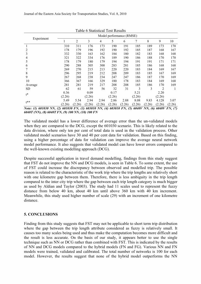
3.3 Statistical Test Results The results of the modified NN and FN models as explained in section 3.1 are reported in Table 6. It also shows the t-test outcomes for all scenarios and models. The first test (t*) is Paired/Match t-test between NN and FN models, while the second one (t**) is One-Sample t-tests of NN and FN compared to DCG models. All tests are based on two-tail t-tests with level of confident 95 per cent. The paired test results between NN and FN models suggest that the average performance is statistically the same, except for the 6040T model. The average RMSE for this scenario is statistically different, where the NN model has a lower error than the FN. However, this model is un-validated one, therefore, the result cannot be generalized. Another un-validated model (100 Model) has a calculated value of t which almost reaches the critical value (t-table value =2.26). For this scenario, FN model has a lower error than NN model which is contrast to previous model.


Table 6 Statistical Test Results

Experiment Model performance (RMSE)

1 2 3 4 5 6 7 8 9 10 1 310 311 176 173 190 191 185 189 173 170 2 178 179 196 192 190 192 185 187 168 167 3 332 330 163 162 184 180 182 183 168 168 4 321 322 334 176 189 190 186 188 170 170 5 178 179 180 179 194 194 191 191 171 171 6 290 288 305 300 283 281 185 186 168 168 7 269 270 215 213 220 220 183 184 169 167 8 296 295 219 212 208 209 183 185 167 169 9 267 268 238 234 247 247 186 187 170 169 10 366 367 166 329 180 178 183 184 169 168 Average 281 281 219 217 208 208 185 186 170 169 SD 62 61 59 56 32 31 3 3 2 1

t* 0.36 (2.26) 0.09

(2.26) 0.17 (2.26) 5.21

(2.26) 2.20 (2.26)

t** 5.49 (2.26)

5.54 (2.26)

2.94 (2.26)

2.94 (2.26)

2.86 (2.26)

2.88 (2.26)

8.08 (2.26)

9.83 (2.26)

4.128 (2.26)

3.07 (2.26)

Note: (1) 601030 NN, (2) 601030 FN, (3) 603010 NN, (4) 603010 FN, (5) 6040V NN, (6) 6040V FN, (7) 6040T (NN), (8) 6040T FN, (9) 100 NN, (10) 100 FN The validated model has a lower difference of average error than the un-validated models when they are compared to the DCG, except the 601030 scenario. This is likely related to the data division, where only ten per cent of total data is used in the validation process. Other validated model scenarios have 30 and 40 per cent data for validation. Based on this finding, using a higher percentage of data for validation can improve the average neural network model performance. It also suggests that validated model can have lower errors compared to the well-known existing modelling approach (DCG). Despite successful application in travel demand modelling, findings from this study suggest that FST do not improve the NN and DCG models, is seen in Table 6. To some extent, the use of FST could increase the discrepancy between observed and modelled trip. The possible reason is related to the characteristic of the work trip where the trip lengths are relatively short with one kilometre gap between them. Therefore, there is less ambiguity in the trip length compared to the inter city trip where the gap between each trip length category is much bigger as used by Aldian and Taylor (2003). The study had 11 scales used to represent the fuzzy distance from below 40 km, about 40 km until above 360 km with 40 km increment. Meanwhile, this study used higher number of scale (29) with an increment of one kilometre distance. 5. CONCLUSIONS Finding from this study suggests that FST may not be applicable to short term trip distribution where the gap between the trip length attribute considered as fuzzy is relatively small. It causes too many scales being used and thus make the computation becomes more difficult and the result is less accurate. On the basis of our study, it appears better to use the single technique such as NN or DCG rather than combined with FST. This is indicated by the results of NN and DCG models compared to the hybrid models (FN and FG). Various NN and FN models were trained, validated and calibrated. The total number of networks is 100 for each model. However, the results suggest that none of the hybrid model outperforms the NN


models. The performance of FG models is about the same as DCG ones. It can be concluded that FST may be unsuitable to be used in modelling short distance trip such as work trip as indicated by this study.

REFERENCES ALDIAN, A. (2003) Analysis of Travel Demand in Developing Countries: A fuzzy Multiple Attribute

Decision‐Making Approach. 26th Australasian Transport Research Forum. Wellington, New Zealand, ATRF.

ALDIAN, A. & TAYLOR, M. A. P. (2003) Fuzzy multicriteria analysis for inter‐city travel demand modelling. Journal of the Eastern Asia Society for Transportation Studies, 5, 1294‐1307.

BLACK, W. R. (1995) Spatial interaction modeling using artificial neural networks. Journal of Transport Geography, 3, 159‐166.

CANTARELLA, G. E. & DE LUCA, S. (2005) Multilayer feedforward networks for transportation mode choice analysis: An analysis and a comparison with random utility models. Transportation Research Part C: Emerging Technologies, 13, 121‐155.

CARVALHO, M. C. M., DOUGHERTY, M. S., FOWKES, A. S. & WARDMAN, M. R. (1998) Forecasting travel demand: a comparison of logit and artificial neural network methods. The Journal of the Operational Research Society, 49, 711‐722.

CHEN, S. J. & HWANG, C. L. (1992) Fuzzy Multiple Attribute Decision Making. Lectures Notes in Economics and Mathematical Systems, Pringer‐Verlag.

DELL'ORCO, M., CIRCELLA, G. & SASSANELLI, D. (2007) A hybrid approach to combine fuzziness and randomness in travel choice prediction. European Journal of Operational Research, 185, 648‐658.

DOUGHERTY, M. (1995) A review of neural networks applied to transport. Transportation Research Part C: Emerging Technologies, 3, 247‐260.

HENSHER, D. A. & BUTTON, K. J. (2000) Introduction. IN HENSHER, D. A. & BUTTON, K. J. (Eds.) Handbook of Transport Modelling. Oxford, UK, Elsevier Science Ltd.

HENSHER, D. A. & TON, T. T. (2000) A comparison of the predictive potential of artificial neural networks and nested logit models for commuter mode choice. Transportation Research Part E: Logistics and Transportation Review, 36, 155‐172.

HWANG, C. L. & YOON, K. (1979) Multiple Attribute Decision Making: Methods and Applications, Berlin, Springer‐Verlag.

HYMAN, G. M. (1969) The Calibration of Trip Distribution Models. Environment and Planning, 1, 105‐112.

MOZOLIN, M., THILL, J. C. & LYNN, U. E. (2000) Trip distribution forecasting with multilayer perceptron neural networks: A critical evaluation. Transportation Research Part B: Methodological, 34, 53‐73.

SUBBA RAO, P. V., SIKDAR, P. K., KRISHNA RAO, K. V. & DHINGRA, S. L. (1998) Another insight into artificial neural networks through behavioural analysis of access mode choice. Computers, Environment and Urban Systems, 22, 485‐496.

TEODOROVIC, D. & VUKADINOVIC, K. (1998) Traffic Control and Transport Planning: A Fuzzy Sets and Neural Networks Approach, Massachusetts, USA, Kluwer Academic Publisher.

YIN, H., WONG, S. C., XU, J. & WONG, C. K. (2002) Urban traffic flow prediction using a fuzzy‐neural approach. Transportation Research Part C: Emerging Technologies, 10, 85‐98.

ZADEH, L. A. (1965) Fuzzy Sets. Information and control, 8, 338‐353. ZHANG, G., PATUWO, B. E. & HU, M. Y. (1998) Forecasting with artificial neural networks:: The state

of the art. International Journal of Forecasting, 14, 35‐62. ZIMMERMANN, H. J. (1991) Fuzzy Set Theory and Its applications, Massachusetts, Kluwer Academic

Publisher.


Appendix A The performance of NN and FN models (LR = 0.01)

HL's Node

Model performance (RMSE) 601030 model 603010 model 6040V model 6040T model 100 model NN FN NN FN NN FN NN FN NN FN

1 322 321 190 311 196 305 195 195 185 189 2 301 313 293 295 289 290 194 195 182 180 3 254 253 244 239 246 246 183 189 177 181 4 305 305 171 283 180 286 186 182 170 168 5 334 335 340 340 338 338 176 177 167 169 6 342 341 342 341 337 337 187 189 169 182 7 348 348 269 255 255 201 195 195 185 187 8 359 358 192 223 190 193 194 186 171 175 9 331 331 338 337 336 336 196 198 175 176

10 308 308 180 176 192 193 187 189 174 171 11 353 352 180 165 195 179 178 176 168 168 12 293 294 178 178 183 185 181 183 170 168 13 327 327 338 338 325 324 184 184 167 170 14 285 286 183 182 194 195 185 186 169 168 15 288 288 270 270 265 265 184 185 167 170 16 362 361 180 164 179 180 180 183 169 166 17 336 336 339 336 328 327 185 189 170 169 18 342 342 343 342 339 193 187 190 170 173 19 332 331 340 339 338 338 182 182 169 167 20 326 205 333 196 334 218 178 179 169 171

Min 362 361 343 342 339 338 196 198 185 189 Max 254 205 171 164 179 179 176 176 167 166

Appendix B The performance of NN and FN models (LR = 0.001)

HL's Node

Model performance (RMSE) 601030 model 603010 model 6040T model 6040V model 100 model NN FN NN FN NN FN NN FN NN FN

1 322 322 191 311 194 196 196 305 185 189 2 302 302 293 295 196 195 289 290 184 184 3 254 251 244 239 185 187 246 246 174 175 4 305 305 170 283 181 182 180 286 171 170 5 334 334 340 340 175 177 338 338 167 169 6 342 340 342 341 189 187 337 337 173 184 7 349 348 204 248 196 199 201 234 189 192 8 358 357 191 223 194 191 190 193 172 175 9 331 331 338 337 200 198 336 336 176 184

10 309 309 174 179 188 191 188 289 174 172 11 353 352 162 208 177 178 176 210 168 168 12 294 293 180 180 181 183 184 186 168 167 13 327 327 338 338 184 186 324 324 167 170 14 285 286 183 182 186 191 194 195 173 172 15 286 286 270 270 182 184 265 265 167 166 16 362 361 180 166 180 181 181 182 167 367 17 337 335 339 336 186 196 328 327 172 170 18 342 342 343 342 186 186 339 194 170 197 19 332 331 340 339 182 183 338 338 169 168 20 326 205 333 194 183 185 334 218 187 215

Min 362 361 343 342 200 199 339 338 189 367 Max 254 205 162 166 175 177 176 182 167 166

Documents

Examining the Possibility of Fuzzy Set Theory Application in