Embed Size (px)
Citation preview

Examining Model Predictions of Zinc and Copper Aqueous Speciation and Freshwater Ecotoxicity: Case Study of
Ross Lake, Flin Flon, Manitoba, Canada
by
Sumera Yacoob
A thesis submitted in conformity with the requirements for the degree of Master of Applied Science
Department of Chemical Engineering and Applied Chemistry University of Toronto
© Copyright by Sumera Yacoob 2013
ii
Examining Model Predictions of Zinc and Copper Aqueous Speciation and Freshwater Ecotoxicity: Case Study at
Ross Lake, Flin Flon, Manitoba, Canada
Sumera Yacoob
Master of Applied Science
Department of Chemical Engineering and Applied Chemistry
University of Toronto
2013
Abstract
Models of aqueous metal speciation and ecotoxicity have become commonplace due to their
ability to estimate metal behaviour. This study evaluated commonly used aqueous geochemical
speciation and ecotoxicity models with application to a mine impacted lake in northern
Manitoba.
The geochemical speciation model Winderemere Humic Aqueous Model (WHAM) was
compared with Diffusive Gradients in Thinfilm (DGT) measurements of zinc and copper. DGT
measurements in the water column corresponded well with WHAM-estimated Zn2+
, Cu2+
was off
by up to 100x. Additional metal, either from small organic bound species or dissolution of metal
sulphides from resuspended sediment, served to improve model estimates.
The single metal Biotic Ligand Model (BLM) predicted acute toxicity to Daphnia magna
attributable to copper but not zinc, at low pH (3.55 – 5.5). Comparison of results did not show a
significant difference between the single and mixture BLMs, suggesting a non-interactive effect
on metal toxicity for measured water chemistry.

iii
Acknowledgements
I would like to express my heartfelt thanks to Professor Miriam Diamond for her support,
patience and hard work throughout this process, without which this project may never have been
completed. This project presented many challenges along the way, and her understanding and
positivity were essential to this coming together.
I would like to thank HBMS for funding this project. In particular I would like to thank Stephen
West, Joel Nielson and Ray Tardiff for their kindness and help during my trips to Flin Flon.
Thank you to Robert Santore and Dr. Helga Sonnenberg for your expertise and helpful
discussions which always reinvigorated my interest in this topic.
Thank you to Dr. Celine Gueguen for all her helpful contributions on the project and
participation on my defense committee.
I thank Professors Charles Jia and Susan Andrews for participating in my defense committee.
Appreciation and thanks go out to the entire Diamond Lab group. Your smiling faces and
suggestions and advice were always helpful. In particular, thank you to Dr. Emma Goosey for all
your help in the field and lab.
Thank you to all of my family and friends, who supported my work and never let me be too hard
on myself. Thanks especially go out to my parents and sister whose pride in my work always
touched my heart and for supporting my decision to leave consulting and focus on academia.
And lastly, but certainly never least, thank you to my husband Imran whose love, patience,
generosity, advice, listening ear and computer programming skills helped more than you realize.

iv
Table of Contents
Acknowledgements ........................................................................................................................ iii
List of Tables ................................................................................................................................ vii
List of Figures .............................................................................................................................. viii
List of Appendices ......................................................................................................................... ix
Chapter 1 Introduction .....................................................................................................................1
1.1 Study Metals and Study Site ................................................................................................2
1.1.1 Zinc ..........................................................................................................................2
1.1.2 Copper ......................................................................................................................3
1.2 Geochemical and Ecotoxicity Modelling .............................................................................3
1.3 Diffusive Gradient Thinfilms ...............................................................................................5
1.4 Project Summary ..................................................................................................................6
1.5 Research Objectives .............................................................................................................6
1.6 Thesis Outline (Outline all papers contained) .....................................................................6
1.7 References ............................................................................................................................8
Chapter 2 - Comparing DGT Measurements and WHAM Estimates of Zinc and Copper: A
Case Study at Ross Lake in Northern Canada ..........................................................................10
2 Abstract .....................................................................................................................................10
2.1 Introduction ........................................................................................................................11
2.2 Case Study .........................................................................................................................14
2.3 Field Measurements ...........................................................................................................15
2.3.1 DGT Deployment...................................................................................................15
2.3.2 DGT Analysis ........................................................................................................16
2.4 Water Chemistry Sampling ................................................................................................17
2.5 Geochemical Modeling ......................................................................................................17

v
2.6 Comparison of DGT to WHAM Predicted Free Ion Concentration ..................................18
2.7 Comparing DGT Values to Metal Bound to DOC.............................................................20
2.8 Dissolution Kinetics ...........................................................................................................21
2.9 Implications........................................................................................................................23
2.10 Tables .................................................................................................................................25
2.11 Figures................................................................................................................................28
2.12 References ..........................................................................................................................32
Chapter 3 - Investigating Toxicity Using Single and Metal Mixture BLM Models: A Case
Study at Ross Lake ....................................................................................................................35
3 Abstract .....................................................................................................................................35
3.1 Introduction ........................................................................................................................36
3.2 Case Study – Ross Lake .....................................................................................................37
3.3 Methods..............................................................................................................................39
3.3.1 Field Measurements ...............................................................................................39
3.3.2 Speciation and Toxicity Modelling Using WHAM and BLM ...............................40
3.4 Results ................................................................................................................................41
3.4.1 Measured Water Chemistry ...................................................................................41
3.4.2 Metal Speciation and Toxicity ...............................................................................42
3.4.3 Single Versus Metal Mixture BLM Toxicity Analysis ..........................................43
3.5 Implications........................................................................................................................45
3.6 Tables .................................................................................................................................47
3.7 References ..........................................................................................................................51
Chapter 4 - Conclusions .................................................................................................................54
4 Research Summary....................................................................................................................54
4.1 Scientific Contributions .....................................................................................................55

vi
4.2 Research Outlook ...............................................................................................................56
4.3 References ..........................................................................................................................57
vii
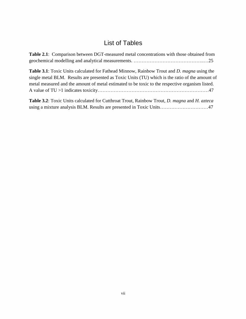
List of Tables
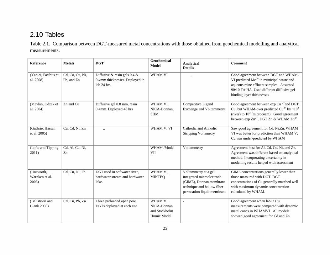
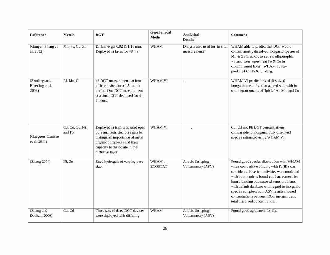
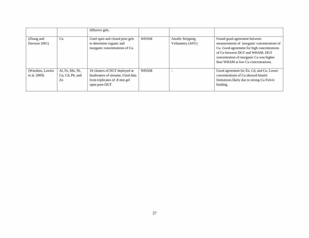
Table 2.1: Comparison between DGT-measured metal concentrations with those obtained from
geochemical modelling and analytical measurements. ……………………………………..…25
Table 3.1: Toxic Units calculated for Fathead Minnow, Rainbow Trout and D. magna using the
single metal BLM. Results are presented as Toxic Units (TU) which is the ratio of the amount of
metal measured and the amount of metal estimated to be toxic to the respective organism listed.
A value of TU >1 indicates toxicity……………………………………………………………47
Table 3.2: Toxic Units calculated for Cutthroat Trout, Rainbow Trout, D. magna and H. azteca
using a mixture analysis BLM. Results are presented in Toxic Units…………………………47
viii
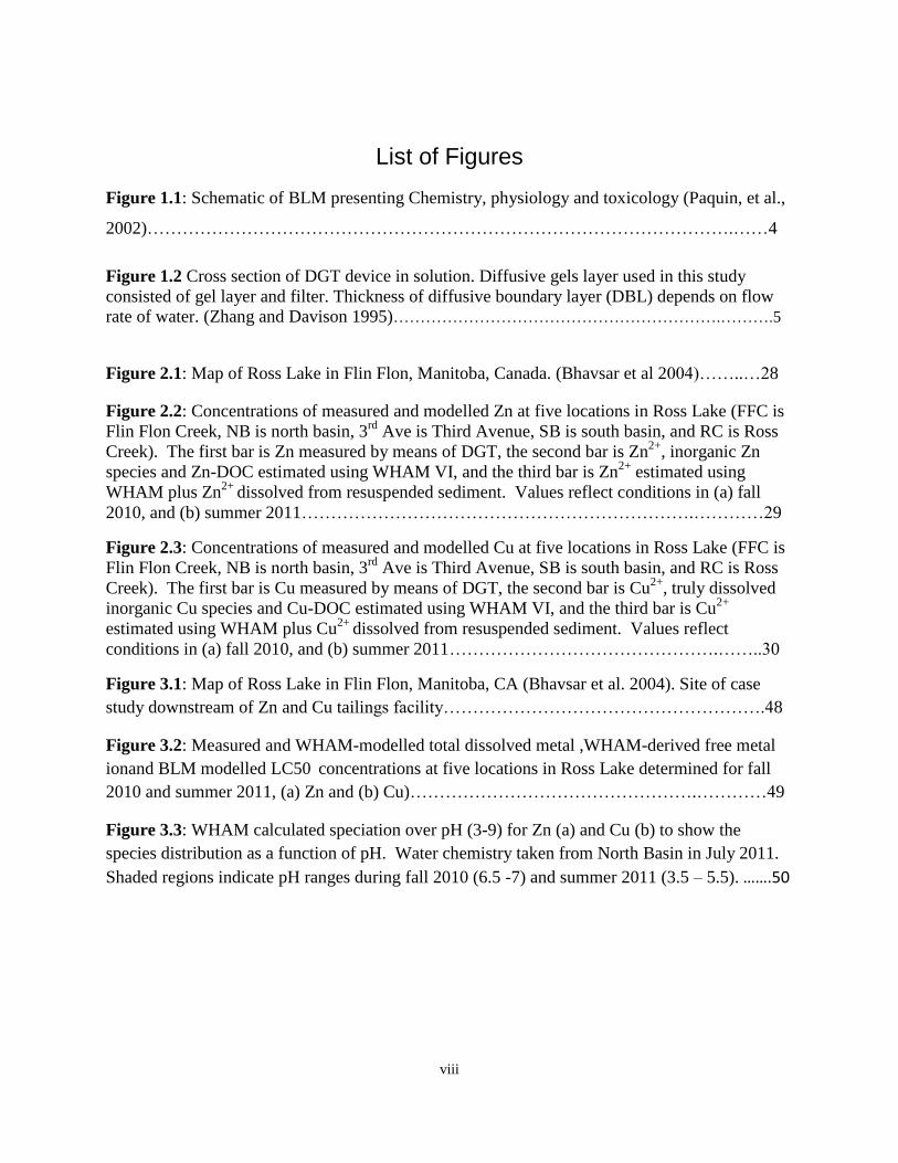
List of Figures
Figure 1.1: Schematic of BLM presenting Chemistry, physiology and toxicology (Paquin, et al.,
2002)……………………………………………………………………………………….……4
Figure 1.2 Cross section of DGT device in solution. Diffusive gels layer used in this study
consisted of gel layer and filter. Thickness of diffusive boundary layer (DBL) depends on flow
rate of water. (Zhang and Davison 1995)…………………………………………………….……….5
Figure 2.1: Map of Ross Lake in Flin Flon, Manitoba, Canada. (Bhavsar et al 2004)……..…28
Figure 2.2: Concentrations of measured and modelled Zn at five locations in Ross Lake (FFC is
Flin Flon Creek, NB is north basin, 3rd
Ave is Third Avenue, SB is south basin, and RC is Ross
Creek). The first bar is Zn measured by means of DGT, the second bar is Zn2+
, inorganic Zn
species and Zn-DOC estimated using WHAM VI, and the third bar is Zn2+
estimated using
WHAM plus Zn2+
dissolved from resuspended sediment. Values reflect conditions in (a) fall
2010, and (b) summer 2011………………………………………………………….…………29
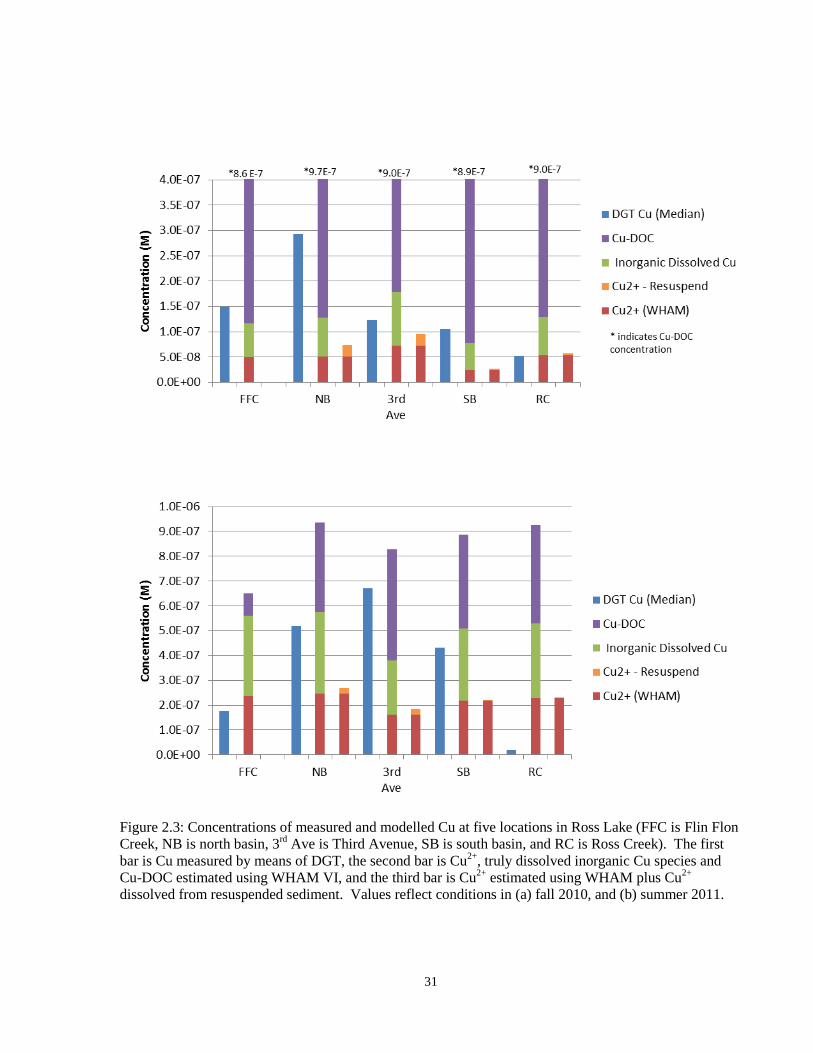
Figure 2.3: Concentrations of measured and modelled Cu at five locations in Ross Lake (FFC is
Flin Flon Creek, NB is north basin, 3rd
Ave is Third Avenue, SB is south basin, and RC is Ross
Creek). The first bar is Cu measured by means of DGT, the second bar is Cu2+
, truly dissolved
inorganic Cu species and Cu-DOC estimated using WHAM VI, and the third bar is Cu2+
estimated using WHAM plus Cu2+
dissolved from resuspended sediment. Values reflect
conditions in (a) fall 2010, and (b) summer 2011……………………………………….……..30
Figure 3.1: Map of Ross Lake in Flin Flon, Manitoba, CA (Bhavsar et al. 2004). Site of case
study downstream of Zn and Cu tailings facility……………………………………………….48
Figure 3.2: Measured and WHAM-modelled total dissolved metal ,WHAM-derived free metal
ionand BLM modelled LC50 concentrations at five locations in Ross Lake determined for fall
2010 and summer 2011, (a) Zn and (b) Cu)………………………………………….…………49
Figure 3.3: WHAM calculated speciation over pH (3-9) for Zn (a) and Cu (b) to show the
species distribution as a function of pH. Water chemistry taken from North Basin in July 2011.
Shaded regions indicate pH ranges during fall 2010 (6.5 -7) and summer 2011 (3.5 – 5.5). …….50

ix
List of Appendices
Appendix 1: Supporting Information for Chapter 2…………………………………………58
Appendix 2: Supporting Information for Chapter 3…………………………………………63
Appendix 3: Detailed Report on Analytical Methods, Results and Quality Control ……......67

1
Chapter 1 Introduction
1. Introduction
Metals are used for numerous purposes in our daily lives. As such, mining and mineral
processing is a large industry, particularly in Canada which is rich in mineral resources.
Unfortunately, as a result of increased metal production, discharges from some mining sites have
led to environmental contamination at concentrations toxic to biota (Taylor et al, 2010).
The study of metals in the environment is complicated due to their ability to exist as different
chemical species. Total and dissolved metal concentrations are often the criteria through which
metal contamination is assessed. These concentrations, however, only give a limited idea of the
nature and toxicity of metals in the environment. Metals speciate differently dependant on
ambient water chemistry, rendering similar dissolved concentrations of metals toxic in some
lakes and non-toxic in others.
Measurement techniques for metal speciation and toxicity can be costly, timely and impractical;
therefore the use of mathematical models is becoming increasingly commonplace. Mathematical
models allow for the prediction of metal species distribution and toxicity based on water
chemistry parameters which are easily obtained.
Mathematical models are constantly evolving with the state of the science and must be evaluated
in order to ensure we have an accurate understanding of environmental conditions. All models
are based on simplifying assumptions that may not always be appropriate. As our understanding
of metal chemistry evolves, so to must the models.
With the improvement of geochemical speciation and toxicity models, we may at some point be
able to set site-specific water quality criteria with the intention of improving water quality
standards. By doing this we can consider ambient water quality and its impact on metal
speciation in setting regulatory limits on metal concentrations.
Data collected from Ross Lake in Flin Flon, Manitoba has been used as a case study for this
thesis research. Ross Lake has a history of high metal concentrations as it is directly

2
downstream of a mine tailings facility that has been operated by Hudson Bay Mining and
Smelting (HBMS) in the town of Flin Flon for over 80 years.
1.1 Study Metals and Study Site
Metal speciation and toxicity measurements and modelling were performed on zinc (Zn) and
copper (Cu). Zn and Cu have been mined by HBMS at their Flin Flon site since the 1930s and
Ross Lake has been subjected to extremely large inputs of metals as a result. As such Ross Lake
has high contamination of these metals. In particular, high Zn concentrations have become a
concern, as Ross Lake has been converted from a net sink for Zn to a net source (Bhavsar et al.
2004a,b). Cu concentrations in the lake have generally been below levels specified by
government regulations, and have not been cause for concern.
1.1.1 Zinc
Over 11 million tons of Zn is produced on an annual basis globally, most of it for galvanizing to
protect steel from corrosion (International Zinc Association, 2011). Other uses include
production of brass, bronze and other Zn alloys (USGS, 2013). Zn is used by a variety of
industries such as transportation, construction, consumer goods and general engineering
(International Zinc Association, 2011)
Zn is an essential mineral for all organisms, necessary for functions such as cellular metabolism,
protein synthesis, wound healing and DNA synthesis. Zn also promotes healthy growth in
pregnancy, childhood and adolescence in humans (National Institutes of Health, 2011).
Zn occurs naturally in air, water and soil (International Zinc Association, 2011), however due to
anthropogenic inputs, background concentrations are rising. Industrial discharges from mining,
coal and waste combustion and steel processing all contribute to higher Zn concentrations in the
environment (Agency for Toxic Substances and Disease Registry , 2013). These industrial
discharges into air, soil and water then result in environmental exposures.
At elevated levels Zn can cause toxicity to animals and is phytotoxic (Manahan, 2001). The free
ion form of Zn is toxic to aquatic life in the micromolar range (Muyssen et al. 2006). However

3
the toxicity of Zn is highly dependent on water chemistry parameters such as pH and hardness
(Heijerick et al. 2002)
1.1.2 Copper
Cu is one of the oldest metals in use because of its properties of ductility, malleability, thermal
and electrical conductivity and resistance to corrosion (USGS 2013). Cu is a commonly found
trace element in the earths crust (Flemming & Trevors, 1989). Cu is used in building
construction, electronics, transportation, industrial machinery and general products (USGS,
2013). Electrical uses account for 75% of Cu use. Cu can enter the environment through
smelting, mining, industrial and domestic waste emission, application of fertilizers, sewage
sludge, algicides, fungicides and molluscicides (Flemming & Trevors, 1989).Cu is an essential
element for humans and animals however high concentrations are toxic resulting in damage to
liver and sometimes kidneys (Stern 2010). Due to the high toxicity that Cu poses to algea,
copper sulphate has commonly been used as an algicide in eutrophic lakes (Flemming &
Trevors, 1989).
Cu has a strong affinity for binding with organic ligands in solution and for that reason is
typically not bioavailable (Arai, Harino et al. 2009). As with Zn, Cu in its free ion form is most
toxic, as well as CuOH+ (de Schamphelaere and Janssen 2001). Again, its toxicity is very
sensitive to pH and water chemistry.
1.2 Geochemical and Ecotoxicity Modelling
Geochemical speciation models are based on the simplifying assumption of thermodynamic
equilibrium. Although several geochemical models are commercially available, this study makes
use of the Windermere Humic Aqueous Model (WHAM) (Tipping, 1994) to be consistent with
toxicity calculations done using the Biotic Ligand Model (BLM).
WHAM is advanced in its ability to account for organic matter in both the colloidal and
particulate phase (Gandhi et al. 2011).The model makes use of a variety of submodels such as
the Humic Ion Binding Model V, an inorganic speciation code for aqueous solution, precipitation
of aluminum and iron oxyhydroxides, cation-exchange on representative clay and the adsorption-
desorption of fulvic acids (Tipping, 1994). WHAM uses as input, a number of easily obtained

4
water chemistry parameters (e.g., pH, DOC, cation concentrations, anion concentrations) to
calculate speciation. All of our calculations have made use of the WHAM default data base of
stability constants.
BLM was used to predict metal toxicity to aquatic species using Ross Lake as a case study. The
BLM uses site specific water quality to determine LC50 values (Paquin, et al., 2002). BLM is an
extension of geochemical modelling with the addition of the gill as a biotic ligand with a
particular metal binding strength (Playle, 2004). A downloadable version of BLM is made
available through HydroQual®. The model pairs physiology and water chemistry to determine
toxicity (Figure 1).
Figure 1.1 - Schematic of BLM presenting chemistry, physiology and toxicology (Paquin, et al.,
2002)
The BLM takes into consideration competitive effects from cations and complexation of anionic
species which may inhibit toxicity (Playle, 2004). Current versions of BLM consider a single
metal. Santore et al. (in prep) have developed a new version that considers the competitive
effects of metal mixtures at the biotic ligand.
5
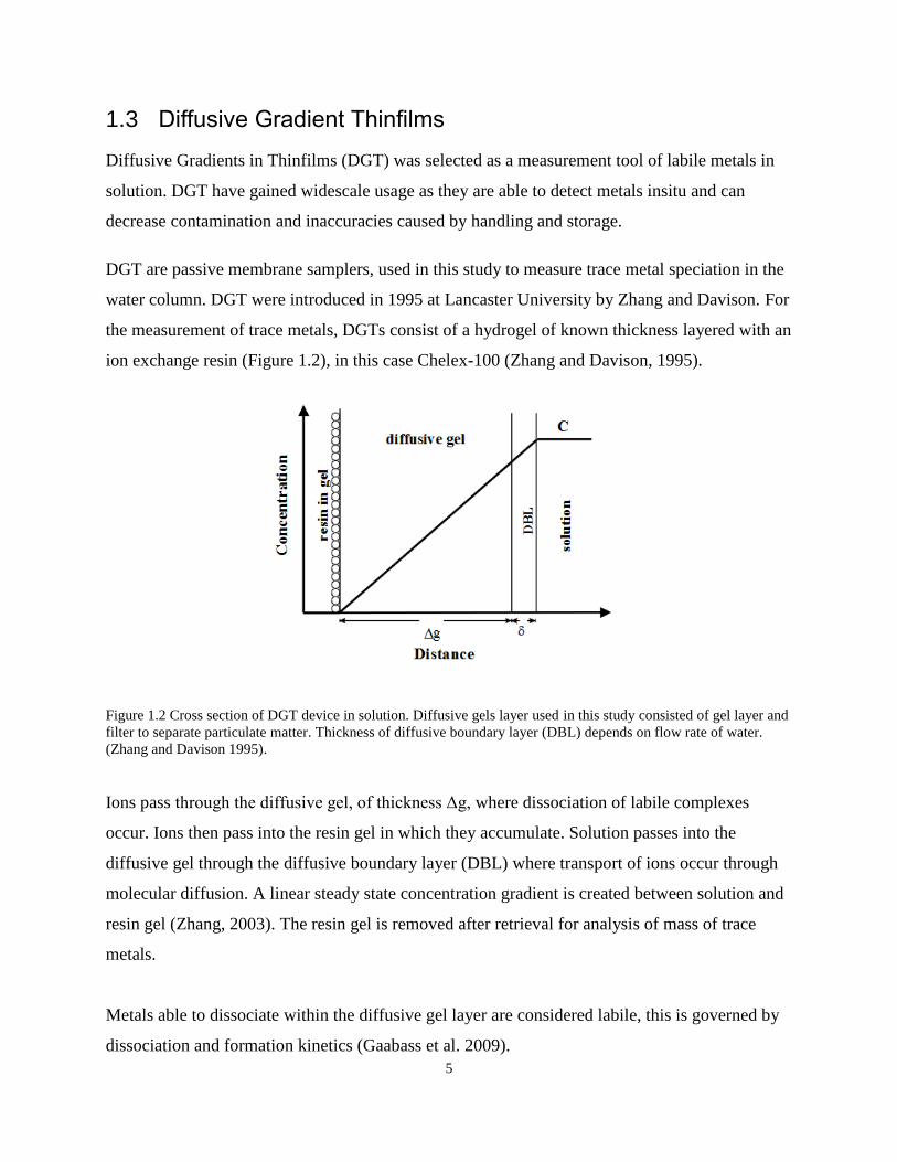
1.3 Diffusive Gradient Thinfilms
Diffusive Gradients in Thinfilms (DGT) was selected as a measurement tool of labile metals in
solution. DGT have gained widescale usage as they are able to detect metals insitu and can
decrease contamination and inaccuracies caused by handling and storage.
DGT are passive membrane samplers, used in this study to measure trace metal speciation in the
water column. DGT were introduced in 1995 at Lancaster University by Zhang and Davison. For
the measurement of trace metals, DGTs consist of a hydrogel of known thickness layered with an
ion exchange resin (Figure 1.2), in this case Chelex-100 (Zhang and Davison, 1995).
Figure 1.2 Cross section of DGT device in solution. Diffusive gels layer used in this study consisted of gel layer and
filter to separate particulate matter. Thickness of diffusive boundary layer (DBL) depends on flow rate of water.
(Zhang and Davison 1995).
Ions pass through the diffusive gel, of thickness Δg, where dissociation of labile complexes
occur. Ions then pass into the resin gel in which they accumulate. Solution passes into the
diffusive gel through the diffusive boundary layer (DBL) where transport of ions occur through
molecular diffusion. A linear steady state concentration gradient is created between solution and
resin gel (Zhang, 2003). The resin gel is removed after retrieval for analysis of mass of trace
metals.
Metals able to dissociate within the diffusive gel layer are considered labile, this is governed by
dissociation and formation kinetics (Gaabass et al. 2009).

6
The labile metal concentration (Cdgt) is calculated using the following equation (Zhang and
Davison 1995).
Cdgt= mΔg/DAt (1)
Where m is the mass on the resin gel, Δ g is the thickness of the diffusion gel, D is the diffusivity
of metal ions through the gel, A is the surface area of the gel, and t is the total time deployed
1.4 Project Summary
The goal of my thesis research was to examine speciation and toxicity modeling. In the case of
the geochemical speciation model, model results were compared against field measurements
using several measurement methods. I compared two versions of the Biotic Ligand Model, one
that considers a single metal and the other, a newly developed version that assesses metal
mixtures. Ross Lake was used as a case study for these assessments. As mentioned above, the
lake has elevated levels of Zn and Cu from mining operations. This research has used, as its
basis, previous research conducted on this lake that investigated the speciation, fate and
ecotoxicity of Zn and Cu (Bhavsar et al. 2004 a,b, Gandhi et al. 2011)
1.5 Research Objectives
The following research objectives were addressed in this thesis using Ross Lake, Manitoba, as a
case study:
Conduct field campaign to assess water chemistry,
Model metal speciation and ecotoxicity in water column,
Address discrepancies in speciation estimations through metal dissolution from sediment
and through different interpretations of measured concentrations, and
Determine the metal causing ecotoxicity in Ross Lake
1.6 Thesis Outline (Outline all papers contained)
The chapters of this thesis consist of journal articles in preparation for submission.
Chapter 2 : Comparing DGT Measurements and WHAM Estimates of Zinc and Copper : A Case
Study at Ross Lake in Northern Canada

7
Co-authors: Miriam L. Diamond, Celine Gueguen
Contribution: S. Yacoob performed field work with assistance from Hudson Bay Mining &
Smelting, produced model data, data analysis and wrote manuscript. Reasearch and manuscript
preparation were completed under supervision of M.L. Diamond. C. Gueguen performed
analysis of DGT samples and commented on the manuscript.
This chapter looks at estimations of Zn and Cu speciation using the Windermere Humic
Aqueous Model (WHAM) and evaluates the results against measured concentrations obtained
from Diffusive Gradients in Thinflim (DGT). A summary of similar studies which have
compared model and measurement methods are presented and assessed. The study explores
different reasons for discrepancies between modelled and measured concentrations, both looking
at the shortcomings of measurement technique and model assumptions. This paper also addresses
the vagueness in terminology commonly used in this field of study.
Chapter 3: Investigating Toxicity Using Single and Mixture BLM Models: A Case Study at Ross
Lake
Co-authors: Miriam L. Diamond (University of Toronto), Robert Santore (HydroQual), Helga
Sonnenberg (Stantec Consulting)
Contributions: S. Yacoob performed field work with assistance from Hudson Bay Mining and
Smelting, produced model data for the single metal BLM, analyzed model results and wrote the
manuscript. Research and manuscript preparation were completed under supervision of M.L.
Diamond. Robert Santore provided model results from the metal mixture BLM. Helga
Sonnenberg provided toxicity testing data.
This chapter compares estimates of ecotoxicity from the single metal BLM and the newly
developed metal mixture BLM. Similarities and differences in model results are highlighted and
explained. Efforts are made to explain why acute toxicity is exhibited in specific instances and
not in others.
8
Chapter 4: Conclusions
This chapter contains a summary of findings, scientific contributions and outlook for further
research.
1.7 References
Agency for Toxic Substances and Disease Registry. (2013, March 6). Toxicological Profile for
Zinc. Retrieved March 6, 2013, from Agency for Toxic Substances and Disease Registry Website
: http://www.atsdr.cdc.gov/toxprofiles/tp60-c6.pdf
Arai, T., Harino, H., Ohji, M., & Langston, W. (2009). Ecotoxicology of Antifouling Biocides.
Tokyo: Springer.
Bhavsar, S. P., M. L. Diamond, et al. (2004)a. "Dynamic coupled metal transport-speciation
model: Application to assess a zinc-contaminated lake." Environmental Toxicology and
Chemistry 23(10): 2410-2420.
Bhavsar, S. P., M. L. Diamond, et al. (2004)b. "Development of a coupled metal speciation-fate
model for surface aquatic systems." Environmental Toxicology and Chemistry 23(6): 1376-1385.
de Schamphelaere, K. A. C. and C. R. Janssen (2001). A Biotic Ligand Model Predicting Acute
Copper Toxicity for Daphnia magna: The Effects of Calcium, Magnesium, Sodium, Potassium,
and pH. Environmental Science & Technology , 48-54.
Flemming, C. A., & Trevors, J. (1989). Copper Toxicity and Chemistry in the Environment: A
Review . Water, air, and soil pollution , 143-158.
Gaabass, I., J. D. Murimboh, et al. (2009). "A Study of Diffusive Gradients in Thin Films for the
Chemical Speciation of Zn(II), Cd(II), Pb(II), and Cu(II): The Role of Kinetics." Water Air and
Soil Pollution 202(1-4): 131-140.
Gandhi, N., S. P. Bhavsar, et al. (2011). "Critical Load Analysis In Hazard Assessment of Metals
Using a Unit World Model." Environmental Toxicology and Chemistry 30(9): 2157-2166.
Heijerick, D. G., De Schamphelaere, K. A., & Janssen, C. R. (2002). Predicting acute zinc
toxicity for Daphnia magna as a function of key water chemistry characteristics: Development
and validation of a biotic ligand model. Environmental Toxicology and Chemistry , 1309-1315.
International Zinc Association. (2011). Zinc Uses. Retrieved March 1, 2013, from International
Zinc Association Website: http://www.zinc.org/basics/zinc_uses
Manahan, S. E. (2001). Fundementals of Environmental Chemistry . Boca Raton: CRC Press .
Muyssen, B. T., De Schamphelaere, K. A., & Janssen, C. R. (2006). Mechanisms of chronic
waterborne Zn toxicity in Daphnia magna. Aquatic Toxicology , 393-401.

9
National Institutes of Health. (2011, September 20). Dietary Supplement Fact Sheet: Zinc.
Retrieved March 1, 2013, from Office of Diet Supplements:
http://ods.od.nih.gov/factsheets/Zinc-HealthProfessional/
Paquin, P. R., Gorsuch, J. W., Apte, S., Batley, G. E., Bowles, K. C., Campbell, P. G., et al.
(2002). The biotic ligand model: a historical overview. Comparative Biochemistry and
Physiology , 3 - 35.
Playle, R. C. (2004). Using multiple metal-gill binding models and the toxic unit concept to help
reconcile multiple-metal toxicity results. Aquatic Toxicology , 359-370.
Stern, B. R. (2010). "Essentiality and Toxicity in Copper Health Risk Assessment: Overview,
Update and Regulatory Considerations." Journal of Toxicology and Environmental Health-Part
a-Current Issues 73(2-3): 114-127.
Taylor, L. N., L. A. Van der Vliet, et al. (2010). "Sublethal Toxicity Testing of Canadian Metal
Mining Effluents: National Trends and Site-Specific Uses." Human and Ecological Risk
Assessment 16(2): 264-281.
Tipping, E. (1994). WHAM—A chemical equilibrium model and computer code for waters,
sediments, and soils incorporating a discrete site/electrostatic model of ion-binding by humic
substances. Computers & Geosciences , 973-1023.
USGS. (2013, February 14). Copper Statistics and Information. Retrieved March 1, 2013
USGS (2013, March 11, 2013 ). "Zinc Statistics and Information." Retrieved March, 12 2013,
from http://minerals.usgs.gov/minerals/pubs/commodity/zinc/#pubs.
Zhang, H. and W. Davison (1995). "Performance Characteristics of Diffusion Gradients in Thin
Films for the in Situ Measurement of Trace Metals in Aqueous Solution." Analytical Chemistry
67(19): 3391-3400.
Zhang, H. (2003). DGT –for measurements in waters, soils and sediments. Lancaster, UK, DGT
Research Ltd.

10
Chapter 2 - Comparing DGT Measurements and WHAM Estimates of Zinc and Copper: A Case Study at Ross Lake in Northern Canada
Co-authors: Miriam L. Diamond (University of Toronto) and Celine Gueguen (Trent University)
2 Abstract Metal toxicity in freshwater systems is exerted by the free metal ion and potentially some
inorganic species in the truly dissolved phase, all of which are difficult to measure. Alternatives
to measurement include estimating the free metal ion and other species’ concentrations by means
of geochemical modelling and/or using Diffusive Gradient Thin films or DGTs. DGTs measure
a functionally defined fraction of “DGT-labile” metal. A literature review of studies comparing
measurements of DGTs with modelling and/or measurements indicated that DGTs sample a
range of species.
This study sought to compare measurements of DGT-labile Zn and Cu with those obtained from
geochemical modelling in a mine-contaminated lake. DGTs were deployed for 48 hours in Ross
Lake, Manitoba, Canada, in fall 2010 (pH 6.5-7) and summer 2011 (pH 3.5-5.5). At this time
water samples were taken and analyzed for total and total dissolved metals, major cations and
anions, alkalinity and other water quality parameters that were used as input to the geochemical
speciation model WHAM.
DGT-Zn concentrations approximated Zn2+
which comprised >70% of the truly dissolved phase,
plus some contributions from inorganic species, notably ZnSO4 which was the other major

11
species in the truly dissolved phase, or Zn2+
supplied by the oxidative dissolution of resuspended
ZnS. Contributions from these other sources were more evident at low pH.
DGT measurements of Cu exceeded that of Cu2+
which comprised <10% of total dissolved Cu at
pH 6.5-7 but rose to 30-60% at pH 3.5-5.5. Contributions to the DGT-labile fraction from other
inorganic species were not expected since these species contributed minimally to the totally
dissolved species. Rather, the analysis suggested either contributions from Cu-DOC complexes
which comprised >80% of total dissolved Cu, or Cu2+
dissolved from resuspended sediment.
2.1 Introduction
There is general consensus that the free metal ion concentration is primarily related to freshwater
ecotoxicity (Campbell 1995) with possible contributions from other truly dissolved inorganic
metal species (de Schamphelaere and Janssen 2001). For clarity, we define these and other terms
in Table S1. Several measurement and modelling methods can be used to approximate free metal
ion concentrations such as Diffusive Gradients in Thin films (DGT), Voltammetry, Ion Selective
Electrodes, Competitive Ligand Exchange, etc. DGT have grown in popularity because of their
ease of use under a wide range of field and laboratory conditions and relatively low expense.
Geochemical models can be used to estimate the free metal ion concentration when measurement
is not feasible due to cost, logistical challenges, etc. WHAM VI (Tipping 1994), which similarly
to other geochemical models (i.e. CHESS, MINEQL+, MINTAQ2) assumes thermodynamic
equilibrium, has been found to adequately represent metal speciation over a wide range of water
chemistries (Søndergaard, Elberling et al. 2008; Gandhi, Bhavsar et al. 2011).
Since DGTs were introduced by Zhang and Davison in 1995, these authors and a growing
number of other researchers have worked towards characterizing and clarifying what DGTs

12
measure under which conditions. Briefly, DGTs strictly measure the flux of trace metal through
a defined thin layer of diffusive gel to a binding agent, usually Chelex 100 (Zhang and Davison
1995, Davison and Zhang 2012 inter alia). All metal species that can dissociate as they pass
through the layers of the exterior membrane (0.45µm), gel (which ranges from 0.4-2mm) and
resin (0.4 mm) will be captured by the Chelex resin binding agent. These species include,
depending on ambient freshwater chemistry, the free metal ion, truly dissolved inorganic species
(e.g., metal hydroxides, sulphate and carbonate species), and readily disassociative, small
molecular weight metal-DOC complexes (e.g., Zhang and Davison 2000, Veeken and Leeuwen
2010). For DGTs, “labile” is defined in the dynamic sense as that fraction of metal that can
dissociate sufficiently fast when transported from the bulk solution through the filter, DGT gel
and resin so that it can bind at the chelating resin (Uribe, Mongin et al. 2011). DGT has been
successfully used to measure Zn concentrations at pH as low as 3.5 and Cu concentrations in
solutions with pH as low as 2 (Gimpel, Zhang et al. 2001).
Clearly, the species captured by DGTs, and hence that are considered “DGT-labile”, depend on
the specifications of the DGT (i.e., thickness of gel and resin layers), ambient aqueous chemistry
(i.e., metal speciation), and conditions of deployment such as temperature and deployment time
(Zhang, Davison et al. 1998). Most metal species in the total dissolved phase (i.e., truly
dissolved and DOC-bound species) can bind with the DGT resin given sufficiently thick gel and
resin layers and deployment time, provided that the supply of a species is not limited. Zhang and
Buffle (2009) modelled metal species fluxes at a planar consuming interface, such as a DGT
resin, as a function of diffusion path length, diffusion coefficient and dissociation constant. They
concluded that with path lengths greater than 5-10 µm, which is much shorter than that of DGTs,
complexes of truly dissolved inorganic species of metals could be captured by a reacting surface

13
and would thus be considered labile, e.g., metal complexes with carbonate, hydroxide. In
addition, metal-fulvic acid complexes could be labile for quickly reacting metals such as Cu and
Pb at large metal to fulvic acid ratios, but not slowly reacting metals such as Zn and Ni at low
metal to fulvic acid ratios. Metal aggregate/particulate complexes would not be considered
labile.
With the goal of clarifying the lability of metal species with respect to DGTs, Uribe et al. (2011)
and Puy et al. (2012) derived mathematical expressions for lability as a function of gel and resin
thickness (diffusive path length), a complex’s dissociation rate constant, and a diffusion
coefficient. The model indicated that for most complexes, the diffusion time through the resin
layer, not the gel layer, controlled metal-complex dissociation followed by metal binding to the
resin. Simply, a complex can be considered labile if r > (DML/kd)1/2
where r (m) is resin-layer
thickness, DML (m2 s
-1) is the diffusion coefficient of the metal complex, and kd (s
-1) is its
dissociation rate constant. Puy et al. evaluated the results of their model against data from a
simple system containing various Cd-nitrilotriacetic acid solutions. They concluded that this
approach shows promise for interpreting results of metal lability from DGTs, although further
model evaluation is needed using heterogeneous ligands.
Other studies have compared results from DGT deployments with measurements and/or
geochemical model estimates (Table 2.1). Zn in particular showed good agreement between
DGT measured and modelled values (Meylan, Odzak et al. 2004; Guthrie, Hassan et al. 2005),
Cu was more difficult to model with regard to its free ion complex (Gimpel, Zhang et al. 2003;
Guthrie, Hassan et al. 2005). This has often been attributed to kinetic limitations attributed to
strong Cu-fulvic acid binding, especially at low concentrations of Cu (Warnken, Lawlor et al.
2009). The best correspondence between metals measured from DGT deployments and the free
14
metal ion estimated using a geochemical model was found in acid oligotrophic systems since
most trace metals in the truly dissolved phase are in their free ion form and not bound to ligands
(Gimpel, Zhang et al. 2003). A review of the studies listed in Table 1 did not reveal consistent
bias in the comparison between metals captured by DGTs and those modelled in WHAM.
However, where some studies compared DGT to free ion metal concentrations (Meylan, Odzak
et al. 2004; Yapici, Fasfous et al. 2008), others compared DGT estimates to the truly dissolved
total inorganic fraction modelled using WHAM (Gimpel, Zhang et al. 2003; Søndergaard,
Elberling et al. 2008; Gueguen, Clarisse et al. 2011). Therefore it is often unclear what fraction
of metal DGT is in fact measuring.
The goal of this study was to compare Cu and Zn concentrations measured using DGTs versus
concentrations generated using WHAM VI, using Ross Lake in Flin Flon, Manitoba, Canada, as
a case study. Cu has fast reaction kinetics whereas those for Zn are intermediate to slow (Zhang
and Buffle 2009). We explored several explanations to account for differences between the
metals captured by DGTs and those complexes, estimated using WHAM, which are considered
to be DGT-labile. In addition, we evaluated the hypothesis that DGTs measured metal
contributions from kinetically controlled metal dissolution from the particle-phase not captured
by WHAM VI.
2.2 Case Study
Ross Lake is located in northern Manitoba in the Town of Flin Flon (Figure 2.1). Flin Flon sits at
a longitude and latitude of (54o 46’ N, 101
o 52’W). The lake consists of two basins, hereto
referred to as the north and south basin. The lake has an area of 550,000 m2 in the north and
150,000 m2 in the south and maximum depths of 7 and 2.3m respectively (Bhavsar, Diamond et

15
al. 2004). Since 1930, Hudson Bay Mining and Smelting (HBMS) mines, and until recently,
smelted Zn and Cu-bearing sulphidic ore. Mine tailings effluents are discharged into Flin Flon
Creek which then flows into the north basin of Ross Lake. The north and south basins are
connected through a culvert which passes underneath Third Avenue. The south basin of Ross
Lake then discharges into Ross Creek. As a result of 80 years of inputs from the tailings pond
overflow, the average concentrations of Zn and Cu in the surficial sediments of Ross Lake are
26,900 and 11,000 mg kg-1
. Over time as metal loadings have decreased due to much improved
practices at the mine, the lake has shifted from a net sink to source of Zn, with higher
concentrations of Zn leaving than entering the lake (Bhavsar et al. 2004a).
Bhavsar et al. (2004 a,b) developed a coupled metal transport and speciation model known as
TRANSPEC which combines a speciation/complexation module with the fugacity/aquivalence
approach to determine metal fate. Application of the model to Ross Lake showed elevated Zn
contributions to be the result of sediment resuspension.
2.3 Field Measurements
2.3.1 DGT Deployment
Two field monitoring campaigns were conducted, one in fall 2010 and the other in summer 2011.
Open pore DGTs (DGT Research Ltd) were deployed in triplicate, midway between the water
surface and sediment using an anchor buoy system for 48 hr deployment periods. DGT units
were preloaded with Chelex-100 resin gel and open pore diffusive gel discs. Units (2.5 cm
diameter) consisted of a 0.4 mm thick resin gel layer, 0.8 mm thick diffusive gel layer, and a
0.135 mm thick filter paper. DGTs were placed in clear plastic plates which allowed for
membrane exposure on both sides. Upon deployment and retrieval, pH, temperature,
conductivity, Oxidation Reduction Potential (ORP), and dissolved oxygen (DO) were measured

16
using a HYDROLAB Datasonde 4 Multiprobe and Datasurveyor 4 Data Display. pH was
calibrated daily using 3 buffer solutions (pH values of 4, 7, and 10); DO and conductivity meters
were checked daily to ensure outputs were accurate.
Once retrieved, DGTs were rinsed with Milli – Q water to remove debris and stored in plastic
bags. In the lab at HBM&S, DGTs were disassembled within one hour of retrieval using Teflon
coated tweezers, and the resin gel layer of each membrane was transferred to a 2.5 ml centrifuge
tube. All instruments including water containers, tweezers, plastic bags, and centrifuge tubes
were acid washed to ensure minimized trace metal contamination. Samples were then
refrigerated until they were sent to Trent University for analysis.
2.3.2 DGT Analysis
Analytical results were reported as Ce (µg/L), the concentration of metals in 1M HNO3 (µg/L).
The mass of metal in the resin gel (M) was estimated as
M = Ce (VHNO3 + Vgel)/fe (1)
Where VHNO3 (ml) is the volume of HNO3 added to the resin gel, Vgel (mL) is the volume of the
resin gel, and fe is the elution factor for each metal set to 0.8. The concentration of Cu and Zn in
the resin gel, CDGT (µg/L) was obtained as
CDGT = MΔg/(DtA) (2)
Where Δg (mm) is the thickness of diffusive gel, D (cm2 sec
-1) is the diffusion coefficient of
metal in the gel, t (sec) is the deployment time and A (cm2) is the exposure area (Zhang 2003).
Temperature based diffusion coefficients for each metal were provided by DGT Reasearch Ltd.
and can be found in Table S2 of supplementary information (SI).
17
2.4 Water Chemistry Sampling
Water samples were also collected to determine concentrations of total metals, dissolved metals,
sulphide, DOC, TOC, nutrients and alkalinity, etc., as required as inputs for WHAM. Water
samples were collected in acid washed, high density polyethylene containers and amber glass
bottles. Samples for total and dissolved metal analysis were preserved with a 1:3 nitric acid and
water solution, sulphide samples were preserved with 2 ml of 2 Normal zinc acetate and 1 ml of
6 Normal sodium hydroxide. TOC and DOC samples were preserved with a 1:1 solution of
hydrochloric acid and water. Samples for analysis of functionally dissolved metals were filtered
on-site using a PhenexTM
0.45 µm filter. Field samples were immediately stored in coolers,
transferred to refrigerators and sent for analysis within 24 hours to ALS Labs in Winnipeg,
Manitoba. Details on analytical methods used by ALS can be found in SI.
Quality control was completed through ALS Labs in Winnipeg. Method blanks were reported to
be below limits of detection. Laboratory control samples and duplicates were run and met all
quality control parameters. Detailed quality control information is contained in SI.
2.5 Geochemical Modeling
WHAM VI was used to calculate Zn and Cu speciation. WHAM assumes thermodynamic and
chemical equilibrium and, unlike many other geochemical models, it includes a sophisticated
treatment of metal binding to humic and fulvic acids (Tipping 1998). This is particularly
important when considering Cu which has a high tendency to bond with organic matter.
Water chemistry data measured during the two field campaigns were used as model inputs (Table
S3). DOC and TOC concentrations from summer 2011 were used for fall 2010 for lack of data.
Humic substances were assumed to be 60% of measured DOC values with a fulvic to humic ratio
18
of 9:1 (Gueguen, Clarisse et al. 2011). Default stability constants from the WHAM VI database
were used for model calculations.
2.6 Comparison of DGT to WHAM Predicted Free Ion Concentration
Concentrations of Zn and Cu in the DGTs varied from 1.9 × 10⁻⁶
to 1.11 ×10⁻⁵
(M) (126 - 733
µg/L) and 5.19 × 10⁻⁹
-1.17 × 10⁻⁷
(M) (1.3 – 43 µg/L), respectively (Figures 2.2a,b and 2.3 a,b).
Metal concentrations in the DGTs did not differ consistently between sampling campaigns in
2010 and 2011. Concentrations in triplicate DGT at each site were within a factor of 3. Median
concentrations are used for comparison purposes in this study. Zn concentrations increased
moving from upstream to downstream, confirming previous results that the lake is a net source of
Zn (Bhavsar, Diamond et al. 2004). Cu concentrations were consistently higher in the lake than
in either creek. The results suggest that either the lake is not a net source of Cu or that the low
Cu concentrations measurements at Ross Creek reflect uptake by aquatic macrophytes that were
abundant at this sampling location (Jain, Vasudevan et al. 1989).
Zn concentrations measured by the DGTs were within a factor of 1 to Zn2+
concentrations
estimated by WHAM VI only in Flin Flon Creek, particularly in fall 2010 when the pH varied
between 6.4 and 7.1. Downstream of Flin Flon Creek, DGT-measured Zn was about double the
WHAM-estimated concentration of Zn2+
. The “reasonable” agreement between Zn measured
using DGTs and Zn2+
modelled with WHAM is consistent with the other studies (Meylan, Odzak
et al. 2004; Guthrie, Hassan et al. 2005). It is also consistent with Zn speciation in the lake
whereby >70% of Zn was estimated to exist as Zn2+
using WHAM VI (see Section 3.4.2). This
could either be attributed to Zn2+
added by dissolution from resuspended sediment (see below).

19
For Cu, DGT measurements were 1-2 orders of magnitude higher than WHAM-calculated Cu2+
concentrations, particularly in summer 2011. Measurements of Cu-DGT above that of Cu2+
was
consistent with the results of Gunthrie et al. (2004). The additional Cu in the DGTs could be
inorganic Cu species such as CuOH+, Cu(OH)2, CuSO4, CuHCO3, CuCO3, Cu(CO3)2
2-, CuCl
+, as
found by Gueguen et al. (2011) and Sondergaard and Elberling et al. (2008), or the result of Cu2+
added by dissolution from sediment resuspension.
Speciation between the seasons changed considerably with respect to Cu whereby Cu2+
comprised from 30-60% of the total dissolved concentration during the summer 2011. This high
contribution from Cu2+
is attributed to low pH of 3.5-5.5 measured during the summer 2011
campaign as metals do not bind as strongly with DOC at low pH due to competition with protons
for binding sites (Benedetti, Milne et al. 1995). During the fall campaign, when pH was
circumneutral, Cu2+
comprised <5% of total dissolved concentrations and Cu-DOC comprised
most of the remainder. Similar speciation was estimated using WHAM VI in Ross Lake several
years earlier when pH in the lake was 7.8 (Gandhi, Bhavsar et al. 2011).
To investigate the likelihood of dissolved inorganic Zn and Cu species contributing to the metals
measured by the DGTs, we calculated DGT-based lability using the expression developed by
Uribe et al. 2011, as discussed in Section 2.1. The calculation assumed the same diffusivity
coefficient (DML) of 1.5 × 10⁻¹⁰
(m2 s
-1) as that presented in Uribe et al. (2011) for lack of
species-specific diffusion coefficients. The calculation were relatively insensitive to the value of
DML compared to the dissociation rate constant kd which varied by up to 13 orders of magnitude
across metal species. kd values were calculated from the formation constants (kf) provided in the
WHAM database. Details of the species distribution and lability calculations are listed in Table
S4.

20
The results of these calculations showed that most inorganic species of Zn and Cu were not
considered labile with the exception of MeCl+ for both Zn and Cu, which had relatively high
dissociation constants in comparison to other complexes in solution. However, the contributions
of MeCl+ to labile concentrations measured by DGTs would be negligible since these species
were estimated to contribute <1% of total dissolved metal concentrations (see Section 3.4.2).
2.7 Comparing DGT Values to Metal Bound to DOC
Another explanation for the elevated DGT-measured metals beyond the free metal ion
concentrations modelled using WHAM was that metal-DOC complexes were captured by the
DGT, particularly for Cu. DOC plays a dominant role in the binding of Cu natural waters
(Guthrie, Hassan et al. 2005), with Ross Lake being no exception. Gueguen et al. (2011)
surmised that open pore gel DGTs, such as were used in this study, captured inorganic metal ions
and small organic metal species.
Zn does not have a high affinity for binding with DOC. WHAM VI estimated that Zn-DOC
complexes accounted for an average of 3% of total dissolved Zn during both sampling
campaigns. Furthermore, as noted above, Zhang and Buffle (2009) estimated that Zn-fulvic acid
complexes were unlikely to dissociate along the diffusion path length comparable to that of a
DGT. Thus, we concluded that Zn-DOC was unlikely to contribute significantly to the Zn
captured by the DGT.
Conversely WHAM VI estimated that 70% of total dissolved Cu consisted of a Cu-DOC
complex. Thus, it is possible that a fraction of Cu complexed with small organic complexes
could be captured by the DGT, as expected according to the calculations of Zhang and Buffle
(2009). However, if inorganic dissolved metal species have insufficient time to dissociate and be

21
captured by the chelating resin (as calculated in Section 2.6), then it’s unlikely that Cu-DOC
complexes will do so (Zhang and Davison 2001).
2.8 Dissolution Kinetics
The final possibility considered to account for the DGT-measured metal species was the
dissolution of particulate metal from resuspended sediment in this shallow lake, as hypothesized
by Bhavsar et al. (2004). Specifically, we hypothesize that the oxidation of metal sulphides could
provide a source of free metal ion to the water column not considered in the WHAM VI
equilibrium calculations. Others have hypothesized that the oxidation of metal sulphides from
anoxic sediment could be a source of metals to the water column either due to natural
resuspension or dredging (e.g., Forstner and Salamons 1991; Caille et al. 2003; Sigg and Behra
2005; Naylor, Davison et al. 2012 inter alia).
In this study we quantified metal dissolution from anoxic, sulphidic sediment using the method
of Gandhi et al. (2007) whereby the equation estimating the change in free metal ion
concentration, CMe2+ (mg L-1
d-1
), due to metal sulphide dissolution was
dCMe2+/dt = Kdissoluton[MeS] (1)
Where Kdissolution (s-1
) is a measured first order rate constant, and MeS is the metal sulphide
concentration. The concentration of ZnS was assumed to be 98% (Evans 2000) of the total metal
concentration in the sediments that was nearly 3% (Yacoob unpublished data). Cu
concentrations in Ross Lake sediment are 1% or 11,000 mg kg-1
. However, since there were no
data for the composition of Cu in the sediments, CuS was assumed to comprise 45% of the total
concentration (Farley, Carbonaro et al. 2011). Farley et al. found in a typical Shield lake that
22
most Cu binds with particulate organic matter (POM) and then deposits to the sediment. As the
POM decomposes it releases Cu into the pore water where most would precipitate as CuS.
Equation 1 was solved using a linear integration method. The amount of metal sulphide
resuspended into the water column was calculated using the TRANSPEC model (Bhavsar et al.
2004a). Values for kinetic rates of reoxidation of MeS were taken from Boon (1996 inter alia)
who listed them for 30oC. In the absence of data for the Arrhenius equation for temperature
correction, the rate was decreased by 10x to reflect colder temperatures in Ross Lake. All
values are listed in Table S5.
Zn2+
contributed by dissolution of ZnS was approximately double that of the concentration
measured by the DGTs. In contrast to Zn, the inclusion of Cu2+
due to dissolution plus Cu2+
calculated using WHAM VI came to within an order of magnitude of DGT-measured Cu during
both sampling campaigns. Two exceptions were Flin Flon Creek and Ross Creek in summer
2011. The exception of Flin Flon Creek lends credence to the dissolution hypothesis because
this site would be unlikely to have accumulated fine grained sediment with metal sulphides that
would be subject to resuspension since the creek is well scowered. Rather, the easily
resuspended fine grained material accumulates in the basins where the agreement with the
kinetic calculations is better. Therefore the possibility of kinetic dissolution in the lake has not
been discounted.
Ross Creek is the other anomaly. DGT concentrations were significantly lower than WHAM
estimates for Cu. This location was downstream of the discharge from the town’s waste water
treatment plant and had luxurious growth of the aquatic plant Salvinia. Low Cu concentrations at
this location may be explained though uptake by the abundant aquatic macrophytes. DOC at this
23
location was slightly, but not significantly higher than upstream locations (7.1, in comparison to
6.8 in the South Basin and 6.7 mg DOC/L at Third Avenue).
2.9 Implications
The intention of this work was to further explore what the DGT is measuring using geochemical
modeling along with kinetically controlled dissolution. As seen from Table 2.1, many studies
have compared WHAM estimates and DGT measurements with inconsistent results. Whereas
some studies found that WHAM estimates of the free metal ion overestimates DGT-measured
concentrations (Meylan, Odzak et al. 2004), others found these modelled values underestimated
the free metal ion (Guthrie, Hassan et al. 2005). Yet other studies found very little agreement
between DGT-measured and geochemical modelled free ion estimates (Unsworth, Warnken et al.
2006).
In the case of Ross Lake, DGT-measured Zn was best approximated by WHAM-estimated Zn2+
but not with the addition of inorganic truly dissolved Zn species, as suggested by Gimpel et al
(2003). The calculation of Uribe et al. (2012) also suggested that the inorganic species would
have insufficient time to dissociate during diffusion through the DGT gel and chelating resin.
The minimal contribution of species other than Zn2+
is consistent with the slow reactivity of Zn
(Zhang and Buffle 2009). Thus, the DGTs appear to have measured Zn2+
in this system at
circumneutral pH. However, at low pH the DGTs captured additional Zn, either from the
dissolution of inorganic species or resuspended sediment.
The results for Cu were different from those of Zn. The DGTs in Ross Lake appeared to capture
Cu2+
plus either inorganic truly dissolved species, some Cu-DOC complexes, or Cu2+
added to
the lake, but not creeks, due to dissolution of resuspended sediment. This is consistent with the
24
faster reactivity of Cu than Zn (Zhang and Buffle 2009) but in the case of inorganic species is not
supported by the calculation presented by Uribe et al. (2011).
pH played an important role in Cu speciation whereby WHAM calculations estimated
significantly more Cu in the free ion form at low pH, which was seen in higher DGT Cu
concentrations at this time. In the range of pH encountered from 3.5 to 7, Zn speciation was not
as greatly affected as Cu.
Overall, the results suggest that the DGTs measurements differ according to metal and ambient
conditions, which supports the findings of others. Further work field testing DGTs would be
required to further understand what DGTs measure. It would be helpful to use DGT to measure
metal sulphide content in the sediment and to measure metal sulphide dissolution kinetics.
25
2.10 Tables
Table 2.1. Comparison between DGT-measured metal concentrations with those obtained from geochemical modelling and analytical
measurements.
Reference Metals DGT Geochemical
Model Analytical
Details
Comment
(Yapici, Fasfous et
al. 2008)
Cd, Co, Cu, Ni,
Pb, and Zn
Diffusive & resin gels 0.4 &
0.4mm thicknesses. Deployed in
lab 24 hrs,
WHAM VI - Good agreement between DGT and WHAM-
VI predicted Me2+ in municipal waste and
aqueous mine effluent samples. Assumed
90:10 FA:HA. Used different diffusive gel
binding layer thicknesses
(Meylan, Odzak et
al. 2004)
Zn and Cu Diffusive gel 0.8 mm, resin
0.4mm. Deployed 48 hrs
WHAM VI,
NICA-Donnan,
SHM
Competitive Ligand
Exchange and Voltammetry
Good agreement between exp Cu 2+and DGT
Cu, but WHAM-over predicted Cu2+ by ~102
(river) to 103 (microcosm). Good agreement
between exp Zn2+, DGT Zn & WHAM Zn2+.
(Guthrie, Hassan
et al. 2005)
Cu, Cd, Ni, Zn - WHAM V, VI Cathodic and Annodic
Stripping Voltametry
Saw good agreement for Cd, Ni,Zn. WHAM
VI was better for prediction than WHAM V.
Cu was under-predicted by WHAM
(Lofts and Tipping
2011)
Cd, Al, Cu, Ni,
Zn - WHAM /Model
VII
Voltammetry Agreement best for Al, Cd, Co, Ni, and Zn.
Agreement was different based on analytical
method. Incorporating uncertainty in
modelling results helped with assessment
(Unsworth,
Warnken et al.
2006)
Cd, Cu, Ni, Pb DGT used in softwater river,
hardwater stream and hardwater
lake.
WHAM VI,
MINTEQ
Voltammetry at a gel
integrated microelectrode
(GIME), Donnan membrane
technique and hollow fiber
permeation liquid membrane
GIME concentrations generally lower than
those measured with DGT. DGT
concentrations of Cu generally matched well
with maximum dynamic concentration
calculated by WHAM.
(Balistrieri and
Blank 2008)
Cd, Cu, Pb, Zn Three preloaded open pore
DGTs deployed at each site.
WHAM VI,
NICA-Donnan
and Stockholm
Humic Model
- Good agreement when labile Cu
measurements were compared with dynamic
metal concs in WHAMVI. All models
showed good agreement for Cd and Zn.
26
Reference Metals DGT Geochemical
Model Analytical
Details
Comment
(Gimpel, Zhang et
al. 2003)
Mn, Fe, Cu, Zn Diffusive gel 0.92 & 1.16 mm.
Deployed in lakes for 48 hrs.
WHAM Dialysis also used for in situ
measurements.
WHAM able to predict that DGT would
contain mostly dissolved inorganic species of
Mn & Zn in acidic to neutral oligotrophic
waters. Less agreement Fe & Cu in
circumneutral lakes. WHAM I over-
predicted Cu-DOC binding.
(Søndergaard,
Elberling et al.
2008)
Al, Mn, Cu 48 DGT measurements at four
different sites for a 1.5 month
period. One DGT measurement
at a time. DGT deployed for 4 –
6 hours.
WHAM VI - WHAM VI predictions of dissolved
inorganic metal fraction agreed well with in
situ measurements of ‘labile’ Al, Mn, and Cu
(Gueguen, Clarisse
et al. 2011)
Cd, Co, Cu, Ni,
and Pb
Deployed in triplicate, used open
pore and restricted pore gels to
distinguish importance of metal
organic complexes and their
capacity to dissociate in the
diffusive layer.
WHAM VI - Cu, Cd and Pb DGT concentrations
comparable to inorganic truly dissolved
species estimated using WHAM VI.
(Zhang 2004) Ni, Zn Used hydrogels of varying pore
sizes
WHAM ,
ECOSTAT
Anodic Stripping
Voltammetry (ASV)
Found good species distribution with WHAM
when competitive binding with Fe(III) was
considered. Free ion activities were modelled
with both models, found good agreement for
humic binding but exposed some problems
with default database with regard to inorganic
species complexation. ASV results showed
concentrations between DGT inorganic and
total dissolved concentrations.
(Zhang and
Davison 2000)
Cu, Cd Three sets of three DGT devices
were deployed with differing
WHAM Anodic Stripping
Voltammetry (ASV)
Found good agreement for Cu.
27
diffusive gels.
(Zhang and
Davison 2001)
Cu Used open and closed pore gels
to determine organic and
inorganic concentrations of Cu.
WHAM Anodic Stripping
Voltametry (ASV)
Found good agreement between
measurements of inorganic concentrations of
Cu. Good agreement for high concentrations
of Cu between DGT and WHAM. DGT
concentration of inorganic Cu was higher
than WHAM at low Cu concentrations.
(Warnken, Lawlor
et al. 2009)
Al, Fe, Mn, Ni,
Cu, Cd, Pb, and
Zn
34 clusters of DGT deployed at
headwaters of streams. Used data
from triplicates of .8 mm gel
open pore DGT
WHAM - Good agreement for Zn, Cd, and Cu. Lower
concentrations of Cu showed kinetic
limitations likely due to strong Cu-Fulvic
binding.

28
2.11 Figures
Figure 2.1: Map of Ross Lake in Flin Flon, Manitoba, Canada. (Bhavsar et al 2004)

29

30
Figure 2.2. Concentrations of measured and modelled Zn at five locations in Ross Lake (FFC is Flin Flon
Creek, NB is north basin, 3rd
Ave is Third Avenue, SB is south basin, and RC is Ross Creek). The first
bar is Zn measured by means of DGT, the second bar is Zn2+
, inorganic Zn species and Zn-DOC
estimated using WHAM VI, and the third bar is Zn2+
estimated using WHAM plus Zn2+
dissolved from
resuspended sediment. Values reflect conditions in (a) fall 2010, and (b) summer 2011.
31
Figure 2.3: Concentrations of measured and modelled Cu at five locations in Ross Lake (FFC is Flin Flon
Creek, NB is north basin, 3rd
Ave is Third Avenue, SB is south basin, and RC is Ross Creek). The first
bar is Cu measured by means of DGT, the second bar is Cu2+
, truly dissolved inorganic Cu species and
Cu-DOC estimated using WHAM VI, and the third bar is Cu2+
estimated using WHAM plus Cu2+
dissolved from resuspended sediment. Values reflect conditions in (a) fall 2010, and (b) summer 2011.

32
2.12 References
Balistrieri, L. S. and R. G. Blank (2008). "Dissolved and labile concentrations of Cd, Cu, Pb, and
Zn in the South Fork Coeur d’Alene River, Idaho: Comparisons among chemical
equilibrium models and implications for biotic ligand models." Applied Geochemistry
23(12): 3355-3371.
Benedetti, M. F., C. J. Milne, et al. (1995). "Metal Ion Binding to Humic Substances:
Application of the Non-Ideal Competitive Adsorption Model." Environmental Science &
Technology 29(2): 446-457.
Bhavsar, S. P., M. L. Diamond, et al. (2004a). "Development of a coupled metal speciation-fate
model for surface aquatic systems." Environmental Toxicology and Chemistry 23(6):
1376-1385.
Bhavsar, S. P., M. L. Diamond, et al. (2004b). "Dynamic coupled metal transport-speciation
model: Application to assess a zinc-contaminated lake." Environmental Toxicology and
Chemistry 23(10): 2410-2420.
Caille, N., C. Tiffreau, et al. (2003). "Solubility of metals in an anoxic sediment during
prolonged aeration." Science of The Total Environment 301(1-3): 239-250.
Campbell, P. G. C. (1995). Campbell, P. (1995). Interactions between trace metals and aquatic
organisms: a critique of the Free-ion Activity Model. Metal Speciation and
Bioavailability in Aquatic Systems. D. R. T. A. Tessier. New York, John Wiley.
de Schamphelaere, K. A. C. and C. R. Janssen (2001). "A Biotic Ligand Model Predicting Acute
Copper Toxicity for Daphnia magna: The Effects of Calcium, Magnesium, Sodium,
Potassium, and pH." Environmental Science & Technology 36(1): 48-54.
Farley, K. J., R. F. Carbonaro, et al. (2011). "TICKET-UWM: a coupled kinetic, equilibrium,
and transport screening model for metals in lakes." Environmental toxicology and
chemistry / SETAC 30(6): 1278-1287.
Förstner, U. and Salomons, W. 1991. “Mobilization of metals from sediments.”. In Metals and
Their Compounds in the Environment, Edited by: Merian, E. 379–398. Weinheim: VCH.
Gandhi, N., S. P. Bhavsar, et al. (2011). "CRITICAL LOAD ANALYSIS IN HAZARD
ASSESSMENT OF METALS USING A UNIT WORLD MODEL." Environmental
Toxicology and Chemistry 30(9): 2157-2166.
Gimpel, J., H. Zhang, et al. (2003). "In situ trace metal speciation in lake surface waters using
DGT, dialysis, and filtration." Environmental Science & Technology 37(1): 138-146.
Gimpel, J., H. Zhang, et al. (2001). "Effect of solution composition, flow and deployment time
on the measurement of trace metals by the diffusive gradient in thin films technique."
Analytica Chimica Acta 448(1-2): 93-103.

33
Gueguen, C., O. Clarisse, et al. (2011). "Chemical speciation and partitioning of trace metals
(Cd, Co, Cu, Ni, Pb) in the lower Athabasca river and its tributaries (Alberta, Canada)."
Journal of Environmental Monitoring 13(10): 2865-2872.
Guthrie, J. W., N. M. Hassan, et al. (2005). "Complexation of Ni, Cu, Zn, and Cd by DOC in
some metal-impacted freshwater lakes: a comparison of approaches using
electrochemical determination of free-metal-ion and labile complexes and a computer
speciation model, WHAM V and VI." Analytica Chimica Acta 528(2): 205-218.
Jain, S. K., P. Vasudevan, et al. (1989). "Removal of some heavy metals from polluted water by
aquatic plants: Studies on duckweed and water velvet." Biological Wastes 28(2): 115-
126.
Lofts, S. and E. Tipping (2011). "Assessing WHAM/Model VII against field measurements of
free metal ion concentrations: model performance and the role of uncertainty in
parameters and inputs." Environmental Chemistry 8(5): 501-516.
Meylan, S., N. Odzak, et al. (2004). "Speciation of copper and zinc in natural freshwater:
comparison of voltammetric measurements, diffusive gradients in thin films (DGT) and
chemical equilibrium models." Analytica Chimica Acta 510(1): 91-100.
Naylor, C., W. Davison, et al. (2012). "Transient release of Ni, Mn and Fe from mixed metal
sulphides under oxidising and reducing conditions." Environmental Earth Sciences 65(7):
2139-2146.
Puy, J., R. Uribe, et al. (2012). "Lability Criteria in Diffusive Gradients in Thin Films." Journal
of Physical Chemistry A 116(25): 6564-6573.
Sigg, L. and R. Behra (2005). Speciation and bioavailability of trace metals in freshwater
environments. Metal Ions in Biological Systems, Vol 44. A. Sigel, H. Sigel and R. K. O.
Sigel. London, Taylor & Francis Ltd. 44: 47-73.
Søndergaard, J., B. Elberling, et al. (2008). "Metal speciation and bioavailability in acid mine
drainage from a high Arctic coal mine waste rock pile: Temporal variations assessed
through high-resolution water sampling, geochemical modelling and DGT." Cold
Regions Science and Technology 54(2): 89-96.
Tipping, E. (1994). "WHAM - A CHEMICAL-EQUILIBRIUM MODEL AND COMPUTER
CODE FOR WATERS, SEDIMENTS, AND SOILS INCORPORATING A DISCRETE
SITE ELECTROSTATIC MODEL OF ION-BINDING BY HUMIC SUBSTANCES."
Computers & Geosciences 20(6): 973-1023.
Tipping, E. (1998). "Humic Ion-Binding Model VI: An Improved Description of the Interactions
of Protons and Metal Ions with Humic Substances." Aquatic Geochemistry 4(1): 3-47.
Unsworth, E. R., K. W. Warnken, et al. (2006). "Model Predictions of Metal Speciation in
Freshwaters Compared to Measurements by In Situ Techniques." Environmental Science
& Technology 40(6): 1942-1949.

34
Uribe, R., S. Mongin, et al. (2011). "Contribution of Partially Labile Complexes to the DGT
Metal Flux." Environmental Science & Technology 45(12): 5317-5322.
Warnken, K. W., A. J. Lawlor, et al. (2009). "In Situ Speciation Measurements of Trace Metals
in Headwater Streams." Environmental Science & Technology 43(19): 7230-7236.
Yapici, T., I. I. Fasfous, et al. (2008). "Investigation of DGT as a metal speciation technique for
municipal wastes and aqueous mine effluents." Analytica Chimica Acta 622(1–2): 70-76.
Zhang, H. (2003). DGT –for measurements in waters, soils and sediments. Lancaster, UK, DGT
Research Ltd.
Zhang, H. (2004). "In-Situ Speciation of Ni and Zn in Freshwaters: Comparison between DGT
Measurements and Speciation Models." Environmental Science & Technology 38(5):
1421-1427.
Zhang, H. and W. Davison (2000). "Direct In Situ Measurements of Labile Inorganic and
Organically Bound Metal Species in Synthetic Solutions and Natural Waters Using
Diffusive Gradients in Thin Films." Analytical Chemistry 72(18): 4447-4457.
Zhang, H. and W. Davison (2001). "In situ speciation measurements. Using diffusive gradients
in thin films (DGT) to determine inorganically and organically complexed metals." Pure
and Applied Chemistry 73(1): 9-15.
Zhang, H., W. Davison, et al. (1998). "In situ measurement of dissolved phosphorus in natural
waters using DGT." Analytica Chimica Acta 370(1): 29-38.
Zhang, Z. S. and J. Buffle (2009). "Metal flux and dynamic speciation at (bio)interfaces. Part VI:
The roles of simple, fulvic and aggregate complexes on computed metal flux in
freshwater ligand mixtures; comparison of Pb, Zn and Ni at planar and microspherical
interfaces." Geochimica Et Cosmochimica Acta 73(5): 1236-1246.
35
Chapter 3 - Investigating Toxicity Using Single and Metal Mixture BLM Models: A Case Study at Ross Lake
Co-Authors:Miriam Diamond (University of Toronto), Robert Santore (HydroQual), Helga Sonnenberg (Stantec Consulting)
3 Abstract
Virtually all metal releases to water bodies from mining operations occur as mixtures, but
knowing which metal could exert the greatest toxicity is important when developing pollution
prevention plans. We report on a case study in which we used field measurements, equilibrium
speciation modelling using WHAM and ecotoxicity assessment using the Biotic Ligand Model
(BLM) for single metals and metal mixtures to evaluate the source(s) of toxicity in a mine-
impacted lake virtually devoid of biota.
Ross Lake has received Zn and Cu enriched mine tailings effluents for over 80 years and is now
a net source of Zn to downstream water bodies. Only sparse benthos live in the lake. WHAM
estimated that Zn2+
comprised >70% of total dissolved Zn at pH <7.5 at concentrations very
close to the acute LC50 estimated by the single metal BLM for fathead minnow, rainbow trout
and Daphnia magna. Cu2+
comprised <5% total dissolved Cu at pH 6.5-7, but that rose to 30-
60% at pH 3.5-5.5 which occurred in summer and which was presumed to be caused by thiosalt
oxidation. At low pH, Cu2+
clearly exceeded the acute LC50 for D. magna. The metal mixture
BLM predicted similar results as the single metal BLM. It was concluded that high measured
calcium concentrations from liming in the tailings pond ameliorated Zn toxicity, whereas low
pH's detected in summer 2011 caused Cu toxicity. Further investigation is warranted of the

36
practice of lowering the pH of the tailings pond to ~7 using sulphuric acid because of the
potential for severe pH depression in the lake caused by thiosalt oxidation.
3.1 Introduction
Metal bioavailability and toxicity in aquatic systems are challenging to assess due to the
dependence of metal speciation on ambient chemistry, (Chapman and Wang 2000; Adams and
Chapman 2005 inter alia). As has been stated in the literature numerous times, total metals and
their total insoluble fraction are a poor indicator of toxicity (Allen, Hall et al. 1980; Campbel and
Stokes 1985; Tokalioglu, Kartal et al. 2000). Rather, the free metal ion is considered to exert
toxicity (Campbell 1995). The presence or lack of competing ions in the water column may also
serve to increase or decrease toxicity (Santore, Di Toro et al. 2001).
The Biotic Ligand Model (BLM) was developed to address these complexities (Di Toro, Allen et
al. 2001; De Schamphelaere and Janssen 2004). It is now widely used as a tool for estimating
metal toxicity, as seen by the numerous studies and agencies which make use of it (Paquin,
Gorsuch et al. 2002; Niyogi and Wood 2004). The BLM considers the competitive effect that
ions have on toxicity and treats the biological membrane as a ligand with a specific metal
binding strength (Playle 2004).
Most studies looking a metal toxicity do so on a single metal basis, however metals typically
occur as mixtures in natural waters (Enserink, Maas-Diepeveen et al. 1991; Utgikar, Chaudhary
et al. 2004). Ecotoxicity testing with metals has shown synergistic (greater than additive),
antagonistic (less than additive) and non interactive (strictly additive) effects of mixtures on
metal toxicity (Wang 1987; Preston, Coad et al. 2000). Examples include experimentation with
fresh water algae which showed increased toxicity when algae were exposed to mixtures of Cu +

37
Cd, but decreased toxicity when algae were exposed to mixtures of Cu + Zn, and Cu + Cd + Zn
(Franklin, Stauber et al. 2002).
These experimental results point to the necessity of accounting for the antagonistic/synergistic
interactions which may serve to decrease/increase toxicity of metal mixtures. To address this
need, Santore et al. (in prep) have developed a version of BLM that considers metal mixtures.
The goal of this study was to compare the results of several methods to assess freshwater
ecotoxicity, using the case study of Ross Lake in Flin Flon, Manitoba, Canada. Three modelling
approaches were used for the assessment – first estimating the free metal ion concentration by
means of the geochemical model WHAM, second using the single metal BLM and third, the
newly developed metal mixture BLM. The modelling efforts relied on field measurements taken
during two sampling campaigns.
3.2 Case Study – Ross Lake
Ross Lake (Figure 3.1) is located in northern Manitoba in the Town of Flin Flon at longitude 54o
46’ N and latitude 101o 52’W. Ross Lake has been receiving mine tailing effluents for over 80
years from an upstream Cu and Zn mine operated by Hudson Bay Mining and Smelting
(HBM&S). Mine tailing effluents are discharged into Flin Flon Creek which then flows into the
north basin of Ross Lake. The north and south basins are connected through a culvert which
passes underneath Third Avenue. The south basin of Ross Lake then discharges into Ross
Creek. The lake is devoid of biota except for some highly pollution tolerant chironamids in the
sediment.
In recent years, Ross Lake has experienced annual drops in pH believed to be attributed to
annual thiosalt breakdown during the spring melt. Thiosalts release sulphuric acid when broken
38
down by bacteria (Environment Canada 2012). This acidification is further compounded by
sulphuric acid addition at the discharge point of the tailings facility. The sulphuric acid addition
is done to reduce the pH of the tailings overflow to ~7 from 11 (due to liming which precipitates
Zn) in compliance with Metal Mining Effluent Regulations (MMER) in Canada.
Average concentrations of total dissolved Zn and Cu in the water of Ross Lake are .34 and 0.025
mg/L respectively. Concentrations of Zn and Cu in surface sediment range from 8,600-50,000,
and 7,640-13,100 mg kg-1
. These concentrations are substantially less than maximum
concentrations of 218,000 and 32,200 mg kg-1
found 18-20 cm below the sediment-water
interface in cores taken from the lake in fall 2010 (Yacoob, unpubl. data).
Numerous studies have been conducted on the lake of which a majority have focused on elevated
Zn levels (Evans 2000; Rudnitski 2001; Bhavsar, Diamond et al. 2004). Bhavsar et al. (2004a,b)
have documented the transformation of the lake from a net sink to a net source of Zn, i.e., higher
Zn concentrations are now measured at the outlet than inlet of Ross Lake.
Ecotoxicity testing was performed by Aqua Tox in Guelph, Ontario, on Flin Flon Creek water
during July 2011 as part of the mine’s efforts to address the effects on the surrounding area
caused by mining operations. The tests involved 14 day contaminated sediment only and
contaminated water only exposure testing on the invertebrate Hyallela azteca. The Chronic test
results showed 24% mortality in the test using Flin Flon Creek water and 100% mortality based
on chronic exposure to Flin Flon Creek sediment overlain with clean water. In these tests, Flin
Flon Creek water samples that had a pH of 4 when collected and were adjusted to pH 7. High
mortality due to sediment exposure is suspected to be the result of metal feedback into the water
column from the contaminated sediment.

39
3.3 Methods
The investigation was carried out through field measurements and mathematical modelling.
Field data were used to characterize water chemistry, and to parameterize and evaluate model
results. Total dissolved and bioavailable fractions of metals were modelled using the
geochemical model Windermere Humic Aqueous Model 6 (WHAM VI) (Tipping 1994).
Toxicity was modelled using the single and metal mixture BLMs (Di Toro, Allen et al. 2001)
(Santore, 2013 in prep).
3.3.1 Field Measurements
Sampling campaigns were conducted in fall 2010 and summer 2011. Water column samples
were collected at five locations at Ross Lake: Flin Flon Creek (FFC, outflow from the tailing
pond and inflow to Ross Lake), the centre of the North Basin (NB), Third Avenue (3rd
Ave),
centre of South Basin (SB), and Ross Creek (RC, outflow of Ross Lake).
Water samples were collected to determine concentrations of total metals, dissolved metals,
sulphide, DOC, TOC, nutrients, alkalinity, etc. as required as inputs for WHAM and BLM.
Surface water samples were taken using a Kemmerer water sampling bottle deployed midway
into the water column. All sample bottles were pre-cleaned; plastic bottles were acid washed, and
glass bottles were baked (450oC). Samples for total and dissolved metal analysis were preserved
with 3ml of a 1:3 nitric acid and water solution and collected in 250 ml high density
polyethylene (HDPE) bottles. Water samples for sulphide analysis were preserved with 2 ml of 2
N zinc acetate and 1 ml of 6 N sodium hydroxide, and collected in 125 ml HDPE bottles.
Samples for TOC/DOC analysis were preserved with 2 ml of 1:1 hydrochloric acid and water
solution, and were collected in 100 ml amber glass bottles. Samples for analysis of alkalinity
were collected in 125 ml HDPE bottles (no preservative), and for nutrients were collected in 500
40
ml low density polyethylene containers (no preservative). Dissolved metals were filtered on site
using a PhenexTM
0.45 um filter. Water samples were immediately stored in coolers, transferred
to refrigerators and sent for analysis within 24 hours to ALS Labs in Winnipeg, Manitoba.
Details of methods of analysis can be found in Supplementary Information (SI).
At the time of sampling pH, temperature, dissolved oxygen (DO) and conductivity were
measured using a HYDROLAB Datasonde 4 Multiprobe and Datasurveyor 4 Data Display. The
pH was calibrated daily using 3 buffer solutions (pH values of 4, 7, and 10) and DO and
conductivity meters were checked daily against standards to ensure outputs were accurate.
Quality control was completed through ALS Labs in Winnipeg. Method blanks were used and
were reported below limits of detection. Laboratory control samples and duplicates were run and
met all quality control parameters. Details of quality control can be found in SI.
3.3.2 Speciation and Toxicity Modelling Using WHAM and BLM
WHAM VI was used to calculate Zn and Cu speciation. WHAM assumes thermodynamic
equilibrium. It is comprised an inorganic speciation code for aqueous speciation
and the Humic Ion-Binding Model VI, both of which assume thermodynamic equilibrium
(Tipping 1998). The more sophisticated treatment of metal binding to humic and fulvic acids is
is particularly important when considering Cu which has a high tendency to bond with organic
matter.
Water chemistry data measured during the two field campaigns were used as model inputs
(summarized in Table S1). DOC and TOC concentrations from summer 2011 were used for fall
2010 in the absence of measured data. Humic substances were assumed to be 60% of measured
DOC values with a fulvic to humic ratio of 9:1 (Gueguen et al. 2011). Default stability
constants from the WHAM VI database were used for the modeling calculations.

41
The Biotic Ligand Model (BLM) was used to estimate values of acute LC50 for Cu and Zn for
fathead minnow, rainbow trout, and D. magna. Site specific water chemistry (Tables S2) was
used to parameterize conditions at five locations for both the fall 2010 and summer 2011
sampling campaigns. Concentrations of sulphate and Ca were outside of the BLM calibration
range however, the model has low sensitivity to these parameters and thus, the results are
expected to be reasonable (Personal communication R. Santore). As with the WHAM
calculations, DOC concentrations measured in summer 2011 were used for the spring calculation
in the absence of measured values.
3.4 Results
3.4.1 Measured Water Chemistry
Water chemistry results are summarized in SI. The pH in Ross Lake during fall 2010 ranged
between 6.5 - 7, however pH was 3.5 - 5.7 in summer 2011. The low pH during summer 2011
was attributed to the beginning of thiosalt breakdown brought on by warm weather. This
phenomenon of very low pH in Ross Lake has been recorded by the mine for several years
since the mine began adding sulphuric acid to reduce the pH of its tailings overflow in
compliance with the MMER. Elevated temperatures are favourable for the breakdown of thiols to
S2O3, and sulphite. Bacteria such as Thiobacillus ferrooxidans and Thiobacillus thiooxidans aid
in oxidizing these compounds into sulphuric acid (Kuyucak 2007) which causes pH to decrease.
Prior to the addition of sulphuric acid, the pH in the lake during summer was ~8, elevated from
that of nearby lakes because of the liming of the upstream tailings pond (Bhavsar et al. 2004a).
DO measurements were uniform throughout the water column (typically in the range of 9 mg/L)
indicating the system was well mixed and well oxygenated which was expected due to the
shallow depth of the lake. The lake had high Ca concentrations between 150 – 200 mg/L in the

42
fall and 300 – 400 mg/L in summer. As mentioned above, these high Ca concentrations were due
to the addition of CaCO3 (lime) to the tailings pond to raise pH to an optimal level for Zn
precipitation. Sulphate concentrations in Ross Lake were also high (700-1300 mg/L) as expected
from the mining of sulphidic ore and addition of sulphuric acid to reduce the pH of the limed
tailings water. Total Zn and Cu concentrations were also high. Total Zn concentrations ranged
between 0.1 – 0.5 mg/L and were higher at the outflow than inflow of the Lake. Total Cu
concentrations were relatively consistent throughout the basins, ranging between 0.02 – 0.05
mg/L. Total dissolved concentrations of Zn and Cu were indistinguishable from those of total
metals, at 0.1- 0.5 mg/L and 0.02 - 0.035 mg/L, respectively. These results indicate that nearly
all metals were in their dissolved form. Alkalinity varied between <1.0 – 7 mg/L as CaCO3
equivalents and calculated hardness was between 836 – 1160 mg/L CaCO3 .
3.4.2 Metal Speciation and Toxicity
Total dissolved concentrations of Cu and Zn modeled in WHAM were within 10-fold of
measured values for both sampling times (Figure 3.2 and 3.3). Zn2+
accounted for ~70% of the
total dissolved concentration on average (Figure 3.3a). This percentage was relatively
insensitive to pH until pH 8 at which point it declined dramatically while ZnCO3
correspondingly increased. Inorganic species such as ZnOH2, ZnCl+ and ZnOH contributed
negligibly to the species distribution of Zn. Organically bound Zn comprised <5% of total
dissolved Zn. Thus, at acidic and circumneutral pH, Zn2+
and ZnSO4, dominate in contrast to
ZnCO3 at pH >8 which prevailed before sulphuric acid addition due to MMER compliance.
Cu speciation is highly sensitivity to pH (Figure 3.3b). At the lowest pH, Cu was ~70% Cu2+
but
contributed <1% of the total dissolved Cu at circumneutral pH. At neutral pH, Cu-DOC

43
complexes accounted for approximately 90% of total dissolved Cu with all inorganic forms
contributing <10%. The dominance of Cu-DOC is typical of freshwater systems (Cabaniss and
Shuman 1987, Sciera et al. 2004). At low pH, Cu does not appreciably bind to DOC as protons
will compete with metals for sites on DOC (Benedetti, Milne et al. 1995). The other main
inorganic truly dissolved species predicted by WHAM was CuSO4 accounted for up to 20% at
pH 3.5 but <5% at pH 6.5-7.
Percentages of free ion Me2+
of total dissolved at circumneutral pH were consistent with Gandhi
et al. (2011) work on Ross Lake.
Modelled BLM LC50 values expressed in terms of the free metal ion are presented for rainbow
trout for Zn and Daphnia magna for Cu due to their high sensitivity to the respective metals
(Blaylock, Frank et al. 1985; Hansen, Welsh et al. 2002)(Figure 3.2). Free metal ion
concentrations of both metals were below the calculated BLM free ion LC50 during fall 2010
when the pH was 6.5-7 indicating that the single metals were not causing toxicity to these
species. However, with the low pH in summer 2011, Cu2+
exceeded the BLM free ion LC50 by
10x and Zn2+
concentrations were very close to the LC50. These results unambiguously indicate
acute toxicity due to Cu at low pH, if any biota would have been able to withstand the acidity of
the lake. This result of toxicity due to Cu at low pH was not anticipated because previously, high
Zn concentrations were considered be of greatest concern, but was based on conditions prior to
the implementation of MMER which requires the lowering of pH from the tailings overflow.
3.4.3 Single Versus Metal Mixture BLM Toxicity Analysis
Toxicity was investigated in greater detail using the BLM, including a comparison of results
from the single versus mixture metal BLMs (Santore et al. 2013 in prep) (Table 3.1 and 3.2).

44
Again, the mixture BLM was developed for acute toxicity. The same water chemistry data were
used in the mixture BLM, but in addition the mixture BLM used data from a suite of metals (Al,
Cu, Zn, Co, Cd, Ag, As, Fe) (Table S2).
For the comparison of the two BLMs, the results are presented in Toxic Units (TU) which is the
ratio of the amount of metal measured and the amount of metal estimated to be toxic to an
organism. A value of TU >1 indicates acute toxicity.
Considering the single metal BLM, the toxic units of Zn were between 0.1 and 1, with rainbow
trout being most sensitive. Values within an order of magnitude of 1 for an acute toxicity
assessment are of concern since the concentrations are well within the range of causing chronic
toxicity. That Zn was not estimated to have greater toxicity due to its high concentrations is
likely due to Ca concentrations ameliorating toxicity (Santore, Mathew et al. 2002). Zn and Ca
compete for similar sites on the gill, and since concentrations of Ca at > 150 mg/L far exceeded
that of Zn of 0.1 - 0.5 mg/L, Ca likely had an inhibitive effect on Zn toxicity. This explanation is
consistent with Zn TU values for summer (measured Ca concentrations 310 – 440 mg/L) being
about 10 times less than TU values in fall (measured Ca concentrations 158 – 179 mg/L).
In comparison to Zn, the toxic units for Cu (single metal BLM) exceeded 1 for D. magna during
summer 2011 and were within an order of magnitude of 1 for rainbow trout and fathead minnow
(with the exception of Ross Creek). Since measured Cu concentrations were similar during both
campaigns, predicted toxicity to D. magna was likely the result of the combination of low pH
and high Cu2+
concentrations. Several reasons account for this result. First, as discussed above,
the proportion of Cu in the free ion form is 30-69% at low pH. D. magna is highly sensitive to
free ion copper, at pH < 7 (Meador 1991). Secondly, low pH depresses the respiration rate of D.

45
magna by reducing CO2 diffusion across the gill and thereby inhibiting O2 uptake (Alibone and
Fair 1981).
The TUs estimated by the single and mixture BLMs were similar for Zn and Cu (Table 3.2). As
mentioned previously, metal mixtures can have an additive toxicity, less than additive, or more
than additive effect (Norwood, Borgmann et al. 2003). In this specific instance we have
concluded that mixtures appear to be strictly additive for the measured water chemistry at Ross
Lake. In addition, the mixture BLM results indicated that Cu was acutely toxic to H. azteca.
In both the single metal and mixture analysis for Zn at Flin Flon Creek, TU was calculated as
being extremely low. pH at this location (3.55) was the lowest recorded across both sampling
campaigns. The theoretical explanation (because organisms would not survive such low pH) is
likely related to proton binding which provide competition for ligand attachment (Cusimano,
Brakke et al. 1986).
Lower TU for Cu in Ross Creek are related to lower dissolved concentrations of Cu at this
location. Total dissolved Cu are an order of magnitude lower than all upstream locations, despite
total concentration of Cu being consistent with the rest of Ross Lake. This may be due to the
uptake of copper by aquatic macrophytes which were abundant at this location (Jain, Vasudevan
et al. 1989).
3.5 Implications
It is clear to anyone living in Flin Flon that Ross Lake is a toxic environment to biota. This was
scientifically confirmed by toxicity testing in which exposure to the sediments of Flin Flon Creek
caused 100% mortality to H. Azteca in bioassays. However, the bioassays do not indicate the
cause of toxicity and hence the need to investigate metal chemistry and toxicity through

46
mechanistic modelling. Results from the single metal and metal mixture BLMs provided similar
results – acute Cu toxicity at low pH and likely chronic toxicity from Zn and Cu at low and
circumneutral pH. Cu toxicity is unambiguous at low pH. Metal speciation modelling provides
the explanation for toxicity of the prevalence of Zn2+
at all values of pH <8.5 and Cu2+
at pH <5.
This application of the metal mixture versus single metal BLM does not provide significantly
different results that would point to a different management strategy. However, the metal
mixture BLM provides additional confirmation of toxicity caused by a combination of elevated
free metal concentrations plus periodically low pH in the lake.
What do the results suggest in terms of environmental management? It is clear that lowering
concentrations of metals from the tailings pond overflow is a necessary step towards reducing the
impact of the mining operation. This must be a long term strategy since the large repository of
Zn and Cu in the sediments due to historical discharges contribute to increasing water column
metal concentrations (Bhavsar et al. 2004a,b, Gandhi et al. 2011).
A second step would be examining the efficacy of lowering the pH of the tailings pond overflow
from >8 to ~7 by the addition of sulphuric acid, in compliance with MMER. Thiosalt formation
occurs during grinding, aeration and floatation process of refining sulphidic ores. Decomposition
of thiosalts occurs through bacterial mediation and produces sulphuric acid, thus decreasing pH.
Prior to the mine reducing the pH of the tailings overflow to 7, thiosalt breakdown reduced the
lake pH from >8 to an alkaline pH of 7.8. However, now the decrease of pH at the tailings
outflow results in a lake pH low enough to be directly toxic to biota and to increase metal
toxicity. Thus, one could ask if the MMER are achieving their desired goal of environmental
protection at sites of mining activity

47
3.6 Tables
Table 3.1 Toxic Units calculated for Fathead Minnow, Rainbow Trout and D. magna using the single metal BLM . Results are presented as Toxic Units (TU) which
is the ratio of the amount of metal measured and the amount of metal estimated to be toxic to the respective organism listed. A value of TU >1 indicates toxicity.
Copper TU Zinc TU
Location Season Fathead
Minnow
Rainbow
Trout D. magna
Fathead
Minnow
Rainbow
Trout D. magna
Flin Flon Creek Fall 2010 0.11 0.13 0.90 0.11 0.37 0.05 North Basin Fall 2010 0.08 0.09 0.52 0.26 0.81 0.11
Third Avenue Fall 2010 0.09 0.10 0.63 0.24 0.77 0.10 South Basin Fall 2010 0.06 0.06 0.26 0.28 0.80 0.12 Ross Creek Fall 2010 0.06 0.07 0.49 0.31 0.99 0.13
Flin Flon Creek Summer 2011 0.10 0.16 5.79 7.00E-4 2.46 E-3 2.79E-4 North Basin Summer 2011 0.28 0.41 9.96 0.07 0.24 0.03
Third Avenue Summer 2011 0.16 0.21 2.89 0.11 0.39 0.04 South Basin Summer 2011 0.23 0.32 6.87 0.08 0.29 0.03 Ross Creek Summer 2011 0.03 0.04 0.93 0.07 0.24 0.03
Table3.2 Toxic Units calculated for Cutthroat Trout, Rainbow Trout, D. magna and H. azteca using a mixture analysis BLM. Results are presented in Toxic Units
(TU)
Copper TU Zinc TU
Location Season D. magna H. azteca Cutthroat
Trout
Rainbow
Trout D. magna H. Azteca
Flin Flon Creek Fall 2010 0.94 0.94 0.13 0.27 0.18 0.24
North Basin Fall 2010 0.62 0.62 0.28 0.59 0.41 0.54
Third Avenue Fall 2010 0.74 0.74 0.27 0.56 0.39 0.51
South Basin Fall 2010 0.33 0.33 0.28 0.57 0.39 0.52
Ross Creek Fall 2010 0.57 0.57 0.35 0.73 0.50 0.66
Flin Flon Creek Summer 2011 5.22 5.22 9.4 E-4 1.94E-4 1.34E-3 1.77E-3
North Basin Summer 2011 10.17 10.17 0.09 0.18 0.12 0.16
Third Avenue Summer 2011 3.33 3.33 0.14 0.29 0.20 0.26
South Basin Summer 2011 7.32 7.32 0.11 0.22 0.15 0.20
Ross Creek Summer 2011 0.84 0.84 0.09 0.18 0.13 0.17

48
Figures
Figure 3.1: Map of Ross Lake in Flin Flon, Manitoba, CA (Bhavsar et al. 2004). Site of case
study downstream of Zn and Cu tailings facility.

49
Figure3. 2 – Measured and WHAM-modelled total dissolved metal ,WHAM-derived free metal ionand
BLM modelled LC50 concentrations at five locations in Ross Lake determined for fall 2010 and summer
2011, (a) Zn and (b) Cu).
1.0E-06
1.0E-05
1.0E-04
FFC NB 3rd
Ave
SB RC FFC NB 3rd
Ave
SB RC
Co
nce
ntr
ati
on
(M
)
Measured Total Dissolved Zn WHAM Total Dissolved Zn
WHAM Zn2+ BLM LC50 Zn2+ Rainbow Trout
1.0E-10
1.0E-09
1.0E-08
1.0E-07
1.0E-06
FFC NB 3rd
Ave
SB RC FFC NB 3rd
Ave
SB RC
Co
nce
ntr
ati
on
(M
)
Measured Total Dissolved Cu WHAM Total Dissolved Cu
WHAM Cu2+ BLM LC50 Cu2+ D. Magna
Fall 2010 Summer 2011
Fall 2010
Summer 2011
Fall 2010
Summer 2011
Fall 2010

50
Figure 3.3 – WHAM calculated speciation over pH (3-9) for Zn (a) and Cu (b) to show the
species distribution as a function of pH. Water chemistry taken from North Basin in July 2011.
Shaded regions indicate pH ranges during fall 2010 (6.5 -7) and summer 2011 (3.5 – 5.5).
0.00
0.10
0.20
0.30
0.40
0.50
0.60
0.70
0.80
3 4 5 6 7 8 9
Con
cen
trati
on
Fra
ctio
n
pH
Zn2+
ZnCO3
Zn- DOC
ZnCO3
Zn(OH)2
ZnCl+
Fall 2010
0.00
0.10
0.20
0.30
0.40
0.50
0.60
0.70
0.80
0.90
1.00
3 4 5 6 7 8 9
Con
cen
trati
on
Fra
ctio
n
pH
Cu2+
CuSO4
CuHCO3
CuCl+
Cu-DOC
Summer 2011 Fall 2010
ZnSO42-
Summer 2011

51
3.7 References
Adams, W. and P. Chapman (2005). Assessing the Hazard of Metals and Inorganic Metal
Substances in Aquatic and Terrestrial Systems. Pensacola, FL, USA, SETAC.
Alibone, M. R. and P. Fair (1981). "The effects of low pH on the respiration of Daphnia magna
Straus." Hydrobiologia 85(2): 185-188.
Allen, H. E., R. H. Hall, et al. (1980). "Metal speciation. Effects on aquatic toxicity."
Environmental Science & Technology 14(4): 441-443.
Benedetti, M. F., C. J. Milne, et al. (1995). "Metal Ion Binding to Humic Substances:
Application of the Non-Ideal Competitive Adsorption Model." Environmental Science &
Technology 29(2): 446-457.
Bhavsar, S. P., M. L. Diamond, et al. (2004). "Dynamic coupled metal transport-speciation
model: Application to assess a zinc-contaminated lake." Environmental Toxicology and
Chemistry 23(10): 2410-2420.
Blaylock, B. G., M. L. Frank, et al. (1985). "COMPARATIVE TOXICITY OF COPPER AND
ACRIDINE TO FISH, DAPHNIA AND ALGAE." Environmental Toxicology and
Chemistry 4(1): 63-71.
Campbel, P. G. C. and P. M. Stokes (1985). "Acidification and Toxicity of Metals to Aquatic
Biota." Canadian Journal of Fisheries and Aquatic Sciences 42(12): 2034-2049.
Campbell, P. G. C. (1995). Campbell, P. (1995). Interactions between trace metals and aquatic
organisms: a critique of the Free-ion Activity Model. Metal Speciation and
Bioavailability in Aquatic Systems. D. R. T. A. Tessier. New York, John Wiley.
Canada, E. (2012). Metal Mining Technical Guidance for Environmental Effects Monitoring.
Ottawa, Environment Canada
Chapman, P. M. and F. Y. Wang (2000). "Issues in ecological risk assessment of inorganic
metals and metalloids." Human and Ecological Risk Assessment 6(6): 965-988.
Cusimano, R. F., D. F. Brakke, et al. (1986). "EFFECTS OF PH ON THE TOXICITIES OF
CADMIUM, COPPER, AND ZINC TO STEELHEAD TROUT (SALMO-
GAIRDNERI)." Canadian Journal of Fisheries and Aquatic Sciences 43(8): 1497-1503.
De Schamphelaere, K. A. C. and C. R. Janssen (2004). "Development and field validation of a
biotic ligand model predicting chronic copper toxicity to Daphnia magna."
Environmental Toxicology and Chemistry 23(6): 1365-1375.
Di Toro, D. M., H. E. Allen, et al. (2001). "Biotic ligand model of the acute toxicity of metals. 1.
Technical basis." Environmental Toxicology and Chemistry 20(10): 2383-2396.

52
Enserink, E. L., J. L. Maas-Diepeveen, et al. (1991). "Combined effects of metals; an
ecotoxicological evaluation." Water Research 25(6): 679-687.
Evans, L. J. (2000). "Fractionation and Aqueous Speciation of Zinc in a Lake Polluted by Mining
Activities, Flin Flong, Canada." Water, Air, & Soil Pollution 122(3): 299-316.
Franklin, N. M., J. L. Stauber, et al. (2002). "Toxicity of metal mixtures to a tropical freshwater
alga (Chlorella sp): The effect of interactions between copper, cadmium, and zinc on
metal cell binding and uptake." Environmental Toxicology and Chemistry 21(11): 2412-
2422.
Hansen, J. A., P. G. Welsh, et al. (2002). "Relative sensitivity of bull trout (Salvelinus
confluentus) and rainbow trout (Oncorhynchus mykiss) to acute exposures of cadmium
and zinc." Environmental Toxicology and Chemistry 21(1): 67-75.
Jain, S. K., P. Vasudevan, et al. (1989). "Removal of some heavy metals from polluted water by
aquatic plants: Studies on duckweed and water velvet." Biological Wastes 28(2): 115-
126.
Meador, J. P. (1991). "THE INTERACTION OF PH, DISSOLVED ORGANIC-CARBON,
AND TOTAL COPPER IN THE DETERMINATION OF IONIC COPPER AND
TOXICITY." Aquatic Toxicology 19(1): 13-31.
Niyogi, S. and C. M. Wood (2004). "Biotic Ligand Model, a Flexible Tool for Developing Site-
Specific Water Quality Guidelines for Metals." Environmental Science & Technology
38(23): 6177-6192.
Norwood, W. P., U. Borgmann, et al. (2003). "Effects of metal mixtures on aquatic biota: A
review of observations and methods." Human and Ecological Risk Assessment 9(4): 795-
811.
Paquin, P. R., J. W. Gorsuch, et al. (2002). "The biotic ligand model: a historical overview."
Comparative Biochemistry and Physiology Part C: Toxicology & Pharmacology 133(1–
2): 3-35.
Playle, R. C. (2004). "Using multiple metal-gill binding models and the toxic unit concept to
help reconcile multiple-metal toxicity results." Aquatic Toxicology 67(4): 359-370.
Preston, S., N. Coad, et al. (2000). "Biosensing the acute toxicity of metal interactions: Are they
additive, synergistic, or antagonistic?" Environmental Toxicology and Chemistry 19(3):
775-780.
Rudnitski, K. D. (2001). The Fate and Speciation of Zinc in Ross Lake: A Mine-Impacted Lake
in Flin Flon, Manitoba. Science Guelph, University of Guelph. Master of Science.
Santore, R. C., D. M. Di Toro, et al. (2001). "Biotic ligand model of the acute toxicity of metals.
2. Application to acute copper toxicity in freshwater fish and Daphnia." Environmental
Toxicology and Chemistry 20(10): 2397-2402.

53
Santore, R. C., R. Mathew, et al. (2002). "Application of the biotic ligand model to predicting
zinc toxicity to rainbow trout, fathead minnow, and Daphnia magna." Comparative
Biochemistry and Physiology Part C: Toxicology & Pharmacology 133(1-2): 271-
285.
Tipping, E. (1994). "WHAM - A CHEMICAL-EQUILIBRIUM MODEL AND COMPUTER
CODE FOR WATERS, SEDIMENTS, AND SOILS INCORPORATING A DISCRETE
SITE ELECTROSTATIC MODEL OF ION-BINDING BY HUMIC SUBSTANCES."
Computers & Geosciences 20(6): 973-1023.
Tokalioglu, S., S. Kartal, et al. (2000). "Determination of heavy metals and their speciation in
lake sediments by flame atomic absorption spectrometry after a four-stage sequential
extraction procedure." Analytica Chimica Acta 413(1-2): 33-40.
Utgikar, V. P., N. Chaudhary, et al. (2004). "Toxicity of metals and metal mixtures: analysis of
concentration and time dependence for zinc and copper." Water Research 38(17): 3651-
3658.
Wang, W. C. (1987). "FACTORS AFFECTING METAL TOXICITY TO (AND
ACCUMULATION BY) AQUATIC ORGANISMS - OVERVIEW." Environment
International 13(6): 437-457.

54
Chapter 4 - Conclusions
4 Research Summary
By examining model predictions of metal speciation vagueness in the literature was identified.
Specifically, there is a need to clarify what is meant by “labile” metal and to better understand
what exactly DGTs measure.
Zn measured by means of DGTs were within an order-of-magnitude of estimated concentrations
of Zn
2+. Other researchers have reported similar correspondence (Meylan, Odzak et al. 2004;
Guthrie, Hassan et al. 2005). However, DGT-measured Cu was 10 – 100x higher than WHAM-
estimated Cu2+
. This finding was also consistent with similar studies (Guthrie, Hassan et al.
2005). This discrepancy for Cu prompted further research into why these discrepancies may be
occurring in Ross Lake.
DGT are intended to measure the labile fraction of metal in solution (Zhang and Davison 1995).
Definitions of labile typically refer to metals that dissociate quickly (Zhang, 2003), lability being
important since it is associated with bioavailability (Jansen et al. 2002). However the open pore
gels used in this study may allow for the diffusion of small organically bound particles
(Gueguen, Clarisse et al. 2011). Thus, the WHAM estimates of the free metal ion concentration
would underestimate the concentration measured by a DGT especially since Cu has a high
affinity for organic matter. Further analysis of DOC composition would be needed to establish
this as a certainty. Determination of particle size distribution would be necessary to conclude if
open pore DGT are allowing for the diffusion of organically bound particles and to what extent
(Zhang, 2000).Through the method outlined in Uribe et al. 2011, we also identified other species
that may be considered labile and thus able to pass into DGT measurements of labile metals.
Additionally, we explored equilibrium assumptions inherent to WHAM and their applicability to
Ross Lake. We proposed that kinetically controlled oxidization of metal sulphides from
resuspended sediment would increase the concentration of free metal ion in the water column.
55
By modeling the oxidation process reasonable agreement was achieved between DGT-measured
Zn and Cu, however more extensive work is needed to test this hypothesis.
When looking at the ecotoxicity model BLM, the single and mixture metal BLMs appear to
provide similar results in terms of metals deemed toxic to specified organisms, however further
comparisons need to be made. The metal mixture BLM indicated less metal ecotoxicity to fish
but similar toxicity to zooplankton from Cu. When acute toxicity was found, it was related to low
pH in the water column which liberated more metal in the free ion form. The finding of levels of
Cu in exceedance of acute toxicity estimates is consistent with the results of Flin Flon Creek
water and particularly sediment causing toxicity to test organisms. Observations during field
work confirmed the lack of biota in the lake except for sparse chironomids in the sediment.
Low pH, the apparent cause of toxicity in the lake, has been directly linked to the addition of
sulphuric acid to the outflow of the finished tailings effluent, as stipulated under Metal Mine
Effluent Regulations. These regulations have set pH at discharge between 6.5 and 9.5 (Canada,
2013). This acidification is further compounded by natural thiosalt break down in Ross Lake
causing low pH (3.5 – 5.5) during warm periods. This has highlighted the need for site specific
regulations which will take water chemistry into account before setting standard regulations
across the board which may, in some instances be detrimental to the health of the lake.
4.1 Scientific Contributions
Development of a kinetic equation to account for metal sulphide oxidation in the water
column in conjunction with traditional equilibrium geochemical model for estimating
metal speciation.
Highlighted the need for clarity in scientific literature with regard to what is measured by
Diffusive Gradients Thinfilms, and
Comparative analysis on single versus mixture BLMs.

56
4.2 Research Outlook
This thesis looked at two model types, geochemical speciation and ecotoxicity, and sought to
evaluate model performance. Further work, which could advance this goal using Ross Lake as a
case study is as follows:
Analyze composition and size of DOC in Ross Lake to determine if colloidal DOC are
being detected by open pore gels of DGT,
Experimentation to measure the kinetics of metal sulphide oxidation in the water column,
and
More case studies to compare single versus mixture analysis BLM using different water
chemistries from other locations. This assessment could include considering Ross Lake
at different times of year and with more frequent water chemistry measurements.
Further modelling efforts could include a temporal model which accounts for the breakdown of
thiosalts in the water column would be a useful addition to this work. This model would help in
investigating whether regulations regarding pH adjustment to tailings effluent followed by
thiosalt breakdown are causing temporary dips in pH in the lake, which this work has highlighted
as being a major cause of toxicity in Ross Lake.

57
4.3 References
Canada, G. o. (2013, February 21). Metal Mining Effluent Regulations. Minister of Justice .
Canada, E. (2012). Metal Mining Technical Guidance for Environmental Effects Monitoring.
Ottawa, Environment Canada
Gueguen, C., O. Clarisse, et al. (2011). "Chemical speciation and partitioning of trace metals
(Cd, Co, Cu, Ni, Pb) in the lower Athabasca river and its tributaries (Alberta, Canada)."
Journal of Environmental Monitoring 13(10): 2865-2872.
Guthrie, J. W., N. M. Hassan, et al. (2005). "Complexation of Ni, Cu, Zn, and Cd by DOC in
some metal-impacted freshwater lakes: a comparison of approaches using
electrochemical determination of free-metal-ion and labile complexes and a computer
speciation model, WHAM V and VI." Analytica Chimica Acta 528(2): 205-218.
Meylan, S., N. Odzak, et al. (2004). "Speciation of copper and zinc in natural freshwater:
comparison of voltammetric measurements, diffusive gradients in thin films (DGT) and
chemical equilibrium models." Analytica Chimica Acta 510(1): 91-100.
Uribe, R., S. Mongin, et al. (2011). "Contribution of Partially Labile Complexes to the DGT
Metal Flux." Environmental Science & Technology 45(12): 5317-5322.
Zhang, H. (2003). DGT –for measurements in waters, soils and sediments. Lancaster, UK, DGT
Research Ltd.
Zhang, H. and W. Davison (1995). "Performance Characteristics of Diffusion Gradients in Thin
Films for the in Situ Measurement of Trace Metals in Aqueous Solution." Analytical
Chemistry 67(19): 3391-3400.
Zhang, H. and W. Davison (2000). "Direct In Situ Measurements of Labile Inorganic and
Organically Bound Metal Species in Synthetic Solutions and Natural Waters Using
Diffusive Gradients in Thin Films." Analytical Chemistry 72(18): 4447-4457.
Zhang, H. and W. Davison (2001). "In situ speciation measurements. Using diffusive gradients
in thin films (DGT) to determine inorganically and organically complexed metals." Pure
and Applied Chemistry 73(1): 9-15.

58
Appendix 1: Supporting Information for Chapter 2

59
Tables for Supplementary Information:
Table S1: Definition of Terms
Term Definition
Truly dissolved Free ion metal concentration + dissolved inorganic species
Total Dissolved Sum of Me-DOC complexes (colloidal fraction) + Truly dissolved
Total Metal Concentration Sum of total dissolved and particulate
Table S2: Dissociation Constants used for DGT Calculations
Location Date Temp (oC)
(Deployment)
Temp (oC)
(Retrival)
Dissociation Constant
(E-6 cm2/sec) (Zn)
Dissociation
Constant (E-6
cm2/sec) (Cu)
Flin Flon Creek Oct-2010 10.3 9.9 3.77 3.99
North Basin Oct-2010 10.15 10.4 3.77 3.99
Third Avenue Oct-2010 10.5 9.4 3.77 3.99
South Basin Oct-2010 8.8 9.3 3.77 3.99
Ross Creek Oct-2010 10.16 10.4 3.77 3.99
Flin Flon Creek July-2011 22.6 21.7 5.6 5.74
North Basin July-2011 21.6 21.4 5.6 5.74
Third Avenue July-2011 21.6 21.7 5.6 5.74
South Basin July-2011 22.8 21.3 5.6 5.74
Ross Creek July-2011 22.6 22.1 5.6 5.74

60
Table S3: Ross Lake water chemistry used as input data for WHAM VI calculations.
Input Values July 2011
Flin Flon
Creek
July 2011
North Basin
July 2011
Third
Avenue
July 2011
South Basin
July 2011 Ross
Creek
October
2010 Flin
Flon Creek
October 2010
North Basin
October
2010 Third
Avenue
October 2010
South Basin
October
2010
Ross
Lake SPM (g/L) 1.78E-03 1.78E-03 1.78E-03 1.78E-03 1.78E-03 1.78E-03 1.78E-03 1.78E-03 1.78E-03 1.78E-03
Temp (K) 281.66 281.66 281.66 281.66 281.66 281.66 281.66 281.66 281.66 281.66
pCO2 (atm) 3.12E-04 3.12E-04 3.12E-04 3.12E-04 3.12E-04 3.12E-04 3.12E-04 3.12E-04 3.12E-04 3.12E-04
Ph 3.55 5.22 5.725 5.36 5.35 6.4 6.69333 6.605 7.13 6.48
Particulate Humic
Acid (g/l) 6E-06 3.6E-05 0.000018 0.000018 0.000012 6E-06 3.6E-05 0.000018 0.000018 0.000012
Particulate Fulvic Acid
(g/L) 3.24E-10 1.17E-08 2.92E-09 2.92E-09 1.3E-09 3.24E-10 1.17E-08 2.92E-09 2.92E-09 1.3E-09
Particulate Iron Oxide
(g/L) 2.03E-03 7.74E-04 6.61E-04 6.29E-04 6.12E-04 7.57E-05 7.41E-05 8.70E-05 1.05E-04 1.84E-04
Particulate Manganese
oxide (g/l) 6.24E-05 7.87E-05 7.90E-05 7.98E-05 1.08E-04 2.83E-05 3.75E-05 3.75E-05 3.86E-05 4.97E-05
Colloidal Humic Acid
(g/L) 0.00044 0.00041 0.00040 0.00040 0.00043 0.000444 0.000414 0.000402 0.000408 0.000426
Colloidal Fulvic Acid
(g/L) 0.003996 0.003726 0.003618 0.003672 0.003834 0.003996 0.003726 0.003618 0.003672 0.003834
Na(M) 3.18E-03 2.80E-03 2.78E-03 2.64E-03 2.63E-03 1.42E-03 1.02E-03 1.18E-03 9.87E-04 1.04E-03
Mg(M) 6.38E-04 5.02E-04 5.97E-04 5.14E-04 5.88E-04 4.07E-04 3.72E-04 3.85E-04 3.62E-04 3.53E-04
K(M) 2.63E-04 2.28E-04 2.27E-04 2.28E-04 2.16E-04 1.56E-04 1.51E-04 1.52E-04 1.51E-04 1.53E-04
Ca(M) 9.63E-03 8.23E-03 8.68E-03 8.01E-03 8.36E-03 4.67E-03 4.04E-03 4.24E-03 3.94E-03 4.04E-03
Mn(M) 7.17E-07 9.05E-07 9.08E-07 9.17E-07 1.24E-06 3.26E-07 4.31E-07 4.31E-07 4.44E-07 5.72E-07
Cu(M) 4.15E-07 6.94E-07 6.72E-07 6.74E-07 7.00E-07 6.92E-07 7.99E-07 8.48E-07 7.29E-07 7.52E-07
Cl(M) 6.97E-03 5.50E-03 5.39E-03 5.36E-03 5.13E-03 6.97E-03 5.50E-03 5.39E-03 5.36E-03 5.13E-03
SO4(M) 9.17E-03 7.53E-03 7.41E-03 7.35E-03 7.00E-03 3.43E-03 3.43E-03 3.62E-03 3.62E-03 3.62E-03
Zn (M) 1.59E-06 5.78E-06 6.13E-06 6.03E-06 6.00E-06 3.12E-06 6.38E-06 6.09E-06 6.61E-06 7.60E-06

61
Table S4:Species Distribution Calculated by WHAM VI, dissociation constants kd and the ratio of the diffusion coefficient DML to kd.
Species Species Distribution (M) (2010) Species Distribution (M) (2011) kd (s-1
) (DML/kd)1/2
Flin Flon
Creek
North
Basin
Third Avenue South Basin Ross Creek Flin Flon
Creek
North
Basin
Third
Avenue
South
Basin
Ross Creek
CuOH+ 7.01E-10 1.43E-09 1.67E-09 1.90E-09 9.29E-10 4.32E-12 2.16E-10 4.54E-10 2.64E-10 2.72E-10 3.31E-07 6.73E-02
Cu(OH)2 8.12E-13 3.28E-12 3.11E-12 1.19E-11 1.30E-12 6.79E-18 1.60E-14 1.08E-13 2.72E-14 2.73E-14 1.66E-12 3.01E+01
CuSO4 9.35E-09 1.02E-08 1.52E-08 5.27E-09 1.15E-08 8.49E-08 7.94E-08 5.04E-08 6.96E-08 6.85E-08 4.37E-03 5.86E-04
CuHCO3+ 6.56E-09 1.34E-08 1.56E-08 1.78E-08 8.70E-09 4.05E-11 2.02E-09 4.26E-09 2.48E-09 2.54E-09 2.40E-15 7.91E+02
CuCO3 1.94E-10 7.83E-10 7.43E-10 2.85E-09 3.11E-10 1.62E-15 3.83E-12 2.58E-11 6.49E-12 6.52E-12 1.78E-07 9.18E-02
Cu(CO3)22-
5.30E-16 8.08E-15 5.14E-15 2.19E-13 1.20E-15 1.01E-26 5.01E-20 3.47E-18 1.61E-19 1.55E-19 1.20E-10 3.53E+00
CuCl+ 4.54E-10 3.74E-10 5.23E-10 1.78E-10 3.71E-10 1.90E-09 1.62E-09 1.04E-09 1.40E-09 1.41E-09 3.98E-01 6.14E-05
ZnOH+ 1.24E-09 5.00E-09 3.88E-09 1.37E-08 3.65E-09 7.48E-13 1.33E-10 4.53E-10 1.93E-10 1.90E-10 9.12E-06 1.28E-02
Zn(OH)2 8.30E-12 6.60E-11 4.17E-11 4.93E-10 2.95E-11 6.76E-18 5.70E-14 6.19E-13 1.14E-13 1.10E-13 7.94E-12 1.37E+01
ZnSO4 5.08E-07 1.09E-06 1.08E-06 1.16E-06 1.38E-06 4.50E-07 1.50E-06 1.54E-06 1.55E-06 1.47E-06 4.17E-03 6.00E-04
ZnCO3 9.71E-11 7.72E-10 4.88E-10 5.77E-09 3.45E-10 7.91E-17 6.67E-13 7.25E-12 1.33E-12 1.29E-12 1.74E-05 9.29E-03
ZnCl+ 2.29E-08 3.72E-08 3.46E-08 3.62E-08 4.14E-08 9.33E-09 2.84E-08 2.96E-08 2.90E-08 2.81E-08 3.98E-01 6.14E-05
ZnHCO3+ 1.01E-08 4.08E-08 3.16E-08 1.11E-07 2.98E-08 6.10E-12 1.09E-09 3.70E-09 1.57E-09 1.55E-09 7.59E-14 1.41E+02
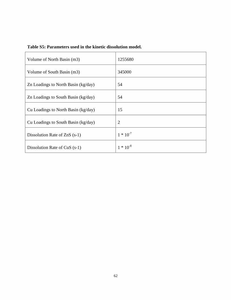
62
Table S5: Parameters used in the kinetic dissolution model.
Volume of North Basin (m3) 1255680
Volume of South Basin (m3) 345000
Zn Loadings to North Basin (kg/day) 54
Zn Loadings to South Basin (kg/day) 54
Cu Loadings to North Basin (kg/day) 15
Cu Loadings to South Basin (kg/day) 2
Dissolution Rate of ZnS (s-1) 1 * 10-7
Dissolution Rate of CuS (s-1) 1 * 10-8

63
Appendix 2: Supporting Information for Chapter 3
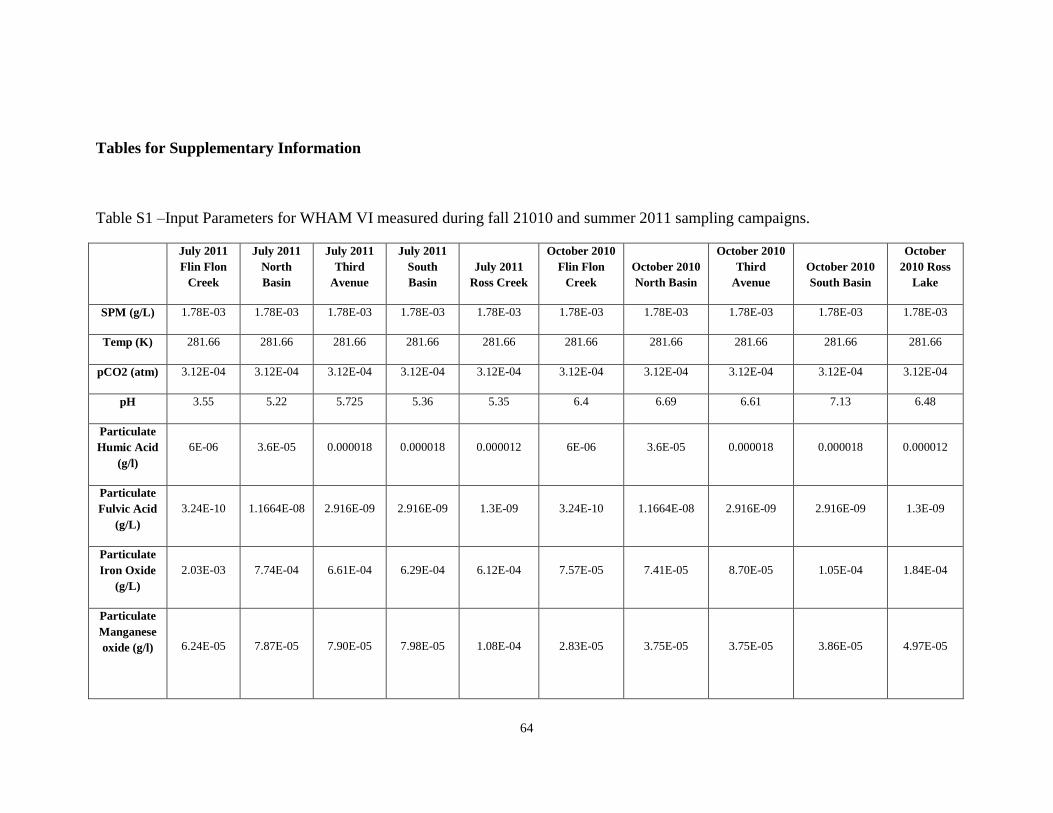
64
Tables for Supplementary Information
Table S1 –Input Parameters for WHAM VI measured during fall 21010 and summer 2011 sampling campaigns.
July 2011
Flin Flon
Creek
July 2011
North
Basin
July 2011
Third
Avenue
July 2011
South
Basin
July 2011
Ross Creek
October 2010
Flin Flon
Creek
October 2010
North Basin
October 2010
Third
Avenue
October 2010
South Basin
October
2010 Ross
Lake
SPM (g/L) 1.78E-03 1.78E-03 1.78E-03 1.78E-03 1.78E-03 1.78E-03 1.78E-03 1.78E-03 1.78E-03 1.78E-03
Temp (K) 281.66 281.66 281.66 281.66 281.66 281.66 281.66 281.66 281.66 281.66
pCO2 (atm) 3.12E-04 3.12E-04 3.12E-04 3.12E-04 3.12E-04 3.12E-04 3.12E-04 3.12E-04 3.12E-04 3.12E-04
pH 3.55 5.22 5.725 5.36 5.35 6.4 6.69 6.61 7.13 6.48
Particulate
Humic Acid
(g/l)
6E-06 3.6E-05 0.000018 0.000018 0.000012 6E-06 3.6E-05 0.000018 0.000018 0.000012
Particulate
Fulvic Acid
(g/L)
3.24E-10 1.1664E-08 2.916E-09 2.916E-09 1.3E-09 3.24E-10 1.1664E-08 2.916E-09 2.916E-09 1.3E-09
Particulate
Iron Oxide
(g/L)
2.03E-03 7.74E-04 6.61E-04 6.29E-04 6.12E-04 7.57E-05 7.41E-05 8.70E-05 1.05E-04 1.84E-04
Particulate
Manganese
oxide (g/l)
6.24E-05 7.87E-05 7.90E-05 7.98E-05 1.08E-04 2.83E-05 3.75E-05 3.75E-05 3.86E-05 4.97E-05

65
Colloidal
Humic Acid
(g/L)
0.000444 0.000414 0.000402 0.000408 0.000426 0.000444 0.000414 0.000402 0.000408 0.000426
Colloidal
Fulvic Acid
(g/L)
0.003996 0.003726 0.003618 0.003672 0.003834 0.003996 0.003726 0.003618 0.003672 0.003834
Total
Na(M) 3.18E-03 2.80E-03 2.78E-03 2.64E-03 2.63E-03 1.42E-03 1.02E-03 1.18E-03 9.87E-04 1.04E-03
Total
Mg(M) 6.38E-04 5.02E-04 5.97E-04 5.14E-04 5.88E-04 4.07E-04 3.72E-04 3.85E-04 3.62E-04 3.53E-04
Total K(M) 2.63E-04 2.28E-04 2.27E-04 2.28E-04 2.16E-04 1.56E-04 1.51E-04 1.52E-04 1.51E-04 1.53E-04
Total Ca
(M) 9.63E-03 8.23E-03 8.68E-03 8.01E-03 8.36E-03 4.67E-03 4.04E-03 4.24E-03 3.94E-03 4.04E-03
Total Mn
(M) 7.17E-07 9.05E-07 9.08E-07 9.17E-07 1.24E-06 3.26E-07 4.31E-07 4.31E-07 4.44E-07 5.72E-07
Total Cu
(M) 4.15E-07 6.94E-07 6.72E-07 6.74E-07 7.00E-07 6.92E-07 7.99E-07 8.48E-07 7.29E-07 7.52E-07
Total Cl
(M)
6.97E-03 5.50E-03 5.39E-03 5.36E-03 5.13E-03 6.97E-03 5.50E-03 5.39E-03 5.36E-03 5.13E-03
Total SO4
(M) 9.17E-03 7.53E-03 7.41E-03 7.35E-03 7.00E-03 3.43E-03 3.43E-03 3.62E-03 3.62E-03 3.62E-03
Total Zn
(M) 1.59E-06 5.78E-06 6.13E-06 6.03E-06 6.00E-06 3.12E-06 6.38E-06 6.09E-06 6.61E-06 7.60E-06

66
Table S2 –Input Parameters used for the single metal and metal mixture BLM, listed per location for fall 2010 and summer 2011 sampling campaigns.
pH Temp DOC HA
Ca -
Dissolved
Mg -
Dissolved
Na -
Dissolved
K -
Dissolved SO4 Cl Alkalinity
Cu -
Dissolved
Zn -
Dissolved
Al -
Dissolved
Ag -
Dissolved
As -
Dissolved
Co -
Dissolved
Cd -
Dissolved
Ni -
Dissolved
Pb -
Dissolved
Fe -
Dissolved
Location Date Media
degrees
C mgC/L (%) mg/L mg/L mg/L mg/L mg/L mg/L
mg/L
CaCO3 mg/L (mg/L) (mg/L) (mg/L) (mg/L) (mg/L) (mg/L) (mg/L) (mg/L) (mg/L)
Flin Flon
Creek Jul-11
Water
Column 3.55 22.82 7.4 10 439 16.6 74.5 10.4 881 247 <1.0 0.0197 0.0991 0.0436 <0.00010 0.00962 0.00070 0.000581 <0.0010 0.00246 1.20
North Basin Jul-11
Water
Column 5.22 21.68 6.9 10 321 12.2 56.2 8.71 723 195 2.6 0.0358 0.365 0.0389 <0.00010 0.00394 0.00089 0.00263 <0.0010 0.00132 0.24
Third Avenue Jul-11
Water
Column 5.72 22.60 6.7 10 319 14.9 54.2 8.53 712 191 3.4 0.0344 0.391 0.0348 <0.00010 0.00399 0.00091 0.00277 <0.0010 0.000985 0.18
South Basin Jul-11
Water
Column 5.36 21.61 6.8 10 313 12.4 53.4 8.91 706 190 3.3 0.0341 0.383 0.0343 <0.00010 0.00397 0.00090 0.00268 <0.0010 0.000975 0.18
Ross Creek Jul-11
Water
Column 5.35 22.59 7.1 10 310 14.8 53.8 8.14 672 182 6.9 0.00501 0.320 0.0330 <0.00010 0.00424 0.00092 0.000348 <0.0010 0.000256 0.13
Flin Flon
Creek
Oct-
10
Water
Column 6.4 9.32 7.4 10 179 7.76 33.1 6.1 329.6 247 3.2 0.0358 0.205 0.0243 <0.00010 0.0038 0.0005 0.00122 0.0036 0.000482 <0.010
North Basin
Oct-
10
Water
Column 6.69 10.17 6.9 10 166 6.81 27 5.94 335 195 3.2 0.0287 0.436 0.0214 <0.00010 0.00459 0.00083 0.00201 0.0029 0.000617 <0.010
Third Avenue
Oct-
10
Water
Column 6.61 10.11 6.7 10 164 7.05 28.4 6.04 347.4 191 3.2 0.0296 0.403 0.0217 <0.00010 0.0045 0.0008 0.00199 0.0038 0.000607 <0.010
South Basin
Oct-
10
Water
Column 7.13 10.35 6.8 10 161 6.74 26.6 5.9 335 190 3.2 0.0246 0.465 0.0191 <0.00010 0.00455 0.00087 0.00194 0.0032 0.000661 <0.010
Ross Creek
Oct-
10
Water
Column 6.48 10.30 7.1 10 158 7.27 26.7 6.03 335 182 3.2 0.0202 0.51 0.0205 <0.00010 0.00459 0.00084 0.00251 0.004 0.000594 <0.010

67
Appendix 3: Detailed Report on Analytical Methods, Results and Quality Control


![EQUILIBRIUM STUDIES ON THE REMOVAL OF ZINC(II) USING ... · from aqueous solutions [1981,2001]. The Zinc element is present in aqueous solutions mainly in the divalent states. Zinc](https://img.dokumen.tips/doc/110x75/5f1827d0583d9a2dd72adcb1/equilibrium-studies-on-the-removal-of-zincii-using-from-aqueous-solutions.jpg)


![Green synthesis of zinc oxide nanoparticles from aqueous ...€¦ · ZnO nanoparticles. Application of Zinc nitrate in synthesis of ZnO-NPs were reported by Diallo et al. [35] in](https://img.dokumen.tips/doc/110x75/5ed694fb843ed9152066a6b9/green-synthesis-of-zinc-oxide-nanoparticles-from-aqueous-zno-nanoparticles.jpg)