EXAMENSARBETEN I MATEMATIKMATEMATISKA INSTITUTIONEN, STOCKHOLMS UNIVERSITET

Transient identification at nuclear power plants using

support vector machines

av

Christoffer Gottlieb

2004 - No 18

MATEMATISKA INSTITUTIONEN, STOCKHOLMS UNIVERSITET, 106 91 STOCKHOLM

Transient identification at nuclear power plants usingsupport vector machines

Christoffer Gottlieb

Examensarbete i matematik 20 poang

Handledare: Vasily Arzhanov och Wac�law Gudowski

2004

Transient Identification at Nuclear Power Plants using Support Vector Machines

Christoffer Gottlieb Thesis in Applied Mathematics

Written for the

Mathematics Department, University of Stockholm

At and In Co-operation with the Reactor Physics Department,

Royal Institute of Technology, Stockholm

Supervisors: Vasily Arzhanov and Waclaw Gudowski

2004

ii

Abstract

In this thesis, Support Vector Machines (SVMs), a relatively new paradigm in learning machines, are studied for their potential to recognize transient behavior of sensor signals corresponding to various accident events at Nuclear Power Plants (NPPs). Transient classification is a major task for any computer-aided system for recognition of various malfunctions. The ability to identify the state of operation or events occurring at a NPP is crucial so that personnel can select adequate and swift response actions. Modular Accident Analysis Program (MAAP4) is a software program that can be used to model various normal and abnormal events at a NPP. A previous study used MAAP4 to simulate various accident events (pipe ruptures) at boiling water reactors (BWR). In the main experiment of this thesis, the simulated sensor readings corresponding to these events have been used to train and test SVM classifiers. SVM calculations have demonstrated that they can produce classifiers with good generalization ability for our specific formulation of the learning problem. This in turn indicates that SVMs show promise as classifiers for the learning problem of identifying transients. A significant portion of the effort spent in this thesis went into examining SVMs and the underlying theory, Statistical Learning Theory (SLT).

iii

iv

Acknowledgements

I would like to acknowledge the financial support of the Swedish Nuclear Power Inspectorate (SKI) and thank Ninos Garis (at SKI) for initiating the project. Furthermore, I would like to express my boundless gratitude to Waclaw Gudowski for entrusting me with this responsibility and Vasily Arzhanov for his continual support and personal sacrifice. I would like to thank both supervisors for the many fruitful discussions we had and for their high expectations both in quality and scope. Alexandra Ålhander for being a fun roommate, for sharing the trials and tribulations of writing a thesis and for putting up with the bananas. Mario Fritz for the many helpful emails he sent to a complete stranger. Finally, I would like to thank the remaining staff and students at the Nuclear and Reactor Physics Department at Albanova for providing an enjoyable work environment.

v

vi

Dedication

To my wonderful family

vii

viii

Table of Contents 1 Introduction................................................................................................................. 1

1.1 Transient States................................................................................................... 1 1.2 Classification of Reactor Events......................................................................... 2 1.3 Criteria of Reactor State Monitoring Systems .................................................... 4 1.4 History of Transient Identification at NPPs........................................................ 4

2 Statistical Learning Theory......................................................................................... 6 2.1 Notation Used ..................................................................................................... 6 2.2 Learning Machines.............................................................................................. 7 2.3 Vapnik-Chervonenkis Theory............................................................................. 8 2.4 Empirical Risk Minimisation (ERM)................................................................ 10 2.5 Nontrivial Consistency...................................................................................... 10 2.6 The Key Theorem of Learning Theory............................................................. 12 2.7 Concepts of Capacity ........................................................................................ 13 2.8 Conditions for Consistency............................................................................... 15 2.9 Bounds on the Rate of Convergence................................................................. 16 2.10 Bounds on the Generalization Ability of Learning Machines .......................... 17 2.11 Constructive Bounds of the Generalization Ability.......................................... 19 2.12 Structural Risk Minimisation (SRM)................................................................ 20

3 Support Vector Machines ......................................................................................... 23 3.1 The Linear Separable Case ............................................................................... 23 3.2 The Linear Non-separable Case........................................................................ 27 3.3 The Non-Linear Case........................................................................................ 28

4 Experiments .............................................................................................................. 31 4.1 Phase 1 – Manually Generated Data................................................................. 31

4.1.1 Structure of Experiment............................................................................ 31 4.1.2 Signal Prototypes ...................................................................................... 32 4.1.3 Generation of Training and Test Sets ....................................................... 34 4.1.4 Addition of Gaussian Noise ...................................................................... 34 4.1.5 Normalising Training and Test Sets ......................................................... 35 4.1.6 Implementation of SVM Methodology..................................................... 36 4.1.7 Implementation of NN Methodology........................................................ 37 4.1.8 Test Runs .................................................................................................. 40 4.1.9 Results....................................................................................................... 41 4.1.10 Conclusion ................................................................................................ 44

4.2 Phase 2 – MAAP Simulated Data..................................................................... 45 4.2.1 The MAAP Signals ................................................................................... 45 4.2.2 Problem Formulation ................................................................................ 51 4.2.3 Noise Simulation....................................................................................... 51 4.2.4 Signal Pre-processing................................................................................ 52 4.2.5 Parameter Design ...................................................................................... 52 4.2.6 Software Implementation.......................................................................... 54 4.2.7 Results....................................................................................................... 54 4.2.8 Conclusion ................................................................................................ 57

5 Summary and Future Improvements......................................................................... 58

ix

6 References................................................................................................................. 60 A. Literature Review of Support Vector Machines ....................................................... 64

x

1 Introduction Nuclear power plants (NPPs) are run and controlled by a team of human operators. To assist them in their task they have to their disposal numerous sensors and indicators that monitor various components of the plant. The operators are responsible for the taking of appropriate actions in response to both normal events - such as minor disturbances, planned interruptions and transitions to different operational states; and abnormal events -such as major disturbances and actuator/instrumentation failures. For reasons such as safety and reduction of costs, it is important to detect and recognize these events within a given time frame. Even an experienced operator may be overwhelmed by signals and readings of a large number of sensors and alarms in case of unpredicted and abrupt events. That is why computerized monitoring systems have long been used at NPPs with the aim of not only displaying real-time histories of various sensors but to also automatically identify transients and then classify them as specific events. These computerized monitoring systems are often based on methods suited for problems of pattern recognition. M. Bednarski’s Msc. thesis [1] studied how three interpolation algorithms could be applied to the problem of correctly classifying accident sequences to the kind of accident event that triggered them. Accident sequences are identified by the particular transient states that occur in response to the event. This paper continues this investigation using Support Vector Machines (SVMs). The work conducted in this thesis can be divided into three main stages. 1) Develop an understanding of the underlying theory of SVMs and the framework in which it lays - Statistical Learning Theory. 2) Conduct test runs with simulated signals in which SVM performance is assessed. 3) A preliminary attempt at comparing SVMs to Artificial Neural Networks (ANNs).

1.1 Transient States In order to understand the concept of a transient state let us begin by looking at a definition of the everyday word. transient 1. Passing before the sight or perception, or, as it were, moving over or across a space or scene viewed, and then disappearing; hence, of short duration; not permanent; not lasting or durable; not stationary; passing; fleeting; brief; transitory. 2. Hasty, momentary; imperfect: brief. 3. Staying for a short time; not regular or permanent.

Webster’s Revised Unabridged Dictionary (1998) The following paragraph adjusts the definition to the context of signal analysis.

1

A great majority of industrial processes (including NPPs) are characterised by long periods of steady-state operation interrupted occasionally by shorter periods of dynamic behaviour. These periods of dynamic behaviour are referred to as transient states. Events that occur in the operation of nuclear reactors are characterized by transient states. These transients manifest themselves in the numerous signals that monitor various NPP components. The detection and identification of transient states are important steps in the diagnosis and mitigation of potential accident events. This is often nontrivial as a particular transient state can characterize many events. Furthermore, several events can occur within a small time frame, causing an overlapping of many transients that are often hard to distinguish.

Figure 1. Signal readings of some arbitrary process moving from one period of steady-state operation to another.

Solutions to the steps described above can be categorized into two main approaches. The first solution involves comparisons of the signal to a knowledge base of known transient identifier patterns (empirical model). The second infers information about the signal from a knowledge base containing a qualitative model of the NPP. Some solutions combine these two approaches so that they work alongside each other. In the context of SVMs we deal with solutions of the first kind.

1.2 Classification of Reactor Events Reactor events or states can be categorized on the basis on the frequency of their occurrences. In [1], M. Bednarski listed the following classification of reactor states based on the U.S. Nuclear Regulatory Commission’s Code of Federal Regulations (Part 50) [2].

2

Class 1 Reactor states occurring frequently and regularly during normal operation, refueling and maintenance. Examples: • Start of reactor. • Shutdown of reactor. • Operation with some systems switched off due to repair or testing. • Faults of fuel can not exceeding admissible limits. Class 2 Reactor states occurring at moderate frequency during operation of the plant. Examples: • Inadvertent pulling out of control rods. • Partial cut-off of forced circulation in the rod (e.g. as a consequence of blocking of

recirculation pumps). • Ensealing due to false operation of an element, e.g. valve. • Single fault of the operator. • Single defect of a control element. • Loss of external power supply. Class 3 Reactor states occurring very rarely in the course of plant operation. Examples: • Loss of reactor cooling as a result of a minor damage to the pipe, resulting in reactor

shutdown (small LOCA – Loss-of-Coolant-Accident). • False operation of control rods. • Inadvertent insertion of fuel cassette in an improper position. • Inadvertent pulling out of a single control rod in the course of refueling. • Total interruption of forced circulation in the rod. Class 4 Accidents that should not happen but are taken into account by reason of potential consequences of radioactive products liberation. These states are the most severe ones, and are considered by reasons of safety. Examples: • Loss of cooling connected with major damage to the pipe (large LOCA). • Displacement of fuel. • Large damage to a pipe in the secondary circulation system (PWR reactors).

3

Class 3 and 4 reactor states have the most severe implications to safety during operations at nuclear power plants. Since they occur seldom human operators will have less real-life experience with them. Such states (or possibility of) may put operators in situations of considerable stress, increasing the risk of human error. The faster such reactor states are detected and identified, the more likely it is that operators will handle the situation correctly. The existence of computerized monitoring systems that can facilitate the detection/identification of reactor states of Class 3/Class 4 are therefore of high priority. This thesis deals with the classification of various water and steam pipe rupture which belong to Class 3 and Class 4 type states.

1.3 Criteria of Reactor State Monitoring Systems In the context of this thesis, a computerized monitoring system needs to fulfil two important criteria. 1) It needs to be accurate. It is important that the operators can put a high level of trust

in the predictions of the system. Such trust can only be built up on prior predictions that have been confirmed as accurate. Too many false alarms and misclassified events may lead to disastrous scenarios where operators disregard correct observations of severe reactor states simply because it has been wrong in many previous situations.

2) It needs to be fast enough to give operators a sufficient time frame in which to make corrective adjustments.

1.4 History of Transient Identification at NPPs Over the years, a variety of data-based and model-based computerized monitoring solutions have been proposed in identifying transients at nuclear power plants. In this research, a large portion of the solutions use artificial neural networks (ANNs). Among the first to examine the applicability of ANNs to this task were R. E. Uhrig and E. B. Bartlett in the late 80s [3]-[5]. These first attempts were based on feedforward backpropagation neural networks and were soon improved on with a variety of techniques. Some subsequent research addressed specific shortcomings of the aforementioned method. For instance, in [6], R. E. Uhrig and E. B. Bartlett proposed an important technique that allows classifiers to respond with “don’t-know” answers. Most research however tried to improve overall performance of the “simple” feedforward neural network. In [7], neural networks where incorporated into a modular hierarchy with a dynamic node architecture. Furthermore, hybrid solutions were studied using neural networks in conjunction with other soft computing methods. The solution in [8] used a connectionist expert system having neural networks for their knowledge bases. In [9], a hybrid neural network-fuzzy logic approach was studied and [10] combined observer-based residual generation with neural classifiers. However, the different methods used in the research mentioned up until now consider spatial variations and are insensitive to the underlying time dependency of transients in this problem domain. Neural network-based solutions that try to address the time dependency use NN architectures such as recurrent

4

multi-layer perceptrons [11], spatiotemporal NNs [12] and NNs with implicit time measure [13]. A particularly mature realization of transient identification using neural network classifiers is the Aladdin project ([14] and [15]), run and funded by OECD Halden Reactor Project (at the Institute for Energy Technology (IFE)). It combines ensembles of recurrent neural network classifiers with wavelet preprocessing [17] and autonomous recursive task decomposition (ARTD) [16]. It has shown good results and scales well to the demands of complex real-life applications. Methods for transient identification at NPPs that do not rely on neural networks include fuzzy logic [18], hidden Markov models [19], and nearest-neighbours modeling optimized by a genetic algorithm [20]. In terms of support vector machines, [21] integrated an adaptation of SVMs with a proprietary nonlinear and nonparametric technique - Multivariate State Estimation Technique (MSET).

5

2 Statistical Learning Theory

2.1 Notation Used n∈x - An input point from the input space (domain of the sought-after

function/dependencyx

( ),f αx ). y ∈ - Target or output point y (range of ( ),f αx ).

( ), ny = ∈ ×x z - An element of the training set.

( )1 2, , , nlS = ⊂z z z… × - Training set: the set of pairs of input points and

corresponding target values used when training a classifier. ( ), nb ∈ ×w - Parameters that define a hyperplane in 1n+ where is the normal vector of the hyperplane andb is the perpendicular Euclidian distance between the hyperplane and the origin.

w

, , n⋅ ∈x y x y - Scalar product between and x y .

( ){ },fα

α∈Λ

x - Set of functions from which a learning machine can choose one that best approximates the learning problem at hand (hypothesis space). w - Euclidean norm of w .

6

2.2 Learning Machines Learning machines is a general category ascribed to algorithms that on the basis of a set of rules and a training set return a function f from a set{ }( , )f

αα

∈Λx . In regression this

function (chosen from the set of possible functions{ }( , )fα

α∈Λ

x ) is nothing more than the one that best approximates the underlying dependence that has generated our data points. In classification, this sought-after function (discriminant function) returns an integer value representing the class of the input point. In statistical literature, the sought-after function is widely referred to as the hypothesis and the set of functions from which it can chose the hypothesis, the hypothesis space. The process in which algorithms choose the most appropriate function by manipulating a set of training points is often referred to as supervised learning. In classification, each input vector n∈x of the training set is associated with a target, a qualitative variable instance representing one of y Y∈ { }1, , nY y y= … possible classes. These classes indicate to which category each input point belongs to, and are normally represented by integer values. For example, binary classification (dichotomization), classify input data into one of two classes { }1 2,Y y y= and are generally represented

by{ }0,1 or { }1,1− . Each such pair ( ), yx will be regarded as random variables belonging

to some unknown joint probability distribution ( ),P yx . The problem examined in this thesis has been formulated as one of pattern recognition. The theoretical discourse ahead will therefore centre itself around results obtained for classification. To clarify the problem and formulation of classification consider the following example. A company needs to improve the way they identify faulty products in assembly. Their engineers have discovered that there seems to be an unknown dependency between certain product features and faulty/non-faulty products. Let us assume that the engineers have found two such features – weight ( 1x ) and size ( 2x ) of product for some unspecified scalar units. We will represent this feature pair as the vector ( )1 2,x x=x and see that it

constitutes an input point of the input space (see Figure 2). As supervised learning algorithms rely on a training set of known values, the engineers record the weight and size of products and determine whether these products are faulty or not. The class of faulty products is associated with the value of

2

l1− and non-faulty products with the value

of1. Each feature vector is paired up with a value that correctly labels the state of the product and the resulting training set

x y

( ) ( ) ( )( ) ( )21 1 2 2, , , , , ,l lS y y y Y= ⊂ ×x x x… is

used to find the best discriminant function ( ),f αx . The resulting function can then be used to predict the class of a product by merely measuring the weight and size of it. New input points will be classified to one of the two classes by looking at what region of the input space they belong to. Provided that ( ),f αx is good approximation of the underlying dependency the company can now rely on the predictions of the trained classifier and can to some degree circumvent the laborious task of manually inspecting each product.

7

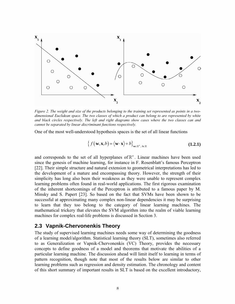
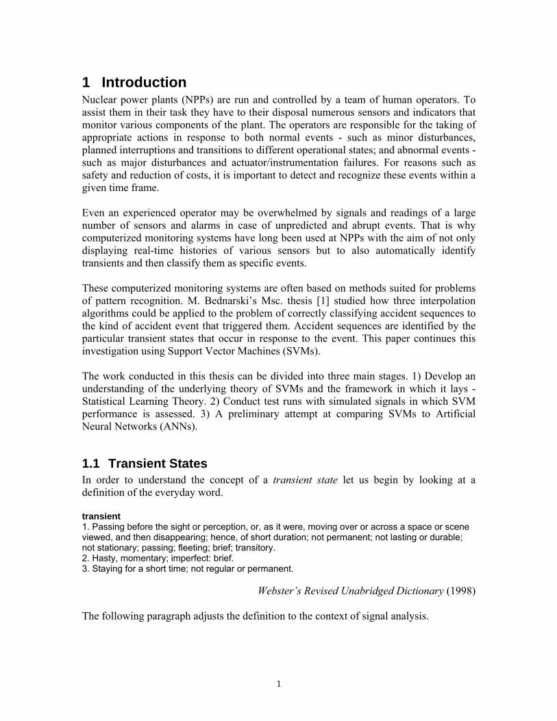
Figure 2. The weight and size of the products belonging to the training set represented as points in a two-dimensional Euclidean space. The two classes of which a product can belong to are represented by white and black circles respectively. The left and right diagrams show cases where the two classes can and cannot be separated by linear discriminant functions respectively.

One of the most well-understood hypothesis spaces is the set of all linear functions ( ){ } ,

, , n bf b b

∈ ∈= ⋅ +

ww x w x (1.2.1)

and corresponds to the set of all hyperplanes of . Linear machines have been used since the genesis of machine learning, for instance in F. Rosenblatt’s famous Perceptron [22]. Their simple structure and natural extension to geometrical interpretations has led to the development of a mature and encompassing theory. However, the strength of their simplicity has long also been their weakness as they were unable to represent complex learning problems often found in real-world applications. The first rigorous examination of the inherent shortcomings of the Perceptron is attributed to a famous paper by M. Minsky and S. Papert [23]. So based on the fact that SVMs have been shown to be successful at approximating many complex non-linear dependencies it may be surprising to learn that they too belong to the category of linear learning machines. The mathematical trickery that elevates the SVM algorithm into the realm of viable learning machines for complex real-life problems is discussed in Section 3.

n

2.3 Vapnik-Chervonenkis Theory The study of supervised learning machines needs some way of determining the goodness of a learning model/algorithm. Statistical learning theory (SLT), sometimes also referred to as Generalization or Vapnik-Chervonenkis (VC) Theory, provides the necessary concepts to define goodness of a model and theorems that motivate the abilities of a particular learning machine. The discussion ahead will limit itself to learning in terms of pattern recognition, though note that most of the results below are similar to other learning problems such as regression and density estimation. The chronology and content of this short summary of important results in SLT is based on the excellent introductory,

8

inspiring and philosophically acute book by V. N. Vapnik [24] - a central figure in the founding of SLT. Many of the definitions and theorems of this section have been reproduced from this book. Let be a training set andS ( ), , f α α ∈ Λx the hypothesis space from which the learning machine chooses the function that best describes the dependency between random variables X andY . The training set consists of independently and identically distributed (i.i.d.) training data from some unknown joint probability

distribution . Since the discussion ahead limits itself to that of classification each

is assigned one of n labels from the set of classes

( ), , 1,i iy i =x …l

)( ,P yx

iy { }1, , nY Y Y= … . In general, classes are represented by unique integer values. In search of the best model we need to define a concept of goodness so as to be able to discriminate between different learning models. Furthermore, this concept will allow us to select the best hypothesis for a specific hypothesis space. The central concept of goodness is the generalization ability of a learning machine, i.e. its ability to generalize from a set of known to unknown values of the dependency in question. A trained learning machine’s ability to generalize is evaluated by a set of input points not used in the training phase – a test set. This is formalised by the introduction of a loss function ( , ( , ))L y f αx which defines the experienced loss (discrepancy) given the learning machines response ( , )f αx and actual value . Defining the risk functional y ( ) ( )( ) ( )( ), , ( , ) , ,R f L y f dP y E L y fα α⎡ ⎤= = ⎣ ⎦∫ x x x (1.3.1) we are given the expected predication error when generating data from the probability distribution . In other words, given hypothesis( , )P yx ( ){ },f f

αα

∈Λ∈ x , the average error

(as defined by the loss function) is ( )R f . This risk functional is called the generalization error or test error. Choosing an appropriate loss function generally depends on the context of the learning problem. The simplest and often used loss functions for classification is the 0 loss function, 1−

( )( ) ( )(

1 if ,, ,

0 if , .

y fL y f

y f )α

αα

≠⎧⎪= ⎨=⎪⎩

xx

x (1.3.2)

From the definition above we see that a penalty (of value 1) is assigned when a misclassification occurs, while correct classifications incur no penalty. If the joint probability density function is known it is often possible to analytically minimize the generalisation error for a chosen loss function. Unfortunately, in most real-life

( ,P yx )

9

learning problems the training points are too few to establish the underlying probability distribution of the data. The problem of learning can therefore be seen as “minimising the risk functional ( )R f on the basis of empirical data” ([24], p.18). In order to do so, several inductive principles can be employed with varying degrees of success to generalise. Different inductive principles have different pre-requisites regarding the amount of information known about the underlying joint probability distribution ( ),P yx . This paper will describe inductive principles important in the context of SVMs – Empirical Risk Minimisation (ERM) and Structural Risk Minimisation (SRM).

2.4 Empirical Risk Minimisation (ERM) Classical solutions to learning and statistical problems such as the least-squares method and the maximum likelihood method are both realisations of the ERM principle. Its history (in terms of learning problems) stretches back to theorems about properties of the Perceptron by A. B. J. Novikoff [25] in the early 60’s. In that era, the ERM was considered to be the inductive principle with best generalisation ability. This view was however based on intuition rather than theoretical results. Statistical learning theory demonstrates the limitations of ERM (especially when faced with few training points) and introduces inductive principles with better generalisation abilities. In ERM, the risk functional (expected prediction error) is replaced by the empirical risk functional,

( ) ( )(1

1 , ,l

emp i ii

R L y fl

).α α=

= ∑ x (1.4.1)

The function with minimal risk is approximated by the function that gives minimal empirical risk, and depends on the specific points in the training set. This often overly optimistic approximation has been superseded by better methods such as Akaike Information Criterion (AIC), Bayesian Information Criterion (BIC), Minimum Description Length (MDL) (see [26] pp. 193-222 for a good review) and Structural Risk Minimisation (SRM) (which will be covered further on in the text).

2.5 Nontrivial Consistency Learning machines that are based on the ERM principle do not always have small actual risk (test error). Theory was therefore developed (largely by Vapnik and Chervonenkis [27], [28], [29]) so as to indicate when a specific learning machine based on ERM can generalise well and when it cannot. In the case when it can generalise well we say that the learning machine is consistent with the ERM principle. Statistical learning theory presents necessary and sufficient conditions for consistency. For the sake of brevity ( ) ( ) ( )1 1 2 2, , , , , ,l ly yx x x… y

10

will from now on be denoted with and1 2, , , lz z z… ( )( ), ,L f yαx by ( ),Q αz .

Figure 3. Illustration of the definition of consistency.

Definition Let ( , lQ )αz be the loss function that minimises the empirical risk ( )empR α given observations . We say that the ERM principle is consistent for the set of functions (learning machine)

1 2, , , lz z z…( ), , Q α α ∈ Λz and probability distribution function ( )P z if

the following two sequences converge in probability to the same limit. ( ) ( )inf ,P

l lRα

Rα α→∞ ∈Λ⎯⎯⎯→ (1.5.1)

( ) ( )inf .P

emp l lRα

Rα α→∞ ∈Λ⎯⎯⎯→ (1.5.2)

However, this definition of consistency falls prey to cases of trivial consistency. This condition can be obtained by taking any set of loss functions ( ), , Q α α ∈ Λz that is not

consistent with the ERM principle and adding a function ( )φ z to this set such that ( ) ( )inf , , Q

αα φ

∈Λ>z z ∀z (1.5.3)

As Figure 4 tries to illustrate, any such set containing a minorizing function will make the ERM principle consistent. Sets such as these would force any theory of consistency to inspect learning machines for cases of trivial consistency. This

( )φ z

11

unnecessarily unpractical procedure is circumvented by extending the definition of consistency.

Figure 4. An example of trivial consistency where a minorizing function ( )φ z is included in the set of

functions . ( ), ,Q α α ∈ Λz

Definition1 The ERM principle is nontrivially consistent for the set of functions and for the probability distribution function( ), , Q α α ∈ Λz ( )P z if for any

nonempty subset of this set of functions defined as ( ) ( ), ,c cΛ ∈ −∞ ∞ ( ) ( ) ( ){ }: , , c Q dP cα α αΛ = > ∈ Λ∫ z z (1.5.4) the convergence ( )

( )( )

( )inf infPemp lc

Rα α c

Rα α→∞∈Λ ∈Λ⎯⎯⎯→ (1.5.5)

is valid. In studying whether the ERM principle is nontrivially consistent for specific learning machines we are able to learn more about the generalisation properties of a specific learning method.

2.6 The Key Theorem of Learning Theory A breakthrough in the study of nontrivial consistency came in 1989 when V. N. Vapnik and A. Ja. Chervonenkis [30] formulated and proved the key theorem of learning theory.

1 This definition applies to our problem of pattern recognition/classification. For an equivalent definition for density estimation see p.37 in [24].

12

Key Theorem of Learning Theory Let ( ), , Q α α ∈ Λz be a set of functions that satisfy the condition ( ) ( ) ( )( ), A RA Q dP B Bα≤ ≤ ≤∫ z z α ≤ (1.6.1) Then for the ERM principle to be consistent, it is necessary and sufficient that the empirical risk ( )empR α converge uniformly to the actual risk ( )R α over the

set in the following sense, ( ), , Q α α ∈ Λz

( ) ( )( ){ }lim sup 0, 0.emplP R R

αα α ε ε

→∞ ∈Λ− > = ∀ > (1.6.2)

This important theorem shows that the study of nontrivial consistency is equivalent to the study of the problem of uniform one-sided convergence as presented in the theorem above. Eq. (1.6.2) show how consistency is determined by the worst function of the set of loss functions. So any analysis of the ERM principle for a learning machine must be a “worst case analysis”. This put an end to the ambitions of a particular school of researchers that hoped for results allowing “real case analysis”. This fact was noted by V. N. Vapnik in [24], p. 37.

2.7 Concepts of Capacity Finding conditions for when Eq. (1.6.2) holds are therefore of central importance as it provides necessary and sufficient conditions for nontrivial consistency. To find such conditions, the concept of capacity or diversity of a set of functions was introduced. One such concept of capacity is the entropy of a set of functions. Below we define entropy for a set of indicator functions (which is sufficient for pattern classification when using the 0-1 loss function). For a generalisation of the concept of entropy for sets of real-valued functions see [31], pp. 98-99. Definition Let be a set of indicator functions and consider an i.i.d.

sample generated by some probability distribution function . Now consider the set of -dimensional binary vectors

( ), , Q α α ∈ Λz

1 2, , , lz z z… ( )P zl

( ) ( ) ( ) ( )( )1 2, , , , , , , lq Q Q Qα α α α α= ∈z z z… Λ . (1.7.1) The number of unique ( )q α constructed in this manner is the entropy with respect

to and , and is denoted by( ), , Q α α ∈ Λz 1 2, , , lz z z… ( )1 2, , , lN Λ z z z… . It evaluates how many different separations of the given sample can be done using functions

13

from . Geometrically speaking, it is the number of different vertices of the -dimensional unit cube that can be obtained.

( ), , Q α α ∈ Λzl Entropy for sets of real-valued functions depends on the additional variableε and is denoted by . All results below use the more general concept of entropy for real-valued functions but are valid for sets of indicator functions.

( 1 2; , , , lN εΛ z z z… )

The concept of entropy is modified in several ways to provide the following constellation of related concepts.

( ) ( )( ) ( )

( ) ( )( ) ( )

1

1 1

1

1

1, ,

; , , ln ; , , (VC Random Entropy)

; ; , , (VC Entropy)

ln ; , , (Annealed VC Entropy)

ln sup ; , , (Growth Function)l

l l

l

ann l

l

H N

H l E H

H l E N

G l N

ε ε

ε ε

ε

ε

Λ Λ

Λ Λ

Λ Λ

Λ Λ

=

⎡ ⎤= ⎣ ⎦⎡ ⎤= ⎣ ⎦

=z z

z z z z

z z

z z

z z…

… …

…

…

…

(1.7.2)

Using this family of concepts, conditions have been formulated that provide sufficient and/or necessary conditions for the uniform one-sided convergence, and hence also the original question of non-trivial consistency of the ERM principle. These will be introduced in the next section. A more important capacity concept from a practical point of view is the Vapnik-Chervonenkis (VC) dimension. Definition (indicator functions) The VC dimension of the set of indicator functions

( ){ },fα

α∈Λ

x is the maximum number of vectors that can be separated into two

classes in all possible ways using functions of the set. We say that the set of vectors have been shattered by the set of functions. If for any n , there exists a set of vectors which can separated into two classes in all possible ways we say that the VC dimension of the set is equal to infinity.

h , , h1x x…

2h

n2h

The VC dimension for a set of real functions is given by constructing a set of indicator functions from the set of real functions in the following manner. Definition (real functions) Let ( ), , A f Bα α≤ ≤ ∈x Λ be a set of real functions bounded by the constants A and B . Construct a set of indicator functions from the set of real functions as following, ( ) ( )( ) ( ), , , , , ,I fα β θ α β α β= − ∈ Λ ∈x x A B (1.7.3) where is the step-function ( )uθ

14

( )0 if 01 if 0.

zu

zθ

<⎧= ⎨ ≥⎩

The VC dimension of a set of real functions ( ), , A f Bα α≤ ≤ ∈x Λ is defined to be the VC dimension of the set of corresponding indicator functions (1.7.3) with parametersα ∈ Λ and ( ),A Bβ ∈ . Theorem Consider some set of points in . Choose any one of these points as origin. Then the points can be shattered by orientated hyperplanes i.f.f. the position vectors of the remaining points are linearly independent.

m n

m

A corollary of this theorem is that the VC dimension of the set of orientated hyperplanes in is . The VC dimension of a set of linear discriminant functions is therefore easy to determine from the dimensionality of the input/feature space of the learning problem. This is important as the VC dimension is used to provide bounds on the actual risk of discriminant functions as is shown in subsequent sections.

n 1n +

Figure 5. Left – Three points in that can be shattered with orientated hyperplanes. This shows that the VC dimension is at least 3. Right – Different arrangements of four points in labelled in such a way that no hyperplane can separate the two classes. Such a labelling exists for any four points in .

2

2

2

2.8 Conditions for Consistency With the help of the capacity concepts introduced in the previous section V. N. Vapnik and A. Ja. Chervonenkis derived equations that describe conditions for consistency of the ERM principle. The first equation of significance was one that uses the VC entropy to describe a sufficient condition for consistency and states that consistency is meet if

( )lim 0

l

H ll

Λ

→∞= (1.8.1)

15

holds true. However, this equation does not say anything about the asymptotic convergence rate of the obtained risks ( )lR α to the minimal risk ( )0R α and examples have been constructed where this rate is arbitrarily slow. To amend this apparent weakness it was first necessary to provide a definition of a fast convergence rate. Definition We say that the asymptotic rate of convergence is fast if for any , the exponential bound

0l l>

( ) ( ){ } 2

0c l

lP R R e εα α ε −− > < holds true, where is some constant. 0c > It has been shown that a sufficient condition for a fast rate of convergence is the following equation

( )lim 0.ann

l

H ll

Λ

→∞= (1.8.2)

As both the VC entropy ( )H lΛ and annealed VC entropy ( )annH lΛ depend on the sample

they depend on the probability distribution1 2, , , lz z z… ( )P z . The sufficient conditions given above for consistency Eq. (1.8.1), and consistency with a fast convergence rate Eq. (1.8.2) are therefore distribution dependent. To generalise these results for any distribution it was shown that necessary and sufficient conditions for consistency independent of the probability distribution with a fast convergence rate is satisfied when

( )lim 0.

l

G ll

Λ

→∞= (1.8.3)

The three equations (1.8.1), (1.8.2) and (1.8.3) are referred to by V. N. Vapnik ([24], pp. 52-54) as the first, second and third milestones of learning theory. Next, we will see how these equations can be used to formulate bounds on the rate of convergence, and more importantly, on the actual risk of learning machines.

2.9 Bounds on the Rate of Convergence V. N. Vapnik and A. Ja. Chervonenkis (see Chapters 4-5 in [31]) showed that the annealed VC entropy ( )annH lΛ and growth function ( )G lΛ can be used to provide distribution-dependent and distribution-independent bounds on the rate of convergence, respectively. The following theorem below presents an inequality that gives a bound on the rate of convergence on a set of indicator functions ( ), , Q α α ∈ Λz . Similar bounds are available for set of real-valued functions but are beyond the scope of this paper.

16

Theorem For a set of indicator functions ( ), , Q α α ∈ Λz , sample and for any

1 2, , , lz z z…0ε > the following inequality holds true:

( )( ) ( ) ( )( ) ( ) 2

1

21sup , , , , , 4exp .l

anni i

i

H lP L y f dP y L y f

l lαα α ε

Λ

∈Λ =

lε⎧ ⎫⎛ ⎞⎧ ⎫ ⎪ ⎪− > ≤ ⎜ ⎟⎨ ⎬

⎩ ⎭ ⎝ ⎠⎩ ⎭∑∫ x x x −⎨ ⎬

⎪ ⎪(1.9.1)

If Eq. (1.8.2) holds then clearly we are guaranteed that for any 0ε > , the right-hand side will go to 0 as l . We say that the bound is non-trivial. As→ ∞ ( )annH lΛ depends on the

sample’s distribution the theorem above gives us a distribution-dependent bound on the rate of convergence. To obtain a similar distribution-independent bound we use the fact that

( )P z

( ) ( ) ( ).annH l H l G lΛ Λ Λ≤ ≤

( )G lΛ is distribution-independent and when substituted into Eq. (1.9.1) gives a distribution-independent bound. Similarly, if the third milestone of learning theory, Eq. (1.8.3), holds the bound will be non-trivial. However, note that the third milestone, if satisfied, provides necessary and sufficient conditions for the ERM principle to be consistent. This stronger result implies that any set of indicator functions that does not satisfy Eq. (1.8.3) will result in a trivial bound in Eq. (1.9.1). This in turn guarantees the existence of probability distribution functions for which the uniform convergence of Eq. (1.9.1) does not take place.

2.10 Bounds on the Generalization Ability of Learning Machines To describe the generalisation ability of a learning machine based on the ERM principle Vapnik ([24] pp.72) identifies two questions that need to be answered:

1. What actual risk ( lR )α is provided by the function ( ), lQ αz that achieves minimal

empirical risk ( )emp lR α ?

2. How close is this risk to the minimal possible ( )inf Rα

α∈Λ

, for the given set of

functions? Both these questions can be answered with inequalities equivalent to the bound given in eq. (1.9.1). The equivalence is apparent but is derived below as part of an exercise. Once again, these bounds are valid for sets of indicator functions and present distribution-independent bounds. Similar results are available for sets of real-valued functions. (Question 1) The distribution-independent version of eq. (1.9.1) is

17

( ) ( ){ } ( ) 22sup 4expemp

G lP R R l

lαα α ε ε

Λ

∈Λ

⎛ ⎞⎛ ⎞− > ≤ −⎜⎜⎜⎝ ⎠⎝ ⎠

⎟⎟ ⎟ . (1.10.1)

Let

( ) ( )

22 ln2 44exp

G lG ll

l l

η

η ε εΛ

Λ −⎛ ⎞⎛ ⎞= − ⇔ =⎜ ⎟⎜ ⎟⎜ ⎟⎝ ⎠⎝ ⎠

.

Then for all indicator functions ( ), , Q α α ∈ Λz the following inequality holds with probability of at least1 η− : ( ) ( ) ( ) ( )sup emp empR R R R

αα α ε α α

∈Λ− ≤ ⇒ − ε≤

This is equivalent to

( ) ( )

( ) ( )and

emp

emp

R R

R R

α α ε

α ε α

≤ +

− ≤ (1.10.2)

As Eq. (1.10.2) holds for all α ∈ Λ it answers question 1 by providing bounds on ( )lR α in terms of the empirical risk, number of samples and Growth function. (Question 2) Let lα ∈ Λ be the indicator function that achieves minimal risk and 0α ∈ Λ the indicator function with minimal actual risk. From Eq. (1.10.2) and [31] ( p. 124 ) we know that the following inequalities hold with probability of at least1 η−

( ) ( )

( ) ( )0 0ln2

l emp l

emp

R R

R Rl

α α ε

ηα α

≤ +

−> −

(1.10.3)

By definition ( ) ( )0emp l empR Rα α≤ , giving

( ) ( )0ln2emp lR Rlηα α −

> − . (1.10.4)

By subtracting the left-side and right-side of inequality (1.10.4) with the left-side and right-side of inequality (1.10.3) respectively we get an inequality that holds with probability of at least1 2η−

18

( ) ( )0ln2lR Rlηα α − ε− ≤ + . (1.10.5)

Inequality (1.10.5) gives an upper bound on the answer to question 2.

2.11 Constructive Bounds of the Generalization Ability The bounds obtained on the generalization ability of a learning machine above depend on either the annealed VC entropy or growth function. There is no good way to calculate the value of these concepts making these bounds non-constructive and mainly of theoretical interest. In the quest for constructive bounds of practical significance the following important result was discovered by V. N. Vapnik and A. Ja. Chervonenkis in 1968. Theorem Any Growth function either satisfies the equality ( ) ln 2G l lΛ = (1.11.1) or is bounded by the inequality

( ) ln 1 ,lG l hh

Λ ⎛ ⎞≤ +⎜⎝

⎟⎠

(1.11.2)

where is an integer such that when h l h=

( )( ) ( )

ln 2

1 1 l

G h h

G h h

Λ

Λ

=

+ < + n 2 In other words is linear or is bounded by a logarithmic function. ( )G lΛ

Furthermore, they discovered a relationship between the Growth function and VC dimension which gives this alternative definition of the VC dimension (compare this with the definition of section 2.7). Definition The VC dimension for a set of indicator functions ( ){ },f

αα

∈Λx is infinite if

the Growth function for this set is linear. It is finite and equals if the Growth function is bounded by inequality (1.11.2) with coefficient .

hh

The following inequalities are valid:

( ) ( ) ( ) (ln 1 , annlH l H l G l h l hh

Λ Λ Λ ⎛ ⎞≤ ≤ ≤ + >⎜ ⎟⎝ ⎠

) . (1.11.3)

19

It is therefore easy to see that a set of indicator functions with finite VC dimension h satisfies the three milestones of learning theory described by eqs. (1.8.1), (1.8.2) and (1.8.3) since

lim ln 1 / 0.l

lh lh→∞

⎛ ⎞+ =⎜ ⎟⎝ ⎠

This implies that a finite VC dimension of a set of indicator functions not only implies distribution-independent nontrivial consistency of the ERM principle but also a fast convergence rate. Note that the definition of the VC dimension given above is important from a theoretical standpoint. It is however the definition given in section 2.7 that provides a constructive method to calculate the VC dimension of particular set of functions (hypothesis space). By substituting the VC dimension into eq. (1.10.2) and eq. (1.10.5), the following constructive bounds on the generalisation ability are attained. Actual risk ( )lR α provided by the function ( ), lQ αz that achieves minimal ( )emp lR α :

( ) ( )

2ln 1 ln4

l emp l

lhhR R

l

η

α α

⎛ ⎞+ −⎜ ⎟⎝ ⎠≤ + (1.11.4)

The second summand in the right-hand side of eq. (1.11.4) is called the confidence interval and becomes an important factor when controlling the generalisation ability of learning machines based on small sample sizes. Closeness of actual risk ( )lR α to the minimal risk ( )0R α of the set of indicator

functions : ( ), , Q α α ∈ Λz

( ) ( )0

2ln 1 lnln 42l

lhhR R

l l

ηηα α

⎛ ⎞+ −⎜ ⎟− ⎝ ⎠− ≤ + . (1.11.5)

Once again, similar bounds hold for sets of real-valued functions and set of functions of finite elements.

2.12 Structural Risk Minimisation (SRM) Eq. (1.11.4) justifies the use of the ERM inductive principle for learning problems with large sample sizes since the confidence interval tends to zero for large enough values of

20

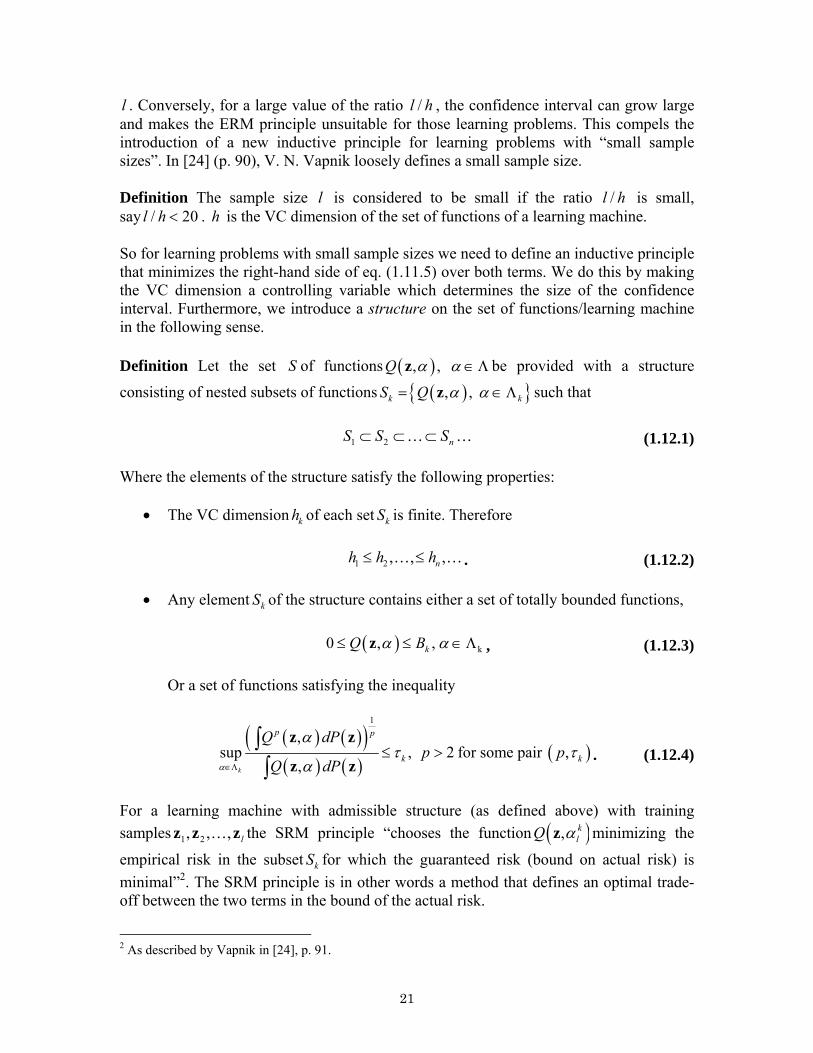
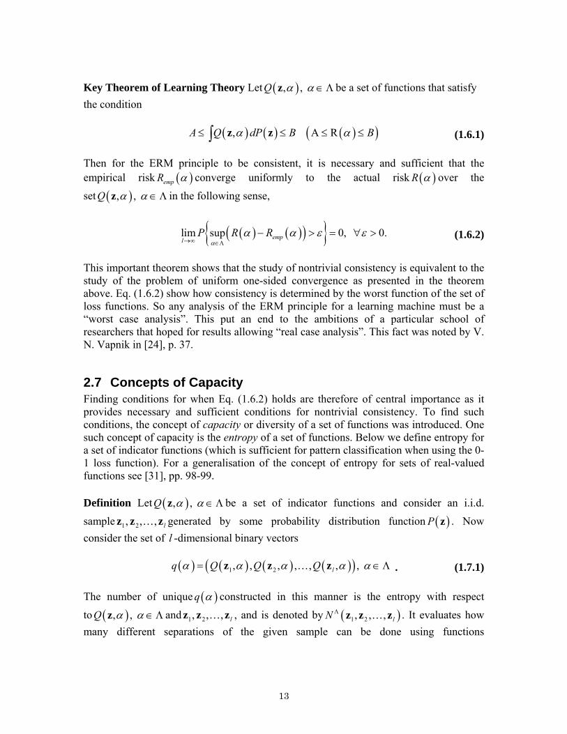
l . Conversely, for a large value of the ratio , the confidence interval can grow large and makes the ERM principle unsuitable for those learning problems. This compels the introduction of a new inductive principle for learning problems with “small sample sizes”. In [24] (p. 90), V. N. Vapnik loosely defines a small sample size.

/l h

Definition The sample size is considered to be small if the ratio is small, say l h . is the VC dimension of the set of functions of a learning machine.

l /l h/ 20< h

So for learning problems with small sample sizes we need to define an inductive principle that minimizes the right-hand side of eq. (1.11.5) over both terms. We do this by making the VC dimension a controlling variable which determines the size of the confidence interval. Furthermore, we introduce a structure on the set of functions/learning machine in the following sense. Definition Let the set of functionsS ( ), , Q α α ∈ Λz be provided with a structure

consisting of nested subsets of functions ( ){ }, , k kS Q α α= ∈ Λz such that (1.12.1) 1 2 nS S S⊂ ⊂ ⊂… … Where the elements of the structure satisfy the following properties:

• The VC dimension of each set is finite. Therefore kh kS

1 2 , , ,nh h h≤ ≤… … . (1.12.2)

• Any element of the structure contains either a set of totally bounded functions, kS

( ) k0 , , kQ Bα α≤ ≤ ∈z Λ , (1.12.3) Or a set of functions satisfying the inequality

( ) ( )( )( ) ( )

(

1

,sup , 2 for some pair ,

,k

p p

k k

Q dPp

Q dPα

α)pτ τ

α∈Λ≤ >∫

∫z z

z z. (1.12.4)

For a learning machine with admissible structure (as defined above) with training samples the SRM principle “chooses the function1 2, , , lz z z… ( ), k

lQ αz minimizing the

empirical risk in the subset for which the guaranteed risk (bound on actual risk) is minimal”

kS2. The SRM principle is in other words a method that defines an optimal trade-

off between the two terms in the bound of the actual risk.

2 As described by Vapnik in [24], p. 91.

21

Figure 6. From eq. (1.10.2) we know that the actual risk is the sum of the confidence interval and the empirical risk. The confidence interval is controlled by the VC dimension of the elements in the structure.

denotes the VC dimension of the element of the structure that provides and optimal trade-off between the empirical risk and confidence interval.

*h

There are two constructive approaches on which learning machines that use the SRM principle are based. In the first approach one determines a set of admissible functions during the design phase of the learning method. This set of functions has to be chosen appropriately so that it gives a reasonable trade-off between the empirical risk and confidence interval for its elements. The VC dimension of this set of functions will fix the confidence interval. With a fixed confidence interval the learning machine then minimizes the empirical risk with respect to the set of function. Neural networks use this approach to SRM. In the second approach the empirical risk is fixed (near zero) and the learning machine minimizes the confidence interval with respect to elements (sets of functions) of the admissible structure. This second approach is applied in support vector machines.

22

3 Support Vector Machines This section aims to give an introduction to the theory of support vector machines (SVMs)3, a methodology in the discipline of soft computing that can be used for classification (SVMC), regression (SVMR) and density estimation learning problems. Due to the context in which this is written (thesis concerning classification of transient states at NPPs), it will only describe SVMs from the viewpoint of pattern recognition (classification). However, using a modified algorithm to what is described below SVM is applicable to learning problems of regression. It may be interesting to point out that it has been shown that SVMC can be seen as a special case of SVMR ([32]). The main mathematical foundation that the theory of SVMs stands on includes fields such as linear algebra, nonlinear optimization (more specifically convex quadratic programmes), functional analysis and statistical learning theory (SLT). The text below assumes some familiarity with each of these fields except for SLT, for which an introductory text is provided in section 2.

3.1 The Linear Separable Case Imagine a linearly separable learning problem with a training set ( ) ( ) ( )( )1 1 2 2, , , , , , n

l lS Y= ⊂x y x y x y… × where can be one of two classes (binary classification). A learning problem is said to be linearly separable if the classes are sufficiently apart from each other so that a single hyperplane can separate them. Let

Y

{ }1,1Y = − , these values representing the labels of the classes and are preferred in the SVM algorithm to for instance { }0,1Y = as it allows a more compact mathematical formulation. By our assumption of linear separability we know that some hyperplane ( ), , , , nf b b b= ⋅ + ∈ ∈w x w x w will separate the two classes that our input points can belong to. Once such a hyperplane has been identified with the help of the training set, the class of other input points can be found by determining what side of the decision boundary the point lies on. The decision boundary is simply the intersection between the input space and a hyperplane, i.e. 0b⋅ + =w x . However, as Figure 7 illustrates any linearly separable learning problem will have more than one separating hyperplane. The choice of a separating hyperplane will affect the generalisation performance of the classifier (learning machine) and we are left with the important decision of choosing a method that selects a hyperplane that maximizes the classifiers generalisation ability.

3 The text on SVMs is loosely based on [33]-[36].

23

Figure 7 – A linearly separable learning problem in has more than one separating hyperplane and hence more than one decision boundary. Points represented as white circles belong to one class while black circles represent the second class. Support vectors have an additional circle encompassing them.

2

Let and be the shortest distances between the separating hyperplane for the closest points of each class in the training set. Training points from each class that satisfy these shortest distances from the separating hyperplane are referred to as support vectors. The margin of the separating hyperplane with respect to some training set we define as . It has been proven that the separating hyperplane with maximal margin displays best generalisation ability. For this reason we are interested in finding such a hyperplane and this type of learning machine is sometimes referred to as a maximal margin classifier.

1d 1d−

1d d−+ 1

In formulating a mathematical expression for the margin of a hyperplane we use the fact that each hyperplane , b+w x defines the discriminant function

as ( ) ( )f sign b= ⋅x w x + . Input points that return negative values of belong to one class while positive values assign the input point to the other class. With this discriminant function it easy to see that hyperplanes

( )f x

( ) , for any k b k⋅ +w x ∈

)

define the same discriminant function. This allows and to be scaled arbitrarily without changing the output of the discriminant (also called decision) function. Choose ( such

that

w b,bw

1, for all support vectors SV SVb⋅ + =w x x . This representation of the optimal hyperplane is called the optimal canonical hyperplane. The canonical form implies

( )1 if 1

for all ,1 if 1

i ii i

i i

b yy S

b y⋅ + ≥ =

∈⋅ + ≤ − = −w x

xw x

which is equivalent to the more compact notation

24

( ) 1, 1, , .i iy b i⋅ + ≥ =w x … l

The margin of the hyperplane can now be expressed in terms of by means of two additional hyperplanes

w1 : 1H b⋅ = −w x and 2 : 1H b⋅ = − −w x , on which all support

vectors lie as illustrated in Figure 7. Using the fact that , and our separating hyperplane are perpendicular and that their perpendicular distances from the origin are,

1H 2H

1 b−

w,

1 b− −w

andbw

respectively,

we get 1 11d d−= =w

and that the margin is 2w

.

In the paragraph above we have shown that the process of finding the separating hyperplane with largest margin is equivalent to finding a separating hyperplane in canonical form with minimal Euclidian norm of . This is suitably expressed as the following nonlinear optimization problem,

w

( )

2

,

1min2

subject to 1 0, 1, .b

i iy b i⋅ + − ≥ =

ww

x w …l (2.1.1)

The Lagrangian formulation of this optimization problem makes it easier to solve and in our case the Lagrangian is as following:

( ) ( )2

1

1, ,2subject to 0, .

l l

i i i ii

i

L b y b

i1i

α α α

α=

= − ⋅ + +

≥ ∀=

∑ ∑w w x w (2.1.2)

Sufficient conditions for optimality for any given nonlinear optimisation problem are given by the saddle point theorem which for our problem states that any point is a local optimum if it satisfies ( , )opt optbw

( ) ( ) ( )

( ) (,0

, , , , , ,

, , max min , , .

opt opt opt opt opt opt

opt opt opt

b

L b L b L b

L b L bα

α α

α α≥

≤ ≤

⇔

=w

w w w

w w )

α

(2.1.3)

25

Due to the saddle point theorem we can reformulate the original problem into the Lagrangian dual problem (also called the Wolfe dual) by maximizing ( ), ,L b αw with respect toα subject to the constraints that the gradient with respect to w andb vanish,

( )

( )

,, , 0, 1,

0., , 0

v i i i v i i ii iv

i ii iii

L b w y x v n yw

yL b yb

δ α α αδδ αα αδ

⎧ ⎧= − = = =⎪ ⎪⎪ ⎪⇒⎨ ⎨⎪ ⎪ == − =⎪ ⎪⎩⎩

∑ ∑

∑∑

w w x

w

… (2.1.4)

Being equality constraints they can be substituted into the objective function ( ), ,L b αw giving,

0 ,

1max .2i i j i j i

i jy y

αα α α

≥−∑ ∑ x x j⋅

x

(2.1.5)

The solution of this final formulation of the optimisation problem is then substituted into

giving a partial solution to eq. (2.1.1). Let us now study the Karush-Kuhn-

Tucker complementary condition which our solution must satisfy:

i i ii

yα= ∑w

( )( )1 0, i i iy bα .i⋅ + − = ∀w x (2.1.6) Firstly, note that for all that are not support vectors,ix ( ) 1i iy b⋅ + >w x implying 0iα = . This in turn means that

. (2.1.7) 1

where is the number of support vectors ( )svN

i i i i i i sv ii i

y y Nα α=

= =∑ ∑w x s s

This has beneficial practical implications as support vectors are scarce in training sets. In an extensive study of a digit recognition problem ([38] and [39]) described by V. N. Vapnik in [24] the support vectors amounted to between 3-5% of the total number of training points. This property reduced the time it takes to train a SVM classifier as only the support vectors are used in calculations. This also means that the SVM methodology scales well to large sets of training points. Secondly, the complementary condition allows us to calculateb using any for which is a support vector. In practise this is normally done by taking the average of all such equations. We have thus found the maximal margin hyperplane

i ix

0b⋅ + =w x

26

and new input points can be classified into one of two classes with the resulting decision function

( ) ( )1

sgn sgn .svN

i i ii

f b yα=

⎛ ⎞= ⋅ + = ⋅ +⎜

⎝ ⎠∑x w x s x b ⎟

l

(2.1.8)

It is important to note that our solution is global due to the convexity of the optimisation problem considered. This is a considerable advantage over for instance neural networks for which only local solutions are guaranteed.

3.2 The Linear Non-separable Case For training sets that are linearly separable but have imperfect separation due to for instance noise we introduce positive slack variables , 1, ,i iξ = … so that

( )

1 for 1

1 for 1

1 , .

i i i

i i i

i i i

b y

b y

y b

ξ

ξ

ξ i

⋅ − ≥ − =

⋅ − ≤ − − = −

⇔

⋅ − ≥ − ∀

w x

w x

w x

(2.2.1)

These slack variables correspond to penalty terms associated with each training point. The further a training point strays from the hyperplane on which the support vectors of the same class lie on, the larger a penalty it incurs (see Figure 8).

Figure 8. The introduction of slack variables , 1, ,i i lξ = … provide a formulation for learning problems with linear underlying dependencies but imperfectly separated training data due to noise, etc.

27

Taking the slack variables into consideration, the optimization problem now instead becomes,

( )

2

, , 1

1min2

subject to 1 0, 1, ,

0, 1, ,

i

l

ib i

i i i

i

C

y b i

i l

ξξ

ξ

ξ

=

+

⋅ + + − ≥ =

≥ =

∑ww

w x …

…

l (2.2.2)

Following the steps in subsection 3.1 we find that neither the slack variables nor their Lagrange multipliers appear in the Lagrangian dual problem (compare to eq. (2.1.5)),

,

1max2

subject to0 .

i i j i j ii i j

i

y y

C

αα α α

α

j− ⋅

≤ ≤

∑ ∑ x x (2.2.3)

Again the solution is

1

where is the number of support vectors ( )svN

i i i i i i sv ii i

y y Nα α=

= =∑ ∑w x s s

giving decision function

( )1

sgn .svN

i i ii

f y bα=

⎛ ⎞= ⋅⎜ ⎟

⎝ ⎠∑x s +x

3.3 The Non-Linear Case For nonlinear training sets the input points are mapped by some transformation into a high (possibly infinite) dimensional Euclidian feature space

( )Φ ⋅H in which the training set

become linearly separable. In this feature space our existing technique for linearly separable training sets can be applied thanks to what is often referred to as the “kernel trick”. Eq. (2.2.3) now becomes

( ) ( )

1 ,

1max2

subject to 0 .

l

i i j i j ii i j

i

y y

C

αα α α

α=

− Φ ⋅Φ

≤ ≤

∑ ∑ x x j (2.3.1)

and similarly to eq. (2.1.8) our new decision function is

( ) ( ) ( )1

sgnSVN

i i ii

f yα=

⎛ ⎞= Φ ⋅Φ⎜

⎝ ⎠∑x s b+ ⎟x . (2.3.2)

28

The problem here is that the calculation of dot products in high dimensional spaces is, if not impossible, a highly cumbersome task. This step is omitted by the introduction of a kernel function ( ) ( ) ( ),i j i jK = Φ ⋅Φx x x x which calculates the dot products implicitly

using the original input points. Note that the explicit formulation of the transformation is unnecessary and is often unknown for kernel functions. This idea is simple enough, but how do we know which functions can be used as kernel functions, i.e. return dot products in some high dimensional Euclidian space?

( )Φ ⋅

This is guaranteed by Mercer’s theorem: Theorem There exists a mapping Φ and an expansion ( ) ( ) ( ), ,i j i jK = Φ ⋅Φx x x x if and only if, for any ( )g x such that

( )2 is finite,g d∫ x x then ( ) ( ) ( ), 0i j i j i jK g g d d ≥∫∫ x x x x x x . By substitution of the kernel function in eq. (2.3.2) we finally get

( ) ( )1

sgn ,SVN

i i ii

f y K bα=

⎛ ⎞= +⎜

⎝ ⎠∑x s ⎟x . (2.3.3)

29

Figure 9. The original input space is mapped onto a high-dimensional Euclidian feature space in which the training set is linearly separable.

The following are well-known examples of kernel functions,

• Polynomial Kernel: ( ) ( ), 1p

i j i jK p, = ⋅ + ∈x x x x

• Radial Basis Function Kernel: ( ) ( )2 2, exp / 2 , i j i jK γ γ= − − ∈x x x x

• Sigmoid Kernel: ( ) ( ), tanh , ,i j i jK γ δ δ γ= ⋅ − ∈x x x x

Note that unlike polynomial and radial basis function kernels, sigmoid kernels only satisfy Mercer’s conditions for certain values of parametersδ ∈ andγ ∈ . In the formulation of SVM classifiers above it is clear that they are intrinsically binary classifiers, i.e. they can tackle pattern recognition problems where the samples can belong to one of two classes. Naturally, many pattern recognition problems have input points that can belong to more than two classes. So far, researchers have been unable to generalize the SVM classifier formulation to intrinsically support multi-class classification. Instead, a variety of methods exist that generally break down a multi-class problem into several binary problems. One popular technique, the “One vs. One classifier” proposed by J. Friedmann in [40], creates binary classifiers for each combination of classes possible. Unseen examples are then classified to the class that performs best in these binary classifiers. For a comparative study of several multi-class techniques see [41].

30

4 Experiments

4.1 Phase 1 – Manually Generated Data Before applying support vector machines (SVM) to the task of identifying transients from data obtained from a reactor simulator (MAAP [42]), a preparatory experiment was set up with the aim of providing insight to the problem at hand. It was hoped that such an experiment could identify potential pitfalls in the main phase (section 4.2) and give an indication as to how SVM classifiers would perform with real data. This study was set up as a comparison between SVM and neural network (NN) classifiers. In the context of a comparative study of the abovementioned learning machines it was important to identify performance criteria on which comparisons could be made. As these criteria strongly influence the design of the experiment we will first identify these and their underlying motivations. Transient identification at Nuclear Power Plants (NPPs) is a safety-critical process and demands high reliability. In terms of learning methodologies, this translates to finding learning machines that are able to train classifiers with high classification accuracy. Specifically, it is crucial not to misclassify transient signals as non-transient as this may lead to an unacceptable delay in the detection of a severe reactor state. Misclassifications of the second kind can be manually overridden by human operators (after inspection) and therefore, do not pose the same type of threat to reactor operation. Classification accuracy is of outmost importance and is considered as our primary performance criterion. Ideally, the process of transient identification should be conducted on-line. This poses restrictions on the amount of time it should take for a classifier to identify which class (transient or non-transient) a signal belongs to. The second performance criterion is therefore the time taken to classify a given signal.

4.1.1 Structure of Experiment The general structure of the experiment consisted of the following steps (for both methodologies):

1. Generation of training and test set using signal prototypes. Assigning appropriate labels to each element in the sets.

2. Generation and application of noise to both sets described above. 3. Scaling/normalising both sets. 4. Design parameter optimisation. 5. Training classifier with training set. 6. Testing resulting classifiers using training set 7. Collecting results.

These steps were repeated a number of times for given experiment parameters such as size of sets and amount of noise. Each step is elaborated on in the following subsections.

31

See subsection 4.1.8 for a description of what parameter values were used in the experiment.

Generate Sets (1-3)

Figure 10. Flow chart of steps taken in experiment.

4.1.2 Signal Prototypes In this experiment 8 transient and 8 non-transient signal prototypes were “manually” constructed, from which all training and test points are derived. The signal prototypes try to capture general features that appear in real transient and non-transient signals. The prototypes were all generated using Matlab. Signals that didn’t have obvious mathematical representations (particularly for the transient signals) were “sketched” by manual insertion of values to form a plot with approximately desired shape. This plot was initially jagged due to few entry points and was smoothened with Matlab’s inbuilt shape-preserving interpolation function. Finally, these resulting signals were discretized with a sample frequency of 20, 40 and 160.

Train Classifier (5)

Test Classifier (6)

Design (4) Change Design Parameters

Change Noise Level and Set Sizes

Collect Results (7)

32

Arbi

trary

Uni

ts (y

)

time (s) time (s)

Figure 11. Transient Signal Prototypes. The horizontal and vertical axes represent time and value of signal respectively. The sample intervals are equally spaced over time.

Arbi

trary

Uni

ts (y

)

time (s) time (s)

Figure 12. Non-transient signal prototypes.

33

4.1.3 Generation of Training and Test Sets In supervised learning machines, to which both SVM and NN methodologies belong, one set of data points is used to train and one set to test the classifier. Since no set of real data points was available, both training and test set were generated. In the SVM test runs, the training set roughly constituted 80% of the total number of generated points, and the test set the remaining 20%. In the NN case, a different ratio was employed due to a method used called early stopping. Early stopping requires an additional set called the validation set. A more detailed description of this appears in subsection 4.1.7. The training, test and validation set roughly constituted 50%, 25% and 25% of the total number of input points respectively. In supervised learning best results are obtained when the training set is a good representative of the set of all possible points. In other words, the data points in the training set should be spread out evenly in the input space so as to capture as much of the underlying nature of the input space as possible. This experiment only dealt with representative training set. In practical terms this means that each set consisted of an equal amount of transient and non-transient signals. Furthermore, for each type of signal, the set of such signals was generated by simply cycling through the prototypes of the corresponding type, adding Gaussian noise and appending the resulting signal values to the training set as an input point. This way each signal prototype would roughly have the same proportion of signals in the training set. The training set is generated in an identical manner, giving the training set good representative capabilities. However, it is important to note that in real-life applications it is generally hard to select/find representative training sets. It would therefore be good, at some future point, to extend the current experiment to non-representative training sets.

4.1.4 Addition of Gaussian Noise The methodologies were compared for various levels of noise in the training and test sets. For each run of the experiment both sets were given the same level of noise, as expected in real-life data sets. When implementing the ability to set the level of noise, a noise coefficientα was introduced. This constant should be interpreted as the highest percentage we allow the noise to have in relation to the average of the absolute values of all values that make up the signal. So, for a set of points that define a signal that we represent in vector notation ( 1, , n )x x=x … , noise is added in the following manner:

1

1

1where is an instance of the random variable 0, .3

l

new i oldi

x x y xl

y Y

α=

⎛ ⎞= ⋅ ⋅ +⎜ ⎟⎝ ⎠

⎛ ⎞⎜ ⎟⎝ ⎠

∑

∼ N (3.1.1)

34

Note that the limit imposed byα is not strict as only 99.7% of instances of fall within three standard deviations of the mean.Y is a random variable with zero mean and a standard deviation of 1/3.

y

α = 0.0 α = 0.1

Arbi

trary

Uni

ts (y

)

α = 0.4 α = 0.9

time (s) time (s)

Figure 13. A transient signal prototype with four different levels of the noise coefficientα .

4.1.5 Normalising Training and Test Sets Before a training set can be passed on to train a classifier many learning machine methodologies rely on the data to be normalised. This is done to prevent input points with high values from dominating in the learning process over points with low values. Normalising also alleviates various numerical complications that certain learning machines are susceptible to. Although data were chosen with this in mind it was still deemed good practise to let the data undergo normalisation. Hence, all input points of the training set were scaled to lie in the interval[ ]1,1− . Target values were ignored as they already met this requirement. For the SVM classifier, non-transient signals were assigned the target value 1 while transient signals were assigned the value -1. For NN classifiers, non-transient signal were assigned to 0 and transient to 1. Based on the minimum and maximum values of the training set the points in the test set could then also be normalised using the following formula,

35

( ),min

,max ,min

2 old trainnew

train train

p pp

p p−

1= −−

(3.1.2)

where and are minimum and maximum values of the training set in the dimension to which

,mintrainp ,maxtrainp

oldp belongs to.

4.1.6 Implementation of SVM Methodology Training and testing of the SVM classifier was conducted using an existing C library, SVMLib [43]. This library implements C-SVC (support vector classification) using implementation techniques such as Sequential Minimal Optimization (SMO) [44]. Python scripts were used to cross-validate, generate and pre-process the signals as well call SVMLib’s binary executables for the various test runs. The SVM approach requires the choosing of a kernel function. These experiments used the Radial Basis Function (RBF) kernel as recommended by the authors of SVMLib [45]. RBF kernels are generally considered good to start with as they present few numerical difficulties, only use one hyper-parameter (γ ) and in most cases generalise well. RBF kernels have the following form:

( ) ( )2, exp ,i j i jK x x x xγ γ 0.= − − > (3.1.3)

The only other parameter (C ) that needs to be specified stems from the optimisation problem which C-Support Vector Classification is often given in:

( )( ), , 1

1min2

subject to 1 ,

0.

lT

iw b i

Ti i

i

w w C

y w x b

ξξ

iφ ξ

ξ

=

+

+ ≥ −

≥

∑

(3.1.4)

Optimising the classifier with respect to these parameters was achieved by using 5-fold, grid-search cross-validation. Cross-validation is a simple yet efficient re-usage of sample data often employed when optimising parameters of learning machines. In m-fold cross-validation the training set is randomly divided into m disjoint sets of equal size. A classifier is trained for each of these sets each time with a different sets used as the validation set. The estimated performance is the mean of the m errors. Grid-search refers to a technique that performs cross-validation on pre-specified parameter pairs ( ),C γ . The advantages of this technique are that it is simple and exhaustive while the main drawback is that it is computationally expensive. This

36

experiment (as recommended by the authors of [45]) used exponentially growing sequences of the parameter values, more specifically

. 5 3 1 3

15 13 11 3

2 , 2 , 2 , , 22 , 2 , 2 , , 2

Cγ

− − −

− − −

=

=

……

This is a rather coarse grid-search step size and may be improved by repeating the procedure with a smaller step size within the grid that performed best during the first iteration. This was not performed in this experiment as initial results were considered good.

4.1.7 Implementation of NN Methodology The methodology of neural networks entails a plethora of different architectures and algorithms whose performances vary with respect to the learning problem. Two main sources were used to identify the architectures/learning algorithms best suited for our particular problem - “The Neural Network FAQ” (NNFAQ) [46] and Matlab’s Neural Network Toolbox Documentation (MNNTD) [47]. These sources (especially [46]) summarize information from various papers, articles, etc. All coming references in the subsection will point to one of the two main sources and not the work that some of the information may originate from. First off all, an appropriate type of neural network was sought. Two were identified as potential candidates – feed-forward back-propagation (FFBP) multi-layer networks and radial basis function (RBF) networks. FFBP networks were chosen instead of RBF networks. The main reasons for this choice are that 1) existing related literature predominately use FFBP networks. 2) RBF networks work best when a large training set is available. This experiment uses a variety of training sets of different sizes (many small) raising some concern. Note however that these reasons are of minor significance and that the choice was rather arbitrary. Standard back-propagation is a gradient descent algorithm and is used as the FFBP network’s learning rule. There are a number of variations of the basic algorithm and their suitability depends on the learning problem. MNNTD have a speed and memory comparison of some of these learning rules on a set of learning problems (some simple “toy” problems, others real-life applications). In this comparison two of them distinguished themselves from the rest for pattern recognition problems, namely the resilient back-propagation and scaled conjugate gradient algorithms. The following is a summary of relevant discoveries in MNNTD’s comparative study. The resilient back-propagation algorithm converged fastest on all pattern recognition problems. This is reasonable as the algorithm was designed to overcome some of the difficulties present in pattern recognition problems. However, its performance degrades as the error goal is reduced. Memory requirements are relatively small when compared to the other variations of the back-propagation learning rule. Matlab implements this algorithm in the trainrp function. From here on the resilient back-propagation algorithm will be referred to as trainrp.

37

The scaled conjugate gradient algorithm performed well for a variety of problems (regression and pattern recognition), especially for networks with a large number of weights. It is almost as fast as the prior algorithm, but its performance does not degrade as fast when the error goal is reduced. Memory requirements are modest and Matlab implements this algorithm in the trainscg function. The neural network classifier’s in this experiment use the trainrp learning rule. The main reason in our choice of trainrp over trainscg was its fast convergence. Also, the fact that trainscg works best for large number of weights raised concern. This would severely increase the training time - a factor which ended up prevented a rigorous comparative study of NN and SVM classifiers (even when only using trainrp). This was due to an incorrect experimental set-up and will be elaborated on in section 4.1.10. Next, it was important to complement the chosen algorithms with some technique that prevents overfitting. Overfitting is a term used to describe when the learning algorithm adapts its weights in too close accordance with the input points of the training set. This leads to good performance on the training set but in most cases poor generalisation ability. In statistical terms this corresponds to low bias but high variance. MNNTD discusses and has implemented two such techniques – regularisation and early stopping. Furthermore, it mentions that early stopping usually works well for both trainrp and trainscg algorithms. With this in mind, trainrp was used in conjunction with early stopping. However, it should be noted that regularisation is in many cases better than early stopping, especially for cases where the training set is small. In early stopping, the available set of input points is divided into three subsets – a training, validation and test set. In this experiment, the sets account for approximately 50%, 25% and 25% of the total number of input points respectively. As usual, the training set is used for computing the gradient and updating the weights and biases. The error on the validation set is monitored throughout training. At some point in training, the neural network will typically start overfitting which is picked up by the network in the error of the validation set. When this happens, training is stopped, weights and biases are returned to where the validation error was smallest and testing can ensue on the resulting network. In early stopping, it is important that the validation set is representative of the underlying input space. Also essential for both the early stopping and regularisation techniques is to train the network from many different initial conditions as training can fail in certain runs. The last yet an important features to determine in a neural network is its topology, i.e. number of hidden layers and number of neurons present in each layer. The topology of the network is crucial to a network’s performance and the optimal choice may according to NNFAQ depend on the following factors:

• the numbers of input and output units • the number of training cases • the amount of noise in the targets

38

• the complexity of the function or classification to be learned • the architecture • the type of hidden unit activation function • the training algorithm • regularization

Judging by the long list of factors, the process of choosing an optimal topology is non-trivial. Moreover, given the multitude of training sets (on which to model a network for) in this experiment it was necessary to automate this process. In [48], the authors identify three main types of automated parameter design4 (also known as Design of Experiment (DoE)) – one-factor-at-a-time, full factorial and fractional factorial. The first method is crude and rarely gives an accurate estimation of the optimal parameter design. The full factorial method on the other hand evaluates every combination of parameter values making it exhaustive yet time-consuming. Fractional factorial methods use wise selection of parameter sets to give comparable performance to full factorial methods in a fraction of the time. They do however take a longer time to implement. This experiment uses the full factorial method in the design of parameters.

Along with the topology of a network, the parameters specific to the training algorithm make up the so called design parameters. This experiment assumed that Matlab’s default values of algorithm-specific parameters were close to optimal, leaving only the topology of the network to be determined. For this purpose the full factorial method was used trying topologies with one and two hidden layers. MNNTD states that it is important to have a large number of hidden units when using early stopping, thus avoiding bad local optima. Furthermore MNNTD asserts that there does not seem to be an upper bound on the number of hidden units (that may provide an optimum); but it continues by saying that there is seemly no advantage in using more hidden units than available training points. For this reason, topologies were tried where the total number of hidden units ranged from 2 to the number of training points (for both one and two hidden layers).5

An improvement of the full factorial method used above is the fractional factorial method and would be considered in an eventual continuation of this experiment. It would be advisable to use some form of the fractional factorial method for any complex real-life application of neural networks. The Taguchi Design of Experiments [49] coupled with Analysis of Variance (ANOVA) is a popular example of the abovementioned method.

The number of neurons in the input and output layer of the network are determined by the dimensionality of the input space and dimensionality of the expected target space respectively. As the signals are discretized into 20, 40 or 160 points and no feature selection was performed the points determine the number of neurons in the input layer. The task of transient identification is a case of binary classification which we have

4 Evolutionary computing, complex structures and complex learning rules are identified as additional methods for automated parameter design in [50]. 5In training with the larger sets of this experiment a hard-limit was imposed on the number of hidden layers (40) and the number of hidden layers (1). This was done due to unacceptable training times of classifiers based on large training sets.

39

chosen to represent by a one neuron output layer using the log-sigmoid transfer function. All hidden layers use the tan-sigmoid transfer function. The input vectors are presented to the network concurrently and in batches (which is most efficient).

4.1.8 Test Runs The process described above is repeated for numerous different training and test set pairs. The parameters that vary between each test run are

1. The sample frequency of the signals. 2. The noise level coefficientα . 3. The size of the training, validation6 and test sets.

For each set of specified parameters, the generation of signals and training/testing of classifiers with these signals was repeated 100 times. This was done to provide a more accurate picture of the NN and SVM classifier performances, and is especially important for classifiers trained with small sample sizes. The results shown in section 4.1.9 are the average values attained from these 100 repetitions. In retrospect, this experimental setup was inappropriate due to the computationally expensive nature of the neural network classifiers, specifically in parameter design. The large number of parameters and repetitions for each parameter set led to unreasonable training times. For this reason, a crippling compromise was but in place – the training set sizes for the NN method was limited to 100 training points. Furthermore, although an additional discretization (160 points) was prepared it was abandoned after learning that NN classifiers in practise never exceeded approx. 40 input neurons. SVM classifiers have a much higher limit on the dimensionality of the input space. For a fair comparison of higher dimensions it would be necessary to apply some form of feature selection technique that could reduce this number. The parameters are assigned the following values

1. Sample frequency – 20 and 40. 2. Noise level coefficient – 0.0, 0.05, 0.1, 0.2, 0.3, 0.4, 0.5 and 0.6. 3. Size of training set – 20, 40, 60, 80, 100, (250, 500 and 750)7.

The size of the test and validation sets is determined by the size of the training set. When using the SVM classifier the test set constitutes approximately 20% of the total number of input points. In the NN case, both the validation and test sets stand for approximately 25% of the total number of input points. All of the runs were performed under Windows XP on an Athlon XP 2800+, 2.07 Ghz with 1.0 Gb of RAM.

6 The validation set only applies to neural network methodology as it is used in early stopping. 7 These last sizes of the training set were only tested for SVM classifiers.

40

4.1.9 Results

20 30 40 50 60 70 80 90 10075

80

85

90

95

100

Number of Training Points

Ave

rage

Cla

ssifi

catio

n A

ccur

acy

(%)

Phase 2: SVM Classifiers (s.f. = 20)

α = 0.1α = 0.2α = 0.3α = 0.4α = 0.5α = 0.6

20 30 40 50 60 70 80 90 10075

80

85

90

95

100

Number of Training Points

Ave

rage

Cla

ssifi

catio

n A

ccur

acy

(%)

Phase 1: NN Classifiers (s.f. = 20)

α = 0.1α = 0.2α = 0.3α = 0.4α = 0.5α = 0.6

41

20 30 40 50 60 70 80 90 10075

80

85

90

95

100

Number of Training Points

Ave

rage

Cla

ssifi

catio

n A

ccur

acy

(%)

Phase 2: SVM Classifiers (s.f. = 40)

α = 0.1α = 0.2α = 0.3α = 0.4α = 0.5α = 0.6

20 30 40 50 60 70 80 90 10075

80

85

90

95

100

Number of Training Points

Ave

rage

Cla

ssifi

catio

n A

ccur

acy

(%)

Phase 1: NN Classifiers (s.f. = 40)

α = 0.1α = 0.2α = 0.3α = 0.4α = 0.5α = 0.6

42

250 300 350 400 450 500 550 600 650 700 75099

99.1

99.2

99.3

99.4

99.5

99.6

99.7

99.8

99.9

100

Number of Training Points

Ave

rage

Cla

ssifi

catio

n A

ccur

acy

(%)

Phase 2: SVM Classifiers (s.f. = 20)

α = 0.1α = 0.2α = 0.3α = 0.4α = 0.5α = 0.6

250 300 350 400 450 500 550 600 650 700 75099

99.1

99.2

99.3

99.4

99.5

99.6

99.7

99.8

99.9

100

Number of Training Points

Ave

rage

Cla

ssifi

catio

n A

ccur

acy

(%)

Phase 2: SVM Classifiers (s.f. = 40)

α = 0.1α = 0.2α = 0.3α = 0.4α = 0.5α = 0.6

Preliminary results for the time taken to test new input points with classifiers of each kind showed that both methods do so well within limits dictated by the requirements of on-line monitoring. For this reason, our second performance criterion will have little bearing on our comparative study and have thus been omitted.

43

4.1.10 Conclusion The layout of this phase was designed on the basis of prior practical experience with SVM classifiers. The (in many respects) similar nature of SVM and NN classifiers led to overly optimistic assumptions about steps necessary in the optimal training of latter. The multitude of trials for the already large number of parameter sets presented overbearing computational demands with respect to the time frame, equipment and techniques used in the design of parameters. This led to an inappropriate design of the experiment that forced a simplified implementation of the NN classifiers whose performance can probably be improved on. The results are therefore probably biased in favour of SVM classifiers. For this reason, the comparative study of SVM and NN classifiers can be viewed as a partial failure. The results in section 4.1.9 show how SVM classifiers outperformed the NN classifiers for most of the chosen parameter sets and this for both sample frequencies (20 and 40). Only for scenarios with the smallest number of training points (20) and high levels of noise did NNs score better than SVMs. It is interesting to note that SVM classifiers consistently converged to a maximal classification rate as the number of training points increased. NN classifiers however had no visible change in performance relative to the size of the training set. This could be due to the hard maximum limit imposed on the number of hidden neurons. One major difference (of practical importance) between the two types of learning machines is the number of unknown parameters. These parameters have to be determined experimentally as no significant theoretical results bind these parameters to the performance of the classifier. These parameters do however have a significant effect on the performance and an appropriate choice of these is crucial. SVM classifiers generally have no more than three parameters and these stem from the objective function of the nonlinear optimization programme and kernel function. NN classifiers have a far greater number of parameters that stem from the NN learning machine’s learning rule, the topology of the network and technique that prevents overfitting (such as regularization). The small number of parameters in SVMs makes simple “brute force” techniques such as grid-search viable in cases where this would be incredibly impractical for NNs. Another advantage of SVMs is their ability to deal with far greater dimensions of the input space. In reviewed literature, the dimension of the input space of NN learning machines rarely went above 40. Instead, various techniques of feature selection such as principal component analysis (PCA) are employed to reduce the input space into a feature space of lower dimension. For many learning problems, SVMs will be able to handle the original input space and thus does not lose any information in the process of feature selection. How large the input space’s dimension can be in practise has not been determined in this experiment but reviewed articles suggest an input dimension of at least 300.

44

4.2 Phase 2 – MAAP Simulated Data In the second practical phase of this thesis, SVM classifiers were investigated on signals simulated by a program called Modular Accident Analysis Program (MAAP). This phase is not a comparative study between SVM and NN classifier like in Phase 1, but rather tries to determine how suitable SVM classification is for sensor-based transient identification at nuclear power plants. Phase 1 showed that the time it takes to classify new input points was so low that it was unlikely to be a limiting factor in most real-time/on-line monitoring systems. Therefore, the only performance criteria looked at in this phase is the generalization ability of the SVM classifiers.

4.2.1 The MAAP Signals

Program Simulating Operation of Nuclear Power Plant Modular Accident Analysis Program (MAAP) was developed by Fauske & Associantes, Inc. (FAI) to facilitate the nuclear industry with analytic assessment methods of responses to different events that might occur in light water nuclear power plants (LWR). It comes equipped with physical models of all processes that have importance in the event of an emergency that leads to core damage. Below is a list of the main processes that are modelled:

• Heat flow. • Liquid flow. • Handling and liberation of radioactive products. • System operation. • Operator’s behaviour. • Vaporisation. • Fuel temperature rise. • Oxidation and damage of can.

Furthermore, MAAP can simulate constructions of a number of cores of which these are selection:

• Typical pressurized water reactor (PWR) core. • Typical boiling water reactor (BWR) core. • Core of VVER reactors.

This thesis will limit itself to signals generated for different states that one might expect to find in boiling water reactors (BWR) (in accordance with M. Bednarski [1]).

45

Accident Sequences Each set of signals generated are done so for specific accident sequences that might occur at the power plant. The sequences are divided into two groups where one is used for training and the other for testing. A sequence is characterized by a combination of possible states for four available events:

• Pipe failure (Water) – with states: small, medium and large. • Pipe failure (Steam) – small, medium and large. • Leakage between drywell and wetwell – small, medium and large. • Operation level of safety systems – none ( 0% ) and full ( 100 % ).

In each of the above events, the small, medium and large states correspond to 1%, 50% and maximum leak area respectively. Water and steam pipe failures were deemed mutually exclusive events which produces a total of ( )1 1 1 2 22 3 3 2 2 3 36⋅ ⋅ ⋅ = ⋅ = training sequences. M. Bednarski listed all 36 training sequences in Table 1. The 12 testing sequences are slight variations of some of the training sequences and are presented in Table 2. M. Bednarski selected these sequences on the basis of:

• Probability Safety Analysis (PSA) [51]. • Discussion with specialists in the field of PSA analyses in Forsmark power plant. • Safety criteria. • Time-consumption criteria of calculating simulations.

Finally, note that “…each sequence is accompanied by the loss of AC power causing inaccessibility of the recirculation system and cooling water supply system” [1].

46

Table 1. Training sequences.

Sequence Type of pipe

Size of pipe failure [m2]

Area of leakage between drywell and wetwell [m2]

Operation level of safety systems

Sequence 1 water 0,0471 0,01413 100% Sequence 2 water 0,02355 0,01413 100% Sequence 3 water 0,00471 0,01413 100% Sequence 4 water 0,0471 0,01413 0% Sequence 5 water 0,02355 0,01413 0% Sequence 6 water 0,00471 0,01413 0% Sequence 7 steam 0,0735 0,01413 100% Sequence 8 steam 0,03675 0,01413 100% Sequence 9 steam 0,00735 0,01413 100% Sequence 10 steam 0,0735 0,01413 0% Sequence 11 steam 0,03675 0,01413 0% Sequence 12 steam 0,00735 0,01413 0% Sequence 13 water 0,0471 0,07065 100% Sequence 14 water 0,02355 0,07065 100% Sequence 15 water 0,00471 0,07065 100% Sequence 16 water 0,0471 0,07065 0% Sequence 17 water 0,02355 0,07065 0% Sequence 18 water 0,00471 0,07065 0% Sequence 19 steam 0,0735 0,07065 100% Sequence 20 steam 0,03675 0,07065 100% Sequence 21 steam 0,00735 0,07065 100% Sequence 22 steam 0,0735 0,07065 0% Sequence 23 steam 0,03675 0,07065 0% Sequence 24 steam 0,00735 0,07065 0% Sequence 25 water 0,0471 0,1413 100% Sequence 26 water 0,02355 0,1413 100% Sequence 27 water 0,00471 0,1413 100% Sequence 28 water 0,0471 0,1413 0% Sequence 29 water 0,02355 0,1413 0% Sequence 30 water 0,00471 0,1413 0% Sequence 31 steam 0,0735 0,1413 100% Sequence 32 steam 0,03675 0,1413 100%

47

Sequence 33 steam 0,00735 0,1413 100% Sequence 34 steam 0,0735 0,1413 0% Sequence 35 steam 0,03675 0,1413 0% Sequence 36 steam 0,00735 0,1413 0%

Table 2. Test sequences.

Sequence Type of pipe

Size of pipe failure [m2]

Area of leakage between drywell and wetwell [m2]

Operation level of safety systems

Sequence t1 water 0,03768 m2 0,01413 100% Sequence t2 water 0,03768 m2 0,01413 0% Sequence t3 steam 0,0588 m2 0,01413 100% Sequence t4 steam 0,0588 m2 0,01413 0% Sequence t5 water 0,0471m2 0,04239 100% Sequence t6 water 0,0471m2 0,04239 0% Sequence t7 steam 0,0735m2 0,04239 100% Sequence t8 steam 0,0735m2 0,04239 0% Sequence t9 water 0,0471m2 0,01413 50%****

Sequence t10 water 0,00471 m2 0,01413 50%**** Sequence t11 steam 0,0735m2 0,01413 50%**** Sequence t12 steam 0,00735 m2 0,01413 50%****

**** this means that in each safety system 2 pumps of 4 will be switched off.

48

Table 3. Representative overview of the simulated sequences.

Rupture (m2) / Label Leakage (m2) Safety (%)

Water Pipe 0,00471m2 / W1 0,02355m2 / W5

0,04710m2 / W10

0,01413m2 = 1 0,07065m2 = 5 0,14130m2 =10

0% 100%

36 T

rain

ing

Sequ

ence

s

Steam Pipe 0,00735m2 / S1 0,03675m2 / S5 0,07350m2 / S10

0,01413m2 = 1 0,07065m2 = 5 0,14130m2 =10

0% 100%

Water Pipe 0,00471m2 / W1 0,03768m2 / W8 0,04710m2 / W10

0,01413m2 = 1 0,04239m2 = 3

0% 50% 100%

12 T

estin

g Se

quen

ces

Steam Pipe 0,00735m2 / S1 0,05880m2 / S8 0,07350m2 / S10

0,01413m2 = 1 0,04239m2 = 3

0% 50% 100%

Signals Each accident sequence is made of eight simulated signals representing various processes of the reactor containment. M. Bednarski chose them as following:

• Pressure in reactor containment. • Temperature in reactor containment. • Hydrogen concentration in reactor containment. • Temperature of water in wetwell. • Pressure in wetwell. • Level of water in wetwell. • Pressure in reactor vessel. • Water level in reactor vessel.

The selection of these signals was influenced by the following criteria:

• Best depiction of states and changes of the reactor. • Possibility of direct readouts on instruments found in plant. • Availability in emergency. • Availability in MAAP software.

The signals are in their nominal state (normal operation) at time 0t = .

49

Prc

Seq0

1

Trc Hrc Tw w Pw w Ww w Prv Wrv

Seq0

3Se

q04

Seq0

7Se

q09

0 5000Time

Seq1

0

0 5000Time

0 5000Time

0 5000Time

0 5000Time

0 5000Time

0 5000Time

0 5000Time

Figure 14. Signal overview. Here, the first three sequences, Seq01, Seq03, and Seq04, refer to water pipe ruptures, whereas the last three sequences, Seq07, Seq09, and Seq10 represent steam pipe accidents.

• Water level (Wrv)

• Pressure (Prv)

• Water level (Www)

• Temperature of water (Tww)

• Pressure (Prc)

• Temperature (Trc)

• H2 concentation (Hrc)

• Pressure (Pww)

Figure 15. The processes simulated for each accident sequence.

50

4.2.2 Problem Formulation

Two cases were considered for what class an accident sequence could belong to. In the first case, emphasis was given to what type of pipe rupture (water or steam) the accident event belonged. Theses classes were labelled either as W or S, denoting water and steam pipe ruptures respectively, and produced a set of labels C = {W,S}. The second case also considered the size of the rupture which could be one of three types – small = 1, medium = 5 (5 times larger than the small one) and large = 10 (10 times larger). This gave a total of six classes labelled as C = {W1, W5, W10, S1, S5, S10}.

4.2.3 Noise Simulation To account for the noise present in instrument readings, Gaussian noise was added to the signals. The following procedure was used to simulate the noise. We first set a noise level, ν, and calculate a quantity, σ = ν/2, that serves as the standard deviation for a normally distributed random variable, r, with a probability density function given by

2

2

1( ) exp22xp xσσ π

⎛ ⎞= −⎜ ⎟

⎝ ⎠

Having generated the random variable, r, with the MATLAB function randn, we distort a particular signal sample as . The procedure is illustrated in. ( ) ( ) (1 )S t S t r→ × +

time (s)

σ

time (s)

Arbi

trary

Uni

ts (y

)

Random distortion

Figure 16. Noise Simulation.

Six levels of noise have been used, ν = 0%, 4%, 8%, 12%, 16%, and 20%.

51

4.2.4 Signal Pre-processing The signals in each sequence were manipulated and combined into appropriate input points used in the training and testing of the SVM classifier. The manipulation step scaled each signal to values in the interval [0,1]. This is done to prevent certain signals (with large values) from dominating over signals with smaller values. After scaling, the first n readings of each signal (corresponding to some t seconds) were extracted and concatenated into a vector. See Figure 17 for a visualization of this process.

igure 17. Preparing the MAAP sequence for the SVM algorithm.

he vecto now constitutes an input point and is paired up with a class label

F

T r ix λi . The set

rof such pai ( ),s λxi i , constructed from the 36 training sequences, were used to form the

training set, here either { },i W Sλ ∈ or { }1, 5, 10, 1, 5, 10i W W W S S Sλ ∈ . Similarly, the 12 test sequences were used to form the test set. The procedure was

4.2.5 Parameter Design oice of a kernel function. In this simulation, we used the

repeated for successively higher values of n until the classifier could produce maximal classification accuracy.

The SVM approach requires a chGaussian Radial Basis Function (RBF) kernel as recommended by the authors of SVMLib [42]. RBF kernels are generally considered good to start with as they present few numerical difficulties and usually generalise well. This type of kernel has one “hyper-parameter” (γ) that needs to be determined experimentally and has the following form:

S1 S2

S8

Time [sec]

S1 S2 S3 S4 S5 S6 S7 S8

Scale 1

MA

AP

Sequ

ence

Label

Scale 8

52

( ) ( )2, exp ,i j i jK γ γ 0.= − − >x x x x

igure 18. 3-fold cross validation. At each iteration one subset (marked with grey shading) serves as

A cross

Funseen data (test set). The remaining two sets are combined to form the training set.

Figure 19. Left – Parameter pairs (C,

0 1 2 3 4 5 6 7 8 9 10 11 12 13 14 15-16

-15

-14

-13

-12

-11

-10

-9

-8

-7

-6

-5

-4

-3

-2

-1

0

1

2

log2(C)

log2

( γ)

Best parameters plateau as found during cross validation

Inside values are better than peripheral values

Largest possible vicinity

Training data: (x1,λ1); (x2,λ2);... (xK,λK)

Subset 1 Subset 2 Subset 3Divide into subsets:

Subset 1 Subset 2 Subset 3Iteration 1: Opt. Par.1

Subset 1 Subset 2 Subset 3Iteration 2: Opt. Par.2

Subset 1 Subset 2 Subset 3Iteration 3: Opt. Par.3

Opt. Par.

γ) plotted against classification accuracy (%). Right – section of parameters pairs with maximal classification accuracy.

53

he only other parameter (C) that needs to be specified stems from the optimisation Tproblem which C-Support Vector Classification is often given in:

( ), , 1

1min2

subject to 1 , 0.

ξξ

φ ξ=

+

⎡ ⎤ ξ× + ≥ − ≥⎣ ⎦

∑l

Tiw b i

Ti i i i

w w C

y w x b

Optimising the classifier with respect to thes parameters was achieved by using a 3-fold

rid-search refers to a technique that performs cross-validation on pre-specified

step size and may be i ed by repeating the pro

his method of parameter design often returned several parameter pairs with maximal

4.2.6 Software Implementation er was conducted using an existing MATLAB

4.2.7 Results n Figure 20 are for the case with two classes C = {W,S}, representing

the SVM classifier’s classification accuracy to have time to stabilize at 100%.

ecross-validation procedure as visualized in [45]. Gparameter pairs(C,γ). The advantages of this technique are that it is simple and exhaustive while the main drawback is that it is computationally expensive. This experiment used exponentially growing sequences of the parameter values, more specifically

5 3 1 152 , 2 , 2 , , 2C − − −= … and 15 13 11 32 , 2 , 2 , , 2γ − − −= … . This is a rather coarse grid-search mprov cedure with a smaller step size within

the grid that performed best during the first iteration. This was not performed in this experiment as initial results were considered good enough. Tclassification accuracy. However, in the test phase, some of these parameter pairs performed better then others. This presented us with the problem of automatically selecting a parameter pair (after cross-validation) that would fare the best in the test phase. Intuitively it was considered reasonable to choose a parameter pair centrally placed in the cross-section of maximal classification accuracy (see Figure 19). This property of the set of optimal parameter pair was confirmed experimentally. An algorithm was developed in MATLAB to automate the process.

Training and testing of the SVM classifitoolbox called OSU SVM which in turn uses a C library called SVMLib [43]. This library implements C-SVC (SVM for classification problems) using the Sequential Minimal Optimization (SMO) algorithm [44]. MATLAB was used for the pre-processing of signals, cross-validation of the training set and in the search for optimal parameters.

The results shown iwater and steam pipe rupture events. As expected, the higher the noise level the more number of samples had to be included for an accurate classification rate. All graphs apart from the one with a noise level of 20% were tried with sufficiently high time intervals for

54

0 20 40 60 80 1000

50

100Noise = 0.0%

CR

[%]

0 20 40 60 80 1000

50

100Noise = 4.0%

0 20 40 60 80 1000

50

100Noise = 8.0%

CR

[%]

0 20 40 60 80 1000

50

100Noise = 12.0%

0 20 40 60 80 1000

50

100Noise = 16.0%

Time [sec]

CR

[%]

0 20 40 60 80 1000

50

100Noise = 20.0%

Time [sec]

Figure 20. Results for the case with two classes with varying noise level.

10, S1, S5, S10}, are very milar (Figure 21), both in terms of classification accuracy and general trends for each

The results for the case with six classes, C = {W1, W5, Wsilevel of noise. It should be stressed here that the test set contains 4 (out of 12) members of the classes, W8 and S8, which the SVM algorithm has never seen during the training phase. It makes the maximal possible classification rate to be CRmax = 8/12 = 67%. We refer to this formal procedure of counting correct recognitions as in Case 1.

55

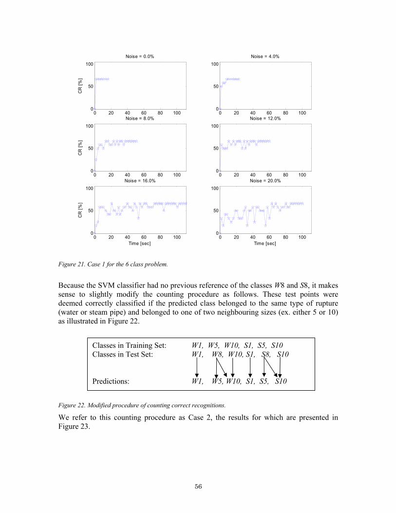
0 20 40 60 80 1000

50

100Noise = 0.0%

CR

[%]

0 20 40 60 80 1000

50

100Noise = 4.0%

0 20 40 60 80 1000

50

100Noise = 8.0%

CR

[%]

0 20 40 60 80 1000

50

100Noise = 12.0%

0 20 40 60 80 1000

50

100Noise = 16.0%

Time [sec]

CR

[%]

0 20 40 60 80 1000

50

100Noise = 20.0%

Time [sec]

Figure 21. Case 1 for the 6 class problem.

Because the SVM classifier had no previous reference of the classes W8 and S8, it makes sense to slightly modify the counting procedure as follows. These test points were deemed correctly classified if the predicted class belonged to the same type of rupture (water or steam pipe) and belonged to one of two neighbouring sizes (ex. either 5 or 10) as illustrated in Figure 22.

Classes in Training Set: W1, W5, W10, S1, S5, S10 Classes in Test Set: W1, W8, W10, S1, S8, S10 Predictions: W1, W5, W10, S1, S5, S10

Figure 22. Modified procedure of counting correct recognitions.

We refer to this counting procedure as Case 2, the results for which are presented in Figure 23.

56

0 20 40 60 80 1000

50

100Noise = 0.0%

CR

[%]

0 20 40 60 80 1000

50

100Noise = 4.0%

0 20 40 60 80 1000

50

100Noise = 8.0%

CR

[%]

0 20 40 60 80 1000

50

100Noise = 12.0%

0 20 40 60 80 1000

50

100Noise = 16.0%

Time [sec]

CR

[%]

0 20 40 60 80 1000

50

100Noise = 20.0%

Time [sec]

Figure 23. Case 2 for the 6 class problem.

4.2.8 Conclusion SVM classifiers have demonstrated promising results with our formulation of the problem of identifying accident sequences at NPPs. This in turn indicates that SVMs show promise as classifiers for the learning problem of identifying transients. For instance, in the 2 class problem at a noise level of ν = 0%, 100% classification rate (CR) was achieved after just a few seconds of simulated real-time operation at the NPP. For the highest level of noise, ν=20%, the classification accuracy would oscillate between 90-100% after about 60s. The results for the more demanding 6 class problem (when ν=0%) were similar giving a CR of 90-100% after just a few seconds and then stabilized to 100% after about 20s. In the case of ν=20%, the classification rate stabilized to 100% when more than about 85s of the beginning of the sequence was included. The SVM methodology was easy to implement and apply to our problem. Especially if compared to alternative methods such as artificial neural networks (ANNs). Furthermore, SVMs were fast in the training of data and provided good results for our training sets, even though they had few input points.

57

It is important to stress that at this point several adjustments to the implementation of SVMs, which might improve overall performance, have been left unexplored. For instance, only one type of kernel function has been used in the task of training our classifiers. Other kernel functions exist and may be better suited for this specific classification problem. Furthermore, several other (possibly better) methods could be explored in the process of finding optimal parameters. As it was shown in this study, noise has a considerably detrimental effect on efficiency of the classification results. So it could be useful to study the effect of noise reduction techniques applied on experimental signals experiencing high levels of noise.

5 Summary and Future Improvements On the static pattern classification problem set up in the experiments of section 4 the SVM classifiers performed well. However, the methods used in these experiments to not take into account the temporal variations of transients that one would expect to find in real sensor signals. To determine whether this method is sufficiently accurate for on-line monitoring of real processes it would be necessary to extend our experiment to a setup that takes this into account . The most practical of these would be the on-line monitoring of a reactor simulator. In this scenario it would be reasonable to assume some drop in performance of the SVM classifiers. The following is a list of techniques that could increase the performance of the existing implementation of the SVM classifiers.

• Ensemble SVMs – a technique often used in real-life solutions using neural networks. The Aladdin software [15] is a prime example of ensemble neural networks for nuclear power plant diagnostics by transient classification. Recently, similar techniques have been developed in other fields for pattern recognition using SVM classifiers ([52], [53] and [54]). Ensemble SVMs might improve the accuracy of the classifiers.

• In the experiments of this thesis no more than six classes were defined to which

input points could belong to. The current implementation of the SVM classifiers can deal with many-class learning problem of this size (in terms of number of classes). However, this implementation would not scale well for large real-life applications consisting of many more classes. Instead, one would have to better techniques that decompose these learning problems to sub-problems with fewer classes. A comparative study of such techniques using neural networks can be found in [55]. In the Aladdin project a new technique was devised called ARTD: Autonomous Recursive Task Decomposition [16]. Both training times and classification accuracy could be significantly improved for learning problems of many classes.

• In the current implementation, the classifier will always associate input points to

one of the known classes (present in the set of training points). This could be a severe liability in safety-critical application such as fault diagnosis at nuclear

58

power plants. Possibilistic fuzzy clustering would give us a mechanism of reducing the chances of misclassifying an “unknown” event sequence. The classifier could now let us know that it has encountered an unknown event sequence, instead of labeling it as a known event. The Aladdin project uses this technique to deal with the problem of “unknown” event sequences. See [56] for an introduction to fuzzy clustering.

• Techniques that reduce the dimension of the input space (feature selection) could

be useful if presented with high-dimensional input data. Principal Component Analysis (PCA) and Independent Component Analysis (ICA) are examples of such techniques. SVM classifiers are however good at dealing with high-dimensional input data (if compared to for instance neural networks) and might therefore not benefit as much from these types of techniques.

• Using different kernel functions such as sigmoid or polynomial kernels to try to

improve the performance of the currently used radial basis function kernel.

59

6 References [1] M. BEDNARSKI, “Application of inverse models in the diagnostics of nuclear

reactors”. Department of Fundamentals of Machine Design, Silesian University of Technology, Poland.

[2] U.S. Nuclear Regulatory Commission. http://www.nrc.gov . “The Code of Federal Regulations, Part 50, Chapter 15” (10 CFR Part 50).

[3] R. E. UHRIG, “Use of Neural Networks in Nuclear Power Plant Diagnostics”, presented at International Conference of Availability Improvements in Nuclear Power Plants, Madrid, Spain, April 10-16, 1989.

[4] E. B. BARTLETT and R. E. UHRIG, “Nuclear power plant status diagnostics using artificial neural networks”, presented at AI’91, Frontiers of Innovative Computing for the Nuclear Industry, Jackson Lake, Wyoming, September 15-18, 1991.

[5] E. B. BARLETT and R. E. UHRIG, “Nuclear power plant status diagnostics using an artificial neural network”, Nuclear Technology, Vol. 97: pp. 272-281, 1992.

[6] Y. BARTAL, J. LIN and R. UHRIG. “Nuclear power plant transient diagnostics using artificial networks that allow “don’t-know” classification”. Nuclear Technology, 100: pp. 436-449, 1995.

[7] A. BASU. “Nuclear power plant transient diagnostics using a neural network with dynamic node architecture”. MS thesis, Iowa State University. 1992.

[8] S. W. CHEON and S. H. CHANG. “Application of neural networks to a connectionist expert system for transient identification in nuclear power plants”. Nuclear Technology, Vol. 102, 1993.

[9] A. IKONOMOPOULOS, R. E. UHRIG and L. TSOUKALAS. “A hybrid neural network-fuzzy logic approach to nuclear power plant transient identification”, AI’91 Frontiers in Innovative Computing for the Nuclear Industry: pp. 217-226. Jackson, WY; Sept. 15-18, 1991.

[10] J. W. HINES, D. W. MILLER and B. K. HAJEK. “A hybrid approach for detecting and isolating faults in nuclear power plant interacting systems”. Nuclear Technology, 115: pp. 342-358.

[11] A. G. PARLOS, A. F. ATIYA, K. T. CHONG and W. K. TSAI. “Nonlinear identification of process dynamics using neural networks”, Nuclear Technology, 97: pp. 79-96, 1992.

[12] C.H. ROH, H. S. CHANG and H. G. KIM. “Identification of reactor vessel failures using spatiotemporal neural networks”. IEEE Tran. Of Nuclear Science, 43(6): pp. 3223-3229.

[13] E. JEONG, K. FURUTA and S. KONDO. “Identification of transient in nuclear power plant using neural network with implicit time measure”. Proc. Topical Meeting on Computer-Based Human Support Systems, PA, June 25-29, 1995. pp. 467-474.

[14] The Aladdin Project. http://www.ife.no/english/prosjekter/project_details.jsp?projectId=4027&beskrId=1351&nav=2 .

[15] D. ROVERSO, “Plant Diagnostics by Transient Classification: The Aladdin Approach”, International Journal of Intelligent Systems (IJIS), Special Issue on Intelligent Systems for Plant Surveillance and Diagnostics, 2002.

60

[16] D. ROVERSO. “ARTD: Autonomous Recursive Task Decomposition for many-class learning”, International Journal of Knowledge-Based Intelligent Engineering Systems, Volume 6, Number 4, 2002.

[17] D. ROVERSO. “Multivariate temporal classification by windowed wavelet decomposition and recurrent neural networks”. International Topical Meeting on Nuclear Plant Instrumentation, Controls and Human-Machine Interface Technologies (NPIC&HMIT 2000), Washington D.C., Nov. 2000.

[18] T. IIJIMA. “Application study of fuzzy logic method for plant-state identification. OECD Halden Reactor Project, HWR-432, Dec. 1995.

[19] K.-C. KWON, J.-H. KIM and P.-H. SEONG. “Hidden markov model-based real-time transient identification in nuclear power plants”. International Journal of Intelligent Systems, Vol. 17: pp. 791-811, 2002.

[20] J. LIN, Y. BARTAL and R. UHRIG. “Using similarity based formulas and genetic algorithms to predict severity of nuclear power plant transients”. Proc. 9th Power Plant Dynamics, Control & Testing Symposium. Knoxville, TN. pp. 53.01-53.09, May 24-26, 1995.

[21] N. ZAVALJEVSKI and K. C. GROSS. “Support vector machines for nuclear reactor state estimation”. Paper submitted for presentation at the ANS International Topical Meeting on “Advances in Reactor Physics and Mathematics and Computation into the Next Millennium”; Pittsburgh, Pennsylvania, USA. May 7-11, 2000.

[22] F. ROSENBLATT, “The Perceptron, a Perceiving and Recognizing Automaton”, Project PARA, Cornell Aeronautical Lab. Rep., no. 85-640-1, Buffalo, NY, (1957).

[23] MINSKY, M.L. and S.A. PAPERT, Perceptrons, Cambridge, M.A.: MIT Press, 1969.

[24] V.N. VAPNIK, The Nature of Statistical Learning Theory, New York, Springer-Verlag (1995).

[25] A.B.J. NOVIKOFF, “On Convergence Proofs of Perceptrons”, Proceedings of the Symposium on the Mathematical Theory of Automata, Polytechnic Institute of Brooklyn, Vol. 12, pp. 615-622, 1962.

[26] T. HASTIE et .al., The Elements of Statistical Learning – Data Mining, Inference and Prediction, Springer-Verlag, 2001.

[27] V. N. VAPNIK and A. JA. CHERVONENKIS, ”On the uniform convergence of relative frequencies of events to their probabilities”, Theory Probab. Apl., 16, pp. 264-280, 1971.

[28] V. N. VAPNIK and A. JA. CHERVONENKIS, “Necessary and sufficient conditions for the uniform convergence of the means to their expectations”, Theory Probab. Apl., 26, pp. 532-553, 1981.

[29] V. N. VAPNIK and A. JA. CHERVONENKIS, “The necessary and sufficient conditions for consistency of the method of empirical risk minimization” (in Russian), Yearbook of the Academy of Sciences of the USSR on Recognition, Classification, and Forecasting, 2, pp. 217-249, Nauka, Moskow, pp. 207-249, 1989. (English translation: “The necessary and sufficient conditions for consistency of the method of empirical risk minimization”, Pattern Recogn. And Image Analysis, 1, (3), pp. 284-305, 1991.

[30] V.N.VAPNIK and A. CHERVONENKIS, “The necessary and sufficient conditions for consistency of the method of empirical risk minimization”, Yearbook of the

61

Academy of Sciences of the USSR on Recognition, Classification and Forecasting, 2, pp. 217-249, Nauka, Moscow, pp. 207-249, (In Russian), 1989.

[31] V.N. VAPNIK, Statistical Learning Theory, New York, Wiley (1998). [32] M. PONTIL, R. RIFKIN & T. EVGENIOU, “From Regression to Classification in

Support Vector Machines, ESANN ’99 Proceedings, pp. 225-230, April 1999. [33] C. J. C. BURGES, “A Tutorial on Support Vector Machines for Pattern

Recognition”, Knowledge Discovery and Data Mining Discovery 2, pp. 121-167, 1998.

[34] N. CRISTIANINI, J. SHAWE-TAYLOR, An Introduction to Support Vector Machines and other kernel-based learning methods, Cambridge University Press (2000).

[35] B. SCHÖLKOPF, “Statistical Learning and Kernel Methods”, Microsoft Research, Technical Report MSR-TR-2000-23, Feb. 2000.

[36] K.-R. MÜLLER et al., “An Introduction to Kernel-Based Learning Algorithms”, IEEE Transactions On Neural Networks, Vol. 12, No. 2, March 2001.

[37] V.N. VAPNIK and A. JA. CHERVONENKIS, Theory of Pattern Recognition (in Russian), Moscow, Nauka (1974).

[38] C. J. C. BURGES and B. SCHÖLKOPF. “Improving the accuracy and speed of support vector learning machines”. In M. MOZER, M. JORDAN and T. PETSCHE, editors, Advances in Neural Information Processing Systems 9, pp. 375-381, Cambridge, MA, 1997. MIT Press.

[39] C. CORTES and V. VAPNIK. “Support vector networks”, Machine Learning, 20, pp. 273-297, 1995.

[40] J. FRIEDMAN. “Another approach to polychotomous classification. Technical report, Stanford University, UA, 1996.

[41] C.-W. HSU and C.-J. LIN. “A Comparison of Methods for Multi-Class Support Vector Machines”. IEEE Transactions on Neural Networks, 13 (2002), pp. 415-425.

[42] J. CHAO et al., “The MAAP Code: What is it, what has it accomplished, and how can it be used in the future?”, ANS Meeting, Reno, 19-20 June 1996. Registered users can go to http://www.maap4.com/ .

[43] C.-C. CHANG and C.-J. LIN, “LIBSVM – A Library for SVMs”, C Library with additional matlab toolbox, http://www.csie.ntu.edu.tw/~cjlin/libsvm/ .

[44] J. C. PLATT. “Fast Training of Support Vector Machines Using Sequential Minimal Optimization”. In B. Schölkopf, C. J. C. Burges and A. J. Smola, editors, Advances in Kernel Methods – Support Vector Learning, Cambridge, MA, 1998. MIT Press.

[45] C.-C. CHANG et al., “A Practical Guide to Support Vector Classification”, http://www.csie.ntu.edu.tw/~cjlin/libsvm/ .

[46] W.S. SARLE (Maintained by), “The Neural Network FAQ”, ftp://ftp.sas.com/pub/neural/FAQ.html, May 2002.

[47] The MathWorks Inc, Neural Network Toolbox Documentation, http://www.mathworks.com/access/helpdesk/help/toolbox/nnet/.

[48] M.S. PACKIANATHER, P.R. DRAKE and H. ROWLANDS, “Optimizing The Parameters of Multilayered Feedforward Neural Networks Through Taguchi Design Of Experiments”, Quality And Reliability Engineering International 2000; 16: pp.461-473.

[49] R. Roy, A Primer on the Taguchi Method. Van Nostrand Reinhold: New York, 1990.

62

[50] M. VAN VEELEN, J.A.G. NIJHUIS and L. SPAANENBURG, “Neural Network Approaches to Capture Temporal Information”, in Dubois, D.M., Computing Anticipatory Systems, Proceedings of the CASYS ’99, American Institute Of Physics, pp. 361-371, 2000.

[51] U. HAUPTMANNS and W. WERNER, Engineering Risks, Springer-Verlag, Berlin, Heidelberg (1991).

[52] H.-M. JE, D. KIM and S. Y. BANG. “Human Face Detection in Digital Video Using SVM Ensemble”, Neural Processing Letters, 17: pp. 239-252, 2003.

[53] B. HEISELE, T. SERRE, S. PRENTICE and T. POGGIO. “Hierarchical classification and feature reduction for fast face detection with support vector machines”. Pattern Recognition, 36: pp. 2007-2017, 2003.

[54] H.-C. KIM, S. PANG, H.-M. JE, D. KIM and S. Y. BANG. “Constructing support vector machine ensemble”. Recognition, 36: pp. 2757-2767, 2003.

[55] G. AUDA and M. KAMEL. ”Modular Neural Network Classifiers: A Comparative Study”, Journal of Intelligent and Robotic Systems, 21: pp. 117-129, 1998.

[56] F. HÖPPNER, F. KLAWONN, R. KRUSE and T. RUNKLER. Fuzzy Cluster Analysis. Wiley, Chichester, 1999.

63

A. Literature Review of Support Vector Machines This literature review is aimed at people who would like to know more about support vector machines and related fields. It features many of the books, tutorial, online resources, etc. that were used throughout this thesis. A short description is written for each reference in which I try to punctuate resources that are particularly suitable as introductory material. Books N. CRISTIANINI, J. SHAWE-TAYLOR. An Introduction to Support Vector Machines and other kernel-based learning methods, Cambridge University Press (2000).

• A comprehensive overview of how SVMs work with some description of the underlying theory that motivates their use. The authors have a tendency of overusing formal definitions making certain sections of the book hard reading for the novice. They have section on applications of SVMs and how to implement them.

V. KECMAN. Learning and Soft Computing: Support Vector Machines, Neural Networks and Fuzzy Logic Models, Cambridge University Press (2001).

• Introductory book describing several methodologies (of which SVMs are one) in the field of soft computing. Tends to be overly verbose but requires no prior knowledge of soft computing. For this reason it is suitable for the complete novice. The book tries to illustrate how SVMs, ANNs and Fuzzy Logic Systems (FLS) are parts of a connected whole. The theory and algorithms are illustrated by practical examples and case studies.

B. SCHÖLKOPF & A. J. SMOLA. Learning with Kernels – Support Vector Machines, Regularization, Optimization, and Beyond, The MIT Press (2002).

• In-depth and comprehensive account of SVMs and related methodologies. This book serves as a good reference but may be inappropriate for people new to the field. Mathematically heavy and concerned with many advanced topics. It has a good section with exercises after each chapter. The exercises range from easy to still unanswered (open) questions.

V. N. VAPNIK. The Nature of Statistical Learning Theory, New York, Springer-Verlag (1995).

• Excellent introduction to SVMs and the underlying theory that motivate their use. Focuses particularly on statistical learning theory. Unlike most books today it is not written in Word (or similar word processor), probably with Latex, making it a joy to read. The resulting typographical lucidity complements the author’s broad knowledge and pedagogical writing style, making this the definitive introduction to SVMs and Statistical Learning Theory.

V. N. VAPNIK. Statistical Learning Theory, New York, Wiley (1998).

• Includes many of the proofs and definitions that the “The Nature of Statistical Learning Theory” left out; as well as a wealth of new material. Provides a

64

theoretical foundation for SVMs and other learning machines. A must have reference on Statistical Learning Theory and Support Vector Machines!

A. J. SMOLA. P. L. BARTLETT, B. SCHÖLKOPF, and D. SHUURMANS, eds. Advances in Large Margin Classifiers, The MIT Press (2000).

• Attempts to provide a first overview of Large Margin Classifiers (SVMs belong to this category). Includes selected articles from the Neural Information Processing Systems (NIPS) conference (1998) held in Breckenridge, Colorado. Freely available at http://www.kernel-machines.org/nips98/lmc-book.pdf.

Internet Resources http://www.kernel-machines.org/index.html

• Probably the biggest repository of information (and links) on SVMs and related methods.

http://www.svms.org/

• A collection of links to information concerning SVMs and related methods. http://www.support-vector.net/

• Homepage of the book “Introduction to Support Vector Machines and other Kernel-based learning methods”.

http://www.kernel-methods.net/

• Homepage of the new book “Kernel Methods for Pattern Analysis” by J. Shawe-Taylor and N. Cristianini, Cambridge University Press, 2004.

http://www.support-vector.ws/html/downloads.html .

• Complementary website to Kecman’s book with Matlab toolboxes that introduce NNs and SVMs.

Tutorials Links to the following tutorials can be found at http://www.kernel-machines.org. C. J. C. BURGES. “A Tutorial on Support Vector Machines for Pattern Recognition”, Knowledge Discovery and Data Mining Discovery 2, pp. 121-167, (1998).

• A good tutorial on C-SVMs (SVM formulation for pattern recognition problems). Prior knowledge of nonlinear optimization theory and basic linear algebra is recommended.

B. SCHÖLKOPF. “Statistical learning and kernel methods”, MSR-TR 2000-23, Microsoft Research, 2000.

• Support Vector Machines for both classification and regression (and related topics such as kernels) are described in these lecture notes.

65

B. SCHÖLKOPF et al. “An introduction to kernel-based learning algorithms”, IEEE Neural Networks, 12(2), pp. 181-201 or http://mlg.anu.edu.au/~raetsch/ps/review.pdf , (2001).

• An introduction to Support Vector Machines, Kernel Fisher Discriminant analysis, and Kernel Principal Component Analysis (PCA).

A. J. SMOLA and B. SCHÖLKOPF. “A Tutorial on Support Vector Regression”, NeuroCOLT Technical Report NC-TR-98-030 or http://www.kernel-machines.org/papers/tr-30-1998.ps.gz , (1998).

• A Tutorial on Support Vector Regression. P.-H. CHEN, C.-J. LIN and B. SCHÖLKOPF. “A Tutorial on ν-Support Vector Machines”, http://www.csie.ntu.edu.tw/~cjlin/papers/nusvmtutorial.pdf , (2003).

• A Tutorial on ν-Support Vector Machine. Software SVMLib – A Library for SVMs by C.-C. CHANG and C.-J. LIN.

• Stable and well-maintained C++ and Java library supporting C-SVC / ν-SVC

(classification), ε-SVR / ν-SVR (regression), one-class SVMs (distribution estimation) and more.

• Implementation based on cutting-edge techniques. • Python, Matlab, Perl and Ruby interfaces.

For more software see http://www.kernel-machines.org/software.html. Publications For a list of online repositories of SVM related publications see section “Internet Resources”. Below is a list of publications found related to SVMs used in the field of nuclear and reactor physics. N. ZAVALJEVSKI and K. C. GROSS, “Sensor Fault Detection in Nuclear Power Plants Using Multivariate State Estimation Technique and Support Vector Machines”, 2000. Available at the KTH library: Studsvik collection. N. ZAVALJEVSKI and K. C. GROSS, “Support Vector Machines for Nuclear Reactor State Estimation”, 2000. Available at the KTH library: Studsvik collection. Journals and Organisations Below is a list of journals that publish material regarding support vector machines - both theoretical and applied. Most of the descriptions of these journals are taken directly from their official site and are put in quotation marks. Journal of Machine Learning Research

• International forum for the publication of articles in all areas of machine learning.

66

• http://jmlr.csail.mit.edu/ Neural Computation

• “Neural Computation disseminates important, multidisciplinary research results and reviews of research areas in neural computation…”

• http://neco.mitpress.org/ IEEE Transactions on Neural Networks

• “…theory, design, application and development of biologically and linguistically motivated computational paradigms involving neural networks, including connectionist systems, genetic algorithms, evolutionary programming, fuzzy systems, and hybrid intelligent systems in which these paradigms are contained.”

• http://www.ieee.org/portal/site/mainsite/menuitem.818c0c39e85ef176fb2275875bac26c8/index.jsp?&pName=corp_level1&path=pubs/transactions&file=tnn.xml&xsl=generic.xsl

NeuroCOLT (Neural Networks and Computational Learning Theory)

• “…the Working Group is to demonstrate the effectiveness of technologies that arise from a deep understanding of the performance and implementation of learning systems on real world data.”

• http://www.neurocolt.com/ Pattern Recognition – The Journal of the Pattern Recognition Society

• “…primary forum for the exchange of information on pattern recognition research among the many varied engineering, mathematical and applied professions which make up this unique field.”

• http://www.elsevier.com/ Pattern Recognition Letters – An Official Publication of the International Association for Pattern Recognition

• “Pattern Recognition Letters aims at rapid publication of concise articles of a broad interest in pattern recognition. Subject areas include all the current fields of interest represented by the Technical Committees of the International Association of Pattern Recognition, and other developing themes involving learning and recognition.”

• http://www.elsevier.com/ Neural Networks – The Official Journal of the International Neural Network Society, European Neural Network Society and Japanese Neural Network Society

• “Neural Networks is an international journal appearing nine times each year that publishes original research and review articles concerned with the modelling of brain and behavioral processes and the application of these models to computer and related technologies.”

• http://www.elsevier.com Neural Processing Letters

67

• “Neural Processing Letters is an international journal publishing research results and innovative ideas in all fields of artificial neural networks.”

• http://www.kluweronline.com/issn/1370-4621/contents Machine Learning

• “Machine Learning is an international forum for research on computational approaches to learning.”

• http://www.kluweronline.com/issn/0885-6125/contents

68