Exact Simulation of Stochastic Volatility and other …finmath.stanford.edu/seminars/documents/Broadie.pdfExact Simulation of Stochastic Volatility and ... method for the exact simulation

Exact Simulation of Stochastic Volatility and

other Affine Jump Diffusion Processes

Mark Broadie

Columbia University, Graduate School of Business, 415 Uris Hall, 3022 Broadway, New York, NY,10027-6902, [email protected]

Ozgur Kaya

Columbia University, Department of Industrial Engineering and Operations Research, 500 West 120thStreet, New York, NY, 10027-6699, [email protected]

First draft: July 23, 2003

This version: September 29, 2004

Abstract

The stochastic differential equations for affine jump diffusion models do not yield exact solutions that

can be directly simulated. Discretization methods can be used for simulating security prices under these

models. However, discretization introduces bias into the simulation results and a large number of time

steps may be needed to reduce the discretization bias to an acceptable level. This paper suggests a

method for the exact simulation of the stock price and variance under Heston’s stochastic volatility

model and other affine jump diffusion processes. The sample stock price and variance from the exact

distribution can then be used to generate an unbiased estimator of the price of a derivative security. We

compare our method with the more conventional Euler discretization method and demonstrate the faster

convergence rate of the error in our method. Specifically, our method achieves an O(s−12 ) convergence

rate, where s is the total computational budget. The convergence rate for the Euler discretization

method is O(s−13 ) or slower, depending on the model coefficients and option payoff function.

Subject Classifications: Simulation, efficiency: exact methods. Finance, asset pricing: computational

methods.

Acknowledgement: This paper was presented at seminars at Columbia University, the sixth Monte

Carlo and Quasi-Monte Carlo Methods in Scientific Computing conference, and INFORMS Annual

Meeting in Atlanta. We thank seminar participants and an anonymous referee for helpful comments

and suggestions. This work was supported in part by NSF grant DMS-0074637.

1 Introduction

Financial models usually specify the dynamics of the state variables, e.g., stock price, volatility and

interest rate, as stochastic differential equations (SDE). If these SDEs yield closed form solutions, then

Monte Carlo simulation can be used to generate an unbiased estimator of the price of a derivative

security. When using Monte Carlo simulation, many sample paths of the state variables are generated

and the payoff of the derivative is evaluated for each path. Discounting and averaging over all paths

gives an estimator of the derivative price. The error in the Monte Carlo estimator can be calculated

using the central limit theorem and converges to zero as the number of sample paths used increases. If

generating each sample path requires roughly equal amount of time, then the convergence rate for such

an unbiased Monte Carlo estimator is O(s−12 ) where s is the total computational budget.

If the SDEs that define the dynamics of the state variables do not yield closed form solutions, it is

still possible to use Monte Carlo simulation by discretizing the time interval and simulating the state

process dynamics on this discrete time grid. However, the approximation of continuous time processes by

discrete time processes introduces bias into the simulation estimator. This bias causes several important

problems when estimating the prices or greeks of derivative securities. First, since the magnitude of

the bias is unknown, it is difficult to obtain valid confidence intervals. Second, many time steps may

be necessary to reduce the bias to an acceptable level, and even more computational effort is needed

to verify that the bias is small enough. Finally, both the number of time steps and number of sample

paths need to be increased together in order to decrease the total error of the simulation estimator, but

the optimal choice of these parameters is difficult to specify in advance. Duffie and Glynn [12] study

optimal rules for allocating the total computational budget between the number of time steps and the

number of simulation trials. They show that, under some regularity conditions, the error for a first

order method such as Euler discretization has O(s−13 ) convergence,

In this paper, we propose a method that recovers the O(s−12 ) convergence rate of an unbiased

Monte Carlo estimator for simulating derivative prices under some affine jump diffusion models. We

first consider the stochastic volatility (SV) model of Heston [19], which models the variance as a square-

root process that is correlated with the stock price. Scott [29] uses Fourier inversion methods to sample

from the integral of a square-root process in an interest rate setting. Willard [31] observes that the

stock price is lognormally distributed conditional on a path of the Brownian motion driving the variance

1

process. A similar ‘mixing result’ was independently discovered in Romano and Touzi [28]. We build

on the ideas from these papers to generate an exact sample from the distribution of the terminal stock

price. We first generate a sample from the final value of the variance. Then using Fourier inversion

methods and conditioning, we get a sample from the integral of the variance. Finally, conditional on

the values for the variance process, we are able to generate a sample from the stock price. We also show

how to extend the method for models involving jumps in addition to the stochastic volatility. Strong

empirical evidence of stochastic volatility and jumps in financial markets is documented in many recent

papers, including Bates [6], Bakshi et al. [4], Chernov et al. [9], Eraker et al. [15], Pan [26] and others.

Some other authors used Monte Carlo simulation for pricing derivatives under the stochastic volatil-

ity models. When the stock price and volatility are instantaneously uncorrelated, Hull and White [20]

show that the stock price has a lognormal distribution conditional on the integral of the variance process.

They write the price of a call option as a Black-Scholes price given the integral of the variance. They

simulate paths of the variance process and find the unconditional price of the option by taking the

average of the conditional Black-Sholes prices. Willard [31] considers the case when the stock price and

volatility are instantaneously correlated. He observes that the stock price is lognormally distributed

conditional on the entire path of the Brownian motion driving the variance process, and the call option

price can be written as a Black-Scholes price conditional on this path. He simulates the variance process

on a discrete time grid and uses conditional Monte Carlo to get the option price. His method still suffers

from discretization bias because of the discretization of the variance process. Heath and Platen [18]

propose a variance reduction technique based on Ito calculus and show how their method can be applied

for simulation under Heston’s stochastic volatility model. Their method uses discretization methods to

simulate the state processes, and therefore does not eliminate the discretization bias.

The rest of the paper is organized as follows: Section 2 introduces the SV model dynamics and Euler

discretization method. Section 3 is a step by step introduction to our method for exact simulation. In

Section 4, we give some numerical results and compare our method to Euler discretization. In Section 5,

we show that the efficiency of our simulation method can be further improved using conditional Monte

Carlo techniques. Section 6 shows how to extend the method to models that involve jumps. In Section

7, we give an application of the exact simulation algorithm to the pricing of forward start options. The

derivation of the characteristic function of the integral of the variance is given in the Appendix.

2

2 SV Model and Euler Discretization

2.1 Specification of the SV Model

Heston’s model [19] is based on the following equations, which represent the dynamics of the stock price

and the variance processes under the risk-neutral measure:

dSt = rStdt +√

VtSt

[ρdW

(1)t +

√1− ρ2dW

(2)t

](1)

dVt = κ(θ − Vt)dt + σv

√VtdW

(1)t . (2)

The first equation gives the dynamics of the stock price: St denotes the stock price at time t, r is

the risk neutral drift,√

Vt is the volatility. The second equation gives the evolution of the variance

which follows the square-root process: θ is the long-run mean variance, κ represents the speed of mean

reversion, and σv is a parameter which determines the volatility of the variance process. W(1)t and

W(2)t are two independent Brownian motion processes, and ρ represents the instantaneous correlation

between the return process and the volatility process.

2.2 Euler Discretization

Euler discretization can be used to approximate the paths of the stock price and variance processes on

a discrete time grid. Let [0 = t0 < t1 < . . . < tM = T ] be a partition of time interval into M equal

segments of length ∆t, i.e, ti = iT/M for each i = 0, 1, . . . , M . The discretization for the stock price

process is:

Sti = Sti−1 + rSti−1∆t +√

Vti−1Sti−1

[ρ∆W

(1)ti

+√

1− ρ2∆W(2)ti

](3)

where ∆W(j)ti

= W(j)ti−W

(j)ti−1

, j = 1, 2. The discretization for variance process is:

Vti = Vti−1 + κ(θ − Vti−1)∆t +√

Vti−1σv∆W(1)ti

. (4)

To simulate the Brownian increments, the fact that each increment W(j)ti

− W(j)ti−1

is independent

of others is used. Each such increment is normally distributed with mean 0 and standard deviation√

∆t. In particular, we can simulate these increments by first generating a uniform random variate

3

U and then replacing ∆W(j)ti

by√

∆tF−1(U), where F (x) is the cumulative distribution function of

a standard normal random variable. There are efficient algorithms for accurately approximating the

inverse function of a normal distribution function. We use the algorithm by Moro [25]. For each

increment, we use an independent uniform random variate, so we need a total of 2M uniform random

variates to simulate a path of stock price and variance processes. When using Euler discretization with

a large number of simulation trials and a large number of time steps, the number of uniform random

variates needed may be huge. We use the random number generator by Matsumoto and Nishimura [24],

which has a very long period. To avoid the negative values for variance and stock price, we set these to

zero if we encounter negative values during the simulation.

By repeating this procedure, many paths can be generated. Because no-arbitrage derivative prices

are given by their expected discounted payoffs under the risk-neutral measure, the price of a derivative,

written as E[f(ST )], can be estimated by Monte Carlo simulation using:

1N

N∑

k=1

f(SMT ) (5)

where N is the number of sample paths used in simulation and SMT denotes the simulated value of ST

over each sample path using M time steps. This Monte Carlo estimator converges to the correct price

E[f(ST )] as the number of time steps M and the number of samples N become large.

There are two types of error associated with the Monte Carlo estimator given in (5). First there

is a statistical error which decreases at the rate O(1/√

N). This is due to the central limit theorem:

the standard error of the simulation estimator is σf/√

N where σf is the standard deviation of f(SMT ).

Second, there is a discretization error or discretization bias defined as: |E[f(ST )] − E[f(SMT )]|. This

error is caused by simulation of continuous-time processes using discrete-time approximations. Kloeden

and Platen [22] show that, under the conditions stated in their Theorem 14.5.2, this error decreases at

the rate O(1/M) for Euler discretization. Talay and Tubaro [30], and Bally and Talay [5] give similar

results, and show that the error can be expanded in powers of 1/M under some regularity conditions

on the coefficients of the SDEs and the function f . The conditions for first order convergence do not

hold for the SDEs in (1) and (2), so the actual convergence may be slower in this case.

Duffie and Glynn [12] study the optimal allocation of a computational budget between the number

4

of time steps and number of simulation trials. Their result implies that it is optimal to choose the

number of time steps proportional to the square-root of the number of simulation trials for first order

methods, although the optimal constant of proportionality is left undetermined. They show that with

their allocation rule, the convergence rate of the error for the Euler discretization is O(s−13 ) where s is

the total computational budget. More generally, if p is the convergence order of the bias, then an optimal

allocation has error convergence of O(s−p

2p+1 ). However, since the conditions for first order convergence

do not hold, O(s−13 ) convergence rate is not guaranteed in this case. Indeed, the numerical examples

we consider in Section 4 demonstrate that Euler discretization may achieve a lower convergence rate

depending on the convergence rate of the bias.

There are higher order discretization schemes that can be used instead of Euler for discretization

of stock price and variance processes. For example, the Milstein scheme is a discretization scheme that

achieves second order convergence for the bias under the conditions given in Kloeden and Platen [22].

In theory, such a second order method would improve the convergence of the total simulation error

to O(s−25 ). But again, since the conditions for convergence are not satisfied by the dynamics of the

state variables, this method is not guaranteed to achieve a second order convergence rate. Also, the

convergence is not very smooth. For an example of this for the SV model, see Glasserman [17]. Another

disadvantage of the Milstein scheme is that it is harder to implement and takes more time per replication

than the Euler discretization.

3 Exact Simulation of the SV Model

In this section we give the details of the exact simulation method. In particular, we show how to

generate an exact sample from the distribution of St by conditioning on the values generated by the

variance process.

The stock price at time t, given the values of Su and Vu for u < t, can be written as:

St = Su exp[r(t− u)− 1

2

∫ t

uVsds + ρ

∫ t

u

√VsdW (1)

s +√

1− ρ2

∫ t

u

√VsdW (2)

s

](6)

5

and the variance at time t is given by the equation:

Vt = Vu + κθ(t− u)− κ

∫ t

uVsds + σv

∫ t

u

√VsdW (1)

s . (7)

We go through the following steps to sample from the distribution of (St, Vt):

Exact Simulation Algorithm for the SV Model:

1. Generate a sample from the distribution of Vt given Vu.

2. Generate a sample from the distribution of∫ tu Vsds given Vt and Vu.

3. Recover∫ tu

√VsdW

(1)s from (7) given Vt, Vu and

∫ tu Vsds.

4. Generate a sample from the distribution of St given∫ tu

√VsdW

(1)s and

∫ tu Vsds.

Next we specify the details of each of these steps.

3.1 Sampling from Vt given Vu

The distribution of Vt given Vu for some u < t is up to a scale factor, a noncentral chi-squared distribution

as noted by Cox et al. [11]. The transition law of Vt can be expressed as:

Vt =σ2

v(1− e−κ(t−u))4κ

χ′2d

(4κe−κ(t−u)

σ2v(1− e−κ(t−u))

Vu

), t > u (8)

where χ′2d (λ) denotes the noncentral chi-squared random variable with d degrees of freedom, and non-

centrality parameter λ, and

d =4θκ

σ2v

. (9)

This says that, given Vu, Vt is distributed as σ2v(1 − eκ(t−u))/(4κ) times a noncentral chi-squared

random variable with d degrees of freedom and noncentrality parameter

λ =4κe−κ(t−u)

σ2v(1− e−κ(t−u))

Vu. (10)

Thus, we can sample from the distribution of Vt exactly, provided that we can sample from the noncentral

chi-squared distribution.

Let χ2d denote a chi-squared random variable with d degrees of freedom. Johnson et al. [21] show

6

that for d > 1, the following representation is valid:

χ′2d (λ) = χ

′21 (λ) + χ2

d−1. (11)

To generate χ′2d (λ), d > 1, we can generate χ2

d−1 and an independent standard normal random

variable Z and set

χ′2d (λ) = (Z +

√λ)2 + χ2

d−1. (12)

Thus, sampling from a noncentral chi-squared distribution is reduced to sampling from an ordinary

chi-squared and an independent normal when d > 1.

For any d > 0, a noncentral chi-squared random variable can be represented as an ordinary chi-

squared random variable with a random degrees of freedom parameter. In particular, if N is a Poisson

random variable with mean 12λ, then χ2

d+2N has the same distribution as χ′2d (λ). So, to sample from

χ′2d (λ), we can first generate a Poisson random variable N and then, conditional on N , we can sample

a chi-squared random variable with d + 2N degrees of freedom.

In the simulation of Vt, we use the representation given in (12) when d > 1, and we use the Poisson

method described above otherwise. To sample from the chi-squared distribution, the methods to sample

from gamma distribution can be used since chi-squared is a special case of this distribution. We use

algortihms GS* and GKM3 in Fishman [16] to sample from the gamma distribution. The first of these

is used when the degrees of freedom parameter for chi-squared distribution is less than one, and the

second one is used otherwise.

3.2 Sampling from∫ t

uVsds given Vt and Vu

Once we have a sample for Vt, we want to sample from the distribution of∫ tu Vsds given Vt and Vu.

Scott [29] uses Fourier inversion techniques to invert the characteristic function of this distribution to

sample from the same distribution in an interest rate setting. We follow a similar approach to generate

a sample for the integral. The Laplace transform

E

[exp

(−a∗

∫ t

uVsds

)∣∣∣∣Vu, Vt

]

7

can be derived using the results in Pitman and Yor [27]. Details of the derivation are given in the

appendix. The characteristic function follows by setting a∗ = −ia:

Φ(a) = E

[exp

(ia

∫ t

uVsds

)∣∣∣∣Vu, Vt

]

=γ(a)e

−12

(γ(a)−κ)(t−u)(1− e−κ(t−u))κ(1− e−γ(a)(t−u))

× exp

{Vu + Vt

σ2

[κ(1 + e−κ(t−u))

1− e−κ(t−u)− γ(a)(1 + e−γ(a)(t−u))

1− e−γ(a)(t−u)

]}

×I0.5d−1

[√VuVt

4γ(a)e−0.5γ(a)(t−u)

σ2(1−e−γ(a)(t−u))

]

I0.5d−1

[√VuVt

4κe−0.5κ(t−u)

σ2(1−e−κ(t−u))

] (13)

where γ(a) =√

κ2 − 2σ2ia, d is as given in (9) and Iν(x) is the modified Bessel functon of the first kind.

The probability function can be computed using Fourier inversion methods. If we let V (u, t) denote

the random variable that has the same distribution as the integral∫ tu Vsds conditional on Vu and Vt,

then we can write (see Feller [14]):

F (x) ≡ Pr{V (u, t) ≤ x} =1π

∫ ∞

−∞

sinux

uΦ(u)du =

2π

∫ ∞

0

sinux

uRe[Φ(u)]du. (14)

We use the trapezoidal rule to compute the probability distribution numerically:

Pr{V (u, t) ≤ x} =hx

π+

2π

∞∑

j=1

sinhjx

jRe[Φ(hj)]− ed(h) (15)

where h is a grid size to be set to achieve any desired level of accuracy, and ed(h) is the resulting

discretization error. The trapezoidal rule works well for periodic and other oscillating integrands,

because the errors tend to cancel. The discretization error ed(h) can be bounded above and below by

using Possion summation formula as shown in Abate and Whitt [1]:

0 ≤ ed(h) =∞∑

k=1

[F

[2kπ

h+ x

]− F

[2kπ

h− x

]]≤ F c

[2π

h− x

](16)

8

where F c(x) = 1− F (x).

If we want to achieve a discretization error ε, then the step size should be:

h =2π

x + uε≥ π

uε, where F c(uε) = ε and 0 ≤ x ≤ uε. (17)

Finding the correct uε is not straightforward but the moments of the distribution can easily be found

using the characteristic function in (13). We use the mean plus five or more standard deviations to get

a value with a small tail probability.

To be able to calculate Pr{V (u, t) ≤ x} using (15), we need to determine a point at which the

summation can be terminated. Let N represent the last term to be calculated so that the approximation

becomes

Pr{V (u, t) ≤ x} =hx

π+

2π

N∑

j=1

sinhjx

jRe[Φ(hj)]− ed(h)− eT (N) (18)

where eT (N) denotes the truncation error caused by using N terms in the finite sum. The magnitude

of the characteristic function, |Φ(u)|, has value one at u = 0 and it decreases as u increases. Since

| sin(ux)| ≤ 1, The integrand in (14) is bounded by:

2|Re[Φ(u)]|πu

≤ 2|[Φ(u)]|πu

= β(u). (19)

Since the integrand is oscillating, the bound for the last term gives a good estimate for the truncation

error, i.e. we set eT (N) = hβ(Nh). The summation is terminated at j = N when

|Φ(hN)|N

<πε

2(20)

where ε is the desired truncation error.

It should be noted that very often the error bounds stated above for determination of the grid size

h and the truncation point N are conservative. By trial and error one can get h and N that achieves

the desired accuracy with fewer number of terms.

The hardest and numerically most time consuming part of (15) is the evaluation of the characteristic

function. The characteristic function given in (13) involves two modified Bessel functions of the first

kind, and the one in the numerator has a complex argument. The modified bessel function of the first

9

kind is characterized by the following power series:

Iν(z) =(

12z

)ν ∞∑

j=0

(14z2)j

j!Γ(ν + j + 1)(21)

where Γ(x) is the gamma function and z is a complex number. We used a routine written by Amos [3]

to calculate these functions. The routine uses the power series for small |z|, the asymptotic expansion

for large |z|, the Miller Algorithm normalized by the Wronskian and a Neumann Series for intermediate

magnitudes, and the uniform asymptotic expansion for large orders. The routine can also calculate a

scaled version of the Bessel function, e−|Re(z)|Iν(z) which makes it possible to compute the function

value for very large orders.

The representation of Iν(z) given in (21) is not complete because the function zν , which is a factor

on the right hand side, is a multivalued function and needs precise specification. It is defined to be

exp(ν log z), where the argument of z is given its principal value so that

−π < arg(z) ≤ π.

This is the definition most software packages and the programming library routines uses to calculate

the function value. However, the function Iν(z) defined in this way is discontinuous at each point along

the negative x-axis as are all functions defined on a specific branch of arg(z). So to get around this

problem and accomplish the continuity of the characteristic function, we need to keep track of arg(z)

and change the branch when necessary. We use the following continuation formula from Abramowitz

and Stegun [2] for this purpose which makes it possible to calculate the value of Iν(z) for arg(z) different

than its principal value:

Iν(zemπi) = emνπiIν(z) {m integer}. (22)

As this formula shows, to calculate the function on a different branch, we need to multiply the value on

the principal branch by a factor emπνi.

To simulate the value of the integral, we use the inverse transform method. We generate a uniform

random variable U and then find the value of x for which the Pr{V (u, t) ≤ x} is equal to U . We use a

second order Newton’s method to find the solution for x. This method is used to solve the equations of

10

the form f(x) = 0 using the iteration:

xn+1 = xn − f′(xn)

f ′′(xn)

(1−

√2f(xn)f ′′(xn)

f ′(xn)2

).

The conditional distribution of the integral is approximately normal and the initial guess for x is

calculated using the inverse normal distribution function with the mean and standard deviation of the

correct distribution. The moments of the correct distribution are found using (13). We set the starting

value to a small value such as 0.01 times the mean if the normal value is negative. The first and

second derivatives of the distribution function are calculated numerically using the derivatives of the

approximation (15). The iterative procedure achieves five decimal place accuracy in 3 to 4 iterations.

We use a bisection search method when the above mentioned method fails to converge to true value,

which typically occurs when U is very close to 0 or 1.

3.3 Generating a Sample for St

After having generated samples from Vt and∫ tu Vsds we use (7) to get:

∫ t

u

√VsdW (1)

s =(

1σv

)(Vt − Vu − κθ(t− u) + κ

∫ t

uVsds

). (23)

Furthermore, since the process for Vt is independent of the Brownian motion W(2)t , the distribution

of∫ tu

√VsdW

(2)s given the path generated by Vt is normal with mean 0 and variance

∫ tu Vsds.

Using these two results, we get that the conditional distribution of log St is normal with mean

m(u, t) = log Su +[r(t− u)− 1

2

∫ t

uVsds + ρ

∫ t

u

√VsdW (1)

s

]

and variance

σ2(u, t) = (1− ρ2)∫ t

uVsds.

To generate a sample from St, we generate a standard normal random variable Z and then set:

St = em(u,t)+σ(u,t)Z .

11

We can use the value of St generated in this way to find the price of any derivative that depends on

the value of St. Repeating over many sample paths, taking the average and discounting gives us an

unbiased estimator of the derivative price.

4 Numerical Results

In this section we present some numerical comparisons of the Euler and the exact simulation method

described above. We use a European call option for this purpose. Heston [19] gives a closed form

solution for the price of this option, so we are able to calculate and compare the two methods through

their root-mean-squared (RMS) errors. If α is the simulation estimator used for the derivative price

and α is the true price, then the bias of the estimator is given by (E[α]− α) and the variance is given

by E[(α−E[α])2]. RMS error is then defined as (bias2 + variance)1/2. The bias for Euler discretization

with a specific number of time steps can be estimated using a very large number of simulation trials

to estimate E[α], and then taking the difference with the true price. The variance for each simulation

experiment is estimated by the sample variance of the simulation output.

The simulation experiments in this and the other sections of the paper were performed on a desktop

PC with an AMD Athlon 1.66 GhZ processor and 624 MB of RAM, running Windows XP Professional.

The codes were written in C programming language, and the compiler used was Microsoft Visual

C++ 6.0.

Table 1 gives simulation results for a European call option. The set of parameters for the SV

model are taken from Duffie et al. [13]. These were found by minimizing the mean squared errors for

market option prices for S&P 500 on November 2, 1993. The bias column is estimated using 40 million

simulation runs. The number of time steps for the Euler discretization is set equal to the square-root

of the number of simulation trials.

The time needed for the exact method is more than the Euler discretization for small number of

simulation runs. However, the exact method requires less computation time as the desired accuracy is

increased.

There are some cases for which the bias of the Euler discretization is very large even if a large

number of time steps is used. This is especially true when (2κθ/σ2v) ≤ 1 and σv is large relative to θ. In

this case the variance process for Euler discretization often hits to 0 causing a large discretization bias.

12

Table 1: Simulation Results under the SV Model for a European Call Optiona. Simulation with the Exact Method

No of Simulation Trials RMS Error Computing Time (sec.)10000 0.0750 3.840000 0.0373 15.2

160000 0.0186 60.0640000 0.0093 239.4

2560000 0.0046 955.710240000 0.0023 3822.6

b. Simulation with the Euler Discretization

No of Simulation No of Time Standard RMS ComputingTrials Steps Bias Error Error Time (sec.)

10000 100 0.1543 0.0772 0.1725 0.240000 200 0.1003 0.0381 0.1073 1.9

160000 400 0.0662 0.0189 0.0689 15.2640000 800 0.0395 0.0094 0.0406 121.3

2560000 1600 0.0267 0.0047 0.0272 970.010240000 3200 0.0161 0.0023 0.0163 7758.6

Option parameters: S = 100, K = 100, V0 = 0.010201, κ = 6.21, θ = 0.019, σv = 0.61, ρ = −0.70, r = 3.19%, T = 1.0

year, true option price=6.8061.

Table 2 demonstrates this case. The bias column is estimated using 40 million simulation runs.

As seen from the simulation results in Table 2, significant bias remains in the Euler discretization

even when 3200 time steps are used with 10,240,000 simulation runs. The RMS error for our exact

method with the same number of trials is about 30 times smaller with much less computation time.

Figures 1 and 2 show the convergence of the RMS graphically for both methods. The faster convergence

rate of the exact method is demonstrated by the higher slope in the graphs.

One apparent problem when using Euler discretization is the choice of the number of time steps to

be used in the simulation. Our choice of setting number of the time steps equal to the square-root of the

number of simulation trials is somewhat arbitrary. Duffie and Glynn [12] show that, asymptotically, it is

optimal to increase the number of time steps proportional to the square-root of the number of simulation

trials for first-order methods such as Euler discretization. But the optimal constant of proportionality is

not easy to determine. Ideally, for a specific number of simulation trials, one should choose the number

of time steps such that the magnitude of the discretization bias and the standard error will be close.

Then, as more accuracy is needed, the number of time steps should be increased proportional to the

square-root of the number of simulation trials. This way, simulation estimate converges to the true

13

10−1

100

101

102

103

104

10−3

10−2

10−1

100

Convergence of the RMS Error

Total Simulation Time (seconds)

RM

S E

rror

EulerExact

Figure 1: Convergence of the RMS Errors of the Two Methods for the Option in Table 1 (SV Model)

10−1

100

101

102

103

104

10−2

10−1

100

101



RM

S E

rror

EulerExact


14

Table 2: Simulation Results under the SV Model for a European Call Optiona. Simulation with the Exact Method


160000 0.1464 61.3640000 0.0726 244.5

2560000 0.0362 978.610240000 0.0181 3916.5

b. Simulation with the Euler discretization


10000 100 2.1962 0.6568 2.2923 0.240000 200 1.6413 0.3247 1.6731 1.9

160000 400 1.2151 0.1544 1.2248 15.4640000 800 0.9265 0.0761 0.9296 122.6

2560000 1600 0.7093 0.0379 0.7103 980.410240000 3200 0.5367 0.0188 0.5370 7838.4

Option parameters: S = 100, K = 100, V0 = 0.09, κ = 2.00, θ = 0.09, σv = 1.00, ρ = −0.30, r = 5.00%, T = 5.0 years, true

option price=34.9998.

value with neither of the errors dominating the other. Of course, in practice, we do not usually know

the true value of the quantity we want to estimate and therefore it is not possible to know what the bias

is. Even for the cases where we do know the true value, we might need to do a convergence study with

many simulation trials to estimate the bias. Thus, the choice of the number of time steps is another

shortcoming of the Euler discretization method.

Table 3 shows the bias values for various time steps for the two options considered before. The bias

values are estimated using 40 million simulation runs. For both options, the bias dominates the standard

error when number of time steps, M , is set to the square-root of the number of simulation trials, N .

For the first option, the number of time steps that makes bias and standard error approximately equal

is between√

N and 10√

N , while for the second option this value is greater than 10√

N .

Careful examination of the bias values in Table 3 reveals another problem with the convergence of

the Euler discretization. The bias values do not decrease to half of their values when the number of time

steps are doubled. We mentioned in section 2.2 that the conditions for first order convergence do not

hold for the SDEs in (1) and (2). These examples demonstrate that the convergence for discretization

bias may indeed be significantly slower. As shown in Duffie and Glynn [12], if p is the convergence order

15

Table 3: Effect of the Number of Time Steps in Euler discretizationa. Bias Values for the Option in Table 1No of Simulation Standard Bias Values for Various Time Steps (M)

Trials (N) Error M = 0.1√

N Bias M =√

N Bias M = 10√

N Bias10000 0.0772 10 0.5348 100 0.1543 1000 0.036440000 0.0381 20 0.3897 200 0.1003 2000 0.0225

160000 0.0189 40 0.2667 400 0.0662 4000 0.0163640000 0.0094 80 0.1745 800 0.0395 8000 0.0099

2560000 0.0047 160 0.1156 1600 0.0267 16000 0.006710240000 0.0023 320 0.0739 3200 0.0161 32000 0.0029

a. Bias Values for the Option in Table 2

No of Simulation Standard Bias Values for Various Time Steps (M)

Trials (N) Error M = 0.1√

N Bias M =√

N Bias M = 10√

N Bias10000 0.6568 10 6.0489 100 2.1962 1000 0.840840000 0.3247 20 4.5423 200 1.6413 2000 0.6257

160000 0.1544 40 3.2997 400 1.2151 4000 0.5142640000 0.0761 80 2.4358 800 0.9265 8000 0.3731

2560000 0.0379 160 1.7914 1600 0.7093 16000 0.293510240000 0.0188 320 1.3501 3200 0.5367 32000 0.2273

of the bias, then an optimal allocation has error convergence of O(s−p

2p+1 ). The convergence rate of

the bias for these examples is close to O(1/√

M). Assuming this rate is the real convergence rate, the

convergence rate of the total error for an optimal allocation would be O(s−14 ). In practical cases, a non-

optimal allocation may be used since the real convergence rate of the bias is unknown, leading to even

slower convergence rates. These arguments provide another motivation for using an exact simulation

method instead of biased methods.

5 Conditional Monte Carlo for the SV Model

Willard [31] proposed a conditional Monte Carlo method to improve the efficiency of the simulation

estimators under stochastic volatility models. His method is applicable for path-independent derivatives

that have closed form solutions under the Black-Sholes model. In this section we apply the conditional

Monte Carlo method to improve the efficiency of the exact simulation method we described in Section 3.

We also compare the improved results with the results of Euler discretization in the same setting.

We follow the approach of Willard and use a European call option to demonstrate the conditional

Monte Carlo method. We assume the dynamics of the stock price and the variance processes are as

16

given in (1) and (2). Let BS(S0, σ) denote the Black-Sholes formula for a European call option with

maturity T , strike K and written on a stock with initial price S0 and constant volatility σ. Let σ be

the average volatility of the stock over the time horizon:

σ ≡√

1T

∫ T

0Vsds. (24)

Willard observes that conditional on a path of the Brownian motion driving the variance process,

the price of the call option can be written as

BS(S0ξ, σ√

1− ρ2) (25)

where

ξ = exp(−ρ2

2

∫ T

0Vsds + ρ

∫ T

0

√VsdW (1)

s

). (26)

Then, using the law of iterated expectations, the unconditional price of the option can be written

as:

E[BS

(S0ξ, σ

√1− ρ2

∣∣∣W (1)s

)]. (27)

The notation used emphasizes that the Black-Scholes price inside the expectation is conditional on a

path of the Brownian motion W(1)s . Actually, it is not necessary to condition on the entire path of the

Brownian motion. We can just write:

E

[BS

(S0ξ, σ

√1− ρ2

∣∣∣∣∫ T

0Vsds,

∫ T

0

√VsdW (1)

s

)](28)

since we only need∫ T0 Vsds and

∫ T0

√VsdW

(1)s to compute the Black-Scholes price. We can now use the

above representation to estimate the option price using conditional Monte Carlo.

The above approach can also be used to generate unbiased estimators of the Greeks under the SV

model. For example, to calculate the delta of a European call option, we can differentiate the expression

in (28) and get:

E

[∆

(S0ξ, σ

√1− ρ2

∣∣∣∣∫ T

0Vsds,

∫ T

0

√VsdW (1)

s

)ξ

](29)

where ∆(S, v) denotes the Black-Scholes delta. See Broadie and Glasserman [7] for more details about

17

the pathwise method to estimate option greeks in a Monte Carlo simulation. Extensions of the exact

simulation method in this paper to the development of unbiased simulation estimates of Greeks for

various exotic options are given in Broadie and Kaya [8].

In Section 3, we described the steps to sample from the final variance value VT , and the integral of

the variance value∫ T0 VsdW

(1)s , and also showed how to recover

∫ T0

√VsdW

(1)s given these two. When

using the exact simulation method with conditional Monte Carlo, we can complete these steps and then

use (25) to get the conditional option price. By repeating over many paths and taking the average, we

can get an unbiased estimator of the option price.

When using Euler discretization with conditional Monte Carlo, only the variance process needs to

be simulated using the discretization in (4). Simulation of the stock price is not needed, because after

simulating a path of the variance process, one can use (25) to find the conditional option price. Using

conditional Monte Carlo cuts the simulation time for Euler discretization roughly in half since only one

process is simulated instead of two. However, it does not eliminate the discretization bias because the

variance process is still being simulated on a discrete time grid.

Tables 4 and 5 show the simulation results for the two options considered in the previous section,

this time using conditional Monte Carlo with the exact simulation and Euler discretization methods.

Although the conditional Monte Carlo decreases the simulation time and the standard error for the

Euler discretization, the bias is almost unchanged. Figures 3 and 4 show the convergence of the RMS

errors.

Comparing the RMS error for the exact method using conditional Monte Carlo and unconditional

Monte Carlo, we see that conditional Monte Carlo can lead to significant variance reduction. For the

second option considered, more than 50-fold variance reduction is achieved using conditional Monte

Carlo.

In addition to the conditional Monte Carlo method described above, Willard [31] uses quasi-Monte

Carlo (low-discrepancy) methods, and shows that it results in significant efficiency improvements. Quasi-

Monte Carlo helps in improving the convergence of the simulation error, but it does not decrease or

eliminate the discretization bias. Therefore, qualitative results similar to the ones above will hold in

comparing the exact method and the Euler discretization method when quasi-Monte Carlo is used for

both.

18

10−1

100

101

102

103

104

10−3

10−2

10−1

100



RM

S E

rror

EulerExact


10−1

100

101

102

103

104

10−3

10−2

10−1

100

101



RM

S E

rror

EulerExact


19

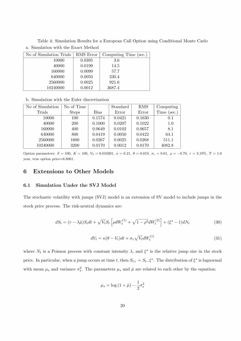
Table 4: Simulation Results for a European Call Option using Conditional Monte Carloa. Simulation with the Exact Method


160000 0.0099 57.7640000 0.0050 230.4

2560000 0.0025 921.610240000 0.0012 3687.4



10000 100 0.1574 0.0421 0.1630 0.140000 200 0.1000 0.0207 0.1022 1.0

160000 400 0.0649 0.0102 0.0657 8.1640000 800 0.0419 0.0050 0.0422 64.1

2560000 1600 0.0267 0.0025 0.0268 511.110240000 3200 0.0170 0.0012 0.0170 4082.8

Option parameters: S = 100, K = 100, V0 = 0.010201, κ = 6.21, θ = 0.019, σv = 0.61, ρ = −0.70, r = 3.19%, T = 1.0

year, true option price=6.8061.

6 Extensions to Other Models

6.1 Simulation Under the SVJ Model

The stochastic volatility with jumps (SVJ) model is an extension of SV model to include jumps in the

stock price process. The risk-neutral dynamics are:

dSt = (r − λµ)Stdt +√

VtSt

[ρdW

(1)t +

√1− ρ2dW

(2)t

]+ (ξs − 1)dNt (30)


√VtdW

(1)t (31)

where Nt is a Poisson process with constant intensity λ, and ξs is the relative jump size in the stock

price. In particular, when a jump occurs at time t, then St+ = St−ξs. The distribution of ξs is lognormal

with mean µs and variance σ2s . The parameters µs and µ are related to each other by the equation:

µs = log (1 + µ)− 12σ2

s

20

Table 5: Simulation Results for a European Call Option using Conditional Monte Carloa. Simulation with the Exact Method


160000 0.0199 60.1640000 0.0100 239.7

2560000 0.0050 958.910240000 0.0025 3835.7



10000 100 2.1046 0.1002 2.1070 0.140000 200 1.5870 0.0469 1.5877 1.0

160000 400 1.2025 0.0227 1.2027 8.4640000 800 0.9154 0.0110 0.9155 64.2

2560000 1600 0.7022 0.0054 0.7022 512.110240000 3200 0.5391 0.0026 0.5391 4086.5

Option parameters: S = 100, K = 100, V0 = 0.09, κ = 2.00, θ = 0.09, σv = 1.00, ρ = −0.30, r = 5.00%, T = 5.0 years, true

option price=34.9998.

and only one of them needs to be specified.

To sample from the final stock price, the jump part and the diffusion part can be simulated separately.

In other words, we can first simulate the diffusion part of the stock price, and then multiply by the

realized jump sizes. This makes it possible to extend the exact simulation method to simulate under

the SVJ model.

To generate a sample for the derivative payoff which has maturity T , we use the following procedure:

21

Exact Simulation Algorithm for the SVJ Model:

1. Disregard the jump part, and simulate the stock price ST as in the SV model using the

exact simulation method described in Section 3.

2. Generate a Poisson random variable with mean (λT ) to determine the number of jumps

occured in the time horizon, call this number J .

3. Generate independent jump sizes ξsi , for i = 1, . . . , J , from the lognormal distribution with

mean µs and variance σ2s .

4. Find the adjusted final stock price ST by multiplying the price from step 1 with the jump

sizes, i.e., set ST = ST∏i=J

i=1 ξsi .

5. Compute the derivative payoff using ST .

Table 6 gives numerical results for a European call option using exact simulation and Euler discretiza-

tion methods. The model parameters are taken from Duffie et al. [13], these are fitted parameters for

S&P 500 on a particular day. The bias of the Euler discretization method is relatively small for the set

of parameters used. Therefore, we choose the number of time steps, M , to be equal to 0.1√

N , where

N is the number of simulation trials. The bias column is estimated using 500 million simulation runs.

Figure 5 shows the convergence of the RMS errors for the two simulation methods used. The exact

method has a better RMS error than the Euler discretization method except only when less than one

second of computation time is used.

6.2 Simulation Under the SVCJ Model

The SVCJ model introduced in Duffie et al. [13] is similar to the SVJ model, but it also includes jumps

in the variance process. The governing equations are:

dSt = (r − λµ)Stdt +√

VtSt

[ρdW

(1)t +

√1− ρ2dW

(2)t

]+ (ξs − 1)dNt (32)


√VtdW

(1)t + ξvdNt (33)

where Nt is again a Poisson process with constant intensity λ, ξs is the relative jump size of the

stock price, and ξv is the jump size of the variance. The jumps in stock price and the variance occur

concurrently, and their magnitudes have a correlation determined by the parameter ρJ . The distribution

22

Table 6: Simulation Results under the SVJ model for a European Call Optiona. Simulation with the Exact Method


160000 0.0560 9.1640000 0.0280 36.2

2560000 0.0140 144.710240000 0.0070 579.4



10000 10 0.5902 0.2480 0.6402 0.140000 20 0.2834 0.1169 0.3065 0.3

160000 40 0.1322 0.0575 0.1442 1.9640000 80 0.0557 0.0283 0.0625 12.6

2560000 160 0.0196 0.0141 0.0241 97.710240000 320 0.0043 0.0070 0.0082 776.1

Option parameters: S = 100, K = 100, V0 = 0.008836, κ = 3.99, θ = 0.014, σv = 0.27, ρ = −0.79, λ = 0.11, µ =

−0.12, σs = 0.15, r = 3.19%, T = 5.0 years, true option price=20.1642.

of ξv is exponential with mean µv. Given ξv, ξs is lognormally distributed with mean (µs + ρJξv) and

variance σ2s . The parameters µs and µ are related to each other by the equation:

µs = log [(1 + µ)(1− ρJµv)]− 12σ2

s

and only one of them needs to be specified.

The jumps in variance prevent us from using the same method as in SVJ model but it is still possible

to extend the method to generate exact simulation estimators under the SVCJ model. We need to divide

the simulation according to the jump occurences and simulate the values of variance and stock price at

each jump time.

To generate a sample for the derivative payoff which has maturity T , we use the procedure described

below. We denote the initial stock price by S0, the initial variance value by V0, and the current time by t0:

23

Exact Simulation Algorithm for the SVCJ Model:

1. Simulate a Poisson process with arrival rate λ and determine the time of the next jump,

denote this time by tj . If tj > T then set tj = T .

2. Disregard the jump part, and simulate the variance value Vtj and stock price Stj using the

exact simulation method described in Section 3 using a time interval of ∆t = tj − t0.

3. If tj = T then set ST = Stj and go to step 6. Otherwise generate ξv by sampling from an

exponential distribution with mean µv. Update the variance value by setting Vtj = Vtj +ξv.

4. Generate ξs by sampling from a lognormal distribution with mean (µs +ρJξv) and variance

σ2s . Update the stock price by setting Stj = Stjξ

s.

5. Set S0 = Stj , V0 = Vtj , t0 = tj and go to step 1.

6. Compute the derivative payoff using ST .

Dividing the simulation horizon and using more time steps affects the computation speed, therefore

the simulation of SVCJ model is slower than SV or SVJ models. If, for example, the arrival rate of

jumps is one per year, then the simulation of a 5 year option will be about 5 times slower. Some of the

advantage of simulating the stock price over a long horizon is lost, but still, the method is practical and

provides unbiased simulation estimators of derivative prices.

The Fourier inversion step in the exact simulation method may run into some problems when the

simulation interval is too small. Such cases may occur in the simulation of SVCJ model when two jumps

are very close to each other or when a jump is too close to maturity. If the simulation interval is less

than 0.01 year, instead of using the exact simulation method, we use Euler discretization with 100 time

steps. This introduces negligible bias into simulation estimate and solves the complexities for small

time intervals.

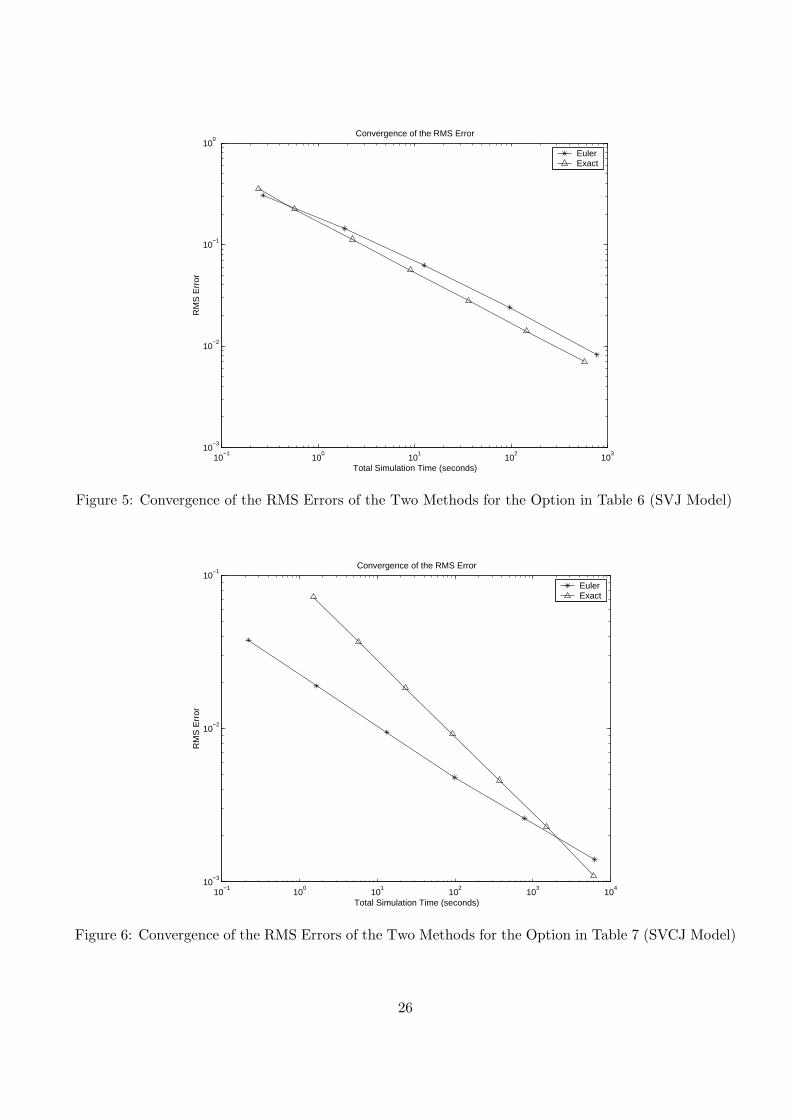
Table 7 gives some numerical results for simulation under the SVCJ model with the exact and Euler

discretization methods. The model parameters are again the fitted parameters for S&P 500 and taken

from Duffie at al. [13]. For the Euler discretization, we choose the number of time steps, M , to be equal

to 0.1√

N , where N is the number of simulation trials. The bias column is estimated using 500 million

simulation runs. Figure 6 shows the convergence of the RMS errors for both methods. In this case, the

point where the exact method starts dominating Euler discretization is closer to the right of the graph.

This is both because the bias in the Euler discretization is relatively small for this set of parameters,

24

and also because the jumps increase the computation time of the exact simulation method.

Table 7: Simulation Results under the SVCJ model for a European Call Optiona. Simulation with the Exact Method


160000 0.0184 23.3640000 0.0092 93.5

2560000 0.0046 373.010240000 0.0023 1491.340960000 0.0011 5967.5



10000 10 0.0148 0.0729 0.0744 0.140000 20 0.0090 0.0367 0.0378 0.2

160000 40 0.0050 0.0183 0.0190 1.6640000 80 0.0024 0.0092 0.0095 13.3

2560000 160 0.0014 0.0046 0.0048 98.810240000 320 0.0012 0.0023 0.0026 784.440960000 640 0.0008 0.0011 0.0014 6254.7

Option parameters: S = 100, K = 100, V0 = 0.007569, κ = 3.46, θ = 0.008, σv = 0.14, ρ = −0.82, λ = 0.47, µ =

−0.1, σs = 0.0001 µv = 0.05, ρJ = −0.38, r = 3.19%, T = 1.0 year, true option price=6.8619.

7 An Application: Pricing of Forward Start Options

The exact simulation method of this paper can be applied to the pricing of many exotic options. To

illustrate this point, in this section we consider the pricing of forward start options. These are options

whose strike is set at a future date. In particular, if T1 is the time when strike is set, T2 is the option

expiration, Si is the stock price at time Ti, and k is the constant that determines the strike, then the

forward start option payoff at time T2 is given by (S2 − kS1)+. For example, if k = 1, then at time

T1, the option becomes an at-the-money option with expiration T2. Kruse and Nogel [23] recently

developed an expression for this option under the SV model by integrating the pricing formula with the

conditional density of the variance value at time T1. However, numerical evaluation of their expression

is quite complicated since it includes another level of integration to already complex integrals in the

Heston formula. Therefore, simulation may be considered as a more practical alternative for finding

25

10−1

100

101

102

103

10−3

10−2

10−1

100



RM

S E

rror

EulerExact

Figure 5: Convergence of the RMS Errors of the Two Methods for the Option in Table 6 (SVJ Model)

10−1

100

101

102

103

104

10−3

10−2

10−1



RM

S E

rror

EulerExact

Figure 6: Convergence of the RMS Errors of the Two Methods for the Option in Table 7 (SVCJ Model)

26

prices and sensitivities of this option. Also, for the SVJ and SVCJ models, no similar expressions are

available and so other numerical methods are necessary for pricing forward start options under these

models.

It is straightforward to price a forward start option using simulation: for each path, simulate the

stock price values at T1 and T2, and then evaluate the payoff function using these two values. How-

ever, we can use an alternative method for simulating a forward start option that will allow us to get

more efficient estimators. Note that at time T1, we know the stock price, strike and the expiration

of the option. Therefore the option price at time T1 can be written using closed form formulas. Let

CE(S,K, T, V ) denote the price of a European call option with initial stock price S, strike K, time to

expiration T , and initial variance V . With this notation, at time T1, the holder of the forward start

option has a call option with value CE(S1, kS1, T2 − T1, V1), where V1 is the variance value at T1. Note

also that, the option price is linearly homogenous with respect to the stock price and the strike, i.e., we

can write CE(S, kS, T, V ) = S CE(1, k, T, V ). Using this expression, and following the above arguments,

the price of a forward start option can be written as:

CFW = E[e−rT1S1 CE(1, k, T2 − T1, V1)] (34)

Thus, we can price forward start options by simulating the stock price and the variance values at

time T1, and then using the European option pricing formula to evaluate the option payoff. Using the

analytical formula in expression (34) eliminates the variance that occurs due to the uncertainty after

T1. Therefore, this estimator is expected to give a better estimate than plain Monte Carlo simulation.

In Table 8, we give simulation results for a forward start option under each model. The model pa-

rameters are taken from Duffie et al. [13], and are the same as given in the previous sections. The price

estimator given in (34) is denoted as ‘Formula Simulation Price’, and the plain Monte Carlo estimate

that simulates stock prices at T1 and T2 is denoted as ‘Plain Simulation Price’. The computation time

per simulation path is different for the two methods. We adjust the number of simulation trials for the

‘Formula Simulation’ method such that it takes roughly the same amount of time as the ‘Plain Simu-

lation’ method. Both simulation estimators are unbiased since we use the exact simulation algorithm,

but combining the algorithm with the analytical European call formula results in significant variance

reduction.

27

Table 8: Simulation Estimates for a Forward Start Option

MODELSV SVJ SVCJ

Plain Simulation Price 7.0213 7.0352 7.1376standard error 0.0778 0.0777 0.0798No of Simulation Trials 10,000 10,000 10,000Computing Time (sec.) 6.1 1.7 2.9Formula Simulation Price 6.9708 6.8978 7.0593standard error 0.0088 0.0149 0.0136No of Simulation Trials 8,600 2,800 3,300Computing Time (sec.) 6.1 1.7 2.9

Option Parameters: S0=100, k=1, T1=1 year, T2=2years. SV parameters are the same as in Table 1;SVJ parameters are the same as in Table 6; SVCJparameters are the same as in Table 7.

8 Conclusion

In this paper we propose a simulation method for exact simulation of stock price and variance under

Heston’s stochastic volatility and some other affine jump diffusion models. Our method is based on

Fourier inversion techniques and conditioning arguments. The proposed simulation method recovers the

error convergence rate of O(s−12 ) for unbiased Monte Carlo simulation, where s is the total computation

time. Using the more conventional Euler discretization method leads to O(s−13 ) or slower convergence,

depending on the convergence rate of the bias.

The proposed simulation method may be used to generate unbiased price estimators for path-

independent derivatives, and also for some path-dependent derivatives with mild path-dependence.

By mild path-dependence, we mean that the derivative payoff should depend on the stock price and

variance values at few points during the life of the derivative. Bermudan options and American call

options with discrete dividends are some examples. In the case of path-independent derivatives, any

type of payoff that depends on the final stock price and variance can be handled. Also, under the SV

model, it is possible to generate unbiased estimators of the Greeks of path-independent derivatives using

the conditional Monte Carlo method.

The exact simulation method has several advantages over the discretization methods. The bias for

the discretization methods may be large and many time steps may be needed to reduce the bias to an

28

acceptable level, which increases the computation time. Also, since the bias is unknown, the standard

error may be a poor estimate of the actual error, and valid confidence intervals are not available. Finally,

it is difficult to determine the optimal tradeoff between the time steps and simulation trials since the

convergence rate of the bias is unknown.

We verified the faster convergence rate of our exact simulation methods through numerical examples.

We demonstrated that they achieve a smaller RMS error than the Euler discretization under SV and

SVJ models, except when a very small amount of computation time is used. The exact simulation

method is relatively slower for simulation under the SVCJ model, but it is still more efficient than the

Euler discretization when high accuracy is needed. We have also shown that the conditional Monte

Carlo methods of Willard [31] can be used to improve the efficiency of the exact method for simulation

of certain path-independent options under the SV model.

9 Appendix: Derivation of the Laplace Transform

In this appendix we derive the Laplace Transform for the integral of∫ tu V (s)ds given V (u) and V (t).

We follow the approach of Chesney et al. [10] to get a square-root process with volatility parameter

σ = 2 and then use the results of Pitman and Yor [27] to write the Laplace Transform.

V (t) follows the following square-root process:

V (t) = V (0) +∫ t

0κ[θ − V (s)]ds +

∫ t

0σ√

V (s)dWs. (35)

Now,

∫ t

0σ√

V (s)dWs = 2∫ t

0

√V (s)

σ

2dWs

∼= 2∫ t

0

√V (s)dWσ2s/4 (in law)

= 2∫ t

0

√V

(4σ2

σ2

4s

)dWσ2s/4. (36)

The second equality in (36) follows from the scaling property of Brownian motion. Define u = σ2s/4,

29

so we have du = (σ2/4)ds. We can write (35) as

V (4σ2

σ2

4t) = V (0) +

4σ2

∫ σ2t/4

0κ

[θ − V

(4σ2

u

)]du + 2

∫ σ2t/4

0

√V

(4σ2

u

)dWu.

Defining the process ρ(u) = V (4u/σ2), we obtain

ρ(σ2t/4) = ρ(0) +4σ2

∫ σ2t/4

0κ[θ − ρ(u)]du + 2

∫ σ2t/4

0

√ρ(u)dWu. (37)

Setting n = 4κθ/σ2 and j = −2κ/σ2, we get

ρ(t) = ρ(0) +∫ t

0[2jρ(u) + n] du + 2

∫ t

0

√ρ(u)dWu. (38)

The infinitesimal generator of this process is 2xD2 +(2jx+n)D where D = ddx . Pitman and Yor [27]

give the following formula for the squared Bessel process X(s) which has generator 2xD2 + nD:

E

[exp

{−b2

2

∫ t

0X(s)ds

}∣∣∣∣X(0) = x,X(t) = y

]=

(bt

sinh bt

)exp{x + y

2t(1− bt coth bt)} (39)

×Iν

( √xyb

sinh bt

)/Iν

(√xy

t

).

where ν = n/2− 1, Iν(.) is the modified bessel function of the first kind, and E denotes the expectation

taken with respect to the law of the squared Bessel process. To be able to use this formula for the

process in (38), we need to apply a change of law formula to eliminate the random component of the

drift term and get a process with j = 0.

30

We now write the Laplace transform we want to derive:

E

[exp

{−a

∫ t

uV (s)ds

}∣∣∣∣ V (u), V (t)]

= E

[exp

{−a

∫ t

uρ(

σ2s

4)ds

}∣∣∣∣ ρ(σ2u

4), ρ(

σ2t

4)]

= E

[exp

{−4a

σ2

∫ σ2t/4

σ2u/4ρ(s)ds

}∣∣∣∣∣ ρ(σ2u

4), ρ(

σ2t

4)

]

= E

[exp

{−

(4a

σ2+

j2

2

) ∫ σ2t/4

σ2u/4ρ(s)ds

}∣∣∣∣∣ ρ(σ2u

4), ρ(

σ2t

4)

]/

E

[exp

{−j2

2

∫ σ2t/4

σ2u/4ρ(s)ds

}∣∣∣∣∣ ρ(σ2u

4), ρ(

σ2t

4)

].

The last equality follows from the change of law formula(6.d) of Pitman and Yor [27]. The expectations

in the numerator and the denominator are calculated using the formula (39).

After arranging the terms and changing back to V (.) domain, we get the Laplace transform as:

E

[exp

{−a

∫ t

uV (s)ds

}∣∣∣∣ V (u), V (t)]

=γ(a)e

−12

(γ(a)−κ)(t−u)(1− e−κ(t−u))κ(1− e−γ(a)(t−u))

× exp

{V (u) + V (t)

σ2

[κ(1 + e−κ(t−u))

1− e−κ(t−u)− γ(a)(1 + e−γ(a)(t−u))

1− e−γ(a)(t−u)

]}

×I0.5n−1

[4γ(a)

√V (u)V (t)

σ2e−0.5γ(a)(t−u)

(1−e−γ(a)(t−u))

]

I0.5n−1

[4κ√

V (u)V (t)

σ2e−0.5κ(t−u)

(1−e−κ(t−u))

] (40)

where γ(a) =√

κ2 + 2σ2a.

References

[1] Abate, J., and Whitt, W., (1992), The Fourier-Series Method for Inverting Transforms of Proba-

bility Distributions, Queueing Systems, Vol.10, No.1, 5-88.

[2] Abramowitz, M., and Stegun, I.A., (1972), Handbook of Mathematical Functions with Formulas,

31

Graphs, and Mathematical Tables, National Bureau of Standards, Washington D.C.

[3] Amos, D. E., (1986), Algorithm 644, A Portable Package for Bessel Functions of a Complex Argu-

ment and Nonnegative Order, ACM Trans. Math. Softw., Vol.12, No.3, 265-273.

[4] Bakshi, G., Cao, C. and Chen, Z., (1997), Empirical Performance of Alternative Option Pricing

Models, Journal of Finance, Vol.52, 2003-2049.

[5] Bally, V., and Talay, D., (1996), The Law of the Euler Scheme for Stochastic Differential Equations

I: Convergence Rate of the Distribution Function, Probability Theory and Related Fields, Vol.104,

43-60.

[6] Bates, D., (1996), Jumps and Stochastic Volatility: Exchange Rate Processes Implicit in Deutsche

Mark Options, Review of Financial Studies, Vol.9, 69-107.

[7] Broadie, M., and Glasserman, P., (1996), Estimating Security Price Derivatives Using Simulation,

Management Science, Vol.42, No.2, 269-285.

[8] Broadie, M., and Kaya, O., (2004), Exact Simulation of Option Greeks under Stochastic Volatility

and Jump Diffusion Models, in Proceedings of the 2004 Winter Simulation Conference, eds: R.G.

Ingalls, M.D. Rossetti, J.S. Smith, and B.A. Peters, The Society for Computer Simulation.

[9] Chernov, M., Ghysels, E., Gallant, A. and Tauchen, G., (2003), Alternative Models for Stock Price

Dynamics, Journal of Econometrics, Vol.116, 225-257.

[10] Chesney, M., Elliot, R.J. and Gibson, R., (1993), Analytical Solutions for the Pricing of American

Bond and Yield Options, Mathematical Finance, Vol.3, No.3, 277-294.

[11] Cox, J.C., Ingersoll, J.E., and Ross, S.A., (1985), A theory of the term structure of interest rates,

Econometrica, Vol.53, No.2, 385-407.

[12] Duffie, D. and Glynn, P., (1995), Efficient Monte Carlo Estimation of Security Prices, The Annals

of Applied Probability, Vol.4, No.5, 897-905.

[13] Duffie, D., Singleton, K. and Pan, J., (2000), Transform Analysis and Asset Pricing for Affine

Jump-Diffusions, Econometrica, Vol.68, 1343-1376.

32

[14] Feller, W., (1971), An Introduction to Probability Theory and Its Applications, Volume II, second

edition, John Wiley & Sons, New York.

[15] Eraker, B., Johannes, M. and Polson, N., (2003), The Impact of Jumps in Volatility and Returns,

Journal of Finance, Vol.58, No.3, 1269-1300.

[16] Fishman, G.S., (1996), Monte Carlo: Concepts, Algorithms, and Applications, Springer-Verlag,

New York.

[17] Glasserman, P., (2003), Monte Carlo Methods in Financial Engineering, Springer-Verlag, New

York.

[18] Heath, D. and Platen, E., (2002), A Variance Reduction Technique based on Integral Representa-

tions, Quantitative Finance, Vol.2, No.5, 362-369.

[19] Heston, S., (1993), A Closed-Form Solution of Options with Stochastic Volatility with Applications

to Bond and Currency Options, The Review of Financial Studies, Vol.6, No.2, 327-343.

[20] Hull, J., and White, A., (1987), The Pricing of Options on Assets with Stochastic Volatilities,

Journal of Finance, Vol.XLII, No.2, 281-300.

[21] Johnson, N.L., Kotz, S., and Balakrishnan, N., (1994), Continuous Univariate Distributions, Vol-

ume 2, Second Edition, Wiley, New York.

[22] Kloeden, P., and Platen, E., (1992), Numerical Solution of Stochastic Differential Equations,

Springer-Verlag, New York.

[23] Kruse, S., and Nogel, U., (2004), On the Pricing of Forward Starting Options in Heston’s Model

on Stochastic Volatility, Working Paper, Fraunhofer-ITWM, Kaiserslautern.

[24] Matsumoto M., and Nishimura T., (1998), Mersenne Twister: A 623-dimensionally equidistrib-

uted uniform pseudorandom number generator, ACM Transactions on Modeling and Computer

Simulation, Vol.8, No.1, 3-30.

[25] Moro, B., (1995), The Full Monte, RISK, Vol.8, No.2, 57-58.

33

[26] Pan, J., (2002), The Jump-Risk Premia Implicit in Options: Evidence from an Integrated Time-

Series Study, Journal of Financial Economics, Vol.63, 3-50.

[27] Pitman, J., and Yor, M., (1982), A Decomposition of Bessel Bridges, Z. Wahrscheinlichkeitstheorie

verw. Gebiete, Vol. 59, 425-457.

[28] Romano, M., and Touzi, N., (1997), Contingent Claims and Market Completeness in a Stochastic

Volatility Model, Mathematical Finance, Vol.7, No.4, 399-410.

[29] Scott, L.O., (1996), Simulating a Multi-Factor Term Structure Model Over Relatively Long Dis-

crete Time Periods, in Proceedings of the IAFE First Annual Computational Finance Conference,

Graduate School of Business, Stanford University.

[30] Talay, D., and Tubaro, L., (1990), Expansion of the Global Error for Numerical Schemes Solving

Stochastic Differential Equations, Stochastic Analysis and Applications, Vol.8, 94-120.

[31] Willard, G.A., (1997), Calculating Prices and Sensitivities for Path-Independent Derivative Secu-

rities in MultiFactor Models, The Journal of Derivatives, Vol.5, No.1, 45-61.

34

Documents

Exact Simulation of Stochastic Volatility and other …finmath.stanford.edu/seminars/documents/Broadie.pdfExact Simulation of Stochastic Volatility and ... method for the exact simulation