Exact and Approximate Dynamics of the Quantum Mechanical O(N) Model

Bogdan Mihaila∗(a,b,c), Tara Athan†(d), Fred Cooper‡(d,e), John Dawson§(a,f), and Salman Habib∗∗(d)

(a) Department of Physics, University of New Hampshire, Durham, NH 03824(b) Theoretical Nuclear Physics Division, Oak Ridge National Laboratory, Oak Ridge, TN(c) Chemistry and Physics Department, Coastal Carolina University, Conway, SC 29526

(d) Theoretical Division, Los Alamos National Laboratory, Los Alamos, NM 87545(e) Department of Physics, Boston College, Chestnut Hill, MA 02167

(f) Institute of Nuclear Theory, University of Washington, Box 351550, Seattle, WA 98195(March 22, 2000)

We study a quantum dynamical system of N , O(N) symmetric, nonlinear oscillators as atoy model to investigate the systematics of a 1/N expansion. The closed time path (CTP)formalism melded with an expansion in 1/N is used to derive time evolution equations validto order 1/N (next-to-leading order). The effective potential is also obtained to this order andits properties are elucidated. In order to compare theoretical predictions against numericalsolutions of the time-dependent Schrodinger equation, we consider two initial conditionsconsistent with O(N) symmetry, one of them a quantum roll, the other a wave packet initiallyto one side of the potential minimum, whose center has all coordinates equal. For the caseof the quantum roll we map out the domain of validity of the large-N expansion. We discussunitarity violation in the 1/N expansion; a well-known problem faced by moment truncationtechniques. The 1/N results, both static and dynamic, are also compared to those given bythe Hartree variational ansatz at given values of N . We conclude that late-time behavior,where nonlinear effects are significant, is not well-described by either approximation.

PACS numbers: 11.15.Pg,11.30.Qc, 25.75.-q, 3.65.-w; Preprint number: LAUR 00-1251

I. INTRODUCTION

Initial value problems in quantum field theory are ofgreat interest in areas such as heavy ion collisions, dy-namics of phase transitions, and early Universe physics.However, the solution of the corresponding functionalSchrodinger equation is essentially impossible and oneis forced to resort to approximate methods such as meanfield approaches of the Hartree type or the large N ex-pansion. The application of variational techniques suchas Hartree is limited in scope since the errors are uncon-trolled. While 1/N methods promise better error controlsince they are based on a systematic expansion, at next-to-leading order these methods can become extremelycomplicated and expensive to implement. The motiva-tion for our work in this paper is to implement the 1/Nexpansion at the first nontrivial order in a quantum me-chanical example. Not only does this simplify the analy-sis but it also opens the possibility of comparing the ap-proximate results with numerical simulations of the timedependent Schrodinger equation, a luxury not available

∗electronic mail:bogdan.mihaila@unh.edu†electronic mail:athan@lanl.gov‡electronic mail:fcooper@lanl.gov§electronic mail:john.dawson@unh.edu∗∗electronic mail:habib@lanl.gov

in the field theoretic case. However, it should be kept inmind that quantum mechanics and quantum field theoryare very different. For example, in the quantum mechan-ics applications discussed below, the O(1/N) correctionsdo not correspond to inter-particle collisions (as they doin field theory) since we are restricting ourselves to one-particle quantum mechanics. Nevertheless, as discussedin more detail below, quantum mechanical examples pro-vide excellent test-beds for key issues such as positivityviolation and late-time accuracy of the approximations.

The O(N) model has been extensively employed intime independent applications in statistical physics andquantum field theory [1,2] and several recent applicationshave studied time-dependent phenomena. The dynamicsof the chiral phase transition following the expansion of aquark-gluon plasma produced during a relativistic heavyion collision has been modeled by an O(4) σ-model atleading order in 1/N [3]. The nonequilibrium dynam-ics of an O(N)-symmetric λφ4 theory, again treated atleading order, has been investigated in detail [4]. Evenat leading order, the 1/N expansion captures the phasetransition, but does not contain enough of the dynam-ics to allow for rethermalization, since direct scatteringfirst occurs at next order. The O(N) model has beenused in inflationary models of the early Universe [5] withthe scalar field often starting at the top of a hill in thepotential and “rolling” down, giving rise to a quantumroll problem. It has also been applied to study primor-dial perturbations arising from defect models of structure

1

formation [6].The general method for obtaining the dynamical 1/N

approximation via path integral techniques in quantumfield theory was discussed earlier in Ref. [7] and appliedlater [8,9] to a quantum mechanical system of N +1 cou-pled oscillators (a one-dimensional version of scalar elec-trodynamics). Two different sets of approximate actionswere considered, which differed by terms of order 1/N 2,both of them being energy conserving. The first methodin Ref. [9] was a perturbative expansion of the gener-ating functional in powers of 1/N . The second methodwas to first Legendre transform the action to order 1/N ,and then find the equations of motion. When these twomethods diverged from each other, they also divergedfrom an exact solution for the case N = 1. However,due to computational restrictions it was not possible tostudy numerically the accuracy of the approximation asa function of N . Remedying that deficiency is the mainmotivation of the present study, since for the quantumroll problem numerical solutions can be obtained for ar-bitrary N .

One of the subtle issues in expansions involving mo-ment based truncation schemes such as 1/N , which ispresent both in quantum field theory and in quantummechanics, relates to the imposition of constraints aris-ing from the positivity of the underlying probability den-sity function or functional. The importance of these con-straints is well known in areas such as turbulence andbeam dynamics [10]. In this paper, we show that pos-sible violations of these constraints must be tamed in1/N expansions if the approximation is at all expectedto succeed at moderate values of N . This is possible byusing certain resummation schemes which we will discusselsewhere.

In this paper we show that the naive next-to-leadingorder 1/N expansion violates unitarity (or more gener-ally, positivity) leading to an instability at least for Nless than some value NT . We have numerical evidencefor a sharp threshold at N ∼ NT beyond which we havenot been able to detect an instability. This behavior ap-pears to be related to the nature of the effective potentialat next-to-leading order: At this order, the effective po-tential has the property of not being defined everywherefor values of N < Nc, where Nc depends on the values ofthe parameters specifying the potential, and NT ∼ Nc.However, for N > Nc, the effective potential is definedeverywhere.

A comparison of the 1/N expansion and Hartree isof interest since both agree at infinite N. At finite N ,the next-to-leading order large N and Hartree approxi-mations differ and provide alternative routes to improv-ing the leading order result which, for the quantum rollproblem, consists of harmonic oscillations in 〈r2〉 wherer is the radial degree of freedom. At finite values of N ,the inclusion of nonlinearities leads to amplitude modu-lation effects on top of the harmonic motion. The abilityto capture this modulation is a good test for the next-to-leading order large N and Hartree approximations. Our

numerical results provide evidence that neither of thesemethods are satisfactory at late times (relative to the os-cillation time), though they work reasonably well at shortto intermediate times.

Our results suggest that it is important to find waysto improve the naive 1/N expansion at next-to-leadingorder. Work using resummation schemes is in progressand short discussions of relevant issues are included inthis paper.

The paper is organized as follows. In Section II wepresent the O(N) model as it pertains to quantum me-chanics and in Section III we derive equations of motionfor the large-N approximation to order 1/N . We de-rive the corresponding equations for the time dependentHartree approximation (TDHA) in Section IV. In sec-tion V we show how the same TDHA equations can beobtained from an equal-time Green’s function approachwhich is computationally more attractive. The energiesfor the various approximations are calculated in SectionVI. Section VII describes the two initial conditions whichpreserve the O(N) symmetry, namely a quantum roll,and the time evolution of an offset Gaussian centeredat an O(N) symmetric point. In Section VIII we deter-mine the effective potential to both order 1/N and for theHartree approximation. Numerical results and compar-isons with the approximations are discussed in SectionIX and our conclusions are discussed in Section X.

II. THE O(N) MODEL

The Lagrangian for the O(N) model in quantum me-chanics is given by:

L(x, x) =1

2

N∑

i=1

x2i − V (r) , (2.1)

where V (x) is a potential of the form

V (r) =g

8N

(

r2 − r20)2, r2 =

N∑

i=1

x2i . (2.2)

The time-dependent Schrodinger equation for this prob-lem is given by:

i∂ψ(x, t)

∂t=

{

−1

2

N∑

i=1

∂2

∂x2i

+ V (r)

}

ψ(x, t). (2.3)

For arbitrary initial conditions, given present computa-tional constraints, these equations can be numerically in-tegrated only for small N ≤ 4. The initial conditions forthe quantum roll problem allow a numerical solution forall N , and in this case we can attempt to study fullythe behavior of the large-N expansion. (For the shiftedGaussian initial conditions, however, this is not possi-ble, and we used numerical solutions obtained for N = 1

2

and 2 to benchmark the large-N approximations and theTDHA solutions at short times.)

The symmetry of the quantum roll problem is such thatonly the radial part of the wave function is of interest.Assuming a solution of the form

ψ(r, t) = r(1−N)/2φ(r, t), (2.4)

the time dependent Schrodinger equation for φ(r, t) re-duces to [11]:

i∂φ(r, t)

∂t=

{

−1

2

∂2

∂r2+ U(r)

}

φ(r, t) (2.5)

with an effective one dimensional potential U(r) given by

U(r) =(N − 1)(N − 3)

8 r2+

g

8N

(

r2 − r20)2

. (2.6)

It is further useful to make the rescaling:

r2 = Ny2 , r20 = Ny20 . (2.7)

The potential (2.6) then becomes:

u(y,N) =U(y)

N=

(N − 1)(N − 3)

8N2 y2+g

8(y2 − y2

0)2 ,

(2.8)

corresponding to the new Schrodinger equation,

i∂φ(y, t)

∂t=

{

− 1

2N2

∂2

∂y2+ u(y,N)

}

φ(y, t) (2.9)

where t = N t.The method of choice to investigate the long-time be-

havior of the exact solution is the split-operator method,which has been presented in detail in Ref. [12]. The wavefunction is expanded as a Fourier series in the radial com-ponent, and the solution is obtained as the repeated ap-plication of a time-evolution operator in symmetricallysplit form. As a result, the use of a Fast-Fourier Trans-form algorithm is required. For the purpose of the presentimplementation, 256 radial grid points, a value of 20 forthe radial grid boundary, and a time step size of 0.01,provides a conservation of the wave function unitarity tobetter than 9 significant figures. The accuracy of themethod has been established by comparing results witha second method, where we first solve for the eigenvaluesand eigenfunctions, and then use the expansion

φ(r, t) =∑

n

Cn e−iEnt φn(r) , (2.10)

where Cn was determined from the initial conditions.This method was restricted to moderate values of N .Results from the two methods agreed in the cases wherethey were used together.

III. THE LARGE-N APPROXIMATION

The large N approximation has been worked out forthe O(N) model in 1 + 3 dimensions in Ref. [7]. TheLagrangian (2.1) with the potential function (2.2) is ob-tained from that paper by specializing to 0 + 1 dimen-sions, and replacing φa(t) → xi(t), v → r0, and λ → g.

To implement the large N expansion, it is useful [2] torewrite the Lagrangian in terms of the composite field χby adding a constraint term to (2.1), given by:

N

2g

[

χ− g

2N(r2 − r20)

]2

, (3.1)

which yields an equivalent Lagrangian,

L′(x, x, χ) =∑

i

1

2

(

x2i − χx2

i

)

+r202χ+

N

2gχ2 . (3.2)

The generating function Z[j, J ] is given by the path in-tegral over the classical fields xi(t):

Z[j, J ] = eiW [j,J] =

∫

dχ∏

i

dxi exp{

i S[x, χ; j, J ]}

,

S[x, χ; j, J ] =

∫

C

dt{

L′ +∑

i

jixi + Jχ}

.

The effective action, to order 1/N , is obtained by inte-grating the path integral for the generating functionalfor the Lagrangian (3.2), over the xi variables, and ap-proximating the integral over χ by the method of steep-est descent (keeping terms up to order 1/N). A Legen-dre transform of the resulting generating functional thenyields the effective action, which we find to be:

Γ[q, χ] =∫

C

dt

{

1

2

∑

i

[

q2i (t) − χ(t) q2i (t)]

+i

2

∑

i

ln [G−1ii (t, t)]

+r202χ(t) +

N

2gχ2(t) +

i

2ln[D−1(t, t)]

}

, (3.3)

where the integral is over the close time path C, dis-cussed in Ref. [7] and q(t) = 〈xi(t)〉. Here G−1

ij (t, t′) and

D−1(t, t′) are the lowest order in 1/N inverse propagatorsfor xi and χ, given by

G−1ij (t, t′) =

{

d2

dt2+ χ(t)

}

δC(t, t′) δij ≡ G−1(t, t′) δij ,

D−1(t, t′) = −NgδC(t, t′) − Π(t, t′) ,

where

Π(t, t′) = − i

2

∑

i,j

Gij(t, t′)Gji(t

′, t)

+∑

i,j

qi(t)Gij(t, t′) qj(t

′) . (3.4)

3

Here δC(t, t′) is the closed time path delta function.The equations of motion for the classical fields qi(t),

to order 1/N , are

{

d2

dt2+ χ(t)

}

qi(t)

+i∑

j

∫

C

dt′Gij(t, t′)D(t, t′) qj(t

′) = 0 , (3.5)

with the gap equation for χ(t) given by

χ(t) = − g

2Nr20 +

g

2N

∑

i

[

q2i (t) +1

iG(2)

ii (t, t)

]

. (3.6)

The next-to-leading order xi propagator G(2)ij (t, t′) and

self energy Σij(t, t′) to order 1/N turn out to be

G(2)ij (t, t′) = Gij(t, t

′) (3.7)

−∑

k,l

∫

C

dt1

∫

C

dt2Gik(t, t1) Σkl(t1, t2)Glj(t2, t′) ,

Σkl(t, t′) = iGkl(t, t

′)D(t, t′) − qk(t)D(t, t′) ql(t′) .

These equations agree with (2.18–2.22) of Ref. [7]. Wemention here that the actual equation for G which followsfrom the effective action differs from Eq. (3.7) in that thefinal G in the integral equation is replaced by the full G.This leads to a partial resummation of the 1/N correc-tions which which guarantees positivity of 〈x2(t)〉 (thisrestricted result does not imply that the full positivityproblem for the density matrix has been solved). How-ever, it does not improve the long-time accuracy of theresults [24].

In order to solve for D(t, t′), we first write

N

gD(t, t′) = − δC(t, t′) +

N

g∆D(t, t′) . (3.8)

Then ∆D(t, t′) satisfies the integral equation,

N

g∆D(t, t′) =

g

NΠ(t, t′) −

∫

C

dt′′ Π(t, t′′) ∆D(t′′, t′) ,

(3.9)

in agreement with (2.13–2.16) of Ref. [7].We are now in a position to solve these coupled equa-

tions for the motion of qi(t) and χ(t) for given initial con-ditions. For the initial conditions discussed in Sec. VII,we find:

Gij(t, t′)/i = δij f(t)f∗(t′) , (3.10)

where f(t) and f∗(t) satisfy the homogeneous equation,

{

d2

dt2+ χ(t)

}(

f(t)f∗(t)

)

= 0 , (3.11)

with initial conditions:

f(0) =√G , f(0) = 1/(2

√G) . (3.12)

However, ∆D(t, t′) cannot be factored into products offunctions like Gij(t, t

′).We solve (3.5) and (3.6) simultaneously with (3.7) and

(3.9), using the Chebyshev expansion technique [13] ofAppendices A and B of Ref. [9].

IV. THE TIME DEPENDENT HARTREE

APPROXIMATION

It is useful to compare our results for the large-N ap-proximation to the time dependent Hartree approxima-tion (TDHA) suitably formulated for the O(N) problem.The static Hartree approximation is based on the ideaof varying the parameters of a Gaussian wave functionso as to minimize the energy (the generalization to thetime-dependent case is given below). For the O(N) prob-lem this amounts to placing an N -dimensional Gaussiansome (radial) distance away from the origin and then car-rying out the minimization procedure. In contrast, theleading-order large N wave function is a Gaussian whichis locked at the origin. At infinite N the TDHA becomesexact and equivalent to the leading order large-N approx-imation, a well-known result. At finite N , the TDHA andthe next-to-leading order large N approximation can bethought of as two competing schemes to improve on theleading-order result.

There are several ways of implementing the Hartreeapproximation: The most common is by using the time-dependent variational principle of Dirac [14–16]. Thishas the advantage of giving a classical Hamiltonian de-scription for the dynamics of the variational parameters,which can be hidden in other formulations.

The idea behind this approach is that the variation of

Γ[ψ, ψ∗] =

∫

dt 〈ψ(t) | i ∂∂t

−H |ψ(t)〉 (4.1)

is stationary for the exact solution of the Schrodingerequation. We consider Gaussian trial wave functions ofthe form:

ψ(x, t) = N exp

[

ipi(t) zi(t) (4.2)

−zi(t)

(

G−1ij (t)

4− Πij(t)

)

zj(t)

]

,

where N is the normalization constant, and we have setzi(t) = xi − qi(t). Here qi(t), pi(t), Gij(t) and Πij(t) aretime-dependent variational parameters, to be determinedby minimizing the Dirac action. We note that Πij(t),which is used only in this section, is conjugate to Gij(t)and is not to be confused with the self energy Π(t, t′)defined in Eq. (3.4).

The n-point functions can be calculated from the gen-erating functional using the formula,

4

〈zizj · · · zn〉 =∂nZ[j]

∂ji∂jj · · · ∂jn

∣

∣

∣

∣

j=0

, (4.3)

where

Z[j] = N 2

∫

∏

s

dxs

× exp

[

− 1

2zi(t)G

−1ij zj(t) + ji zi(t)

]

= exp

[

jiGijjj2

]

. (4.4)

The expectation value of the time derivative is given by⟨

i∂

∂t

⟩

= piqi − GijΠij (4.5)

and the expectation value of the kinetic energy is⟨

−1

2

∂2

∂x2i

⟩

=pipi

2+

1

8G−1

ii + 2 ΠijGjkΠki . (4.6)

For the expectation value of V we first expand the po-tential in a Taylor series about zi = 0,

V (q, z) = V (q) + Vi(q) zi +1

2Vij(q) zizj + . . .

where

Vi(q) =g

2Nqi(

qsqs − r20)

, (4.7)

Vij(q) =g

2N

[

δij(

qsqs − r20)

+ 2 qiqj]

,

Vijk(q) =g

N(δijqk + δikqj + δjkqi) ,

Vijkl(q) =g

N(δijδkl + δilδjk + δikδjl) .

Thus

V (q, z) =g

8N[(qjqj − r20)

2 + (zizi)2 + 4(zizi)(zjqj)

+ 4(ziqi)2 + 2(zizi)(qjqj − r20) + 4(ziqi)(qjqj − r20)]

Taking the expectation value, we obtain:

〈V 〉 =g

8N[(qjqj − r20)

2 + 2Gii(qjqj − r20)

+ 4Gijqiqj +GiiGjj + 2GijGji] (4.8)

The Hartree equations of motion are Hamilton’s equa-tions for the variational parameters:

qi = pi , (4.9)

pi = −Vi −1

2VijkGjk ,

Gij = 2 (GikΠkj + GjkΠki) ,

Πij =1

8G−1

ik G−1kj − 2 ΠikΠkj −

1

2Vij −

1

4VijklGkl .

Solutions of this set of equations determine the time-dependent Hartree approximation to the true solution ofthe Schrodinger equation.

V. METHOD OF EQUAL-TIME GREEN’S

FUNCTIONS

Solutions of the TDHA equation (4.9) require com-puting the matrix inverse of Gij . This can be difficultto carry out in practice for large N . Fortunately, themethod of equal-time Green’s functions provides a wayto avoid this technical difficulty [17,18]. We begin by con-sidering the time-evolution of the one point functions:

qi = pi , (5.1)

pi = −Vi −1

2Vijk Gjk ,

= − g

2N

{

qi(qkqk +Gkk − r20) + qk(Gik +Gki)}

where Vi and Vijk are given by (4.7), as well as the evo-lution of the two-point functions:

Gij(t) = 〈zi zj〉 , Kij = 〈zi zj〉 ,

Fij =1

2〈 [ zizj + zjzi ] 〉 . (5.2)

Here we have again set zi(t) = xi − qi(t). All of theexpectation values are taken with respect to the Gaussiantrial wave function, Eq. (4.2). To obtain the equationsof motion for the two-point functions, we use the exactequation of motion and the factorization resulting fromthe Gaussian approximation. This yields

Gij = Fij + Fji , (5.3)

Fij = Kij −⟨

zi∂V

∂xj

⟩

, (5.4)

Kij = −⟨[ ∂V

∂xizj − zi

∂V

∂xj

]⟩

. (5.5)

Here we have used the Lagrange equations of motion

xi +∂V

∂xi= 0 , (5.6)

where

∂V

∂xi= Vij zj +

1

6Vijkl zj zk zl

+ terms with even powers of zi , (5.7)

and the fact that for our Gaussian wave packet, 〈zi〉 = 0 .The canonical commutation relations give:

〈zizj − zjzi〉 = 〈xixj − xjxi〉 = iδij , (5.8)

and we have

〈zi zj zk zl〉 = GijGkl +GilGjk +GikGjl , (5.9)

〈zi zj zk zl〉 = GijFkl + FilGjk +GikFjl

+ i (Gijδkl +Gjkδil +Gikδjl) /2 , (5.10)

〈zi zj zk zl〉 = FjiGkl + FliGjk + FkiGjl

− i (Gklδji +Gjkδli +Gjlδki) /2 . (5.11)

5

Finally, from Eqs. (5.4) and (5.5) we get:

Fij = Kij − VjkGik (5.12)

− Vjklm (GikGlm +GimGkl +GilGkm) /6 ,

Kij = −VikFkj − VjkFki (5.13)

− Viklm (GklFmj +GlmFkj +GkmFlj) /6

− Vjklm (FkiGlm + FmiGkl + FliGkm) /6 .

For Gaussian initial conditions, the equal-time Green’sfunction method is assured to give the same result as theHartree method, if Fij(0) and Kij(0) satisfy the require-ments:

Fij(0) = 0 , Kij(0) = G−1ij (0)/4 .

Choosing Kij independently of Gij , corresponds to amixed initial density matrix, rather than a pure state.If we further choose Gij(0) to be diagonal and equal tothe same number G0,

Gij(0) = δij G0 ,

then Kij(0) is given by:

Kij(0) = δij/(4G0) .

For the initial conditions pertinent to the quantum roll,qi(t) = 0 for all t. Then Gij(t), Fij(t), and Kij(t) are allproportional to the unit matrix, and have no off-diagonalterms. For the offset initial condition, we choose large-N symmetric initial conditions so that qi(0) = q0, andpi(0) = 0, and Gij(0) = G0δij . In that case, all the q’sand p’s are identical,

qi(t) = q(t) , pi(t) = p(t) ,

and the matrices Gij(t), Fij(t) and Kij(t) become off-diagonal in a simple way so that all the diagonal el-ements are equal and all the off-diagonal elements areequal. That is, we can write

Gij(t) = G(t)δij + G(t)(1 − δij),

Fij(t) = F (t)δij + F (t)(1 − δij),

Kij(t) = K(t)δij + K(t)(1 − δij).

For this case, Eqs. (5.1), (5.3), (5.12), and (5.13) simplifyto the following set of coupled equations:

q = p , (5.14)

p = − g

2Nq

{

Nq2 − r20 + (N + 2)G+ 2(N − 1)G

}

,

G = 2F , ˙G = 2 ˙F ,

F = K − g

2N

{

G [ (N + 2)(q2 +G) − r20 ]

+ 2(N − 1) G (q2 + G)

}

,

˙F = K − g

2N

{

G [ (3N − 2) q2 + (N + 4)G

+ 2(N − 2) G− r20 ] + 2Gq2}

,

K = − g

N

{

F [ (N + 2)(q2 +G) − r20 ] +

+ F 2(N − 1) (q2 + G)

}

,

˙K = − g

N

{

F [ (3N − 2)q2 + (N + 2)G

+ 2(N − 2) G− r20 ] + F 2(q2 + G)

}

.

If we let r20 = Ny20 , and then take the limit N → ∞,

we recover the leading order in the large-N result, asdiscussed in Ref. [17].

The equal time Green’s function method is easier toimplement numerically than the Hamiltonian system de-scribed by Eq. (4.9), since no matrix inversion is in-volved. However, if one wants to find the wave functionor the energy, instead of just obtaining the Green’s func-tions, matrix inversion is once again required.

VI. ENERGY

It is important to note that even though the Hartreeand large N approximations are truncations of the truedynamics, they are nevertheless energy conserving. Inthe large-N approximation, to order 1/N , the expecta-tion value of the Hamiltonian is given by

E =1

2

∑

i

[

〈xi2(t)〉 + 〈χ(t)x2

i (t)〉]

(6.1)

−r20

2〈χ(t)〉 − N

2g〈χ2(t)〉 .

We write these expectation values in terms of the CTPGreen’s functions. By definition, the disconnected two-point Green’s functions are introduced as

Ddis(t, t′) = i〈TC [χ(t)χ(t′)] 〉

= i χ(t)χ(t′) + D(t, t′) , (6.2)

Gij, dis(t, t′) = i〈TC [xi(t)xj(t

′)] 〉= i qi(t)qj(t

′) + Gij(t, t′) , (6.3)

where D and Gab denote the connected two-point Green’sfunctions

D(t, t′) =

[

δ2W [J, j]

δJ(t) δJ(t′)

]

J, j=0

,

Gij(t, t′) =

[

δ2W [J, j]

δji(t) δjj(t′)

]

J, j=0

. (6.4)

To obtain the energy from (6.1), we require the expecta-tion values

6

〈χ(t)〉 = χ(t) ,

〈χ2(t)〉 = χ2(t) +D(t, t)/i ,

〈x2i (t)〉 = q2i (t) + Gii(t, t)/i ,

〈x2i (t)〉 = q2i (t) +

∂2 Gii(t, t′)/i

∂t ∂t′

∣

∣

∣

∣

t=t′,

〈χ(t)x2i (t)〉 = χ(t)

[

q2i (t) + Gii(t, t)/i]

−Kii(t, t, t) ,

where Kij(t1, t2, t3) is the 3-point Green’s function de-fined as

Kij(t1, t2, t3) = −∫

C

dtGik(t1, t)Gkj(t2, t)D(t, t3) .

The energy for the next-to-leading order large-N approx-imation is then given by:

E = −r20

2χ(t) − N

2g

{

χ2(t) + ∆D(t, t)/i}

+1

2

∑

i

{

q2i (t) +∂2 Gii(t, t

′)/i

∂t ∂t′

∣

∣

∣

∣

t=t′

}

(6.5)

+1

2

∑

i

{

χ(t)[

q2i (t) + Gii(t, t)/i]

−Kii(t, t, t)}

.

Using the equations of motion, we can show directly that(6.5) is conserved.

It is easy to evaluate the energy at t = 0 for the quan-tum roll problem using the initial conditions (3.12). Theresult for the leading and next-to-leading order large-Napproximation is:

E

N= ε0 +

1

Nε1 + · · ·

where,

ε0 =1

8G+

1

8gy4

0 − 1

4gGy2

0 +1

8gG2 ,

ε1 =1

4gG2 . (6.6)

Our initial wave function was chosen to be Gaussian, sothat the parameters of the Hartree approximation agreeexactly with the energy and parameters of the exact wavefunction at t = 0. However, the leading order in the large-N approximation for the same value of G will disagreewith the exact energy by ε1. This discrepency dissapearswhen we include the 1/N corrections.

Since the Hartree approximation leads to a canonicalHamiltonian dynamical system, the corresponding en-ergy in that approximation is also a constant of the mo-tion. It is given by:

E =1

2p2

i +1

8G−1

ii + 2 ΠijGjkΠki (6.7)

+V (q) +1

2VijGij

+1

4!Vijkl (GijGkl +GilGjk +GikGjl) .

We used this expression to check the accuracy of ournumerical solutions. As with the next-to-leading order1/N expression, for the quantum roll initial condition,Eq. (6.7) agrees with the exact result.

VII. INITIAL CONDITIONS

A. Quantum Roll

We wish to study initial conditions which are consis-tent with O(N) symmetry. This implies immediatelythat all the xi(t) have to be identical, with xi(0) = 0,and Gij(t) must be diagonal. The quantum roll prob-lem is defined by a Gaussian initial wave function that iscentered on the origin:

ψ0(r) =1

(2πG)N/4exp

{

− r2

4G

}

. (7.1)

In this section, G ≡ G(0).One of the difficulties in studying the systematics of

the 1/N expansion is the fact that, at next to leading or-der, every different value of N (with all other parametersheld constant) defines a different initial value problem.In this sense one cannot naively compare individual so-lutions, exact or approximate, at different values of N .In effect one has to tune the parameters of the problemat each N in order to maintain certain invariance proper-ties which allow different N evolutions to be compared toeach other. This parameter tuning process is describedbelow.

Since the infinite N limit has very precise properties,several technical issues arise when one wants to approachthis limit starting at N = 1 in a uniform manner. Tostudy the large N limit it is convenient to make a rescal-ing to the y variables, given in (2.7). At very large N ,the potential energy u(y,N) is (2.8):

u(y,N) =(N − 1)(N − 3)

8N2 y2+g

8(y2 − y2

0)2 ,

∼ 1

8 y2+g

8(y2 − y2

0)2 . (7.2)

In this limit, u(N, y) has a minimum which is indepen-dent of N , and the large N limit consists of harmonicoscillations about this minimum [the reason for this isthat the large N limit also corresponds to an effectivelylarge mass limit in the Schrodinger equation (2.9)].

One way to uniformly study the motion of a wavepacket as a function of N is to choose initial conditionsso that there is a uniform overlap of the initial wave func-tion with the set of eigenfunctions of the Hamiltonian inthe N → ∞ limit. We can obtain this constant overlap ifwe allow the coupling constant g to be a slowly varyingfunction of N . This can be done in several ways that dif-fer by terms of order 1/N2. The method presented belowleads to uniform results even at N = 1 as we change the

7

parameters with N . Our method is to keep the distancebetween the centers of the initial wave function and theposition of the minimum of the potential a constant asN is varied.

Using (7.1), we define r by:

r = 〈r〉 =√

2G

[

Γ((N + 1)/2)

Γ(N/2)

]

, (7.3)

and G∞ by the variance:

G∞

2= 〈r2〉 − 〈r〉2 = G

{

N − 2

[

Γ((N + 1)/2)

Γ(N/2)

]2}

.

Solving the above equations for G, we have

G(N) =G∞

2N − 4 [Γ((N + 1)/2)/Γ(N/2)]2 . (7.4)

Substitution of this expression into (7.3) yields

r(N) =

√

G∞

N [Γ(N/2)/Γ((N + 1)/2)]2 − 2. (7.5)

In the limit when N goes to infinity, we have

G(N) → G∞ , r(N) → r∞ =√

(N − 1)G∞ ,

which defines r∞, and agrees with the asymptotic formof the rescaled version of the initial wave function (7.1):

φ0(r) =1

(2πG)N/4exp

{

− r2

4G+N − 1

2ln r

}

,

≈ 1

(2πG)N/4exp

{

− (r − r∞)2

2G∞

+O(1/√N)

}

.

In order to ensure that the initial wave function hasa finite overlap with the energy eigenfunctions of theSchrodinger equation at large N , we will keep the valueof G∞ (and not G) fixed in our simulations.

Another quantity that should be kept constant is thebasic oscillation frequency. In order to do this, we firstfind the Gaussian oscillations about the minimum of theone dimensional potential, defined by Eq. (2.6). Weexpand U(r) as

U(r) = U(r) +1

2m2 (r − r)2 + · · · , (7.6)

where r is given by the solution of the equation,

(N − 1)(N − 3)

4 r4=

g

2N(r2 − r20) , (7.7)

and m2 by

m2 =3 (N − 1)(N − 3)

4 r4+

g

2N(3 r2 − r20) , (7.8)

=g

N(3 r2 − 2 r20) .

The frequency of oscillation is determined by m, and thisis the quantity to be kept fixed as N is changed.

The last technical issue is to keep the distance betweenthe center of the initial wave function, r, and the mini-mum of the potential, r, a constant as we vary N . Thatis, we keep

δr = r − r ,

constant for all N .With this strategy of keeping G∞, m and δr fixed, we

can now determine how the coupling constant must varywith N . We first define m2 to be the second derivativeof V (r) evaluated at r = r,

m2 =d2V (r)

dr2

∣

∣

∣

∣

r=r

=g

2N(3 r2 − r20) . (7.9)

Then, (7.8) becomes

m2(N) = m2 − 3 (N − 1)(N − 3)

4 r4. (7.10)

Solving (7.9) for r0, substituting into (7.7) and solvingfor g gives:

g(N) =N

r2

{

m2 − (N − 1)(N − 3)

r4

}

. (7.11)

with r = r + δr. The value of r20 is then determined by(7.7):

r20(N) = r2 − 2N

g(N)

(N − 1)(N − 3)

4 r4. (7.12)

Thus, for fixed values of G∞, m and δr, Eqs. (7.4),(7.5), (7.11), and (7.12) determine values forG(N), r(N),g(N), and r0(N) all values of N .

In the limit, N → ∞, we find that

g(∞) =1

G∞

(

m2 − 1

G2∞

)

(7.13)

m2(∞) = m2 − 3

4G2∞

(7.14)

To summarize, in order to establish appropriate initialconditions for the quantum roll problem, we have keptthe variance G∞ constant instead of G, and have allowedthe parameters describing the potential function g and r0to change with N in order to compare solutions that haveclose to the same oscillation frequencies. In our numericalruns, we chose the values

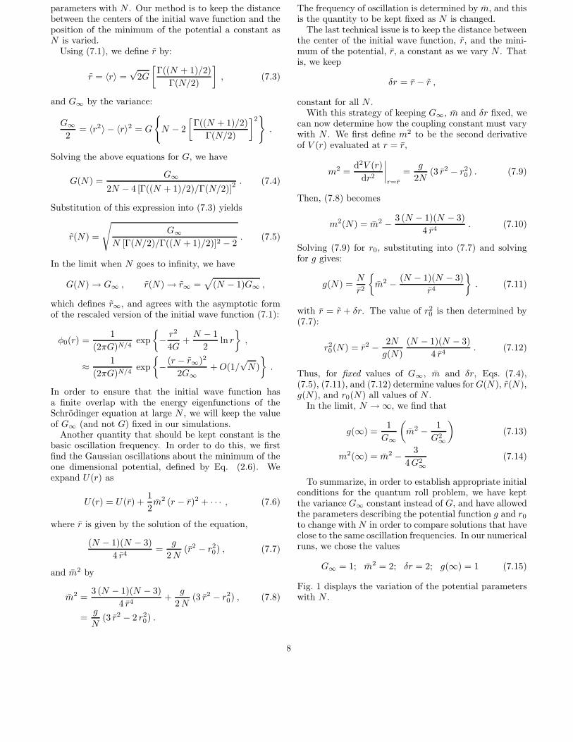
G∞ = 1; m2 = 2; δr = 2; g(∞) = 1 (7.15)

Fig. 1 displays the variation of the potential parameterswith N .

8

0 20 40 60 80 100N

0

0.5

1

1.5

2

2.5

gGm2

y0

FIG. 1. Potential parameters as a function of N .

B. Shifted Gaussian Initial Conditions

The second O(N) invariant initial condition we inves-tigated had a wave function localized in a wave packetnear the center of the valley of the classical potential atr = r0. For N = 1 this would be the standard double-well tunnelling problem; for higher values of N , tunnel-ing is avoided by going around the barrier. Thereforethis initial condition is qualitatively different from theroll problem and provides a different arena for testingapproximations. However, since this initial condition vi-olates the O(N) symmetry of the potential, numericalsolution is at present possible only for very small N .

We take the initial wave function to be a shifted Gaus-sian of the form:

ψ0(x) =1

(2πG)N/4exp

{

−∑

i

(xi − r0/√N)2

4G

}

.

(7.16)

The energy E of this state can be determined fromEq. (6.7) by the substitutions,

Gij → δijG ; qi → r0/√N ; pi → 0 ; Πij → 0 ,

from which we find:

E =N

8G+

g

8N

{

N(N + 2)G2 − 2N Gr20 + r40

}

. (7.17)

On the other hand, the height of the classical potentialbarrier is given by:

Eb =g

8Nr40 . (7.18)

For N = 1, the necessary requirement for tunneling isthat E < Eb.

In the general case (arbitrary N), we have:

M2 =∂2V (r)

∂r2

∣

∣

∣

∣

r0

=g

Nr20 or r20 =

N

gM2 . (7.19)

If the initial state is close to the ground state of a har-monic potential that approximates the potential at thebottom of the well, then the width G of the wave functionis, approximately,

G =1

2√M2

, (7.20)

which can be combined with Eq. (7.17) to give the desiredenergy of the initial state in terms of the values of N andg.

We are interested in initial conditions where the energyper oscillator does not increase as a function of N . Toimplement this we fix M2 = 1, which corresponds toG = 1/2 for the initial width. The barrier height is thengiven by

Eb =N

8g, (7.21)

and the total energy by

E =N + 1

4+N + 2

32g (7.22)

We explored three cases: E = 0.5Eb, E = Eb, andE = 2Eb. For each of these cases, Eqs. (7.21) and(7.22) determine g for each N . In all cases we took

xi(0) = r0/√N , xi = 0, Gij(0) = Gδij , and Gij(0) = 0.

As a consequence, all of the oscillators xi(t) move iden-tically.

VIII. EFFECTIVE POTENTIAL

It is well-known that the static effective potential is notalways a useful guide to the true dynamics of the system(See, e.g., Ref. [4]). Nevertheless, one may seek to gainqualitative insight into some aspects of quantum dynam-ics this way, though care is certainly indicated (See, e.g.,Ref. [19] for the Gaussian effective potential). Indeed,there appears to be an interesting connection with theproperties of the effective potential at next-to-leadingorder and with the corresponding dynamical evolution(discussed in the next section).

The effective potential in the large N approxima-tion has been previously obtained by Root [20] to order1/N ; however, we recalculate it here using our equations.When xi and χ are independent of time, we can ignorethe closed time path ordering and use Fourier transforms,passing the poles by using the Feynman contour. Then,from the action given in (3.3), we find

9

V[1]eff (r, χ) =

Nχ

g

(

µ2 − χ

2

)

+1

2χ r2 (8.1)

+N

2

∫

dk

2πiln[G−1(k)] +

1

2

∫

dk

2πiln[D−1(k)] ,

where χ satisfies the requirement

∂

∂χVeff(r, χ) = 0 . (8.2)

In this section to make contact with Root [20], we haveµ2 = −gr20/(2N) < 0. In order to examine the large Nlimit, we again rescale (2.7) to the y variables. Then forthe Green’s functions, we find:

G−1(k) = −(k2 − χ) ,

D−1(k) = −Ng

−Ny2 G(k) +iN

2

∫

dp

2πG(p) G(k − p)

= −Ng

{

1 − gy2

k2 − χ− g

2√χ

1

k2 − 4χ

}

= −Ng

(k2 −m2+)(k2 −m2

−)

(k2 − 4χ)(k2 − χ),

where m2± = b±

√b2 − c, with

b =5

2χ+

g

2

(

y2 +1

2√χ

)

c = 4χ2 + g

(

4 y2χ+1

2

√χ

)

.

For the Feynman contour, we have∫

dk

2πiln(k2 − χ) =

√χ+ constant terms . (8.3)

Thus the effective potential (8.1) becomes

V[1]eff (y, χ)

N=χ

2

(

y2 − y20

)

− χ2

2 g+

√χ

2(8.4)

+1

2N

(

m+ +m− − 3√χ)

.

The gap equation which determines χ follows from (8.2)

χ =g

2

(

y2 − y20

)

+g(N − 3)

4N√χ

+g

2N

∂(m+ +m−)

∂χ. (8.5)

To leading order in the large N expansion, Eqs. (8.4, 8.5)reduce to the parametric set

V[0]eff (χ)

N=χ2

2g+

√χ

4,

y2(χ) = y20 +

2

gχ− 1

2√χ. (8.6)

Equations (8.4) and (8.5) agree with Root, however heused the leading order expression for χ in (8.6), ratherthan the full χ of (8.5).

There exist two real solutions of Eq. (8.5) for χ withy greater than some minimum value ymin. The next-to-leading order large N effective potential, from Eq. (8.4)is therefore double valued for y > ymin, and does not ex-ist for smaller values of y. The physical solution branchcorresponds to the one that matches on to the leadingorder result; the other branch is an unphysical solution.Since it follows from a Legendre transformation, the ef-fective potential (at any order in 1/N) has to be a convexfunction. The nonexistence of the effective potential aty < ymin implies that no quantum state can be associatedwith the next-to-leading order large N approximation inthis range.

0 1 2 3 4y

0

1

2

3

4

Veff/N

1st orderN = 1N = 5N = 10N = 50

FIG. 2. Veff/N vs y = r/√

N for the leading and next-to-leading order large-N approximation for different values ofN .

In Fig. 2, we plot the physical branch of the effectivepotential as a function of y, for values of N from 1 to100, for the case g = 1 and y0 = 2. For comparison,we also show in this figure the leading order potentialfunction from Eq. (8.6), which is single-valued and finitefor all y. (In contrast to the next-to-leading order casewe can always associate a Gaussian wave function withthe leading order approximation.)

In the case of the Hartree approximation, one can de-fine an “effective potential” as the expectation value ofthe Hamiltonian using the variational wave function (4.2)for static configurations [19,21]. Setting pi(t) = 0 andΠij(t) = 0, and putting

∑

i q2i = r2 and Gij = δijG in

Eqs. (4.6) and (4.8), we find:

V[H]eff (y,G)

N=

1

8G+g

8

(

y2 − y20

)2(8.7)

+ gN + 2

4N

(

y2 +1

2G

)

G− g

4y20 G ,

The value of G is fixed by the requirement that

10

∂ V[H]eff (y,G)

∂G= 0 ,

which gives the gap equation for the Hartree approxima-tion:

χ =g

2(y2 − y2

0) +g

N

(

y2 +1

2χ

)

+g

4√χ, (8.8)

where we have set G = 1/2√χ. Parametric equations for

the Hartree effective potential are then given by:

V[H]eff (χ)

N=

1

2g

(

N

N + 2

)2

χ2 − N

(N + 2)2y20 χ

+N + 4

4(N + 2)

√χ+

g

2(N + 2)2y40

+g

4(N + 2)

y20√χ− g

16N

1

χ(8.9)

y2(χ) =N

N + 2

(

y20 +

2

gχ− 1

2√χ

)

− 1

(N + 2)χ.

Note that in the limit N → ∞, Eq. (8.9) reduces toEq. (8.6), the leading order large N result. Note alsothat the Hartree effective potential is not derived froma Legendre transform and hence is not subject to a con-vexity constraint.

0 1 2 3 4y

0

1

2

3

4

Veff/N

1st orderN = 1N = 5N = 10N = 50

FIG. 3. Veff/N vs y = r/√

N for the Hartree approximationusing the parameters found in Eq. (7.15).

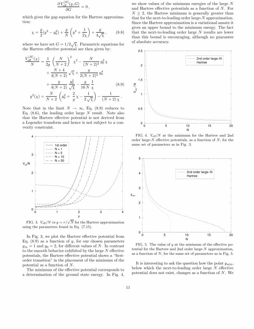
In Fig. 3, we plot the Hartree effective potential fromEq. (8.9) as a function of y, for our chosen parametersg∞ = 1 and y0 = 2, for different values of N . In contrastto the smooth behavior exhibited by the largeN effectivepotentials, the Hartree effective potential shows a “first-order transition” in the placement of the minimum of thepotential as a function of N .

The minimum of the effective potential corresponds toa determination of the ground state energy. In Fig. 4,

we show values of the minimum energies of the large Nand Hartree effective potentials as a function of N . ForN ≥ 2, the Hartree minimum is generally greater thanthat for the next-to-leading order large-N approximation.Since the Hartree approximation is a variational ansatz itgives an upper bound to the minimum energy. The factthat the next-to-leading order large N results are lowerthan this bound is encouraging, although no guaranteeof absolute accuracy.

0 5 10 15 20N

0

0.5

1

1.5

2

2.5

Vm

in /

N

2nd order large−NHartree

FIG. 4. Veff/N at the minimum for the Hartree and 2ndorder large-N effective potentials, as a function of N , for thesame set of parameters as in Fig. 3.

0 5 10 15 20N

0

1

2

3

4

5

ymin

2nd order large−NHartree

FIG. 5. The value of y at the minimum of the effective po-tential for the Hartree and 2nd order large-N approximation,as a function of N , for the same set of parameters as in Fig. 3.

It is interesting to ask the question how the point ymin,below which the next-to-leading order large N effectivepotential does not exist, changes as a function of N . We

11

know that at “infinite N ,” (leading order), ymin = 0but it is important to know how this limit is reached.For instance, is there a finite value of N beyond whichymin = 0? In Fig. 5, we plot ymin as a function of N , forthe Hartree and next-to-leading order large N approxi-mations. As already stated, the Hartree approximationdisplays a first order phase transition between the brokenand unbroken symmetry solutions at N = 6.2, whereasfor the next-to-leading order large N approximation adifferent type of behavior is found: for N ≤ 18.6, ymin

is finite, but for N ≥ 18.6, it hits the origin. Thus forN ≥ 18.6, we can associate a quantum state (though notknown explicitly) with the next-to-leading order approx-imation.

The critical value of N is fixed by the value of χ at thegap equation at the inflection point. If we write the gapequation (8.5) as

f(χ, y2, N) = f0(χ, y2) +

1

Nf1(χ, y

2) = 0 , (8.10)

where

f0(χ, y2) =

g

2(y2 − y2

0) +g

4

1√χ− χ ,

f1(χ, y2) = −3 g

4

1√χ

+g

2

∂(m+ +m−)

∂χ.

Then the critical point is determined by

Nc = −f1(χ, 0)

f0(χ, 0)= −∂f1(χ, 0)/∂χ

∂f0(χ, 0)/∂χ, (8.11)

where χ is given by the solution of this system of equa-tions. For the parameters of Eq. (7.15), we find numer-ically that Nc = 18.60 in excellent agreement with theresults shown in Fig. 5.

IX. NUMERICAL RESULTS

A. Quantum Roll

We begin with a discussion of our results for the quan-tum roll problem. We first examine the short time be-havior, 0 < t < 3, to see if the next-to-leading orderlarge N approximation gives an improvement over theleading order solutions. In Fig. 6, we plot the valuesof 〈r2〉/N from the numerical solution, the leading andnext-to-leading order large-N approximations, and theHartree approximation, for N = 20. The next-to-leadingorder large N approximation is clearly better than theleading order solution, and also better than the Hartreeresults. Similar behavior is seen for other values of N(we also ran N = 50, 80, and 100).

0 1 2 3t

0

1

2

3

< r2 >

/ N

exact1st order large−N2nd order large−NHartree

FIG. 6. 〈r2〉/N for N = 20, for the exact, leading andnext-to-leading order large-N , and Hartree approximationsfor short times.

0 20 40 60 80 100t

0.5

1.5

2.5

3.5

< r2 >

/ N

0 20 40 60 80 100t

1

1.5

2

< r2 >

/ N

FIG. 7. 〈r2〉/N for the exact, leading and next-to-leadingorder large-N , and Hartree approximations for long times.The top figure is for N = 20 while the bottom figure is forN = 100. The labeling conventions are the same as in theprevious figure.

The long time behavior of these approximations is typ-ically of much more interest. We examined behavior overtimes 0 < t < 100 to see how long the approximationsremained viable. Fig. 7 displays 〈r2〉/N for the numeri-

12

cal solution, the leading and next-to-leading order large-N approximations, and the Hartree approximation forN = 20 and 100. The next-to-leading order large-Napproximation for N = 20 blows up at t ∼ 84. Thisinstability is connected to a violation of unitarity in theparticular implementation of this approximation and willbe discussed in greater detail below. In general, at thesemoderate values of N , the approximations track the nu-merical solutions reasonably well though they do get outof phase as time progresses. As N is increased, the phaseerrors are considerably reduced as is apparent in the re-sults for N = 100.

The energy of the next-to-leading order large N andHartree approximations is the same as the exact one, butthe energy of the leading order large N approximationdiffers from it by terms of order 1/N . (This is becausewe need to keep the initial values of the parameters thesame.) To make a comparison between the approxima-tions this difference has to be compensated for; we do thisby rescaling time by a constant multiplicative factor so asto match the last oscillation maxima. This effect is of or-der 1/N . For N = 100, we find that for 0 < t < 100, thenext-to-leading order 1/N approximation is always moreaccurate than the leading order; however, when compar-ing the next-to-leading order with the Hartree, althoughless accurate for t < 50, the Hartree approximation startsbecoming more accurate at t ∼ 50 (however, the errorsare very similar in magnitude, of the order of a few percent).

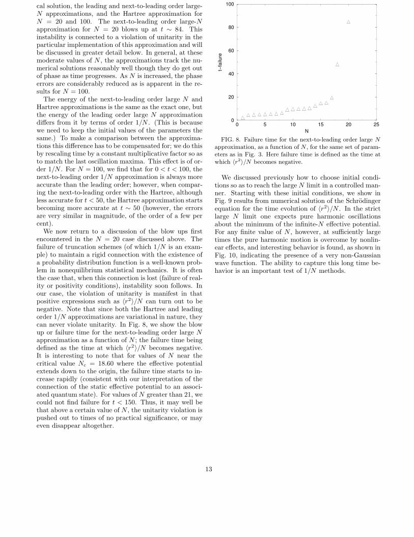
We now return to a discussion of the blow ups firstencountered in the N = 20 case discussed above. Thefailure of truncation schemes (of which 1/N is an exam-ple) to maintain a rigid connection with the existence ofa probability distribution function is a well-known prob-lem in nonequilibrium statistical mechanics. It is oftenthe case that, when this connection is lost (failure of real-ity or positivity conditions), instability soon follows. Inour case, the violation of unitarity is manifest in thatpositive expressions such as 〈r2〉/N can turn out to benegative. Note that since both the Hartree and leadingorder 1/N approximations are variational in nature, theycan never violate unitarity. In Fig. 8, we show the blowup or failure time for the next-to-leading order large Napproximation as a function of N ; the failure time beingdefined as the time at which 〈r2〉/N becomes negative.It is interesting to note that for values of N near thecritical value Nc = 18.60 where the effective potentialextends down to the origin, the failure time starts to in-crease rapidly (consistent with our interpretation of theconnection of the static effective potential to an associ-ated quantum state). For values of N greater than 21, wecould not find failure for t < 150. Thus, it may well bethat above a certain value of N , the unitarity violation ispushed out to times of no practical significance, or mayeven disappear altogether.

0 5 10 15 20 25N

0

20

40

60

80

100

t−fa

ilure

FIG. 8. Failure time for the next-to-leading order large Napproximation, as a function of N , for the same set of param-eters as in Fig. 3. Here failure time is defined as the time atwhich 〈r2〉/N becomes negative.

We discussed previously how to choose initial condi-tions so as to reach the largeN limit in a controlled man-ner. Starting with these initial conditions, we show inFig. 9 results from numerical solution of the Schrodingerequation for the time evolution of 〈r2〉/N . In the strictlarge N limit one expects pure harmonic oscillationsabout the minimum of the infinite-N effective potential.For any finite value of N , however, at sufficiently largetimes the pure harmonic motion is overcome by nonlin-ear effects, and interesting behavior is found, as shown inFig. 10, indicating the presence of a very non-Gaussianwave function. The ability to capture this long time be-havior is an important test of 1/N methods.

13

0 20 40 60 80 100t

0

5

10

15

< r2 >

0 20 40 60 80 100t

1

2

3

4

5

6

< r2 >

0 20 40 60 80 100t

1

2

3

4

5

< r2 >

0 20 40 60 80 100t

1

2

3

4

< r2 >

FIG. 9. Exact solutions for 〈r2〉/N as a function of time.From top to bottom, N = 1, 5, 10, and 20.

0 100 200 300 400 500t

0

5

10

15

<r2>/N

0 100 200 300 400 500t

1

2

3

4

5

<r2>/N

FIG. 10. Very long-time behavior of the exact results for〈r2〉/N for 0 ≤ t ≤ 500. The top figure is for N = 1 and thebottom figure for N = 10.

In order to test whether Hartree or the next-to-leadingorder approximation incorporate nonlinearities correctlyso as to capture the late time modulation behavior, weran a comparison against the numerical results for N =21, the results being displayed in Fig. (11). It is clearthat both approximations do not give satisfactory results.This provides additional motivation for the developmentof alternative 1/N expansions which would incorporateselective resummations in order to reduce the coefficientof the error term at late times.

0 25 50 75 100 125 150t

0.5

1.5

2.5

3.5

< r2 >

/ N

exact2nd orderHartree

FIG. 11. 〈r2〉/N for N = 21, for the exact, next-to-leadingorder large N , and Hartree approximations for late times.

14

B. Shifted Gaussian Initial Conditions

We now discuss the time evolution of a quantum statehaving an initial wave function given by Eq. (7.16). Forthis problem, because of the lack of symmetry, exact so-lutions were only obtained for N ≤ 2. For N = 1, de-pending on whether the energy is above or below thebarrier height, one observes either slow tunneling withrapid oscillations in one well, or slower oscillation in thecomplete range. At these low values of N , the large-Nexpansion breaks down quickly, as in the quantum roll,but even here at N = 1, the 1/N corrections improve theshort time accuracy of q(t).

A more relevant comparison is to consider larger valuesof N at which the approximations have a better chanceof capturing the exact behavior. In the next figure, wecompare the Hartree with the leading and next-to-leadingorder large-N approximation for q(t), at N = 50. Fig. 12displays the results for a run with E > Eb using theequal time Green’s function approximation (see Sec. V)method for obtaining the Hartree results. Unlike the sit-uation for the roll initial condition where the Hartree andnext-to-leading order largeN results are not dramaticallydifferent, here the qualitative behavior is quite dissimilar(whereas the Hartree and leading order results are in factvery close).

0 20 40 60 80 100t

−2

−1

0

1

2

q(t)

ETGF1st order2nd order

FIG. 12. Plot of q(t) vs t for E > Eb with N = 50.

X. CONCLUSIONS

Testing the 1/N approximation in quantum mechanicshas already enabled us to arrive at some useful conclu-sions. In order to interpret our results, it is important tokeep in mind that 1/N approximations are a form of re-summed perturbation theory and are therefore only validat weak coupling. Thus for couplings of order unity, it isunrealistic to expect the approximation to give good re-sults for small values of N . Our results have shown that

at sufficiently large N the next-to-leading order approx-imation is a clear improvement over the leading orderapproximation, however, at late times this approxima-tion (as well as Hartree) fails to capture the nonlineareffects that lead to nontrivial amplitude modulation ofthe radial oscillations in the quantum roll problem.

We have noted the presence of a finite-time breakdownin the evolution given by the next-to-leading order ap-proximation. This result is related to the fact that thelarge N expansion for the expectation values does notnecessarily correspond to a positive semi-definite densitymatrix when truncated at any finite order in 1/N . (Atlowest order, the 1/N approximation is equivalent to aGaussian variational ansatz for the density matrix anddoes not have this problem.) This last aspect is alreadyclear even in static situations such as the lack of a real ef-fective potential for allN in the next-to-leading order ap-proximation. This type of finite-time breakdown inducedby unitarity/positivity violation has also been noted insimulations of quantum systems where the coupled equaltimes Green’s function approach was truncated at fourthorder [22] or where high order cumulant expansion meth-ods were used [23].

Two aspects of this breakdown deserve further men-tion: First, the time at which breakdown occurs appearsto be strongly connected with the behavior of the effec-tive potential. For values of N not very much bigger thanthe critical value Nc (beyond which the effective poten-tial exits over the entire range of y), the breakdown timeincreases extremely steeply and may even be pushed totimes long enough to be no longer an obstacle to prac-tical calculations ( this still needs to be demonstrated).Second, it is important to point out that avoiding thebreakdown via a partial resummation does not automat-ically guarantee better late time accuracy (or conver-gence) since such a scheme is also only next-to-leadingorder accurate. However, it will help in the sense that onemay carry out simulations at smaller values of N , thusmaking it easier to compare against the late-time numer-ical solutions of the corresponding Schrodinger equation.

One possible way of correcting the problem of a man-ifestly positive operator such as 〈r2〉 becoming negativeis to solve for the full Green’s function Gij(t, t

′):

Gij(t, t′) = Gij(t, t

′) (10.1)

−∑

k,l

∫

C

dt1

∫

C

dt2Gik(t, t1) Σkl(t1, t2)Glj(t2, t′) ,

rather than the next-to-leading order one as in (3.7).This equation is the exact equation one obtains by vary-ing the effective action and it contains terms of all ordersin 1/N (thus, strictly speaking, one is no longer truncat-ing at some fixed order).

However, just making this correction does not increasethe time period during which the approximation is ac-curate. In order to extend the accuracy of the 1/N ap-proximation to late times, it appears necessary to use

15

a more robust approximation based on the Schwinger-Dyson equations. Several approximations of this sort arepossible, which may both cure the positivity problem aswell as lead to accurate results at late times. These willbe discussed separately [24].

XI. ACKNOWLEDGEMENTS

The authors acknowledge helpful conversations withLuis Bettencourt, Yuval Kluger, and Emil Mottola. S.H.acknowledges stimulating discussions with Larry Yaffe.The work of B.M. and J.F.D. at UNH is supported in partby the U.S. Department of Energy under grant DE-FG02-88ER40410. B.M. and J.F.D thank the Theory Group(T-8) at LANL and the Institute for Nuclear Theory atthe University of Washington for hospitality during thecourse of this work. F.C. would like to thank the PhysicsDepartment at Yale University for their hospitality wheresome of this research was carried out.

[1] H. E. Stanley, Phys. Rev. 176, 718 (1968); K. Wilson,Phys. Rev. D 7, 2911 (1973)

[2] S. Coleman, R. Jackiw and H. D. Politzer, Phys. Rev. D7, 2911 (1973).

[3] F. Cooper, Y. Kluger, E. Mottola, and J. P. Paz, Phys.Rev. D 51, 2377 (1995);M. A. Lampert, J .F. Dawson, and F. Cooper, ibid 54,2213 (1996); hep-th/9603068.

[4] F. Cooper, S. Habib, Y. Kluger, and E. Mottola, Phys.Rev. D 55, 6471 (1997); D. Boyanovsky, H. J. de Vega,R. Holman, D.-S. Lee, and A. Singh, Phys. Rev. D 51,4419 (1995).

[5] A. H. Guth and S.-Y. Pi, Phys. Rev. D 32, 1899 (1985);F. Cooper, S-Y. Pi and P. Stancioff, ibid 34, 383 (1986);G.J Cheetham and E.J. Copeland, ibid 53, 4125 (1996);gr-qc/9503043.

[6] N. Turok and D. N. Spergel, Phys. Rev. Lett. /bf 66,3093 (1991); A. H. Jaffe, Physical Review D /bf 49, 3893(1994); R. Durrer, M. Kunz, and A. Melchiorri, ibid 59,123005 (1999).

[7] F. Cooper, S. Habib, Y. Kluger, E. Mottola, J. P. Paz,and P. R. Anderson, Phys. Rev. D 50, 2848 (1994); hep-ph/9405352.

[8] F. Cooper, J. F. Dawson, S. Habib, Y. Klugerand D. Meredith, Physica D83, 74 (1995); quant-ph/9610013.

[9] B. Mihaila, J.F. Dawson, and F. Cooper, Phys. Rev. D56, 5400 (1997); hep-ph/9705354.

[10] R. H. Kraichnan, Phys. Rev. Lett. 78, 4922 (1997);P. J. Channell (private communication).

[11] J.-P. Blaizot and G. Ripka, Quantum Theory of FiniteSystems (MIT press, Cambridge, MA; 1986), p. 156.

[12] M. R. Hermann and J. A. Fleck, Jr., Phys. Rev. A 38,6000 (1988).

[13] B. Mihaila and I. Mihaila, physics/9901005.[14] P. A. M. Dirac, Appendix to the Russian edition of The

Principles of Wave Mechanics, as cited by Ia. I. Frenkel,Wave Mechanics, Advanced General Theory (ClarendonPress, Oxford, 1934), pp. 253, 436. Pattanayak andSchieve [25] point out that the reference often quoted,P. A. M. Dirac, Proc. Cambridge Philos. Soc. 26, 376(1930), does not contain this equation!

[15] R. Jackiw and A. Kerman, Phys. Lett. 71A, 158 (1979);F. Cooper, S-Y. Pi and P. Stancioff, Phys. Rev. D 34,383 (1986).

[16] F. Cooper, J. F. Dawson, S. Habib, and R. D. Ryne,Phys. Rev. E 57, 1489 (1996); quant-ph/9610013.

[17] G. F. Mazenko, Phys. Rev. Lett 54, 2163 (1985);F. Cooper and E. Mottola, Phys. Rev. D 36, 3114 (1987).

[18] C. Wetterich, Phys. Rev. Lett. 78, 3598 (1997);D. Boyanovsky, F. Cooper, H. J. de Vega, and P. Sodano,Phys. Rev. D 58, 25007 (1998); hep-ph/9802277.

[19] P. M. Stevenson, Phys. Rev. D 30, 1712 (1984)[20] R. G. Root, Phys. Rev. D 10, 3322 (1974).[21] P.M. Stevenson, B. Alles, and R. Tarrach, Phys. Rev. D

35, 2407 (1987).[22] L. M. A. Bettencourt (private communication) and

L. M. A. Bettencourt and F. Cooper (In preparation).[23] S. Habib and K. Shizume (unpublished).[24] B. Mihaila, J. F. Dawson, and F. Cooper, (in progress).[25] A. K. Pattanayak and W. C. Schieve, Phys. Rev. E 50,

3601 (1994).

16