Evolution of the Earth

Chapter 4

MAIN TOPICS:ROCK FACIES

RELATIVE TIMEGEOLOGIC TIME SCALE

RELATIVE GEOLOGIC TIME

• As geologic thought progressed in the early 1800’s it became necessary to classify and organize material (fossils) and concepts (maps)) in a more orderly and manageable form.

• In 1835 Adam Sedgwick and Roderick Murchison proposed formal names for the entire European stratigraphic succession.

• Eras (Paleozoic, Mesozoic, Cenozoic)• Periods (Vendian, Cambrian, Ordovician, etc.)• Based solely on fossils (e.g. fossil life spans)

• Based on fossils and Steno’s Laws

GEOLOGIC TIME SCALE ORIGINATED IN ENGLAND, FRANCE, GERMANY

GEOLOGIC TIME SCALE

• PALEOZOIC ERA (383 My)– LOWER PALEOZOIC

• CAMBRIAN (Cambria)• ORDOVICIAN• SILURIAN (Silures)

– UPPER PALEOZOIC• DEVONIAN (Devonshire)• CARBONIFEROUS (coal-bearing)

– MISSISSIPPIAN (N. America)– PENNSYLVANIAN (N. America)

• PERMIAN

• MESOZOIC ERA (183 My)– TRIASSIC (Trias, Germany)– JURASSIC (Jura Mtns.)– CRETACEOUS

• CENOZOIC ERA (66 My) (cont.)

Fig. 4.2

Geology of Northwestern Europe where much of the geologic time scale was developed. Note the unconformities and lateral extend of major rock units.

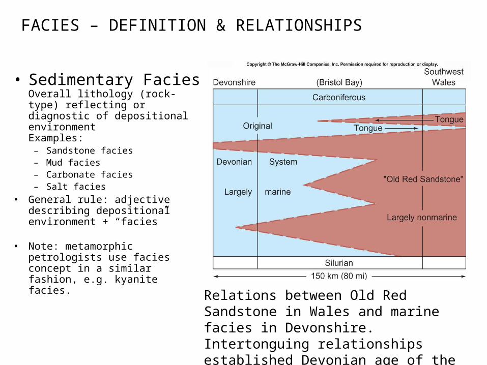
FACIES – DEFINITION & RELATIONSHIPS

• Sedimentary FaciesOverall lithology (rock-type) reflecting or diagnostic of depositional environmentExamples:

– Sandstone facies– Mud facies– Carbonate facies– Salt facies

• General rule: adjective describing depositional environment + “facies”

• Note: metamorphic petrologists use facies concept in a similar fashion, e.g. kyanite facies. Relations between Old Red Sandstone in Wales

and marine facies in Devonshire. Intertonguing relationships established Devonian age of the Old Red Sandstone.

Fig. 4.4

Source of nomenclature feud between Sedgwick and Murchinson. As their field areas converged it became apparent that each has included the same rocks in his own classification. Sedgwicks’ top of Cambrian overlapped Murchinson’s lower Silurian. After their deaths, the dispute was resolved by naming a new system, the Ordovician.

Fig. 4.5

Cross-section across Scotland showing superposition, cross-cutting and included-fragment relationships. What is the sequence of events here?

Included fragments: Any rock represented by frag ments in another rock must be older than the host rock.

Cross-cutting relationships: Any igneous rock or any fault must be younger that the rocks it cross cuts.

Relative Geologic Time

Fig. 4.5

Sequence of events here: the primitive and transition rocks were (1) folded, intruded by granites, uplifted and deeply eroded before deposition of Old Red Sandstone on unconformity surface. This was followed by injection of dikes and sills.

Relative Geologic Time

Fig. 4.6ROCK UNITS (LEFT) AND TIME CHART (RIGHT)

Observed rock unit (left) and interpreted time chart on right. Note hiatus corresponding to unconformities. (Hiatus is a time of non-deposition and/or erosion.)

Fig. 4.7

FORMATION – a mappable unit either in the field or by well logsA GROUP consists of 2 or more FORMATIONS.

A formation is the basic rock unit in geology. IT IS NOT A TIME UNIT. It is defined by its properties: type (sandstone, limestone, etc. e.g. (Bell Shale), color (Brown Niagrian), texture, geometry. The choice is fairly obvious in A, but more difficult in B. In B and C the choice of subdivisions is somewhat arbitrary.

Fig. 4.8

Lavoisier’s 1789 diagram showing relationships between littoral gravels (near-shore) and pelagic (mud, off-shore) facies illustrating transgression and regression. Lavoisier recognized that gravel can only be moved in a high-energy environment, such as the near-shore where braking waves provide energy. He also recognized that distinctive organisms inhabit each environment and that rise and fall of sea-level would cause the sediments to migrate: shoreward with rising sea-level and seaward with falling sea-level.

Lateral Relationships: different facies, same time

Depositional Environments and Sedimentray Facies

• Lateral variations of strata not fully appreciated until 1838

• Facies concept relates sediments to their depositional environment

Fig. 4.9

Block diagramshowing proximal (near source) and distal (distant from source) facies relationships in a shoreline environment. The source area is the uplifted “island” which is supplying sediment (gravel, sand, mud in that order) as it erodes)

[Note: diagram OK for clastic (clasts = particles) sediments, but not carbonates (precipitates).]

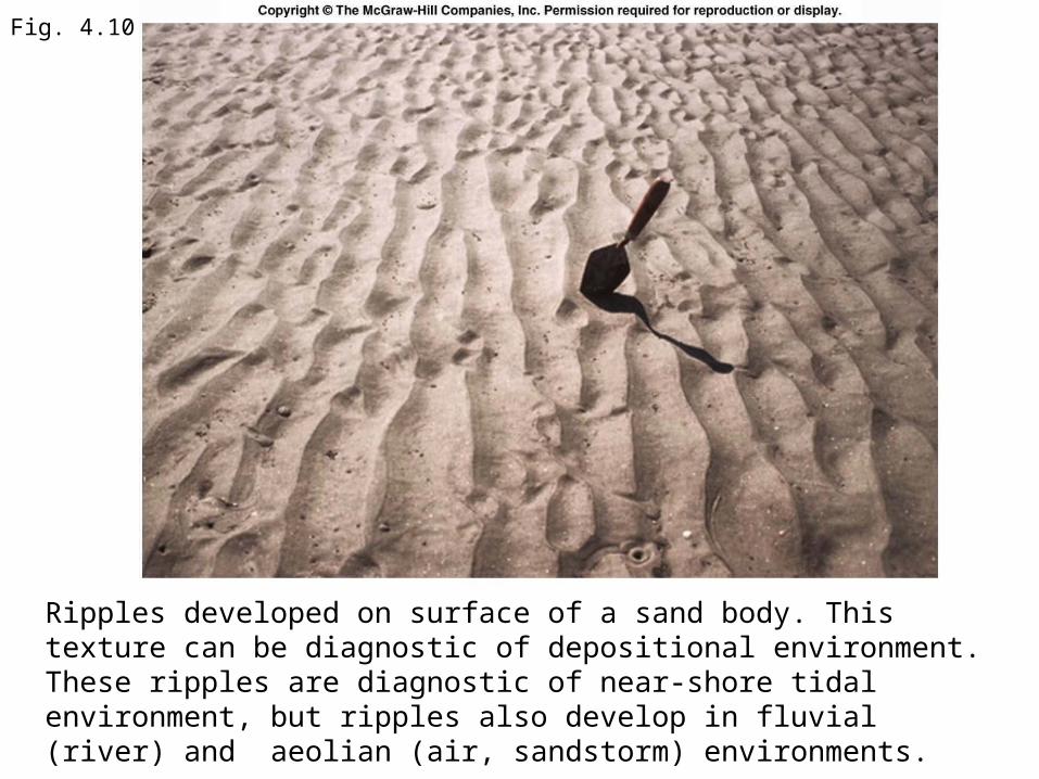
Fig. 4.10

Ripples developed on surface of a sand body. This texture can be diagnostic of depositional environment. These ripples are diagnostic of near-shore tidal environment, but ripples also develop in fluvial (river) and aeolian (air, sandstorm) environments.

Fig. 4.11a

Illustration of restored facies map for Devonian of Europe. Note how this illustrates Steno’s law of lateral continuity. Also, how extensive the different depositional environments are. Lines refer to cross-sections in following diagrams.

Fig. 4.11b

Time-stratigraphic chart showing time gaps represented by unconformities in B

Restored cross section showing facies, thicknesses & unconformities

Fig. 4.12

Recent marine transgression (sea-level rise) on Netherlands coast showing landward shift of facies. Absolute ages from radiocarbon dating. Note shift in facies patterns as sea transgresses. Note how time-lines cross facies boundaries.

Two basic types of facies patterns: transgressive and regressive

Fig. 4.13

Example of regression (falling sea level) caused by glacial uplift rebound) during the past 14,000 years. Notice how unconformity follows the retreating sea level. Also note how the sedimentary (facies) patterns are same for preceding figure (sea-level rise); as expected since sediments were deposited during sea-level rise. Where does eroded material go when sea-level falls? (It is deposited locally, but note that most of the material now above sea-level simply remains in place as “erosional highs”.

Note we can have simultaneous regression and transgression in different parts of the world (see previous figure) due to different geologic agents acting in different places e.g. sea level rise and rebound. What happens when rebound stops? When sea level stops rising?

Fig. 4.14

Contrasting effects of sea level rise on shallow (Bangladesh) versus steep (Vancouver) coastlines. The shift in shoreline can be 10s to 100s of miles in shallow shore lines compared to may be only 10s of feet in steep areas. Present day sea level rise is thought to be due to upwarping of ocean basins.

Fig. 4.15

Advance of Tigris-Euphrates river delta (175 km into Arabian Gulf) during the past 3000 years in spite of a worldwide rise in sea level of abut 4 meters during this time. Rapid sedimentation is the cause, perhaps induced by human agricultural practices? Note calculated average sea-level rise is about 4 mm/yr.

Fig. 1.8

Fertile Crescent region of Middle East. Note position of Tigris-Euphrates River delta.

Tigris and Euphrates River Delta

This image is a Landsat scene of the mouth of the fabled Tigris and Euphrates Rivers as it empties through a delta into the Persian Gulf in southeastern Iraq. Those rivers meet into a single channel, the al Arab, in the swamplands in the upper left of the image. The Rivers Karun (top center) and Jarrahi (right center) are both in western Iran. The lower left corner is a barren desert, with sand dunes. Several black plumes of smoke emanate from the burning oil fields in Kuwait.

Correlation using three different index fossils. A single fossil zone is shown in blue. Note that range and maximum development (indicated by pattern width) vary from place to place.

Fig. 4.17

Significance of differentrates of evolution and changes inenvironment (due to transgression). Thebrachiopod evolved slowly and stayed in/on sand facies. It is a poor index fossil. The cephalopods evolved rapidly and are free swimmers. They were changing and widely distributed and thus excellent index fossils.

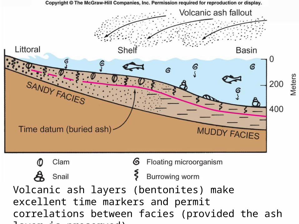
Fig. 4.18

Volcanic ash layers (bentonites) make excellent time markers and permit correlations between facies (provided the ash layer is preserved).

Fig. 4.19

Conodont.

A conodont is a preserved bony part of an extinct eel. It evolved rapidly and is widely distributed across many facies types. They are excellent index fossils and can be used to determine maximum burial temperatures as well. Conodont specialists were once highly sought after by oil companies.

Fig. 4.20

Block diagram showing relationships between formations and index fossils. Fossil zone C shows that Formation 3 is synchronous everywhere, but zones 1 and 2 vary in age. How can you tell?

Fig. 4.21

Fig. 4.22

SLOSS SEQUENCES (6)

Six unconformity bounded sequences from which a world-wide sea-level fluctuation curve has been inferred (the “Vail” curve).

Note two maxima (highs) at about 500 and 75 million years and three minima at 600, 200 and the present.

Max +350 to -150 m above and below present.

Fig. 4.23

Effects of sea level change on sediment accumulation and unconformities at a continental margin.

Additional Relative Time Scales

• In addition to index fossils, there are several other ways to determine relative time:

• The sequence unconformities just discussed

• Magnetic reversals

• Isotope geochemistry e.g. strontium isotopes work pretty well back to end ot Miocene.

Fig. 4.24

Magnetic reversals over past 80 million years. These reversals are recorded in sediments and can be used for relative time dating.

Fig. 4.25

Graph of depositional rates of a hypothetical sequence of strata. The continuous average rate of deposition is computed by dividing the strata thickness by the time interval. The actual rate accounts for changes in rate of deposition as well as for erosional events.

EARLY DEVONIAN 400 MY

• 2 global hemisphere views one centered on North America and the other centered on the Tethys-Indian Ocean region. A global mollewide projection with labels and 1st-order tectonic elements shows the whole Earth for the Early Devonian.

http://jan.ucc.nau.edu/~rcb7/paleogeographic.html

PALEO-RECONSTRUCTION

http://jan.ucc.nau.edu/~rcb7/paleogeographic.html

• 2 global hemisphere views one centered on North America and the other centered on the Tethys-Indian Ocean region. A global mollewide projection with labels and 1st-order tectonic elements shows the whole Earth for the Late Devonian.

http://jan.ucc.nau.edu/~rcb7/paleogeographic.html

PALEO-RECONSTRUCTION

LATE DEVONIAN 370 MY

http://jan.ucc.nau.edu/~rcb7/paleogeographic.html