Evolution of quantum superpositions in open environments: Quantum trajectories, jumps, and localization in phase space

PHYSICAL REVIEW A VOLUME 50, NUMBER 3 SEPTEMBER 1994

Evolution o& quantum superpositions in open environments:Quantum trajectories, jumps, and localization in phase space

B.M. Garraway and P. L. Knight

(Received 29 April 1994j

The decay of coherence when a quantum system interacts with a much larger environment is usually

described by a master equation for the system reduced density matrix and emphasizes the evolution of an

entire ensemble. We consider two methods that have been developed recently to simulate the evolution

of single realizations. Quantum-state diff'usion involves both diffusion, where the individual quantum

trajectory fluctuates through a %iener process deriving from the environment, and localization to a

coherent state, an eigenstate of the relevant Lindblad operator describing the coupling of the system tothe environment. %e demonstrate the localization process for different initial states and utilize the

Wigner function to depict this localization in phase space. We concentrate on quantum states that canbe expressed as a superposition of appropriate coherent states. For an initial superposition of two

coherent states (a Schrodinger "cat"), one of the two components will dominate the evolution. For ini-

tial Fock states, which can be described as a continuous superposition of coherent states on a ring, locali-

zation takes place when one coherent state is selected from that ring where each component has nearly

the same energy as the original Fock state. %e also consider the localization from a nonclassical

squeezed ground state, which can be expressed as a superposition of coherent states along a line in phase

space; The second simulation method considered is the state vector Monte Carlo, or "quantum jump,"

approach, which relates to the direct counting of decay quanta. In the case of an initial Schrodinger"cat," we find that when no quantum is detected the "cat" shrinks, but when a quantum is detected, the

Schrodinger "cat" "jumps" from one type of "cat" to another with different internal phase. For an ini-

tial squeezed state we show how quantum jumps lead to individual realizations which are superpositionsof two squeezed states.

PACS number(s): 42.50.Lc, 42.50.Dv

I. INTRODUCTION

Closed quantum systems evolving entirely through re-versible Hermitian dynamics, are frequently employed inquantum dynamics, with the Jaynes-Cummings model ofa single two-level atom interacting with a single quantumfield mode being perhaps the best known example [1]. Insuch idealizations, subsystems become entangled andcoherences created. In reality, no quantum system canever be entirely isolated from its environment and its dy-namics need to be supplemented to recognize the irrever-sible decay of energy and coherences characteristic ofopen systems [2]. A method which is widely adopted todescribe such behavior is the master equation for the re-duced density operator (having traced out the degrees offreedom of the larger environment) with the system-environment coupling treated in the Born-Markov ap-proximation [3]. This method describes the evolution ofan ensemble of realizations of the quantum system andshows that coherences (especially those characterizingmacroscopic superpositions) decay much faster than thesystem energy [4—6]. This ensemble approach is wellsuited for problems such as those involving many atomsinteracting with a radiation field. But it does not easilyaddress the question of how an individual member of anensemble evolves in a dissipative environment, eventhough this issue is accessible to experiment. For exam-ple, the quantum jumps in the Auorescence of a single

three-level ion undergoing intermittent shelving in ametastable state [7,8] are well known. Similarly, quan-tum jumps in the photon excitation number of a singlemode of a high-Q cavity have been studied theoretically[9,10] and experimentally [11]. Recently, methods to de-scribe the evolution of single quantum systems interact-ing with an open environment have been developed fortheir intrinsic interest [8,12—27] and for practical compu-tational reasons ever when an ensemble is of primary in-

terest [28—34].In this paper we address the question of how a single

realization of a superposition of radiation field statesevolves in a dissipative environment. That is, we examinethe evolution of prepared quantum superpositions condi-tioned by measurements we are able to make on the decayproducts of the dissipation, with the record of such con-ditioned measurements being particular to that realiza-tion. The evolution of such a superposition will of coursedepend on the precise measurement scheme adopted: forradiation fields one may imagine quadrature measure-ments of field variables as one such scheme or direct pho-ton counting as another. All hinge ultimately on thecounting of quanta. The state vector Monte Carlomethod [12,13] has been developed to simulate the evolu-tion of a single realization conditioned by the observationof decay quanta and centers on quantum jumps rejectingthe information gained from such observations. It in-volves a continuous evolution which is interrupted by

1050-2947/94/50(3)/2548(16)/$06. 00 1994 The American Physical Society

50 EVOLUTION OF QUANTUM SUPERPOSITIONS IN OPEN. . . 2549

"instantaneous" jumps as the state vector is conditioned

by information gained from the register of counts. Theother method commonly adopted involves both aquantum-state diffusion [15], where the individual quan-tum trajectory Auctuates through a Wiener process deriv-

ing from the environment, and localization to a coherentstate [19],an eigenstate of the relevant Lindblad operatorR describing the coupling of the system to the environ-ment [35]. For example, in one-photon decay R is the an-

nihilation operator a for the field mode, whereas in two-photon decay R ~a [22,23] and in atomic spontaneousemission decay R ~0. , the Pauli lowering operator forthe atomic excitation. Milburn and Wiseman, and others[12,14,36,37] have related these two simulation schemes,the Monte Carlo wave function method, and thequantum-state diffusion method, to specific measurementschemes: the quantum-jump method to continuous directcounting of decay quanta and the quantum-state diffusionmethod to a heterodyne measurement of oscillation am-

plitudes. Each has a distinct and characteristic evolutionfor single realizations. But we should stress that theaverage over a family of very many realizations generatesprecisely the ensemble evolution predicted by thedensity-matrix treatment, quite independent of the partic-ular choice of conditioning. That is, there are manyequivalent ways of "unraveling" the master equation,each appropriate to a particular choice of conditioning[12]. The simulation of these individual realizations gen-erates a family of trajectories which, independent of thekind of conditioning used, average to the usual density-matrix predictions of decoherence for the ensemble [4].

In the approach adopted here, the quantum jumps areobtained from conventional quantum mechanics by in-clusion of the effects of the larger environment in whichthe quantum system is embedded. Some authors have ex-amined modifications of the Schrodinger dynamics goingbeyond conventional quantum mechanics by invoking"intrinsic" mechanisms for decoherence [38]. We haveshown elsewhere [39] that for some cases these intrinsicmechanisms act as dephasing rather than dissipativeinfluences in quantum optics. We also wish to stress thatwe adopt the conventional measurement interpretation ofquantum-state diffusion even though quantum-statediffusion has its origins in stochastic quantum mechanics[40].

In Sec. II we first review the treatment of dissipationusing the standard master equation form and then we re-view both the quantum-jurnp and quantum-state diffusionmethods. In Sec. III we explore cases of quantum-statediffusion in more detail and then in Sec. IV we contrastthe examples of quantum-state diffusion with the corre-sponding quantum-jump simulations. Section V con-cludes this paper.

II. THE MASTER EQUATIONAND THE SIMULATION METHODS

A. Density-matrix approach

One standard method for dealing with dissipative prob-lems is the density-matrix approach [41] where the sys-

tern of interest (a cavity field mode or a single two-level

atom, for example) interacts with a reservoir describingthe infinite number of degrees of freedom responsible forthe irreversible decay. The density matrix describes alack of precise knowledge about a quantum system. Inthe current context the lack of knowledge arises from thederivation of the (quantum optics) master equation forthe reduced density operator describing the system alone,which involves a trace over the reservoir and results instatistical uncertainty in the state vector.

The system on which we focus in this paper consistssimply of a single mode of the radiation field which byvirtue of its coupling to some kind of reservoir undergoesdissipation or a loss of energy. As stated in the Introduc-tion, we envisage a mode of the electromagnetic field, butthe arguments apply equally to any kind of quantized os-cillator. For simplicity, we consider a zero-temperaturereservoir, so that the relaxation proceeds purely by spon-taneous rather than stimulated transitions. It is straight-forward to generalize the argument to include finite-temperature effects [16]. The standard treatment resultsin the master equation for the density of matrix

when the rotating-wave approximation has been made.There is no Hamiltonian term describing the free (nondis-sipative) evolution because we consider only the decay ofa prepared quantum state and because the density matrix

p is transformed to the interaction representation. How-ever, coherent couplings can be included in a straightfor-ward way. As usual, & and & describe the emission andabsorption of photons and the symbol ~ gives the meanloss rate of energy from the mode.

B. Formalism of quantum-jump simulations

The simulation methods deal with ensembles of purestates where the quantum system of interest decays into areservoir irreversibly: measurement of the decay prod-ucts condition the evolution of the state vector describingthat particular realization. The simulation proceeds byexamining the evolution of single realizations whose stateis conditioned by the gain in knowledge acquired throughthe measurement process. In this way we can dispensewith the need to use the density matrix. The evolution ofthe entire ensemble is then obtained from an appropriateaveraging process. Because photon emission events arerandom and uncontrollable this generally results in a sto-chastic evolution of the state vector in time. In a corn-puter simulation we recreate the history of measurementswith the correct likeliness in time. To obtain results thatare comparable to those obtained from the master equa-tion (1) we average over an ensemble of state vectors. Inthe case of such a monitored system the decay rate sc cor-responds to the mean absorption rate of photons by thequantum photon counter. For the purposes of the theorywe assume a photon counter which is perfectly efficient,but which takes time to absorb the energy of the quan-tum state that it is measuring. The theory can be extend-ed to detectors with finite efficiency. Simulation methods

2550 B.M. GARRAWAY AND P. L. KNIGHT 50

&&g(r)l&'&11t(r) &

(3)

This is sometimes known as a quantum measurement ofthe second kind [42]. If there is a null result we propa-gate the state vector over 5t with the non-HermitianHamiltonian

such as those we discuss here are motivated by more thana need to describe specific approaches to measurement.The methods can be used as simply a practical way of ap-proximating the solution of a master equation of the typegiven in Eq. (1), especially when the dimensionality of thesystem precludes the use of density matrices usingmodest-size coInputers.

The quantum jump simulation of histories can be car-ried out in the following way. We represent the state vec-tor ~ij'l(t ) ) as a complex vector within a computer model.Time is discretized in intervals of, say, 5t. At any time r

the probability for the detection of a photon in a short in-terval 5t is simply given by

aP=~&y(r)~a'a~y(r))5r . (2)

This is evaluated and compared to a random nu~ber todetermine whether or not the detection will take place atthe given time in the simulation. If a decay quantum isdetected, the state vector is modified by a quantum jump;we apply the operator d and renormalize dP„,(t ) = —~& q(r )iraq(r ) &P„,(r ) . (7)

Now we consider the unnormalized state vector ttt(t)),which undergoes evolution with H,s (Note .that all un-

normalized state vectors are denoted with a tilde in thispaper). During the period when there is no jump its timeevolution is

spersed with the jumps. The factors v t( are includedwith each of the jumps so that the square of the normali-zation factor N (r ) represents the conditional probabilityof the whole sequence if jumps are only to be found attimes t . We can renormalize at the end of this sequencebecause we are supposing now that the times t areknown; they do not have to be determined from a nor-malized probability.

This interpretation of N (t) and the consistency ofH, s and the jump (3) can be illustrated in the followingway. We suppose there has been no jump to a time t andwe let the symbol P„J(t) stand for the probability of this.So at a later time t +5t we may use elementary probabili-ty theory to write

P„,(r+5i)=P„,(t)[1—bP] .

If we now insert the jump probability from Eq. (3) andtake the limit 5t ~0 we obtain the differential equation

H~fr 2l IC(l 0 (4)

—I y(r ) &

= —iH ly(t ) &= ——"|2ly(r ) &,

dt '~ 2

The state vector must also be renormalized in this casebecause H,z is non-Hermitian. In this version of thequantuIn jump method the state vector must be renor-malized at every time step to ensure that the transitionprobabilities (2} are calculated correctly. In a differentversion of the method [29,31,12,21,32] one calculates astochastic time interval to the next jump [43] and so lessrenormalization is required. In general the two steps inthe simulation are entirely equivalent to (1) when ensem-ble averaged as, for example, shown in [12,13,23].

We consider next the form of the state that emergesafter m jumps, or detection events, and the probabilitythat m jumps take place during an individual run. Wehave seen that the general form of the state vector evolu-tion consists of the smooth evolution of Eq. (4) interrupt-ed with the jumps of Eq. (3). Given a sequence of jumpsat times t i, t 2 t 3 . , t we analytically calculate thestate vector that results. This is found to be a state vec-tor that is conditional on the measurement process: us-ing the rules above one finds that

~ ~( ) )1 —8tt(t —t )/2~— —8 (t —ttt)/2

N (t)

as found in Eq. (5). The relation between ~)t((t)) andittp(t)) is simply that

& & y(r)ly(r))(9)

and since from Eq. (8} the square of the normalization& tt)( t ) i (I)( t ) ) obeys the equation

we see that it obeys the same equation as P„J( t ) and thus,since it has the same initial condition, P„(t) and&P(i)i(I)(i) ) are identical.

We have now justified Eq. (5) and having identified[N (t)] with the conditional probability we proceed tosimplify the equation by placing the operators 8 together:

ttt)

m /2

i y( r ) ) —( ttt /2g m —ttt8 /2i

—y( () ) )

N (r))m /2 —ttt. /2 ttr8/2gmiy(0) )—

N (t)

[&p(r ) p(r ) &]= 8&tt)(r )l &l,ttt(—r ) &

dt

= —~&q(i)l)ilq(r) &&y(r)ly(t) & (10)

Xv v&e ' ' V8&e ' ~p(0}) . (5) where

(See also Refs. [12,44] for related treatments. ) This showsa straightforward sequence of evolution with H,z inter-

(12)


Equation (11) shows that all the dependence of the statevector on the jump times t. is now contained within theparameter z. This means that the jump times t mayaffect the normalization of the state and hence the proba-bility of the state occurring, but the values t do not affectthe normalized state: only the number of jumps m is im-

portant. This result will prove useful in the constructionof normalized states after a given number of jumps.

If we wish to find the probability for a state lf(t }& be-ing produced at a time t by any m jumps, we need to in-tegrate the probability [N (t)] over all the possible tthat could have produced the state. That is, we require

P (t)= f dt, f dt, f dt, . f dt N (t„t„. . . , t )',

where we have included all the time dependence of N (t). If we write [N (t)] as

[N (t)] =(~e"') e "'&P(0)le "'" a~™&e "'" lg(0) &,

we can see from the dependence of r on the times t [Eq. (12}]that Eq. (13) can be rewritten as

(13)

(14)

P (t) =, f dt, f dt, f dt, f dt N (t„t„. . . , t )'

Kt 1 ill

& y(0) le—a'fs/2gt g~e —rt&/2l y(0) &

mf(15)

If the initial photon number distribution is described bythe function P(n ) the function P (t ) becomes [42,45]

P (t ) =(e"'—1) g P(n )en&m

nt(16)

m!(n —m )!

It is satisfying to see that as t~ ~ the original photon-number distribution is reproduced as P (t )~P(m }.

a strong classical local oscillator. This quantum jumptheory, unlike the single mode case presented above, con-tains two jump operators, i.e., one for each of the detec-tors. Using the fact that the local oscillator is strong andcreates many jumps in the detector, the number of jumpsin a short time interval can be determined by a stochasticfunction dg, as found in Eq. (17) above. Wiseman andMilburn then treat the heterodyne case by smoothing outthe fastest oscillations to obtain

C. General formalism of quantum-state diffusion

The second kind of simulation method we consider isknown as quantum-state diffusion [15]. In this approachthere are no distinct jumps of the Wigner function andthe state vector continuously difFuses according to thenonlinear stochastic differential equation [15]

Id'�&

=~[& tt'& tt ,'tt'tt ,' & tt'&—& —tt&]l t—t(t—)&«

+v K[tt &8 & ) ly( )t&dye

where dg, is a random complex Wiener variable, orGaussian noise term. It varies randomly between eachtime step and for each sample run so that when averaged

dg, =0,

(19}

id/& = — 'tt ddt+&—8&&(t)la'lP(r) &dt2

++~my, ly(t)&, (21)

where lg(t }& is an unnormalized state vector and lf(t) &

is the normalized state vector. To obtain the equation ofmotion for the normalized state vector one has to be care-ful about differentiation because of the normalization ofthe noise term [Eq. (20)]. The Ito calculus may be used inwhich, for example,

Furthermore, it is necessary to include a phase factor sothat

d[&y(t)ly(t)&]=&1((t)ldll&+&dylan(t)&+&dyldy& .

(22)

dgdg, .=5, ,.5t . (20)&&g(t)l!t(t) &

(23)

This equation, originally constructed by Gisin and Per-cival, has recently been interpreted by Wiseman and Mil-burn as the state vector evolution in a balanced hetero-dyne detection scheme [36]. A related equation is foundfor the case of balanced homodyne detection by Carmi-chael [12]. In both cases a quantum-jump theory isdeveloped for the measurement process in the presence of

The phase factor is stochastic because

& W«}Id'l1(«}&dg; —& @«}I&I@(t) &dg,

id/=2& g(t }lg(t }&

resulting in the equation for the normalizedl g(t ) &

(24)

2552 B. M. GARRAWAY AND P. L. KNIGHT

Id'& =«[——,'&'&+&& 1((t)l&'ly(t) &+-,' & @(t)I&'&ly(t ) &

—& q«}l&'ly«) & & y(t ) l&ly(t) &]lq«) &«

+-,'«[ —&P«}lt}'dl@«}&+&@«}I&'ly«)&&y(t)I&ly«) &]lq«) &dg,*dg,

+&«[e—&i}'(t)l&ly(t) &] y(t) &dg, . (25)

This equation yields the Gisin-Percival equation (17)given df;dg, ~dt as dt~0 O. ur computer program in-

tegrates Eq. (17}with a finite step size dt and renormal-izes the state vector at every time step.

We should again emphasize that the nonlinear equa-tions we consider here is no way violate the principles ofquantum mechanics. Each kind of simulation is non-linear because it is conditioned on a specific unraveling ofthe master equation (1) and when we ensemble averageover a larger number of state vectors we always recoverthe master equation (1) [13,12,15,23].

lf(t)&= g a„(t)lti &,n=0

(28)

then the Wigner function is found in polar coordinates as

turn interference through the presence of phase-space in-terference. The Wigner function also yields the correctmarginal distributions when integrated and can be in-ferred experimentally from such measurable marginals[48]. We calculate the Wigner function from the statevector using the method outlined in Ref. [49]; if the statevector is expressed in the Fock basis as

III. QUANTUM-STATE DIFFUSION

W(r, B)= g a a„*W„(r,B),m, n

where

(29)

A. Localization of a Schrodinger "cat"

As a first example of the localization process inquantum-state di8'usion we consider a simple example ofa nonclassical state: the Schrodinger "cat." This can bedescribed as a quantum superposition of two macroscopi-cally distinct quantum state. In practice the Schrodinger"cat" states we consider here are at best "mesoscopic, "with quite modest quantum numbers, because it makesthe calculations more feasible. Cavity QED experimentsare likely to be able to investigate such mesoscopic "cats"[9,10]. The trend for truly macroscopic Schrodinger"cats" is fairly clear. The particular type of Schrodinger"cat" we focus on consists of a superposition of twocoherent states la & and

l

—a & in the form

(26)N~(a)

where N+(a) is the normalization

N+ (a) =2e i~i'&2+cosh la l

N (a)=2e l V sinhlal

We restrict ourselves here to these two types ofSchrodinger "cat" with the two signs. The state la, + &

is known as the even coherent state because it only haseven numbers in its photon-number distribution and like-wise the state la, —

& is known as the odd coherent state[46,47].

Using the even and odd coherent states as initial stateswe have computed the time evolution of the state vectorfollowing the quantum-state diffusion of Eq. (17). Themost striking feature of this evolution is localization[15,19,23]; very rapidly one of the two components of theSchrodinger "cat*' is selected. This is very visiblydemonstrated by using a phase-space representation ofthe state. We use the Wigner quasiprobability functionbecause of the way it demonstrates the existence of quan-

1/2

W „(r,B)=—( —1)"2 n n!7r m!

e i(m —n)0

g(2r)m —n 2r I m ——n(4 2} (30)

(31)

where (X'& =(g(t)l(0+& )lg(t) &/2, shows the localiza-tion process by a very rapid reduction to the coherentstate value of one-half; see the dotted curve in Fig. 2(a).The same is true of 6Y [though it is not seen in Fig. 2(b)].During the localization period a nonzero value of (X'& isformed which thereafter slowly decays as the selectedcoherent-state component relaxes to the vacuum; this canbe seen in the solid curve of Fig. 3. A remarkable featureof these simple Schrodinger "cats" is that, although(2 &,~, and b, Y behave in a partly random way, the ex-pectation value of the number operator ( & & does not. Itdecays smoothly to zero exactly as for the density matrixcase (see Fig. 4).

The time scale of the localization is faster if theSchrodinger "cat" components are larger. In fact theloss of the fringes by localization seems to take place atthe same rate as the loss of fringes in the density matrix

for m &n. The results are subsequently given in theCartesian coordinate system: X=r cosB, Y=r sinB.

Figure 1 shows a typical example of the localizationprocess. The initial Wigner function for an even coherentstate is seen in Fig. 1(a} with its dominating fringes be-tween the components of the Schrodinger "cat." In Fig.1(b} the Wigner function shows that the state is clearlyapproaching one of the components and within a veryshort time [Fig. 1(c)] the fringes have nearly completelydisappeared. In Fig. 1(d) we much more closely ap-proach one of the coherent-state components. Subse-quently this coherent state subsides to the vacuum stateduring the final stages of the dissipative process.

We reported in Ref. [24] that the uncertainty


2.0-

1.5-

1.0-

0.50.0

I

0.5I

1.0I

1.5I

2.0 2.5

0.8

0.7-

0.6-

0r.

0.4-

0.30.0

I

0.5I

1.0I

1.5I

2.0 2.5

FIG. 2. A plot of the fluctuations (a) ~ and (b) 5Y. The pa-rameters are the same as in Fig. 1. In both (a) and (b) the solidcurve shows the quantum-jump simulation and the dashed curveshows the density matrix result. The dotted curve in (a) is theresult of the quantum-state difFusion calculation. In (b) thequantum-state difFusion and density-matrix results cannot bedistinguished.

I

0.5I

1.5I

2.0 2.5

FIG. 1. Localization of a Schrodinger "cat" state which is in-

itially the even coherent state ~2.0, + ) as defined in Eq. (26).These results are an example of a single sample undergoingquantum-state diffusion. We depict the Wigner functions for~t =0, 0.1, 0.2, and 0.5 in (a)—(d). Localization is seen as the in-

creasing dominance of one component of the "cat."

FIG. 3. A plot of the mean value of the quadrature (2 ) forquantum-state diffusion (solid curve) and the parameters ofFigs. 1 and 2. The density matrix and quantum-jump result for(2 ) ldashed curve) are always zero. All three methods give azero result for ( f') because of the symmetry of the problem.

2554 B. M. GARRAWAY AND P. L. KNIGHT 50

0j

0.0I

0.5 1.0I

1.5l

2.0

FIG. 4. The mean photon number for an initial Schrodinger"cat" and the same parameters as in Fig. 1. The solid curveshows the quantum-jump simulation as the Schrodinger "cat"evolves and jumps towards the vacuum. The dashed curve indi-cates the result from the density-matrix treatment and thequantum-state diffusion simulation. In the latter case the curvealso relates to Fig. 1.

treatment. Of course, in the density matrix case there isno localization; once the Wigner fringes have gone anequal mixture of two components is left [50].

B. Localization of a Fock state

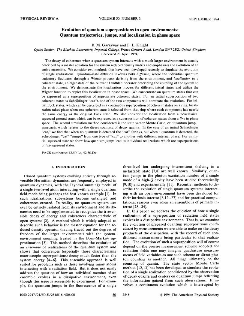
The Fock state, an eigenstate of the harmonic oscilla-tor, is a very nonclassical state and does not remain intactfor very long under the infiuence of dissipation [2]. In aquantum-state diffusion simulation or heterodyne mea-surement, the state localizes and approaches a coherentstate. The process is illustrated in Fig. 5 for the initialstate!n ) with n =9. The initial Wigner function, as de-scribed by W„„in Eq. (30), is shown in Fig. 5(a). Duringa short space of time [Figs. 5(b) and 5(c)], the Wignerfunction loses its circular structure and eventually col-lapses into a single peak located close to the outer rim ofthe initial Wigner function [Fig. 5(d)]. During this pro-cess the mean photon number ( 8 ) simply decays in a

roughly exponential, though stochastic, manner as can beseen in Fig. 6. A decay can also be seen in the meanvalues of the quadratures (X') and ($') in Fig. 7, butonly after nonzero values of these quantities have been es-tablished. The initial state had zero values of (X') and(0') and the development of definite nonzero values isanother manifestation of the localization process. As inthe case of the Schrodinger "cat," localization can beseen in the fluctuations ~ and hF in Fig. 8. These Auc-

tuations reduce to one-half, which is the value for acoherent state. However, the rate of the reduction israther less rapid when compared to the even coherentstate of Fig. 3.

We may suppose that in the localization process the in-itial state may be regarded as divided into coherent statesfrom which one component is selected. In the case of theSchrodinger "cat" we had a choice of two components.In the case of a Fock state there are an infinite number ofcomponents because we can write the Fock state as [51]

(c)

FIG. 5. Localization of a Fock state with n =9. These re-sults are for a single sample undergoing quantum-state diffusion.The Wigner functions are shown for ~t=0, 0.1 0.2, and 1.0 in

(aj-(d).

50 EVOLUTION OF QUANTUM SUPERPOSITIONS IN OPEN ~ ~ ~ 2555

2 0(a)

5-C

4—

1.5—

x

00.0

I

0.5I

1.0I

1.5I

2,0 2.5

0.50.0

I

0.5I

1.0I

1.5I

2.0 2.5

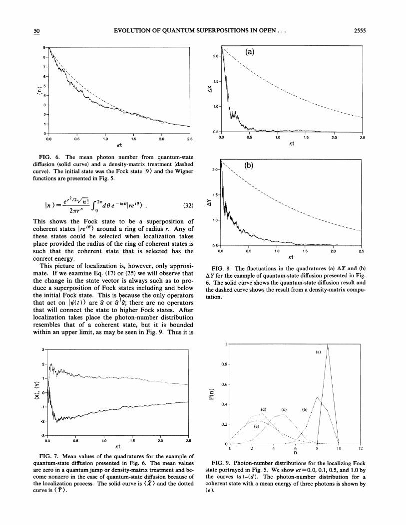
FIG. 6. Thhe mean photon number from quantum-state

curve). The i' '

curve an a densit -ma'

y- atrix treatment (dashede tmual state was the Fock state ~9) an

fun't"n'"' ""nt'din Fi 5~ ~

2/2e(re'e& (32)

1.5-

This shows the Fock state to be a sucoherent states ~!re' )

o e a superposition ofre around a ring of radiu

these states could b 1 cplace provided th d'

e se ected when loccalization takes

such that the he ra ius of the rin o

'g of coherent states is

correct enera e co erent state that isnergy.

is selected has the

Thi's picture of localization is, however, onlt. If i E (17)the change in th

'e q. or (25) we will observe that

a o a coherent state, but it iswithin an upper limit a

u i is boundedimi, as may be seen in Fig. 9. Thus it is

1.0-

0.50.0

I

0.5I

1.0I

1.5I

2.0 2.5

FII . 8. The fluctuations in th

the dashed cq um-state diffusion result and

s e curve shows the result from atation.

rom a ensity-matrix compu-

0.8-

0.6-

0.4—(c) (b)

-30.0

I

0.5I

1.0I

1.5I

2.0 2.5

FIG.G. 7. Mean values of the quadratures~

q o p-s a e i usion presented in Fig. 6. The m

are zero in a quantum'

g. . e mean values

come nonzero in theum jump or densit -matrid

'y- 'x treatment and be-

in t e case of quantum-state diffusth 1 1 t Thpoprocess. The solid curve

'

0.2-

00

III

IIII

II

III

/III/

//

//

I

4 6 8n

I

10 12

FIG. 9. Phhoton-number distributions for thed' F 5 Wig. . We show xt=0.0 0

the curves (a )—(d ). Th. , 0.1, 0.5, and 1.0 by

h 'he photon-number

(e).wi a mean energy of three photons is shown by


necessary for the peak in the photon-number distributionat n to lie at least &n away from the initial photon num-ber of the Fock state (no say) for localization to be comp-leted. A simple calculation shows that for large no weachieve this condition if n -no —+no .Now n gives themean energy at the localization time tl and no gives theinitial energy. Because the decay of the mean photonnumber is roughly exponential (see, for example, Fig. 6) itfollows that n —no exp( atI —), w. hich yields the estimatefor the localization time Irt& —1/+no. Clearly, the timetaken for localizing decreases as the initial photon num-

ber increases.

C. Localization of the squeezed vacuum

0I

0.5I

1.0 1.5

I

I

I

I

I

1

I

I

I

II

The squeezed vacuum may be defined from the actionof the squeeze operator on the vacuum state [52],

~s, 8) =exp[(s/2)[(it ) e' —& e ']I ~0), (33)

FIG. 11. Mean photon number from an initial squeezed vac-uum [Eq. (33)] with s(0)=0.8 as in Fig. 10. The solid curveshows the quantum-jump simulation, the dotted curve showsthe quantum-state diffusion simulation, and the dashed curveshows the result from the density-matrix calculation.

where s is the squeezing factor. Unlike the Fock state,the squeezed vacuum has an orientation in phase space, afeature it shares with the Schrodinger "cat." This axis oforientation is at an angle of 8/2 to the phase-space axesand the Wigner function of the state is a squeezed Gauss-ian function as shown in Fig. 10(a) for s =0.8. Becausethe squeezed vacuum has this orientation we may sup-pose that the localization process will be more definite

0.7

0.6

(a

(a)

0.4—

0.3—

0.0I

0.5I

1.0I

1.5I

2.0 2.5

~ I iJ I ~ I JJsJI

))(~&

. ~k, ~g

0.50.0

I

0.5I

1.0I

2.0 2.5

FIG. 10. Wigner functions in a quantum-state diffusion simu-lation starting from a squeezed vacuum state [Eq. (33)] withs(0)=0.8 and 0=0. In (a) we show the initial state and in (b)we show the Wigner function when at =1.0. In the latter casethe Wigner function has lost much of its squeezing, but is dis-

placed from the phase-space origin.

FIG. 12. Fluctuations in the quadratures during evolutionfrom an initial squeezed vacuum. The parameter and curves aredefined in Fig. 11. Note that under quantum-state diffusion ~and hY are smooth curves, unlike the quantum-state diffusionresult for ( & ) seen in Fig. 11.


than in the case of a Fock state. This is because of theconnection to a heterodyne measurement, an amplitudemeasure, which was outlined in Sec. II C. Indeed, in Fig.10(b} we can see evidence of localization in the displace-ment of the Wigner function from the phase-space origin.As in the case of the Fock states the localization can beregarded as state selection from a group of coherentstates. The squeezed vacuum can be expressed in terms ofGaussian distribution of coherent states along a line inphase space such that [51]

~s, 8) =(2m. sinhs }

X f" dr exp[ r l(—e ' 1)]~r—e' ) . (34)

This means that localization is more likely near thecenter of the distribution.

In Fig. 11 the dotted line shows the decay of the meanphoton number during the decay process. As expected itis stochastic, but loosely follows the density-matrix resultwhich is shown as the dashed line. The surprising resultis found in Fig. 12, where we see that the fluctuations ~and hY follow smooth curves. (Compare this to thequantum-state diffusion simulation of (& ) in Fig. 4.) Inboth cases the fluctuations steadily approach thecoherent state value of one-half. This localization is lessrapid than in the case of the Schrodinger "cat." Notethat to obtain the master-equation result for ~ from thesimulations it is necessary to ensemble average over (2 )and (X' ) separately and then compute ~ from theseaverages.

IV. QUANTUM JUMPSAND THE DECAY OF NONCLASSICAL STATES

~tl~.~%lira &n m~ ci'S

(c)

A. The "jumping cat"

In this section we will consider the quantum jumptheory of an initial Schrodinger "cat" such as the evenand odd coherent states of Sec. III A. The results will becontrasted with quantum-state diffusion. The quantumjump theory naturally divides into two parts: the non-Hermitian evolution and the jumps themselves. We con-sider the non-Hermitian evolution first.

To determine the non-Hermitian evolution with H, ff

[Eq. (4)] we simply have to expand the coherent states inthe Fock basis to find that

atQ 8/2la, +&=I« "",+&,

NQ(r )

where the normalization factor was

(35)

No(t} = '

cosh(~a ~e "'}(even coherent state)

cosh asinh(~a ~e "')

(odd coherent state) .sinh a

(36)

The normalized state (35) represents a Schrodinger "cat"that shrinks in time (see Fig. 3); both of the componentsof the "cat" move towards the phase-space origin while

FIG. 13. A "jumping cat" that was initially comprised of thecoherent states ~a) and

~

—a) with a=2. These results are fora single sample where the internal phase of the cat changes ateach quantum jump. We show the Wigner functions before andafter the first jump (at xt=0.708) in (a) and (b). In (c) and (d)we show the Wigner functions before and after the second jump(at at = 1.127). The same jumps are seen in Figs. 2W.

2558 B. M. GARRA%'AY AND P. L. KNIGHT 50

tanh~a(t)~ (even coherent state)

coth~a(t)~ (odd coherent state),

where for the shrinking "cat"

a(t ) =e "'a(0) .

(37)

(38)

When the Schrodinger "cat"jumps the state vector trans-forms as [Eq. (3)]

~a, +)~~a, + &, (39)

which means that the Schrodinger "cat" jumps from onetype of "cat" to another type of "cat." (See Fig. 13.)During the complete evolution of jumps and non-Hermitian evolution we find that there are essentiallyonly two quantum trajectories: the shrinking evencoherent state and the shrinking odd coherent state. Theeffect of the quantum jumps is simply to switch from oneof these trajectories to the other, or vice versa. This isseen clearly in Fig. 4, which shows by the solid curve themean photon number of the Schrodinger "cat" state as itsevolves and jumps. Similar behavior is seen in Fig. 2 forthe fiuctuation ~ and especially in 5Y because the evencoherent state shows slight squeezing in 6Y whereas theodd coherent state does not.

The principal conclusion in this section is that undercontinuous photodetection a Schrodinger "cat" remains aSchrodinger "cat" as it relaxes to the vacuum state. Thusthe coherence of the two components is maintained bywatching the "cat." Unlike the quantum Zeno effect thiskind of watching does not prevent the decay, it preventsthe decay of the coherence. If we were to consider adifferent type of superposition we may find a different re-sult. For example, if we have a superposition of acoherent state ~p) and the vacuum we would have a typeof Schrodinger "cat" considered in Ref. [10]. However,as soon as there has been a single quantum jurnp wewould only have the single component ~p(t)) left [wherep(t }=exp( at)p(0)]. This r—efiects the gain of informa-tion when a photon leaves the system; as soon as wedetect a photon the possibility of the state ~0) is exclud-ed.

B. Quantum jumps aud Fock states

the coherence of superposition is maintained because it isa pure state. The time-dependent probability (36) indi-cates, as expected, that as t ~ ~ it is impossible for theodd coherent state to avoid at least one jump while thereis a finite probability of 1/cosh

~a

~that the even

coherent state never performs a quantum jump at all.At any time during this shrinking process the probabil-

ity (per unit time) of a quantum jump is given by Eq. (2)as

throughout the evolution. For a Fock state~n ) the prob-

ability of m jumps up to a time t is given by Eq. (16):

nfP (t)=(e"—1) e

m!(n —m )!(40)

C. Quantum jumps aud the squeezed vacuum

!$0(t))= e " S(s,e)~0&,No(t )

where

(41)

S(s, 8) =exp —[(& )' —a e '

] .2

(42)

as in Eq. (33). As before, the normalization Ne( T) is re-

quired because H, ff is non-Hermitian and the state vectorwould otherwise shrink. To proceed we note that

~y (t)) = e is s~ S'(s g)e"'a s~ e "~ s~~~0)No(t )

1 S

No(t ) 2exp —[(8 ) e' e

gZe—ie vi] ~0) (43)

We can rephrase this result by first disentangling theoperators using the SU(1,1) disentangling expressions [54]and then reentangling the result as a new squeezed state.The disentangling results in the state

lf,(t)) =No( t )&coshs

Xexp[e' "'tanhs(Q ) /2]~0),

and when we reentangle we obtain the state as

An account of a related problem has been given byOgawa, Ueda, and Imoto in Ref. [53] where they exam-ined the Husimi function of the density matrix after oneand two photocounts. The initial state in that case was adisplaced squeezed vacuum. Here we will present ananalysis in terms of the pure state evolution that will bevalid for any number of quantum jumps or photocounts.We consider the squeezed vacuum without any displace-ment. We will give details of the integral representationof the time-dependent state in terms of coherent statesand its relation to a Schrodinger "cat" as the number ofjumps increases. However, we first consider the evolu-tion of the state under the effective Harniltonian H, ff andthen we look at the effect of the quantum jumps.

The evolution of ~!g(t })under only the non-HermitianH ff results in the state vector

We consider the case of quantum jumps and Fockstates here only for completeness because their case isvery straightforward. The non-Hermitian evolution (4)has no effect on the state after renormalization, as thejumps (3) cause downwards transitions from Fock state toFock state. The state vector remains nonclassical

where the normalization was found as1/2

coshs(t)No(t)=,

coshs(0)

(45)

(46)


The time-dependent squeezing factor is found to be givenfrom

tanhs(t) =e "'tanhs(0) . (47)

(g(t —~))m/2

& S[s(t),{9]10& .N (t)

(48)

Thus we see that the e8'ect of the non-Hermitian evolu-tion is to decrease the squeezing of the state. The proba-bility of continuous evolution without a quantum jump isgiven by No(t ) .

To obtain the quantum state after m jumps we recallEq. (11) and using Eqs. (41)—(47) the normalized statevector is found as

a-S[s(t), e]lo& .N' (t)(49)

The photon-number distribution and Fock state expan-sion are found from the Fock state expansion of thesqueezed vacuum [55]:

To find the probability of reaching this state we would re-quire the normalization factor N (t), although we will

focus on the state itself rather than the probability offinding it, and so write it in the form

I

S[ ( ) 8]l0&& + tanhs(t }e' (21)!

l21 &N' (t ) N' (t )& coshs(t ) ~=p' (m+n)/2

tanhs(t )e' (m+n )!2 [(m +n )/2]!&n!

ln&. (50)

The photon-number distribution contains only even pho-ton numbers or only odd photon numbers depending onthe number of jumps. We can now formally derive thenormalization N' (t ) from

[N' (t }]'= 1

coshs tm+n

tanhs ( t )e '

m+n even

P(n)= 1

2n sinhs(t}[N' (t)] n!

X x y exp —x +y 2tanhs t

x(xy)

and thus

(54)

[(rn+n )!]I [(m+n )/2]!] n!

(51)[N' (t)]'=

Im 8/2

N' (t)&2m sinhs(t)

X drexp —r e '"—1

xr lre' (52)

This is an infinite sum; later we will find a better expres-sion in the form of a finite sum.

To obtain the integral representation of the new state(49} in terms of coherent states we may extend Eq. (34) sothat [56]

X x y exp —x +y 2tanhs t

+xy](xy) (55)

which can be expressed in polar coordinates. When theradial integral is carried out we obtain

m! sd

(sis8sos8)"2 0 —,

' coths t —sin cos8

(56)

as can be verified from the Fock state expansion. Thusthe distribution of coherent states is the Gaussian of thesqueezed vacuum modified by r . The integral represen-tation (52} leads to a better expression for the normaliza-tion. We obtain first

i(m+n)8(n l@(t) &

=N' {t )v'2m sinhs ( t }n!

X f dr exp[ —r /(2tanhs(t))]r

which can be integrated to give the finite series

[N' (t)] =2m sinhs(t)m!2= tanhs{t)2 1 —tanhs t

11tanhs(t )—1

tanhs( t )+ 1

(2m —21 —1)!!(21—1)!!(m 1)!1!

m

{57)

so that

(53)This series is easier to calculate than the infinite series(51) above. The first few values yields


NO=1,

N', =sinhs(t ),N2 =&3 sinh s(t ),N3 =&3 sinh s (t )+2+3 coth2s (t ) .

We can also use the integral representation (52) to ex-amine the state (49) for large m. By carrying out asaddle-point approximation on the function in the in-

tegrand we obtain

im 0/2

g (+re) J dr exp[ —2(r+ro)2/(e2'" —1))ire' ~2),N' (t)&2n sinhs(t) +

where

ro(t ) =&m [exp[2s(t ) ]—1 ) /2= m tanhs(0)e "'—tanhs(0)

(60)

Is, 8,a) =B(a)S(s,8)IO), (61)

(where 8 represents the displacement operator) has therepresentation in terms of coherent states

I s, 8,a ) = ( 2m. sinhs )

X drexp —r e '—1

+ir Im(ae ' )]Ia+re' ) .

(62)

Now a more general squeezed state, the squeezed and dis-placed vacuum

This is because at each jump the state vector becomes in-creasingly complicated and the approximate state vector(63) comprises two Schrodinger "cat" components with aseparation that depends on the number of jumps m

through Eq. (60). However, there are two families of tra-jectories reflected in the change of sign in Eq. (63) and inthe fact that the state vector contains only even Fockstates for even m and only odd Fock states for odd m. Inthe latter case the mean photon number always ap-

0,2

Ca)

By comparing the approximate representation of thestate for large m with Eq. (62) for the squeezed state wecan see that Eq. (59) approximates a superposition of twosqueezed states located at +roe' in phase space. Thusthe state (49) may be approximated as lo

(63)

with N" ( t ) found frotn the overlap of the squeezed statesas

(64)

(b)

Each of the squeezed state components of thisSchrodinger "cat" has a squeezing of

C).2—

1 +e 2s(t)s'= —' ln2 2(65)

This approximation to the state reveals it to be a specialkind of Schrodinger "cat." Two examples of the exactand approximate photon number distributions are illus-trated in Fig. 14. It is interesting to note that a better ap-proximation is found by using Stirling's formula on Eq.(50), but this does not offer an obvious interpretation.

In Fig. 11 the solid curve shows the quantum jumps ofan initial squeezed vacuum. Unlike the case of theSchrodinger "cat" (the even and odd coherent states) wefind that there are more than two trajectories present.

FIG. 14. The exact (solid line) and approximate (diamonds)photon-number distributions of the state (49) for (a) s =0.8 andm =4 aud (b) s=0.4 and m =7. The results are from Eq. (50)and the Fock state expansion of Eq. (63).


(a)

Q)PI ~

8 I I ~ ~ I gH ba

(c)

FIG. 15. The Wigner functions of the quantum state as it evolves through the first four quantum jumps seen in Figs. 11 and 12.The Wigner functions shown are (a) before and (b) after the quantum jumps at xt =0.079, (c) before and (d) after the quantum jump atxt =0.350, {e)before and (f) after the quantum jump at set =0.574, and (g) before and {h}after the quantum jump at ~t = 1.339


proaches one for large ~t, although for large enough ~tthere is at least one more jump to come. The fluctuationsare shown in Fig. 12 and exhibit a character that is simi-lar to the even and odd coherent states of Fig 2. Howev-er, there is a much greater degree of squeezing in Fig. 12.This can be understood from the approximate solution(63) because the direction of the squeezing of the "cat"components in phase space is at right angles to the direc-tion along which they are aligned. This is more clearlyseen from the plots of the Wigner function shown in Fig.15. The initial Wigner function has been seen in thequantum-state difFusion case in Fig. 10(a) and is clearlysqueezed in the x direction. Figure 15(a) shows the evo-lution under H,~ up to the point of a jump; consequentlythere has only been a reduction in the squeezing accord-ing to Eq. (47). After the first quantum jump in Fig. 15(b)a hole is forming in the center of the Wigner function.Evolution without jumps continues in Fig. 15(c) with afurther loss of squeezing. The second jump in Fig. 15(d)results in a return to squeezing in ~ and a Wigner func-tion that looks remarkably like that of the even coherentstate. This evolves in Fig. 15(e) and jumps in Fig. 15(f),resulting in a Wigner function similar to that of the oddcoherent state. However, we know from Eq. (63) that itis better approximated by the superposition of squeezedstates given there. After a much greater elapse of time[Figs. 15(g) and 15(h)], the Wigner function lacks a closeresemblance to that of a Schrodinger "cat" because sofew photons are left.

extent dictates the size of the fluctuations. Different rep-resentations of the patch in terms of various basis statesresult in different "tilings" of phase space: for an oscilla-tor, energy eigenstates containing specific quanta areessentially annuli with zero mean amplitude, whereascoherent states tile phase space with circles each centeredon a specific mean amplitude. Individual realizations areconditioned by the specific information gained by themeasurement scheme. The two simulation schemes ex-amined here reflect different kinds of conditioning andemphasize their own preferred phase-space tiling as wehave shown. We have illustrated these preferences with anumber of nonclassical superposition states. The locali-zation phenomenon has been exhibited for an initialSchrodinger "cat,"Pock state, and the squeezed vacuum,with the use of the Wigner phase-space quasiprobability.We have presented analytic results for arbitrary initialstates after a finite number of quantum jumps, leading tothe "jumping cat" in the case of an initial superpositionof two coherent states. For the squeezed vacuum wehave shown how the detection of photons results in theemergence of a special Schrodinger "cat" with squeezedstate components.

ACKNOWLEDGMENTS

V. CONCLUSION

A quantum state in phase space is described by a patch(or patches) whose center dictates mean values and whose

This work was supported in part by the United King-dom Science and Engineering Research Council and bythe European Community.

[1) B. W. Shore and P. L. Knight, J. Mod. Opt. 40, 1195(1993),and references therein.

[2] M. Sargent III, M. O. Scully, and W. Lamb, Jr., LaserPhysics (Addison, Wesley, Rading, MA, 1974).

[3] W. H. Louisell, Quantum Statistica/ Properties of acadiation (Wiley, New York, 1973).

[4] J. P. Paz, S. Habib, and W. H. Zurek, Phys. Rev. D 47,488 (1993); W. H. Zurek, Phys. Today 44 (10), 36 (1991);46, 84 (1993); W. H. Zurek, Prog. Theor. Phys. 89, 281(1993); W. H. Zurek, S. Habib, and J. P. Paz, Phys. Rev.Lett. 70, 1187 (1993),and references therein.

[5] E. Joos and H. D. Zeh, Z. Phys. B 59, 223 (1985); D. F.Wa)1s and Cx. J. Milburn, Phys. Rev. A 31, 2403 {1985);S.J. D. Phoenix, ibid. 41, 5132 (1990).

[6] G. J. Milburn, Phys. Rev. A 36, 5271 (1987).[7] Th. Sauter, W. Neuhauser, R. Blatt, and P. E. Toschek,

Phys. Rev. Lett. 57, 1696 (1986); J. C. Bergquist, R. G.Hulet, W. M. Itano, and D. J. Wineland, ibid. 57, 1699(1986); W. Nagourney, J. Sandberg, and H. Dehmelt, ibid.56, 2797 (1986); E. Peik, G. Hollemann, and H. Walther,Phys. Rev. A 49, 402 (1994).

[8] N. Gisin, P. L. Knight, I. C. Percival, R. C. Thompson,and D. C. Wilson, J. Mod. Opt. 40, 1663 (1993).

[9]M. Brune, S. Haroche, J. M. Raimond, L. Davidovich,

and N. Zagury, Phys. Rev. A 45, 5193 (1992).[10]L. Davidovich, A. Maali, M. Brune, J. M. Raimond, and

S. Haroche, Phys. Rev. Lett. 71, 2360 (1993).[11]G. Benson, G. Raithel, and H. Walther, Phys. Rev. Lett.

72, 3506 (1994).[12]H. J. Carmichael, An Open Systems Approach to Quantum

Optics, Lecture Notes in Physics m18 (Springer-Verlag,Berlin, 1993).

[13]J. Dalibard, Y. Castin, and K. Ms(lmer, Phys. Rev. Lett.6S, 580 (1992); K. Mimer, Y. Castin, and J. Dalibard, J.Opt. Soc. Am. B 10, 524 (1993).

[14]Y. Castin, J. Dalibard, and K. Me(lmer, Atomic Physics 13,edited by H. Walther, T. W. Hinsch, and B. Neizert(AIP, New York, 1993),p. 143.

[15]N. Gisin and I. C. Percival, J. Phys. A 25, 5677 (1992); 26,2233 (1993);26, 2245 (1993).

[16]T. P. Spiller, B. M. Garraway, and I. C. Percival, Phys.Lett. A 179, 63 (1993).

[17]H. M. Wiseman and G. J. Milburn, Phys. Rev. A 47, 642

(1993).[18]N. Gisin and Y. Salama, Phys. Lett. A 181, 269 (1993); N.

Gisin, J. Mod. Opt. 40, 2313 (1993).[19]I. C. Percival, J. Phys. A 27, 1003 (1994).[20) G. C. Hegerfeldt and T. S. Wilser, in II International


8'igner Symposium, 1991 (World Scienti5c, Singapore,1992); G. C. Hegerfeldt and M. B.Plenio (unpublished).

[21]C. Cohen-Tannoudji, B. Zambon, and E. Arimondo, J.Opt. Soc. Am. B 10, 2107 (1993).

[22] P. Goetsch and R. Graham, Ann. Phys. (Leipzig) 2, 706(1993).

[23] B. M. Garraway and P. L. Knight, Phys. Rev. A 49, 1266(1994).

[24] B. M. Garraway, P. L. Knight, and J. Steinbach (unpub-

lished).[25] B.M. Garraway and P. L. Knight, in Quantum Optics VI,

edited by J. D. Harvey and D. F. Walls (Springer-Verlag,Berlin, in press).

[26] A. Imamoglu, Phys. Rev. A 48, 770 (1993).[27] W. G. Teich and G. Mahler, Phys. Rev. A 45, 3300 (1992).[28] L. Tian and H. J. Carmichael, Phys. Rev. A 46, 6801

(1992).[29] R. Dum, P. Zoller, and H. Ritsch, Phys. Rev. A 45, 4879

(1992).[30] C. W. Gardiner, A. S. Parkins, and P. Zoller, Phys. Rev.

A 46, 4363 (1992).[31]R. Dum, A. S. Parkins, P. Zoller, and C. W. Gardiner,

Phys. Rev. A 46, 4382 (1992).[32] M. J. Holland, K.-A. Suominen, and K. Burnett, Phys.

Rev. Lett. 72, 2367 {1994);M. J. Holland, D.Phil. thesis,University of Oxford, 1994.

[33]W. K. Lai, K.-A. Suominen, B. M. Garraway, and S.Stenholm, Phys. Rev. A 47, 4779 (1993).

[34] W. K. Lai and S. Stenholm, Opt. Commun. 104, 313(1994).

[35] G. Lindblad, Commun. Math. Phys. 48, 119 (1976).[36] H. M. Wiseman and G. J. Milburn, Phys. Rev. A 47, 1652

(1993);also I. C. Percival (unpublished).

[37] K. Me(lmer (unpublished).

[38] G. J. Milburn, Phys. Rev. A 44, 5401 (1991).[39]H. Moya-Cessa, V. Buick, M. S. Kim, and P. L. Knight,

Phys. Rev. A 48, 3900 (1993).[40] N. Gisin, Phys. Rev. Lett. 52, 1657 (1984); N. Gisin, Helv.

Phys. Acta 62, 363 (1989); L. Diosi, J. Phys. A 21, 2885(1988); Phys. Lett. A 129, 419 (1988); P. Pearle, Phys.Rev. A 39, 2277 (1989); G. C. Chirardi, P. Pearle, and A.

Rimini, ibid. 42, 78 (1990); N. Gisin and I. C. Percival,Phys. Lett. A 167, 315 (1992).

[41] R. Loudon, Quantum Theory of Light, 1st ed .(OxfordUniversity Press, Oxford, 1973).

[42] See, for example, C. W. Gardiner, Quantum Noise

(Springer-Verlag, Berlin, 1991).[43] H. J. Carmichael, S. Singh, R. Vyas, and P. R. Rice, Phys.

Rev. A 39, 1200 (1989}.[44] M. D. Srinivas and E. B. Davies, Opt. Acta 28, 981 (1981);

M. Ueda, Phys. Rev. A 41, 3875 (1990);M. Ueda, N. Imo-

to, and T. Ogawa, ibid. 41, 3891 (1990); M. Ueda and M.Kitagawa, Phys. Rev. Lett. 68, 3424 (1992).

[45] N. Lu, Phys. Rev. A 40, 1707 (1989);S. M. Barnett and P.L. Knight, ibid. 33, 2".".". (1986).

[46] J. Perina, Quantum Statistics of Linear and Nonlinear Op

tidal Phenomena (Reidel, Dordrecht, 1984).[47] U. M. Titulaer and R. J. Glauber, Phys. Rev. 145, 1041

(1966); D. Stoler, Phys. Rev. D 4, 2309 (1971); Z.Bialynicka-Birula, Phys. Rev. 173, 1207 (1968).

[48] K. Vogel and H. Risken, Phys. Rev. A 40, 2847 (1989);D.T. Smithey, M. Beck, M. G. Raymer, and A. Faridani,Phys. Rev. Lett. 70, 1244 (1993).

[49] B. M. Garraway and P. L. Knight, Phys. Rev. A 46, 5346(1992).

[50] V. Buzek, A. Vidiella-Barranco, and P. L Knight, Phys.Rev. A 45, 6570 (1992}.

[51]P. Adam, J. Janszky, and A. V. Vinogradov, Opt. Com-

mun. 80, 155 (1990); see also C. W. Gardiner, Quantum

Noise (Springer-Verlag, Berlin, 1991);V. Buick and P. L.Knight, Opt. Commun. 81, 331 (1991);V. Buick and P. L.Knight, in Progress in Optics, edited by E. Wolf (North-

Holland, Amsterdam, in press).[52] R. Loudon and P. L. Knight, J. Mod. Opt. 34, 709 (1987),

and references therein.

[53]T. Ogawa, M. Ueda, and N. Imoto, Phys. Rev. A 43, 6458(1991).

[54] R. Gilmore, J.Math. Phys. 15, 2090 (1974).[55] H. P. Yuen, Phys. Rev. A 13, 2226 (1976).[56] P. Adam, I. Foldesi, and J. Janszky, Phys. Rev. A 49, 1281

(1994)~

Documents

Evolution of quantum superpositions in open environments: Quantum trajectories, jumps, and localization in phase space