EVLA Memo 110

The Effect of Amplifier Compression by Narrowband RFI

on Radio Interferometer Imaging

Rick Perley and Bob Hayward

April 25, 2007

Abstract

An experiment is described which has permitted direct measurement of the effects from couplingout-of-band emission through the third-order intermodulation product into the astronomical bandof interest, as a function of the degree of compression of a front-end amplifier. The coupling wasmeasured by injecting a 1545 MHz tone into four of the VLA’s FE amplifiers, and measuring thephase and amplitude of the 1665 MHz OH maser at its ‘reflected’ frequency of 1425 MHz, as thesaturating tone power was varied.

We find the following effects:

• The effective gain of the compressed amplifiers for astronomical signals is reduced by abouttwice the compression level.

• The correlation coefficient of in-band emission is reduced by ∼5% at 1 dB compression, andby ∼20% at 3 dB compression, due to the addition of incoherent out-of-band emission.

• Out-of-band emission is reflected into the band of interest at a level of about 1% of its naturalstrength at 1 dB compression, and ∼25% at 3 dB compression.

• The phase of the reflected emission rotates at typically twice the natural fringe rate, relativeto the fringe-stopped emission in the observing band.

The rapid phase rotation of the reflected emission will in general provide considerable attenuationof these signals in interferometric imaging.

1 Introduction

Radio interferometers currently in planning or under construction, particularly those working in themeter and centimeter wavelength bands, are designed with very wide bandwidths – often exceeding 2:1in bandwidth ratio – to maximize continuum sensitivity and to enable unrestricted frequency access forspectral line observations. These wide bandwidths will however permit strong radio-frequency inter-ference (RFI) into the amplification and signal transmission systems, with the likelihood of amplifiercompression and non-linear response. Although good engineering design can provide very high linearity,there will always be some signals entering the system which will cause, at least momentarily, compres-sion in the analog signal system. The consequences of observing with amplifiers operating in theirnon-linear regimes can be serious – power in the fundamental is shifted to higher harmonics, causingan effective loss of gain, and a host of intermodulation products which can shift out-of-band informa-tion into the astronomical band of interest. The latter of these is the most serious for interferometricimaging, and is the subject of this memorandum.

Our first attempt to study the consequences of compression [1] utilized the high temperature broad-band solar calibration noise diodes contained within each antenna. These turned out to be not strong

1

enough to set the system far enough into compression to cause any notable effects. In any event, theuse of broadband signals to saturate the receivers is not a good model for the anticipated operatingenvironment, where strong quasi-CW signals are responsible for the compression.

Our second attempt [2] utilized a strong CW tone to drive the C-band receivers of four VLAantennas to compression levels between 1 and 6 dB. This experiment was successful in determiningthe modest loss of SNR due to compression, and showed that even with these levels of compression,there was no measureable loss of closure – in essence, the astronomical information contained withinthe coherence function was preserved, albeit with lower sensitivity.

Unfortunately, due to the setup chosen for that experiment, the 3rd-order intermodulation productitself was filtered out, and we were unable to measure the amplitude and phase of the reflected signalin the observing band. This filtering, although desirable in the sense of keeping unwanted reflectedinformation out of the band of interest, will not occur in practice, as the entire front-end bandpass willnormally be present at the saturating element in the analog receiver chain.

It is important both for the design of wide-bandwidth radio telescope receivers, and for deciding onmitigating strategies, that the strength of these third-order products, and their ramification on imagingbe understood. In this, our third (and we hope last!) study, we report the results of an experimentspecifically designed to measure the 3rdorder harmonic coupling due to amplifier gain compression.

2 Non-Linear Characteristics of Amplifiers in Compression

In [2] we presented a short mathematical description of how amplifier compression will shift informationfrom one frequency to another by non-linear coupling. We repeat and extend that analysis here.

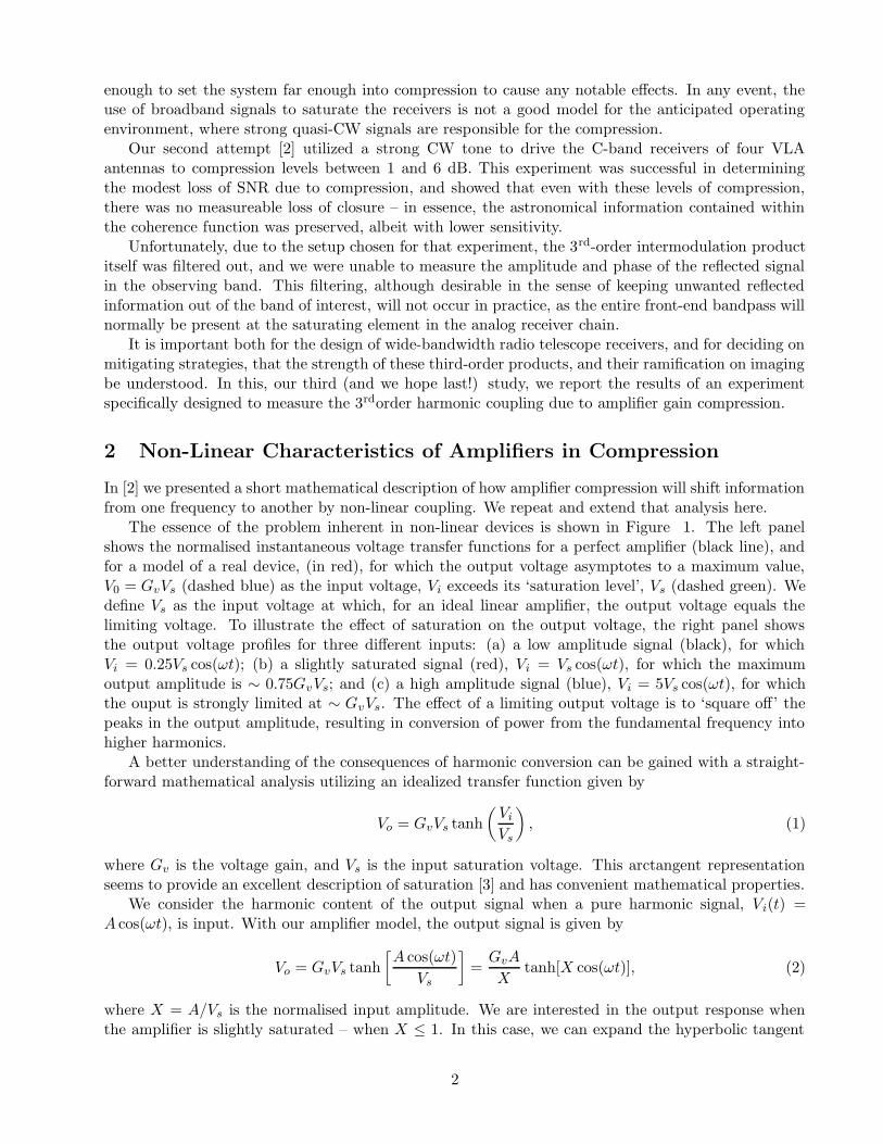
The essence of the problem inherent in non-linear devices is shown in Figure 1. The left panelshows the normalised instantaneous voltage transfer functions for a perfect amplifier (black line), andfor a model of a real device, (in red), for which the output voltage asymptotes to a maximum value,V0 = GvVs (dashed blue) as the input voltage, Vi exceeds its ‘saturation level’, Vs (dashed green). Wedefine Vs as the input voltage at which, for an ideal linear amplifier, the output voltage equals thelimiting voltage. To illustrate the effect of saturation on the output voltage, the right panel showsthe output voltage profiles for three different inputs: (a) a low amplitude signal (black), for whichVi = 0.25Vs cos(ωt); (b) a slightly saturated signal (red), Vi = Vs cos(ωt), for which the maximumoutput amplitude is ∼ 0.75GvVs; and (c) a high amplitude signal (blue), Vi = 5Vs cos(ωt), for whichthe ouput is strongly limited at ∼ GvVs. The effect of a limiting output voltage is to ‘square off’ thepeaks in the output amplitude, resulting in conversion of power from the fundamental frequency intohigher harmonics.

A better understanding of the consequences of harmonic conversion can be gained with a straight-forward mathematical analysis utilizing an idealized transfer function given by

Vo = GvVs tanh

(

Vi

Vs

)

, (1)

where Gv is the voltage gain, and Vs is the input saturation voltage. This arctangent representationseems to provide an excellent description of saturation [3] and has convenient mathematical properties.

We consider the harmonic content of the output signal when a pure harmonic signal, Vi(t) =A cos(ωt), is input. With our amplifier model, the output signal is given by

Vo = GvVs tanh

[

A cos(ωt)

Vs

]

=GvA

Xtanh[X cos(ωt)], (2)

where X = A/Vs is the normalised input amplitude. We are interested in the output response whenthe amplifier is slightly saturated – when X ≤ 1. In this case, we can expand the hyperbolic tangent

2

-2 -1 0 1 2Vi/Vs

-1

-0.5

0

0.5

1

Vo/G

vVs

0 200 400 600 800 1000Time

-1

-0.5

0

0.5

1

Vo/G

vVs

1%

1dB

Figure 1: Left Panel: The black line shows the instantaneous voltage transfer function ofan ideal, linear, amplifier. The red line shows an idealization of a real amplifier, for whichthere exists an asymptotic limiting voltage Vo shown by the dashed blue lines. The greendashed lines define the saturation voltage, Vs, defined by Vo = GvVs. Also shown are the inputamplitudes corresponding to the 1% and 1dB compression levels. Right Panel: Oscillographs ofthree voltage outputs, demonstrating the responses to a non-saturating sinusoidal input (black)Vo = 0.25Vs cos(ωt), slightly saturating input (red), Vi = Vs cos(ωt), and heavily saturatinginput (blue), Vi = 5Vs cos(ωt).

to find, for the normalized output voltage,

V0

GvA= cos(ωt) −

X2

3cos3(ωt) +

2X4

15cos5(ωt) −

17X6

315cos7(ωt) + · · · (3)

The series formally converges for |X| < π/2.We are interested in the power in the various harmonics of the fundamental. These can be de-

termined from expanding the odd powers of the cosine function into its harmonic components1 whichallows us to write the normalized output amplitude as

Vo

GvA= F1 cos(ωt) + F3 cos(3ωt) + F5 cos(5ωt) + · · · (4)

where the amplitude coefficients, Fn, are

F1 = 1 −X2

4+

X4

12−

17X6

576+ · · · (5)

1conveniently done, using the relation, valid for n odd,

cosn(θ) =1

2n−1

(n−1)/2∑

k=0

(

n

k

)

cos(n − 2k)θ

3

F3 = −X2

12+

X4

24−

119X6

1696+ · · · (6)

F5 =X4

120−

17X6

360+ · · · (7)

The power within each component is found from squaring these coefficients. This exercise shows thatthe spectral content of the output voltage is composed entirely of odd harmonics of the fundamentalinput frequency.

The compression C is defined by the ratio of the power in the fundamental harmonic of the outputsignal (GvAF1)

2, divided by that provided by an ideal, linear amplifier of the same low-voltage gain,(GvA)2. Thus, we find

C =

[

1 −X2

4+

X4

12−

17X6

576+ · · ·

]2

(8)

This equation can be solved algebraicly to find that at 1% compression (C = 0.99), A1% = 0.142Vs,and at 1 dB compression, (C = 0.7943), A1dB = 0.708Vs. The input power level at the 1% compressionlevel is 13.9 dB below that of the 1 dB compression level.2.

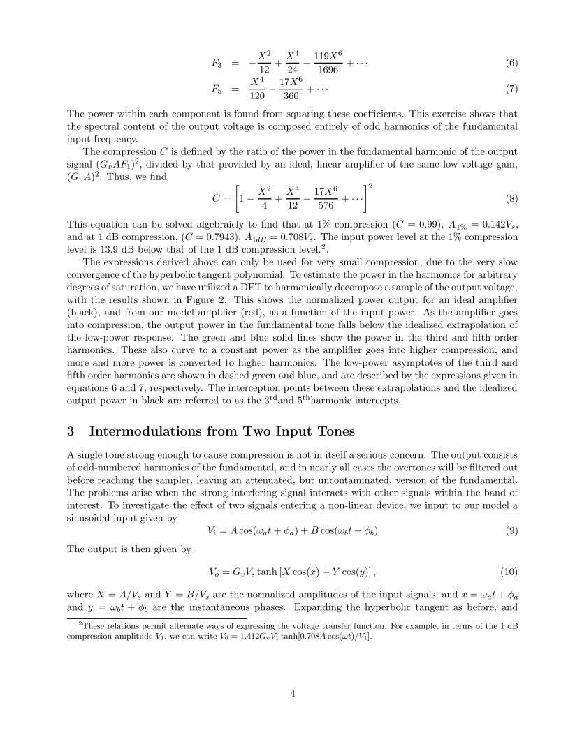
The expressions derived above can only be used for very small compression, due to the very slowconvergence of the hyperbolic tangent polynomial. To estimate the power in the harmonics for arbitrarydegrees of saturation, we have utilized a DFT to harmonically decompose a sample of the output voltage,with the results shown in Figure 2. This shows the normalized power output for an ideal amplifier(black), and from our model amplifier (red), as a function of the input power. As the amplifier goesinto compression, the output power in the fundamental tone falls below the idealized extrapolation ofthe low-power response. The green and blue solid lines show the power in the third and fifth orderharmonics. These also curve to a constant power as the amplifier goes into higher compression, andmore and more power is converted to higher harmonics. The low-power asymptotes of the third andfifth order harmonics are shown in dashed green and blue, and are described by the expressions given inequations 6 and 7, respectively. The interception points between these extrapolations and the idealizedoutput power in black are referred to as the 3rdand 5thharmonic intercepts.

3 Intermodulations from Two Input Tones

A single tone strong enough to cause compression is not in itself a serious concern. The output consistsof odd-numbered harmonics of the fundamental, and in nearly all cases the overtones will be filtered outbefore reaching the sampler, leaving an attenuated, but uncontaminated, version of the fundamental.The problems arise when the strong interfering signal interacts with other signals within the band ofinterest. To investigate the effect of two signals entering a non-linear device, we input to our model asinusoidal input given by

Vi = A cos(ωat + φa) + B cos(ωbt + φb) (9)

The output is then given by

Vo = GvVs tanh [X cos(x) + Y cos(y)] , (10)

where X = A/Vs and Y = B/Vs are the normalized amplitudes of the input signals, and x = ωat + φa

and y = ωbt + φb are the instantaneous phases. Expanding the hyperbolic tangent as before, and

2These relations permit alternate ways of expressing the voltage transfer function. For example, in terms of the 1 dBcompression amplitude V1, we can write V0 = 1.412GvV1 tanh[0.708A cos(ωt)/V1].

4

-5 0 5 1010*Log(Pi/Ps)

-80

-60

-40

-20

0

10*L

og(P

o/GP s)

LinearFundamental3rd OrderFifth Order

1 dB

3 dB

6 dB

Figure 2: The power in the fundamental, 3rd-order, and 5th-order harmonics for our idealizedamplifier response. Marked are the 1, 3, and 6 dB compression points, where the output powerin the fundamental harmonic is reduced by a factor of 0.795, .501, and .251, respectively fromthat of a purely linear device. The 1% compression point is located -13.9 dB below the 1 dBpoint. The intercepts between the low-power extrapolations shown in dashes and the linearresponse in black are the 3rdand 5thorder intercepts.

harmonically decomposing to the third order only, we find

V0

Gv= A

(

1 −X2

4−

Y 2

2

)

cos x + B

(

1 −Y 2

4−

X2

2

)

cos y − A

(

X2

12

)

cos(3x) − B

(

Y 2

12

)

cos(3y)

−A

(

XY

4

)

[cos(2x − y) + cos(2x + y)] − B

(

XY

4

)

[cos(2y − x) + cos(2y + x)] (11)

In addition to the two fundamental and two third-order harmonics, we see the presence of fourintermodulation products – terms at frequencies given by ω = 2ωa − ωb, 2ωb − ωa, 2ωa + ωb, and2ωb + ωa. The two difference terms are of special concern, as they will normally lie close to the twoinput signal frequencies, and hence can lie within the system passband. The other two (summed)intermodulation products can normally be ignored as they will lie outside the bandwidth of the systemresponse.

Extending the analysis to include 5thorder products adds the two fith-order harmonics, and eightnew intermodulation products to the output spectrum. As an amplifier goes deeper into compression,every pair of input signals will produce tens or even hundreds of intermodulation products, many ofwhich will appear within the desired bandpass.

In general, we note that the strength of the third-order intermodulation products rises as A2B,or B2A, whereas the power in the fundamentals rises slower than with A or B. Thus, the ratio ofthe power in the intermodulation products to that of the fundamental signals rapidly increases withincreasing amplifier compression.

5

We now consider the case where the ‘Y’ input signal, representing the RFI, is strong enough tocause gain compression, and the ‘X’ signal, representing the astronomical information, is very weak.Thus, we assume Y � X, (so that B � A), that X � 1, and that Y ≤ 1. Dropping terms much lessthan one, we can then write the output signal, normalized to the idealized output amplitude of A, as

V0

GvA=

(

1 −Y 2

2

)

cos x+R

(

1 −Y 2

4

)

cos y−R

(

Y 2

12

)

cos(3y)−R

(

XY

4

)

[cos(2y − x) + cos(2y + x)]

(12)where R = B/A is the amplitude ratio between the interference signal and the astronomical signal.This formulation allows us to compare the strength of the output harmonics to that of the desired(fundamental) output. Because of the approximations involved, the terms shown are the low-powerapproximations of the actual relations. These expressions should not be employed for compressionlevels exceeding 1 dB.

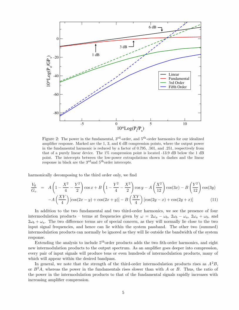
To obtain the amplitudes of all output spectral components over a wide range of input RFI powers,we have employed a DFT routine to harmonically decompose the signal described in Eqn. 10. Theresults are shown in Figure 3. In this simulation, there were two tones submitted to the model amplifier.

-20 -15 -10 -5 0 5 1010*Log(PRFI/Ps)

-100

-50

0

50

10*L

og(P

o/GP s)

RFI Fundamental

Signal Fundamental

RFI 3rd Harmonic2*RFI - Signal Fundamental

2*Signal Fundamental - RFI

Signal 3rd Harmonic

Figure 3: Showing all the fundamental, 3rd-order harmonics, and 3rd-order intermodulationproducts for our amplifier model, as a function of the power in the saturating RFI signal. Theastronomical signal strength is fixed 40 dB below the saturation power. The blue line showsthat the power in the fundamental of the saturating tone asymptotes to a constant value as theamplifier goes into compression. The red line shows the power in the (constant) astronomicalsignal, which declines as its power is shifted into higher harmonics. The purple line shows the riseof the third-order intermodulation product, whose power approaches that of the astronomicalsignal fundamental as saturation increases.

The ‘signal tone’ was fixed at a power level 40 dB below the saturation power, to ensure that it is notresponsible for the amplifier compression, while the ‘RFI tone’ was varied from -40 dB below to +60dB above the saturation power. The power in the various harmonics and intermodulation producrts

6

are shown plotted as a function of the input RFI tone power. As the RFI tone power increases, andthe amplifier goes into compression, the following occur:

• The output power in the RFI signal (blue) rises close to linearly, then asymptotes to a constantlevel as the amplifier goes into compression. The ratio between the extrapolation and outputpower defines the level of compression.

• The output power of the (constant input) astronomical signal (red) slowly declines, as the com-pression limits the range of its voltage, and converts fundamental harmonic power into overtonesand intermodulation products. Notable is that the loss in signal power is twice that of the RFIpower for low levels of compression.

• The power in the 3rdharmonic of the RFI (green) rises quickly, following the same relation shown inFig. 2. As this tone will normally be filtered out before reaching subsequent stages of amplificationor sampling, it is of no concern.

• The 3rdharmonic of the signal power (magenta) is very weak, and of no concern.

• The intermodulation products formed from twice the signal frequency and the RFI frequency(2ωsig ± ωRFI) (brown) are also very weak, and of no consequence.

• The two intermodulation products formed from twice the RFI frequency and the signal frequency(purple) (ω

−= 2ωRFI −ωsig, and ω+ = 2ωRFI +ωsig) rise quadratically, and approach the power

of the astronomical signal itself as the amplifier goes into compression. The summed responsewill normally lie outside the passband, so is of no concern. The difference frequency will normallylie in the desired bandpass, and is the signal of concern.

For modest levels of compression, the fractional loss in signal power scales as 1− (1−Y 2/2)2 ∼ Y 2,while the fractional loss in RFI (tone) power scales as 1 − (1 − Y 2/4)2 ∼ Y 2/2. thus, the fractionalloss in astronomical noise is twice that in tone power. Similarly, the signal attenuation, expressed indecibels, is twice that of the tone attenuation 3.

Hence, when the amplifier is at a 1% compression due to the RFI, the signal output is reduced by2%, and when the compression is 1dB, the astronomical signal is reduced by ∼ 2dB. This behaviorcan be understood by noting that the weak astronomy signal voltage is added to that of the saturatingRFI, and because of the non-linear nature of the transfer function, suffers a greater compression thanthat of the RFI. In the limit, when the RFI amplitude is so great that the output is a pure switchingsquare wave, the power in the astronomy signal will be entirely lost, while that of the RFI is limitedto that offered by the fundamental harmonic component of the output saturation level.

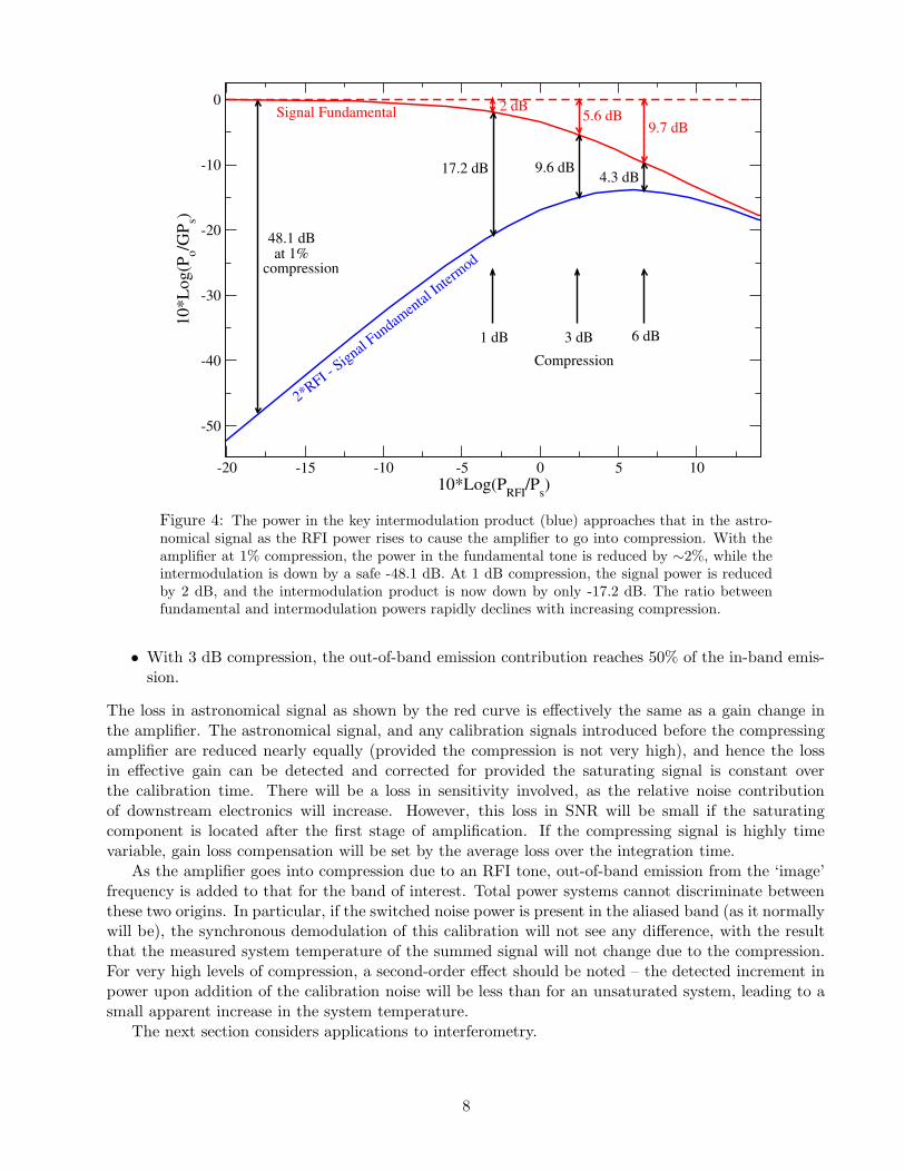
The relation between the astronomical signal power and the key intermodulation product is shownin detail in Figure 4.

Three important conclusions arise from this:

• Amplifier compression causes a significant reduction in astronomical signal power. The loss isby a negligible 2% at 1% compression, but reaches a significant 2 dB (27%) when the amplifierhas reached a 1 dB compression. In some circumstances, this loss can be corrected, as discussedbelow.

• The coupling of the intermodulation product signal into the astronomical band is negligible at1% compression levels, but becomes significant (2%) at 1 dB compression. Thus, at this level ofcompression, a strong out-of-band spectral line can appear in the band of interest, diminished bya factor of ∼ 50.

3If this is not immediately obvious, recall that ln(1 + x) = x − x2/2 + x3/3 − · · ·

7

-20 -15 -10 -5 0 5 1010*Log(PRFI/Ps)

-50

-40

-30

-20

-10

0

10*L

og(P

o/GP s)

48.1 dBat 1%

17.2 dB

2 dB

9.6 dB

9.7 dB

4.3 dB

5.6 dBSignal Fundamental

compression

2*RFI - Signal F

undamental

Intermod

1 dB 3 dB 6 dBCompression

Figure 4: The power in the key intermodulation product (blue) approaches that in the astro-nomical signal as the RFI power rises to cause the amplifier to go into compression. With theamplifier at 1% compression, the power in the fundamental tone is reduced by ∼2%, while theintermodulation is down by a safe -48.1 dB. At 1 dB compression, the signal power is reducedby 2 dB, and the intermodulation product is now down by only -17.2 dB. The ratio betweenfundamental and intermodulation powers rapidly declines with increasing compression.

• With 3 dB compression, the out-of-band emission contribution reaches 50% of the in-band emis-sion.

The loss in astronomical signal as shown by the red curve is effectively the same as a gain change inthe amplifier. The astronomical signal, and any calibration signals introduced before the compressingamplifier are reduced nearly equally (provided the compression is not very high), and hence the lossin effective gain can be detected and corrected for provided the saturating signal is constant overthe calibration time. There will be a loss in sensitivity involved, as the relative noise contributionof downstream electronics will increase. However, this loss in SNR will be small if the saturatingcomponent is located after the first stage of amplification. If the compressing signal is highly timevariable, gain loss compensation will be set by the average loss over the integration time.

As the amplifier goes into compression due to an RFI tone, out-of-band emission from the ‘image’frequency is added to that for the band of interest. Total power systems cannot discriminate betweenthese two origins. In particular, if the switched noise power is present in the aliased band (as it normallywill be), the synchronous demodulation of this calibration will not see any difference, with the resultthat the measured system temperature of the summed signal will not change due to the compression.For very high levels of compression, a second-order effect should be noted – the detected increment inpower upon addition of the calibration noise will be less than for an unsaturated system, leading to asmall apparent increase in the system temperature.

The next section considers applications to interferometry.

8

4 Interferometer Response

The preceding analysis considered only the amplitude and power responses due to amplifier compres-sion. In interferometry, the relative phases of the signals are important, and we consider these effectsin this section.

We consider the outputs of two antennas, both of which receive an astronomical signal of frequencyωo. We take one of these antennas as the phase reference. Constant electronic phase shifts are ignoredhere, as it is the time dependency of the differential phase that we are interested in. Antenna 1’s outputis proportional to cos(ωot). The second antenna’s output is proportional to cos[ωo(t− τg)], where τg isthe geometric delay. Each signal then passes through an amplifier which has been put into compressionby a signal of frequency ωr. The third-order intermodulation signal for the first antenna has a timedependance of cos[(2ωr−ωo)t], while for the second antenna, it is given by cos[(2ωr−ωo)t−ωoτg +2φr],where φr is the phase of the RFI saturating signal at antenna 2, relative to that of antenna 1.

In order to maintain coherence, the signal of antenna 1 must be delayed by a time equal to thegeometric delay applicable to antenna 2. Hence, the time dependency of the signal on antenna onefollowing the insertion of the delay is: cos[(2ωr − ωo)(t − τg)]. The output from the correlator is givenby the low frequency component of the product of the signals – the phase difference – from antennasone and two: cos(2ωrτg +2φr). The phase rate of the product is the observable of interest, and is givenby

φ̇ = 2ωrτ̇g + 2φ̇r (13)

where τ̇g = −ωeBu cos δ/c is the rate of change of delay, ωe = 7.27×10−5 rad/sec is the angular rotationrate of the earth, and Bu/c is the light-travel time of the E-W component of the baseline. This resultis independent of whether the interferometer is ‘direct’, or employs a local oscillator conversion, withappropriate phase rotation.

The second term in the RHS of Eqn. 13 accounts for a phase differential in the saturating signalbetween stations. For stationary RFI, this term will be close to zero (non-zero being possible due tochange in refraction, or antenna motion). For the experiment to be described in the next section, thesaturating signal had a phase difference due to its origin.

We now consider the effect of the aliased signal on the correlation coefficient. The correlator doesnot measure the visibility amplitude directly, but rather estimates the correlation coefficient. This isconverted to a visibility flux density by a correction factor dependent upon the system temperaturesof the two antennas involved. We have argued above that the broadband noise aliased into the bandof interest due to a strong RFI tone retains the switched noise used for estimation of the systemtemperature, so that no significant change in system temperature will be measured due to the amplifiercompression. This is not the case for the correlation coefficient, as the aliased noise does not retain eitherthe correct phase, nor the phase rate, of the emission in the band of interest. Hence, the measuredcorrelation coefficient will be reduced by a factor dependent upon the coupling of the out-of-bandemission into the band of interest. The measured correlation coefficient will be reduced as

ρ =ρ0

1 + ε(14)

where ρ0 is the correlation coefficient for the band of interest, and ε is the fractional contribution ofthe aliased signal to the fundamental signal. We can use the relations shown in Figure 4 to estimatethe loss in correlation coefficient, and hence, presuming the system temperature is not affected, theapparent loss in correlated flux density. These are shown in Table 1.

5 Experiment Setup

The primary goal of this experiment was to measure the coupling of the 3rd-order intermodulationresponse through observations of an astronomical source when the L-Band receivers on four VLA

9

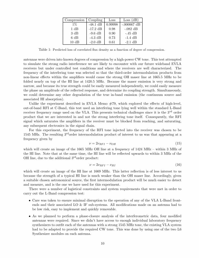
Compression Coupling Loss Loss (dB)

1% -48.1 dB 0.99998 -.000067 dB1 dB -17.2 dB 0.98 -.082 dB3 dB -9.6 dB 0.90 -.45 dB6 dB -4.3 dB 0.73 -1.4 dB10 dB -2.0 dB 0.61 -2.1 dB

Table 1: Predicted loss of correlated flux density as a function of degree of compression.

antennas were driven into known degrees of compression by a high-power CW tone. This test attemptedto simulate the strong radio interference we are likely to encounter with our future wideband EVLAreceivers but under controlled test conditions and where the receivers are well characterized. Thefrequency of the interfering tone was selected so that the third-order intermodulation products fromnon-linear effects within the amplifiers would cause the strong OH maser line at 1665.5 MHz to befolded nearly on top of the HI line at 1420.5 MHz. Because the maser emission is very strong andnarrow, and because its true strength could be easily measured independently, we could easily measurethe phase an amplitude of the reflected response, and determine its coupling strength. Simultaneously,we could determine any other degradation of the true in-band emission (the continuum source andassociated HI absorption).

Unlike the experiment described in EVLA Memo #79, which explored the effects of high-level,out-of-band RFI at C-Band, this test used an interfering tone lying well within the standard L-Bandreceiver frequency range used on the VLA. This presents technical challenges since it is the 3rd orderproduct that we are interested in and not the strong interfering tone itself. Consequently, the RFIsignal which saturates the amplifiers in the receiver must be blocked from reaching, and saturating,any subsequent electronics in the signal chain.

For this experiment, the frequency of the RFI tone injected into the receiver was chosen to be1545 MHz. The resulting 3rdorder intermodulation product of interest to us was that appearing at afrequency given by

ν = 2νRFI − νOH (15)

which will create an image of the 1665 MHz OH line at a frequency of 1424 MHz – within 3 MHz ofthe HI line. Note that at the same time, the HI line will be reflected upwards to within 3 MHz of theOH line, due to the additional 3rdorder product:

ν = 2νRFI − νHI (16)

which will create an image of the HI line at 1669 MHz. This latter reflection is of less interest to usbecause the strength of a typical HI line is much weaker than the OH maser line. Accordingly, givena suitable chosen astronomical source, the first intermodulation product will be much easier to detectand measure, and is the one we have used for this experiment.

There were a number of logistical constraints and system requirements that were met in order tocarry out the L-Band compression test:

• Care was taken to ensure minimal disruption to the operation of any of the VLA L-Band front-ends and their associated LO & IF sub-systems. All modifications made on an antenna had tobe low risk, easy to implement and quickly removable.

• As we planned to perform a phase-closure analysis of the interferometric data, four modifiedantennas were required. Since we didn’t have access to enough individual laboratory frequencysynthesizers to outfit each of the antennas with a strong 1545 MHz tone, the existing VLA systemhad to be adapted to provide the required CW tone. This was done by using one of the two L6Synthesizer modules on each antenna.

10

30dB

1300-1800MHz

TCalNoiseDiode

Pol

LNA

HittiteHMC364Divider

RCP

LCP

17dB

Room Temp RF Box

RF Splitter

F4

F4

F4

F4

A

B

C

D

IF-A(RCP)

IF-B(RCP)

IF-C(LCP)

IF-D(LCP)

L6 #1Synthesizer (2-4 GHz)

L6 #2Synthesizer (2-4 GHz)

30dBLNA

17dB

Level SetPad

(14 to 18 dB)

Tone SelectFilter

1550/100 MHz

1425/50MHz

L-Band Dewar

Existing Cpts

Added Cpts

Dewar

Modules

Disabled Path

New Path

Key:

Test Cpts

4 x F4FrequencyConverterModules

SCalNoiseDiode

-30dB

-30dB

-10dB

-10dB

PCal

Input

3200 MHz

Up-Converter

F2

F6F9Post-Amp

41dB

41dB

÷2

NardaAttenuator

0-99 dB

-10dB

1425/50MHz

Power Sensor

1550/100MHz

Attenuator0-99 dB

CW Tone L6#2 Out ÷2 Out PCal In“OFF” 4010 2005 x“ON” 3090 1545 1545

1545

InjectedRFI Tone

RCP

LCP

MHz

1550/100MHz

Power Sensor

Attenuator0-99 dB

Tone P(Out)

Noise Floor

Tone P(In)

Power Sensor

Noise Floor

Tone P(Out)

RCP

LCP

Figure 5: A block diagram showing the modifications to the VLA/VLBA L-band receiversutilized for this experiment. Block components are color coded to show the modifications made.The artificial tone was generated by one of the two L6 synthesizers, divided by two, and insertedinto the signal path through the calibration couplers. Band limiting filters (in gold) were addedto permit turning off the saturating tone by retuning the L6 synthesizer, and to prevent tonepower from saturating subsequent stages of the electronics, as described in the text.

• To permit ‘on-sky’ comparisons, remote control of the CW tone was required in order to enableand disable the saturating signal. This was done using the VLA ‘Observe’ file to control theL6 synthesizer frequency settings so that a judiciously chosen filter would select or reject theinterfering tone.

• To measure the coupling efficiency of the intermodulation product as a function of the degree ofcompression, the experiment was performed with three different levels of amplifier compression– nominally near 1 dB, 3 dB, and 6 dB, on both polarizations of the four modified antennas.

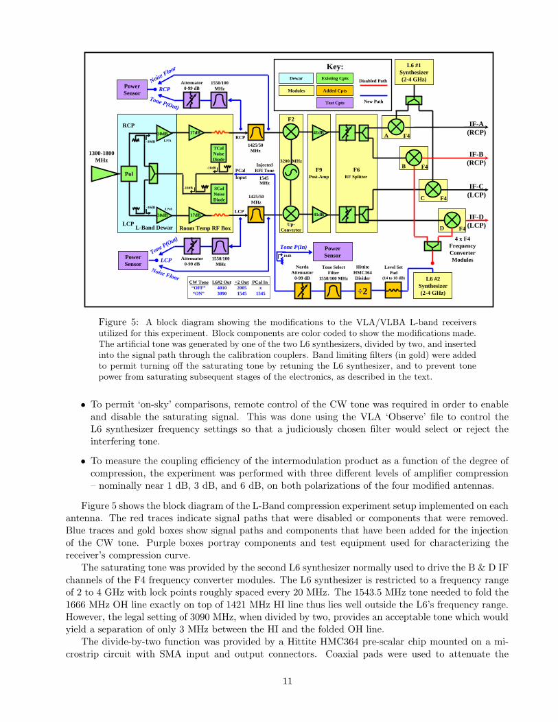
Figure 5 shows the block diagram of the L-Band compression experiment setup implemented on eachantenna. The red traces indicate signal paths that were disabled or components that were removed.Blue traces and gold boxes show signal paths and components that have been added for the injectionof the CW tone. Purple boxes portray components and test equipment used for characterizing thereceiver’s compression curve.

The saturating tone was provided by the second L6 synthesizer normally used to drive the B & D IFchannels of the F4 frequency converter modules. The L6 synthesizer is restricted to a frequency rangeof 2 to 4 GHz with lock points roughly spaced every 20 MHz. The 1543.5 MHz tone needed to fold the1666 MHz OH line exactly on top of 1421 MHz HI line thus lies well outside the L6’s frequency range.However, the legal setting of 3090 MHz, when divided by two, provides an acceptable tone which wouldyield a separation of only 3 MHz between the HI and the folded OH line.

The divide-by-two function was provided by a Hittite HMC364 pre-scalar chip mounted on a mi-crostrip circuit with SMA input and output connectors. Coaxial pads were used to attenuate the

11

1400 1500 1600 1700 1800 19001300

Freq(MHz)

CW Tone“ OFF”

(2005 MHz)

1200

CW Tone“ ON”

(1545 MHz)

Tone SelectFilter

1550/100 MHz

Tone RejectFilter

1425/50 MHz

L-Band RxBroadband

Response

VLA Standard L-Band1300-1800 MHz

Gain Compression inDesired Band due

to Saturating CW Tone

2000

RelativePower

Under L6Control

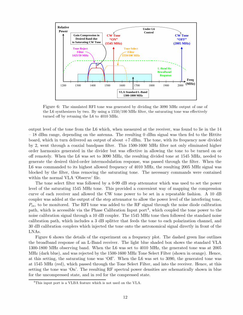
Figure 6: The simulated RFI tone was generated by dividing the 3090 MHz output of one ofthe L6 synthesizers by two. By using a 1550/100 MHz filter, the saturating tone was effectivelyturned off by retuning the L6 to 4010 MHz.

output level of the tone from the L6 which, when measured at the receiver, was found to lie in the 14– 18 dBm range, depending on the antenna. The resulting 0 dBm signal was then fed to the Hittiteboard, which in turn delivered an output of about +7 dBm. The tone, with its frequency now dividedby 2, went through a coaxial bandpass filter. This 1500-1600 MHz filter not only eliminated higherorder harmonics generated in the divider but was effective in allowing the tone to be turned on oroff remotely. When the L6 was set to 3090 MHz, the resulting divided tone at 1545 MHz, needed togenerate the desired third-order intermodulation response, was passed through the filter. When theL6 was commanded to its highest allowed frequency of 4010 MHz, the resulting 2005 MHz signal wasblocked by the filter, thus removing the saturating tone. The necessary commands were containedwithin the normal VLA ‘Observe’ file.

The tone select filter was followed by a 0-99 dB step attenuator which was used to set the powerlevel of the saturating 1545 MHz tone. This provided a convenient way of mapping the compressioncurve of each receiver and allowed the CW tone power to be set in a repeatable fashion. A 10 dBcoupler was added at the output of the step attenuator to allow the power level of the interfering tone,Pin, to be monitored. The RFI tone was added to the RF signal through the noise diode calibrationpath, which is accessible via the Phase Calibration Input port4, which coupled the tone power to thenoise calibration signal through a 10 dB coupler. The 1545 MHz tone then followed the standard noisecalibration path, which includes a 3 dB splitter that feeds the tone to each polarization channel, and30 dB calibration couplers which injected the tone onto the astronomical signal directly in front of theLNAs.

Figure 6 shows the details of the experiment on a frequency plot. The dashed green line outlinesthe broadband response of an L-Band receiver. The light blue shaded box shows the standard VLA1300-1800 MHz observing band. When the L6 was set to 4010 MHz, the generated tone was at 2005MHz (dark blue), and was rejected by the 1500-1600 MHz Tone Select Filter (shown in orange). Hence,at this setting, the saturating tone was ‘Off’. When the L6 was set to 3090, the generated tone wasat 1545 MHz (red), which passed through the Tone Select Filter, and into the receiver. Hence, at thissetting the tone was ‘On’. The resulting RF spectral power densities are schematically shown in bluefor the uncompressed state, and in red for the compressed state.

4This input port is a VLBA feature which is not used on the VLA.

12

To ensure that only the FE was put into compression, and to prevent the powerful 1545 MHz tonefrom saturating downstream electronics, the tone power was prevented from propagating beyond thereceiver by inserting a 1400-1450 MHz bandpass filters at the output of the receiver. This stripped awaythe 1545 MHz RFI tone but preserved the desired astronomical signal around the HI line frequency.

When considering the effects of compression in an amplifier, it is generally expected that the outputpower of the unit integrated over its total frequency range will remain constant. When a strong CWsignal is fed into an amplifier, it will generate many harmonics and intermodulation products. Asthe input level is increased, more and higher level harmonics are generated (at least until the harmfuldamage point is reached) which will effectively reduce the gain seen at the fundamental frequency ofthe tone, as shown in Figures 3 and 4. This reduction is how the 1 dB compression point of an amplifieris both defined and determined. For low-level signals, the Pout/Pin ratio is, by definition, the gain ofthe amplifier. As the amplifier begins to saturate, an increase in the input level will no longer producea proportional increase of the output signal. When the apparent gain drops by 1 dB, the measuredoutput power level is thus defined as the amplifier’s 1 dB compression specification (often denoted asthe P1dB point). The single-ended cryogenic low-noise amplifiers which we use in VLA L-Band receiverstypically have a P1dB of 0 dBm. Thus if the amplifier has a gain of 35 dB, when the input level is -34dBm, its output will be at 0 dBm. That is, the amp will exhibit an effective gain of 34 dB when it isoperated at its 1 dB compression point.

As will be discussed in detail later, the L-Band receivers were driven to their 1 dB compressionpoint when the CW tone was typically at -15 dBm. It turned out that it was not the LNAs that aresaturating in this experiment, but the first stage of post-amps following the LNAs. A back-of-the-envelope calculation of the power levels being experienced by the amplifiers in the signal path whenthe receiver is at its 1dB compression point is given in Table 2

L-Band Receiver Signal Path Location Loss or Gain Power Level(dB) (dBm)

Tone Power measured by Power Meter (Pin) – -15Input of Meter Coupler +10 -5Output of Pcal Coupler -10 -15Output of Cal Splitter -3 -18Output of Cal Coupler -30 -48Output Level of LNA (P1dB ∼ 0dBm) +35 -13Output Level of Post-Amp (P1dB ∼ −5 dBm) +17 -4

Table 2: Estimates of typical power levels occuring in the L-Band compression test.

At the 1dB compression point, the input power at the LNAs was around -48 dBm while the resultingoutput was about -13 dBm, which is more than 10 dB below the 1 dB compression point of 0 dBm forthe low noise amplifier. The post-amp output, however, has a measured P1dB of -5 dBm. When theoutput is at -4 dBm, the post-amp will be at its 1 dB compression point.

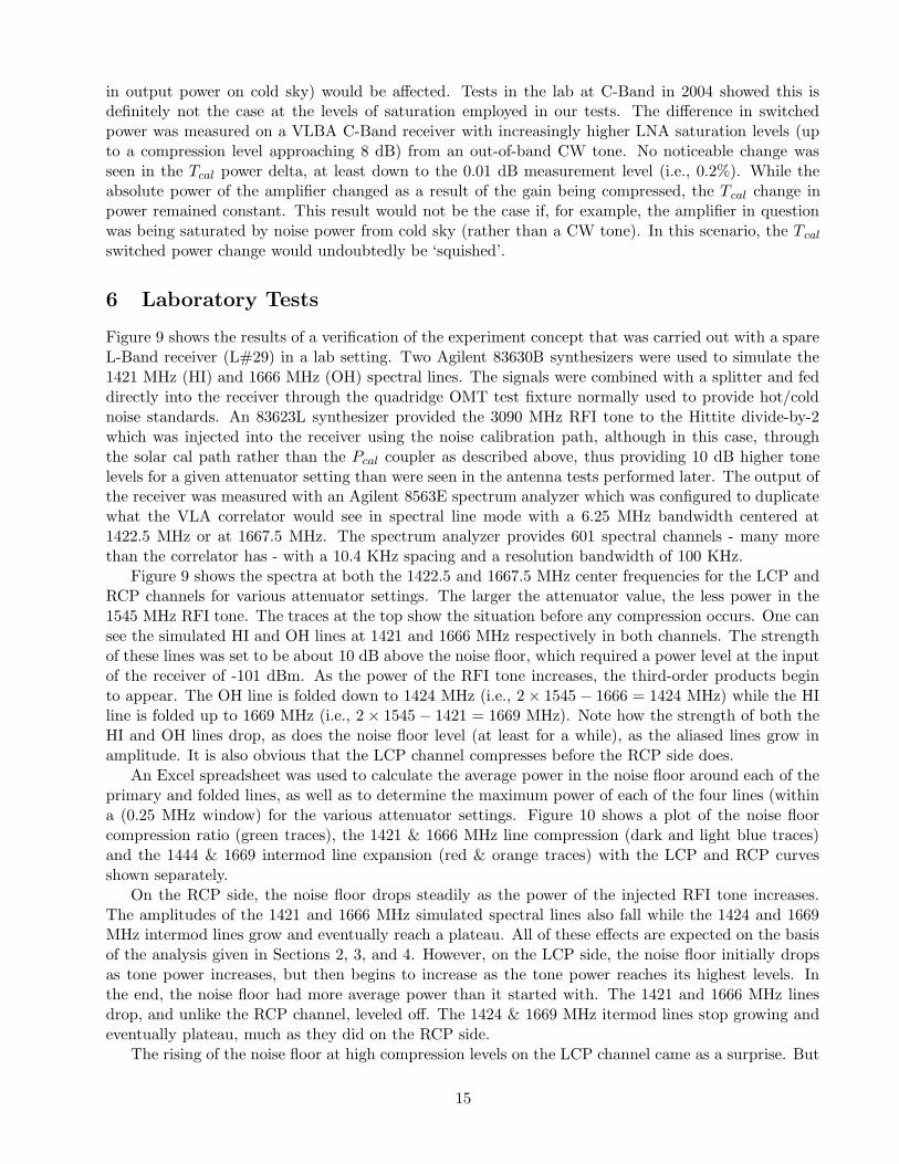
A picture of the setup used in the lab is shown in Figure 7. This shows the Hittite divide-by-2board along with the use of the Pcal input port. Figure 8 shows the actual test setup as implementedon Antenna 23. Of note is the step attenuator along with the 1500-1600 MHz filter and 10 dB testcoupler. The C-clamp that is used to mount the test tone components may seem rather jury-riggedbut in fact provides a simple yet functional way to execute the required modifications.

One advantage of using the Pcal path for injecting the 1545 MHz RFI tone was that the Tcal featurewas preserved. Unlike the earlier C-Band compression test described in EVLA Memo #79, this meantthat the switched noise power signal remained available for calibrating each L-Band system during theexperiment. One might assume that in a saturated receiver, the change in power between the Cal Offand Cal On (typically set to about 10% of Tsys, which corresponds to several tenths of a dB increase

13

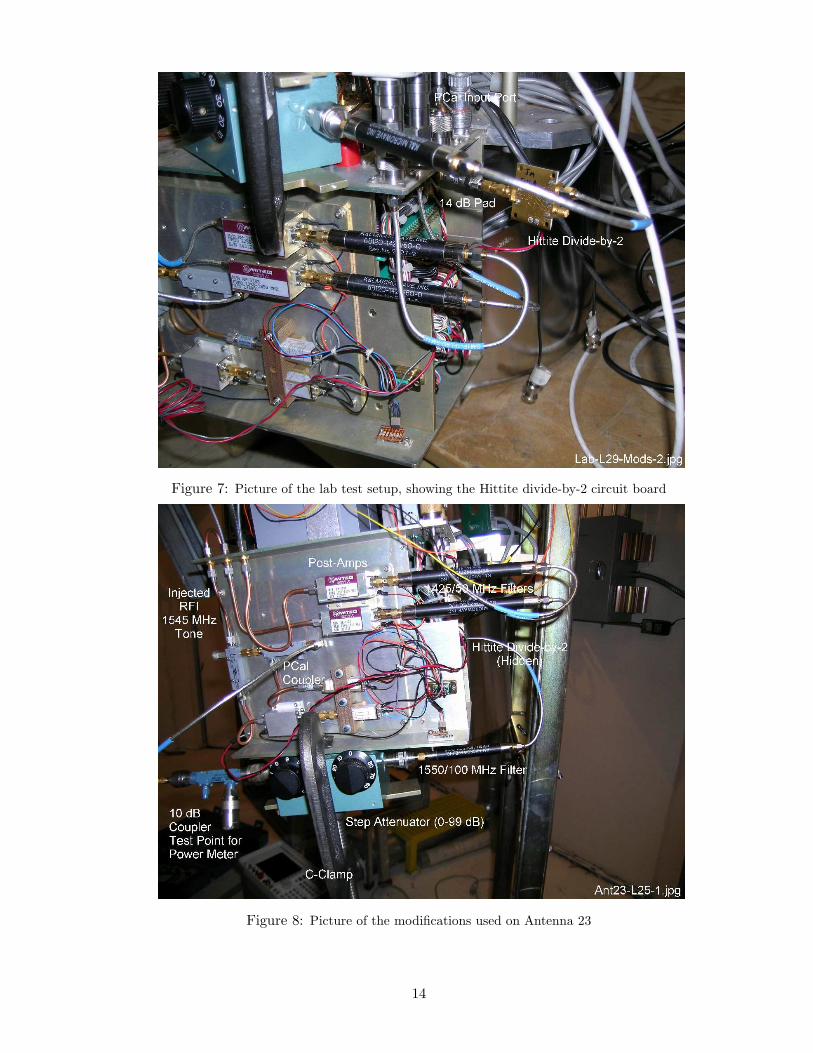
Figure 7: Picture of the lab test setup, showing the Hittite divide-by-2 circuit board

Figure 8: Picture of the modifications used on Antenna 23

14

in output power on cold sky) would be affected. Tests in the lab at C-Band in 2004 showed this isdefinitely not the case at the levels of saturation employed in our tests. The difference in switchedpower was measured on a VLBA C-Band receiver with increasingly higher LNA saturation levels (upto a compression level approaching 8 dB) from an out-of-band CW tone. No noticeable change wasseen in the Tcal power delta, at least down to the 0.01 dB measurement level (i.e., 0.2%). While theabsolute power of the amplifier changed as a result of the gain being compressed, the Tcal change inpower remained constant. This result would not be the case if, for example, the amplifier in questionwas being saturated by noise power from cold sky (rather than a CW tone). In this scenario, the Tcal

switched power change would undoubtedly be ‘squished’.

6 Laboratory Tests

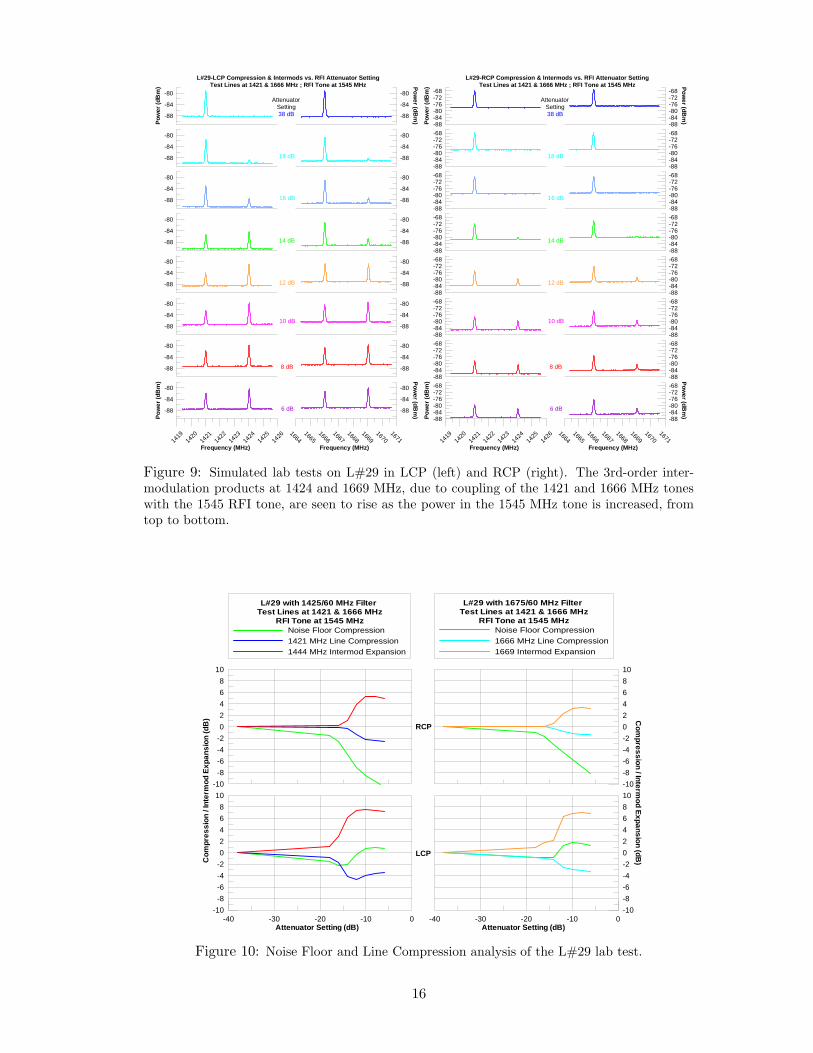
Figure 9 shows the results of a verification of the experiment concept that was carried out with a spareL-Band receiver (L#29) in a lab setting. Two Agilent 83630B synthesizers were used to simulate the1421 MHz (HI) and 1666 MHz (OH) spectral lines. The signals were combined with a splitter and feddirectly into the receiver through the quadridge OMT test fixture normally used to provide hot/coldnoise standards. An 83623L synthesizer provided the 3090 MHz RFI tone to the Hittite divide-by-2which was injected into the receiver using the noise calibration path, although in this case, throughthe solar cal path rather than the Pcal coupler as described above, thus providing 10 dB higher tonelevels for a given attenuator setting than were seen in the antenna tests performed later. The output ofthe receiver was measured with an Agilent 8563E spectrum analyzer which was configured to duplicatewhat the VLA correlator would see in spectral line mode with a 6.25 MHz bandwidth centered at1422.5 MHz or at 1667.5 MHz. The spectrum analyzer provides 601 spectral channels - many morethan the correlator has - with a 10.4 KHz spacing and a resolution bandwidth of 100 KHz.

Figure 9 shows the spectra at both the 1422.5 and 1667.5 MHz center frequencies for the LCP andRCP channels for various attenuator settings. The larger the attenuator value, the less power in the1545 MHz RFI tone. The traces at the top show the situation before any compression occurs. One cansee the simulated HI and OH lines at 1421 and 1666 MHz respectively in both channels. The strengthof these lines was set to be about 10 dB above the noise floor, which required a power level at the inputof the receiver of -101 dBm. As the power of the RFI tone increases, the third-order products beginto appear. The OH line is folded down to 1424 MHz (i.e., 2 × 1545 − 1666 = 1424 MHz) while the HIline is folded up to 1669 MHz (i.e., 2 × 1545 − 1421 = 1669 MHz). Note how the strength of both theHI and OH lines drop, as does the noise floor level (at least for a while), as the aliased lines grow inamplitude. It is also obvious that the LCP channel compresses before the RCP side does.

An Excel spreadsheet was used to calculate the average power in the noise floor around each of theprimary and folded lines, as well as to determine the maximum power of each of the four lines (withina (0.25 MHz window) for the various attenuator settings. Figure 10 shows a plot of the noise floorcompression ratio (green traces), the 1421 & 1666 MHz line compression (dark and light blue traces)and the 1444 & 1669 intermod line expansion (red & orange traces) with the LCP and RCP curvesshown separately.

On the RCP side, the noise floor drops steadily as the power of the injected RFI tone increases.The amplitudes of the 1421 and 1666 MHz simulated spectral lines also fall while the 1424 and 1669MHz intermod lines grow and eventually reach a plateau. All of these effects are expected on the basisof the analysis given in Sections 2, 3, and 4. However, on the LCP side, the noise floor initially dropsas tone power increases, but then begins to increase as the tone power reaches its highest levels. Inthe end, the noise floor had more average power than it started with. The 1421 and 1666 MHz linesdrop, and unlike the RCP channel, leveled off. The 1424 & 1669 MHz itermod lines stop growing andeventually plateau, much as they did on the RCP side.

The rising of the noise floor at high compression levels on the LCP channel came as a surprise. But

15

1419

1420

1421

1422

1423

1424

1425

1426

Frequency (MHz)

-88

-84

-80

Pow

er (d

Bm

)

AttenuatorSetting38 dB

18 dB

16 dB

14 dB

12 dB

10 dB

8 dB

6 dB

L#29-LCP Compression & Intermods vs. RFI Attenuator SettingTest Lines at 1421 & 1666 MHz ; RFI Tone at 1545 MHz

-88

-84

-80

-88

-84

-80

-88

-84

-80

-88

-84

-80

-88

-84

-80

-88

-84

-80

-88

-84

-80

Pow

er (d

Bm

)

16641665

16661667

16681669

16701671

Frequency (MHz)

-88

-84

-80

Pow

er (dBm

)

-88

-84

-80

-88

-84

-80

-88

-84

-80

-88

-84

-80

-88

-84

-80

-88

-84

-80

-88

-84

-80

Pow

er (dBm

)

1419

1420

1421

1422

1423

1424

1425

1426

Frequency (MHz)

-88-84-80-76-72-68

Pow

er (d

Bm

)

-88-84-80-76-72-68

-88-84-80-76-72-68

-88-84-80-76-72-68

-88-84-80-76-72-68

-88-84-80-76-72-68

-88-84-80-76-72-68

-88-84-80-76-72-68

Pow

er (d

Bm

)1664

16651666

16671668

16691670

1671Frequency (MHz)

-88-84-80-76-72-68

Pow

er (dBm

)

-88-84-80-76-72-68

-88-84-80-76-72-68

-88-84-80-76-72-68

-88-84-80-76-72-68

-88-84-80-76-72-68

-88-84-80-76-72-68

-88-84-80-76-72-68

Pow

er (dBm

)

AttenuatorSetting38 dB

18 dB

16 dB

14 dB

12 dB

10 dB

8 dB

6 dB

L#29-RCP Compression & Intermods vs. RFI Attenuator SettingTest Lines at 1421 & 1666 MHz ; RFI Tone at 1545 MHz

Figure 9: Simulated lab tests on L#29 in LCP (left) and RCP (right). The 3rd-order inter-modulation products at 1424 and 1669 MHz, due to coupling of the 1421 and 1666 MHz toneswith the 1545 RFI tone, are seen to rise as the power in the 1545 MHz tone is increased, fromtop to bottom.

-10

-8

-6

-4

-2

0

2

4

6

8

10

-10

-8

-6

-4

-2

0

2

4

6

8

10

-40 -30 -20 -10 0Attenuator Setting (dB)

-10

-8

-6

-4

-2

0

2

4

6

8

10

Com

pres

sion

/ In

term

od E

xpan

sion

(dB

)

L#29 with 1425/60 MHz Filter Test Lines at 1421 & 1666 MHz

RFI Tone at 1545 MHzNoise Floor Compression1421 MHz Line Compression1444 MHz Intermod Expansion

-40 -30 -20 -10 0Attenuator Setting (dB)

-10

-8

-6

-4

-2

0

2

4

6

8

10

Com

pression / Intermod E

xpansion (dB)

L#29 with 1675/60 MHz Filter Test Lines at 1421 & 1666 MHz

RFI Tone at 1545 MHzNoise Floor Compression1666 MHz Line Compression1669 Intermod Expansion

RCP

LCP

Figure 10: Noise Floor and Line Compression analysis of the L#29 lab test.

16

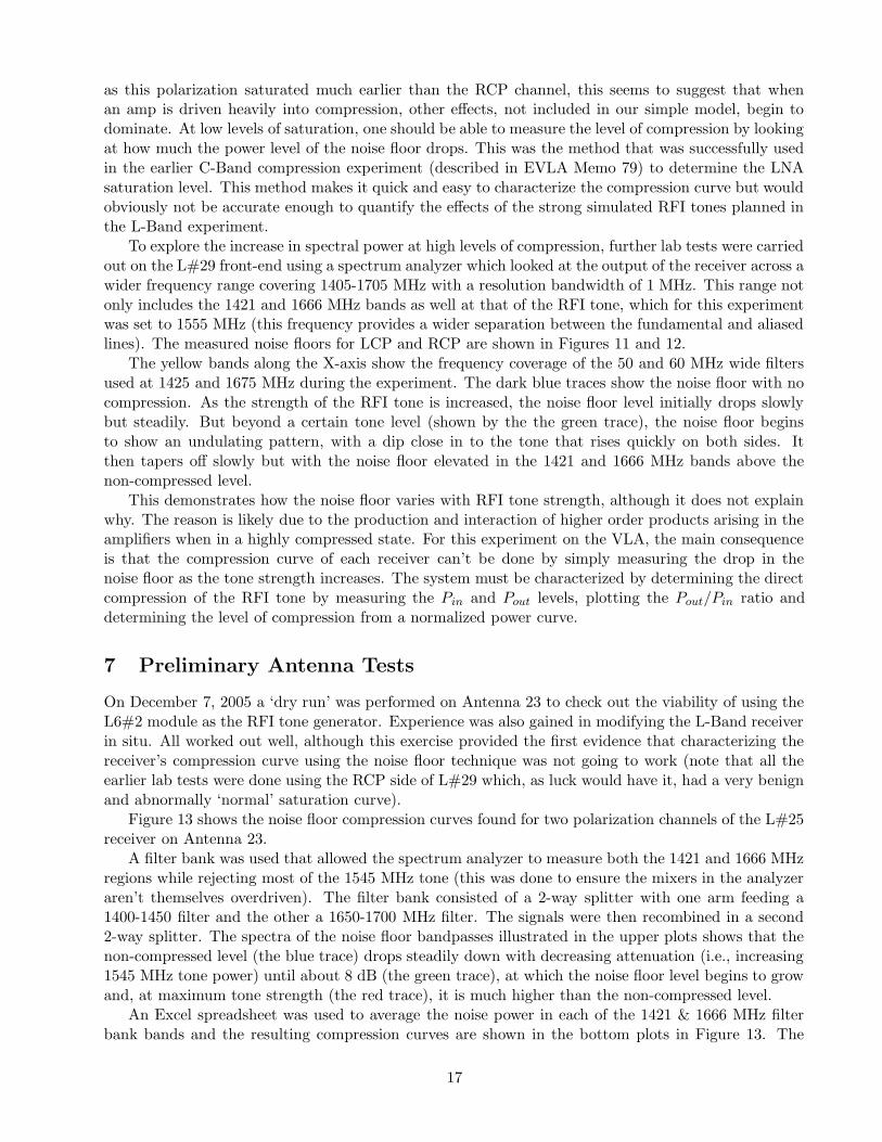
as this polarization saturated much earlier than the RCP channel, this seems to suggest that whenan amp is driven heavily into compression, other effects, not included in our simple model, begin todominate. At low levels of saturation, one should be able to measure the level of compression by lookingat how much the power level of the noise floor drops. This was the method that was successfully usedin the earlier C-Band compression experiment (described in EVLA Memo 79) to determine the LNAsaturation level. This method makes it quick and easy to characterize the compression curve but wouldobviously not be accurate enough to quantify the effects of the strong simulated RFI tones planned inthe L-Band experiment.

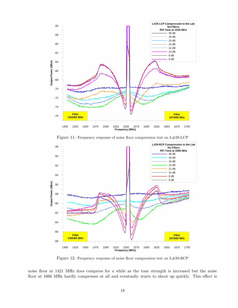
To explore the increase in spectral power at high levels of compression, further lab tests were carriedout on the L#29 front-end using a spectrum analyzer which looked at the output of the receiver across awider frequency range covering 1405-1705 MHz with a resolution bandwidth of 1 MHz. This range notonly includes the 1421 and 1666 MHz bands as well at that of the RFI tone, which for this experimentwas set to 1555 MHz (this frequency provides a wider separation between the fundamental and aliasedlines). The measured noise floors for LCP and RCP are shown in Figures 11 and 12.

The yellow bands along the X-axis show the frequency coverage of the 50 and 60 MHz wide filtersused at 1425 and 1675 MHz during the experiment. The dark blue traces show the noise floor with nocompression. As the strength of the RFI tone is increased, the noise floor level initially drops slowlybut steadily. But beyond a certain tone level (shown by the the green trace), the noise floor beginsto show an undulating pattern, with a dip close in to the tone that rises quickly on both sides. Itthen tapers off slowly but with the noise floor elevated in the 1421 and 1666 MHz bands above thenon-compressed level.

This demonstrates how the noise floor varies with RFI tone strength, although it does not explainwhy. The reason is likely due to the production and interaction of higher order products arising in theamplifiers when in a highly compressed state. For this experiment on the VLA, the main consequenceis that the compression curve of each receiver can’t be done by simply measuring the drop in thenoise floor as the tone strength increases. The system must be characterized by determining the directcompression of the RFI tone by measuring the Pin and Pout levels, plotting the Pout/Pin ratio anddetermining the level of compression from a normalized power curve.

7 Preliminary Antenna Tests

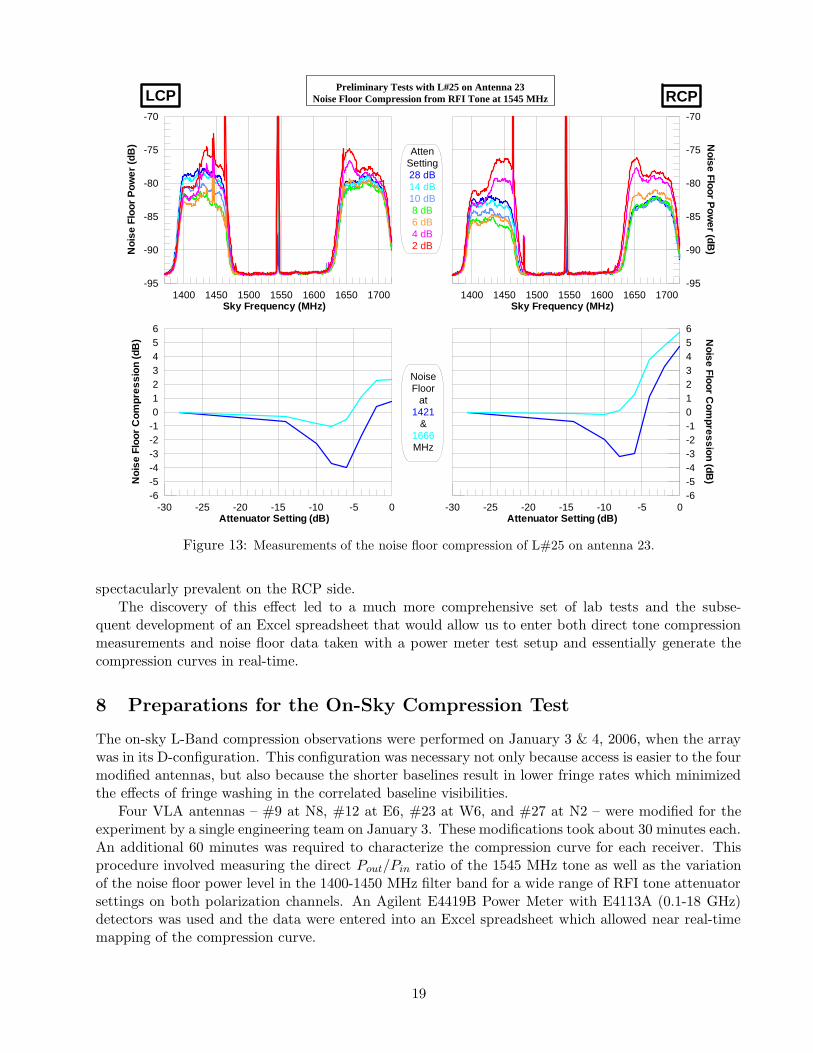
On December 7, 2005 a ‘dry run’ was performed on Antenna 23 to check out the viability of using theL6#2 module as the RFI tone generator. Experience was also gained in modifying the L-Band receiverin situ. All worked out well, although this exercise provided the first evidence that characterizing thereceiver’s compression curve using the noise floor technique was not going to work (note that all theearlier lab tests were done using the RCP side of L#29 which, as luck would have it, had a very benignand abnormally ‘normal’ saturation curve).

Figure 13 shows the noise floor compression curves found for two polarization channels of the L#25receiver on Antenna 23.

A filter bank was used that allowed the spectrum analyzer to measure both the 1421 and 1666 MHzregions while rejecting most of the 1545 MHz tone (this was done to ensure the mixers in the analyzeraren’t themselves overdriven). The filter bank consisted of a 2-way splitter with one arm feeding a1400-1450 filter and the other a 1650-1700 MHz filter. The signals were then recombined in a second2-way splitter. The spectra of the noise floor bandpasses illustrated in the upper plots shows that thenon-compressed level (the blue trace) drops steadily down with decreasing attenuation (i.e., increasing1545 MHz tone power) until about 8 dB (the green trace), at which the noise floor level begins to growand, at maximum tone strength (the red trace), it is much higher than the non-compressed level.

An Excel spreadsheet was used to average the noise power in each of the 1421 & 1666 MHz filterbank bands and the resulting compression curves are shown in the bottom plots in Figure 13. The

17

1400 1425 1450 1475 1500 1525 1550 1575 1600 1625 1650 1675 1700Frequency (MHz)

-76

-74

-72

-70

-68

-66

-64

-62

-60

-58

-56

Out

put P

ower

(dB

m)

L#29-LCP Compression in the LabNo Filters

RFI Tone at 1555 MHz38 dB18 dB16 dB14 dB12 dB10 dB8 dB6 dB

Filter1425/60 MHz

Filter1675/60 MHz

Figure 11: Frequency response of noise floor compression test on L#29-LCP

1400 1425 1450 1475 1500 1525 1550 1575 1600 1625 1650 1675 1700Frequency (MHz)

-68

-66

-64

-62

-60

-58

-56

-54

-52

-50

-48

Out

put P

ower

(dB

m)

L#29-RCP Compression in the LabNo Filters

RFI Tone at 1555 MHz38 dB18 dB16 dB14 dB12 dB10 dB8 dB6 dB

Filter1425/60 MHz

Filter1675/60 MHz

Figure 12: Frequency response of noise floor compression test on L#29-RCP

noise floor at 1421 MHz does compress for a while as the tone strength is increased but the noisefloor at 1666 MHz hardly compresses at all and eventually starts to shoot up quickly. This effect is

18

1400 1450 1500 1550 1600 1650 1700Sky Frequency (MHz)

-95

-90

-85

-80

-75

-70N

oise

Flo

or P

ower

(dB

)

AttenSetting28 dB14 dB10 dB8 dB6 dB4 dB2 dB

1400 1450 1500 1550 1600 1650 1700Sky Frequency (MHz)

-95

-90

-85

-80

-75

-70N

oise Floor Pow

er (dB)

-30 -25 -20 -15 -10 -5 0Attenuator Setting (dB)

-6-5-4-3-2-10123456

Noi

se F

loor

Com

pres

sion

(dB

)

Preliminary Tests with L#25 on Antenna 23Noise Floor Compression from RFI Tone at 1545 MHz

-30 -25 -20 -15 -10 -5 0Attenuator Setting (dB)

-6-5-4-3-2-10123456

Noise Floor C

ompression (dB

)LCP

NoiseFloor

at1421

&1666MHz

RCP

Figure 13: Measurements of the noise floor compression of L#25 on antenna 23.

spectacularly prevalent on the RCP side.The discovery of this effect led to a much more comprehensive set of lab tests and the subse-

quent development of an Excel spreadsheet that would allow us to enter both direct tone compressionmeasurements and noise floor data taken with a power meter test setup and essentially generate thecompression curves in real-time.

8 Preparations for the On-Sky Compression Test

The on-sky L-Band compression observations were performed on January 3 & 4, 2006, when the arraywas in its D-configuration. This configuration was necessary not only because access is easier to the fourmodified antennas, but also because the shorter baselines result in lower fringe rates which minimizedthe effects of fringe washing in the correlated baseline visibilities.

Four VLA antennas – #9 at N8, #12 at E6, #23 at W6, and #27 at N2 – were modified for theexperiment by a single engineering team on January 3. These modifications took about 30 minutes each.An additional 60 minutes was required to characterize the compression curve for each receiver. Thisprocedure involved measuring the direct Pout/Pin ratio of the 1545 MHz tone as well as the variationof the noise floor power level in the 1400-1450 MHz filter band for a wide range of RFI tone attenuatorsettings on both polarization channels. An Agilent E4419B Power Meter with E4113A (0.1-18 GHz)detectors was used and the data were entered into an Excel spreadsheet which allowed near real-timemapping of the compression curve.

19

In order to minimize any non-linear effects coming from the power detectors, a second step attenu-ator was used to adjust the strength of Pout so that it was nearly identical to the Pin level. Since a trueamplifier gain curve would require the detectors to be linear over many tens of dB, this scheme resultsin both Pin and Pout lying at the exact same operating point of the detectors so that the differentialnon-linearity is negligible. A 1500-1600 MHz filter is placed in front of the detector to eliminate mostof the noise power coming from the receiver. This ensures that we are predominately measuring theamplified 1545 MHz tone.

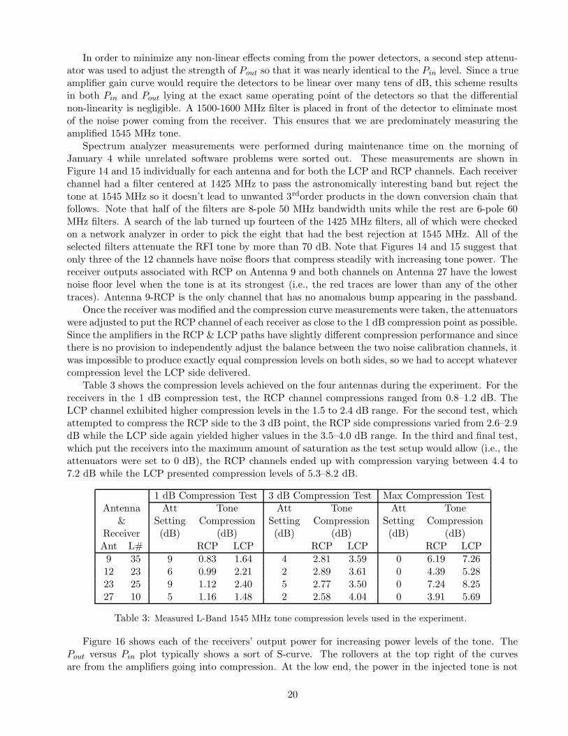
Spectrum analyzer measurements were performed during maintenance time on the morning ofJanuary 4 while unrelated software problems were sorted out. These measurements are shown inFigure 14 and 15 individually for each antenna and for both the LCP and RCP channels. Each receiverchannel had a filter centered at 1425 MHz to pass the astronomically interesting band but reject thetone at 1545 MHz so it doesn’t lead to unwanted 3rdorder products in the down conversion chain thatfollows. Note that half of the filters are 8-pole 50 MHz bandwidth units while the rest are 6-pole 60MHz filters. A search of the lab turned up fourteen of the 1425 MHz filters, all of which were checkedon a network analyzer in order to pick the eight that had the best rejection at 1545 MHz. All of theselected filters attenuate the RFI tone by more than 70 dB. Note that Figures 14 and 15 suggest thatonly three of the 12 channels have noise floors that compress steadily with increasing tone power. Thereceiver outputs associated with RCP on Antenna 9 and both channels on Antenna 27 have the lowestnoise floor level when the tone is at its strongest (i.e., the red traces are lower than any of the othertraces). Antenna 9-RCP is the only channel that has no anomalous bump appearing in the passband.

Once the receiver was modified and the compression curve measurements were taken, the attenuatorswere adjusted to put the RCP channel of each receiver as close to the 1 dB compression point as possible.Since the amplifiers in the RCP & LCP paths have slightly different compression performance and sincethere is no provision to independently adjust the balance between the two noise calibration channels, itwas impossible to produce exactly equal compression levels on both sides, so we had to accept whatevercompression level the LCP side delivered.

Table 3 shows the compression levels achieved on the four antennas during the experiment. For thereceivers in the 1 dB compression test, the RCP channel compressions ranged from 0.8–1.2 dB. TheLCP channel exhibited higher compression levels in the 1.5 to 2.4 dB range. For the second test, whichattempted to compress the RCP side to the 3 dB point, the RCP side compressions varied from 2.6–2.9dB while the LCP side again yielded higher values in the 3.5–4.0 dB range. In the third and final test,which put the receivers into the maximum amount of saturation as the test setup would allow (i.e., theattenuators were set to 0 dB), the RCP channels ended up with compression varying between 4.4 to7.2 dB while the LCP presented compression levels of 5.3–8.2 dB.

1 dB Compression Test 3 dB Compression Test Max Compression TestAntenna Att Tone Att Tone Att Tone

& Setting Compression Setting Compression Setting CompressionReceiver (dB) (dB) (dB) (dB) (dB) (dB)Ant L# RCP LCP RCP LCP RCP LCP

9 35 9 0.83 1.64 4 2.81 3.59 0 6.19 7.2612 23 6 0.99 2.21 2 2.89 3.61 0 4.39 5.2823 25 9 1.12 2.40 5 2.77 3.50 0 7.24 8.2527 10 5 1.16 1.48 2 2.58 4.04 0 3.91 5.69

Table 3: Measured L-Band 1545 MHz tone compression levels used in the experiment.

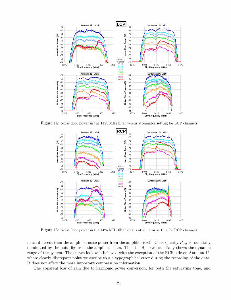
Figure 16 shows each of the receivers’ output power for increasing power levels of the tone. ThePout versus Pin plot typically shows a sort of S-curve. The rollovers at the top right of the curvesare from the amplifiers going into compression. At the low end, the power in the injected tone is not

20

1375 1400 1425 1450 1475Sky Frequency (MHz)

-89

-88

-87

-86

-85

-84

-83

-82

-81

-80

-79

Noi

se F

loor

Pow

er (d

B)

Antenna 09 / L#35

AttenSetting30 dB10 dB8 dB6 dB4 dB2 dB0 dB

1375 1400 1425 1450 1475Sky Frequency (MHz)

-78

-77

-76

-75

-74

-73

-72

-71

-70

-69

-68

Noi

se F

loor

Pow

er (d

B)

Antenna 12 / L#23

1375 1400 1425 1450 1475Sky Frequency (MHz)

-78

-77

-76

-75

-74

-73

-72

-71

-70

-69

-68

Noi

se F

loor

Pow

er (d

B)

Antenna 23 / L#25

1375 1400 1425 1450 1475Sky Frequency (MHz)

-94

-93

-92

-91

-90

-89

-88

-87

-86

-85

-84

Noi

se F

loor

Pow

er (d

B)

Antenna 27 / L#10

LCP

Figure 14: Noise floor power in the 1425 MHz filter versus attenuator setting for LCP channels

1375 1400 1425 1450 1475Sky Frequency (MHz)

-92

-91

-90

-89

-88

-87

-86

-85

-84

-83

-82

Noi

se F

loor

Pow

er (d

B)

Antenna 09 / L#35

AttenSetting30 dB10 dB8 dB6 dB4 dB2 dB0 dB

1375 1400 1425 1450 1475Sky Frequency (MHz)

-79

-78

-77

-76

-75

-74

-73

-72

-71

-70

-69

Noi

se F

loor

Pow

er (d

B)

Antenna 12 / L#23

1375 1400 1425 1450 1475Sky Frequency (MHz)

-90

-89

-88

-87

-86

-85

-84

-83

-82

-81

-80

Noi

se F

loor

Pow

er (d

B)

Antenna 23 / L#25

1375 1400 1425 1450 1475Sky Frequency (MHz)

-92

-91

-90

-89

-88

-87

-86

-85

-84

-83

-82

Noi

se F

loor

Pow

er (d

B)

Antenna 27 / L#10

RCP

Figure 15: Noise floor power in the 1425 MHz filter versus attenuator setting for RCP channels

much different than the amplified noise power from the amplifier itself. Consequently Pout is essentiallydominated by the noise figure of the amplifier chain. Thus the S-curve essentially shows the dynamicrange of the system. The curves look well behaved with the exception of the RCP side on Antenna 12,whose clearly discrepant point we ascribe to a a typographical error during the recording of the data.It does not affect the more important compression information.

The apparent loss of gain due to harmonic power conversion, for both the saturating tone, and

21

-70 -60 -50 -40 -30 -20 -10 0PIn (dBm)

-70

-60

-50

-40

-30

-20

-10

0

PO

ut (d

Bm

)

Antenna 09 / L#35

-70 -60 -50 -40 -30 -20 -10 0PIn (dBm)

-70

-60

-50

-40

-30

-20

-10

0

PO

ut (d

Bm

)

Antenna 12 / L#23

-70 -60 -50 -40 -30 -20 -10 0PIn (dBm)

-70

-60

-50

-40

-30

-20

-10

0

PO

ut (d

Bm

)

Antenna 23 / L#25

-70 -60 -50 -40 -30 -20 -10 0PIn (dBm)

-70

-60

-50

-40

-30

-20

-10

0

PO

ut (d

Bm

)

Antenna 27 / L#10

POut vs. PIn

RCPLCP

Figure 16: Measured Pout vs. Pin for the 1545 MHz tone.

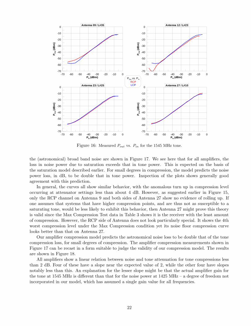
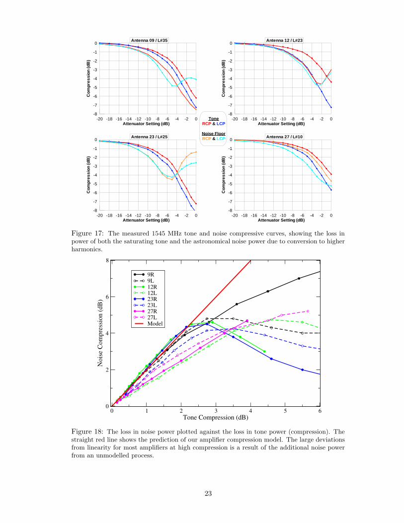
the (astronomical) broad band noise are shown in Figure 17. We see here that for all amplifiers, theloss in noise power due to saturation exceeds that in tone power. This is expected on the basis ofthe saturation model described earlier. For small degrees in compression, the model predicts the noisepower loss, in dB, to be double that in tone power. Inspection of the plots shows generally goodagreement with this prediction.

In general, the curves all show similar behavior, with the anomalous turn up in compression leveloccurring at attenuator settings less than about 4 dB. However, as suggested earlier in Figure 15,only the RCP channel on Antenna 9 and both sides of Antenna 27 show no evidence of rolling up. Ifone assumes that systems that have higher compression points, and are thus not as susceptible to asaturating tone, would be less likely to exhibit this behavior, then Antenna 27 might prove this theoryis valid since the Max Compression Test data in Table 3 shows it is the receiver with the least amountof compression. However, the RCP side of Antenna does not look particularly special. It shows the 4thworst compression level under the Max Compression condition yet its noise floor compression curvelooks better than that on Antenna 27.

Our amplifier compression model predicts the astronomical noise loss to be double that of the tonecompression loss, for small degrees of compression. The amplifier compression measurements shown inFigure 17 can be recast in a form suitable to judge the validity of our compression model. The resultsare shown in Figure 18.

All amplifiers show a linear relation between noise and tone attenuation for tone compressions lessthan 2 dB. Four of these have a slope near the expected value of 2, while the other four have slopesnotably less than this. An explanation for the lesser slope might be that the actual amplifier gain forthe tone at 1545 MHz is different than that for the noise power at 1425 MHz – a degree of freedom notincorporated in our model, which has assumed a single gain value for all frequencies.

22

-20 -18 -16 -14 -12 -10 -8 -6 -4 -2 0Attenuator Setting (dB)

-8

-7

-6

-5

-4

-3

-2

-1

0

Com

pres

sion

(dB

)

Antenna 09 / L#35

-20 -18 -16 -14 -12 -10 -8 -6 -4 -2 0Attenuator Setting (dB)

-8

-7

-6

-5

-4

-3

-2

-1

0

Com

pres

sion

(dB

)

Antenna 12 / L#23

-20 -18 -16 -14 -12 -10 -8 -6 -4 -2 0Attenuator Setting (dB)

-8

-7

-6

-5

-4

-3

-2

-1

0

Com

pres

sion

(dB

)

Antenna 23 / L#25

-20 -18 -16 -14 -12 -10 -8 -6 -4 -2 0Attenuator Setting (dB)

-8

-7

-6

-5

-4

-3

-2

-1

0

Com

pres

sion

(dB

)

Antenna 27 / L#10

ToneRCP & LCP

Noise FloorRCP & LCP

Figure 17: The measured 1545 MHz tone and noise compressive curves, showing the loss inpower of both the saturating tone and the astronomical noise power due to conversion to higherharmonics.

0 1 2 3 4 5 6Tone Compression (dB)

0

2

4

6

8

Noi

se C

ompr

essio

n (d

B)

9R9L12R12L23R23L27R27LModel

Figure 18: The loss in noise power plotted against the loss in tone power (compression). Thestraight red line shows the prediction of our amplifier compression model. The large deviationsfrom linearity for most amplifiers at high compression is a result of the additional noise powerfrom an unmodelled process.

23

9 The Astronomical Results

The on-sky observations were taken on the afternoon of 4 January, 2006. We observed the sourceW3OH, which includes both a strong (200 Jy) maser, and a strong (total flux of about 30Jy) continuumsource, allowing easy detection of HI in absorption. Observations were taken at the center frequenciesand resolution bandwidths given in Table 4.

Observational Setup

Freq. BW ∆ν Nch Mode Avg. CommentsMHz MHz kHz sec

1422.493 6.25 48.8 128 1A 6.7 Both HI and aliased OH in RCP1422.493 6.25 48.8 128 1C 6.7 Both HI and aliased OH in LCP1420.512 1.56 6.10 256 2AC 13.3 Centered on HI absorption1424.474 1.56 6.10 256 2AC 13.3 Centered on OH alias

Table 4: The observational setup

The observations were made both with the tone on and off, with the tone power set to put theamplifiers into approximately 1, 3 and 6 dB compression, as described in the preceding section. Theobservations at each of these levels took 48 minutes, including a calibration scan on 3C48 taken withthe tone ‘off’. Following the ‘1 dB’ and ‘3 dB’ observation blocks, the tone power attenuators wereadjusted to the values required for the next compression level, requiring approximately 20 minuteseach. Following the ‘6 dB’ observation block, all antennas were returned to their normal operatingstate.

The compression levels were measured in the field on the preceding day, and are given in Table 3.

9.1 Data Calibration

The data were calibrated using standard procedures. Observations of the calibrator source 3C48 (withthe saturating tone off) were used to determine the spectral bandpass, and to set the correct gain.3C48 is unresolved to the array resolution of ∼ 60 arcseconds, so no corrections for resolution wererequired. Data quality was excellent, and virtually no flagging of bad data was necessary.

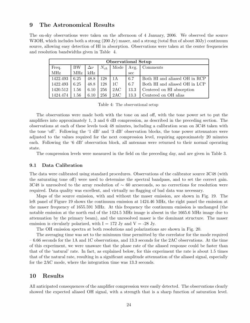
Maps of the source emission, with and without the maser emission, are shown in Fig. 19. Theleft panel of Figure 19 shows the continuum emission at 1424.46 MHz, the right panel the emission atthe maser frequency of 1655.591 MHz. At this frequency the continuum emission is unchanged (thenotable emission at the north end of the 1424.5 MHz image is absent in the 1665.6 MHz image due toattenuation by the primary beam), and the unresolved maser is the dominant structure. The maseremission is circularly polarized, with I = 172 Jy and V = -28 Jy.

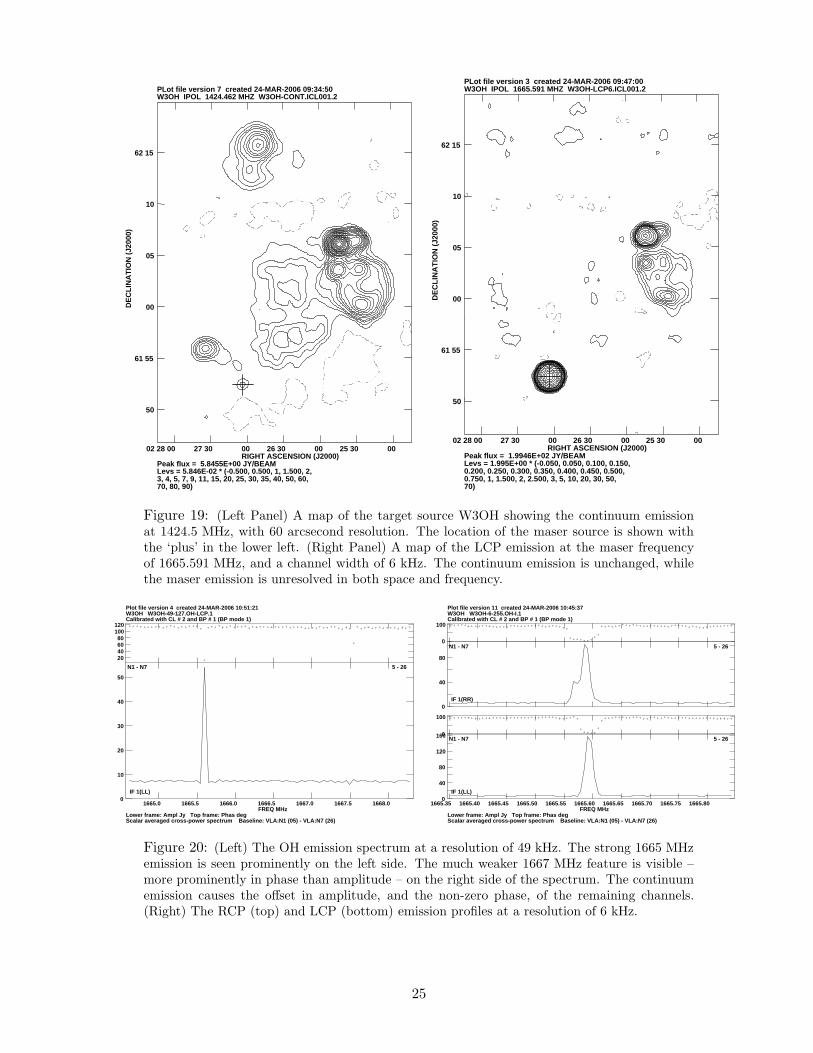
The OH emission spectra at both resolutions and polarizations are shown in Fig. 20.The averaging time was set to the minimum time permitted by the correlator for the mode required

– 6.66 seconds for the 1A and 1C observations, and 13.3 seconds for the 2AC observations. At the timeof this experiment, we were unaware that the phase rate of the aliased response could be faster thanthat of the ‘natural’ rate. In fact, as explained below, for this experiment the rate is about 1.5 timesthat of the natural rate, resulting in a significant amplitude attenuation of the aliased signal, especiallyfor the 2AC mode, where the integration time was 13.3 seconds.

10 Results

All anticipated consequences of the amplifier compression were easily detected. The observations clearlyshowed the expected aliased OH signal, with a strength that is a sharp function of saturation level.

24

W3OH IPOL 1424.462 MHZ W3OH-CONT.ICL001.2PLot file version 7 created 24-MAR-2006 09:34:50

Peak flux = 5.8455E+00 JY/BEAM Levs = 5.846E-02 * (-0.500, 0.500, 1, 1.500, 2,3, 4, 5, 7, 9, 11, 15, 20, 25, 30, 35, 40, 50, 60,70, 80, 90)

DE

CL

INA

TIO

N (

J200

0)

RIGHT ASCENSION (J2000)02 28 00 27 30 00 26 30 00 25 30 00

62 15

10

05

00

61 55

50

W3OH IPOL 1665.591 MHZ W3OH-LCP6.ICL001.2PLot file version 3 created 24-MAR-2006 09:47:00

Peak flux = 1.9946E+02 JY/BEAM Levs = 1.995E+00 * (-0.050, 0.050, 0.100, 0.150,0.200, 0.250, 0.300, 0.350, 0.400, 0.450, 0.500,0.750, 1, 1.500, 2, 2.500, 3, 5, 10, 20, 30, 50,70)

DE

CL

INA

TIO

N (

J200

0)

RIGHT ASCENSION (J2000)02 28 00 27 30 00 26 30 00 25 30 00

62 15

10

05

00

61 55

50

Figure 19: (Left Panel) A map of the target source W3OH showing the continuum emissionat 1424.5 MHz, with 60 arcsecond resolution. The location of the maser source is shown withthe ‘plus’ in the lower left. (Right Panel) A map of the LCP emission at the maser frequencyof 1665.591 MHz, and a channel width of 6 kHz. The continuum emission is unchanged, whilethe maser emission is unresolved in both space and frequency.

IF 1(LL)

FREQ MHz1665.0 1665.5 1666.0 1666.5 1667.0 1667.5 1668.0

50

40

30

20

10

0

12010080604020

Plot file version 4 created 24-MAR-2006 10:51:21W3OH W3OH-49-127.OH-LCP.1Calibrated with CL # 2 and BP # 1 (BP mode 1)

Lower frame: Ampl Jy Top frame: Phas degScalar averaged cross-power spectrum Baseline: VLA:N1 (05) - VLA:N7 (26)

N1 - N7 5 - 26

IF 1(RR)

80

40

0

100

0

Plot file version 11 created 24-MAR-2006 10:45:37W3OH W3OH-6-255.OH-I.1Calibrated with CL # 2 and BP # 1 (BP mode 1)

Lower frame: Ampl Jy Top frame: Phas degScalar averaged cross-power spectrum Baseline: VLA:N1 (05) - VLA:N7 (26)

N1 - N7 5 - 26

IF 1(LL)

FREQ MHz1665.35 1665.40 1665.45 1665.50 1665.55 1665.60 1665.65 1665.70 1665.75 1665.80

160

120

80

40

0

100

0N1 - N7 5 - 26

Figure 20: (Left) The OH emission spectrum at a resolution of 49 kHz. The strong 1665 MHzemission is seen prominently on the left side. The much weaker 1667 MHz feature is visible –more prominently in phase than amplitude – on the right side of the spectrum. The continuumemission causes the offset in amplitude, and the non-zero phase, of the remaining channels.(Right) The RCP (top) and LCP (bottom) emission profiles at a resolution of 6 kHz.

25

The phase of the aliased signal rotated as expected, and the visibility amplitudes of the non-aliasedsignal were reduced.

We discuss these in turn.

10.1 Coupling of Out-Of-Band Emission by Intermodulation

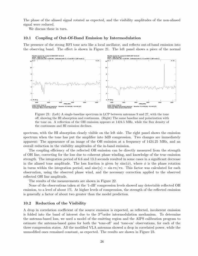
The presence of the strong RFI tone acts like a local oscillator, and reflects out-of-band emission intothe observing band. The effect is shown in Figure 21. The left panel shows a piece of the normal

IF 1(LL)

FREQ MHz1420 1421 1422 1423 1424 1425

12

10

8

6

4

2

0

Plot file version 22 created 14-MAR-2007 16:41:13W3OH 3DB-1C.LINE.1Freq = 1.4225 GHz, Bw = 6.250 MH Calibrated with CL # 2 and BP # 1 (BP mode 1)

Lower frame: Ampl JyScalar averaged cross-power spectrum Baseline: VLA:N8 (09) - VLA:N2 (27)Timerange: 00/21:17:40 to 00/21:18:33

8 - 2 9 - 27

IF 1(LL)

FREQ MHz1420 1421 1422 1423 1424 1425

12

10

8

6

4

2

0

Plot file version 23 created 14-MAR-2007 16:41:15W3OH 3DB-1C.LINE.1Freq = 1.4225 GHz, Bw = 6.250 MH Calibrated with CL # 2 and BP # 1 (BP mode 1)

Lower frame: Ampl JyScalar averaged cross-power spectrum Baseline: VLA:N8 (09) - VLA:N2 (27)Timerange: 00/21:18:53 to 00/21:19:53

8 - 2 9 - 27

Figure 21: (Left) A single-baseline spectrum in LCP between antennas 9 and 27, with the toneoff, showing the HI absorption and continuum. (Right) The same baseline and polarization withthe tone on. A reflection of the OH emission appears at 1424.5 MHz, while the flux density ofthe continuum and HI emission declines.

spectrum, with the HI absorption clearly visible on the left side. The right panel shows the emissionspectrum when the tone has put the amplifier into 3dB compression. Two changes are immediatelyapparent: The appearance of an image of the OH emission at a frequency of 1424.25 MHz, and anoverall reduction in the visibility amplitudes of the in-band emission.

The coupling efficiency of the reflected OH emission can be directly measured from the strengthof OH line, correcting for the loss due to coherent phase winding, and knowledge of the true emissionstrength. The integration period of 6.6 and 13.3 seconds resulted in some cases in a significant decreasein the aliased tone amplitude. The loss fraction is given by sinc(φ), where φ is the phase rotationin turns within the integration period, and sinc(x) = sinπx/πx. This factor was calculated for eachobservation, using the observed phase wind, and the necessary correction applied to the observedreflected OH line amplitude.

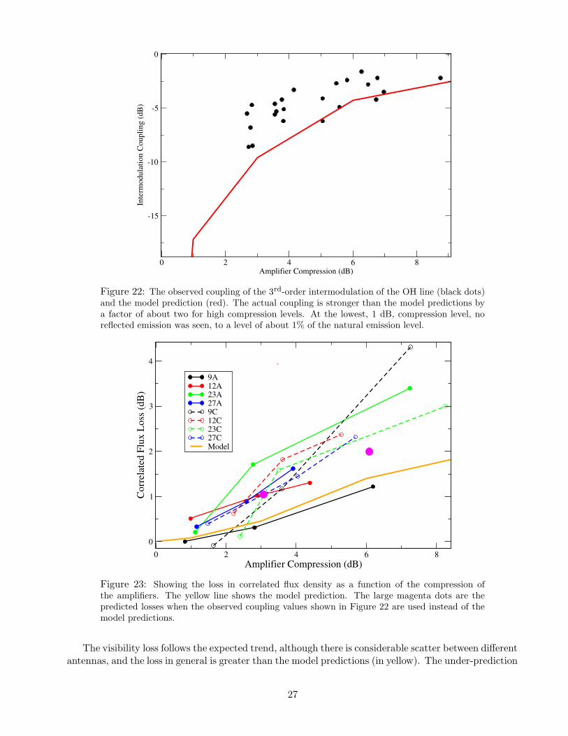
The results of the measurements are shown in Figure 22.None of the observations taken at the ‘1-dB’ compression levels showed any detectable reflected OH

emission, to a level of about 1%. At higher levels of compression, the strength of the reflected emissionis generally a factor of about two greater than the model prediction.

10.2 Reduction of the Visibility

A drop in correlation coefficient of the source emission is expected, as reflected, incoherent emissionis folded into the band of interest due to the 3rdorder intermodulation mechanism. To determinethe antenna-based loss, we used a model of the emitting region and the AIPS calibration program toestimate the antenna-based gains for both the ‘tone-off’ and ‘tone-on’ observations, for each of thethree compression states. All the modified VLA antennas showed a drop in correlated power, while theunmodified ones remained constant, as expected. The results are shown in Figure 23.

26

0 2 4 6 8Amplifier Compression (dB)

-15

-10

-5

0

Inte

rmod

ulat

ion

Coup

ling

(dB)

Figure 22: The observed coupling of the 3rd-order intermodulation of the OH line (black dots)and the model prediction (red). The actual coupling is stronger than the model predictions bya factor of about two for high compression levels. At the lowest, 1 dB, compression level, noreflected emission was seen, to a level of about 1% of the natural emission level.

0 2 4 6 8Amplifier Compression (dB)

0

1

2

3

4

Corre

late

d Fl

ux L

oss (

dB)

9A12A23A27A9C12C23C27CModel

Figure 23: Showing the loss in correlated flux density as a function of the compression ofthe amplifiers. The yellow line shows the model prediction. The large magenta dots are thepredicted losses when the observed coupling values shown in Figure 22 are used instead of themodel predictions.

The visibility loss follows the expected trend, although there is considerable scatter between differentantennas, and the loss in general is greater than the model predictions (in yellow). The under-prediction

27

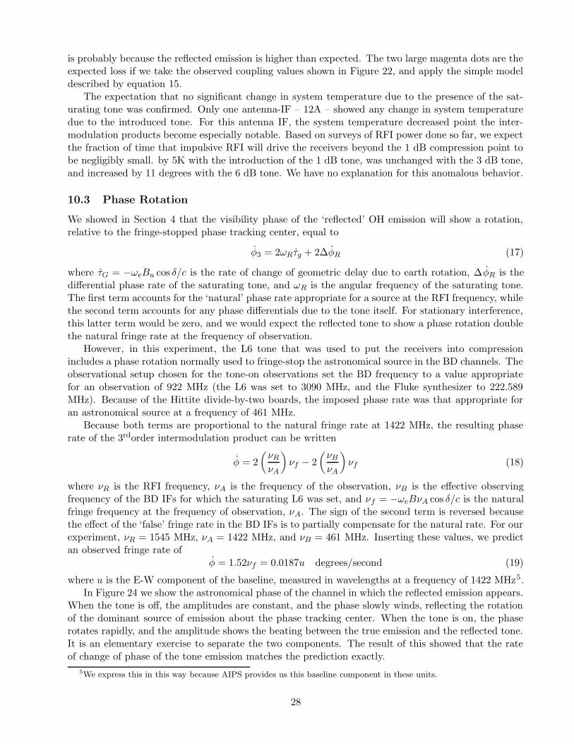
is probably because the reflected emission is higher than expected. The two large magenta dots are theexpected loss if we take the observed coupling values shown in Figure 22, and apply the simple modeldescribed by equation 15.

The expectation that no significant change in system temperature due to the presence of the sat-urating tone was confirmed. Only one antenna-IF – 12A – showed any change in system temperaturedue to the introduced tone. For this antenna IF, the system temperature decreased point the inter-modulation products become especially notable. Based on surveys of RFI power done so far, we expectthe fraction of time that impulsive RFI will drive the receivers beyond the 1 dB compression point tobe negligibly small. by 5K with the introduction of the 1 dB tone, was unchanged with the 3 dB tone,and increased by 11 degrees with the 6 dB tone. We have no explanation for this anomalous behavior.

10.3 Phase Rotation

We showed in Section 4 that the visibility phase of the ‘reflected’ OH emission will show a rotation,relative to the fringe-stopped phase tracking center, equal to

φ̇3 = 2ωRτ̇g + 2∆φ̇R (17)

where τ̇G = −ωeBu cos δ/c is the rate of change of geometric delay due to earth rotation, ∆φ̇R is thedifferential phase rate of the saturating tone, and ωR is the angular frequency of the saturating tone.The first term accounts for the ‘natural’ phase rate appropriate for a source at the RFI frequency, whilethe second term accounts for any phase differentials due to the tone itself. For stationary interference,this latter term would be zero, and we would expect the reflected tone to show a phase rotation doublethe natural fringe rate at the frequency of observation.

However, in this experiment, the L6 tone that was used to put the receivers into compressionincludes a phase rotation normally used to fringe-stop the astronomical source in the BD channels. Theobservational setup chosen for the tone-on observations set the BD frequency to a value appropriatefor an observation of 922 MHz (the L6 was set to 3090 MHz, and the Fluke synthesizer to 222.589MHz). Because of the Hittite divide-by-two boards, the imposed phase rate was that appropriate foran astronomical source at a frequency of 461 MHz.

Because both terms are proportional to the natural fringe rate at 1422 MHz, the resulting phaserate of the 3rdorder intermodulation product can be written

φ̇ = 2

(

νR

νA

)

νf − 2

(

νB

νA

)

νf (18)

where νR is the RFI frequency, νA is the frequency of the observation, νB is the effective observingfrequency of the BD IFs for which the saturating L6 was set, and νf = −ωeBνA cos δ/c is the naturalfringe frequency at the frequency of observation, νA. The sign of the second term is reversed becausethe effect of the ‘false’ fringe rate in the BD IFs is to partially compensate for the natural rate. For ourexperiment, νR = 1545 MHz, νA = 1422 MHz, and νB = 461 MHz. Inserting these values, we predictan observed fringe rate of

φ̇ = 1.52νf = 0.0187u degrees/second (19)

where u is the E-W component of the baseline, measured in wavelengths at a frequency of 1422 MHz5.In Figure 24 we show the astronomical phase of the channel in which the reflected emission appears.

When the tone is off, the amplitudes are constant, and the phase slowly winds, reflecting the rotationof the dominant source of emission about the phase tracking center. When the tone is on, the phaserotates rapidly, and the amplitude shows the beating between the true emission and the reflected tone.It is an elementary exercise to separate the two components. The result of this showed that the rateof change of phase of the tone emission matches the prediction exactly.

5We express this in this way because AIPS provides us this baseline component in these units.

28

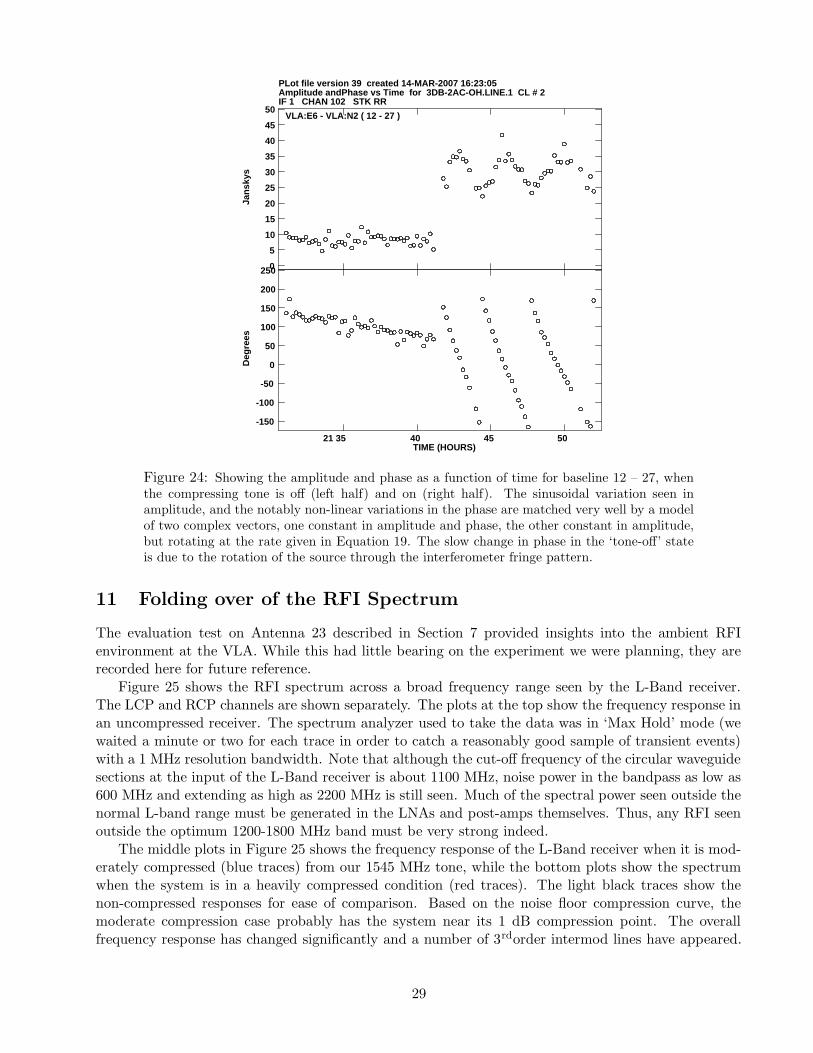
IF 1 CHAN 102 STK RRAmplitude andPhase vs Time for 3DB-2AC-OH.LINE.1 CL # 2PLot file version 39 created 14-MAR-2007 16:23:05

Jan

skys

50

45

40

35

30

25

20

15

10

5

0

VLA:E6 - VLA:N2 ( 12 - 27 )

Deg

rees

TIME (HOURS)21 35 40 45 50

250

200

150

100

50

0

-50

-100

-150

Figure 24: Showing the amplitude and phase as a function of time for baseline 12 – 27, whenthe compressing tone is off (left half) and on (right half). The sinusoidal variation seen inamplitude, and the notably non-linear variations in the phase are matched very well by a modelof two complex vectors, one constant in amplitude and phase, the other constant in amplitude,but rotating at the rate given in Equation 19. The slow change in phase in the ‘tone-off’ stateis due to the rotation of the source through the interferometer fringe pattern.

11 Folding over of the RFI Spectrum

The evaluation test on Antenna 23 described in Section 7 provided insights into the ambient RFIenvironment at the VLA. While this had little bearing on the experiment we were planning, they arerecorded here for future reference.

Figure 25 shows the RFI spectrum across a broad frequency range seen by the L-Band receiver.The LCP and RCP channels are shown separately. The plots at the top show the frequency response inan uncompressed receiver. The spectrum analyzer used to take the data was in ‘Max Hold’ mode (wewaited a minute or two for each trace in order to catch a reasonably good sample of transient events)with a 1 MHz resolution bandwidth. Note that although the cut-off frequency of the circular waveguidesections at the input of the L-Band receiver is about 1100 MHz, noise power in the bandpass as low as600 MHz and extending as high as 2200 MHz is still seen. Much of the spectral power seen outside thenormal L-band range must be generated in the LNAs and post-amps themselves. Thus, any RFI seenoutside the optimum 1200-1800 MHz band must be very strong indeed.

The middle plots in Figure 25 shows the frequency response of the L-Band receiver when it is mod-erately compressed (blue traces) from our 1545 MHz tone, while the bottom plots show the spectrumwhen the system is in a heavily compressed condition (red traces). The light black traces show thenon-compressed responses for ease of comparison. Based on the noise floor compression curve, themoderate compression case probably has the system near its 1 dB compression point. The overallfrequency response has changed significantly and a number of 3rdorder intermod lines have appeared.

29

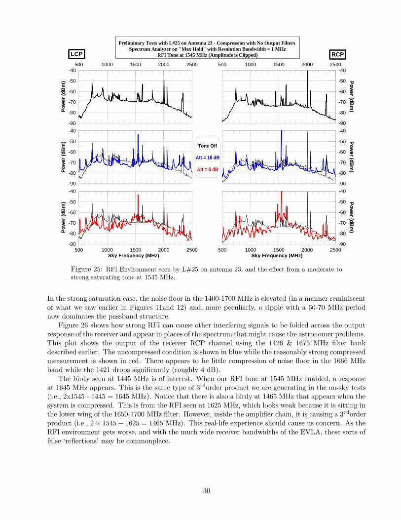
-90

-80

-70

-60

-50

-40

Pow

er (d

Bm

)500 1000 1500 2000 2500

Tone Off

Att = 16 dB

Att = 6 dB

500 1000 1500 2000 2500Sky Frequency (MHz)

-90

-80

-70

-60

-50

-40

Pow

er (d

Bm

)

Preliminary Tests with L#25 on Antenna 23 - Compression with No Output Filters Spectrum Analyzer on "Max Hold" with Resolution Bandwidth = 1 MHz

RFI Tone at 1545 MHz (Amplitude is Clipped)LCP

-90

-80

-70

-60

-50

-40

Pow

er (d

Bm

)500 1000 1500 2000 2500

-90

-80

-70

-60

-50

-40

Pow

er (dBm

)

500 1000 1500 2000 2500Sky Frequency (MHz)

-90

-80

-70

-60

-50

-40

Pow

er (dBm

)

-90

-80

-70

-60

-50

-40

Pow

er (dBm

)RCP

Figure 25: RFI Environment seen by L#25 on antenna 23, and the effect from a moderate tostrong saturating tone at 1545 MHz.

In the strong saturation case, the noise floor in the 1400-1700 MHz is elevated (in a manner reminiscentof what we saw earlier in Figures 11and 12) and, more peculiarly, a ripple with a 60-70 MHz periodnow dominates the passband structure.

Figure 26 shows how strong RFI can cause other interfering signals to be folded across the outputresponse of the receiver and appear in places of the spectrum that might cause the astronomer problems.This plot shows the output of the receiver RCP channel using the 1426 & 1675 MHz filter bankdescribed earlier. The uncompressed condition is shown in blue while the reasonably strong compressedmeasurement is shown in red. There appears to be little compression of noise floor in the 1666 MHzband while the 1421 drops significantly (roughly 4 dB).

The birdy seen at 1445 MHz is of interest. When our RFI tone at 1545 MHz enabled, a responseat 1645 MHz appears. This is the same type of 3rdorder product we are generating in the on-sky tests(i.e., 2x1545 - 1445 = 1645 MHz). Notice that there is also a birdy at 1465 MHz that appears when thesystem is compressed. This is from the RFI seen at 1625 MHz, which looks weak because it is sitting inthe lower wing of the 1650-1700 MHz filter. However, inside the amplifier chain, it is causing a 3rdorderproduct (i.e., 2 × 1545 − 1625 = 1465 MHz). This real-life experience should cause us concern. As theRFI environment gets worse, and with the much wide receiver bandwidths of the EVLA, these sorts offalse ‘reflections’ may be commonplace.

30

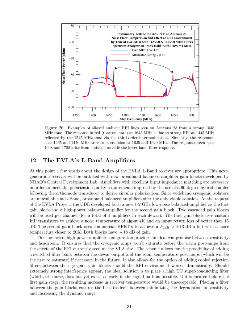
20

1350 1400 1450 1500 1550 1600 1650 1700Sky Frequency (MHz)

-100

-90

-80

-70

-60

-50

Noi

se F

loor

Pow

er (

dB

m)

Preliminary Tests with L#25-RCP on Antenna 23Noise Floor Compression and Effect on RFI Environmentby Tone at 1545 MHz with 1425/50 & 1675/50 MHz FiltersSpectrum Analyzer on "Max Hold" with RBW = 1 MHz

1545 MHz Tone OffAttenuator Setting = 8 dB

Figure 26: Examples of aliased ambient RFI lines seen on Antenna 23 from a strong 1545MHz tone. The response in red (tone-on state) at 1645 MHz is due to strong RFI at 1445 MHzreflected by the 1545 MHz tone via the third-order intermodulation. Similarly, the responsesnear 1465 and 1470 MHz arise from emission at 1625 and 1620 MHz. The responses seen near1698 and 1708 arise from emission outside the lower band filter response.

12 The EVLA’s L-Band Amplifiers

At this point a few words about the design of the EVLA L-Band receiver are appropriate. This next-generation receiver will be outfitted with new broadband balanced-amplifier gain blocks developed byNRAO’s Central Development Lab. Amplifiers with excellent input impedance matching are necessaryin order to meet the polarization purity requirements imposed by the use of a 90-degree hybrid couplerfollowing the orthomode transducer to derive circular polarization. Since wideband cryogenic isolatorsare unavailable at L-Band, broadband balanced amplifiers offer the only viable solution. At the requestof the EVLA Project, the CDL developed both a new 1-2 GHz low-noise balanced-amplifier as the firstgain block and a high-power balanced-amplifier for the second gain block. Two cascaded gain blockswill be used per channel (for a total of 4 amplifiers in each dewar). The first gain block uses customInP transistors to achieve a noise temperature of about 4K and an input return loss of better than 15dB. The second gain block uses commercial HFET’s to achieve a P1dB > +13 dBm but with a noisetemperature closer to 20K. Both blocks have ∼ 18 dB of gain.

This low-noise, high-power amplifier configuration provides an ideal compromise between sensitivityand headroom. It ensures that the cryogenic amps won’t saturate before the warm post-amps fromthe effects of the RFI currently seen at the VLA site. The scheme allows for the possibility of addinga switched filter bank between the dewar output and the room temperature post-amps (which will bethe first to saturate) if necessary in the future. It also allows for the option of adding cooled rejectionfilters between the cryogenic gain blocks should the RFI environment worsen dramatically. Shouldextremely strong interference appear, the ideal solution is to place a high TC super-conducting filter(which, of course, does not yet exist) as early in the signal path as possible. If it is located before thefirst gain stage, the resulting increase in receiver temperature would be unacceptable. Placing a filterbetween the gain blocks ensures the best tradeoff between minimizing the degradation in sensitivityand increasing the dynamic range.

31

Eight EVLA interim L-Band receivers have been built as of April 2007 and are placed on the EVLAantennas. These are existing VLA systems that have been modified with the octave bandwidth gainblocks along with a hybrid coupler circular polarizer. Seven if these retain the old VLA narrowband1.2-1.8 GHz orthomode transducer, but nevertheless allow us to characterize the performance expectedfrom the final EVLA version. In December 2004, compression tests were carried out on a VLA L-Bandreceiver (L#11), which utilized old-style cooled single-ended amplifiers, and the first receiver (L#32)to be outfitted with the balanced-amplifier blocks. The 1 dB compression point was measured for eachreceiver using a swept CW signal. Without the warm post-amps, while L#11 had an input saturationpower level of -34 dBm while L#32 had -22 dBm – 12 dB improvement in headroom. With the post-amps included, L#11 saturated at -48 dBm and L#32 at -47 dBm, which indicates that the post-ampsare the limiting factor. It turns out that these 1.2-1.8 GHz amps are surprisingly weak, with a P1dBpoint of only about -5 dBm). The new EVLA receiver design will utilize higher power post-amps witha P1dB > +15 dBm.

In order to avoid the adverse affects of non-linearities which may arise in amplifiers, mixers, ordiode attenuators that are driven into compression, the design of all the EVLA front-ends, and thesubsequent IF modules in the signal path, attempts to ensure that the standard operating point (i.e.,the power level when observing ‘cold’ sky) is well below the saturation point of any active device.This is a delicate balance since the signal must also be well above the noise floor of the variousamplifiers in the RF/IF chain to ensure the overall system temperature is not degraded. The headroomspecification in the EVLA Project Book calls for all the active components to be operating at least20 dB below their 1% compression point (which corresponds to being about 32 dB below their 1 dBcompression point). The major impact of insufficient headroom will only become a major limitation inthe presence of strong interference, where unwanted harmonics and intermodulation products generatedin the amplifiers and mixers may cause spurious signals to arise. The 20 dB headroom spec shouldprovide adequate dynamic range to mitigate the effects of both existing and future RFI. By utilizinghigh-power cryogenic balanced-amplifiers and post-amps, the new EVLA L-Band receiver system willachieve a much improved headroom specification over the existing VLA front-end. When looking atcold sky, the EVLA receiver should have over 40 dB of headroom. Interference like the DME signalsfrom airplanes, which are expected to increase the instantaneous integrated power seen in the 1-2 GHzband by about 20 dB, should be handled comfortably by the receiver. Evidence that this is so comesfrom EVLA antenna 14, which has the prototype OMT installed, thus exposing the amplifiers to thefull range of the aernautical band’s signals. Comparison of this antenna’s sensitivity and performancein the standard observing bands with that existing prior to the installation of the new OMT has shownno notable change.

13 Summary

We have conducted a carefully calibrated experiment in which four VLA L-band receivers were putinto known degrees of amplifier compression by the introduction of a noise tone at 1545 MHz. Theresulting compression reflects, via the third-order intermodulation mechanism, the strong OH maseremission at 1665 MHz to a frequency of 1425 MHz, adjacent to the HI absorption line.

We have measured the degree of coupling of this reflection mechanism through astronomical obser-vations of W3OH, an object which contains both a strong OH maser, and a nearby continuum source,in front of which lies neutral HI. The observations show the coupling efficiency of the intermodulationrises sharply with degree of compression, such that at 1 dB compression, the reflected emission is seenat ∼1% of its true intensity, while by 3 dB compression, it has reached ∼25% of actual strength.

The third-order intermodulation mechanism introduces a phase coupling into the reflected signalwhich, for a non-moving external saturating signal, will cause the interferometer phase of the reflectedsignal to rotate, relative to the astronomical source of interest, at twice the natural fringe rate. This rel-

32

atively fast rotation is very useful in decorrelating the reflected emission, and preventing the appearanceof a ‘ghost’ image of the reflected emission into the desired image.

The reflected signal, however, will introduce extra noise, resulting in a reduction of the correlationcoefficient of the desired emission. This reduction cannot be recovered by normal system temperaturecalibration methods, as the reflected signal has the synchronous calibration noise embedded. The losscould be corrected through normal off-source calibration, provided the saturation is unchanged betweencalibrator and target.

The saturating signal converts power out of the fundamental frequency into higher harmonics,resulting in an effective loss of gain for both the tone power and the astronomical power. Curiously,the loss for (assumed weak) astronomical power is as high as twice that of the tone power. This gainloss in noise power would be automatically corrected for by standard gain stabilization techniques,provided the saturating signal is stable over the integration time of the gain monitors. This situation,however, is unlikely to pertain for most observations, where the RFI is sporadic and/or highly timevariable. In this case, the reduction of gain will be uncompensated for, and a potentially large loss inapparent interferometer visibility will result.

The best defense against these RFI-induced effects is to design radio astronomical amplifier systemsto provide the largest possible range between the cold-sky operating power and the 1-dB compressionpoint, which is where the amplitude scale errors become truly noticeable. It is noted that higher head-room must inevitably be traded off against better sensitivity, so that knowledge of the expected RFIpower spectrum is essential for optimum design of the amplifier chain. The goal must be to design thesystem so that the head-room is set such that a negligible fraction of the observing time is spent in astate of compression exceed ∼1 dB.

The EVLA L-band design has incorporated these goals and constraints. Initial tests with the firstantenna to be outfitted with the new wide-band OMT shows no noticeable loss in sensitivity.

14 Acknowledgements

This experiment was facilitated by the expert assistance of Brent Willoughby and John McClenden.We thank Tanner Oates for his software for capture spectrum analyzer data. We are especially gratefulfor the assistance provided by Dan Mertely in outfitting, calibrating and adjusting the four modifiedantennas, and for the discussions held with Ken Sowinski, which were instrumental in understandingsome of the interesting phenomena generated by this experiment.

References

[1] Rick Perley. EVLA Memorandum #66, The Effect of Electronics Non-Linearity on Closure andImaging. August 2003

[2] Rick Perley and Bob Hayward. EVLA Memorandum #79, The Effect of Strong CW Signals onInterferometer Calibration, Closure, and Imaging. July 2004

[3] A. Harris. ALMA Memorandum #307, Precision Radiometry and the APHID 22 GHz Water lineMonitor. May 2000

33