Methodology

In our study the main thing is that we are using Box-Jenkins methodology. The basis of the Box-Jenkins modelling approach consists of three main stages which are the first one model identification, second one model estimation and validation and the last one is model application.

Model Identification

The first step in the Box-Jenkins is to identify the class of model most suitable to be applied to the given data set. Common statistics used to identify the model type are the autocorrelation and the partial autocorrelation.

The process of identifying the models is as follows:

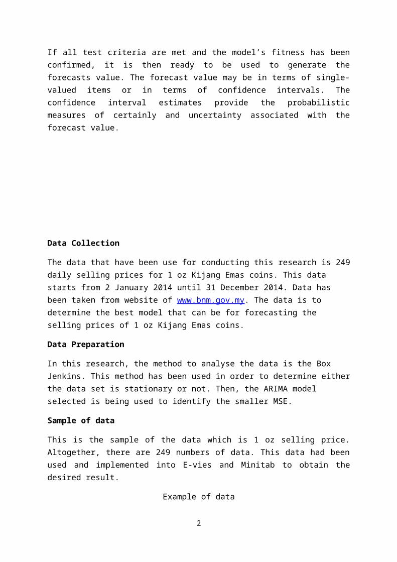
I. In step one, is to compute and analyse the various statistics based on the historical data, in particular the ACF and PACF.

II. Secondly, based on information obtained from I, the most suitable subclass of general model is then identified.

Model Estimation and Diagnostic Testing

There are two important objectives that need to be achieved when fitting the model are:

I. The fitted values should be as close as possible to actual values.II. The models should require the least possible parameters consistent with a ‘good’

model fit.

The first objectives concern the general fitness of the model. A model fits the data well if it satisfies certain statistical criteria. This is done by firstly, estimating the parameters and secondly generating the estimated values. The specific parameter values are estimated subject to the condition that the selected error measure is minimised.

Model application

If all test criteria are met and the model’s fitness has been confirmed, it is then ready to be used to generate the forecasts value. The forecast value may be in terms of single-valued items or in terms of confidence intervals. The confidence interval estimates provide the probabilistic measures of certainly and uncertainty associated with the forecast value.

1

Data Collection

The data that have been use for conducting this research is 249 daily selling prices for 1 oz Kijang Emas coins. This data starts from 2 January 2014 until 31 December 2014. Data has been taken from website of www.bnm.gov.my. The data is to determine the best model that can be for forecasting the selling prices of 1 oz Kijang Emas coins.

Data Preparation

In this research, the method to analyse the data is the Box Jenkins. This method has been used in order to determine either the data set is stationary or not. Then, the ARIMA model selected is being used to identify the smaller MSE.

Sample of data

This is the sample of the data which is 1 oz selling price. Altogether, there are 249 numbers of data. This data had been used and implemented into E-vies and Minitab to obtain the desired result.

Example of data

2

Result and Analysis

Estimation Part

Figure 1: Unit Root Test

3

Figure 2: Unit Root Test for First Differencing

4

Figure 3: Correlogram

5

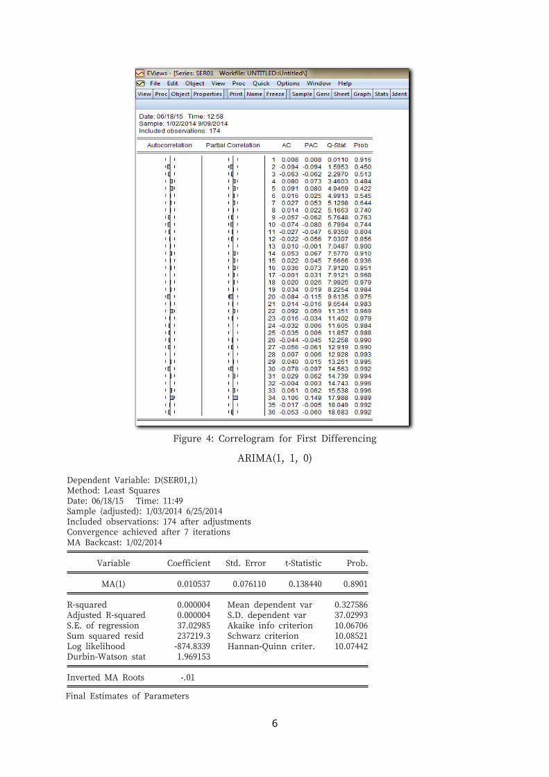
Figure 4: Correlogram for First Differencing

ARIMA(1, 1, 0)

Dependent Variable: D(SER01,1)Method: Least SquaresDate: 06/18/15 Time: 11:49Sample (adjusted): 1/03/2014 6/25/2014Included observations: 174 after adjustmentsConvergence achieved after 7 iterationsMA Backcast: 1/02/2014

Variable Coefficient Std. Error t-Statistic Prob.

MA(1) 0.010537 0.076110 0.138440 0.8901

R-squared 0.000004    Mean dependent var 0.327586Adjusted R-squared 0.000004    S.D. dependent var 37.02993S.E. of regression 37.02985    Akaike info criterion 10.06706Sum squared resid 237219.3    Schwarz criterion 10.08521Log likelihood -874.8339    Hannan-Quinn criter. 10.07442Durbin-Watson stat 1.969153

Inverted MA Roots      -.01

Final Estimates of Parameters

6

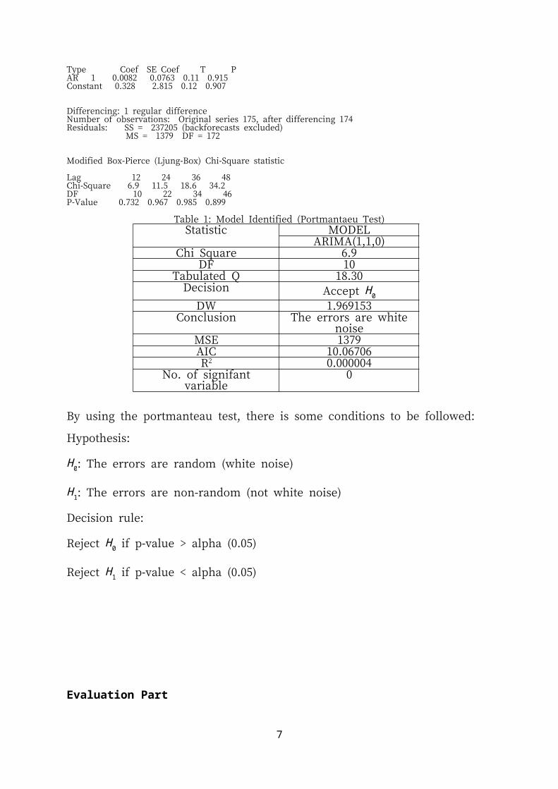
Type Coef SE Coef T PAR 1 0.0082 0.0763 0.11 0.915Constant 0.328 2.815 0.12 0.907

Differencing: 1 regular differenceNumber of observations: Original series 175, after differencing 174Residuals: SS = 237205 (backforecasts excluded) MS = 1379 DF = 172

Modified Box-Pierce (Ljung-Box) Chi-Square statistic

Lag 12 24 36 48Chi-Square 6.9 11.5 18.6 34.2DF 10 22 34 46P-Value 0.732 0.967 0.985 0.899

Table 1: Model Identified (Portmantaeu Test)

Statistic MODELARIMA(1,1,0)

Chi Square 6.9DF 10

Tabulated Q 18.30Decision Accept H 0

DW 1.969153Conclusion The errors are white noise

MSE 1379AIC 10.06706R2 0.000004

No. of signifant variable 0

By using the portmanteau test, there is some conditions to be followed:

Hypothesis:

H 0: The errors are random (white noise)

H 1: The errors are non-random (not white noise)

Decision rule:

Reject H 0 if p-value > alpha (0.05)

Reject H 1 if p-value < alpha (0.05)

7

Evaluation Part

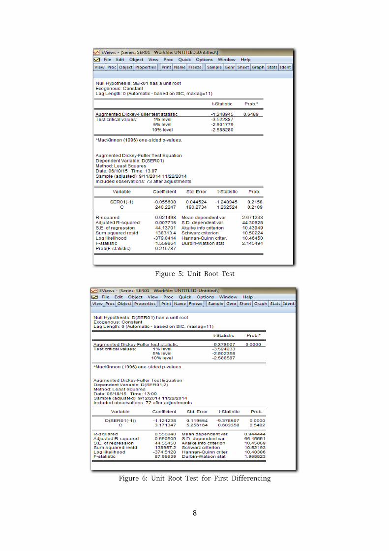
Figure 5: Unit Root Test

Figure 6: Unit Root Test for First Differencing

8

Figure 7: Correlogram

9

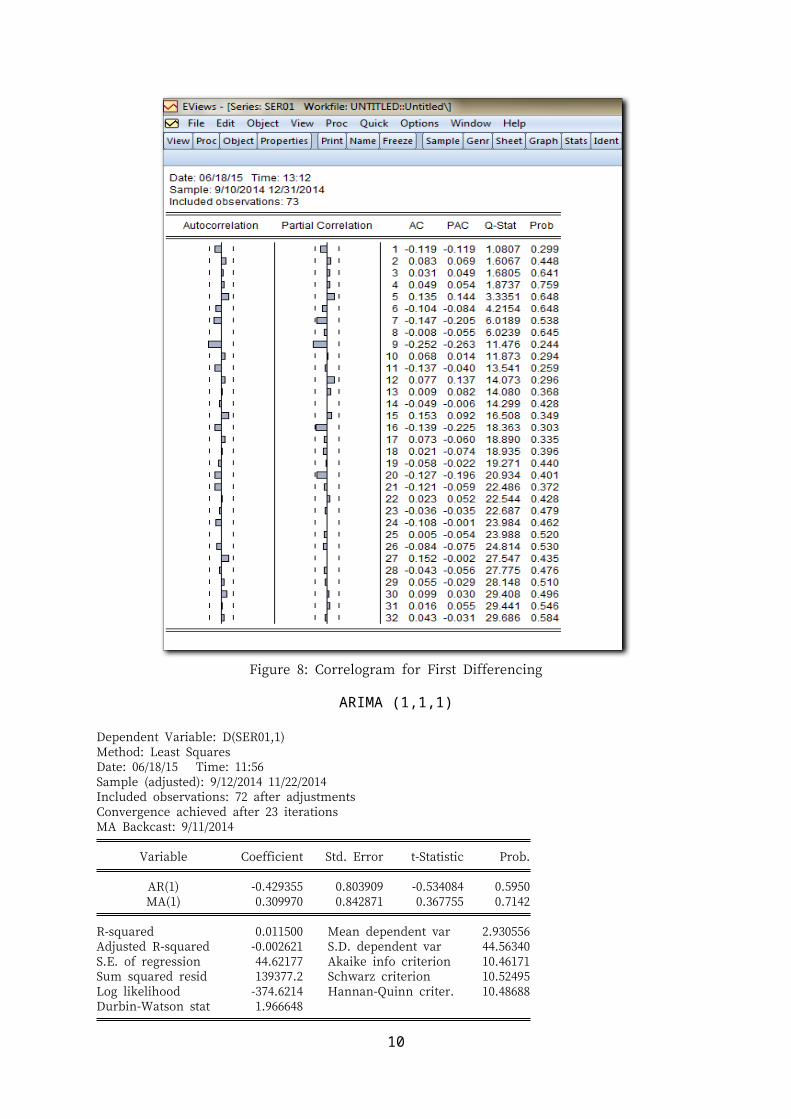
Figure 8: Correlogram for First Differencing

ARIMA (1,1,1)

Dependent Variable: D(SER01,1)Method: Least SquaresDate: 06/18/15 Time: 11:56Sample (adjusted): 9/12/2014 11/22/2014Included observations: 72 after adjustmentsConvergence achieved after 23 iterationsMA Backcast: 9/11/2014

Variable Coefficient Std. Error t-Statistic Prob.

AR(1) -0.429355 0.803909 -0.534084 0.5950MA(1) 0.309970 0.842871 0.367755 0.7142

R-squared 0.011500    Mean dependent var 2.930556Adjusted R-squared -0.002621    S.D. dependent var 44.56340S.E. of regression 44.62177    Akaike info criterion 10.46171Sum squared resid 139377.2    Schwarz criterion 10.52495Log likelihood -374.6214    Hannan-Quinn criter. 10.48688Durbin-Watson stat 1.966648

10

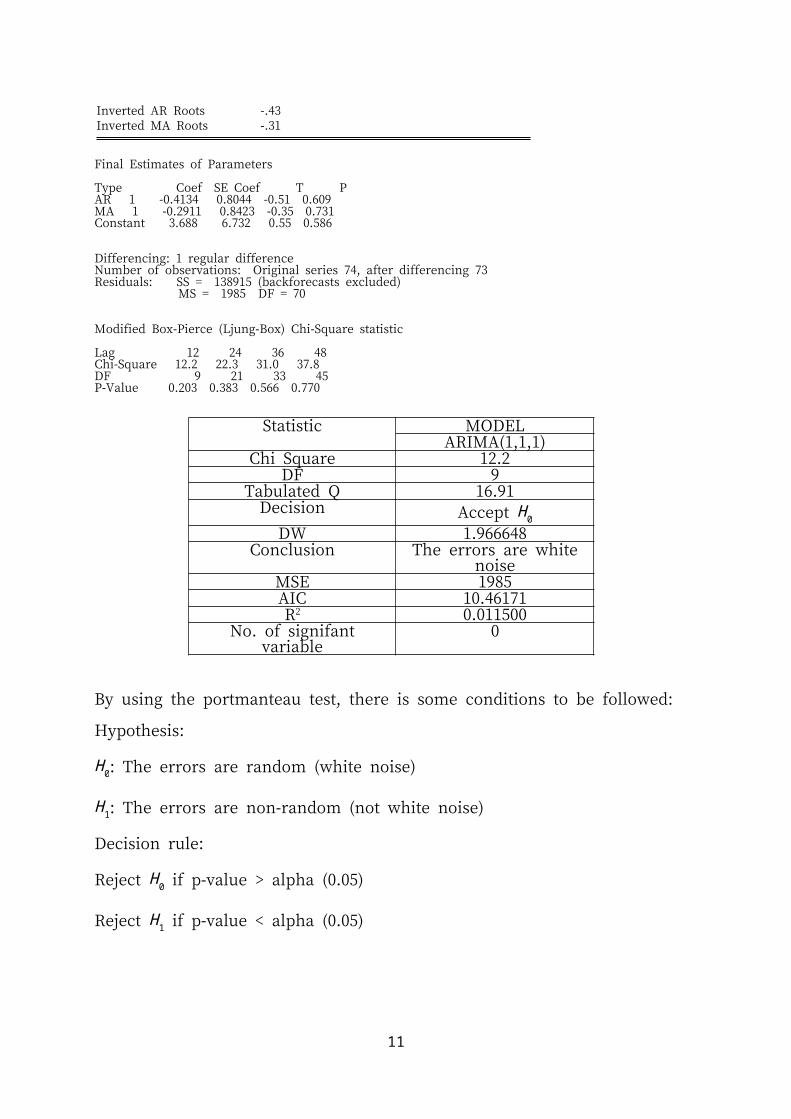
Inverted AR Roots      -.43Inverted MA Roots      -.31

Final Estimates of Parameters

Type Coef SE Coef T PAR 1 -0.4134 0.8044 -0.51 0.609MA 1 -0.2911 0.8423 -0.35 0.731Constant 3.688 6.732 0.55 0.586

Differencing: 1 regular differenceNumber of observations: Original series 74, after differencing 73Residuals: SS = 138915 (backforecasts excluded) MS = 1985 DF = 70

Modified Box-Pierce (Ljung-Box) Chi-Square statistic

Lag 12 24 36 48Chi-Square 12.2 22.3 31.0 37.8DF 9 21 33 45P-Value 0.203 0.383 0.566 0.770

Statistic MODELARIMA(1,1,1)

Chi Square 12.2DF 9

Tabulated Q 16.91Decision Accept H 0

DW 1.966648Conclusion The errors are white noise

MSE 1985AIC 10.46171R2 0.011500

No. of signifant variable 0

By using the portmanteau test, there is some conditions to be followed:

Hypothesis:

H 0: The errors are random (white noise)

H 1: The errors are non-random (not white noise)

Decision rule:

Reject H 0 if p-value > alpha (0.05)

Reject H 1 if p-value < alpha (0.05)

11

Conclusion

Table 1: Summary of MSE Value

MSEModel types

Naïve with trend

Single exponential

Double Exponential

Holt’s method

ARIMA

Estimation

Period

(2/1/14-

8/9/14)

2664.286 1373.823 1363.80 1373.82 1379

Evaluation

Period(9/9/14

-31/12/14)

4268.329 1876.36 1884.48 1876.36 1985

For the estimation part, the smallest MSE is the double exponential which is 1363.80 whereas

the smallest MSE for evaluation part is single exponential which is 1876.36. the overall of the

smallest MSE is from double exponential for the estimation part which is 1363.80. The best

model is from univariate meodelling which is the double exponential since it has the smallest

MSE value.

12