Evidential Probability

and

Objective Bayesian Epistemology

Gregory Wheeler, CENTRIA, New University of LisbonJon Williamson, Philosophy, University of Kent

To appear inPrasanta S. Bandyopadhyay and Malcolm Forster (eds):

Handbook of the Philosophy of Statistics, ElsevierDraft of July 16, 2010

Abstract

In this chapter we draw connections between two seemingly opposingapproaches to probability and statistics: evidential probability on the onehand and objective Bayesian epistemology on the other.

Contents

1 Introduction 2

2 Evidential Probability 2

2.1 Motivation . . . . . . . . . . . . . . . . . . . . . . . . . . . . . . 22.2 Calculating Evidential Probability . . . . . . . . . . . . . . . . . 6

3 Second-order Evidential Probability 9

3.1 Motivation . . . . . . . . . . . . . . . . . . . . . . . . . . . . . . 93.2 Calculating Second-order EP . . . . . . . . . . . . . . . . . . . . 11

4 Objective Bayesian Epistemology 15

4.1 Motivation . . . . . . . . . . . . . . . . . . . . . . . . . . . . . . 154.2 Calculating Objective Bayesian Degrees of Belief . . . . . . . . . 18

5 EP-Calibrated Objective Bayesianism 19

5.1 Motivation . . . . . . . . . . . . . . . . . . . . . . . . . . . . . . 195.2 Calculating EP-Calibrated Objective Bayesian Probabilities . . . 21

6 Conclusion 22

1

1 Introduction

Evidential probability (EP), developed by Henry Kyburg, offers an account ofthe impact of statistical evidence on single-case probability. According to thistheory, observed frequencies of repeatable outcomes determine a probabilityinterval that can be associated with a proposition. After giving a comprehensiveintroduction to EP in §2, in §3 we describe a recent variant of this approach,second-order evidential probability (2oEP). This variant, introduced in Haenniet al. (2008), interprets a probability interval of EP as bounds on the sharpprobability of the corresponding proposition. In turn, this sharp probability canitself be interpreted as the degree to which one ought to believe the propositionin question.

At this stage we introduce objective Bayesian epistemology (OBE), a theoryof how evidence helps determine appropriate degrees of belief (§4). OBE mightbe thought of as a rival to the evidential probability approaches. However, weshow in §5 that they can be viewed as complimentary: one can use the rulesof EP to narrow down the degree to which one should believe a proposition toan interval, and then use the rules of OBE to help determine an appropriatedegree of belief from within this interval. Hence bridges can be built betweenevidential probability and objective Bayesian epistemology.

2 Evidential Probability

2.1 Motivation

Rudolf Carnap (Carnap, 1962) drew a distinction between probability1, whichconcerned rational degrees of belief, and probability2, which concerned statis-tical regularities. Although he claimed that both notions of probability werecrucial to scientific inference, Carnap practically ignored probability2 in thedevelopment of his systems of inductive logic. Evidential probability (EP) (Ky-burg, 1961; Kyburg and Teng, 2001), by contrast, is a theory that gives primacyto probability2, and Kyburg’s philosophical program was an uncompromisingapproach to see how far he could go with relative frequencies. Whereas Bayes-ianism springs from the view that probability1 is all the probability needed forscientific inference, EP arose from the view that probability2 is all that we reallyhave.

The theory of evidential probability is motivated by two basic ideas: proba-bility assessments should be based upon relative frequencies, to the extent thatwe know them, and the assignment of probability to specific individuals shouldbe determined by everything that is known about that individual. Evidentialprobability is conditional probability in the sense that the probability of a sen-tence χ is evaluated given a set of sentences Γδ. But the evidential probabilityof χ given Γδ, written Prob(χ,Γδ), is a meta-linguistic operation similar in kindto the relation of provability within deductive systems.

The semantics governing the operator Prob(·, ·) is markedly dissimilar toaxiomatic theories of probability that take conditional probability as primitive,such as the system developed by Lester Dubbins (Dubbins, 1975; Arlo-Costaand Parikh, 2005), and it also resists reduction to linear (de Finetti, 1974) aswell as lower previsions (Walley, 1991). One difference between EP and the

2

first two theories is that EP is interval-valued rather than point-valued, becausethe relative frequencies that underpin assignment of evidential probability aretypically incomplete and approximate. But more generally, EP assignmentsmay violate coherence. For example, suppose that χ and ϕ are sentences in theobject language of evidential probability. The evidential probability of χ ∧ ϕgiven Γδ might fail to be less than or equal to the evidential probability thatχ given Γδ.1 A point to stress from the start is that evidential probability is alogic of statistical probability statements, and there is nothing in the activityof observing and recording statistical regularities that guarantees that a set ofstatistical probability statements will comport to the axioms of probability. So,EP is neither a species of Carnapian logical probability nor a kind of Bayesianprobabilistic logic.23 EP is instead a logic for approximate reasoning, thus it ismore similar in kind to the theory of rough sets (Pawlak, 1991) and to systemsof fuzzy logic (Dubois and Prade, 1980) than to probabilistic logic.

The operator Prob(·, ·) takes as arguments a sentence χ in the first coordi-nate and a set of statements Γδ in the second. The statements in Γδ representa knowledge base, which includes categorical statements as well as statisticalgeneralities. Theorems of logic and mathematics are examples of categoricalstatements, but so too are contingent generalities. One example of a contingentcategorical statement is the ideal gas law. EP views the propositions “2+2 = 4”and “PV = nRT” within a chemistry knowledge base as indistinguishable an-alytic truths that are built into a particular language adopted for handlingstatistical statements to do with gasses. In light of EP’s expansive view of ana-lyticity, the theory represents all categorical statements as universally quantifiedsentences within a guarded fragment of first-order logic (Andreka et al., 1998).4

Statistical generalities within Γδ, by contrast, are viewed as direct inferencestatements and are represented by syntax that is unique to evidential prob-ability. Direct inference, recall, is the probability assigned a target subclassgiven known frequency information about a reference population, and is oftencontrasted to indirect inference, which is the assignment of probability to a pop-ulation given observed frequencies in a sample. Kyburg’s ingenious idea was tosolve the problem of indirect inference by viewing it as a form of direct infer-ence. Since the philosophical problems concerning direct inference are much lesscontentious than those raised by indirect inference, the unusual properties andbehavior of evidential probability should be weighed against this achievement(Levi, 2007).

Direct inference statements are statements that record the observed fre-quency of items satisfying a specified reference class that also satisfy a particulartarget class, and take the form of

1Specifically, the lower bound of Prob(χ ∧ ϕ,Γδ) may be strictly greater than the lower

bound of Prob(χ,Γδ).2See the essays by Levi and by Seidenfeld in (Harper and Wheeler, 2007) for a discussion

of the sharp differences between EP and Bayesian approaches, particularly on the issue of

conditionalization. A point sometimes overlooked by critics is that there are different systemsof evidential probability corresponding to different conditions we assume to hold. Results

pertaining to a qualitative representation of EP inference, for instance, assume that Γδ is

consistent. A version of conditionalization holds in EP given that there is specific statistical

statement pertaining to the relevant joint distribution. See (Kyburg, 2007) and (Teng, 2007).3EP does inherit some notions from Keynes’s (Keynes, 1921), however, including that

probabilities are interval-valued and not necessarily comparable.4A guarded fragment of first-order logic is a decidable fragment of first-order logic.

3

%�x(τ(�x), ρ(�x), [l, u]).

This schematic statement says that given a sequence of propositional variables�x that satisfies the reference class predicate ρ, the proportion of ρ that alsosatisfies the target class predicate τ is between l and u.

Syntactically, ‘τ(�x), ρ(�x), [l, u]’ is an open formula schema, where ‘τ(·)’ and‘ρ(·)’ are replaced by open first-order formulas, ‘�x’ is replaced by a sequenceof propositional variables, and ‘[l, u]’ is replaced by a specific sub-interval of[0, 1]. The binding operator ‘%’ is similar to the ordinary binding operators(∀, ∃) of first-order logic, except that ‘%’ is a 3-place binding operator overthe propositional variables appearing the target formula τ(�x) and the reference

formula ρ(�x), and binding those formulas to an interval.5 The language Lep

of evidential probability then is a guarded first-order language augmented toinclude direct inference statements. There are additional formation rules fordirect inference statements that are designed to block spurious inference, butwe shall pass over these details of the theory.6 An example of a direct inferencestatement that might appear in Γδ is

%x(B(x), A(x), [.71, .83]),

which expresses that the proportion of A’s that are also B’s lies between 0.71and 0.83.

As for semantics, a model M of Lep is a pair, �D, I�, where D is a two-sorteddomain consisting of mathematical objects, Dm, and a finite set of empiricalobjects, De. EP assumes that there is a first giraffe and a last carbon molecule.I is an interpretation function that is the union of two partial functions, onedefined on Dm and the other on De. Otherwise M behaves like a first-ordermodel: the interpretation function I maps (empirical/mathematical) terms intothe (empirical/mathematical) elements of D, monadic predicates into subsets ofD, n-arity relation symbols into Dn, and so forth. Variable assignments alsobehave as one would expect, with the only difference being the procedure forassigning truth to direct inference statements.

The basic idea behind the semantics for direct inference statements is thatthe statistical quantifier ‘%’ ranges over the finite empirical domain De, notthe field terms l, u that denote real numbers in Dm. This means that the onlyfree variables in a direct inference statement range over a finite domain, whichwill allow us to look at proportions of models in which a sentence is true. Asatisfaction set of an open formula ϕ whose only free n variables are empiricalin the subset of Dn that satisfies ϕ.

A direct inference statement %x(τ(x), ρ(x), [l, u]) is true in M under variableassignment v iff the cardinality of the satisfaction sets for the open formula ρunder v is greater than 0 and the ratio of the cardinality of satisfaction sets forτ(x∗) ∧ ρ(x∗) over the cardinality of the satisfaction sets for ρ(x) (under v) isin the closed interval [l, u], where all variables of x occur in ρ, all variables of τoccur in ρ, and x∗ is the sequence of variables free in ρ but not bound by %x(Kyburg and Teng (2001)).

The operator Prob(·, ·) then provides a semantics for a nonmonotonic conse-quence operator (Wheeler, 2004; Kyburg et al., 2007). The structural properties

5Hereafter we relax notation and simply use an arbitrary variable ‘x’ for ‘�x’.

6See (Kyburg and Teng, 2001).

4

enjoyed by this consequence operator are as follows:7

Properties of EP Entailment: Let |= denote classical consequence andlet ≡ denote classical logical equivalence. Whenever µ ∧ ξ, ν ∧ ξ are sentencesof Lep,

Right Weakening: if µ |≈ ν and ν |= ξ then µ |≈ ξ.

Left Classical Equivalence: if µ |≈ ν and µ ≡ ξ then ξ |≈ ν.

(KTW) Cautious Monotony: if µ |= ν and µ |≈ ξ then µ ∧ ξ |≈ ν.

(KTW) Premise Disjunction: if µ |= ν and ξ |≈ ν then µ ∨ ξ |≈ ν.

(KTW) Conclusion Conjunction: if µ |= ν and µ |≈ ξ then µ |≈ ν ∧ ξ.

As an aside, this qualitative EP-entailment relation presents challenges in han-dling disjunction in the premises since the KTW disjunction property admitsa novel reversal effect similar to, but distinct from, Simpson’s paradox (Ky-burg et al. (2007); Wheeler (2007)). This raises a question over how best toaxiomatize EP. One approach, which is followed by (Hawthorne and Makinson(2007)) and considered in (Kyburg et al. (2007)), is to replace Boolean disjunc-tion by ‘exclusive-or’. While this route ensures nice properties for |≈, it doesso at the expense of introducing a dubious connective into the object languagethat is neither associative nor compositional.8 Another approach explored in(Kyburg et al. (2007)) is a weakened disjunction axiom (KTW Or) that yields asub-System P nonmonotonic logic and preserves the standard properties of thepositive Boolean connectives.

Now that we have a picture of what EP is, we turn to consider the infer-ential behavior of the theory. We propose to do this with a simple ball-drawexperiment before considering the specifics of the theory in more detail in thenext section.

Example 1. Suppose the proportion of white balls (W ) in an urn (U) isknown to be within [.33, 4], and that ball t is drawn from U . These facts arerepresented in Γδ by the sentences, %x(W (x), U(x), [.33, .4]) and U(t).

(i) If these two statements are all that we know about t, i.e., they are theonly statements in Γδ pertaining to t, then Prob(W (t),Γδ) = [.33, .4].

(ii) Suppose additionally that the proportion of plastic balls (P ) that are whiteis observed to be between [.31, .36], t is plastic, and that every plasticball is a white ball. That means that %x(P (x), U(x), [.31, .36]), P (t),and ∀x.P (x) → W (x) are added to Γδ as well. Then there is conflictingstatistical knowledge about t, since either:

1. the probability that ball t is white is between [.33, .4], by reason of%x(W (x), U(x), [.33, .4]), or

7Note that these properties are similar to, but strictly weaker than, the properties of the

class of cumulative consequence relations specified by System P (Kraus et al. (1990)). To

yield the axioms of System P, replace the nonmonotonic consequence operator |∼ for |= in

the premise position of [And*], [Or*], and [Cautious Monotonicity*].8Example: ‘A xor B xor C’ is true if A, B, C are; and ‘(A xor B) xor C’ is not equivalent

to ‘A xor (B xor C)’ when A is false but B and C both true.

5

2. the probability that ball t is white is between [.31, .36], by reason of%x(W (x), P (x), [.31, .36]),

may apply. There are several ways that statistical statements may conflictand there are rules for handling each type, which we will discuss in thenext section. But in this particular case, because it is known that theclass of plastic balls is more specific than the class of balls in U and wehave statistics for the proportion of plastic balls that are also white balls,the statistical statement in (2) dominates the statement in (1). So, theprobability that t is white is in [.31, .36].

(iii) Adapting an example from (Kyburg and Teng, 2001, 216), suppose U ispartitioned into three cells, u1, u2, and u3, and that the following com-pound experiment is performed. First, a cell of U is selected at random.Then a ball is drawn at random from that cell. To simplify matters, sup-pose that there are 25 balls in U and 9 are white such that 3 of 5 ballsfrom u1 are white, but only 3 of 10 balls in u2 and 3 of 10 in u3 are white.The following table summarizes this information.

Table 1: Compound Experiment

u1 u2 u3

W 3 3 3 9W 2 7 7 16

5 10 10 25

We are interested in the probability that t is white, but we have a conflict.Given these over all precise values, we would have Prob(W (t),Γδ) =

925 .

However, since we know that t was selected by performing this compoundexperiment, then we also have the conflicting direct inference statement%x, y(W ∗(x, y), U∗(x, y), [.4, .4]), where U∗ is the set of compound twostage experiments, andW ∗ is the set of outcomes in which the ball selectedis white.9 We should prefer the statistics from the compound experimentbecause they are richer in information. So, the probability that t is whiteis .4.

(iv) Finally, if there happens to be no statistical knowledge in Γδ pertaining tot, then we would be completely ignorant of the probability that t is white.So in the case of total ignorance, Prob(W (t),Γδ) = [0, 1].

We now turn to a more detailed account of how EP calculates probabilities.

2.2 Calculating Evidential Probability

In practice an individual may belong to several reference classes with knownstatistics. Selecting the appropriate statistical distribution among the class of

9Γδ should also include the categorical statements ∀x, y(U∗�x, y� → W (y)), which says that

the second stage of U concerns the proportion of balls that are white, and three statements of

the form�W ∗

(µ, t) ↔ W (t)�, where µ is replaced by u1, u2, u3, respectively. This statement

tells us that everything that’s true of W ∗is true of W , which is what ensures that this conflict

is detected.

6

potential probability statements is the problem of the reference class. The taskof assigning evidential probability to a statement χ relative to a set of evidentialcertainties relies upon a procedure for eliminating excess candidates from theset of potential candidates. This procedure is described in terms of the followingdefinitions.

Potential Probability Statement: A potential probability statement for χwith respect to Γδ is a tuple �t, τ(t), ρ(t), [l, u]�, such that instances of χ ↔ τ(t),ρ(t), and %x(τ(x), ρ(x), [l, u]) are each in Γδ.

Given χ, there are possibly many target statements of form τ(t) in Γδ thathave the same truth value as χ. If it is known that individual t satisfies ρ,and known that between .7 and .8 of ρ’s are also τ ’s, then �t, τ(t), ρ(t), [.7, .8]�represents a potential probability statement for χ based on the knowledge baseΓδ. Our focus will be on the statistical statements %x(τ(x), ρ(x), [l, u]) in Γδ

that are the basis for each potential probability statement.Selecting the appropriate probability interval for χ from the set of potential

probability statements reduces to identifying and resolving conflicts among thestatistical statements that are the basis for each potential probability statement.

Conflict: Two intervals [l, u] and [l�, u�] conflict iff neither [l, u] ⊂ [l�, u�] nor[l, u] ⊃ [l�, u�]. Two statistical statements conflict iff their intervals conflict.Note that conflicting intervals may be disjoint or intersect. For technical reasonsan interval is said to conflict with itself.

Cover: Let X be a set of intervals. An interval [l, u] covers X iff for every[l�, u�] ∈ X, l ≤ l� and u� ≤ u. A cover [l, u] of X is the smallest cover, Cov(X),iff for all covers [l∗, u∗] of X, l∗ ≤ l and u ≤ u∗.

Difference Set: (i) Let X be a non-empty set of intervals and P(X) be thepowerset of X. A non-empty Y ∈ P(X) is a difference set of X iff Y includesevery x ∈ X that conflicts with some y ∈ Y . (ii) Let X be the set of intervalsassociated with a set Γ of statistical statements, and Y be the set of intervalsassociated with a set Λ of statistical statements. Λ is a difference set to Γ iff Yis closed under difference with respect to X.

Example 2. An example might help. Let X be the set of intervals [.30, .40],[.35, .45], [.325, .475], [.50, .55], [.30, .70], [.20, .60], [.10, .90]. There are three setsclosed under difference with respect to X:

(i) {[.30, .40], [.35, .45], [.325, .475], [.50, .55]},

(ii) {[.30, .70], [.20, .60]},

(iii) {[.10, .90]}.

The intuitive idea behind a difference set is to eliminate intervals from a set thatare broad enough to include all other intervals in that set. The interval [.10, .90]is the broadest interval in X. So, it only appears as a singleton difference setand is not included in any other difference set of X. It is not necessary that allintervals in a difference set X be pairwise conflicting intervals. Difference setsidentify the set of all possible conflicts for each potential probability statementin order to find that conflicting set with the shortest cover.

Minimal Cover Under Difference: (i) Let X be a non-empty set ofintervals and Y = {Y1, . . . , Yn} the set of all difference sets of X. The minimal

cover under difference of X is the smallest cover of the elements of Y, i.e., theshortest cover in {Cov(Y1), . . . , Cov(Yn)}.

7

(ii) Let X be the set of intervals associated with a set Γ of statistical state-ments, and Y be the set of all difference sets of X associated with a set Λof statistical statements. Then the minimal cover under difference of Γ is theminimal cover under difference of X.

EP resolves conflicting statistical data concerning χ by applying two prin-ciples to the set of potential probability assignments, Richness and Specificity,to yield a class of relevant statements. The (controversial) principle of Strengthis then applied to this set of relevant statistical statements, yielding a uniqueprobability interval for χ. For discussion of these principles, see (Teng (2007)).

We illustrate these principles in terms of a pair (ϕ,ϑ) of conflicting statisticalstatements for χ, and represent their respective reference formulas by ρϕ andρϑ. The probability interval assigned to χ is the shortest cover of the relevantstatistics remaining after applying these principles.

1. [Richness] If ϕ and ϑ conflict and ϑ is based on a marginal distributionwhile ϕ is based on the full joint distribution, eliminate ϑ.

2. [Specificity] If ϕ and ϑ both survive the principle of richness, and ifρϕ ⊂ ρϑ, then eliminate �τ, ρϑ, [l, u]� from all difference sets.

The principle of specificity says that if it is known that the reference classρϕ is included in the reference class ρϑ, then eliminate the statement ϑ. Thestatistical statements that survive the sequential application of the principle ofrichness followed by the principle of specificity are called relevant statistics.

3. [Strength] Let ΓRS be the set of relevant statistical statements for χwith respect to Γδ, and let the set {Λ1, . . . ,Λn} be the set of differencesets of ΓRS . The principle of strength is the choosing of the minimalcover under difference of ΓRS , i.e., the selection of the shortest cover in{Cov(Λ1), . . . , Cov(Λn)}.

The evidential probability of χ is the minimal cover under difference of ΓRS .We may define Γ�, the set of practical certainties, in terms of a body of

evidence Γδ:

Γ� = {χ : ∃ l, u (Prob(¬χ,Γδ) = [l, u] ∧ u ≤ �)},

or alternatively,

Γ� = {χ : ∃ l, u (Prob(χ,Γδ) = [l, u] ∧ l ≥ 1− �)}.

The set Γ� is the set of statements that the evidence Γδ warrants accepting; wesay a sentence χ is �-accepted if χ ∈ Γ�. Thus we may add to our knowledgebase statements that are nonmonotonic consequences of Γδ with respect to athreshold point of acceptance.

Finally, we may view the evidence Γδ to provide real-valued bounds on ‘de-grees of belief’ owing to the logical structure of sentences accepted into Γδ.However, the probability interval [l, u] associated with χ does not specify arange of equally rational degrees of belief between l and u: the interval [l, u]itself is not a quantity, only l and u are quantities, which are used to specifybounds. On this view, no degree of belief within [l, u] is defensible, which is inmarked contrast to the view offered by Objective Bayesianism.

8

3 Second-order Evidential Probability

3.1 Motivation

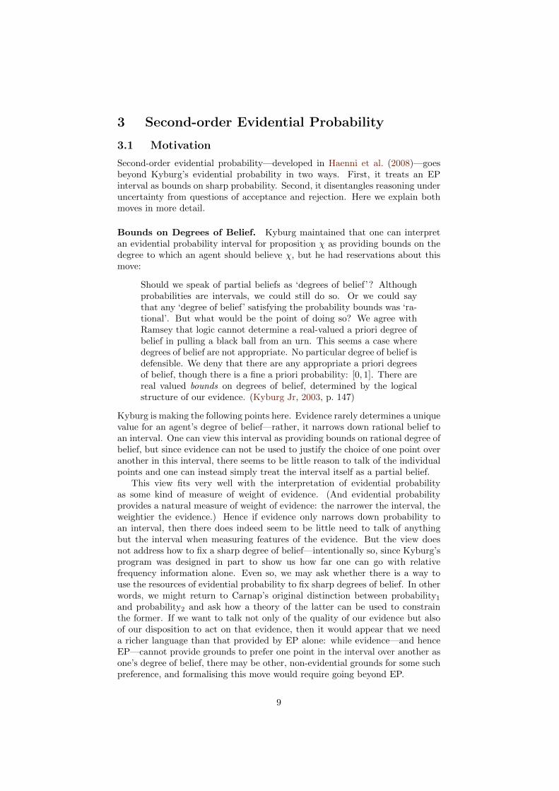
Second-order evidential probability—developed in Haenni et al. (2008)—goesbeyond Kyburg’s evidential probability in two ways. First, it treats an EPinterval as bounds on sharp probability. Second, it disentangles reasoning underuncertainty from questions of acceptance and rejection. Here we explain bothmoves in more detail.

Bounds on Degrees of Belief. Kyburg maintained that one can interpretan evidential probability interval for proposition χ as providing bounds on thedegree to which an agent should believe χ, but he had reservations about thismove:

Should we speak of partial beliefs as ‘degrees of belief’? Althoughprobabilities are intervals, we could still do so. Or we could saythat any ‘degree of belief’ satisfying the probability bounds was ‘ra-tional’. But what would be the point of doing so? We agree withRamsey that logic cannot determine a real-valued a priori degree ofbelief in pulling a black ball from an urn. This seems a case wheredegrees of belief are not appropriate. No particular degree of belief isdefensible. We deny that there are any appropriate a priori degreesof belief, though there is a fine a priori probability: [0, 1]. There arereal valued bounds on degrees of belief, determined by the logicalstructure of our evidence. (Kyburg Jr, 2003, p. 147)

Kyburg is making the following points here. Evidence rarely determines a uniquevalue for an agent’s degree of belief—rather, it narrows down rational belief toan interval. One can view this interval as providing bounds on rational degree ofbelief, but since evidence can not be used to justify the choice of one point overanother in this interval, there seems to be little reason to talk of the individualpoints and one can instead simply treat the interval itself as a partial belief.

This view fits very well with the interpretation of evidential probabilityas some kind of measure of weight of evidence. (And evidential probabilityprovides a natural measure of weight of evidence: the narrower the interval, theweightier the evidence.) Hence if evidence only narrows down probability toan interval, then there does indeed seem to be little need to talk of anythingbut the interval when measuring features of the evidence. But the view doesnot address how to fix a sharp degree of belief—intentionally so, since Kyburg’sprogram was designed in part to show us how far one can go with relativefrequency information alone. Even so, we may ask whether there is a way touse the resources of evidential probability to fix sharp degrees of belief. In otherwords, we might return to Carnap’s original distinction between probability1and probability2 and ask how a theory of the latter can be used to constrainthe former. If we want to talk not only of the quality of our evidence but alsoof our disposition to act on that evidence, then it would appear that we needa richer language than that provided by EP alone: while evidence—and henceEP—cannot provide grounds to prefer one point in the interval over another asone’s degree of belief, there may be other, non-evidential grounds for some suchpreference, and formalising this move would require going beyond EP.

9

Step 1 Evidence {P (ϕ) ∈ [lϕ, uϕ]}Step 2 Acceptance Γδ = {ϕ : lϕ ≥ 1− δ}Step 3 Uncertain reasoning {P (χ) ∈ [lχ, uχ]}Step 4 Acceptance Γε = {χ : lχ≥1− ε}

Figure 1: The structure of (first-order) EP inferences.

Reconciling EP with a Bayesian approach has been considered to be highlyproblematic (Levi, 1977, 1980; Seidenfeld, 2007), and was vigorously resisted byKyburg throughout his life. On the other hand, Kyburg’s own search for an EP-compatible decision theory was rather limited (Kyburg, 1990). It is natural thento explore how to modify evidential probability in order that it might handlepoint-valued degrees of belief and thereby fit with Bayesian decision theory.Accordingly second-order EP departs from Kyburg’s EP by viewing evidentialprobability intervals as bounds on rational degree of belief, P (χ) ∈ Prob(χ,Γδ).In §5 we will go further still by viewing the results of EP as feeding into objectiveBayesian epistemology.

Acceptance and Rejection. If we allow ourselves the language of point-valued degrees of belief, (first-order) EP can be seen to work like this. An agenthas evidence which consists of some propositions ϕ1, . . . ,ϕn and informationabout their risk levels. He then accepts those propositions whose risk levels arebelow the agent’s threshold δ. This leaves him with the evidential certainties,Γδ = {ϕi : P (ϕi)≥1− δ}. From Γδ the agent infers propositions ψ of the formP (χ) ∈ [l, u]. In turn, from these propositions the agent infers the practicalcertainties Γε = {χ : l≥1− ε}. This sequence of steps is depicted in Figure 1.

There are two modes of reasoning that are intermeshed here: on the one handthe agent is using evidence to reason under uncertainty about the conclusionproposition ψ, and on the other he is deciding which propositions to accept andreject. The acceptance mode appears in two places: deciding which evidentialpropositions to accept and deciding whether to accept the proposition χ towhich the conclusion ψ refers.

With second-order EP, on the other hand, acceptance is delayed until all rea-

soning under uncertainty is completed. Then we treat acceptance as a decisionproblem requiring a decision-theoretic solution—e.g., accept those propositionswhose acceptance maximises expected utility.10 Coupling this solution with theuse of point-valued probabilities we have second-order evidential probability(2oEP), whose inferential steps are represented in Figure 2.

There are two considerations that motivate this more strict separation ofuncertain reasoning and acceptance.

First, such a separation allows one to chain inferences—something which isnot possible in 1oEP. By ‘chaining inferences’ we mean that the results of step 2of 2oEP can be treated as an input for a new round of uncertain reasoning, to be

10Note that maximising expected utility is not straightforward in this case since bounds on

probabilities, rather than the probabilities themselves, are input into the decision problem.

EP-calibrated objective Bayesianism (§5) goes a step further by determining point-valued

probabilities from these bounds, thereby making maximisation of expected utility straight-

forward. See Williamson (2008a) for more on the combining objective Bayesianism with a

decision-theoretic account of acceptance.

10

Step 1 Evidence Φ = {P (ϕ) ∈ [lϕ, uϕ]}Step 2 Uncertain reasoning Ψ = {P (χ) ∈ [lχ, uχ]}Step 3 Acceptance {χ : decision-theoretically optimal}

Figure 2: The structure of 2oEP inferences.

recombined with evidence and to yield further inferences. Only once the chainof uncertain reasoning is complete will the acceptance phase kick in. Chainingof inferences is explained in further detail in §3.2.

Second, such a separation allows one to keep track of the uncertainties thatattach to the evidence. To each item of evidence ϕ attaches an interval [lϕ, uϕ]representing the risk or reliability of that evidence. In 1oEP, step 2 ensures thatone works just with those propositions ϕ whose risk levels meet the thresholdof acceptance. But in 2oEP there is no acceptance phase before uncertainreasoning is initiated, so one works with the entirety of the evidence, includingthe risk intervals themselves. While the use of this extra information makesinference rather more complicated, it also makes inference more accurate sincethe extra information can matter—the results of 2oEP can differ from the resultsof 1oEP.

We adopt a decision-theoretic account of acceptance for the following reason.In 1oEP, each act of acceptance uniformly accepts those propositions whoseassociated risk is less than some fixed threshold: δ in step 2 and ε in step 4.(This allows statements to detach from their risk levels and play a role as logicalconstraints in inference.) But in practice thresholds of acceptance depend not somuch on the step in the chain of reasoning as on the proposition concerned, and,indeed, the whole inferential set-up. To take a favourite example of Kyburg’s,consider a lottery. The threshold of acceptance of the proposition the lottery

ticket that the seller is offering me will lose may be higher than that of thecoin with a bias in favour of heads that I am about to toss will land heads andlower than that of the moon is made of blue cheese. This is because nothingmay hang on the coin toss (in which case a 60% bias in favour of heads maybe quite adequate for acceptance), while rather a lot hangs on accepting thatthe moon is made of blue cheese—many other propositions that I have hithertogranted will have to be revisited if I were to accept this proposition. Moreover,if I am going to use the judgement to decide whether to buy a ticket then thethreshold of acceptance of the lottery proposition should plausibly depend onthe extent to which I value the prize. Given these considerations, acceptance ofa proposition can fruitfully be viewed as a decision problem, depending on thedecision set-up including associated utilities (Williamson, 2008a). Again, whilethis is more complicated than the 1oEP solution of modelling acceptance usinga fixed threshold, the subtleties of a full-blown decision-theoretic account canmatter to the resulting inferences.

3.2 Calculating Second-order EP

In this section we will be concerned with developing some machinery to performuncertain reasoning in second-order evidential probability (step 2 in Figure 2).See Haenni et al. (2008) for further details of this approach.

11

Entailment. Let L� be a propositional language whose propositional variablesare of the form ϕ[a,b] for atomic propositions ϕ ∈ L.11 Here L is the languageof (first-order) EP extended to include statements of the form P (χ) ∈ [l, u],and, for proposition ϕ of L, ϕ[a,b] is short for P (ϕ) ∈ [a, b]. Hence in L� wecan express propositions about higher-order probabilities, e.g., P (χ) ∈ [l, u][a,b]

which is short for P (P (χ) ∈ [l, u]) ∈ [a, b]. We write ϕa as an abbreviation ofϕ[a,a].

For µ, ν ∈ L� write µ|≈2oν if ν deductively follows from µ by appealing tothe axioms of probability and the following EP-motivated axioms:

A1: Given ϕ11, . . . ,ϕ

1n, if Prob(χ, {ϕ1, . . . ,ϕn}) = [l, u] is derivable by (first-

order) EP then infer ψ1, where ψ ∈ L is the statement P (χ) ∈ [l, u].

A2: Given ψ1 then infer χ[l,u], where ψ ∈ L is the statement P (χ) ∈ [l, u].

Axiom A1 ensures that EP inferences carry over to 2oEP, while axiom A2 en-sures that probabilities at the first-order level can constrain those at the second-order level.

The entailment relation |≈2o will be taken to constitute core second-order

EP . The idea is that when input evidence Φ consisting of a set of sentences ofL�, one infers a set Ψ of further such sentences using the above consequencerelation. Note that although |≈2o is essentially classical consequence with extraaxioms, it is a nonmonotonic consequence relation since 1oEP is nonmonotonic.But 2oEP yields a strong logic inasmuch as it combines the axioms of probabil-ity with the rules of EP, and so questions of consistency arise. Will there alwaysbe some probability function that satisfies the constraints imposed by 1oEPconsequences of evidence? Not always: see Seidenfeld (2007) for some coun-terexamples. Consequently, some consistency-maintenance procedure needs tobe invoked to cope with such cases. (Of course, some consistency maintenanceprocedure will in any case be required to handle certain inconsistent sets ofevidential propositions, so there may be no extra burden here.) One optionis to consider probability functions satisfying (EP consequences of) maximalsatisfiable subsets of evidential statements, for example. In this paper we willnot commit to a particular consistency-maintenance procedure; we leave thisinteresting question as a topic for further research.

Credal Networks. This entailment relation can be implemented using prob-abilistic networks, as we shall now explain. For efficiency reasons, we make thefollowing further assumptions. First we assume that P is distributed uniformlyover the EP interval unless there is evidence otherwise:

A3: If Φ|≈2oχ[l,u] then P (χ[l�,u�]|Φ) = |[l,u]∩[l�,u�]||[l,u]| , as long as this is consistent

with other consequences of Φ.

Second, we assume that items of evidence are independent unless there is evi-dence of dependence:

A4: If ϕ[a1,b1]1 , . . . ,ϕ[ak,bk]

k ∈ Φ then P (ϕ[a1,b1]1 , . . . ,ϕ[ak,bk]

k ) = P (ϕ[a1,b1]1 ) · · ·P (ϕ[ak,bk]

k ),as long as this is consistent with other consequences of Φ.

11As it stands L�

contains uncountably many propositional variables, but restrictions can

be placed on a, b to circumscribe the language if need be.

12

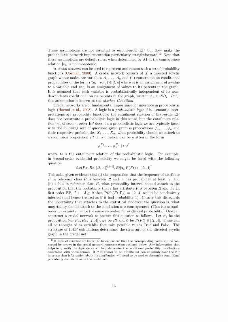
These assumptions are not essential to second-order EP, but they make theprobabilistic network implementation particularly straightforward.12 Note thatthese assumptions are default rules; when determined by A1-4, the consequencerelation |≈2o is nonmonotonic.

A credal network can be used to represent and reason with a set of probabilityfunctions (Cozman, 2000). A credal network consists of (i) a directed acyclicgraph whose nodes are variables A1, . . . , An and (ii) constraints on conditionalprobabilities of the form P (ai | par i) ∈ [l, u] where ai is an assignment of a valueto a variable and par i is an assignment of values to its parents in the graph.It is assumed that each variable is probabilistically independent of its non-descendants conditional on its parents in the graph, written Ai ⊥⊥ ND i | Par i;this assumption is known as the Markov Condition.

Credal networks are of fundamental importance for inference in probabilisticlogic (Haenni et al., 2008). A logic is a probabilistic logic if its semantic inter-pretations are probability functions; the entailment relation of first-order EPdoes not constitute a probabilistic logic in this sense, but the entailment rela-tion |≈2o of second-order EP does. In a probabilistic logic we are typically facedwith the following sort of question: given premiss propositions ϕ1, . . . ,ϕn andtheir respective probabilities X1, . . . , Xn, what probability should we attach toa conclusion proposition ψ? This question can be written in the form

ϕX1

1 , . . . ,ϕXnn |≈ ψ?

where |≈ is the entailment relation of the probabilistic logic. For example,in second-order evidential probability we might be faced with the followingquestion

%x(Fx,Rx, [.2, .4])[.9,1], Rt|≈2oP (Ft) ∈ [.2, .4]?

This asks, given evidence that (i) the proposition that the frequency of attributeF in reference class R is between .2 and .4 has probability at least .9, and(ii) t falls in reference class R, what probability interval should attach to theproposition that the probability that t has attribute F is between .2 and .4? Infirst-order EP, if 1 − δ ≥ .9 then Prob(Ft,Γδ) = [.2, .4] would be conclusivelyinferred (and hence treated as if it had probability 1). Clearly this disregardsthe uncertainty that attaches to the statistical evidence; the question is, whatuncertainty should attach to the conclusion as a consequence? (This is a second-order uncertainty; hence the name second-order evidential probability.) One canconstruct a credal network to answer this question as follows. Let ϕ1 be theproposition %x(Fx,Rx, [.2, .4]), ϕ2 be Rt and ψ be P (Ft) ∈ [.2, .4]. These canall be thought of as variables that take possible values True and False. Thestructure of 1oEP calculations determines the structure of the directed acyclicgraph in the credal net:

12If items of evidence are known to be dependent then the corresponding nodes will be con-

nected by arrows in the credal network representation outlined below. Any information that

helps to quantify the dependence will help determine the conditional probability distributions

associated with these arrows. If P is known to be distributed non-uniformly over the EP

intervals then information about its distribution will need to be used to determine conditional

probability distributions in the credal net.

13

✒✑✓✏ϕ1 ❍❍❍❍❍❥✒✑

✓✏ψ

✒✑✓✏ϕ2

✟✟✟✟✟✯

The conditional probability constraints involving the premiss propositions aresimply their given risk levels:

P (ϕ1) ∈ [.9, 1],

P (ϕ2) = 1.

Turning to the conditional probability constraints involving the conclusion propo-sition, these are determined by 1oEP inferences via axioms A1-3:

P (ψ|ϕ1 ∧ ϕ2) = 1,

P (ψ|¬ϕ1 ∧ ϕ2) = P (ψ|ϕ1 ∧ ¬ϕ2) = P (ψ|¬ϕ1 ∧ ¬ϕ2) = .2.

Finally, the Markov condition holds in virtue of A4, which implies that ϕ1 ⊥⊥

ϕ2. Inference algorithms for credal networks can then be used to infer theuncertainty that should attach to the conclusion, P (ψ) ∈ [.92, 1]. Hence wehave:

%x(Fx,Rx, [.2, .4])[.9,1], Rt|≈2oP (Ft) ∈ [.2, .4][.92,1]

Chaining Inferences. While it is not possible to chain inferences in 1oEP,this is possible in 2oEP, and the credal network representation can just as readilybe applied to this more complex case. Consider the following question:

%x(Fx,Rx, [.2, .4])[.9,1], Rt,%x(Gx, Fx, [.2, .4])[.6,.7]|≈2oP (Gt) ∈ [0, .25]?

As we have just seen, the first two premisses can be used to infer somethingabout Ft, namely P (Ft) ∈ [.2, .4][.92,1]. But now this inference can then be usedin conjunction with the third premiss to infer something about Gt. To work outthe probability bounds that should attach to an inference to P (Gt) ∈ [0, .25],we can apply the credal network procedure. Again, the structure of the graphin the network is given by the structure of EP inferences:

✒✑✓✏ϕ1 ❍❍❍❍❍❥✒✑

✓✏ψ ❍❍❍❍❍❥✒✑

✓✏ϕ2

✟✟✟✟✟✯

✒✑✓✏ψ�

✒✑✓✏ϕ3

✟✟✟✟✟✯

Here ϕ3 is %x(Gx, Fx, [.2, .4]) and ψ� is P (Gt) ∈ [0, .25]; other variables areas before. The conditional probability bounds of the previous example simplycarry over

P (ϕ1) ∈ [.9, 1], P (ϕ2) = 1,

14

P (ψ|ϕ1 ∧ ϕ2) = 1, P (ψ|¬ϕ1 ∧ ϕ2) = .2 = P (ψ|ϕ1 ∧ ¬ϕ2) = P (ψ|¬ϕ1 ∧ ¬ϕ2).

But we need to provide further bounds. As before, the risk level associated withthe third premiss ϕ3 provides one of these:

P (ϕ3) ∈ [.6, .7],

and the constraints involving the new conclusion ψ� are generated by A3:

P (ψ�|ψ ∧ ϕ3) =

|[.2× .6 + .8× .1, .4× .7 + .6× .1] ∩ [0, .25]|

|[.2× .6 + .8× .1, .4× .7 + .6× .1]|= .31,

P (ψ�|¬ψ ∧ ϕ3) = .27, P (ψ�

|ψ ∧ ¬ϕ3) = P (ψ�|¬ψ ∧ ¬ϕ3) = .25.

The Markov Condition holds in virtue of A4 and the structure of EP inferences.Performing inference in the credal network yields P (ψ�) ∈ [.28, .29]. Hence

%x(Fx,Rx, [.2, .4])[.9,1], Rt,%x(Gx, Fx, [.2, .4])[.6,.7]|≈2oP (Gt) ∈ [0, .25][.28,.29].

This example shows how general inference in 2oEP can be: we are not askingwhich probability bounds attach to a 1oEP inference in this example, but ratherwhich probability bounds attach to an inference that cannot be drawn by 1oEP.The example also shows that the probability interval attaching to the conclusioncan be narrower than intervals attaching to the premisses.

4 Objective Bayesian Epistemology

4.1 Motivation

We saw above that evidential probability concerns the impact of evidence upona conclusion. It does not on its own say how strongly one should believe theconclusion. Kyburg was explicit about this, arguing that evidential probabilitiescan at most be thought of as ‘real-valued bounds on degrees of belief, determinedby the logical structure of our evidence’ (Kyburg Jr, 2003, p. 147). To determinerational degrees of belief themselves, one needs to go beyond EP, to a normativetheory of partial belief.

Objective Bayesian epistemology is just such a normative theory (Rosenkrantz,1977; Jaynes, 2003; Williamson, 2005). According to the version of objectiveBayesianism presented in Williamson (2005), one’s beliefs should adhere to threenorms:

Probability: The strengths of one’s beliefs should be representable by proba-bilities. Thus they should be measurable on a scale between 0 and 1, andshould be additive.

Calibration: These degrees of belief should fit one’s evidence. For example,degrees of belief should be calibrated with frequency: if all one knowsabout the truth of a proposition is an appropriate frequency, one shouldbelieve the proposition to the extent of that frequency.

Equivocation: One should not believe a proposition more strongly than theevidence demands. One should equivocate between the basic possibilitiesas far as the evidence permits.

These norms are imprecisely stated: some formalism is needed to flesh themout.

15

Probability. In the case of the Probability norm, the mathematical calculusof probability provides the required formalism. Of course mathematical proba-bilities attach to abstract events while degrees of belief attach to propositions,so the mathematical calculus needs to be tailored to apply to propositions. It isusual to proceed as follows (see, e.g., Paris, 1994). Given a predicate languageL with constants ti that pick out all the members of the domain, and sentencesθ,ϕ of L, a function P is a probability function if it satisfies the following axioms:

P1: If |= θ then P (θ) = 1;

P2: If |= ¬(θ ∧ ϕ) then P (θ ∨ ϕ) = P (θ) + P (ϕ);

P3: P (∃xθ(x)) = limn→∞ P (�n

i=1 θ(ti)).

P1 sets the scale, P2 ensures that probability is additive, and P3, called Gaif-

man’s condition, sets the probability of ‘θ holds of something’ to be the limitof the probability of ‘θ holds of one or more of t1, ..., tn’, as n tends to infinity.The Probability norm then requires that the strengths of one’s beliefs be rep-resentable by a probability function P over (a suitable formalisation of) one’slanguage. Writing P for the set of probability functions over L, the Probabilitynorm requires that one’s beliefs be representable by some P ∈ P.

Calibration. The Calibration norm says that the strengths of one’s beliefsshould be appropriately constrained by one’s evidence E . (By evidence wejust mean everything taken for granted in the current operating context—observations, theory, background knowledge etc.) This norm can be explicatedby supposing that there is some set E ⊆ P of probability functions that sat-isfy constraints imposed by evidence and that one’s degrees of belief should berepresentable by some PE ∈ E. Now typically one has two kinds of evidence:quantitative evidence that tells one something about physical probability (fre-quency, chance etc.), and qualitative evidence that tells one something abouthow one’s beliefs should be structured. In Williamson (2005) it is argued thatthese kinds of evidence should be taken into account in the following way. First,quantitative evidence (e.g., evidence of frequencies) tells us that the physicalprobability function P ∗ must lie in some set P∗ of probability functions. One’sdegrees of belief ought to be similarly constrained by evidence of physical prob-abilities, subject to a few provisos:

C1: E �= ∅.

If evidence is inconsistent this tells us something about our evidence rather thanabout physical probability, so one cannot conclude that P∗ = ∅ and one canhardly insist that PE ∈ ∅. Instead P∗ must be determined by some consistencymaintenance procedure—one might, for example, take P∗ to be determined bymaximal consistent subsets of one’s evidence—and neither P∗ nor E can ever beempty.

C2: If E is consistent and implies proposition θ that does not mention physicalprobability P ∗, then P (θ) = 1 for all P ∈ E.

This condition merely asserts that categorical evidence be respected—it preventsE from being too inclusive. The qualification that θ must not mention physicalprobability is required because in some cases evidence of physical probabilityshould be treated more pliably:

16

C3: If P,Q ∈ P∗ and R = λP +(1−λ)Q for λ ∈ [0, 1] then, other things beingequal, one should be permitted to take R as one’s belief function PE .

Note in particular that C3 implies that, other things being equal, if P ∈ P∗

then P ∈ E; it also implies C1 (under the understanding that P∗ �= ∅). C3 isrequired to handle the following kind of scenario. Suppose for example that youhave evidence just that an experiment with two possible outcomes, a and ¬a,has taken place. As far as you are aware, the physical probability of a is now1 or 0 and no value in between. But this does not imply that your degree ofbelief in a should be 1 or 0 and no value in between—a value of 1

2 , for instance,is quite reasonable in this case. C3 says that, in the absence of other overridingevidence, �P∗� ⊆ E where �P∗� is the convex hull of P∗. The following conditionimposes the converse relation:

C4: E ⊆ �P∗�.

Suppose for example that evidence implies that either P ∗(a) = 0.91 or P ∗(a) =0.92. While C3 permits any element of the interval [0.91, 0.92] as a value forone’s degree of belief PE(a), C4 confines PE(a) to this interval—indeed a valueoutside this interval is unwarranted by this particular evidence. Note that C4implies C2: θ being true implies that its physical probability is 1, so P (θ) = 1for all P ∈ P∗, hence for all P ∈ �P∗�, hence for all P ∈ E.

In the absence of overriding evidence the conditions C1–4 set E = �P∗�. Thissheds light on how quantitative evidence constrains degrees of belief, but onemay also have qualitative evidence which constrains degrees of belief in waysthat are not mediated by physical probability. For example, one may knowabout causal influence relationships involving variables in one’s language: thismay tell one something about physical probability, but it also tells one otherthings—e.g., that if one extends one’s language to include a new variable thatis not a cause of the current variables, then that does not on its own provideany reason to change one’s beliefs about the current variables. These constraintsimposed by evidence of influence relationships, discussed in detail in Williamson(2005), motivate a further principle:

C5: E ⊆ S where S is the set of probability functions satisfying structuralconstraints.

We will not dwell on C5 here since structural constraints are peripheral tothe theme of this paper, namely to connections between objective Bayesianepistemology and evidential probability. It turns out that the set S is alwaysnon-empty, hence C1–5 yield:

Calibration: One’s degrees of belief should be representable by PE ∈ E =�P∗� ∩ S.

Equivocation. The third norm, Equivocation, can be fleshed out by requir-ing that PE be a probability function, from all those that are calibrated withevidence, that is as close as possible to a totally equivocal probability functionP= called the equivocator on L. But we need to specify the equivocator and alsowhat we mean by ‘as close as possible’. To specify the equivocator, first createan ordering a1, a2, . . . of the atomic sentences of L—sentences of the form Ut

17

where U is a predicate or relation and t is a tuple of constants of correspondingarity—such that those atomic sentences involving constants t1, . . . tn−1 occurearlier in the ordering than those involving tn. Then we can define the equivo-cator P= by P=(a

ejj | ae11 ∧ · · · ∧ a

ej−1

j−1 ) = 1/2 for all j and all e1, . . . ej ∈ {0, 1},where a1i is just ai and a0i is ¬ai. Clearly P= equivocates between each atomicsentence of L and its negation. In order to explicate ‘as close as possible’ to P=

we shall appeal to the standard notion of distance between probability functions,the n-divergence of P from Q:

dn(P,Q)df

=1�

e1,...,ern=0

P (ae11 ∧ · · · ∧ aernrn ) log

P (ae11 ∧ · · · ∧ aernrn )

Q(ae11 ∧ · · · ∧ aernrn )

.

Here a1, ..., arn are the atomic sentences involving constants t1, ..., tn; we followthe usual convention of taking 0 log 0 to be 0, and note that the n-divergenceis not a distance function in the usual mathematical sense because it is notsymmetric and does not satisfy the triangle inequality—rather, it is a measureof the amount of information that is encapsulated in P but not in Q. We thensay that P is closer to the equivocator than Q if there is some N such that forn ≥N , dn(P, P=) < dn(Q,P=). Now we can state the Equivocation norm asfollows. For a set Q of probability functions, denote by ↓Q the members of Qthat are closest to the equivocator P=.13 Then,

E1: PE ∈ ↓E.

This principle is discussed at more length in Williamson (2008b). It can beconstrued as a version of the maximum entropy principle championed by EdwinJaynes. Note that while some versions of objective Bayesianism assume that anagent’s degrees of belief are uniquely determined by her evidence and language,we make no such assumption here: ↓E may not be a singleton.

4.2 Calculating Objective Bayesian Degrees of Belief

Just as credal nets can be used for inference in 2oEP, so too can they be usedfor inference in OBE. The basic idea is to use a credal net to represent ↓E,the set of rational belief functions, and then to perform inference to calculatethe range of probability values these functions ascribe to some proposition ofinterest. These methods are explained in detail in Williamson (2008b); here weshall just give the gist.

For simplicity we shall describe the approach in the base case in which theevidence consists of interval bounds on the probabilities of sentences of theagent’s language L, E = {P ∗(ϕi) ∈ [li, ui] : i = 1, . . . , k}, E is consistentand does not admit infinite descending chains; but these assumptions can allbe relaxed. In this case E = �P∗� ∩ S = P∗. Moreover, the evidence can be

written in the language L� introduced earlier: E = {ϕ[l1,u1]1 , . . . ,ϕ[lk,uk]

k }, andthe question facing objective Bayesian epistemology takes the form

ϕ[l1,u1]1 , . . . ,ϕ[lk,uk]

k |≈OBEψ?

13If there are no closest members (i.e., if chains are all infinitely descending: for any member

P of Q there is some P �in Q that is closer to the equivocator than P ) the context may yet

determine an appropriate subset ↓Q ⊆ Q of probability functions that are sufficiently close to

the equivocator; for simplicity of exposition we shall ignore this case in what follows.

18

✒✑✓✏A1 ✒✑

✓✏A2 ✒✑

✓✏A3

Figure 3: Constraint graph.

✒✑✓✏A1

✲✒✑✓✏A2

✲✒✑✓✏A3

Figure 4: Graph satisfying the Markov Condition.

where |≈OBE is the entailment relation defined by objective Bayesian epistemol-ogy as outlined above. As explained in Williamson (2008b), this entailmentrelation is nonmonotonic but it is well-behaved in the sense that it satisfies allthe System-P properties of nonmonotonic logic.

The method is essentially this. First construct an undirected graph, theconstraint graph, by linking with an edge those atomic sentences that appear inthe same item of evidence. One can read off this graph a list of probabilisticindependencies that any function in ↓E must satisfy: if node A separates nodesB and C in this graph then B ⊥⊥ C | A for each probability function in ↓E. Thisconstraint graph can then be transformed into a directed acyclic graph for whichthe Markov Condition captures many or all of these independencies. Finally onecan calculate bounds on the probability of each node conditional on its parentsin the graph by using entropy maximisation methods: each probability functionin ↓E maximises entropy subject to the constraints imposed by E , and one canidentify the probability it gives to one variable conditional on its parents usingnumerical optimisation methods (Williamson, 2008b).

To take a simple example, suppose we have the following question:

∀x(Ux → V x)3/5, ∀x(V x → Wx)3/4, Ut1[0.8,1]

|≈OBEWt?1

A credal net can be constructed to answer this question. There is only oneconstant symbol t1, and so the atomic sentences of interest are Ut1, V t1,Wt1.Let A1 be Ut1, A2 be V t1 and A3 be Wt1. Then the constraint graph G isdepicted in Fig. 3 and the corresponding directed acyclic graph H is depicted inFig. 4. It is not hard to see that P (A1) = 4/5, P (A2|A1) = 3/4, P (A2|¬A1) =1/2, P (A3|A2) = 5/6, P (A3|¬A2) = 1/2; together with H, these probabilitiesyield a credal network. (In fact, since the conditional probabilities are preciselydetermined rather than bounded, we have a special case of a credal net called aBayesian net .) The Markov Condition holds since separation in the constraintgraph implies probabilistic independence. Standard inference methods then giveus P (A3) = 11/15 as an answer to our question.

5 EP-Calibrated Objective Bayesianism

5.1 Motivation

At face value, evidential probability and objective Bayesian epistemology arevery different theories. The former concerns the impact of evidence of physical

19

probability, Carnap’s probability2, and concerns acceptance and rejection; it ap-peals to interval-valued probabilities. The latter theory concerns rational degreeof belief, probability1, and invokes the usual point-valued mathematical notionof probability. Nevertheless the core of these two theories can be reconciled, byappealing to second-order EP as developed above.

2oEP concerns the impact of evidence on rational degree of belief. Givenstatistical evidence, 2oEP will infer statements about rational degrees of belief.These statements can be viewed as constraints that should be satisfied by thedegrees of belief of a rational agent with just that evidence. So 2oEP can bethought of as mapping statistical evidence E to a set E of rational belief func-tions that are compatible with that evidence. (This is a non-trivial mappingbecause frequencies attach to a sequence of outcomes or experimental conditionsthat admit repeated instantiations, while degrees of belief attach to propositions.Hence the epistemological reference-class problem arises: how can one determineappropriate single-case probabilities from information about generic probabili-ties? Evidential probability is a theory that tackles this reference-class problemhead on: it determines a probability interval that attaches to a sentence fromstatistical evidence about repetitions.)

But this mapping from E to E is just what is required by the Calibrationnorm of OBE. We saw in §4 that OBE maps evidence E to E = �P∗� ∩ S, a setof probability functions calibrated with that evidence. But no precise detailswere given as to how �P∗�, nor indeed P∗, is to be determined. In special casesthis is straightforward. For example, if one’s evidence is just that the chanceof a is 1

2 , P ∗(a) = 1/2, then �P∗� = P∗ = {P ∈ P : P (a) = 1/2}. But ingeneral, determining �P∗� is not a trivial enterprise. In particular, statisticalevidence takes the form of information about generic frequencies rather thansingle-case chances, and so the reference-class problem arises. It is here that2oEP can be plugged in: if E consists of propositions of L�—i.e., propositions,including statistical propositions, to which probabilities or closed intervals ofprobabilities attach—then �P∗� is the set of probability functions that satisfythe |≈2o consequences of E .

C6: If E is a consistent set of propositions of L� then �P∗� = {P : P (χ) ∈ [l, u]for all χ, l, u such that E|≈2oχ[l,u]}.

We shall call OBE that appeals to calibration principles C1–6 epistemic-

probability-calibrated objective Bayesian epistemology , or EP-OBE for short. Weshall denote the corresponding entailment relation by |≈EP

OBE.

We see then that there is a sense in which EP and OBE can be viewed ascomplementary rather than in opposition. Of course, this isn’t the end of thematter. Questions still arise as to whether EP-OBE is the right way to flesh outOBE. One can, for instance, debate the particular rules that EP uses to handlereference classes (§2.2). One can also ask whether EP tells us everything we needto know about calibration. As mentioned in §4.1, further rules are needed inorder to handle structural evidence, fleshing out C5. Moreover, both 1oEP and2oEP take statistical statements as input; these statements themselves need tobe inferred from particular facts—indeed EP, OBE and EP-OBE each presumea certain amount of statistical inference. Consequently we take it as understoodthat Calibration requires more than just C1–6.

And questions arise as to whether the alterations to EP that are necessaryto render it compatible with OBE are computationally practical. Second-order

20

EP replaces the original theory of acceptance with a decision theoretic accountwhich will incur a computational burden. Moreover, some thought must be givenas to which consistency maintenance procedure should be employed in practice.Having said this, we conjecture that there will be real inference problems forwhich the benefits will be worth the necessary extra work.

5.2 Calculating EP-Calibrated Objective Bayesian Prob-

abilities

Calculating EP-OBE probabilities can be achieved by combining methods forcalculating 2oEP probabilities with methods for calculating OBE probabilities.Since credal nets can be applied to both formalisms independently, they can alsobe applied to their unification. In fact in order to apply the credal net method toOBE, some means is needed of converting statistical statements, which can beconstrued as constraints involving generic, repeatably-instantiatable variables,to constraints involving the single-case variables which constitute the nodes ofthe objective Bayesian credal net; only then can the constraint graph of §4.2 beconstructed. The 2oEP credal nets of §3.2 allow one to do this, since this kindof net incorporates both statistical variables and single-case variables as nodes.Thus 2oEP credal nets are employed first to generate single-case constraints, atwhich stage the OBE credal net can be constructed to perform inference. Thisfits with the general view of 2oEP as a theory of how evidence constrains rationaldegrees of belief and OBE as a theory of how further considerations—especiallyequivocation—further constrain rational degrees of belief.

Consider the following very simple example:

%x(Fx,Rx, [.2, .5]), Rt, ∀x(Fx → Gx)3/4|≈EP

OBEGt?

Now the first two premisses yield Ft[.2,.5] by EP. This constraint combines withthe third premiss to yield an answer to the above question by appealing to OBE.This answer can be calculated by constructing the following credal net:

✒✑✓✏ϕ ❍❍❍❍❍❥✒✑

✓✏Ft ✲

✒✑✓✏Rt

✟✟✟✟✟✯ ✒✑✓✏Gt

Here ϕ is the first premiss. The left-hand side of this net is the 2oEP net, withassociated probability constraints

P (ϕ) = 1, P (Rt) = 1,

P (Ft|ϕ∧Rt) ∈ [.2, .5], P (Ft|¬ϕ∧Rt) = 0 = P (Ft|ϕ∧¬Rt) = P (Ft|¬ϕ∧¬Rt).

The right-hand side of this net is the OBE net with associated probabilities

P (Gt|Ft) = 7/10, P (Gt|¬Ft) = 1/2.

21

Standard inference algorithms then yield an answer of 7/12 to our question:

%x(Fx,Rx, [.2, .5]), Rt, ∀x(Fx → Gx)3/4|≈EP

OBEGt7/12

6 Conclusion

While evidential probability and objective Bayesian epistemology might at firstsight appear to be chalk and cheese, on closer inspection we have seen that theirrelationship is more like horse and carriage—together they do a lot of work,covering the interface between statistical inference and normative epistemology.

Along the way we have taken in an interesting array of theories—first-orderevidential probability, second-order evidential probability, objective Bayesianepistemology and EP-calibrated OBE—that can be thought of as nonmonotoniclogics.

2oEP and OBE are probabilistic logics in the sense that they appeal tothe usual mathematical notion of probability. More precisely, their entailmentrelations are probabilistic: premisses entail the conclusion if every model ofthe premisses satisfies the conclusion, where models are probability functions.This connection with probability means that credal networks can be appliedas inference machinery. Credal nets yield a perspicuous representation and theprospect of more efficient inference (Haenni et al., 2008).

Acknowledgements

We are grateful to the Leverhulme Trust for supporting this research, and toPrasanta S. Bandyopadhyay, Teddy Seidenfeld and an anonymous referee forhelpful comments.

References

Andreka, H., van Benthem, J., and Nemeti, I. (1998). Modal languages andbounded fragments of predicate logic. Journal of Philosophical Logic, 27:217–274.

Arlo-Costa, H. and Parikh, R. (2005). Conditional probability and defeasibleinference. Journal of Philosophical Logic, 34:97–119.

Carnap, R. (1962). The Logical Foundations of Probability. University ofChicago Press, 2nd edition.

Cozman, F. G. (2000). Credal networks. Artificial Intelligence, 120:199–233.de Finetti, B. (1974). Theory of Probability: A critical introductory treatment.Wiley.

Dubbins, L. E. (1975). Finitely additive conditional probability, conglomerabil-ity, and disintegrations. Annals of Probability, 3:89–99.

Dubois, D. and Prade, H. (1980). Fuzzy Sets and Systems: Theory and Appli-

cations. Kluwer, North Holland.Haenni, R., Romeijn, J.-W., Wheeler, G., and Williamson, J. (2008). Proba-bilistic logic and probabilistic networks. Technical Report 08-01, Universityof Kent Centre for Reasoning. www.kent.ac.uk/reasoning/tr/08-01.pdf.

Harper, W. and Wheeler, G., editors (2007). Probability and Inference: Essays

In Honor of Henry E. Kyburg, Jr. King’s College Publications, London.

22

Hawthorne, J. and Makinson, D. (2007). The quantitative/qualitative watershedfor rules of uncertain inference. Studia Logica, 86(2):247–297.

Jaynes, E. T. (2003). Probability theory: the logic of science. Cambridge Uni-versity Press, Cambridge.

Keynes, J. M. (1921). A Treatise on Probability. Macmillan, London.Kraus, S., Lehman, D., and Magidor, M. (1990). Nonmonotonic reasoning,preferential models and cumulative logics. Artificial Intelligence, 44:167–207.

Kyburg, Jr., H. E. (1961). Probability and the Logic of Rational Belief. WesleyanUniversity Press, Middletown, CT.

Kyburg, Jr., H. E. (1990). Science and Reason. Oxford University Press, NewYork.

Kyburg, Jr., H. E. (2007). Bayesian inference with evidential probability. InHarper, W. and Wheeler, G., editors, Probability and Inference: Essays in

Honor of Henry E. Kyburg, Jr., pages 281–296. King’s College, London.Kyburg, Jr., H. E. and Teng, C. M. (2001). Uncertain Inference. CambridgeUniversity Press, Cambridge.

Kyburg, Jr., H. E., Teng, C. M., and Wheeler, G. (2007). Conditionals andconsequences. Journal of Applied Logic, 5(4):638–650.

Kyburg Jr, H. E. (2003). Are there degrees of belief? Journal of Applied Logic,1:139–149.

Levi, I. (1977). Direct inference. Journal of Philosophy, 74:5–29.Levi, I. (1980). The Enterprise of Knowledge. MIT Press, Cambridge, MA.Levi, I. (2007). Probability logic and logical probability. In Harper, W. andWheeler, G., editors, Probability and Inference: Essays in Honor of Henry E.

Kyburg, Jr., pages 255–266. College Publications.Paris, J. B. (1994). The uncertain reasoner’s companion. Cambridge UniversityPress, Cambridge.

Pawlak, Z. (1991). Rough Sets: Theoretical Aspects of Reasoning about Data.Kluwer, Dordrecht.

Rosenkrantz, R. D. (1977). Inference, method and decision: towards a Bayesian

philosophy of science. Reidel, Dordrecht.Seidenfeld, T. (2007). Forbidden fruit: When Epistemic Probability may nottake a bite of the Bayesian apple. In Harper, W. and Wheeler, G., editors,Probability and Inference: Essays in Honor of Henry E. Kyburg, Jr. King’sCollege Publications, London.

Teng, C. M. (2007). Conflict and consistency. In Harper, W. L. and Wheeler,G., editors, Probability and Inference: Essays in Honor of Henry E. Kyburg,

Jr. King’s College Publications, London.Walley, P. (1991). Statistical Reasoning with Imprecise Probabilities. Chapmanand Hall, London.

Wheeler, G. (2004). A resource bounded default logic. In Delgrande, J. andSchaub, T., editors, NMR 2004, pages 416–422.

Wheeler, G. (2007). Two puzzles concerning measures of uncertainty and thepositive Boolean connectives. In Neves, J., Santos, M., and Machado, J.,editors, Progress in Artificial Intelligence, 13th Portuguese Conference on

Artificial Intelligence, LNAI 4874, pages 170–180, Berlin. Springer-Verlag.Williamson, J. (2005). Bayesian nets and causality: philosophical and compu-

tational foundations. Oxford University Press, Oxford.Williamson, J. (2008a). Aggregating judgements by merging evidence. Journalof Logic and Computation, doi:10.1093/logcom/exn011.

23

Williamson, J. (2008b). Objective Bayesian probabilistic logic. Journal of Al-

gorithms in Cognition, Informatics and Logic, 63:167–183.

24